arXiv:1905.00920v2 [quant-ph] 19 May 2019 Foundations of quantum physics V. Coherent foundations Arnold Neumaier Fakult¨atf¨ ur Mathematik, Universit¨at Wien Oskar-Morgenstern-Platz 1, A-1090 Wien, Austria email: [email protected]http://www.mat.univie.ac.at/~neum May 19, 2019 Abstract. This paper is a programmatic article presenting an outline of a new view of the foundations of quantum mechanics and quantum field theory. In short, the proposed foundations are given by the following statements: • Coherent quantum physics is physics in terms of a coherent space consisting of a line bundle over a classical phase space and an appropriate coherent product. • The kinematical structure of quantum physics and the meaning of the fundamental quan- tum observables are given by the symmetries of this coherent space, their infinitesimal generators, and associated operators on the quantum space of the coherent space. • The connection of quantum physics to experiment is given through the thermal interpre- tation. The dynamics of quantum physics is given (for isolated systems) by the Ehrenfest equations for q-expectations. For the discussion of questions related to this paper, please use the discussion forum https://www.physicsoverflow.org . 1
5.2 Coherent spaces for quantum field theory . . . . . . . . . . . . . . . . . . . . 33
References 36
2
1 Introduction
This paper, the fifth of a series of papers [42, 43, 44, 45] on the foundations of quantum
physics, and the third one of a series of papers (Neumaier [39]) on coherent spaces and their
applications, presents a new view of the foundations for quantum mechanics and quantum
field theory, highlighting the problems and proposing solutions. In short, the proposed
coherent foundations are given by the following statements, made precise later:
Coherent quantum physics is physics in terms of a coherent space consisting of a line
bundle over a classical phase space and an appropriate coherent product. The kinematical
structure of quantum physics and the meaning of the quantum observables1 are given by the
symmetries of this coherent space, their infinitesimal generators, and associated operators
on the quantum space of the coherent space.
The connection of quantum physics to experiment is given through the thermal interpre-
tation. The dynamics of quantum physics is given (for isolated systems) by the Ehrenfest
equations for q-expectations.
The coherent foundations proposed here in a programmatic way resolve the problems with
the traditional presentation of quantum mechanics discussed in Part I [42].
This paper is a programmatic overview article containing the main ideas on coherent spaces
and their relation to quantum physics, not the precise concepts. These are defined and
studied in depth in other papers of the series on coherent spaces, beginning with Neumaier
[40] and Neumaier & Ghaani Farashahi [41]. See also the exposition at the web site
Neumaier [39].
Section 2 gives rigorous definitions of the most basic concepts and results on coherent
spaces, without attempting to be comprehensive, and (together with the next section) a
general outline of a coherent quantum physics, telling the main points of the story with as
few formulas and conceptual details as justifiable.
Section 3 introduces the concept of symmetries (invertible coherent maps) of coherent spaces
and associated quantization procedures. This leads to quantum dynamics, which in special
(completely integrable) situations can be solved in closed form in terms of classical motions
on the underlying coherent space, if the latter has a compatible manifold structure. Spectral
issues can in favorable cases be handled in terms of dynamical Lie algebras. Close relations
to concepts from geometric quantization and Kahler manifolds are pointed out.
In Section 4, we rephrase the formal essentials of the thermal interpretation in a slightly
generalized more abstract setting, to emphasize the essential mathematical features and
1 In the following, these will be called quantities or q-observables to distinguish them fromobservables in the operational sense of numbers obtainable from observation. Similarly, weuse at places q-expectation for the expectation value of quantities.
3
the close analogy between classical and quantum physics. We show how the coherent
variational principle (the Dirac–Frenkel procedure applied to coherent states) can be used to
show that in coarse-grained approximations that only track a number of relevant variables,
quantum mehcnaics exhibits chaotic behavior that, according to the thermal interpretation,
is responsible for the probabilistic features of quantum mechanics.
The final Section 5 defines the meaning of the notion of a field in the abstract setting of
Section 4 and shows how coherent spaces may be used to define relativistic quantum field
theories.
The puzzle of making sense of the foundations of quantum physics held my attention for
many years. Around 2003, I discovered that group coherent states are for many purposes
very useful objects; before, they were for me just a facet that physicists studied who needed
them for quantum optics. In 2007, I realized that apparently all of quantum mechanics and
quantum field theory can be profitably cast into this form, and that coherent states may
provide better theoretical foundations for quantum mechanics and quantum field theory
than the current Fock space approach. Since then I have been putting piece by piece into
the new framework, and always found (after some work) everything nicely fitting. With
each new piece in place, I got insights about how to interpret everything, and things got
simpler and simpler as I proceeded. Or rather, more and more complicated things became
understandable without significant increase of complexity in the new picture. Everything
became much more transparent and intuitive than the traditional mental picture of quantum
physics was.
In the bibliography, the number(s) after each reference give the page number(s) where it is
cited.
Acknowledgments. Earlier versions of this paper benefitted from discussions with Rahel
Knopfel and Mike Mowbray.
2 Coherent spaces
Coherent quantum physics is quantum physics in terms of a coherent space consisting of a
classical phase space and an appropriate coherent product. The kinematical structure and
the meaning of the quantitys are given by the symmetries (invertible coherent maps) of the
coherent space.
This section gives rigorous definitions of the most basic concepts and results, without at-
tempting to be comprehensive, and (together with the next section) a general outline of
a coherent quantum physics, telling the main points of the story with as few formulas
and conceptual details as justifiable. Unexplained details can be found in my papers on
4
coherent spaces (and the references given there). Two of these papers (Neumaier [40]
and Neumaier & Ghaani Farashahi [41]) are already publicly available; others are in
preparation and will become available at my web site [39].
Coherent spaces are a novel mathematical concept, a nonlinear version of Hilbert spaces.
They combine the rich, often highly characteristic variety of symmetries of traditional
geometric structures with the computational tractability of traditional tools from numerical
analysis and statistics.
To get the axioms of a coherent space from those of a Hilbert space, the vector space axioms
are dropped while the notion of inner product and its properties is kept. Every subset of a
real or complex Hilbert space may be viewed as a coherent space. Symmetries induced by
orthogonal resp. unitary transformations become symmetries of the coherent space.
Conversely, every coherent space can be canonically embedded into a complex Hilbert space
(namely its quantum space) in such a way that all its symmetries are realized by unitary
transformations. Thus, in a way, the theory of coherent spaces is just the theory of subsets
of a Hilbert space and their symmetries. However, just as it pays to study the properties of
manifolds independently of their embedding into a Euclidean space, so it appears fruitful
to study the properties of coherent spaces independent of their embedding into a Hilbertspace.
There are close connections to reproducing kernel Hilbert spaces, leading to numerous
applications in quantum physics, complex analysis, statistics, and stochastic processes.
One of the strengths of the coherent space approach is that it makes many different things
look alike, and stays close to actual computations. There are so many applications in
physics and elsewhere that pointing them all out will take a whole book to write. . .
Coherent states and squeezed states in quantum optics, mean field calculations in statistical
mechanics, Hartree–Fock calculations for the electronic states of atoms, semiclassical limits,
integrable systems all belong here. As will be shown in later papers from this series, most
computational techniques in quantum physics can be profitably phrased in terms of coherentspaces.
2.1 Coherent spaces
Fundamental is the notion of a coherent space. It is a nonlinear version of the notion of
a complex Hilbert space: The vector space axioms are dropped while the notion of inner
product, now called a coherent product, is kept. Every coherent space can be embedded
into a Hilbert space extending the coherent product to an inner product.
In informal, traditional terms, a coherent space is roughly a set Z whose elements label
5
certain vectors, called coherent states of a Hilbert space. The quantum space of Z is the
closed subspace formed by the limits of linear combinations of coherent states.
However, one can characterize this situation independent of a Hilbert space setting. Then
a coherent space is a set Z equipped (among others) with a so-called coherent product that
assigns to any two points z, z′ ∈ Z a complex number K(z, z′) satisfying certain coherence
properties. The coherent product is essentially the inner product in the quantum space of
the coherent states with the corresponding classical labels.
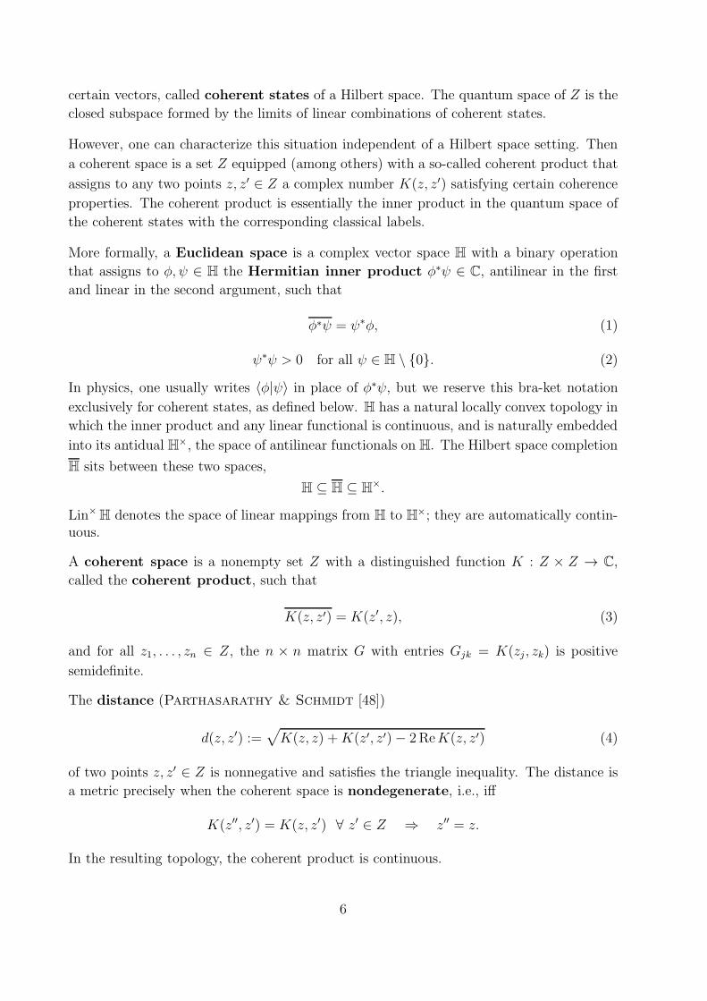
More formally, a Euclidean space is a complex vector space H with a binary operation
that assigns to φ, ψ ∈ H the Hermitian inner product φ∗ψ ∈ C, antilinear in the first
and linear in the second argument, such that
φ∗ψ = ψ∗φ, (1)
ψ∗ψ > 0 for all ψ ∈ H \ {0}. (2)
In physics, one usually writes 〈φ|ψ〉 in place of φ∗ψ, but we reserve this bra-ket notation
exclusively for coherent states, as defined below. H has a natural locally convex topology in
which the inner product and any linear functional is continuous, and is naturally embedded
into its antidual H×, the space of antilinear functionals on H. The Hilbert space completion
H sits between these two spaces,
H ⊆ H ⊆ H×.
Lin×H denotes the space of linear mappings from H to H×; they are automatically contin-uous.
A coherent space is a nonempty set Z with a distinguished function K : Z × Z → C,
called the coherent product, such that
K(z, z′) = K(z′, z), (3)
and for all z1, . . . , zn ∈ Z, the n × n matrix G with entries Gjk = K(zj , zk) is positive
semidefinite.
The distance (Parthasarathy & Schmidt [48])
d(z, z′) :=√K(z, z) +K(z′, z′)− 2ReK(z, z′) (4)
of two points z, z′ ∈ Z is nonnegative and satisfies the triangle inequality. The distance is
a metric precisely when the coherent space is nondegenerate, i.e., iff
K(z′′, z′) = K(z, z′) ∀ z′ ∈ Z ⇒ z′′ = z.
In the resulting topology, the coherent product is continuous.
6
A coherent manifold is a smooth (= C∞) real manifold Z with a smooth coherent product
K : Z × Z → C with which Z is a coherent space. In a nondegenerate coherent manifold,
the infinitesimal distance equips the manifold with a canonical Riemannian metric.
A quantum space Q(Z) of Z is a Euclidean space spanned (algebraically) by a distin-
guished set of vectors |z〉 (z ∈ Z) called coherent states satisfying
〈z|z′〉 = K(z, z′) for z, z′ ∈ Z (5)
with the linear functionals〈z| := |z〉∗
acting on Q(Z). Coherent states with distinct labels are distinct iff Z is nondegenerate.
A construction of Aronszajn [2, 3] (attributed by him to Moore [36]), usually phrased
in terms of reproducing kernel Hilbert spaces, proves the following basic result.
Moore–Aronszajn Theorem. Every coherent space has a quantum space. It is unique
up to isometry.
The antidual Q×(Z) := Q(Z)× of the quantum space Q(Z) is called the augmented
quantum space. It contains the completed quantum space Q(Z), the Hilbert space
completion of Q(Z),
Q(Z) ⊆ Q(Z) ⊆ Q×(Z).
In quantum mechanical applications, Q(Z) is the Hilbert space containing the pure states,
while Q×(Z) also contains unnormalizable wave functions.
Constructing Hilbert spaces from a coherent space and its coherent product is much more
flexible, and hence more powerful, than the standard approach of constructing Hilbert
spaces from a function space and a measure on it. Virtually every Hilbert space arising
in quantum mechanical practice can be neatly constructed as the quantum space of an
appropriate coherent space; the preceding examples gave the first bits of evidence of this.
In a quantum mechanical context, Z is a classical phase space or extended phase space –
typically a symplectic manifold, a Poisson manifold, or a circle or line bundle over such a
manifold that incorporates the classical action variable (encoding the Berry phase under
quantization). For example, the Aharonov–Bohm effect [1] needs the bundle formulation. A
canonical symplectic form is determined by the coherent product. The precise relationship
is the subject of geometric quantization, loosely outlined in Subsection 3.4.
This provides a classical view of the system. On the other hand, the coherent product also
determines its quantum space, whose completion Q(Z) is the Hilbert space of quantum
mechanical state vectors. This provides a quantum view of the system.
Thus coherent spaces allow both a classical and a quantum view of the same system. The
two views are closely related, as the phase space points z ∈ Z label a family of coherent
7
states |z〉, special vectors in the quantum space for which the inner product takes the
simple form
〈z|z′〉 = K(z, z′). (6)
Thus in some sense, the classical phase space and the quantum Hilbert space coexist in the
framework of coherent spaces. The classical phase space is a quotient space of Z under the
equivalence relation that identifies points whose corresponding coherent states differ only
by a scale factor. Thus points in the phase space are in 1-1 correspondence with equivalence
classes of points of Z, hence equivalence classes of labels of coherent states. The quantum
space is the completion of the space spanned by all coherent states. It is a Hilbert space
that can be realized as a space of functions on Z; the coherent states |z〉 are essentially the
functions that map z′ ∈ Z to the coherent product K(z, z′).
If we regard Z as a classical phase space, as often adequate, the functions
ψ(z) := ψT |z〉, ψ ∈ Q(Z).
are those classical phase space functions that have an immediate quantum meaning. Note
that Q×(Z) consists of all complex-valued maps on Z that are continuous in the natural
weak topology induced by the coherent product.
Glauber coherent states (mentioned before) are a particular instantiation of this concept.
A more trivial case to keep in mind is to label all vectors in finite-dimensional Hilbert space
Cn, so that Z = Cn and 〈z|z′〉 = K(z, z′) with
K(z, z′) := z∗z′ =∑
k
zkz′k. (7)
This extends to infinite dimensions (the usual case in most of quantum physics) by replacing
the sum by an appropriate integral, and shows that the traditional way of looking at Hilbert
spaces can be fully accommodated with such a coherent space. However, this choice is poor
from the point of view of the classical-quantum correspondence. As we shall see, there
are far better choices, leading to a much increased flexibility compared to the traditional
approach of defining Hilbert spaces by giving the inner product as a sum or integral. More
importantly, as one works most of the time in Z and very little explicitly in the quantum
space, one can often use classical intuition in quantum situations, and the economy of
classical computations is often preserved.
Finite linear combinations of coherent states form a dense subspace Q(Z) of the Hilbert
space Q(Z). This implies that all quantum mechanical calculations, usually done in an
orthonormal basis, can also be done on the basis of coherent states, and often far more
efficiently. Most conceptual issues can be discussed in coherent terms, too. This makes the
closeness to a classical description very plain, and removes most of the mystery of quantum
physics.
8
The simplest classical systems have a finite number N of states, corresponding to a phase
space Z with N elements. Their dynamics is that of a hopping process, a continuous
time Markov chain determined by consistently specifying transition rates for hopping
from one state to another. More complex classical systems have phase spaces Z that
are finite-dimensional manifolds when there are only finitely many degrees of freedom.
In particular, this is the arena of classical mechanics of point particles, where Z is a
symplectic manifold, or more generally a Poisson manifold. The deterministic dynamics is
defined on Z by Hamilton’s equations, equivalently on phase space functions by means of
the Poisson bracket. Finally, in classical field theory, the phase space Z is an infinite-
dimensional space of fields in 3-dimensional space, the deterministic dynamics on Z is
described by partial differential equations. Often an equivalent dynamics on phase space
functions (now functions on fields) is given in terms of an appropriate Poisson structure on
Z.
The simplest quantum systems have a finite number N of levels, corresponding to a Hilbert
space of dimension N . We may consider them as the quantum version of a Markov chain;
this corresponds to picking an orthonormal basis of N pointer vectors |z〉 and declaring the
coherent product to be K(z, z′) := 〈z|z′〉 = δzz′, thus creating a coherent space Z with N
elements. However, a 2-level quantum system also models a spinning electron at rest in
its ground state. Here the appropriate classical analogue is not the counterintuitive two
state (up-down) model which depends on a distinguished direction and hence sacrifices the
spherical symmetry of the electron, but a 2-sphere in R3, the phase space of a classical
spinning top. To account for the nonintegral spin of the electron, we should in fact take as
classical phase space the double cover of the 2-sphere, given by the unit sphere
Z = {z ∈ C2 | z∗z = 1}
in C2. (The double cover is the so-called Hopf fibration, a nontrivial object.) The 3-sphere
is the same thing as the unit sphere in C2 written in real coordinates. The discussion of
the Hopf fibration in terms of quaternions can be interpreted in terms of Pauli matrices,
giving the traditional approach to 2-level systems. In terms of coherent states, all these
technicalities are hidden – one has the quantum space without having to bother about the
latter. This economy of coherent states becomes more pronounced in more complicated
models, which is the most important one of the reasons why they are studied here.
To get the correct 2-state quantum space, we need to take the trivial coherent product (7)
restricted to Z. Remarkably, the case of a particle of higher spin j has the same phase
space, with the coherent product only slightly changed to
K(z, z′) := (zT z′)2j+1. (8)
Equally remarkably, the coherence conditions are satisfied for this coherent product only if
j = 0, 12, 1, 3
2, . . ., thus naturally accounting for the fact that spin is quantized.
9
In contrast, accounting for arbitrary spin in the traditional fashion based on a (2j+1)-level
system requires a significant amount of machinery already to define the representation.
2.2 Examples
Example: Klauder spaces. The Klauder space KL[V ] over the Euclidean space V is
the coherent manifold Z = C × V of pairs z := [z0, z] ∈ C × V with coherent product
K(z, z′) := ez0+z′0+z
∗z′
. (KL[C] is essentially in Klauder [30]. Its coherent states are
precisely the nonzero multiples of those discovered by Schrodinger [52].) As shown in
detail in Neumaier & Ghaani Farashahi [41], where coherent construction of creation
annihilation operators together with their properties are derived, the quantum spaces of
Klauder spaces are essentially the Fock spaces introduced by Fock [16] in the context of
quantum field theory. They were first presented by Segal [53] in a form equivalent to
the above. The quantum space of KL[Cn] was systematically studied by Bargmann [4].
Example: The Bloch sphere. The unit sphere in C2 is a coherent manifold Z2j+1 with
coherent product K(z, z′) := (z∗z′)2j for some j = 0, 12, 1, 3
2, . . .. It corresponds to the
Poincare sphere (or Bloch sphere) representing a single quantum mode of an atom with
spin j, or for j = 1 the polarization of a single photon mode. The corresponding quantum
space has dimension 2j+1. The associated coherent states are the so-called spin coherentstates.
This example shows that the same set Z may carry many interesting coherent products,
resulting in different coherent spaces with nonisomorphic quantum spaces.
Example: The classical limit. In the limit j → ∞, the unit sphere turns into the
coherent space of a classical spin, with coherent product
K(z, z′) :={1 if z′ = z,0 otherwise.
The resulting quantum space is infinite-dimensional and describes classical stochastic
motion on the Bloch sphere in the Koopman representation.
More generally, any coherent space Z gives rise to an infinite family of coherent spaces
Zn on the same set Z but with modified coherent product Kn(z, z′) := K(z, z′)n with a
nonnegative integer n. (The need for a nonnegative integer is related to Bohr–Sommerfeld
quantization.) The quantum space Q(Zn) is the symmetric tensor product of n copies of
the quantum space Q(Z). If Z has a physical interpretation and the classical limit n→ ∞
exists, it usually has a physical meaning, too.
10
The same abstract quantum system may allow different classical views. The most con-
spicuous expression of this ambiguity is the particle-wave duality, a notion describing
the seemingly paradoxical situation that the same quantum system may be approximately
interpreted either in terms of classical particles or in terms of classical waves, though de-
pending on the circumstances only one of the approximate views may be accurate enough
to be useful. This is accommodated by writing the same Hilbert space in different but
isomorphic ways as the quantum space of different coherent spaces.
Complex quantum systems with finitely many degrees of freedom can be modeled on the
same phase spaces as the corresponding classical systems, and with little additional con-
ceptual effort. (Traditionally, one would need the second quantization formalism or a first
quantized equivalent.) The possibility to describe motion is added by augmenting the
state space by variables for position and momentum. Several particles are accounted for by
taking the direct product of the single-particle phase spaces, the coherent products simply
multiply.
Example: Subsets of a Euclidean space. Any subset Z of a Euclidean space H is a
coherent space with coherent product K(z, z′) := z∗z′. If the linear combinations of Z are
dense in H, then Q(Z) = H. Conversely, any coherent space arises in this way from itsquantum space.
Example: Quantum spaces of entire functions. A de Branges function (de
Branges [10]) is an entire analytic function E : C → C satisfying
|E(z)| < |E(z)| if Im z > 0.
With the coherent product
K(z, z′) :=
E′(z)E(z′)−E ′(z)E(z′) if z′ = z,
E(z)E(z′)− E(z)E(z′)
2i(z − z′)otherwise,
where E ′(z) denotes the derivative of E(z) with respect to z, Z = C is a coherent space.
The corresponding quantum spaces are the de Brange spaces relevant in complex analysis.
Coherent spaces and reproducing kernel Hilbert spaces are mathematically almost equiv-
alent concepts, and there is a vast literature related to the latter. Most relevant for the
present work are the books by Perelomov [50] and Neeb [37]; for applications in proba-
bility and statistics, see also Berlinet & Thomas-Agnan [8].
However, the emphasis in these books is quite different from the present exposition, as they
are primarily interested in properties of the associated functions, while we are primarily
interested in the geometry and symmetry properties and in computational tractability.
11
2.3 New states from old ones
From the set of coherent states it is possible to create a large number of other states
whose inner product is computable by a closed formula. This is important for numerical
applications, since one can pick from the new states created in this fashion a suitable subset
and declare the states belonging to this subset to be the coherent states of a new, derived
coherent space. This way of constructing new coherent spaces from old ones allows one to
apply the general body of techniques for the analysis of coherent spaces and their quantum
properties to the new coherent space. Many known numerical techniques for quantum
physics problems become in this way organized in the same setting.
The first, often useful construction takes a path u(t) in Z and creates new states
[Rtu(t)] := limh↓0
h−1(|u(t+ h)〉 − |u(t)〉
).
We write = ∂jK for the partial derivative with respect to the jth argument of K, and find
the inner products
〈z|[Rtu(t)] = limh↓0
h−1(K(z, u(t+ h))−K(z, u(t))
)= ∂2K(z, u(t))u(t),
[Rtu(t)]∗[Rsv(s)] = lim
h↓0h−1
(〈u(t+ h)|[Rsv(s)]− 〈u(t)|[Rsv(s)]
)
= limh↓0
h−1(∂2K(u(t+ h), v(s))v(t)− ∂2K(u(t), v(s))v(t)
)
= u(t)∂1∂2K(u(t), v(s))v(s).
Similar expressions can be found by taking other smooth parameterizations of submanifolds
of Z, and taking limits corresponding to first order or higher order partial derivatives.
A trivial construction is to take linear combinations
[α, y] :=∑
k
αk|yk〉,
where α is a finite sequence of complex numbers αk and y is a finite sequence of points
yk ∈ Z. The inner products are given by
〈z|[α, y] =∑
k
αkK(z, yk),
[α, y]∗[α′, y]′ =∑
j,k
αjα′kK(yj, yk),
This also works for infinite sequences provided the right hand sides are always absolutely
convergent, and with sums replaced by integrals for weighted integrals∫α(x)|y(x)〉dµ(x),
12
provided the corresponding integrals on the right hand sides are always absolutely conver-
gent. Of course, all these recipes can also be combined.
We see that, unlike in traditional Hilbert spaces, where the calculation of inner products
always requires to evaluate often high-dimensional integrals, here the calculation of inner
products is much simpler, often only taking sums and derivatives.
3 Coherent spaces and quantization
This section introduces the concept of symmetries (invertible coherent maps) of coherent
spaces and associated quantization procedures. This leads to quantum dynamics, which in
special (completely integrable) situations can be solved in closed form in terms of classical
motions on the underlying coherent space, if the latter has a compatible manifold structure.
Spectral issues can in favorable cases be handled in terms of dynamical Lie algebras. Close
relations to concepts from geometric quantization and Kahler manifolds are pointed out.
3.1 Symmetries
Symmetries of a coherent space are transformations of the space that preserve the coherent
structure. They generalize canonical transformations of a symplectic manifold, which is the
special case of classical mechanics of point particles. More specifically, a symmetry of a
coherent space Z is a bijection A of Z with the property that
K(z, Az′) = K(AT z, z′) (9)
for another bijection AT .
Let Z be a coherent space. A map A : Z → Z is called coherent if there is an adjoint
map A∗ : Z → Z such that
K(z, Az′) = K(A∗z, z′) for z, z′ ∈ Z (10)
If Z is nondegenerate, the adjoint is unique, but not in general.
A symmetry of Z is an invertible coherent map on Z with an invertible adjoint.
Coherent maps form a semigroup CohZ with identity; the symmetries form a group.
An isometry is a coherent map A that has an adjoint satisfying A∗A = 1. An invertible
isometry is called unitary.
Symmetries of a coherent space often represent the dynamical symmetries (see, e.g., barut
& Raczka [7]) of an associated exactly solvable classical system. For example, if Z is a
13
line bundle over a symplectic phase space, the symmetries would be all linear symplectic
maps and their central extensions. (But only some of them preserve the Hamiltonian and
hence are symmetries of the system with this Hamiltonian.)
In the coherent space formed by a subset Z of Cn closed under conjugation, with coherent
product K(z, z′) := zT z′, all n × n matrices mapping Z into itself are (in this particular
case linear) coherent maps, and all invertible matrices are symmetries.
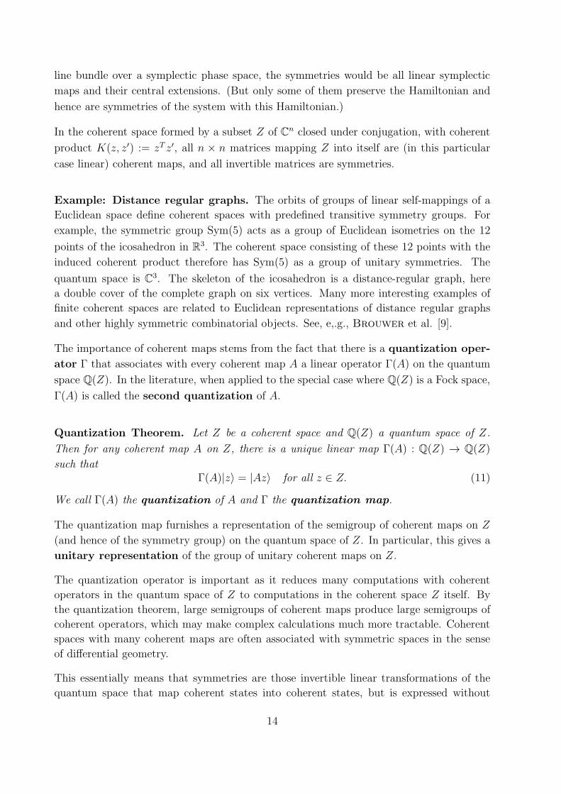
Example: Distance regular graphs. The orbits of groups of linear self-mappings of a
Euclidean space define coherent spaces with predefined transitive symmetry groups. For
example, the symmetric group Sym(5) acts as a group of Euclidean isometries on the 12
points of the icosahedron in R3. The coherent space consisting of these 12 points with the
induced coherent product therefore has Sym(5) as a group of unitary symmetries. The
quantum space is C3. The skeleton of the icosahedron is a distance-regular graph, here
a double cover of the complete graph on six vertices. Many more interesting examples of
finite coherent spaces are related to Euclidean representations of distance regular graphs
and other highly symmetric combinatorial objects. See, e,.g., Brouwer et al. [9].
The importance of coherent maps stems from the fact that there is a quantization oper-
ator Γ that associates with every coherent map A a linear operator Γ(A) on the quantum
space Q(Z). In the literature, when applied to the special case where Q(Z) is a Fock space,
Γ(A) is called the second quantization of A.
Quantization Theorem. Let Z be a coherent space and Q(Z) a quantum space of Z.
Then for any coherent map A on Z, there is a unique linear map Γ(A) : Q(Z) → Q(Z)
such that
Γ(A)|z〉 = |Az〉 for all z ∈ Z. (11)
We call Γ(A) the quantization of A and Γ the quantization map.
The quantization map furnishes a representation of the semigroup of coherent maps on Z
(and hence of the symmetry group) on the quantum space of Z. In particular, this gives a
unitary representation of the group of unitary coherent maps on Z.
The quantization operator is important as it reduces many computations with coherent
operators in the quantum space of Z to computations in the coherent space Z itself. By
the quantization theorem, large semigroups of coherent maps produce large semigroups of
coherent operators, which may make complex calculations much more tractable. Coherent
spaces with many coherent maps are often associated with symmetric spaces in the sense
of differential geometry.
This essentially means that symmetries are those invertible linear transformations of the
quantum space that map coherent states into coherent states, but is expressed without
14
reference to the quantum space. This has very important implications for practical com-
putations, reducing computations in the quantum space to simple computations in the
coherent space. In particular, this makes certain problems easily exactly solvable that are
in the traditional position or momentum representations nearly intractable. For example,
the calculation of q-expectations requires in the traditional setting the evaluation of an
integral over configuration space. In case of field theory, the configuration space is infinite-
dimensional, and already a rigorous definition of such integrals is very difficult. Moreover,
finding closed formulas for integrals in high or infinite dimensions is more an art than a
science. In contrast, in the coherent space approach, many q-expectations of interest can
be obtained by differentiation, which is a fully algorithmic process.
In case of the trivial coherent product (7), equation (9) holds for every n× n matrix with
the usual matrix transpose. This motivates the general case, and shows in particular that
the trivial coherent space has the general linear group GL(n,C) of invertible complex
n × n matrices as its group of symmetries. For virtually all quantum systems of interest
there is a large classical dynamical symmetry group, which describes the symmetries
of the underlying coherent space. Typically, this symmetry group is a (possibly infinite-
dimensional) Lie group, much larger than the symmetry group of the system itself – which
is the subgroup commuting with the Hamiltonian (in the nonrelativistic case) or preserving
the action (in the relativistic case).
Example: Mobius space. The Mobius space Z = {z ∈ C2 | |z1| > |z2|} is a coherent
manifold with coherent product K(z, z′) := (z1z′1− z2z
′2)
−1. A quantum space is the Hardy
space of analytic functions on the complex upper half plane with Lebesgue integrable limit
on the real line. The Mobius space has a large semigroup of coherent maps (a semigroup
of compressions, Olshanski [46]) consisting of the matrices A ∈ C2×2 such that
α := |A11|2 − |A21|
2, β := A11A12 − A21A22, γ := |A22|2 − |A12|
2
satisfy the inequalities
α > 0, |β| ≤ α, γ ≤ α− 2|β|.
It contains as a group of symmetries the group GU(1, 1) of matrices preserving the Hermi-
tian form |z1|2 − |z2|
2 up to a positive factor.
Highest weight representations. The example of the Mobius space generalizes to a
large class of exactly solvable classical systems with finitely many degrees of freedom, cor-
responding to the coherent states from group representations discussed in Zhang et al.
[59] and Simon [54], which are close to being computable (though not all needed details
are in these papers). The constructions relate to central extensions of all semisimple Lie
groups and associated symmetric spaces or symmetric cones and their line bundles.
These provide many interesting examples of coherent manifolds. This follows from work on
15
coherent states constructed from highest weight representations, discussed in monographs
by Perelomov [50], by Faraut & Koranyi [15], by Neeb [37].
Coherent states from highest weight representations induce on the corresponding coadjoint
orbit a measure, a metric, a symplectic form, and an associated symplectic Poisson bracket.
(See the Zhang et al. [59] survey for details from a physical point of view. The Poisson
bracket defines a Lie algebra on phase space functions (C∞ functions on the coadjoint
orbit, hence an associated group of Hamiltonian diffeomorphisms, and the coherent state
approach effectively quantizes this group. All this can be reconstructed directly from the
associated coherent spaces. In particular, the nonclassical states of light in quantum optics
called squeezed states are described by coherent spaces corresponding to themetaplectic
group; cf. related work by Neretin [38].
3.2 q-observables and dynamics
We now assume that Z is a coherent manifold. This means that Z carries a C∞-manifoldstructure with respect to which the coherent product is smooth (C∞). The relevant observ-
ables of the classical system are the discrete symmetries and the infinitesimal generators of
the 1-parameter groups of symmetries that are smooth on the coherent product. They are
promoted to q-observables of the corresponding quantum system through the quantization
map. For a symmetry A, the corresponding q-observable is Γ(A). For an infinitesimal
symmetry X , i.e., an element of the Lie algebra of generators of 1-parameter groups of the
symmetry group), the corresponding quantum symmetry, acting on the quantum space
of Z, is the q-observable given by the strong limit
dΓ(X) := lims↓0
Γ(eisX)− 1
is.
Note that
dΓ(X + Y ) = dΓ(X) + dΓ(Y ), edΓ(X) = Γ(eX).
The quantization theorem from Subsection 3.1 may be regarded as a generalized Noether
principle that automatically promotes all symmetries of Z to dynamical symmetries of the
corresponding quantum system.
Thus a coherent space contains intrinsically all information needed to interpret the quantum
system, including that about which operators may be treated as q-observables.
The dynamics of a physical system is traditionally given by a Hamiltonian, a symmetric
and Hermitian expression H in the q-observables. If the coherent space is in fact a coherent
manifold, the classical dynamics determined by the Hamiltonian is given by a Poisson
bracket canonically associated to the coherent space through variation of the so-called
Dirac–Frenkel action discussed in Subsection 4.4 below. (Classical mechanics on Poisson
16
manifolds, the most general setting for the dynamics in closed classical systems, is discussed
in detail in Marsden & Ratiu [34]. Less general is classical mechanics on symplectic
manifolds, and even more restricted is classical mechanics on cotangent bundles, which
includes classical mechanics on phase space R6N for systems of N particles in Cartesian
coordinates.)
In a classical Hamiltonian system, the dynamics of a phase space function f is given by
f = H ∠ f where f ∠ g = {g, f} in terms of the Poisson bracket. For an N -particle system
with particle positions qj and particle momenta pj , specializing this to f = qj and g = pjgives the classical equations of motion. In a quantum system, one has the same in the
Heisenberg picture, and according to every textbook, the resulting dynamics is equivalent
to the Schrodinger equation in the Schrodinger picture.
Exactly solvable systems. In the special case where the classical Hamiltonian is an
infinitesimal symmetry of Z, and hence the quantum Hamiltonian has the form Γ(H), the
quantization lifts the classical phase space trajectory to a quantum trajectory. Thus if the
Lie algebra of q-observables contains the Hamiltonian (and in some slightly more general
situations), the quantum dynamics has the special feature that coherence is dynamically
preserved. In terms of the Hamiltonian, the dynamics for pure quantum states ψ is tradi-
tionally given by the time-dependent Schrodinger equation
ihdψ
dt= dΓ(H)ψ
for the corresponding quantum Hamiltonian dΓ(H). A dynamical symmetry preserved
by H (in the classical case) or dΓ(H) (in the quantum case) is a true symmetry of the
corresponding classical or quantum system. The Fourier transform ψ(E) satisfies the time-
independent Schrodinger equation
dΓ(H)ψ = Eψ. (12)
The following result shows that the solution of Schrodinger equations with a sufficiently
nice Hamiltonian can be reduced to solving differential equations on Z.
3.1 Theorem. Let Z be a coherent space, and G be a Lie group of coherent maps with
associated Lie algebra L. Let H(t) ∈ L be a Hamiltonian with possibly time-dependent
coefficients. Then the solution of the initial value problem
ih∂
∂tψt = dΓ(H(t))ψt, ψ0 = |z0〉 (13)
with z0 ∈ Z has for all times t ≥ 0 the form of a coherent state, ψt = |z(t)〉 with the
trajectory z(t) ∈ Z defined by the initial value problem
ihz(t) = H(t)z(t), z(0) = z0.
17
This means that if a system is at some time in a coherent state it will be at all times in a
coherent state.
This conservation of coherence has the consequence that the quantum system is exactly
solvable. This means that the complete solution of the dynamics of the quantum system
can be reduced to the solution of the corresponding classical system. Effectively, the partial
differential equations of quantum mechanics in the quantum space are solved in terms of
ordinary differential equations on the underlying coherent space. In many cases, this implies
that the spectrum can be determined explicitly in terms of the representation theory of the
corresponding Lie algebras.
More generally (see, e.g., Iachello [24]), we have an exactly solvable system whenever
the Hamiltonian H(t) is a linear combination of infinitesimal symmetries with coefficents
given by Casimirs of the Lie algebra L of infinitesimal symmetries, i.e., in the classical
case central elements of the Lie–Poisson algebra C∞(L∗), and in the quantum case of the
universal enveloping algebras of L. On any orbit of the symmetry group, these Casimirs
are represented by multiplication with a constant. One can therefore extend the coherent
space Z without changing the quantum space by treating the corresponding multiples of
the coherent states as new coherent states of an extended coherent space whose elements
are labelled by pairs of elements of Z and appropriate multipliers. This turns the algebra
of Casimirs into an abelian group of symmetries of the extended coherent space, which,
together with original symmetries provides an action of a central extension of the original
symmetry group as a symmetry group of the extended coherent space.
The time-independent Schrodinger equation (12) generalizes easily to a more general im-
plicit Schrodinger equation I(E)ψ = 0. This more general formulation fits naturally
the coherent space setting, and everything said so far (corresponding to I(E) = E−dΓ(H))
generalizes to the general implicit formulation.
3.3 Dynamical Lie algebras
A quantum dynamical problem can often be reduced to finding the spectrum of a physical
system defined by an implicit Schrodinger equation
I(E)ψ = 0 (14)
with an energy-dependent system operator I(E), and ψ in the antidual of some Euclidean
space H. A nonlinear I(E) typically appears in reduced effective descriptions of systems
derived from a more complicated Hamiltonian setting and in relativistic systems. (The
antidual is needed to account for a possible continuous spectrum.)
This section discusses implicit Schrodinger equations for the exactly solvable case where
the system operator I(E) is contained in a Lie algebra L with known representation theory.
18
This is the setting where a tractable dynamical symmetry group for the Hamiltonian is
known and covers many interesting systems.
For example, the system operator I(E) = p20 − p2 − (mc)2 with p0 = E/c describes a free
spin 0 particle. This generalizes to a quadratic implicit Schrodinger equation
(π2 −
igeh
cSS · F(x)− (mc)2
)ψ = 0 (15)
for a particle of charge e, mass m, and arbitrary spin in an electromagnetic field. Here
π =
(π0π
):= p + ehA(x) (16)
is a gauge invariant 4-vector, SS is the 3-dimensional spin vector representing the intrinsic
angular momentum of a particle of spin j = 0, 12, 1, . . ., the 3-vector F(x) = E(x) + icB(x)
is the Riemann–Silberstein vector encoding the electric field E(x) and the magnetic field
B(x), and g is the dimensionless g-factor of the magnetic moment
µs := −gµB
hSS,
where µB is a constant called the Bohr magneton, and ψ is a wave function with s = 2j+1
components. For spin j = 1/2, we have s = 2 components, hence, being second order, 4
local degrees of freedom, corresponding to the 4 components of the (first order) Dirac
equation, which is equivalent to the special case g = 2.
In the special case where the dependence on E is linear, we have
I(E) = EM −N (17)
with fixed M,N ∈ L. This covers the simple case of a harmonic oscillator, where M = 1,
N = 12(p2/m+Kq2) is the Hamiltonian, and the Lie algebra is the oscillator algebra, with
generators 1, p, q, H (or, in complex form, 1, a, a∗, a∗a). It also covers a family of practically
relevant exactly solvable systems with Lie algebra L = so(2, 1)⊕C = su(1, 1)⊕C discussed
in detail in the book by Wybourne [57], containing among others the case of a particle of
mass m in a Coulomb field, with M = r = |q| and N =MH , where
H =1
2mv2 −
α
|q|
is the Coulomb Hamiltonian.
If I(E) belongs for all E to some Lie algebra L acting on H in a (reducible or irreducible)
representation then L is called a dynamical Lie algebra2of the problem.
2 One can always take the dynamical Lie algebra to be the Lie algebra LinH of all linear operatorson the nuclear space H. For this choice, the dynamical Lie algebra offers no advantage over the standardtreatment. Therefore it is usually understood that the dynamical Lie algebra is much smaller than LinH,although mathematically there is no such restriction.
19
In general, the requirement for a dynamical symmetry group is just that all quantities of
physical interest in the system can be expressed in the Lie–Poisson algebra (in the classical
case) or the universal enveloping algebra (in the quantum case) of the corresponding Lie
algebra. In this case, the label “dynamical” is a misnomer, and kinematic symmetry
group would be more appropriate. The kinematic symmetry group is an integral part of the
Hamiltonian or Lagrangian setting; so one usually gets it directly from the formulation and
a look at the obvious symmetries. For any anharmonic oscillator it is Sp(2); for any system
of N particles in R3 it is the symplectic group Sp(6N), generated by the inhomogeneous
quadratics in p and q.
If a problem has a dynamical symmetry group such that the (discrete or continuous) spec-
trum of all elements of its Lie algebra L is exactly computable then the spectrum of the
system can be found exactly. In the best understood cases, L is a finite-dimensional semisim-
ple Lie algebra. Here everything is tractable more or less explicitly since the representation
theory of these Lie algebras and their corresponding groups is fully understood. A problem
solvable in this way is called integrable.
The spectrum of the nonlinear eigenvalue problem (14) is the set Spec I of all E ∈ C such
that I(E) is not invertible. In terms of (generalized) eigenvalues and eigenvectors of I(E),
I(E)|ξ, E〉 = λ(ξ, E)|ξ, E〉,
where ξ is a label distinguishing different eigenvectors |ξ, E〉 in a (generalized) orthonormal
basis of the eigenspace corresponding to the eigenvalue E. To cover the continuous spectrum
(where eigenvectors are unnormalized, hence do not belong to the Hilbert space), we work
in a Euclidean space H on which the Hamiltonian acts as a linear operator. The Hilbert
space of the problem is then the completion H of this space, and H ⊆ H ⊆ H× is a Gelfand
triple. Therefore
I(E)|ξ, E〉 = 0 whenever λ(ξ, E) = 0.
ThusSpec I = {E ∈ R | λ(ξ, E) = 0 for some ξ ∈ Spec I(E)}
Moreover, it is easy to see that all eigenvectors of the nonlinear eigenvalue problem have
the form |ξ, E〉. Thus the spectrum is given by the set of solutions of the nonlinear equation
λ(ξ, E) = 0.
In many cases of interest (e.g., cf. Subsection 4.1, when L is a Lie ∗-algebra), L = L0 ⊕C;
then we may write
I(E) := m(E)X(E)− k(E), (18)
where m(E) and k(E) are scalars not vanishing simultaneously, and X(E) ∈ L0. If
X(E)|ξ, E〉 = ξ|ξ, E〉
20
is a complete system of (generalized) eigenvalues and eigenvectors of X(E) then
Schlichenmaier [51]) proceeds from a symplectic manifold K. It constructs (in the group
case in terms of integral3 cohomology) a polarization that defines a Hermitian line bundle
Z = CK and an associated Kahler potential (which is essentially the logarithm of the
coherent product). This potential turns K into a Kahler manifold with a natural Kahler
metric, Kahler measure, and symplectic Kahler bracket. If the Kahler metric is definite
(which is always the case if Z is a compact symmetric space), there is an associated Hilbert
space of square integrable functions on which quantized operators can be defined by a recipe
of van Hove [23].
An involutive coherent manifold is a coherent manifold Z equipped with a smooth map-
ping that assigns to every z ∈ Z a conjugate z ∈ Z such that z = z andK(z, z′) = K(z, z′)
for z, z′ ∈ Z. Under additional conditions, an involutive coherent manifold carries a canoni-
cal Kahler structure turning it into a Kahler manifold. For semisimple finite-dimensional
Lie algebras, the irreducible highest weight representations have nice coherent space for-
mulations. In the literature, the logarithm of the coherent product figures under the name
of Kahler potential. Zhang et al. [59] relate the latter to coherent states. The coherent
quantization of Kahler manifolds is equivalent to traditional geometric quantization of
Kahler manifolds. But in the coherent setting, quantization is not restricted to finite-
dimensional manifolds, which is important for quantum field theory.
The coherent product and the conjugation are C∞-maps on the line bundle. In order that
this line bundle exists, the symplectic manifold must also carry a positive definite Kahler
potential F : Z × Z → C satisfying a generalized Bohr–Sommerfeld quantization
condition defined by the integrality of some cohomological expression. In this case, Z is a
projective coherent space with coherent product
K(z, z′) := e−F (z,z′).
The quantum space of the projective coherent space carries the representation satisfying the
conditions of a successful geometric quantization. This procedure, called Berezin quanti-
zation, is the most useful way of performing geometric quantization; see, e.g., Schlichen-
maier [51].
3 Integral cohomology apparently corresponds to the fact that the line bundle can in fact be viewed asa U(1)-bundle so that phases are well-defined.
23
4 The thermal interpretation in terms of Lie algebras
Coherent quantum physics on a coherent space Z is related to physical reality by means of
the thermal interpretation, discussed in detail in Part II [43] and applied to measurement
in Part III [44] of this series of papers. We rephrase the formal essentials of the thermal
interpretation in a slightly generalized more abstract setting, to emphasize the essential
mathematical features and the close analogy between classical and quantum physics. We
show how the coherent variational principle (the Dirac–Frenkel procedure applied to coher-
ent states) can be used to show that in coarse-grained approximations that only track a
number of relevant variables, quantum mehcnaics exhibits chaotic behavior that, accord-
ing to the thermal interpretation, is responsible for the probabilistic features of quantum
mechanics.
4.1 Lie ∗-algebras
A (complex) Lie algebra is a complex vector space L with a distinguished Lie product,
a bilinear operation on L satisfying X ∠X = 0 for X ∈ L and the Jacobi identity
X ∠ (Y ∠Z) + Y ∠ (Z ∠X) + Z ∠ (X ∠ Y ) = 0 for X, Y, Z ∈ L.
A Lie ∗-algebra is a complex Lie algebra L with a distinguished element 1 6= 0 called one
and a mapping ∗ that assigns to every X ∈ L an adjoint X∗ ∈ L such that
(X + Y )∗ = X∗ + Y ∗, (X ∠ Y )∗ = X∗∠ Y ∗,
X∗∗ = X, (λX)∗ = λ∗X∗,
1∗ = 1, X ∠ 1 = 0
for all X, Y ∈ L and λ ∈ C with complex conjugate λ∗. We identify the multiples of 1 with
the corresponding complex numbers.
A state on a Lie ∗-algebra L is a positive semidefinite Hermitian form 〈·, ·〉, antilinear in
the first argument and normalized such that 〈1, 1〉 = 1.
A group G acts on a Lie ∗-algebra L if for every A ∈ G, there is a linear mapping that
maps X ∈ L to XA ∈ L such that
(X ∠ Y )A = XA∠ Y A,
(XA)B = XAB, (XA)∗ = (X∗)A, X1 = X, 1A = 1
for all X, Y ∈ L and all A,B ∈ G. Thus the mappings X → XA are ∗-automorphisms of
the Lie ∗-algebra. Such a family of mappings is called a unitary representation of G on
L.
24
Often, unitary representations arise by writing the Lie ∗-algebra L as a vector space of
complex n × n matrices closed under conjugate transposition ∗ and commutation, with
X ∠ Y := ih[X, Y ], and G as a group of unitary n×n matrices such that XA := A−1XA ∈ L
for all X ∈ L.
4.2 Quantities, states, uncertainty
In classical and quantum physics, physical systems are modeled by appropriate Lie ∗-
algebras L, whose elements are interpreted as the quantities of the system modeled. Each
physical system may exist in different instances; each instance specifies a particular system
under particular conditions. A state defines the properties of an instance of a physical
system described by a model, and hence what exists in the system. Properties depend on
the state and are expressed in terms of definite but uncertain values of the quantities:
(GUP) General uncertainty principle: In a given state, any quantity X ∈ L has the
uncertain value
X := 〈X〉 := 〈1, X〉 (20)
with an uncertainty of 4
σX :=
√〈X −X,X −X〉 =
√〈X,X〉 − |X|2. (21)
Through (20), each state induces an element 〈·〉 of the dual of L, the space L∗ of linear
functionals on L.
As discussed in Part I [42] (and exemplified in more detail in Part III [44] and Part IV [45]),
the interpretation, i.e., the identification of formal properties given by uncertain values
with real life properties of a physical system, is done by means of
(CC) Callen’s criterion (Callen [11, p.15]): Operationally, a system is in a given state
if its properties are consistently described by the theory for this state.
This is enough to find out in each single case how to approximately measure the uncertain
value of a quantity of interest, though it may require considerable experimental ingenuity
to do so with low uncertainty. The uncertain value X is considered informative only when
its uncertainty σX is much less than |X|.
As position coordinates are dependent on a convention about the coordinate system used,
so all system properties are dependent on the conventions under which they are viewed.
4 Since the state is positive semidefinite, the first expression shows that σX is a nonnegative real number.The equivalence of both expressions defining σX follows from 〈X〉 = X and
To be objective, these conventions must be interconvertible. This is modeled by a group G
of symmetries acting transitively both on the spacetime manifold M considered and on
the set W of conventions. We write these actions on the left, so that A ∈ G maps x ∈ M
to Ax and w ∈ W to Aw.
To be applicable to a physical system, a representation of G on the Lie ∗-algebra L of
quantities must be specified. Depending on the model, this representation accounts for
conservative dynamics and the principle of relativity in its nonrelativistic, special relativis-
tic, or general relativistic situation. It also caters for the presence of internal symmetries
of a physical system. Correspondingly, G may be a group of matrices, a Heisenberg group,
the Galilei group, the Poincare group, or a group of volume-preserving diffeomorphisms of
a spacetime manifold M .
A particular physical system in all its views is described by a family of states 〈·, ·〉windexed by a convention w ∈ W satisfying the covariance condition
〈X, Y 〉Aw = 〈XA, Y A〉w (22)
for X, Y ∈ L, w ∈ W , A ∈ G. In particular, uncertain values transform as
〈X〉Aw = 〈XA〉w. (23)
A subsystem of a particular physical system is defined by specifying a Lie ∗-subalgebra
and restricting the family of states to this subalgebra.
If (as is commonly done) we work within a fixed affine coordinate system in a spacetime
(homeomorphic to some) Rd, the only conditions relevant are when and where a system is
described; all other conditions are handled implicitly by covariance considerations. In this
case, W is simply the spacetime M , and G is the group of affine translations Tz : x→ x+ z
of M by z. In this case,
X(x) = 〈X〉x, σX(x) =
√〈X,X〉x − |X(x)|2
define the value X(x) of X at x and its uncertainty σX(x) at x, and (22) and (23) become
〈X, Y 〉x+z = 〈XTz, Y Tz〉x, 〈X〉x+z = 〈XTz〉x.
The value X(x) is (in principle) observable with resolution δ > 0 if it varies slowly with
x and has a sufficiently small uncertainty. More precisely, if ∆ denotes the set of spacetime
shifts that are imperceptible in the measurement context of interest, observability with
resolution δ requires that
|A(x+ h)−A(x)| ≤ δ for h ∈ ∆,
σX(x) ≪ |A(x)|+ δ.
26
We require that the translation group is generated by a covariant momentum vector
p ∈ Ld with Hermitian components, in the sense that
∂
∂xνXTx = pν ∠X (24)
for X ∈ L, x ∈M and all indices ν. From the covariance condition (22), we conclude that
∂
∂xν〈X, Y 〉x = 〈pν ∠X, Y 〉x + 〈X, pν ∠ Y 〉x. (25)
In particular, the uncertain values satisfy the covariant Ehrenfest equation
∂
∂xν〈X〉x = 〈pν ∠X〉x (26)
discussed in a special case in Part II [43].
In classical or quantum multiparticle mechanics (as opposed to field theory), space and
time are treated quite differently, and we are essentially in the case d = 1 of the above,
where the convention about views of system properties is completely specified by the time
t ∈ R. In this case, the above specializes to
X(t) = 〈X〉t, σX(t) =
√〈X,X〉t − |X(t)|2
The time translation group is generated by a Hermitian Hamiltonian H ∈ L, and
d
dtXTt = H ∠X. (27)
∂
∂tν〈X, Y 〉t = 〈H ∠X, Y 〉t + 〈X,H ∠ Y 〉t. (28)
In particular, the uncertain values satisfy the Ehrenfest equation
d
dt〈X〉t = 〈H ∠X〉t, (29)
providing a deterministic dynamics for the q-expectations.
4.3 Examples
1. A simple classical example is L = C3 with the cross product as Lie product. It is iso-
morphic to the Lie algebra so(3,C) and describes in this representation a rigid rotator.The
dual space L∗ is spanned by the three components of J , and the functions of J2 are the
27
Casimir operators. Assigning to J a particular 3-dimensional vector with real components
(since J has Hermitian components) gives the classical angular momentum in a particularstate.
2. The same Lie algebra is also isomorphic to su(2), the Lie algebra of traceless Hermitian
2 × 2 matrices, and then describes the thermal setting of a single qubit. In this case, we
think of L∗ as mapping the three Hermitian Pauli matrices σj to three real numbers Sj, and
extending the map linearly to the whole Lie algebra. Augmented by S0 = 1 to account for
the identity matrix, which extends the Lie algebra to that of all Hermitian matrices, this
leads to the classical description of the qubit discussed in Subsection 3.5 of Part III [44].
3. Consider the Lie ∗-algebra L of smooth functions f(p, q) on classical phase space with
the negative Poisson bracket as Lie product and ∗ as complex conjugation. Given a ∗-
homomorphism ω with respect to the associative pointwise multiplication, determined by
the classical values pk := ω(pk) and qk := ω(qk), the states defined by
〈X, Y 〉 := ω(X∗Y )
reproduce classical deterministic dynamics. More generally, L can be partially ordered by
defining f ≥ 0 iff f takes values in the nonnegative reals. Given a monotone ∗-linear
functional ω on L satisfying ω(X∗) = ω(X)∗ for X ∈ L and ω(1) = 1, the states defined by
〈X, Y 〉 := ω(X∗Y )
reproduce classical stochastic dynamics in the Koopman picture discussed in Subsection
4.1 of Part III [44]. In both cases, 〈X〉 = ω(X).
4. The basic example of interest for isolated quantum physics is the Lie ∗-algebra L(Z) of
linear operators acting on the quantum space H = Q(Z) of the coherent space Z, with Lie
product
X ∠B :=i
h[X,B] =
i
h(XB −BX). (30)
The action of the translation group on X ∈ L is given by
XTx := U(x)∗XU(x)
with unitary operators U(x) satisfying U(0) = 1 and U(x)U(y) = U(x + y). The states of
interest are the regular states, defined by
〈X, Y 〉x = Tr (Y ρ(x)X∗)
for some positive semidefinite Hermitian density operator ρ(x) ∈ Q(Z) with Tr ρ(x) = 1.
In this case, the uncertain values
〈X〉x = Tr (Xρ(x))
28
viewed from x ∈ Rd are the q-expectations5 of X , and the uncertainty can be expressed
of q-expectations, too. For Hermitian X , it is given by
σX(x) =
√〈X2〉x −X(x)2.
4.4 The coherent variational principle
A basic principle is the Dirac–Frenkel approach for reducing a nonrelativistic quantum
problem to an associated classical approximation problem. In this approach, the varia-
tional principle for classical Lagrangian systems is rewritten for the present situation and
then called the Dirac–Frenkel variational principle. It was first used by Dirac [12]
and Frenkel [17], and found numerous applications; a geometric treatment is given in
Kramer & Saraceno [33]. The action takes the form
I(ψ) =
∫dt ψ∗(ih∂t −H)ψ =
∫dt
(ihψ∗ψ − ψ∗Hψ
)(31)
where the quantum Hamiltonian H ∈ Lin× H is a self-adjoint operator. The coherent
1-form θ may be interpreted as the Lagrangian 1-form corresponding to the Dirac–Frenkel
action. The Legendre transform of the Lagrangian
L(ψ) := ihψ∗ψ − ψ∗Hψ
is the corresponding classical Hamiltonian
〈H〉 = ψ∗Hψ.
The Dirac–Frenkel action is stationary iff ψ satisfies the Schrodinger equation
ihψ = Hψ,
If one has a coherent space Z and H = Q(Z) a quantum space of Z, one can restrict ψ to
coherent states, and we get an action
I(z) =
∫dt 〈z| (ih∂t −H) |z〉
for the path z(t). This coherent variational principle has first been proposed by Klauder
[29]. The variational principle for the action I(z) defines an approximate classical La-
grangian (and hence conservative) dynamics for the parameter vector z(t). This coherent
dynamics on Z is regarded as a semiclassical (or semiquantal) approximation of the
5 Traditionally, 〈X〉 is called the expectation value of X , but such a statistical interpretation is notneeded, and is not even possible when X has no spectral resolution.
29
quantum dynamics. In two important cases, the norm of the state is preserved by the
coherent dynamics – Z must either be normalized, i.e., K(z, z) = 1 for all z ∈ Z, or pro-
jective (as defined in Subsection 3.4). The approximation turns out to be exact when the
Hamiltonian belongs to the infinitesimal Lie algebra of the symmetry group of the coherent
state. It is inexact but good if it is not too far from such an element.
The classical problem created by the Dirac–Frenkel approach is again conservative, based
an a classical action, which may or may not be transformable into an equivalent Hamil-
tonian problem. The latter depends on whether the Dirac–Frenkel Lagrangian is regular
or singular. Thus it is important that one understands the structure of classical singular
Lagrangian problems.
4.5 Coherent numerical quantum physics
The Dirac–Frenkel variational principle is the basis of much of traditional numerical quan-
tum mechanics, which heavily relies on variational methods. It plays an important role
in approximation schemes for the dynamics of quantum systems. In many cases, a viable
approximation is obtained by restricting the state vectors ψ(t) to a linear or nonlinear
manifold of easily manageable states |z〉 parameterized by classical parameters z which can
often be given a physical meaning.
What is commonly called a mean field theory is just the simplest coherent state approxi-
mation. This is already much better than a classical limit view, and in particular corrects
for the missing zero point energy terms in the latter.
An important application of this situation are the time-dependent Hartree–Fock equa-
tions (see, e.g., McLachlan & Ball [35]), obtained by choosing Z to be a Grassmann
space.6 This gives the Hartree–Fock approximation, which is at the heart of dynamical sim-
ulations in quantum chemistry. It can usually predict energy levels of molecules to within
5% accuracy. Choosing Z to be a larger space (obtained by the methods of Subsection 2.3)
enables one to achieve accuracies approaching 0.001%.
Apart from Hartree-Fock calculations (symmetry group U(N) on coadjoint orbits of Slater
states), this covers Hartree–Fock–Bogoliubov methods (see, e.g., Goodman [18]), which in-
clude Bogoliubov transformations to get a quasiparticle picture (symmetry group SO(2N)),
and Gaussian methods (see, e.g., Pattanayak & Schieve [49], Ono & Ando [47]) used
in quantum chemistry (symmetry group ISp(2N)). There are time-dependent versions of
these, and extensions that go beyond the mean field picture, using either Hill-Wheeler equa-
tions in the generator coordinate method (see, e.g., Griffin & Wheeler [20]) or coupled
cluster expansions (see, e.g., Bartlett & Musial [6]) around the mean field.
6 A Grassmann space is a manifold of all k-dimensional subspaces of a vector space. It is one of thesymmetric spaces.
30
4.6 Coherent chaos
Since the Dirac–Frenkel variational principle gives a reduced deterministic dynamics for
z(t), it fits in naturally with the thermal interpretation. As discuseed in Subsection 4.2 of
Part III [44], it is one of the ways to obtain a coarse-grained approximate dynamics for a
set of relevant beable, in this case the z ∈ Z labeling coherent states. Here we show that
it can be used to study how – in spite of the linearity of the Schrodinger equation – chaos
emerges through coarse-graining from the exact qauntum dynamics.
Zhang & Feng [58] used the Dirac–Frenkel variational principle restricted to general co-
herent states to get a semiquantal system of ordinary differential equations approximating
the dynamics of the q-expectations of macroscopic operators of certain multiparticle sys-
tems. At high resolution, this deterministic dynamics is highly chaotic. This chaoticity
is a general feature of approximation schemes for the dynamics of q-expectations or the
associated reduced density functions. In particular, as discussed in detail in Part III [44],
this seems enough to enforce the probabilistic nature of microscopic measurements using
macroscopic devices.
Zhang and Feng derive in a purely mathematical way – without referring to probability
or statistics – the equations that they show to be chaotic. Thus what they do is com-
pletely independent of any particular interpretation of quantum physics. They construct a
semiclassical dynamics (where the relevant operators are replaced by their q-expectations)
and then discuss the resulting system of ordinary differential equations. it turns out to
be chaotic. The exact quantum dynamics would be given instead by partial differential
equations!
In the overview of their paper, Zhang & Feng [58, pp.4–9] state that they focus atten-
tion on understanding the question of quantum-classical correspondence (QCC), the search
for an unambiguous classical limit, starting purely from quantum theory. They explore
how, under suitable conditions, classical chaos can emerge naturally from quantum theory.
They use the semiquantal method discussed above for the exploration of the correspon-
dence between quantum and classical dynamics as well as quantum nonintegrability. They
mentions the relations to geometric quantization and coherent states, and work in a group
theoretic setting corresponding to coherent states defined by coadjoint orbits of semisimple
Lie groups. Their coset space G/H (or rather a complex line bundle over it arising in geo-
metric quantization and carrying some of the phase information) discussed in [58, pp.39] is
a coherent space with coherent product given by their (3.1.8). The variation of the effective
quantum action in their (3.2.11) is the Dirac–Frenkel variational principle. The result of
the variation is a symplectic system of differential equations that has a semiclassical (or as
they say, semiquantal) interpretation. This system gives an approximate dynamics for the
q-expectations of the generators of the dynamical group. This dynamics is chaotic when
the classical limit of the quantum system is not integrable.
31
5 Field theory
This section defines the meaning of the notion of a field in the abstract setting of Section
4 and shows how coherent spaces may be used to define relativistic quantum field theories.
Nothing more than basic definitions and properties are given; details will be given elsewhere.
5.1 Fields
In the geenral framework of Section 4, a field is an element φ of the space of L-valued
distributions L⊗ S(M,V )∗ satisfying
∂
∂xνφ(x) = pν ∠φ(x). (32)
Here S(M,V )∗ is the dual of the Schwartz space S(M,V ) of rapidly decaying smooth
functions on M with values in V (or the space of L-valued sections of a corresponding fiber
bundle with generic fiber V ). Thus the smeared fields
φ(f) :=
∫
M
dxf(x)φ(x),
defined for arbitrary test functions f ∈ S(M,V ), provide quantities in L. The primary
beables are the distribution-valued q-expectations
φcl(x) = 〈φ(x)〉0
of fields and the distribution-valued Greens functions
W (x, y) = 〈φ(x), φ(y)〉0
of field products at some fixed spacetime origin 0. After smearing with test functions, these
distributions produce proper beables. A comparison of (32) with (24) shows that
φ(x+ z) = φ(x)Tz .
As a consequence, field expectations from different spacetime views satisfy
〈φ(x)〉z = 〈φ(x+ h)〉z−h,
showing that the choice of a fixed origin is inessential; a change of origin only amounts to
a spacetime translation.
We also see that for any quantity A ∈ L, the definition
A(x) := ATx for x ∈M
defines a field. These fields are more regular than the fields occurring in relativistic quantum
field theory, which are proper distributions.
32
5.2 Coherent spaces for quantum field theory
The techniques of geometric quantization do not easily extend (except on a case by case
basis) to the quantization of infinite-dimensional manifolds, which would be necessary for
modeling quantum field theories. However, the coherent space approach extends to quantum
field theory. The coherent manifolds are now infinite-dimensional, and their topology is
more technical to cope with than in the finite-dimensional case. The process of second
quantization is such an example of quantization of infinitely many degrees of freedom. Thus
second quantized calculations become tractable via infinite-dimensional coherent spaces.
For example the calculus of creation and annihilation operators was developed inNeumaier
& Ghaani Farashahi [41] in terms of Klauder spaces, giving simple proofs of many
standard results on calculations in Fock spaces.
The groups that can be most easily quantized are infinite-dimensional analogues of the