Fourier Series 2009

8/8/2019 Fourier Series 2009

http://slidepdf.com/reader/full/fourier-series-2009 1/30

ADSP Fourier Series : 1

BASIC FOURIER ANALYSIS

CLASSES OF SIGNALS

POWER AND ENERGY FOR SIGNALS

DELTA FUNCTIONS

PERIODIC SIGNALS

FOURIER SERIES WITH REAL COEFFICIENTS

FOURIER SERIES WITH COMPLEX COEFFICIENTS

PARSEVAL'S THEOREM

SPECTRA




CLASSES OF SIGNALS

Analogue / Digital

Analogue signals are defined for all values of t in some interval.

Digital signals are defined for only some points in time, normally at

the set of points t =n∆, where ∆ is the sampling interval.




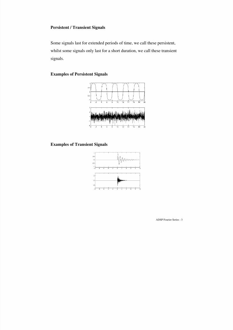
Persistent / Transient Signals

Some signals last for extended periods of time, we call these persistent,

whilst some signals only last for a short duration, we call these transient

signals.

Examples of Persistent Signals

Examples of Transient Signals




Deterministic / Random

Deterministic signals are completely predictable, e.g. there is an

underlying equation which defines the signal.

Random signals are unpredictable, in that you can not use past (or

future values) to exactly predict a data point.

On the previous slide the pictures of transient and persistent signals

and in both cases included one deterministic example and one random

example.

Below shows examples two more examples of random persistent

signals




DISCUSSION

The preceding signal descriptions contain some idealisations:

• No signal is truly persistent – it does not last forever.

• No measured signal is truly deterministic, when we measure a signal

some level of noise (randomness) is always present.

The ideas regarding signal types are models of reality.

We may consider the same signal using more than one model, for example:

Are heart sounds persistent or transient?

• Each individual beat is transient , consisting of a “lup” and a “dup”.

• Over a longer time scale, we consider many beats and choose to

model the signal as persistent .

• Over very long time scales each of us lives and dies, so the heart

sound starts and stops, so the signal is transient .

Whilst we talk of a signal “being of a particular type”, in practice weshould understand this as actually meaning “we model a signal as being of

a particular type over the time-scales of interest”.




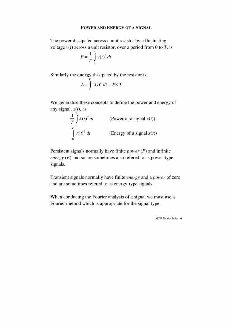
POWER AND ENERGY OF A SIGNAL

The power dissipated across a unit resistor by a fluctuatingvoltage v(t ) across a unit resistor, over a period from 0 to T , is

2

0

1( )

T

P v t dt T

= ∫

Similarly the energy dissipated by the resistor is

2

0

( )

T

E v t dt P T = = ×∫

We generalise these concepts to define the power and energy of

any signal, x(t ), as

2

0

1( )

T

t dt T ∫

(Power of a signal x(t ))

2

0

( )

T

x t dt ∫ (Energy of a signal x(t ))

Persistent signals normally have finite power (P) and infinite

energy ( E ) and so are sometimes also refered to as power-type

signals.

Transient signals normally have finite energy and a power of zero

and are sometimes refered to as energy-type signals.

When conductng the Fourier analysis of a signal we must use a

Fourier method which is appropriate for the signal type.




ENERGY-TYPE AND POWER-TYPE SIGNALS

For persistent signals, the concept of power is well-defined, but

energy is unbounded.

Specifically if x(t ) is persistent then for the energy:

2

0( ) as

T

x t dt T → ∞ → ∞∫

Whereas for the power we have:

2

0

1( ) as

T

x t dt P T T

→ → ∞∫

For transient signals, energy is well defined, but the power tends

to zero.

Specifically for a trasnient signal x(t ) the energy satisfies:

2

0

( ) as

T

x t dt E T → → ∞∫

Whereas:

2

0

1( ) 0 as

T

x t dt T T

→ → ∞∫




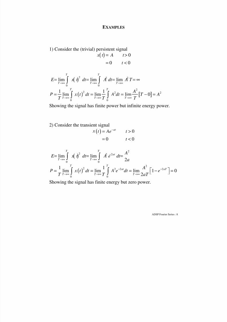
EXAMPLES

1) Consider the (trivial) persistent signal

( ) 0

0 0

x t A t

t

= >

= <

( )2 2 2

0 0

lim lim lim

T T

T T T E x t dt A dt A T →∞ →∞ →∞= = = = ∞∫ ∫

( ) [ ]2

2 2 2

0 0

1 1lim lim lim 0

T T

T T T

AP x t dt A dt T A

T T T →∞ →∞ →∞= = = − =∫ ∫

Showing the signal has finite power but infinite energy power.

2) Consider the transient signal

( ) 0

0 0

at t Ae t

t

−= >

= <

( )2

2 2 2

0 0

lim lim2

T T

at

T T

A E x t dt A e dt

a

−

→∞ →∞

= = =

∫ ∫

( )2

2 2 2 2

0 0

1 1lim lim lim 1 0

2

T T

at aT

T T T

AP x t dt A e dt e

T T aT

− −

→∞ →∞ →∞ = = = − = ∫ ∫

Showing the signal has finite energy but zero power.




DELTA FUNCTIONS

There are two distinct forms of delta function we shall employ.

1) Dirac delta function

We denote it δ(t ) and it is a function of continuous time t .

2) Kronecker delta function

We denote this δ(n) and it is a function of a discrete variable n.

The only difference in notation is the form of the argument

(potential this is confusing!) But the context should always make

it clear which function we are refering to.

The Kronecker delta is a simple sequence with useful properties,

specifically

( ) 0 0

1 0

n n

n

δ = ≠

= =

The Dirac delta is not so simple.




DIRAC DELTA FUNCTION

A Dirac delta function is a mathematical entity which can be

described as a perfect impulse.

Properties of a Dirac delta function, δ(t ):

1) δ(-t ) = δ(t ) Delta functions are symmetric.

2) ( ) 1t dt

∞

−∞

δ =∫

3) ( ) ( ) ( )2

1

1 2

L

L

x t t a dt x a L a Lδ − = < <∫

There is more than one definition of a delta function, but the most

common is

( ) ( )

( )

0

1/ for / 2 / 2

0 otherwise

Limt R t

R t t

ε

ε

δ =ε →

= ε − ε < < ε

=




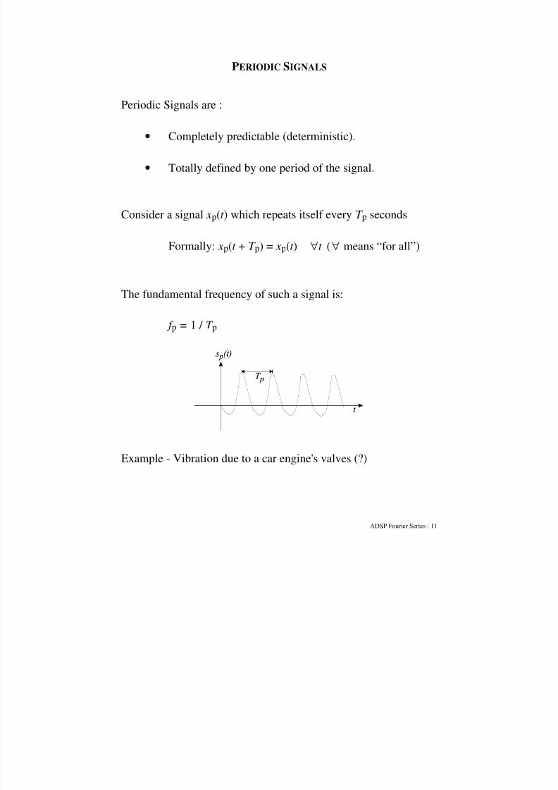
PERIODIC SIGNALS

Periodic Signals are :

• Completely predictable (deterministic).

• Totally defined by one period of the signal.

Consider a signal xp(t ) which repeats itself every T p seconds

Formally: xp(t + T p) = xp(t ) t ∀ (∀ means “for all”)

The fundamental frequency of such a signal is:

f p = 1 / T p

Example - Vibration due to a car engine's valves (?)




EXAMPLES OF PERIODIC SIGNALS

Sine Wave

(Fundamental Frequency 1 Hz)

Sine Wave


Square Wave


Triangular Wave





EXAMPLES OF PERIODIC SIGNALS (?)

Sine Wave


Sine Wave

(Fundamental Frequency 1.25 Hz)

Sum of 2 Sine Waves

(Frequencies 1 & 1.25 Hz)

Sum of 2 Sine Waves

(Frequencies 1 & √2 Hz)

Repeats every 4 seconds Never repeats – not periodic




MORE EXAMPLES OF PERIODIC SIGNALS (?)

Sine Wave plus Noise


Frequency Modulated Signal

(2 Hz with a 0.2 Hz Modulation)

Noise means it does not exactly repeat

itself

Repeats itself every 5 s

Modulate Noise

(Modulation Frequency .25 Hz) Frequency Modulation

(√2 modulated by 0.2 Hz)

Has a periodic structure, Does not repeat itself

but does not repeat itself.




PSEUDO-PERIODIC SIGNALS

Some real world signals are nearly periodic and can be usefully

analysed as if they were exactly periodic.

Such signals are sometimes refered to as pseudo-periodic signals.

Example: Voiced Speech {/ou/ as in ‘about’}




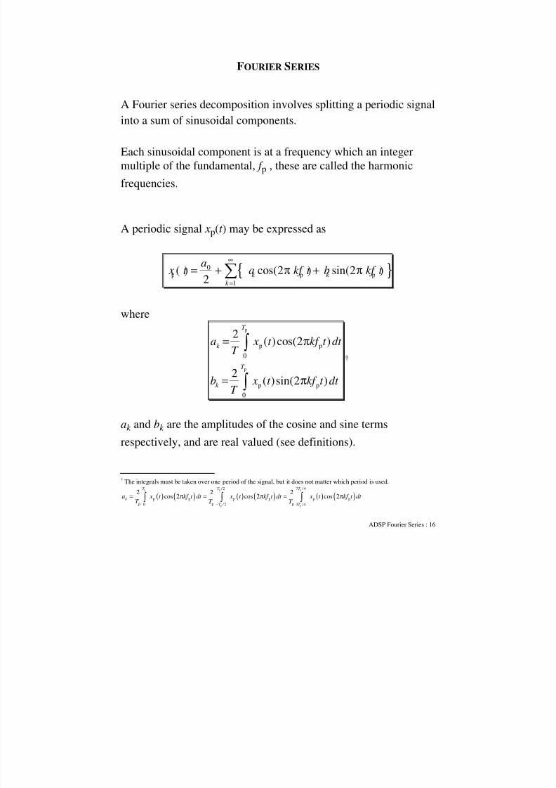
FOURIER SERIES

A Fourier series decomposition involves splitting a periodic signal

into a sum of sinusoidal components.

Each sinusoidal component is at a frequency which an integer

multiple of the fundamental, f p , these are called the harmonic

frequencies.

A periodic signal xp(t ) may be expressed as

{ }0p p p

1

( ) cos(2 ) sin(2 )2

k k

k

a x t a kf t b kf t

∞

=

= + π + π∑

where

p

p

p p

0

p p

0

2( )cos(2 )

2( )sin(2 )

T

k

T

k

a x t kf t dt T

b x t kf t dt

T

= π

= π

∫

∫

†

ak and bk are the amplitudes of the cosine and sine terms

respectively, and are real valued (see definitions).

†The integrals must be taken over one period of the signal, but it does not matter which period is used.

( ) ( ) ( ) ( ) ( ) ( )p p p

p p

/2 7 /4

p p p p p p

p p p0 /2 3 / 4

2 2 2cos cos cos

T T T

k

T T

a x t kf t dt x t kf t dt x t kf t dt T T T −

= 2π = 2π = 2π∫ ∫ ∫




EXAMPLES OF FOURIER SERIES

The Square Wave:

p p

1

4( ) sin(2 (2 1) )

(2 1)k

x t k f t k

∞

=

= π −π −∑

i.e. 4

k a

k =

π for k odd and ak = 0 for k even. bk = 0 for all k .

Triangular Wave :

p p2 21

8( ) cos(2 (2 1) )

(2 1)k

t k f t k

∞

=

= π −π −∑

i.e.

2 2

8k a k = π for n odd and ak = 0 for k even. bk = 0 for all k .



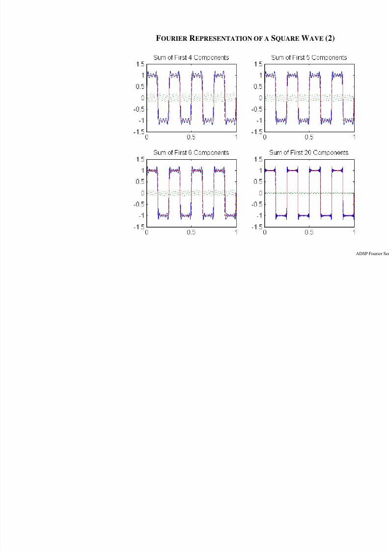
FOURIER REPRESENTATION OF A SQUARE WAVE



FOURIER REPRESENTATION OF A SQUARE WAVE (2




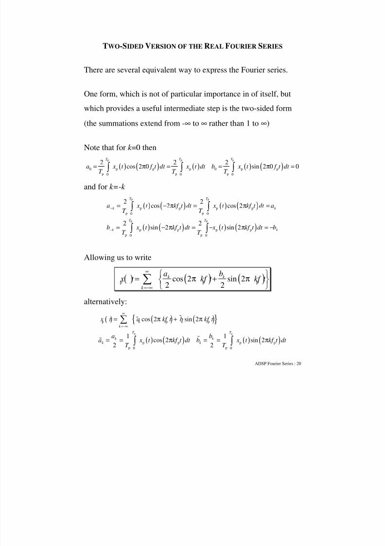
TWO-SIDED VERSION OF THE REAL FOURIER SERIES

There are several equivalent way to express the Fourier series.

One form, which is not of particular importance in of itself, but

which provides a useful intermediate step is the two-sided form

(the summations extend from -∞ to ∞ rather than 1 to ∞)

Note that for k =0 then

( ) ( ) ( ) ( ) ( )P P P

0 p p p 0 p p

p p p0 0 0

2 2 2cos 2 0 sin 2 0 0

T T T

a x t f t dt x t dt b x t f t dt T T T

= π = = π =∫ ∫ ∫

and for k=-k

( ) ( ) ( ) ( )

( ) ( ) ( ) ( )

P P

P P

p p p p

p p0 0

p p p p

p p0 0

2 2cos 2 cos 2

2 2sin 2 sin 2

T T

k k

T T

k k

a x t kf t dt x t kf t dt aT T

b x t kf t dt x t kf t dt bT T

−

−

= − π = π =

= − π = − π = −

∫ ∫

∫ ∫

Allowing us to write

( ) ( ) ( )p p pcos 2 sin 22 2

k k

k

a b x t kf t kf t

∞

=−∞

= π + π

∑

alternatively:

( ) ( ) ( ){ }

( ) ( ) ( ) ( )p p

p p p

p p p p

p p0 0

cos 2 sin 2

1 1cos 2 sin 22 2

k k

k

T T

k k k k

x t a kf t b kf t

a ba x t kf t dt b x t kf t dt T T

∞

=−∞

= π + π

= = π = = π

∑

∫ ∫




AMPLITUDE AND PHASE VERSION OF THE REAL FOURIER

SERIES

The simple Fourier Series :

{ }0p p p

1

( ) cos(2 ) sin(2 )2

k k

k

a x t a kf t b kf t

∞

=

= + π + π∑

Can be written as the summation of a single cosine (or sine) term:0

p p

1

( ) cos(2 )2

k k

k

c x t c kf t

∞

=

= + π − φ∑

This is a simple manipulation of the classical Fourier Series

expansion.

The ck and φk can be found by evaluating ak and bk then using the

relationships

2 2 1; tan k

k k k k

k

bc a b

a

− = + φ =

ck 2 /2 represents the power of the signal contained in the k th

harmonic.




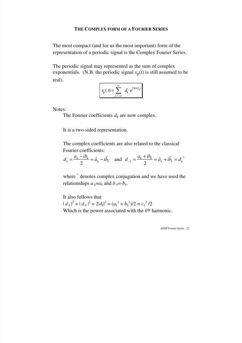
THE COMPLEX FORM OF A FOURIER SERIES

The most compact (and for us the most important) form of the

representation of a periodic signal is the Complex Fourier Series.

The periodic signal may represented as the sum of complex

exponentials. (N.B. the periodic signal xp(t ) is still assumed to be

real).

p2

p ( )ikf t

k

k

x t d e∞ π

=−∞

= ∑

Notes:

The Fourier coefficients d k are now complex.

It is a two-sided representation.

The complex coefficients are also related to the classical

Fourier coefficients:

2

k k k k k

a ibd a ib

−= = − and

*

2

k k k k k k

a ibd a ib d −

+= = + =

where * denotes complex conjugation and we have used the

relationships a-k =ak and b-k =-bk .

It also follows that

| d k |2 + | d -k |

2 = 2|d k |2 = (ak

2 + bk 2)/2 = ck

2 /2

Which is the power associated with the k th

harmonic.




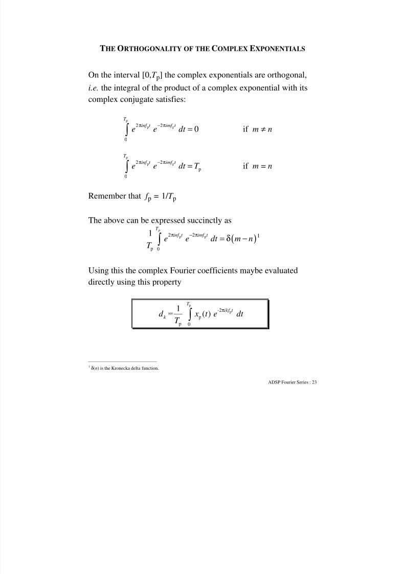
THE ORTHOGONALITY OF THE COMPLEX EXPONENTIALS

On the interval [0,T p] the complex exponentials are orthogonal,

i.e. the integral of the product of a complex exponential with its

complex conjugate satisfies:

p

p p2 2

0

0

T

inf t imf t e e dt

π − π =∫ if m ≠ n

p

p p2 2

p

0

T

inf t imf t e e dt T

π − π =∫ if m = n

Remember that f p = 1/ T p

The above can be expressed succinctly as

( )p p2 2

p 0

1pT

inf t imf t e e dt m n

T

π − π = δ −∫ 1

Using this the complex Fourier coefficients maybe evaluated

directly using this property

p

p-2

p

p 0

1( )

T

ikf t

k d x t e dt

T

π= ∫

1 δ(n) is the Kronecka delta function.




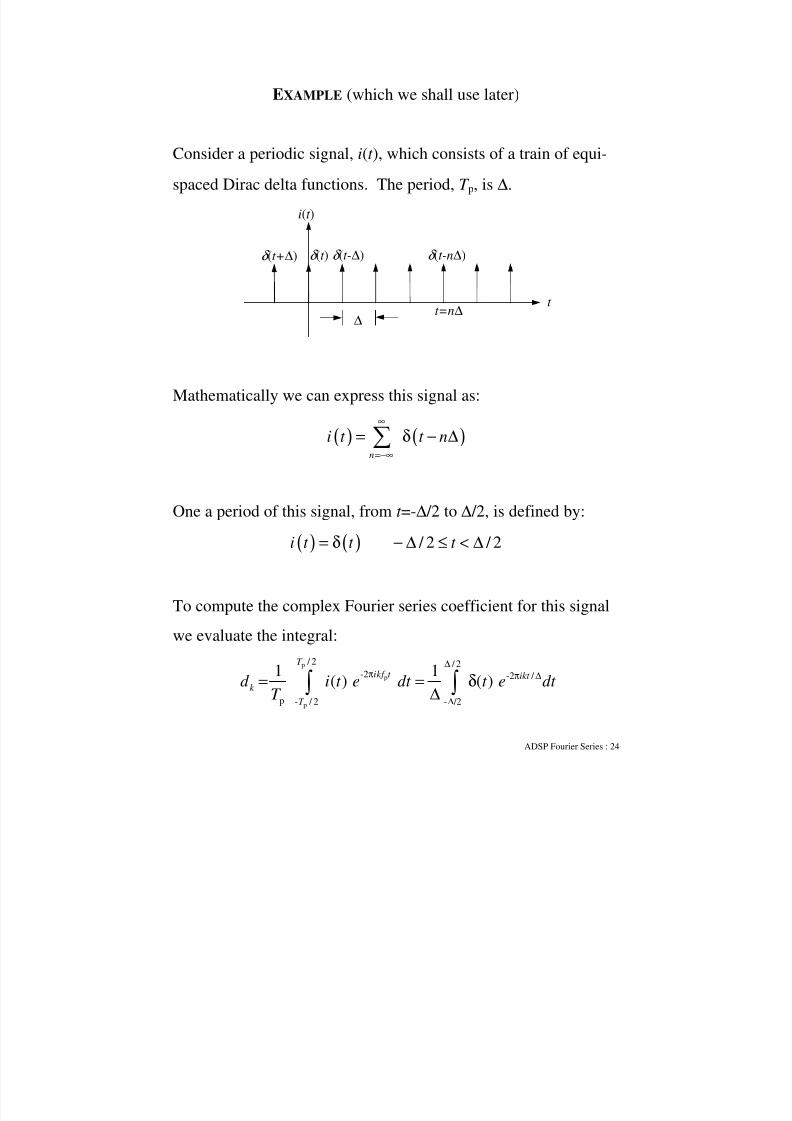
EXAMPLE (which we shall use later)

Consider a periodic signal, i(t ), which consists of a train of equi-

spaced Dirac delta functions. The period, T p, is ∆.

i(t )

∆

δ (t ) δ (t-∆)

t

δ (t-n∆)

t=n∆

δ (t+∆)

Mathematically we can express this signal as:

( ) ( )n

i t t n∞

=−∞

= δ − ∆∑

One a period of this signal, from t =-∆ /2 to ∆ /2, is defined by:

( ) ( ) / 2 / 2i t t t = δ − ∆ ≤ < ∆

To compute the complex Fourier series coefficient for this signal

we evaluate the integral:

p

p

p

/ 2 / 2-2 -2 /

p - / 2 - /2

1 1( ) ( )

T

ikf t ikt

k

T

d i t e dt t e dt T

∆π π ∆

∆

= = δ∆∫ ∫




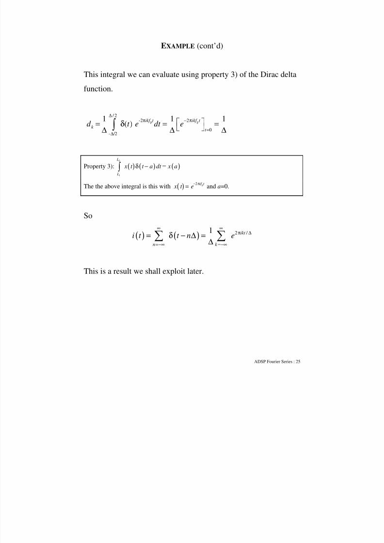
EXAMPLE (cont’d)

This integral we can evaluate using property 3) of the Dirac delta

function.

p p

/ 2-2 2

0

- /2

1 1 1( )

ikf t ikf t

k t

d t e dt e

∆π − π

=

∆

= δ = =

∆ ∆ ∆

∫

Property 3): ( ) ( ) ( )2

1

L

L

x t t a dt x aδ − =∫

The the above integral is this with ( ) p2 if t x t e

− π= and a=0.

So

( ) ( ) 2 / 1 ikt

n k

i t t n e∞ ∞

π ∆

=−∞ =−∞

= δ − ∆ =∆∑ ∑

This is a result we shall exploit later.




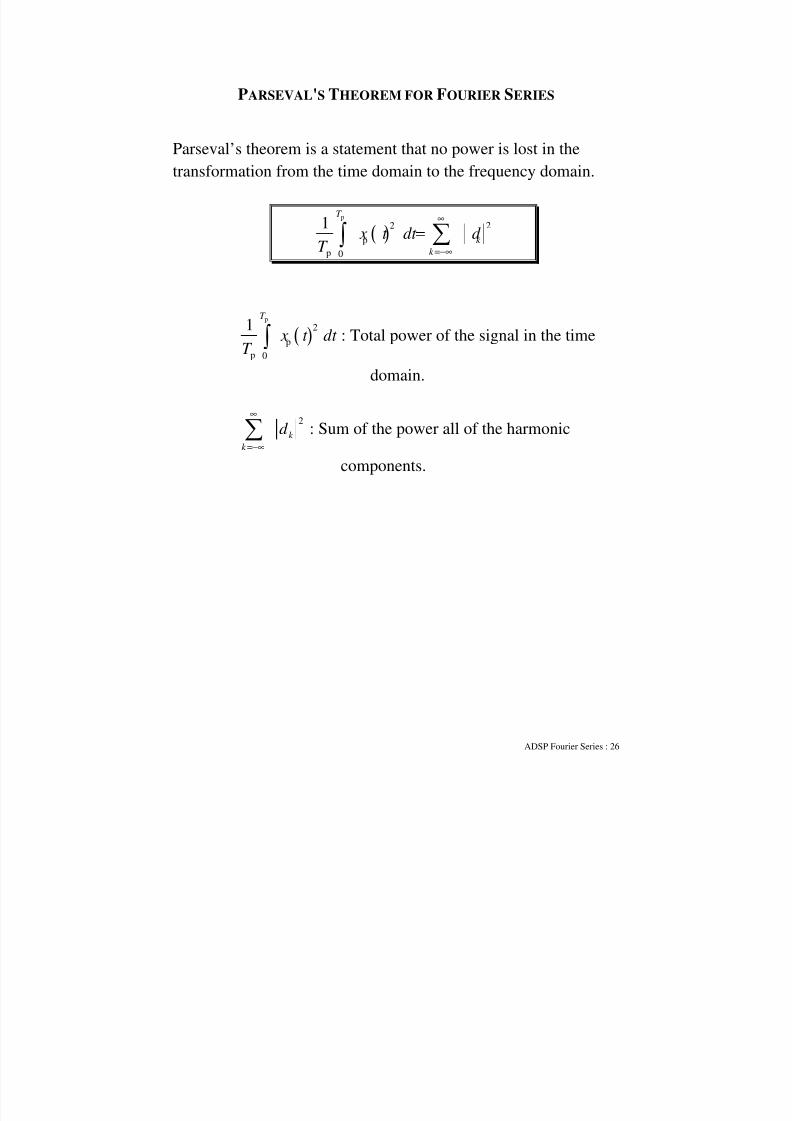
PARSEVAL'S THEOREM FOR FOURIER SERIES

Parseval’s theorem is a statement that no power is lost in the

transformation from the time domain to the frequency domain.

( )p

22

p

p 0

1T

k

k

x t dt d T

∞

=−∞

= ∑∫

( )p

2

p

p 0

1T

x t dt T ∫ : Total power of the signal in the time

domain.

2

k

k

d ∞

=−∞∑ : Sum of the power all of the harmonic

components.




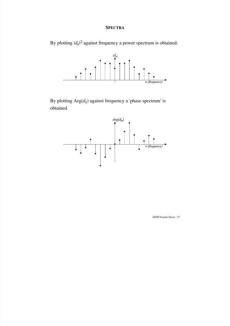
SPECTRA

By plotting |d k |2 against frequency a power spectrum is obtained.

By plotting Arg(d k ) against frequency a 'phase spectrum' is

obtained.




DIRICHLET CONDITIONS

The partial sums of the Fourier Series will converge (in the mean

square sense) to the true signal assuming all of the following

(Dirichlet) conditions are met:

1) The signal is absolutely integrable, i.e.

( )p

2

p

p 0

1T

x t dt T

< ∞∫

Example that fails: xp(t )=1/ t , 0≤t <1.

2) The signal has bounded variation, i.e. there are a finite number

of maxima/minima during any period.

Example that fails:2

sin t

π

, 0≤t <1, (the frequency tends to

infinity as t tends to 0.)

3) The can only be a finite number of discontinuities within a

period.




Exercises

1) For the following signals decide if they are persistent or transient and compute their energies and

powers:

a)( ) 0

0 0

t x t e t

t

−= ≥

= <

b) ( ) ( )sin x t A t = ω

c)( ) ( )cos 0, 0

0 0

t x t e t t

t

−α= ω ≥ α >

= <

2) Show that the Fourier series coefficients of the square wave, one period of which is defined by:

( ) 0 0.5

0.5 1

x t A t

A t

= < <

= − < <

are given by:

( )( )1 1k

k d ik

− −=

π

3) Show that if ( ) x t has the Fourier series 2 / pikt T k

k

d e∞

π

=−∞∑ then the Fourier series coefficients of its

derivative, ( )' x t , are given by2

k

p

d ik

T

π.

4) Prove the orthogonality of the sines and cossine functions over the interval [0,T p], i.e. show:

( ) ( )

( ) ( ) ( ) ( )

( ) ( ) ( ) ( )

P

P P

P P

p p

0

p

p p p p0 0

p

p p p p

0 0

sin 2 cos 2 0 ,

cos 2 cos 2 0 cos 2 cos 22

sin 2 sin 2 0 sin 2 sin 22

T

T T

T T

mf t nf t dt m n

T mf t nf t dt m n mf t nf t dt m n

T mf t nf t dt m n mf t nf t dt m n

π π = ∀

π π = ≠ π π = =

π π = ≠ π π = =

∫

∫ ∫

∫ ∫

Use this to prove the basic Fourier series representation, namely given that

{ }0p p p

1

( ) cos(2 ) sin(2 )2

k k

k

a x t a kf t b kf t

∞

=

= + π + π∑ then

p p

p p p p

0 0

2 2( )cos(2 ) ( )sin(2 )

T T

k k a x t kf t dt b x t kf t dt T T

= π = π∫ ∫



5) Use the orthogonality of the complex exponentials to show that given p2

p( )ikf t

k

k

x t d e∞

π

=−∞

= ∑ then

p

p-2

pp 0

1

( )

T

ikf t

k d x t e dt T

π

= ∫ .

6) Show that the conventional Fourier series can be written as 0p p

1

( ) cos(2 )2

k k

k

c x t c kf t

∞

=

= + π − φ∑

where2 2

k k k c a b= + and ( )1tan / k k k b a

−φ = .

7) Prove that if nd are the complex Fourier coefficients of the signal xp(t ), then the Fourier

coefficeints of xp(t -τ) are given by p2 if

ne d − π τ

.

Hence prove that if the periodic signal is delayed by an integer number of periods,p

q

T τ = then the

complex Fourier coefficients are unchanged.

8) Prove Parseval’s theorem ( )p

2 2

p

p 0

1T

k

k

x t dt d T

∞

=−∞

= ∑∫

9) Prove the Fourier series on Slide 20 is equivalent to the conventional Fourier series

representation.

Date post:	10-Apr-2018
Category:	Documents
Upload:	mcenrrou
View:	217 times
Download:	0 times

Fourier Series 2009

Documents