82
Fourier Transform and Image Filtering CS/BIOEN 6640 Lecture Marcel Prastawa Fall 2010
| Date post: | 25-Apr-2018 |
| Category: |
Documents |
| Upload: | duongtuyen |
| View: | 219 times |
| Download: | 1 times |
Fourier Transform and
Image Filtering
CS/BIOEN 6640Lecture Marcel Prastawa
Fall 2010
The Fourier Transform
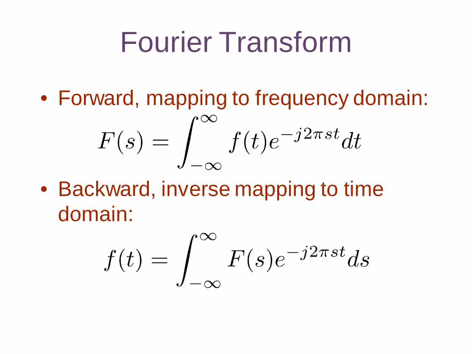
Fourier Transform
• Forward, mapping to frequency domain:
• Backward, inverse mapping to time domain:
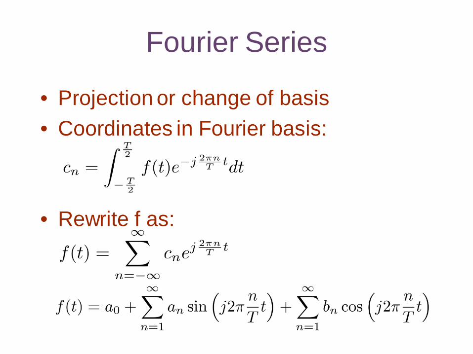
Fourier Series
• Projection or change of basis• Coordinates in Fourier basis:
• Rewrite f as:
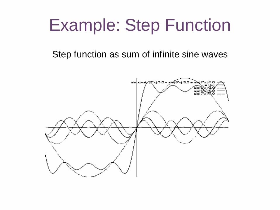
Example: Step FunctionStep function as sum of infinite sine waves
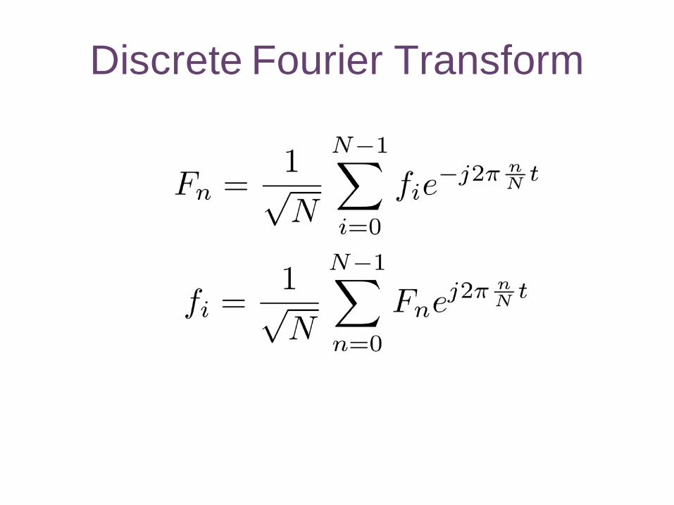
Discrete Fourier Transform
Fourier Basis
• Why Fourier basis?
• Orthonormal in [-pi, pi]• Periodic• Continuous, differentiable basis
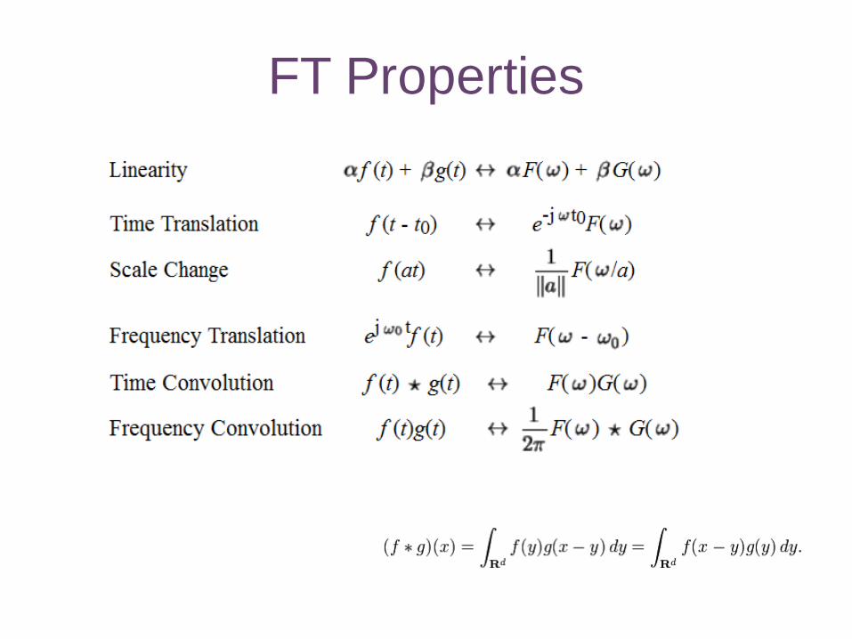
FT Properties
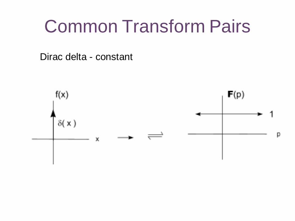
Common Transform PairsDirac delta - constant
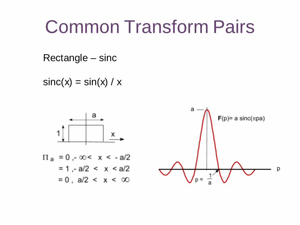
Common Transform PairsRectangle – sinc
sinc(x) = sin(x) / x
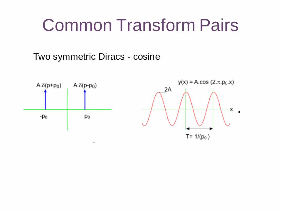
Common Transform PairsTwo symmetric Diracs - cosine
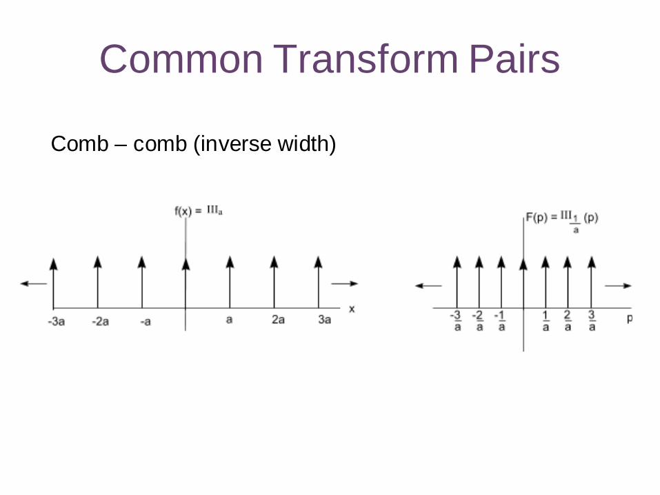
Common Transform Pairs
Comb – comb (inverse width)
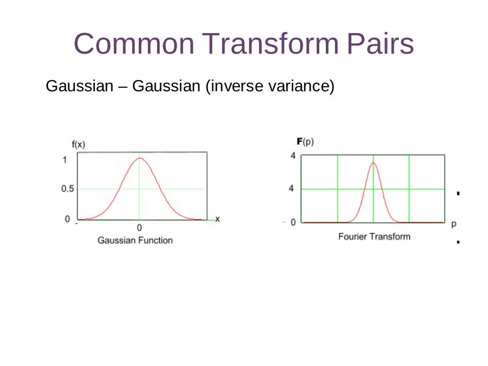
Common Transform PairsGaussian – Gaussian (inverse variance)
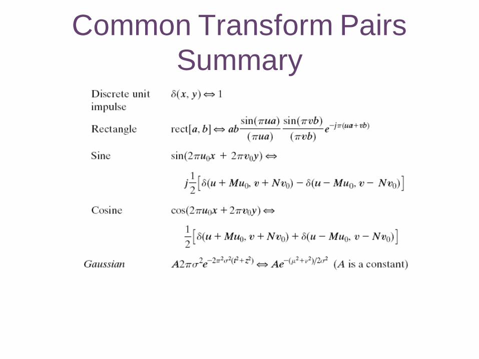
Common Transform Pairs Summary
Quiz
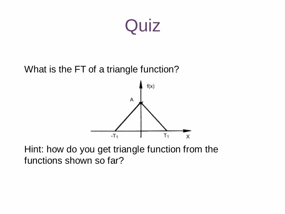
What is the FT of a triangle function?
Hint: how do you get triangle function from the functions shown so far?
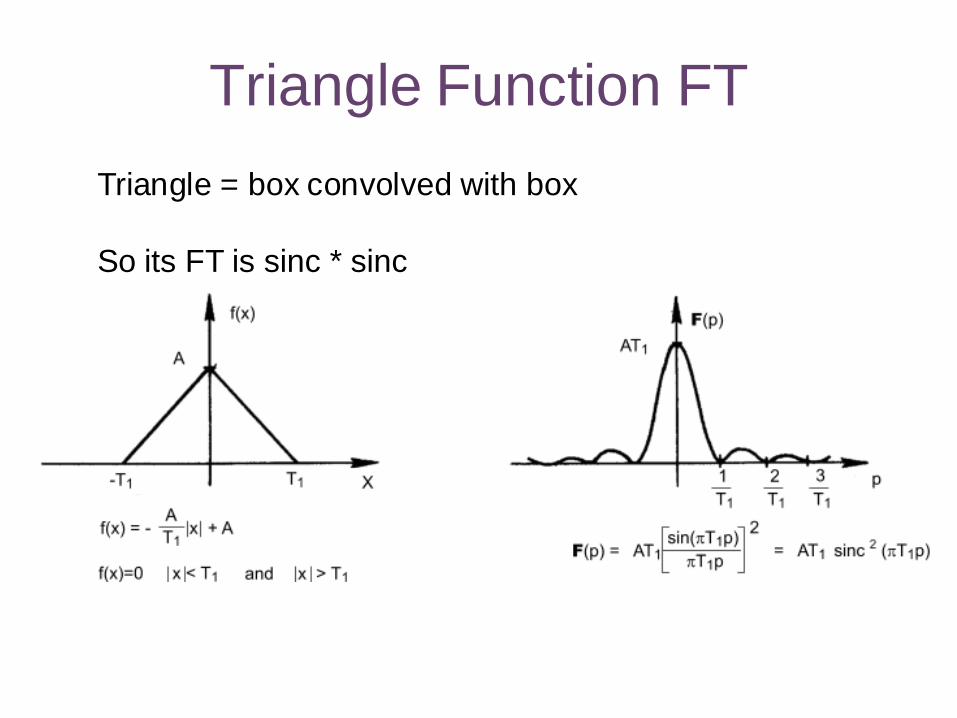
Triangle Function FTTriangle = box convolved with box
So its FT is sinc * sinc
Fourier Transform of Images
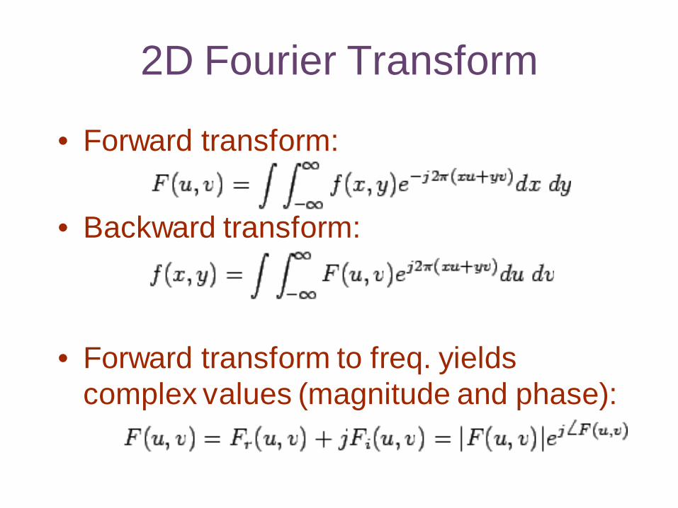
• Forward transform:
• Backward transform:
• Forward transform to freq. yields complex values (magnitude and phase):
2D Fourier Transform
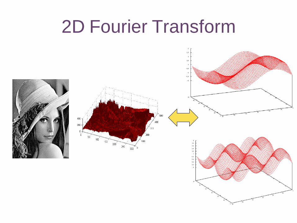
2D Fourier Transform
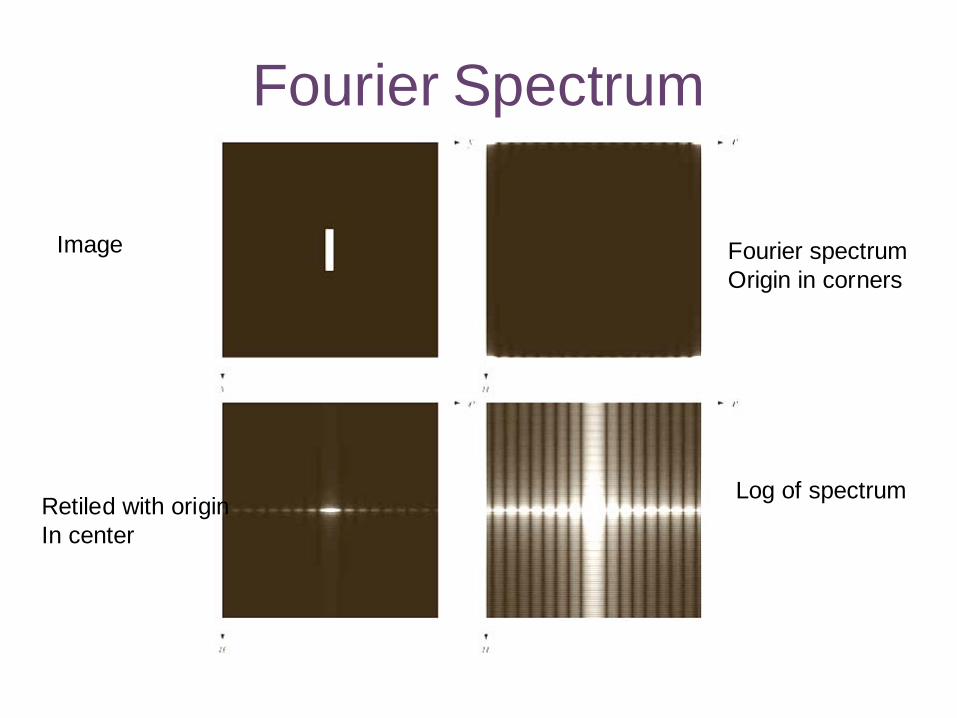
Fourier Spectrum
Fourier spectrumOrigin in corners
Retiled with originIn center
Log of spectrum
Image
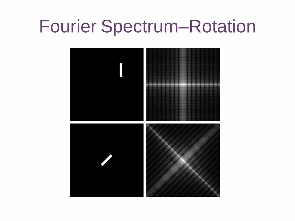
Fourier Spectrum–Rotation
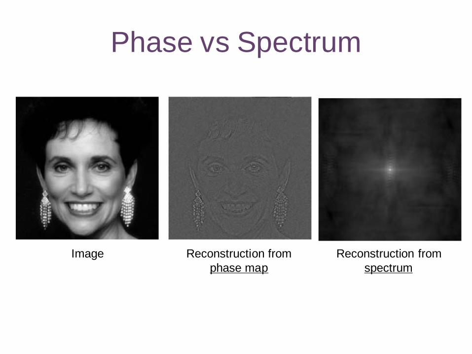
Phase vs Spectrum
Image Reconstruction fromphase map
Reconstruction fromspectrum
Fourier Spectrum Demo
http://bigwww.epfl.ch/demo/basisfft/demo.html
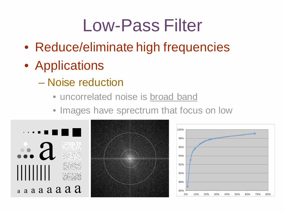
Low-Pass Filter• Reduce/eliminate high frequencies• Applications
– Noise reduction• uncorrelated noise is broad band• Images have sprectrum that focus on low
frequencies
86%
88%
90%
92%
94%
96%
98%
100%
0% 10% 20% 30% 40% 50% 60% 70% 80%
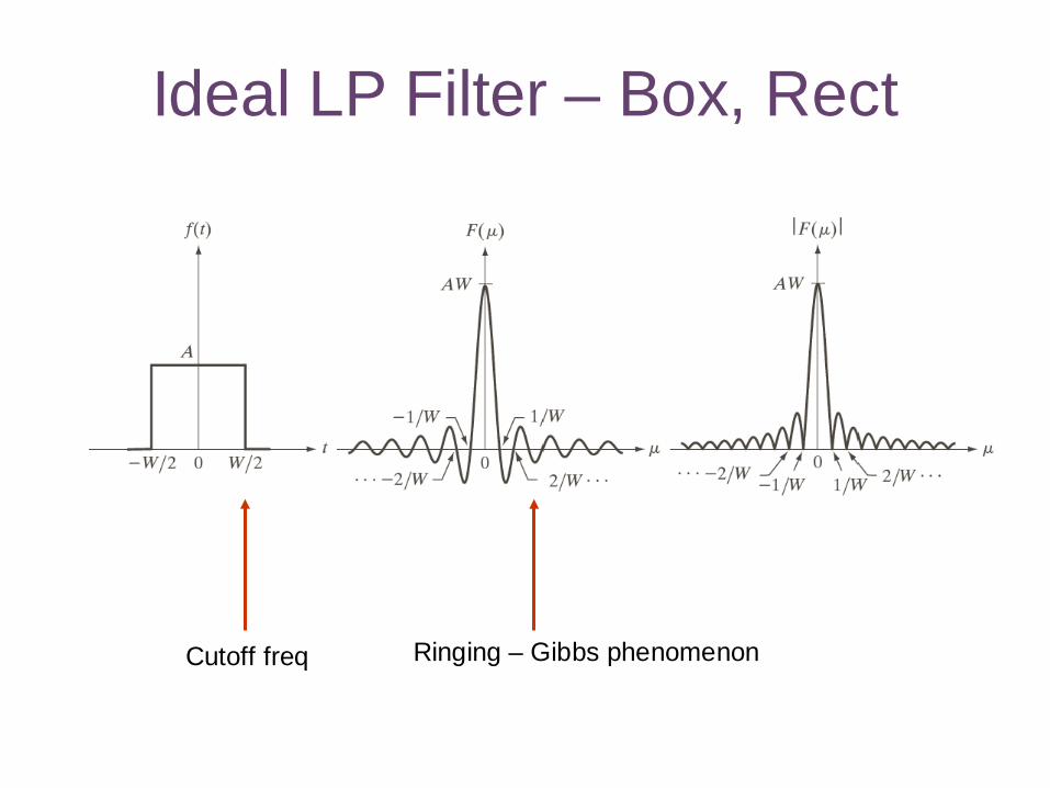
Ideal LP Filter – Box, Rect
Cutoff freq Ringing – Gibbs phenomenon
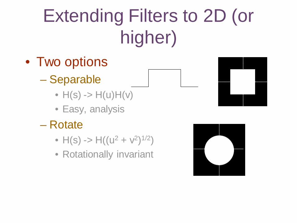
Extending Filters to 2D (or higher)
• Two options– Separable
• H(s) -> H(u)H(v)• Easy, analysis
– Rotate• H(s) -> H((u2 + v2)1/2)• Rotationally invariant
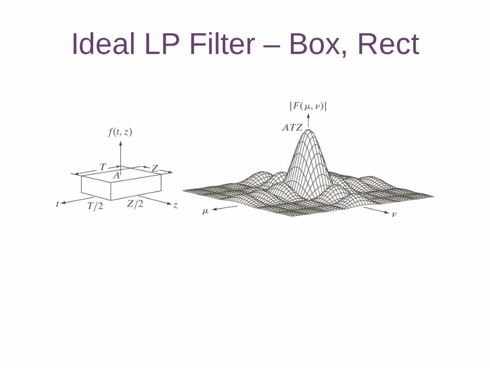
Ideal LP Filter – Box, Rect
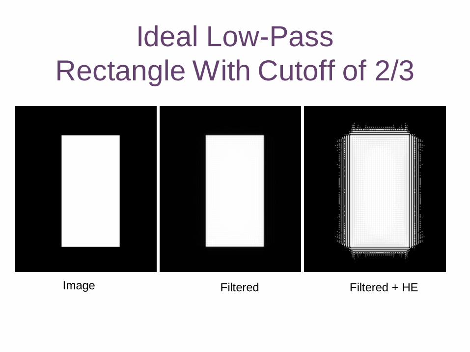
Ideal Low-Pass Rectangle With Cutoff of 2/3
Image Filtered Filtered + HE

Ideal LP – 1/3
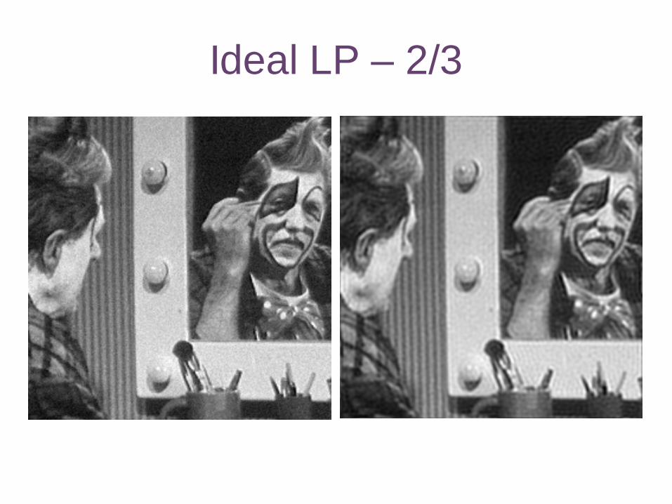
Ideal LP – 2/3
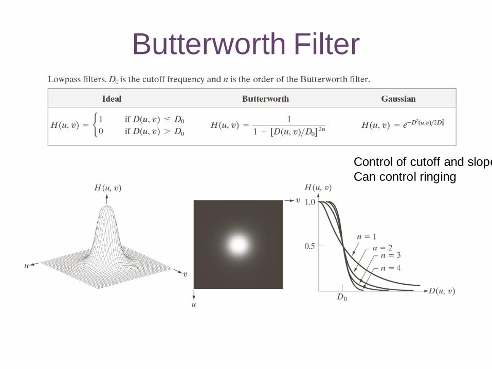
Butterworth Filter
Control of cutoff and slopeCan control ringing
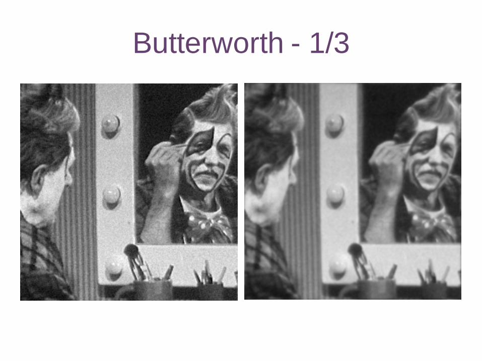
Butterworth - 1/3
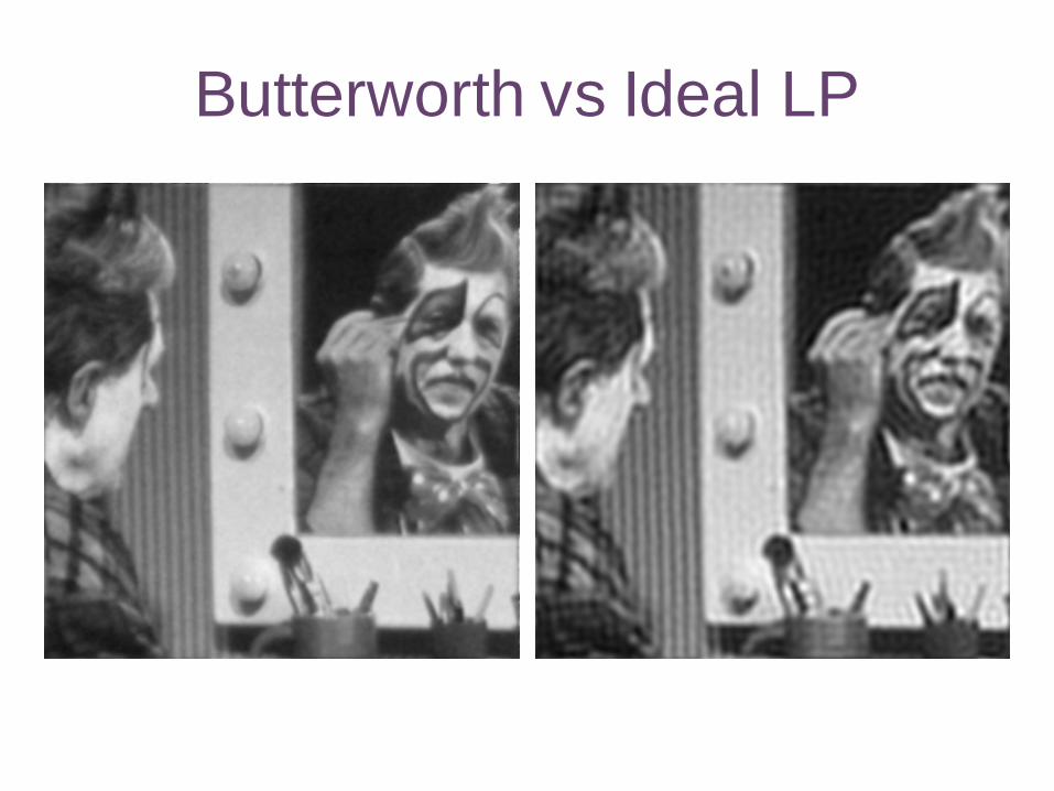
Butterworth vs Ideal LP
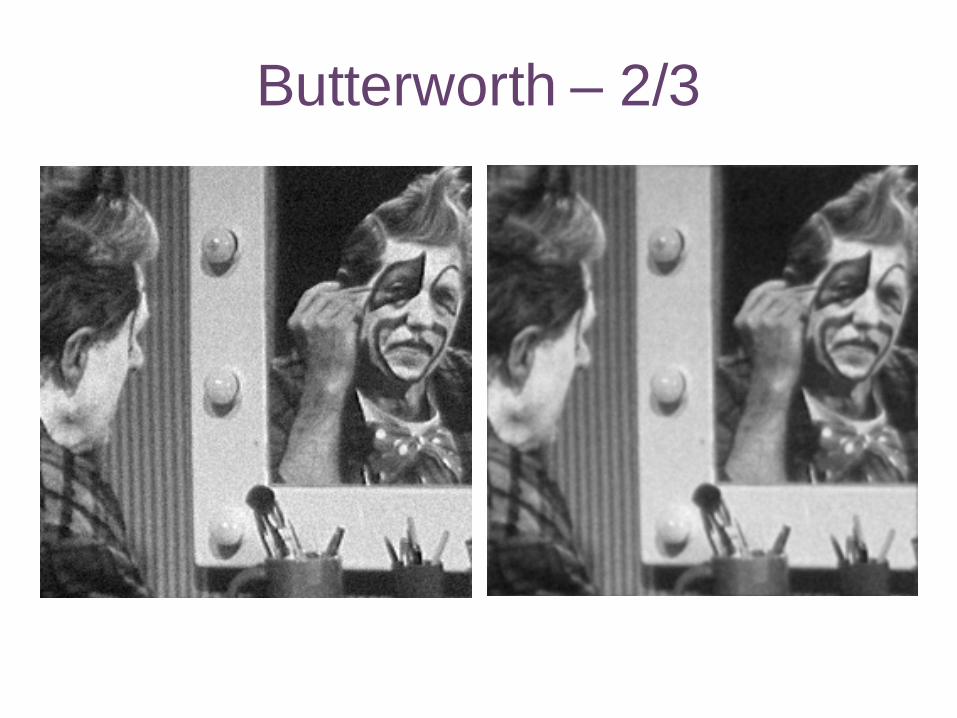
Butterworth – 2/3
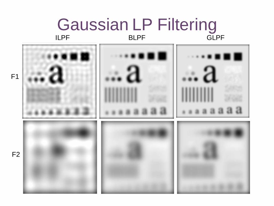
Gaussian LP FilteringILPF BLPF GLPF
F1
F2
High Pass Filtering
• HP = 1 - LP– All the same filters as HP apply
• Applications– Visualization of high-freq data (accentuate)
• High boost filtering– HB = (1- a) + a(1 - LP) = 1 - a*LP
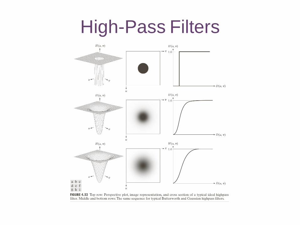
High-Pass Filters
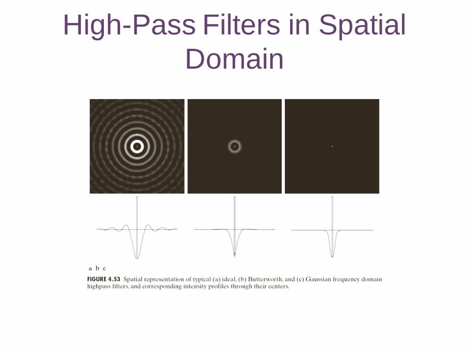
High-Pass Filters in Spatial Domain
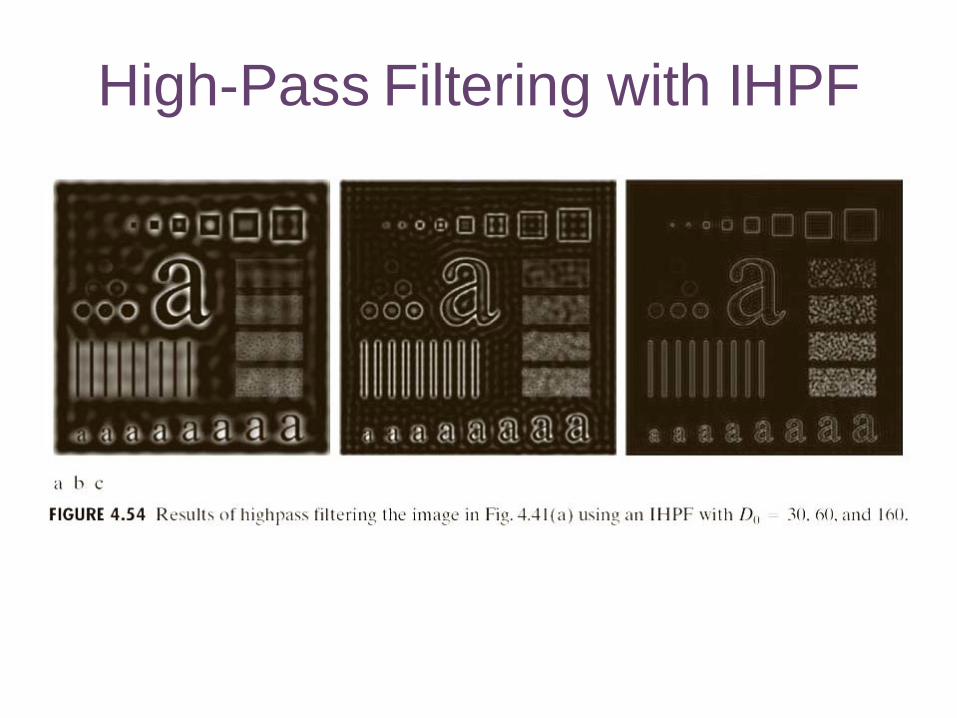
High-Pass Filtering with IHPF
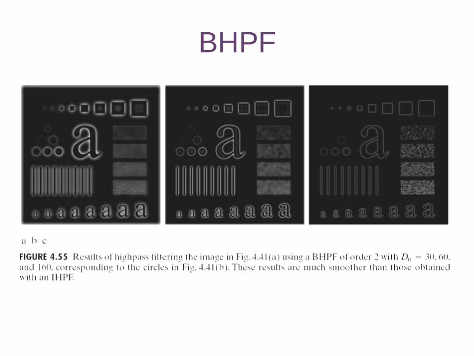
BHPF
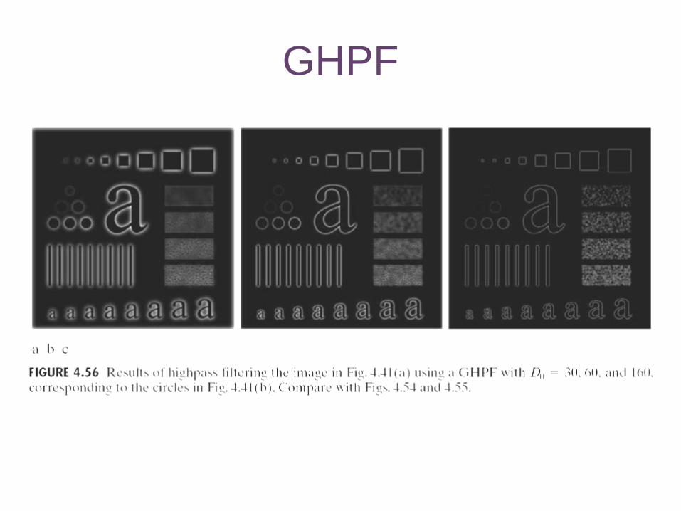
GHPF
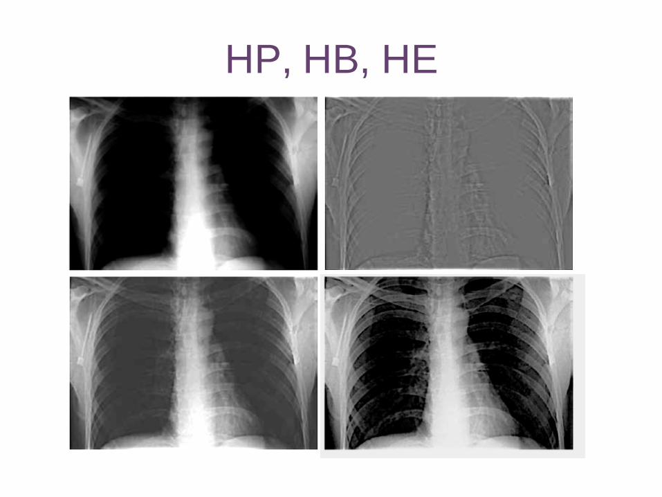
HP, HB, HE
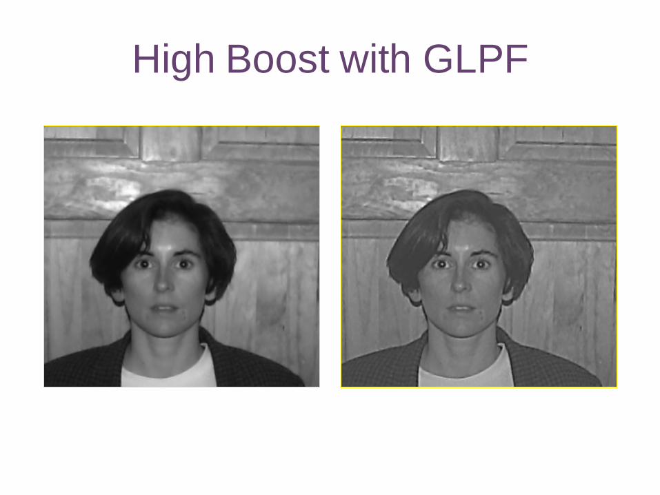
High Boost with GLPF

High-Boost Filtering
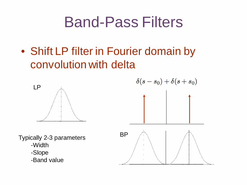
Band-Pass Filters
• Shift LP filter in Fourier domain by convolution with delta
LP
BPTypically 2-3 parameters-Width-Slope-Band value
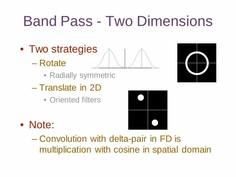
Band Pass - Two Dimensions
• Two strategies– Rotate
• Radially symmetric– Translate in 2D
• Oriented filters
• Note:– Convolution with delta-pair in FD is
multiplication with cosine in spatial domain
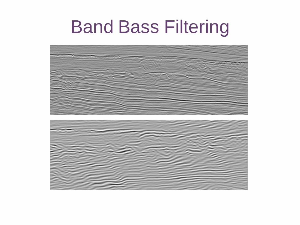
Band Bass Filtering
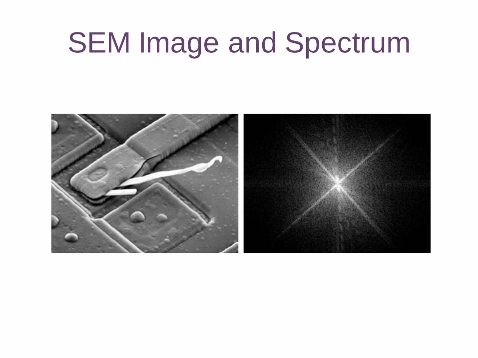
SEM Image and Spectrum
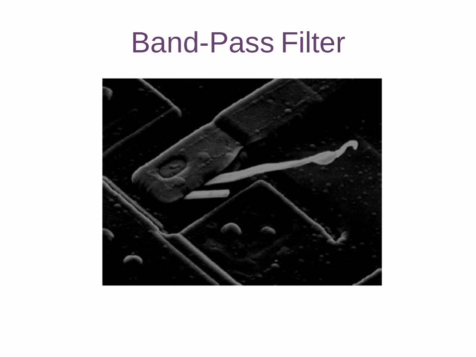
Band-Pass Filter
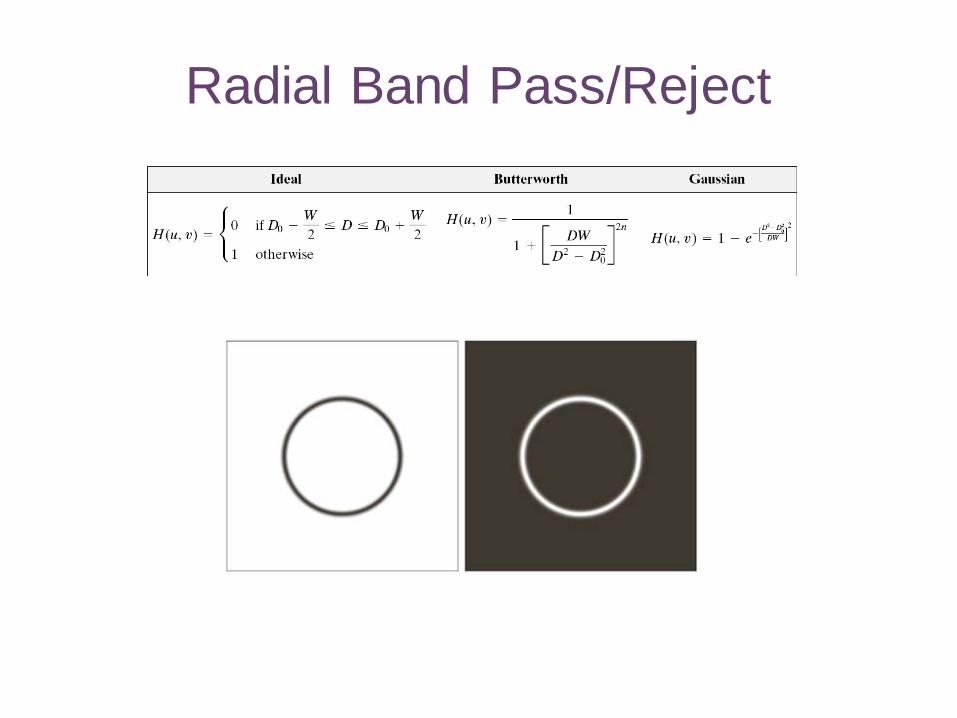
Radial Band Pass/Reject
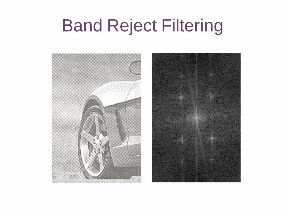
Band Reject Filtering
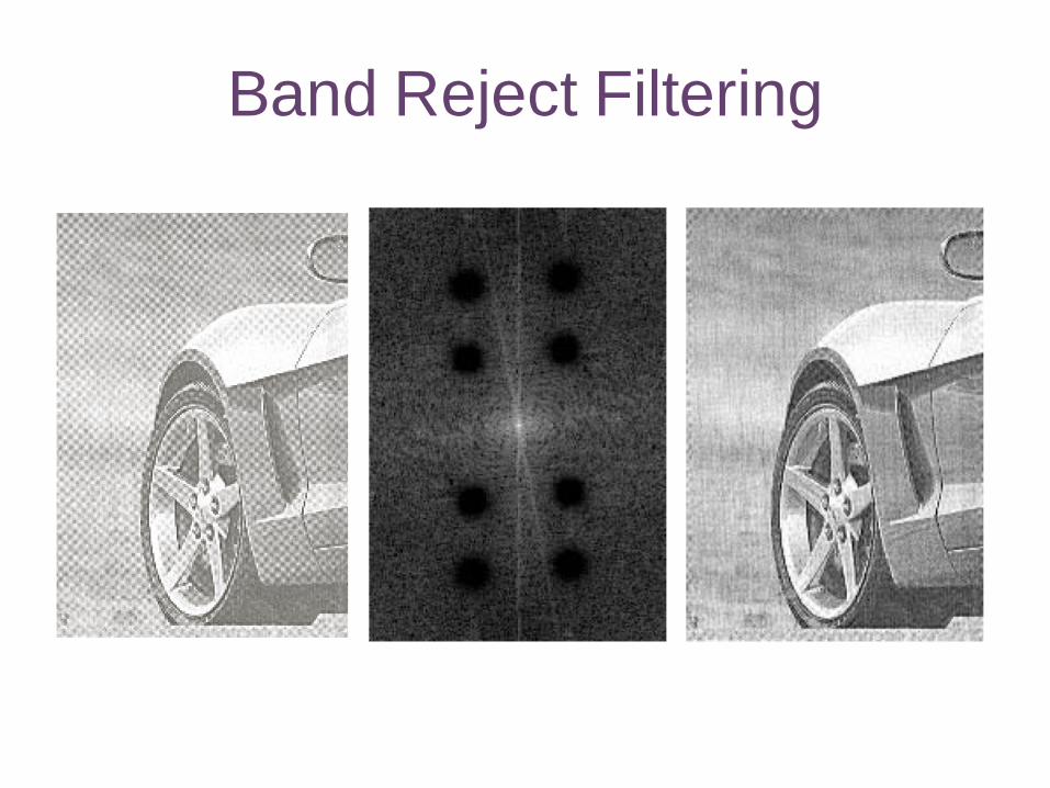
Band Reject Filtering
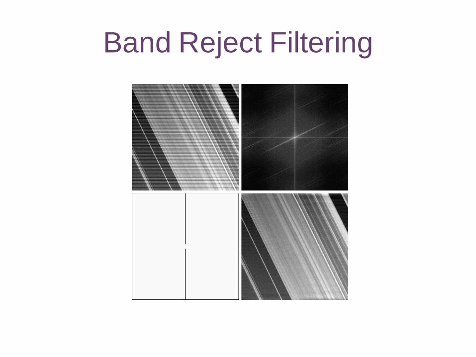
Band Reject Filtering

Aliasing
Discrete Sampling and Aliasing
• Digital signals and images are discrete representations of the real world – Which is continuous
• What happens to signals/images when we sample them?– Can we quantify the effects? – Can we understand the artifacts and can we limit
them?– Can we reconstruct the original image from the
discrete data?
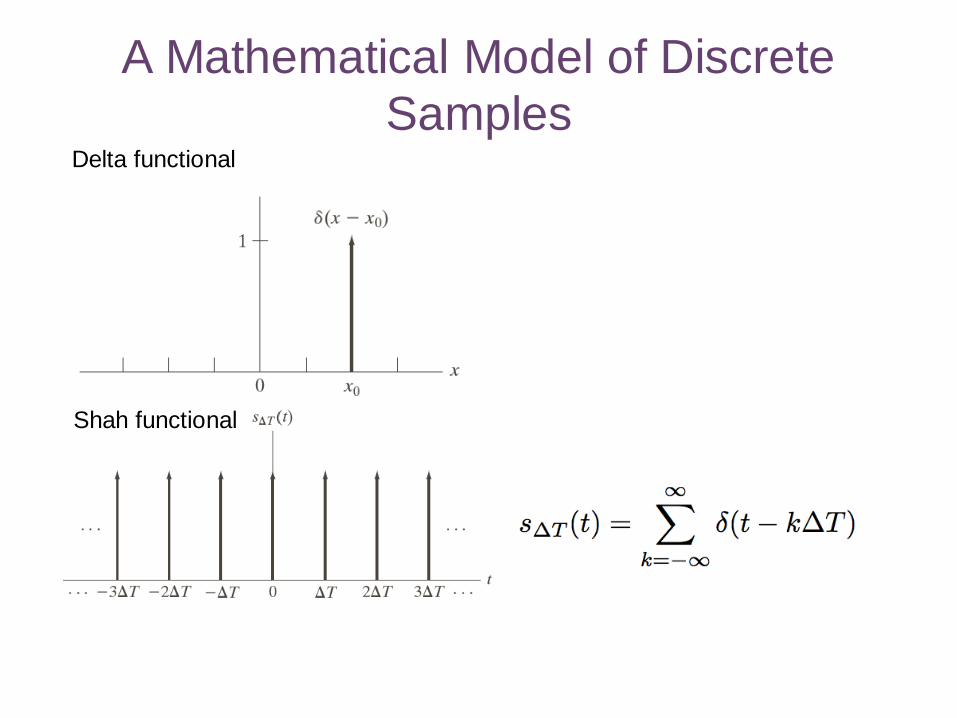
A Mathematical Model of Discrete Samples
Delta functional
Shah functional
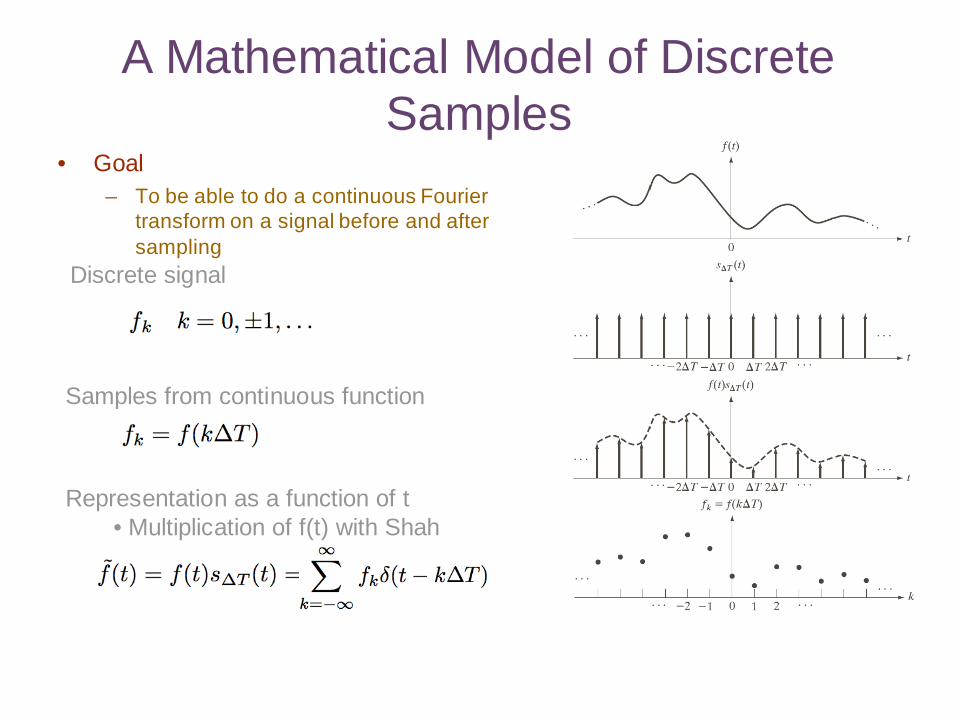
A Mathematical Model of Discrete Samples
Discrete signal
Samples from continuous function
Representation as a function of t• Multiplication of f(t) with Shah
• Goal– To be able to do a continuous Fourier
transform on a signal before and after sampling
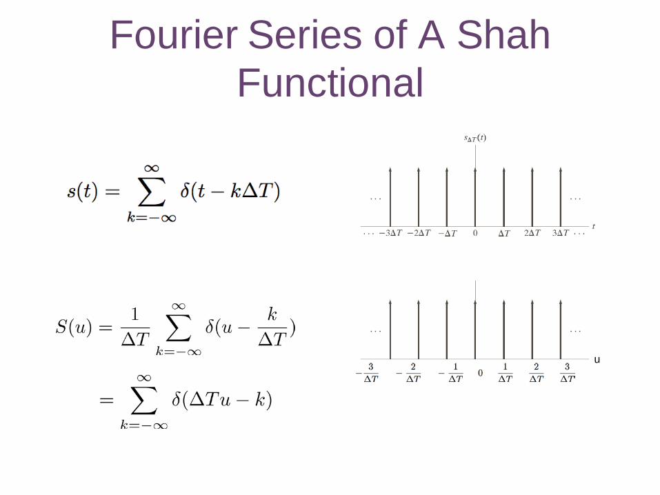
Fourier Series of A Shah Functional
u
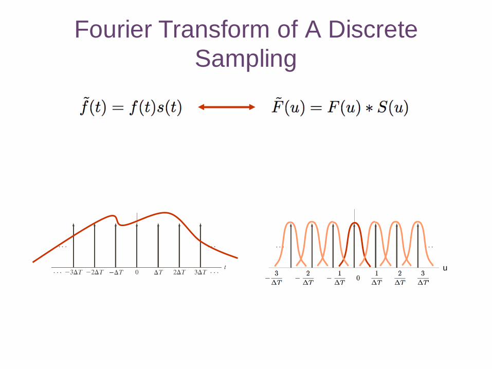
Fourier Transform of A Discrete Sampling
u

Fourier Transform of A Discrete Sampling
u
Energy from higher freqs gets folded back down into lower freqs –Aliasing
Frequencies get mixed. The original signal is not recoverable.
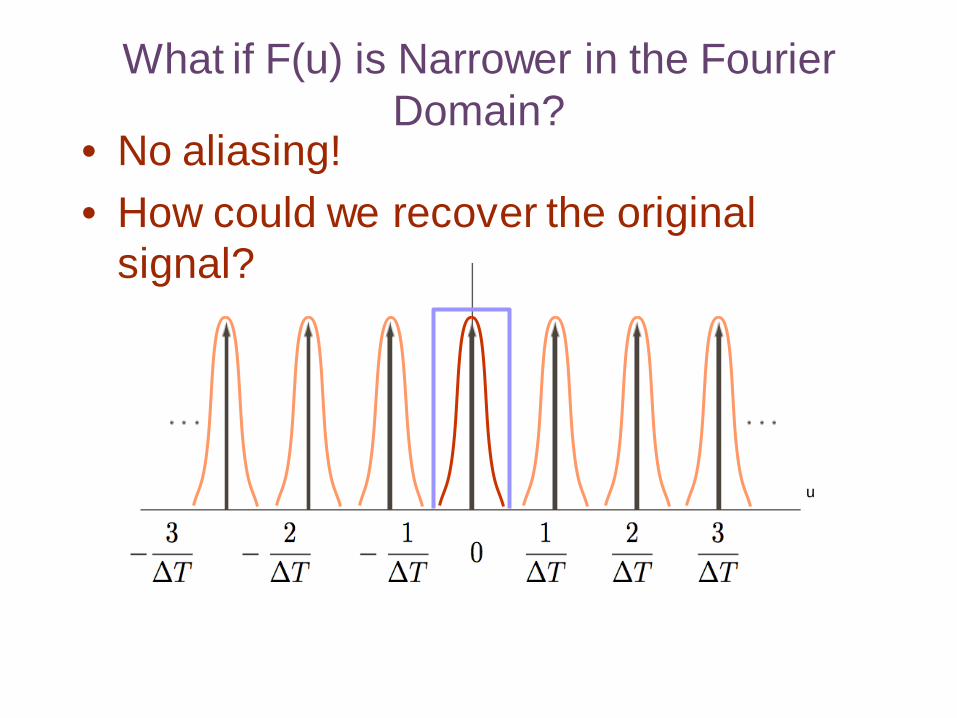
What if F(u) is Narrower in the Fourier Domain?
u
• No aliasing!• How could we recover the original
signal?
What Comes Out of This Model
• Sampling criterion for complete recovery
• An understanding of the effects of sampling– Aliasing and how to avoid it
• Reconstruction of signals from discrete samples
Shannon Sampling Theorem
• Assuming a signal that is band limited:
• Given set of samples from that signal
• Samples can be used to generate the original signal– Samples and continuous signal are
equivalent
Sampling Theorem• Quantifies the amount of information in
a signal– Discrete signal contains limited frequencies– Band-limited signals contain no more
information then their discrete equivalents• Reconstruction by cutting away the
repeated signals in the Fourier domain– Convolution with sinc function in
space/time
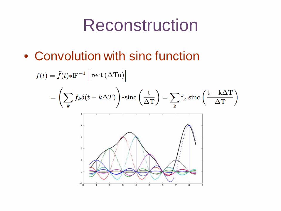
Reconstruction
• Convolution with sinc function
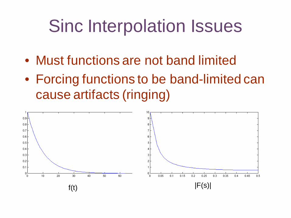
Sinc Interpolation Issues
• Must functions are not band limited• Forcing functions to be band-limited can
cause artifacts (ringing)
f(t) |F(s)|

Sinc Interpolation Issues
Ringing - Gibbs phenomenonOther issues:
Sinc is infinite - must be truncated
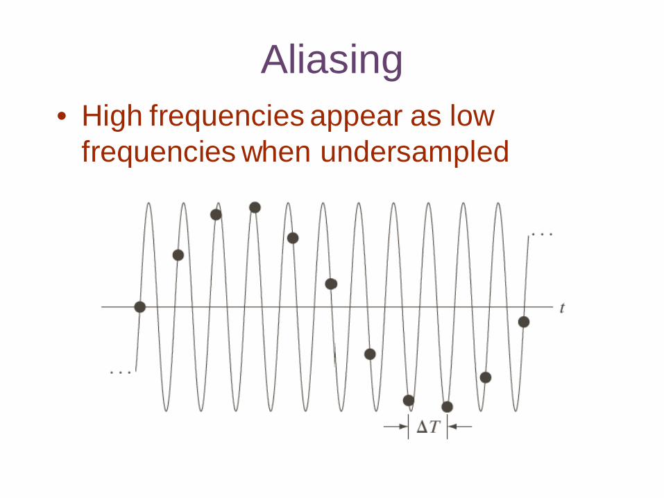
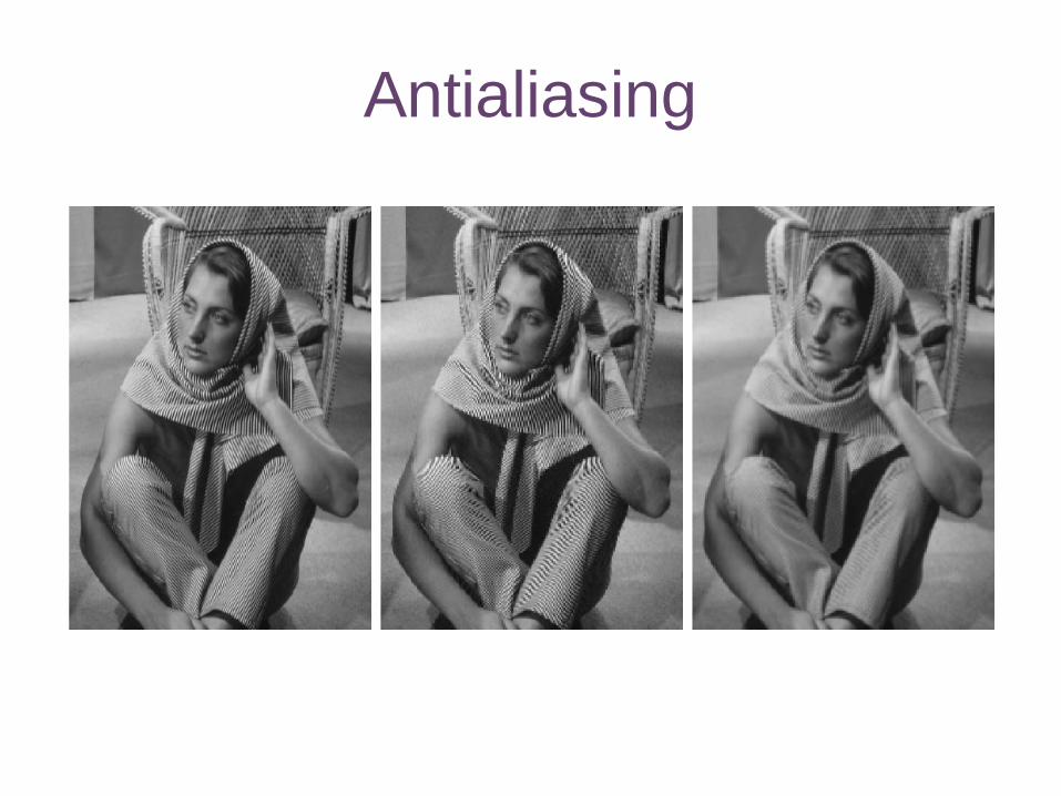
Aliasing• High frequencies appear as low
frequencies when undersampled
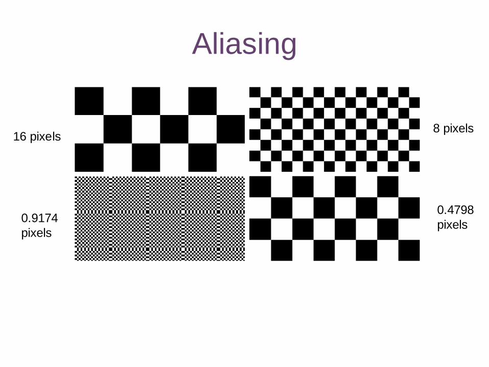
Aliasing
16 pixels8 pixels
0.9174pixels
0.4798pixels
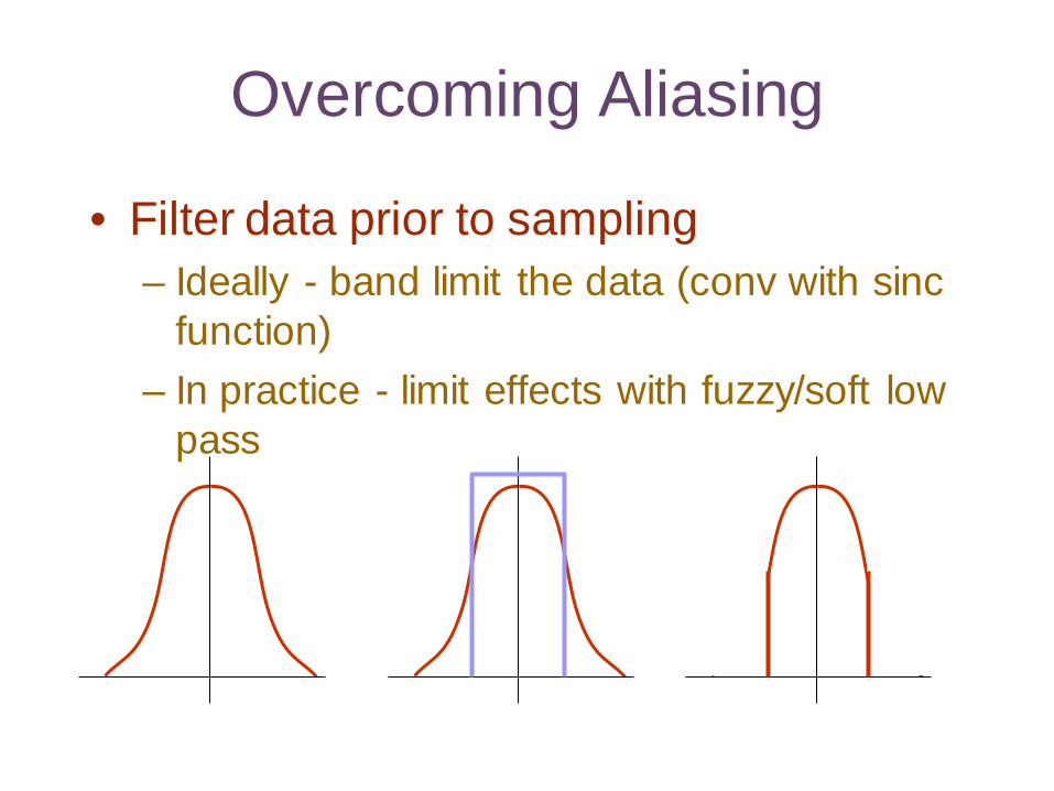
Overcoming Aliasing
• Filter data prior to sampling– Ideally - band limit the data (conv with sinc
function)– In practice - limit effects with fuzzy/soft low
pass
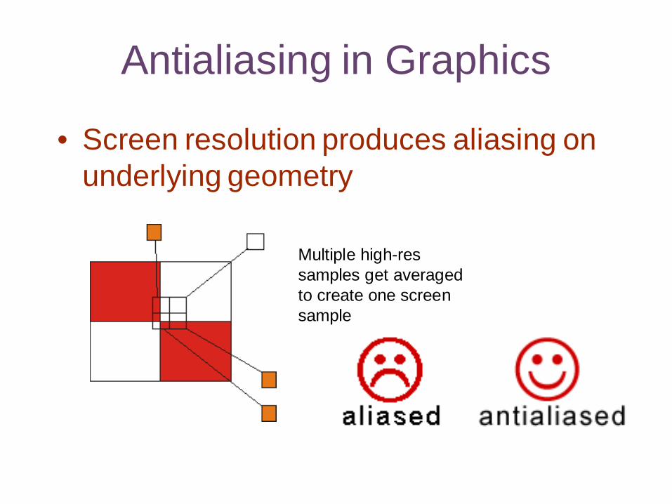
Antialiasing in Graphics
• Screen resolution produces aliasing on underlying geometry
Multiple high-res samples get averaged to create one screen sample
Antialiasing
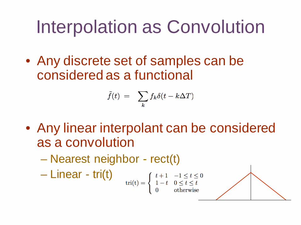
Interpolation as Convolution
• Any discrete set of samples can be considered as a functional
• Any linear interpolant can be considered as a convolution– Nearest neighbor - rect(t)– Linear - tri(t)
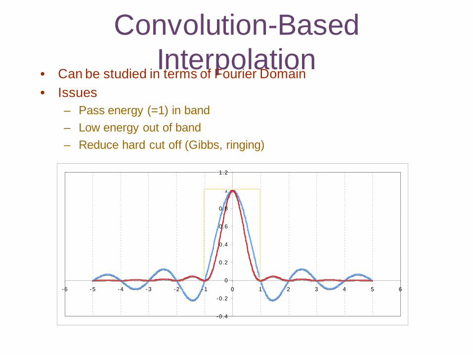
Convolution-Based Interpolation
• Can be studied in terms of Fourier Domain• Issues
– Pass energy (=1) in band– Low energy out of band– Reduce hard cut off (Gibbs, ringing)
-0.4
-0.2
0
0.2
0.4
0.6
0.8
1
1.2
-6 -5 -4 -3 -2 -1 0 1 2 3 4 5 6
Fast Fourier Transform
With slides from Richard Stern, CMU
DFT
• Ordinary DFT is O(N2)• DFT is slow for large images
• Exploit periodicity and symmetricity• Fast FT is O(N log N)• FFT can be faster than convolution
Fast Fourier Transform
• Divide and conquer algorithm• Gauss ~1805• Cooley & Tukey 1965
• For N = 2K
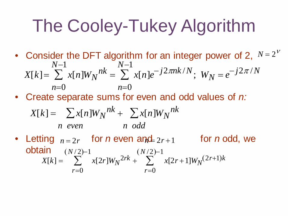
The Cooley-Tukey Algorithm• Consider the DFT algorithm for an integer power of 2,
• Create separate sums for even and odd values of n:
• Letting for n even and for n odd, we obtain
N = 2ν
X[k] =n=0
N−1∑ x[n]WN
nk =n=0
N−1∑ x[n]e− j2πnk / N ; WN = e− j2π / N
X[k] = x[n]WNnk +
n even∑ x[n]WN
nk
n odd∑
n = 2r n = 2r +1
X[k] = x[2r]WN2rk +
r=0
N / 2( )−1∑ x[2r +1]WN
2r+1( )k
r=0
N /2( )−1∑
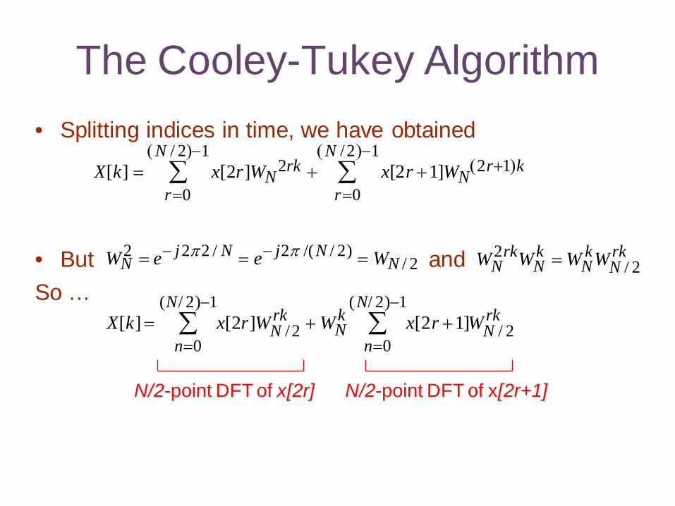
The Cooley-Tukey Algorithm• Splitting indices in time, we have obtained
• But andSo …
N/2-point DFT of x[2r] N/2-point DFT of x[2r+1]
X[k] = x[2r]WN2rk +
r=0
N / 2( )−1∑ x[2r +1]WN
2r+1( )k
r=0
N /2( )−1∑
WN2 = e− j2π2 / N = e− j2π /(N / 2) = WN / 2 WN
2rkWNk = WN
kWN / 2rk
X[k] =n=0
(N/ 2)−1∑ x[2r]WN /2
rk + WNk
n=0
(N/ 2)−1∑ x[2r +1]WN / 2
rk
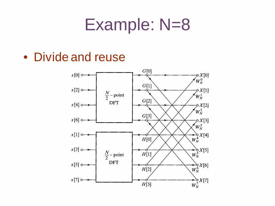
Example: N=8
• Divide and reuse
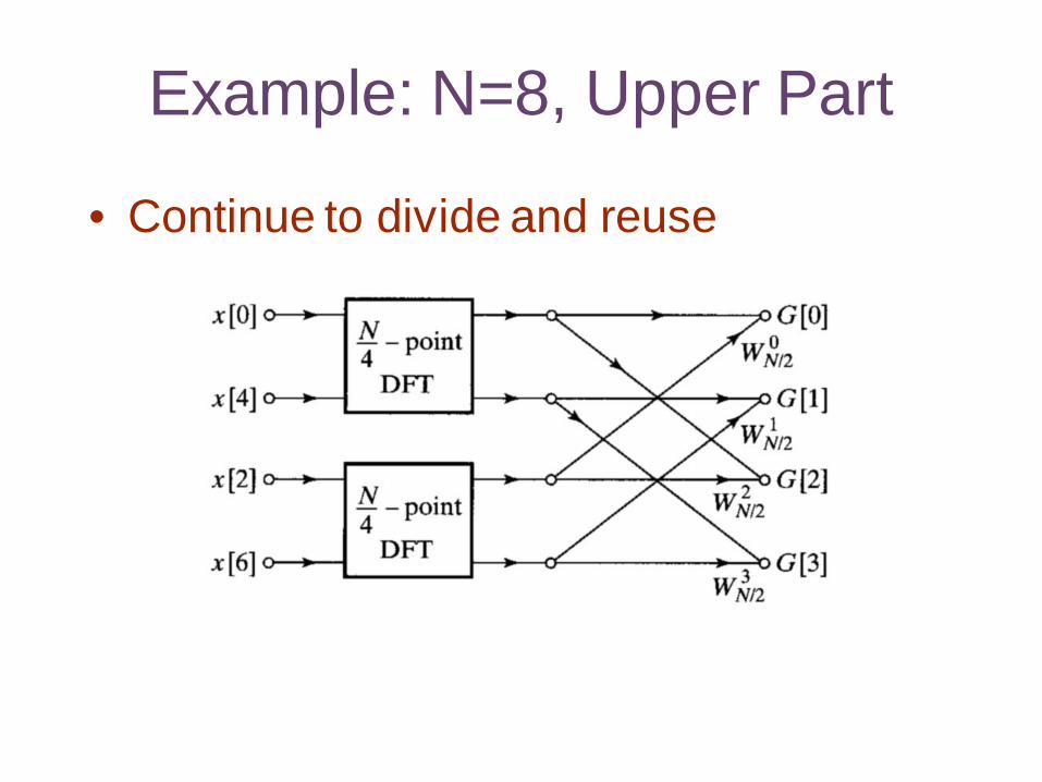
Example: N=8, Upper Part
• Continue to divide and reuse
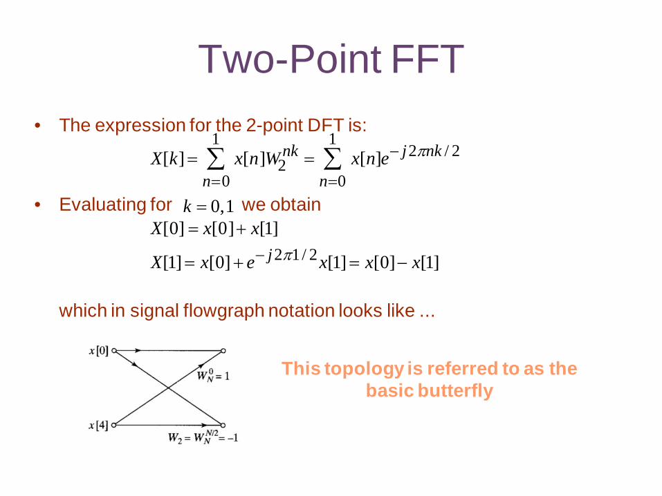
Two-Point FFT• The expression for the 2-point DFT is:
• Evaluating for we obtain
which in signal flowgraph notation looks like ...
X[k] =n=0
1∑ x[n]W2
nk =n=0
1∑ x[n]e− j2πnk / 2
k = 0,1X[0] = x[0]+ x[1]
X[1] = x[0] + e− j2π1/ 2x[1] = x[0]− x[1]
This topology is referred to as thebasic butterfly


