Fourier-transformation, phase-iteration,and least-square-fit imageprocessing for Young’s fringe pattern

Jie Gu and Fang Chen

The fast Fourier transform, phase iteration, and the least-square fit are combined into an automatedprocessing technique for the analysis of Young’s fringe patterns. A Young’s fringe pattern is firstfast-Fourier-transform filtered to get an initial phase, phase iteration is carried out to improve the phaseif necessary, and then the phase is least-square fitted to a phase plane. The magnitude and thedirection of the displacement associated with the Young’s pattern are determined from the phase plane.Key words: Young’s pattern, fast Fourier transform, phase iteration, least-square fit. r 1996

Optical Society of America

1. Introduction

In speckle photography1 two exposures are recordedon a specklegram before and after the object isdeformed. The specklegram is probed pointwise bya narrow laser beam, and Young’s fringes are dis-played in the diffraction field behind the speckle-gram, as shown in Fig. 1. The displacement vectoris determined by the spacing and the direction of theYoung’s fringe pattern. Themagnitude of a displace-ment vector d is

d 5lL

MD, 112

where l is the wavelength of the laser light,M is themagnification factor of the recording system, L is thedistance from the specklegram to the receivingscreen, and D is the spacing of the fringe pattern.The direction of a displacement vector is perpendicu-lar to the Young’s fringe lines. Although Young’spattern analysis is one of the most accurate methodsin modern optical metrology, the manual processingis rather slow, and automated image processing ofYoung’s patterns is highly desirable. Several auto-matic systems and algorithms, such as one-dimen-sional 11-D2 integration, 1-D autocorrelation, 1-D and

The authors are with the Department of Mechanical Engineer-ing, Oakland University, Rochester, Michigan 48309.Received 15December 1994; resubmittedmanuscript received 5

September 1995; accepted 5 September 1995.0003-6935@96@020232-08$06.00@0r 1996 Optical Society of America

232 APPLIED OPTICS @ Vol. 35, No. 2 @ 10 January 1996

two-dimensional 12-D2 Fourier transformation, 2-DWalsh transformation, andmaximum-likelihood tech-niques, have been proposed and evaluated in therecent literature.2–8In this paper we treat Young’s fringe analysis by a

whole-field processing method. A 2-D fast-Fourier-transform 1FFT2 filtering of a Young’s pattern pro-duces data for an initial phase calculation, thenphase iteration is used to improve the phase whennecessary. After this, a least-square regression isperformed to fit the phase to a plane. The displace-ment vector is determined precisely from this phaseplane.

2. Programming Algorithm

Figure 2 shows the flow chart of the algorithm.

A. Fourier Filtering

The light intensity of a Young’s pattern can bewritten as9

I1x, y2 5 I01x, y2 31 1 g cos f1x, y24, 122

where I01x, y2 is an autocorrelation of the pupil func-tion of the lens used to record the specklegram, g is acontrast parameter, and f1x, y2 is the phase functionof the fringe pattern. The autocorrelation functionI01x, y2 contains within it a speckle pattern related tothe Fourier transform of the probe area. Becausethe diameter of probe beam must be larger than thedisplacement in the specklegram, the halo specklesmust be finer than the halo fringes. As the Young’sfringes are supposed to be equally spaced straight

lines, the phase must be a plane:

f1x, y2 5 ax 1 by, 132

where a and b are constants. A Fourier transformof Eq. 122 gives the spectrum:

S1 fx, fy2 5 ee I1x, y2exp32j2p1xfx 1 yfy24dxdy, 142

where fx and fy are frequency coordinates in thespectrum domain. Using the Euler formula, wehave

S1 fx, fy2 5 F 5I01x, y26 1 F 5g2 I01x, y2exp3 jf1x, y2461 F 5g2 I01x, y2exp32jf1x, y246

5 F 5I01x, y26 11

2F 5gI01x, y26

p d1fx 2a

2p, fy 2

b

2p211

2F 5gI01x, y26 p d1fx 1

a

2p, fy 1

b

2p2 , 152

where F indicates a Fourier transformation and pdenotes a convolution. In a Young’s pattern, f1x, y2provides a dominant frequency. As is described inSection 5, the spectrum consists of three bright spotssurrounded by noise. The first term in Eq. 152includes an autocorrelation, which is the center spot,and a broad speckle spectrum. The second and thethird terms in Eq. 152 contain two cross-correlationpeaks and the accompanying speckle spectra. Thespectrum is filtered so that only one cross-correlationpeak is passed. A simple window, usually square inshape, covers the peak, and is approximately cen-tered on the spot. Only the spectrum inside thewindow is used, and, ideally, we select the secondterm in Eq. 152 and do an inverse Fourier transform toobtain the information:

IfP 5gI01x, y2

2exp3 jf1x, y24. 162

Fig. 1. Schematic of pointwise filtering of a Young’s pattern.

Equation 162 gives two parts, real and imaginary, andthe phase is then derived by

arctanIm1IfP2

Re1IfP25 arctan

gI01x, y2sin f1x, y2

gI01x, y2cos f1x, y25 f1x, y2.

172

In practice, additional information is generally pres-ent in the filter window and degrades the functionf1x, y2. As an illustration, we show the situation inthe 1-D case in Fig. 3. The speckle spectrum in thebottom drawing introduces noise that covers a smallrange around the pure information frequency. By

Fig. 2. Algorithm flow chart.

Fig. 3. Schematic of filtering in one dimension.

10 January 1996 @ Vol. 35, No. 2 @ APPLIED OPTICS 233

doing the same calculation in Eq. 172, we obtain aninitial phase with noise:

f01x, y2 5 arctanIm1If2

Re1If2

5 arctangI01x, y2sin f1x, y2 1 Im5E3I01x, y246

gI01x, y2cos f1x, y2 1 Re5E3I01x, y246,

182

whereE3I01x, y24 represents the inverse Fourier trans-form of the remaining noise spectrum. Fourierfiltering removes some noise, but f0 includes bothinformation and the remaining noise. The Fouriertransform in the processing program is achieved byFFT. The noise problem is treated in the followingsteps.

B. Iteration

Four phase-shifted patterns are reconstructed fromthe phase 1initial phase or improved phase2 by

Ii 5 1 1 cos k3f1n212 1p

21i 2 124 i 5 1, 2, 3, 4, 192

where n is the iteration index and k is a multiplica-tion factor. If k 5 1, for example, the fringe inten-sity of the reconstructed pattern is the same as thatof the original Young’s pattern. If k 5 2, the fringenumber is doubled. These four patterns are thensmoothed by convolutions:

Ii81x, y2 5 Ii1x, y2 p circ1x, y2, 1102

where circ1x, y2 is the smoothing window that isusually disk shaped. The smoothed patterns areput into the following equation to calculate theimproved phase:

fn1x, y2 5 arctanI48 2 I28

I18 2 I38. 1112

The above three steps can be performed severaltimes.

C. Least-Square Fit

If the major part of a phase is a linear function of thecoordinate, the iterated phase converges to thislinear function,10 and Young’s fringe patterns fallinto this category. Nevertheless, more iterationsrequire more computing time, and relative improve-ment decreases with iteration number. In the caseof analyzing Young’s pattern, one or two iterationsyield a fairly good linear function with only localfluctuations. A least-square fit is used in the nextstep to suppress the local fluctuations.For Young’s pattern analysis the useful informa-

tion consists of the two parameters that define thelinear function f1x, y2 in Eq. 132. The real phaseafter i iterations is fi. To fit the experimental data

234 APPLIED OPTICS @ Vol. 35, No. 2 @ 10 January 1996

to a linear function, we define

E 5 o 1fi 2 f22 5 o 1fi 2 axi 2 byi22, 1122

where the summation covers the area of interest 1seeFig. 92 and is done from pixel to pixel. Let

≠E

≠a5 0,

≠E

≠b5 0. 1132

We get

ao xi2 1 bo xiyi 5 o xifi,

ao xiyi 1 bo yi2 5 o yifi, 1142

and we obtain a and b by solving linear equation set1142.

3. Displacement

The gradient of the phase plane is

=f 5 1i ≠

≠x1 j

≠

≠y2f5 ai 1 bj. 1152

The maximum directional derivative of the phase is

D 5 1a2 1 b221@2. 1162

On the other hand, one fringe spacing corresponds toa 2p phase. So

D 52p

D. 1172

From Eqs. 1162 and 1172we get the fringe spacing:

D 52p

1a2 1 b221@2. 1182

The displacement is calculated by Eq. 112. Thedirection of the displacement is

n 5 61nxi 1 ny j2, 1192

where

nx 5a

1a2 1 b221@2,

ny 5b

1a2 1 b221@2, 1202

and the 6 indicates the 180° ambiguity of thespeckle displacement.

4. Experiment

The schematic of the setup is shown in Fig. 1, inwhich a specklegram is probed by a laser beam of 1mm diameter. The distance from the specklegramto the receiving screen is 50 cm. This produces aYoung’s pattern with a halo diameter of ,10.5 cm

that illuminates a receiving screen that is a piece ofground glass. The central bright spot in the halo isblocked by a stop. The fringe pattern is captured bya TV camera with a frame resolution of 512 3 512pixels. The magnification of the TV camera is ad-justed by a zooming mechanism to be 40 pixels@cm.In other words, 1 pixel covers 0.25 mm on thereceiving screen. The size of a typical secondaryspeckle is 1.2lL@diameter 5 0.4 mm, where l 5632.8 nm is the wavelength of the laser. The sam-pling process smooths the speckles in the Young’spattern to a certain extent. The sampled pattern isprocessed by a PC with a VS-100 image board.A program is designed to execute the algorithm.

We do the following: Start the program and load aYoung’s pattern, as is shown in Fig. 4. Do a forwardFFT to the pattern to get the spectrum shown inFig. 5. Move a selecting box and let it cover theuseful spectrum. Do a backward FFT, and thencalculate the initial phase shown in Fig. 6. There

Fig. 4. Original Young’s fringe pattern.

Fig. 5. Fourier spectrum.

are some major failures in Fig. 6. The phase-iteration algorithm is conducted to remove them.Do fringe reconstruction from the phase obtained.Choosing a multiplication factor of 1, we reconstructfour phase-shifted patterns. One of them, I1, isshown in Fig. 7. Then do smoothing by a disk-shaped window to all four patterns. Refer to Ref. 10for a suggestion on selecting the window size.Figure 8 is the smoothed pattern from Fig. 7. Thenext step is to perform phase calculation again fromthese new patterns and to get the phase shown inFig. 9. This phase is much better than the oneshown in Fig. 6 and does not need anymore iteration.Figure 10 is a three-dimensional view of this phasedistribution. It is almost a plane except for someminor local fluctuation. The irregularities in thefour corners in Fig. 10 are out of theYoung’s pattern’sarea. This phase is least-square fitted, and theresult is shown in Fig. 11. Figure 12 is its three-dimensional view. This fitted phase is, of course, astrict plane. The displacement vector is obtained

Fig. 6. Initial phase distribution.

Fig. 7. Fringe pattern I1 reconstructed from the wrapped phase.

10 January 1996 @ Vol. 35, No. 2 @ APPLIED OPTICS 235

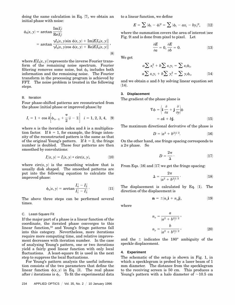
from this strict plane. If we do a fringe reconstruc-tion now from the phase in Fig. 11, we expect an idealYoung’s pattern without noise and halo effect. Thisis indeed the case 1see Fig. 132. Figures 14 and 15show two more examples. The error in our experi-ment is within 0.5%.

5. Analysis of the Young’s Pattern Spectrum

A. Spectrum of a Young’s Pattern

For simplicity we assume that the speckle displace-ment within the probing area is a constant. Sup-pose speckle irradiance patterns I11u2 and I21u2 arerecorded as a double-exposure specklegram at theplane u in Fig. 16. Pointwise filtering is usuallyperformed by transmission of a narrow collimatedlaser beam through specific points on the speckle-gram and observation of its diffraction halo at acertain distance away. Without loss of generality,we use the schematic shown in Fig. 16 for the

Fig. 8. Smoothed pattern from Fig. 7.

Fig. 9. Phase calculated from smoothed patterns and the areafor least-square fitting.

236 APPLIED OPTICS @ Vol. 35, No. 2 @ 10 January 1996

convenience of theoretical discussion. Assumingthe film that records the specklegram respondslinearly with respect to exposure, the field transmit-ted through the illumination region is

t1u2 5 s1u25a 1 b3I11u21 I21u246, 1212

where a and b are constants and the probing-beamamplitude function s1u2 is

s1u2 5 5Gaussian within probing area a

0 elsewhere. 1222

An irradiance can be decomposed into

I1u2 5 Iave 1 i1u2, 1232

where Iave is the average and i1u2 is the variablecomponent. We define the constant C as

C 5 a 1 b1I1ave 1 I2ave2, 1242

Fig. 10. Three-dimensional view of the phase distribution inFig. 9.

Fig. 11. Least-square-fitted phase.

and Eq. 1212 becomes

t1u2 5 s1u25C 1 b3i11u2 1 i21u246. 1252

The field in Young’s pattern plane is the Fouriertransform of Eq. 1252:

T1x2 5 C F 5s1u26 1 b F 5s1u26 p F 5i11u2 1 i21u26, 1262

where T1x2 5 F 5t1u26. The corresponding light-in-tensity distribution is

0T1x2 025 0CF 5s1u26 1 bF 5s1u26 p F 5i11u2 1 i21u26 02

5 0CF 5s1u26 02

1 Cb F 5s1u263 F 5s1u26 p F 5i11u2 1 i21u264*

1 CbF 5s1u26 F 5s1u26 p F 5i11u2 1 i21u26

1 0bF 5s1u26 p F 5i11u2 1 i21u26 02. 1272

Fig. 12. Three-dimensional view of the phase distribution inFig. 11.

Fig. 13. Reconstructed perfect Young’s fringe pattern.

F 5s1u26 is a common factor to the first three terms ofEq. 1272, and, because it is the transform of theprobe-beam profile, it is very much like a deltafunction. It has a large value at the origin of theYoung’s pattern plane and falls off quickly to zerobeyond the distance of a typical speckle radius,which in our experiment is 0.2 mm. Therefore thefirst three terms all contribute only to the centralbright spot of the halo and are typically blocked offbefore the halo is recorded and transformed. Drop-ping the first three terms, we have

0T1x2 02 5 b2 0 F 5s1u26 p F 5i11u2 1 i21u26 02. 1282

In performing a Fourier transform of Eq. 1282, wemay make use of the relationship

F 5 F 5s1u266 51

2ps12u2, 1292

1a2

1b2

Fig. 14. Additional example 1: 1a2Young’s pattern and 1b2 recon-structed pattern.

10 January 1996 @ Vol. 35, No. 2 @ APPLIED OPTICS 237

and this makes it possible to express the Fouriertransform of Eq. 1282 as

S1u2 5 1 b

2p22

5s12u23i112u2 1 i212u246

^ 5s12u23i112u2 1 i212u246, 1302

1a2

1b2

Fig. 15. Additional example 2: 1a2Young’s pattern and 1b2 recon-structed pattern.

Fig. 16. Young’s pattern formation.

238 APPLIED OPTICS @ Vol. 35, No. 2 @ 10 January 1996

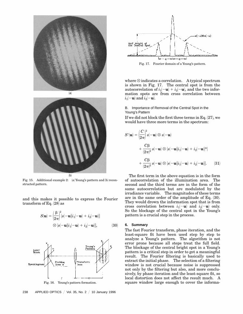
where^ indicates a correlation. A typical spectrumis shown in Fig. 17. The central spot is from theautocorrelation of i112u2 1 i212u2, and the two infor-mation spots are from cross correlation betweeni112u2 and i212u2.

B. Importance of Removal of the Central Spot in theYoung’s Pattern

If we did not block the first three terms in Eq. 1272, wewould have three more terms in the spectrum:

S81u2 5 1 C2p22

s12u2 ^ s12u2

1Cb

12p22s12u2 ^ 5s12u23i112u2 1 i212u24*6

1Cb

12p22s12u2 ^ 5s12u23i112u2 1 i212u246. 1312

The first term in the above equation is in the formof autocorrelation of the illumination area. Thesecond and the third terms are in the form of thesame autocorrelation but are modulated by theirradiance variable. Themagnitudes of these termsare in the same order of the amplitude of Eq. 1302.They would drown the information spot that is fromcross correlation between i112u2 and i212u2 only.So the blockage of the central spot in the Young’spattern is a crucial step in the process.

6. Summary

The fast Fourier transform, phase iteration, and theleast-square fit have been used step by step toanalyze a Young’s pattern. The algorithm is noterror prone because all steps treat the full field.The blockage of the central bright spot in a Young’spattern is a critical step in order to get a meaningfulresult. The Fourier filtering is basically used toextract the initial phase. The selection of a filteringwindow is not crucial because noise is suppressednot only by the filtering but also, and more conclu-sively, by phase iteration and the least-square fit, solocal distortion does not affect the result much. Asquare window large enough to cover the informa-

Fig. 17. Fourier domain of a Young’s pattern.

tion spot but centered at the information spot does adecent job, and one or two phase iterations areenough for the processing. The least-square regres-sion fits the phase into a plane that supplies theinformation of the displacement vector. The haloeffect is eliminated by use of Eq. 172 to extract theinitial phase. The experiment result is presented toconfirm the theory and the algorithm. The process-ing is automated by a personal computer with animage board.

The authors are grateful to the topical editor forhis constructive criticism and help in clarifyingSection 5.

References1. A. E. Ennos, ‘‘Speckle interferometry,’’ in Laser Speckle and

Related Phenomena, J. C. Dainty, ed. 1Springer-Verlag, Ber-lin, 19752, pp. 203–253.

2. R. Meynart, ‘‘Instantaneous velocity field measurements in

unsteady gas flow by speckle velocimetry,’’ Appl. Opt. 22,535–540 119832.

3. D. W. Robinson, ‘‘Automatic fringe analysis with a computerimage-processing system,’’Appl. Opt. 22, 2169–2176 119832.

4. J. M. Huntley, ‘‘An image processing system for the analysis ofspeckle photographs,’’ J. Phys. E. 19, 43–48 119862.

5. J. M. Huntley, ‘‘Speckle photography fringe analysis by theWalsh transform,’’Appl. Opt. 25, 382–386 119862.

6. J. M. Huntley, ‘‘Speckle photography fringe analysis: assess-ment of current algorithms,’’Appl. Opt. 28, 4316–4322 119892.

7. D. J. Chen and F. P. Chiang, ‘‘Digital processing of Young’sfringes in speckle photography,’’ Opt. Eng. 29, 1413–1420119902.

8. J. M. Huntley, ‘‘Maximum-likelihood analysis of speckle pho-tography fringe patterns,’’Appl. Opt. 31, 4834–4838 119922.

9. D. W. Li, J. B. Chen, and F. P. Chang, ‘‘Statistical analysis ofone-beam subjective laser-speckle interferometry,’’ J. Opt.Soc. Am.A 2, 657–666 119852.

10. J. Gu, Y. Y. Hung, and F. Chen, ‘‘Iteration algorithm forcomputer aided speckle interferometry,’’ Appl. Opt. 33, 5308–5317 119942.

10 January 1996 @ Vol. 35, No. 2 @ APPLIED OPTICS 239