Senior Math Seminar, Fall 2014

Matt Johnson

AbstractFourier Analysis is a powerful tool in image processing, and can be used to extract

geometric and positional information from an image. By transforming an image from the spatial domain to the frequency domain, it is possible to manipulate the structure of said

image in unexpected ways. This paper will touch on the derivation and simplification of this computationally heavy task, as well as present a few examples for the understanding

of the subject matter.

I. Introduction to Image Processing

The world we live in is full of visual beauty. This beauty is manifested with a vast

amount of shapes, colors, textures, and motions. Even though our eyes can sense and perceive

most of the world’s beauty, we may want to see it at our leisure, or simply when we can’t be in

the right place at the right time. Whatever the case may be, we look at images that have been

acquired through the use of machines every single day. It becomes somewhat of a great

challenge to give the perception capabilities of the human eye to a machine in order to interpret

the visual information that is present in our sensory world. Image processing is defined as the

acquisition, analysis, and manipulation of a digitized image, especially in order to improve its

quality. In this paper, I will go over a few real world applications of image processing, some

basic image processing concepts and methods with a bigger focus on Fourier Analysis, how

Fourier Analysis came to be a part of our world today, some of the mathematical procedures and

variations, and finally some examples of Fourier Analysis being used.

I feel that most people’s minds don’t learn something properly if they are just told what

something is and how to perform it. The one key element that is indubitably necessary is being

taught the purpose of what they’re learning: how to use it in the real world. Because of this

notion, I will put forth an incomplete list of examples in which image processing is used in order

to give you – the reader – some motivation behind learning it. Among these examples are:

special effects in videos, facial recognition software, vision-guided robotics, vision-based

diagnosis such as X-rays, astronomical image enhancement, missile guidance, surveillance, and

traffic monitoring. I won’t go into full detail of any of these areas, but in each example, image

processing is taking place. This means that a picture is taken, being analyzed, and manipulated in

some way, shape, or form. So it is evident that image processing goes beyond putting a filter on

an Instagram photo; there are actually very useful applications of it. Next I will explain the basic

principles of image processing.

a. Image Acquisition

Image acquisition is the first step to the entirety of image processing. In the big picture, it

can be described as simply obtaining an image to be worked with. This step requires the use of

some sort of sensor in optical or thermal wavelengths. The result of image acquisition is the

mapping of the three-dimensional visual world onto a two-dimensional plane surface. This can

also be called rendering: a three-dimensional scene is rendered into a two-dimensional image.

Now, it just so happens that, more often than not, the image that has been acquired is not of the

ideal quality. By this, it is meant that the picture is not immediately in the right condition to be

viewed by the person (or thing) that is meant to view it. Some examples include noise and blur.

Some causes of these effects in images include motion between the object and the camera and

atmospheric conditions.

b. Image Analysis

After we have acquired an image, we can move on to the next step: image analysis.

Image analysis can be defined as the extraction of meaningful information from images. When

enhancing an image this step can be thought of as extracting information that is unneeded, and

then removing it from the image altogether. This can be done to find out what needs to be

changed in a picture before it’s ready to be viewed. A further look at this part in the process

reveals a sub process called segmentation. In this portion, the entire original image is subdivided

into separate homogeneous regions. For example, an image consisting of a shore might have a

region with water and a region with land. These two regions may then be further subdivided, and

so on. Other things to extract from each region, after segmentation, are features such as texture,

shape, and color. The idea is to classify each region into a sort of hierarchy of meaningful

classifications. I could go on all day about this process, but the focus here is to get the basic

principles across.

c. Image Manipulation

The last step, after acquisition and analysis, is manipulation. So now we have an image

and we know what should be changed about it. Naturally, the next thing to do is to commit those

changes. Keep in mind that this doesn’t always involve a human consciously making these

changes with software such as Adobe Photoshop, even though Photoshop comes equipped with

mostly all manipulation features. Much of the time, the process consists of taking each individual

pixel (picture element) and putting it through a function, such is the case with Fourier Analysis.

We will dive deeper into that territory later, however.

II. History

Now that I have introduced the basic ideas and principles of image processing as well as

some motivation behind learning it, we can start getting into Fourier Series and the Fourier

Transform, and how they apply to image processing.

The Fourier Series is named after Jean-Baptiste Joseph Fourier. His purpose for

proposing this idea was to solve the heat equation in a metal plate. At the time, there was no

solution to the heat equation in a general sense; only in simple cases. These simple cases only

occurred if the heat source behaved like a sinusoidal wave. Given this problem, Fourier made it

his goal to model any heat source as a weighted sum of sine and cosine waves. This sum came to

be known as the Fourier Series. Although the original motive for coming up with this series was

to solve the heat equation, it became apparent that representing any function as a sum of sine and

cosine waves was very useful and could be applied to other areas of mathematical and physical

problems. Some of these areas include quantum mechanics, econometrics, acoustics, optics,

signal processing, electrical engineering, vibration analysis, and (our topic of discussion) image

processing.

Based on the Fourier Series representation of a function, we can lengthen the represented

function’s period to allow it to approach infinity. This means that the function being represented

doesn’t even need to be periodic over some interval since the interval is the function’s entire

domain. From this method, the Fourier Transform was born. What’s neat about the Fourier

Transform is that an Inverse Fourier Transform exists. To that extent, the purpose of the Fourier

Transform in most applications is to transform a difficult problem into a problem in another

domain, solve the relatively easy problem, and then invert the Fourier Transform to come to the

solution in the original domain. This is usually the preferred route to take opposed to the

difficult, sometimes impossible, original problem.

So how does this relate to image processing? According to Fourier Theory, any signal

can be expressed as a sum of a series of sinusoids. In a two-dimensional image, these would just

be variations in brightness across the image. The original image would be the input to the

transform function. The transformed image simultaneously encodes information of each input

pixel. This information includes spatial frequency, magnitude, and phase. Based on this

information, it is possible to make modifications to the transformed image, that is, we can filter

out some undesired frequencies. After modifications have been made, we can use the Inverse

Fourier Transform to bring back the image in the spatial domain – the domain that typically

makes sense to the human eye.

III. Fourier Series Representations

a. Traditional

Now let’s start using some math. As stated earlier, Fourier came up with a way to

approximate a continuous function using weighted sums of sines and cosines. I won’t go over

many of the details, but here is what he came up with:

f ( x )=a0

2+∑n=1

∞

an ∙cos (nω0 x )+bn ∙ sin (nω0 x);n=1,2,3 ,…

Where

a0=2T0∫T 0

❑

f ( x )dx

an=2T 0

∫T 0

❑

f ( x )cos (nω0 x )dx

bn=2T 0

∫T0

❑

f ( x )sin (nω0 x)dx

If f (x) is periodic, let T 0 be the smallest T satisfying the equation f ( x+T )=f (x ) (called the

fundamental period), let f 0=1T0

(called the fundamental frequency), and let ω0=2πT0

=2 π f 0

(called the fundamental angular frequency).

Note: ∫T 0

❑

❑ denotes integrating over any continuous interval of lengthT 0.

This can all be a little confusing, so let’s go ahead and do a very simple example.

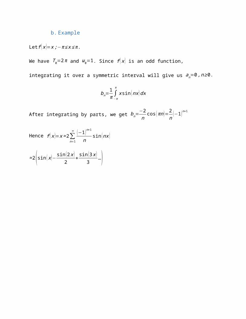
b. Example

Letf ( x )=x ;−π ≤ x≤ π.

We have T 0=2π and ω0=1. Since f ( x ) is an odd function, integrating it over a symmetric

interval will give us an=0 , n≥0.

bn=1π∫−π

π

x sin (nx )dx

After integrating by parts, we get bn=−2n

cos (πn )=2n

(−1 )n+1

Hence f ( x )=x ≈2∑n=1

∞ (−1 )n+1

nsin (nx )

≈2(sin ( x )− sin (2 x )2

+sin (3x )

3…)

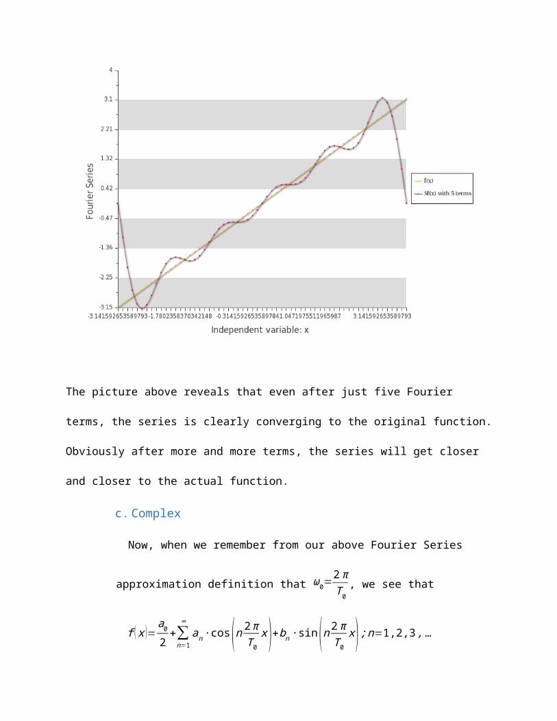
The picture above reveals that even after just five Fourier terms, the series is clearly converging

to the original function. Obviously after more and more terms, the series will get closer and

closer to the actual function.

c. Complex

Now, when we remember from our above Fourier Series approximation definition that

ω0=2πT0

, we see that f ( x )=a0

2+∑n=1

∞

an ∙cos (n 2πT0

x )+bn ∙ sin(n 2πT0

x );n=1,2,3 ,…

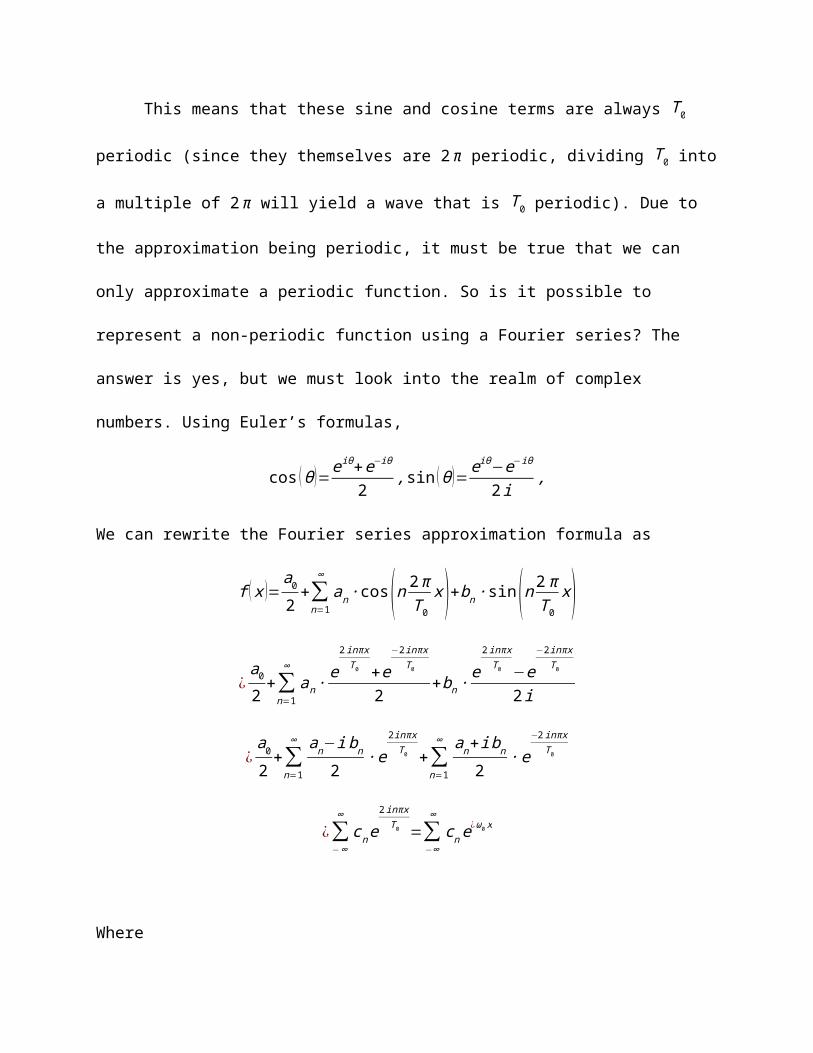
This means that these sine and cosine terms are always T 0 periodic (since they

themselves are 2π periodic, dividing T 0 into a multiple of 2π will yield a wave that is T 0

periodic). Due to the approximation being periodic, it must be true that we can only approximate

a periodic function. So is it possible to represent a non-periodic function using a Fourier series?

The answer is yes, but we must look into the realm of complex numbers. Using Euler’s formulas,

cos (θ )= eiθ+e−iθ

2, sin (θ )= e iθ−e−iθ

2i,

We can rewrite the Fourier series approximation formula as

f ( x )=a0

2+∑n=1

∞

an ∙cos (n 2πT0

x )+bn ∙ sin(n 2πT0

x )

¿a0

2+∑n=1

∞

an∙e

2 inπxT0 +e

−2inπxT0

2+bn ∙

e2 inπxT0 −e

−2 inπxT0

2i

¿a0

2+∑n=1

∞ an−i bn2

∙ e2 inπxT 0 +∑

n=1

∞ an+ ibn

2∙ e

−2 inπxT 0

¿∑−∞

∞

cn e2inπxT 0 =∑

−∞

∞

cn e¿ω0 x

Where

c0=a0

2, cn=

an− ibn

2, c−n=

an+i bn2

Using our formulas for an and bn from earlier,

cn=12¿

¿ 1T0∫T 0

❑

f ( x ) (cos (nω0 x )−isin (nω0 x )) dx

¿ 1T0∫T 0

❑

f ( x )( e¿ω0 x+e−¿ω0 x

2− ie¿ω0 x−ie−¿ω0 x

2 i )dx

¿ 1T0∫T 0

❑

f ( x )( 2e−¿ω0 x

2 )dx

cn=1T 0

∫T0

❑

f ( x ) e−¿ω0x dx; n=0 , ±1 ,±2 ,…

These coefficients are called complex Fourier coefficients. Note that the formula reduces to the

same value when using a negative n. Also note that this definition still requires that the function

be periodic since we’re still using the fundamental period T 0 .

IV. Derivation of the Continuous Fourier Transform

This is where we extend the period of the function to be infinite. At this point it will be beneficial

to redefine the variable representing our period:

T 0=2 L,where we use the interval [−L, L]

Thus we have

f ( x )=∑−∞

∞

cn einπxL

cn=1

2 L∫−L

L

f (x ) e−inπxL dx

So let us find out what happens when we allow L→∞ . We first let ω=nπL

and

Δω=ωn+1−ωn=πL. So,

f ( x )=∑−∞

∞

cn eiωx

cn=Δω2 π

∫−L

L

f ( x ) e−iωx dx

And cω=2Lcn=cn2πΔω

So now,

f ( x )=∑−∞

∞ cω2 π

Δωeiωx and cω=∫−L

L

f ( x )e−iωx dx

Now, since ω=nπL→0as L→∞, cωseems like a function of ω, which is a frequency. Let’s name

this function F (ω ) . Here we have

f ( x )= limL→∞ (Δω→0 )

∑−∞

∞ cω2 π

Δωe iωx= 12π

∫−∞

∞

F (ω) eiωx dω

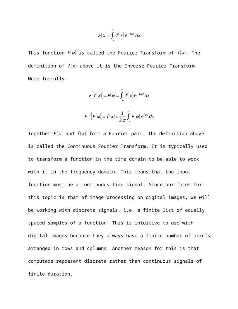
F (ω )=∫−∞

∞

f ( x ) e−iωx dx

This function F (ω ) is called the Fourier Transform of f ( x ) . The definition of f (x) above it is the

Inverse Fourier Transform. More formally:

F [ f (x ) ]=F (ω )=∫−∞

∞

f ( x )e−iωx dx

F−1 [F (ω) ]=f ( x )= 12π

∫−∞

∞

F (ω ) eiωx dω

Together F (ω) and f (x) form a Fourier pair. The definition above is called the Continuous

Fourier Transform. It is typically used to transform a function in the time domain to be able to

work with it in the frequency domain. This means that the input function must be a continuous

time signal. Since our focus for this topic is that of image processing on digital images, we will

be working with discrete signals, i.e. a finite list of equally spaced samples of a function. This is

intuitive to use with digital images because they always have a finite number of pixels arranged

in rows and columns. Another reason for this is that computers represent discrete rather than

continuous signals of finite duration.

V. Discrete Fourier Transform

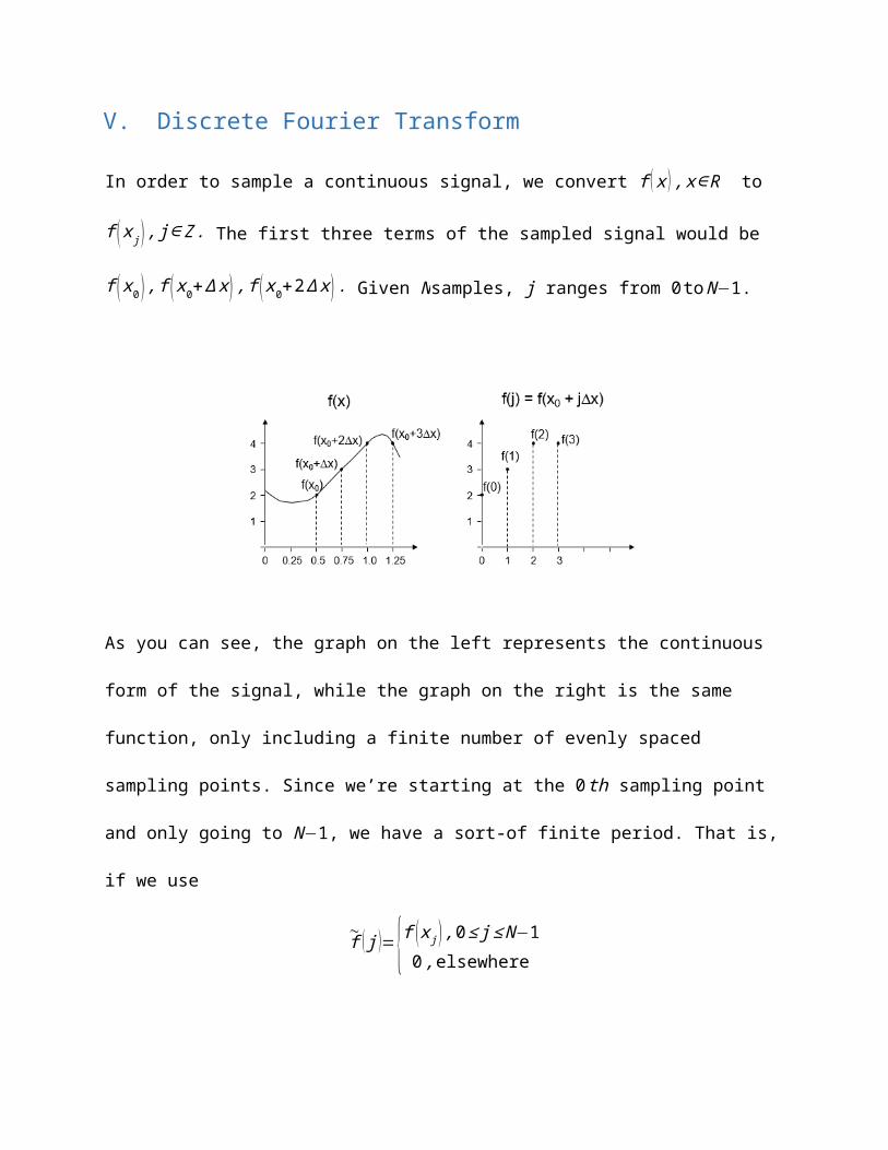
In order to sample a continuous signal, we convert f ( x ) , x∈R to f (x j ) , j∈Z . The first three

terms of the sampled signal would be f (x0 ) , f (x0+Δ x) , f (x0+2 Δ x ) . Given Nsamples, j ranges

from 0 toN−1.

As you can see, the graph on the left represents the continuous form of the signal, while the

graph on the right is the same function, only including a finite number of evenly spaced sampling

points. Since we’re starting at the 0 th sampling point and only going to N−1, we have a sort-of

finite period. That is, if we use

~f ( j )={f (x j) ,0≤ j ≤N−1

0 ,elsewhere

Then ~f ( j ) is a function of period N . This allows us to represent the function as a series again. I

won’t go over the full derivation of this next series, but it is very closely related to the

Continuous Fourier Transform, and it is known as the Discrete Fourier Transform (DFT):

F ( k )= 1√N ∑

j=0

N−1

f ( j ) ∙ e−2iπjk

N

With its inverse:

f ( j )= 1√N ∑

k=0

N−1

F (k ) ∙ e2 iπjkN

Note that the constant 1

√N is multiplied by both sums. This is because it is a normalization

constant. It doesn’t have to be used in both the forward and inverse transforms. Sometimes the

constant 1N

is used in just one of the equations, depending on the needs of the computation.

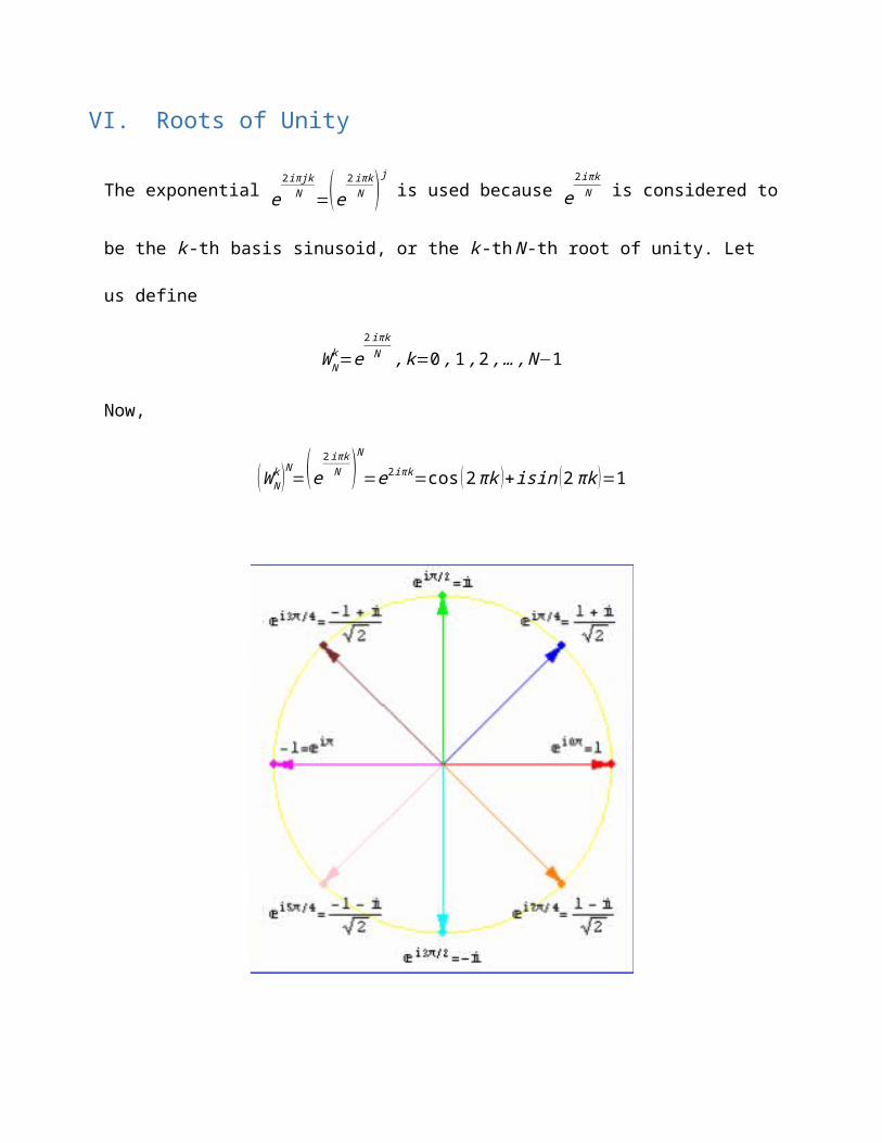
VI. Roots of Unity

The exponential e2 iπjkN =(e 2 iπk

N )j is used because e2 iπkN is considered to be the k -th basis sinusoid, or

the k -th N -th root of unity. Let us define

W Nk =e

2 iπkN , k=0 ,1,2 ,…,N−1

Now,

(W Nk )N=(e2 iπk

N )N=e2 iπk=cos (2 πk )+isin (2πk )=1

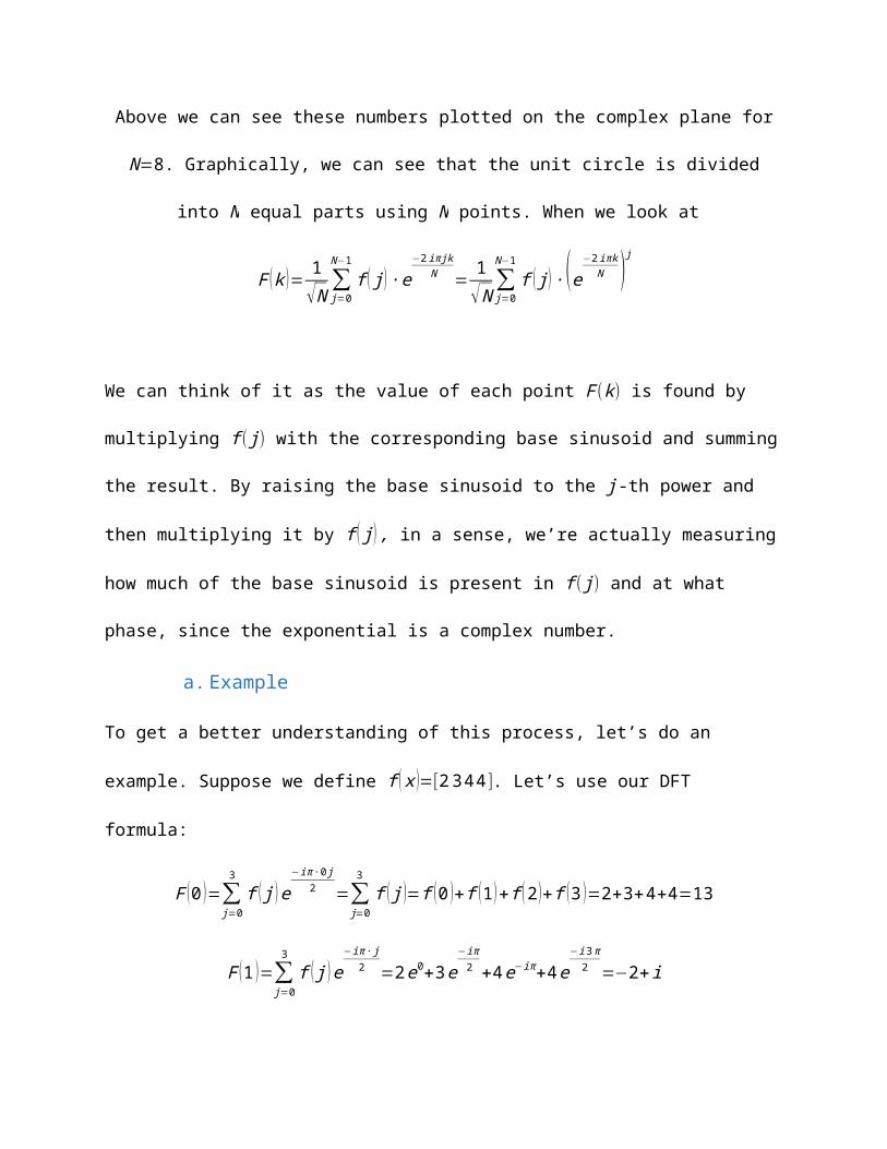
Above we can see these numbers plotted on the complex plane for N=8. Graphically, we can see

that the unit circle is divided into N equal parts using N points. When we look at

F ( k )= 1√N ∑

j=0

N−1

f ( j ) ∙ e−2iπjk

N = 1√N ∑

j=0

N−1

f ( j ) ∙ (e−2 iπkN ) j

We can think of it as the value of each point F (k ) is found by multiplying f ( j) with the

corresponding base sinusoid and summing the result. By raising the base sinusoid to the j -th

power and then multiplying it by f ( j ) , in a sense, we’re actually measuring how much of the

base sinusoid is present in f ( j) and at what phase, since the exponential is a complex number.

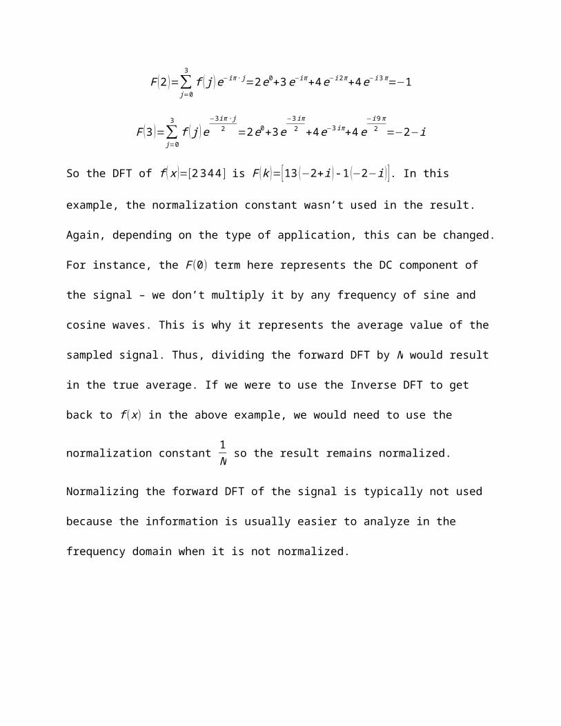
a. Example

To get a better understanding of this process, let’s do an example. Suppose we define

f ( x )=[23 44 ]. Let’s use our DFT formula:

F (0 )=∑j=0

3

f ( j ) e−iπ ∙0 j

2 =∑j=0

3

f ( j )=f (0 )+ f (1 )+ f (2 )+ f (3 )=2+3+4+4=13

F (1 )=∑j=0

3

f ( j ) e−iπ ∙ j

2 =2e0+3e−iπ

2 +4 e−iπ+4 e−i3π

2 =−2+i

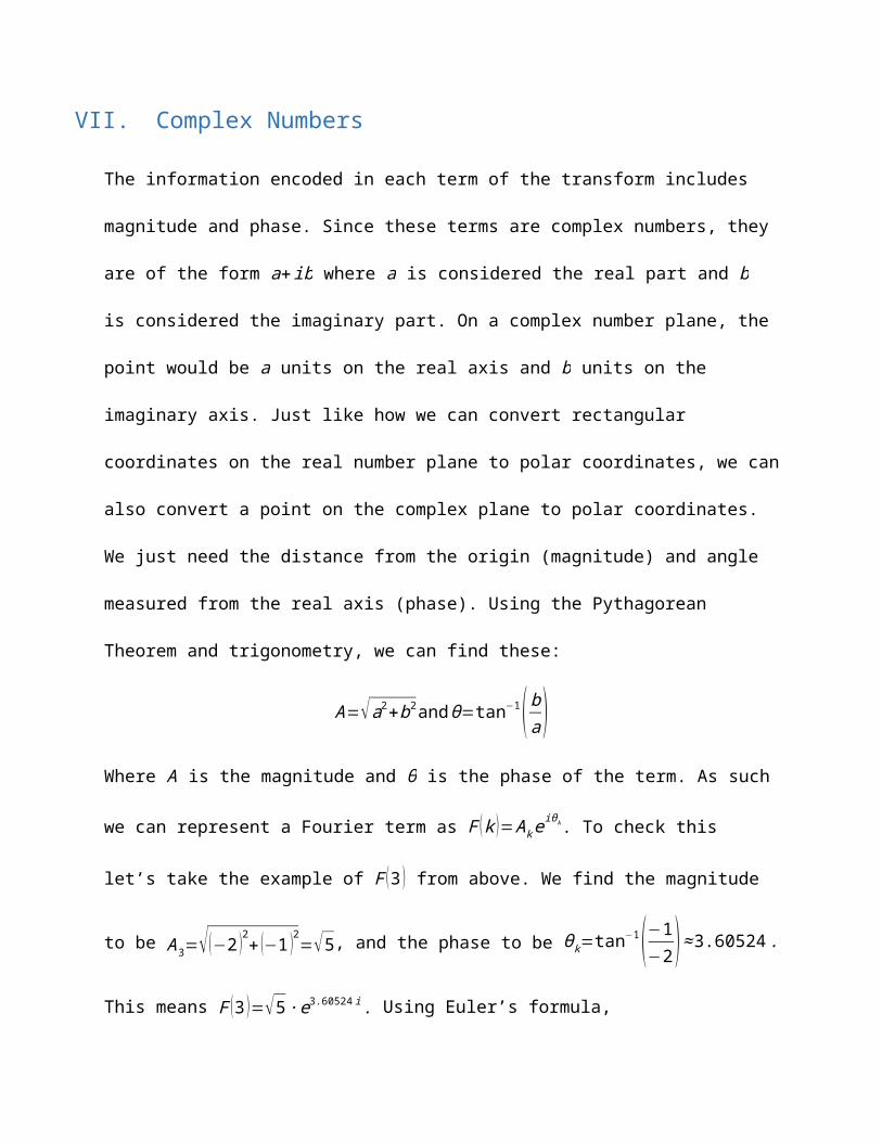
F (2 )=∑j=0

3

f ( j )e−iπ ∙ j=2e0+3e−iπ+4 e−i2π+4e−i3π=−1

F (3 )=∑j=0

3

f ( j )e−3 iπ ∙ j

2 =2e0+3e−3 iπ

2 +4 e−3 iπ+4e−i9π

2 =−2−i

So the DFT of f ( x )=[23 44 ] is F ( k )=[13 (−2+i ) -1 (−2−i ) ]. In this example, the normalization

constant wasn’t used in the result. Again, depending on the type of application, this can be

changed. For instance, the F (0) term here represents the DC component of the signal – we don’t

multiply it by any frequency of sine and cosine waves. This is why it represents the average

value of the sampled signal. Thus, dividing the forward DFT by N would result in the true

average. If we were to use the Inverse DFT to get back to f (x) in the above example, we would

need to use the normalization constant 1N

so the result remains normalized. Normalizing the

forward DFT of the signal is typically not used because the information is usually easier to

analyze in the frequency domain when it is not normalized.

VII. Complex Numbers

The information encoded in each term of the transform includes magnitude and phase. Since

these terms are complex numbers, they are of the form a+ ib where a is considered the real part

and b is considered the imaginary part. On a complex number plane, the point would be a units

on the real axis and b units on the imaginary axis. Just like how we can convert rectangular

coordinates on the real number plane to polar coordinates, we can also convert a point on the

complex plane to polar coordinates. We just need the distance from the origin (magnitude) and

angle measured from the real axis (phase). Using the Pythagorean Theorem and trigonometry,

we can find these:

A=√a2+b2 andθ=tan−1( ba )Where A is the magnitude and θ is the phase of the term. As such we can represent a Fourier

term as F ( k )=A kei θk. To check this let’s take the example of F (3 ) from above. We find the

magnitude to be A3=√(−2 )2+(−1 )2=√5, and the phase to be θk=tan−1(−1−2 )≈3.60524 . This

means F (3 )=√5∙ e3.60524 i . Using Euler’s formula,

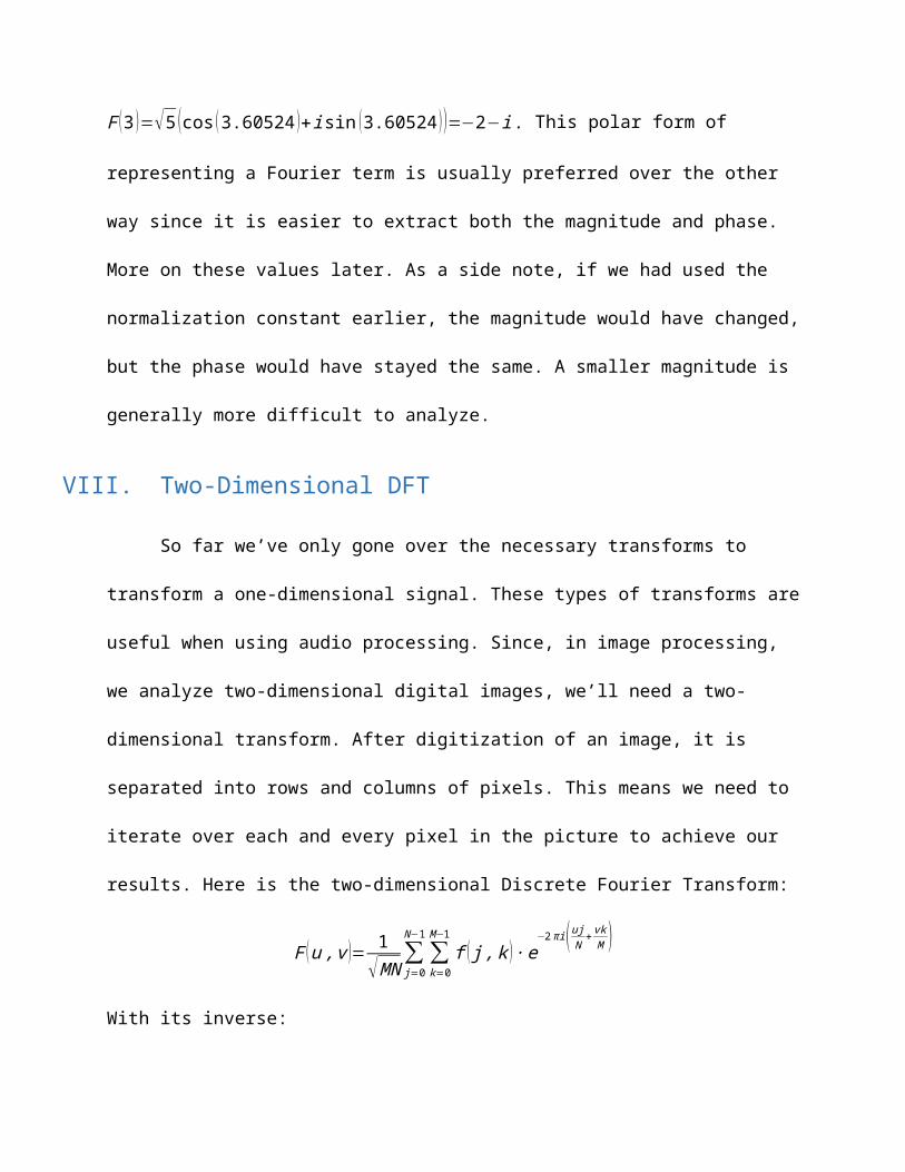
F (3 )=√5 ( cos (3.60524 )+i sin (3.60524 ))=−2−i . This polar form of representing a Fourier term

is usually preferred over the other way since it is easier to extract both the magnitude and phase.

More on these values later. As a side note, if we had used the normalization constant earlier, the

magnitude would have changed, but the phase would have stayed the same. A smaller magnitude

is generally more difficult to analyze.

VIII. Two-Dimensional DFT

So far we’ve only gone over the necessary transforms to transform a one-dimensional

signal. These types of transforms are useful when using audio processing. Since, in image

processing, we analyze two-dimensional digital images, we’ll need a two-dimensional transform.

After digitization of an image, it is separated into rows and columns of pixels. This means we

need to iterate over each and every pixel in the picture to achieve our results. Here is the two-

dimensional Discrete Fourier Transform:

F (u , v )= 1

√MN ∑j=0

N−1

∑k=0

M−1

f ( j , k ) ∙ e−2πi( ujN+ vk

M )

With its inverse:

f ( j ,k )= 1

√MN ∑u=0

N−1

∑v=0

M−1

F (u , v ) ∙ e2πi( ujN + vk

M )

Where f (x , y ) is the image in the spatial domain, and the exponential term is the basis function

corresponding to each point F (u , v ) in the frequency domain (Fourier domain). One important

thing to note here is that f (x , y ) is actually defined by the brightness of the pixel in the spatial

domain image. This could technically include different values as well (including color or depth),

but for our purposes, we’ll just assume that we’re looking at grayscale images, also called

brightness images. Typically upon image acquisition, the image is in analog form in a two-

dimensional continuous space. During image sampling (digitization), the image is converted into

digital form in a two-dimensional discrete space. After digitization occurs, each pixel is

measured for brightness. The value that is assigned to it is the average brightness of the pixel

rounded to the nearest integer. This can be seen as the amplitude of a wave at that location. There

will be a set L of gray levels that may be assigned. This number is generally a power of two. If

our set L contains 64different gray levels, a completely black pixel would be assigned a value of

0 and a completely white pixel would be assigned63. Technically speaking, a black pixel would

have a negative amplitude, but we want to represent the pixels using positive numbers. The

process of representing the amplitude of the two-dimensional signal at a given coordinate value

as an integer value with L possible gray levels is called quantization. I could write a whole

different paper on that subject alone so I’ll just leave it at that. The main point here is the fact

that the image in the spatial domain, at any given pixel coordinate, is (usually) defined by a

single, integer brightness level.

IX. Computation Speed-Up

Now, since the DFT uses a sampled function which represents the entire spatial domain image, it

does not contain every single frequency that forms an image; just a set of samples that is large

enough to fully describe it. The number of frequencies in the frequency domain corresponds to

the number of pixels in the spatial domain. This means that the frequency image will be the same

size as the spatial image. The formula above would be the DFT of an N ×M image, where N is

the number of rows and M is the number of columns. The terms in the Fourier domain represent

increasing frequencies, where F (0,0 ) is the DC component and F (N−1 ,M−1 ) represents the

highest frequency. Like mentioned previously, each DFT term is basically a measure of how

much of that frequency is present in the image. The higher the presence of that frequency in the

spatial domain image, the brighter the corresponding pixel in the Fourier domain.

There are three main categories of operations that can be applied to digital images in order to

change an input image to an output image: point, local and global operations. A point operation

is one in which the output value at a certain point depends only on that same point in the input

image. A local operation is one in which the output value at a certain point depends on the input

values in the neighborhood of that same point. A global operation is one in which the output

value at a certain point is dependent on every single value in the input image. Since the DFT

cycles through every pixel in the input image to calculate a point that represents one frequency in

the Fourier domain, it is considered a global operation. Going through the DFT one pixel at a

time is very time consuming and inefficient.

a. Separability

The two-dimensional DFT has the property of separability so that

F (u , v )=∑j=0

N−1

∑k=0

M−1

f ( j , k ) ∙ e−2πi( ujN+ vk

M )

¿∑j=0

N−1 (∑k=0

M−1

f ( j , k ) ∙ e−2πi( vkM ))e−2πi (ujN )

¿∑j=0

N−1

F ( j , v ) ∙ e−2πi( ujN )

Where

F ( j , v )=∑k=0

M−1

f ( j , k ) ∙e−2πi ( vkM )

What’s actually happening here is that we’re performing a 1D transform on each column of

spatial domain image f ( j , k ), yielding the intermediate image F ( j , v ). Then we’re performing

another 1D transform on each row of F ( j , v ), yielding the final Fourier domain image F (u , v ).

In this way, an n-dimensional transform can be computed using n one-dimensional transforms,

thus speeding up the entire process. However even with this speed up, the DFT will still have a

complexity of N2 per pixel (for a square N ×N image), which isn’t very fast. By using another

algorithm, known as the Fast Fourier Transform (FFT), this complexity can be reduced to

N log2 N per pixel. This is a much faster way especially for large images.

b. Fast Fourier Transform

The FFT works by splitting the problem up into a series of smaller problems. It utilizes the

property of symmetry in the DFT. If we have a generic transform:

F ( k )=∑n=0

N−1

f (n ) ∙ e−2πikn

N

We can see that

F (N+k )=∑n=0

N−1

f (n ) ∙ e−2πi (k +N )n

N

¿∑n=0

N−1

f (n ) ∙ e−2πin ∙ e−2πikn

N

Since e−2πin=cos (−2πn )+i sin (−2πn )=1 ∀n∈Z, we find that

F (N+k )=∑n=0

N−1

f (n ) ∙ e−2πikn

N =F (k )

This shows the periodic property of the DFT. Using this knowledge, we can say that

F ( k )=F (nN +k ) ∀n∈Z . While this doesn’t really help us in the current form since 0≤k<N , we

can utilize this fact in a smaller interval after splitting up the summation:

F ( k )=∑n=0

N−1

f (n ) ∙ e−2πikn

N

¿ ∑m=0

N2

−1

f (2m ) ∙ e−2πik ( 2m)

N +∑m=0

N2

−1

f (2m+1 ) ∙ e−2πik ( 2m+1)

N

¿ ∑m=0

N2

−1

f (2m ) ∙ e−2πikm(N /2) +e

−2πikN ∑

m=0

N2

−1

f (2m+1 ) ∙ e−2πikm(N /2)

The single DFT has been split into two terms which are very similar to a single, smaller DFT,

one on the even numbered values, and one on the odd numbered values. Just from these two

terms, we haven’t saved any computation since each term consists of N2

∗N computations for a

total of N2 . The trick comes into play when we use symmetries of each of these terms. Because

0≤k<N and 0≤m< N2

, the symmetry from above means we only need to compute half the

computations for each sub-problem. Ideally, this process would continue until there are N

signals composed of a single point (meaning N is a power of 2), but it isn’t required for the

speed up to be effective.

X. Application

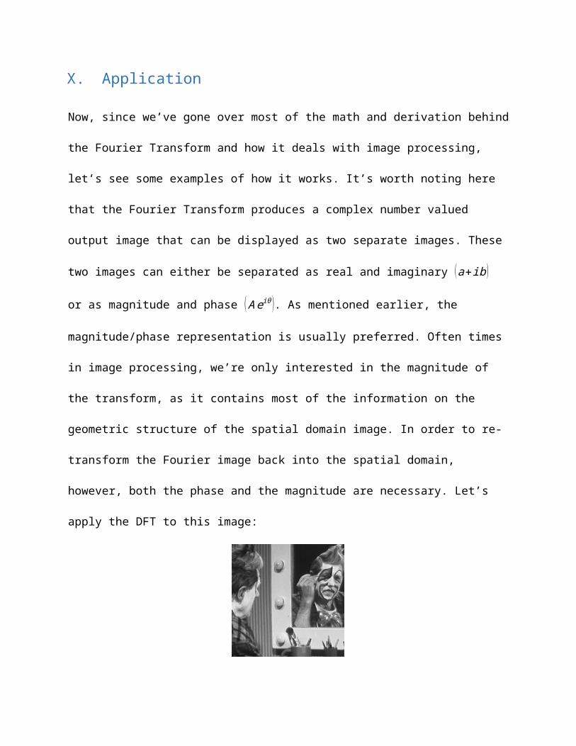
Now, since we’ve gone over most of the math and derivation behind the Fourier Transform and

how it deals with image processing, let’s see some examples of how it works. It’s worth noting

here that the Fourier Transform produces a complex number valued output image that can be

displayed as two separate images. These two images can either be separated as real and

imaginary (a+ ib) or as magnitude and phase ( Ae iθ ). As mentioned earlier, the magnitude/phase

representation is usually preferred. Often times in image processing, we’re only interested in the

magnitude of the transform, as it contains most of the information on the geometric structure of

the spatial domain image. In order to re-transform the Fourier image back into the spatial

domain, however, both the phase and the magnitude are necessary. Let’s apply the DFT to this

image:

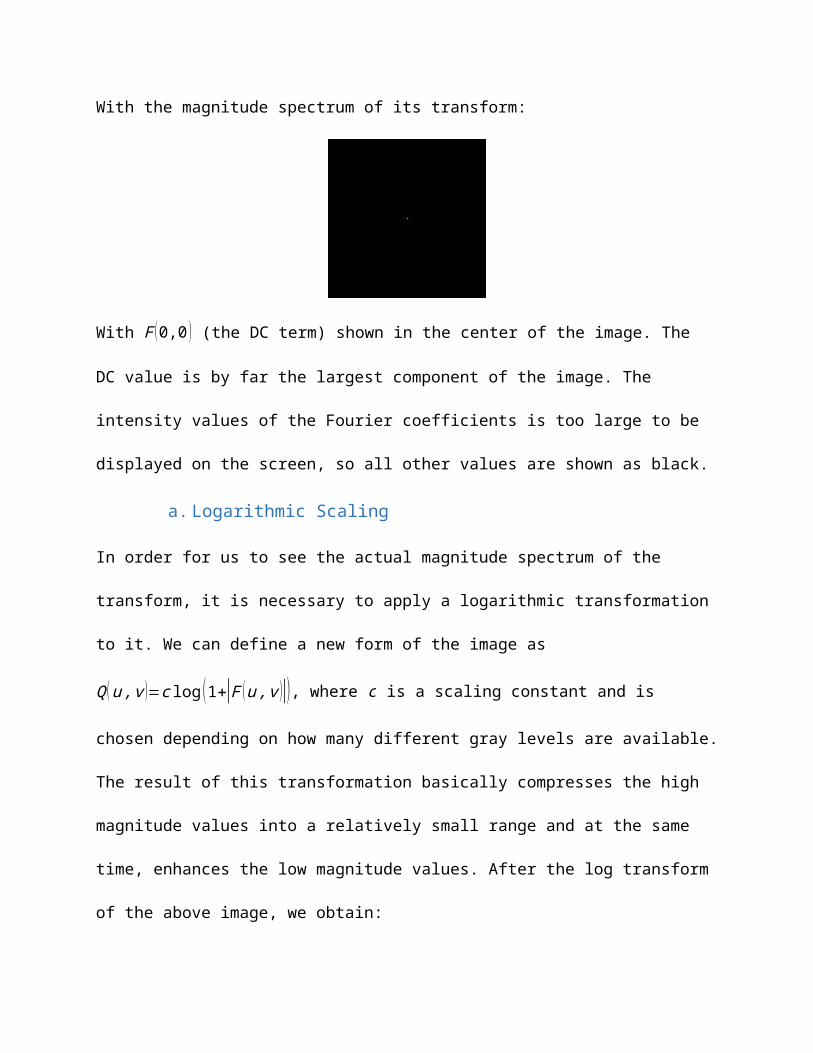
With the magnitude spectrum of its transform:

With F (0,0 ) (the DC term) shown in the center of the image. The DC value is by far the largest

component of the image. The intensity values of the Fourier coefficients is too large to be

displayed on the screen, so all other values are shown as black.

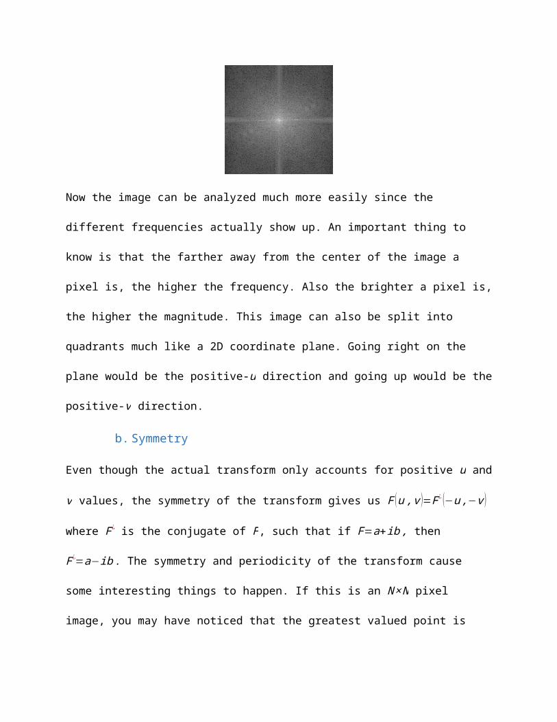
a. Logarithmic Scaling

In order for us to see the actual magnitude spectrum of the transform, it is necessary to apply a

logarithmic transformation to it. We can define a new form of the image as

Q (u , v )=c log (1+|F (u , v )|), where c is a scaling constant and is chosen depending on how many

different gray levels are available. The result of this transformation basically compresses the high

magnitude values into a relatively small range and at the same time, enhances the low magnitude

values. After the log transform of the above image, we obtain:

Now the image can be analyzed much more easily since the different frequencies actually show

up. An important thing to know is that the farther away from the center of the image a pixel is,

the higher the frequency. Also the brighter a pixel is, the higher the magnitude. This image can

also be split into quadrants much like a 2D coordinate plane. Going right on the plane would be

the positive-u direction and going up would be the positive-v direction.

b. Symmetry

Even though the actual transform only accounts for positive u and v values, the symmetry of the

transform gives us F (u , v )=F¿ (−u ,−v ) where F ¿ is the conjugate of F, such that if F=a+ib ,

then F ¿=a−ib . The symmetry and periodicity of the transform cause some interesting things to

happen. If this is an N ×N pixel image, you may have noticed that the greatest valued point is

roughly ( N2 ,N2 ), while the lowest valued point is (−N

2,−N

2 ). It turns out that, in the transform,

once we get past u=N2

and v=N2

, we start calculating the negative u and v values in the Fourier

domain. For instance, if N=16 , the frequency found at F (10,3) is actually the exact same value

of the frequency that would be found at F (−6 ,3), where a frequency with the same magnitude,

but an inverted shift (phase) would be found at F (6 ,−3). For this reason, any frequency F (u , v )

in the Fourier domain will have an identical looking frequency reflected over the origin of the

magnitude spectrum. As a result, this means that calculating F (10 ,3 ) automatically gives us the

magnitude of F (6 ,13 ) with an inverted phase, or F (u , v )=F¿ (N−u ,N−v ) . This is how

symmetry can be used to speed up the calculation process. To make sure this piece of

information is understood, let’s look at another transform:

The image on the right is the Fourier transformed image of the image on the left. Notice how the

origin is in the top left corner of both images. Due to the periodicity of the frequency domain,

any point beyond the line u=N2

or v=N2

(or both) is actually identical to a point on the opposite

side of the origin. This is why a a “quadrant swap” can be done to obtain:

This is the desired form of the transform since it displays an entire period with the origin at the

center of the image.

c. Magnitude and Phase

So, going back to the magnitude spectrum of the image with the clown,

Clearly, the image contains components of most frequencies, but the pixels get darker along the

edge of the image, indicating that the magnitude of higher frequencies is smaller than the

magnitude of lower frequencies. This tells us that most of the original image information is

defined by lower frequency components. At this point, the reader may be wondering what the

phase spectrum is used for, and what its significance is. The answer to that question is that,

although the phase spectrum can tell us a lot about the position of the frequencies in the original

image, it is hardly ever used in image processing since we’re mostly interested in the geometrical

structure. The significance of the phase spectrum comes into play when performing the inverse

DFT because both the magnitude and phase information are required to bring us back to the

original spatial domain. Here is what just the phase spectrum of the clown image looks like:

And here’s what the inverse of just the magnitude spectrum looks like:

This second image contains exactly the same frequencies and number of frequencies as the

original image, but it is obviously unrecognizable. This brings us to the conclusion that, while

the phase spectrum can be ignored in the Fourier domain, it can’t be completely ignored in image

processing because it does contain crucial information.

d. Convolution

To actually edit pictures in the Fourier domain, we can utilize a property of the Fourier

Transform that says it is distributive over addition. Due to this property, we can add the Fourier

domain magnitude spectra of two different images to produce a single image, and perform the

inverse DFT to yield an image that would be the same as if we had added the two spatial domain

images together directly. To illustrate this, let’s use an example.

Where the image on the left is the spatial domain image and the image on the right is the shifted

and scaled Fourier domain image. By the way, this is just a simple example, but the Fourier

domain image shows magnitudes going along the diagonal because that’s where the image

intensity changes the most in the spatial domain image. Let’s use another image to add to this

one.

Now let’s see what happens when we perform the inverse DFT on the addition of the two Fourier

domain images:

As you can see, the spatial domain image corresponding to the addition of the two Fourier

domain images shows the two spatial domain images added together. In fact, according to the

distributivity law, the final image is the same as if we had directly added the two spatial domain

images together in the first place. Therefore we could have done this operation in the spatial

domain first to yield the added Fourier domain image, however there is usually no practical

application to doing it in that order.

Mathematically speaking, this isn’t actually addition, but multiplication in the Fourier domain.

The property mentioned deals with convolution: convolution in the spatial domain is equivalent

to multiplication in the Fourier domain. The convolution operation of two functions (spatial

domain images in this case) yields a third function that expresses how the graph of one is

modified by the other. This is one of the most important properties of the Fourier Transform. The

Convolution Theorem sates that

F {f∗g }=k ∙F {f }∙ F {g }

Where F {f } is the Fourier Transform of f , ¿ is the convolution operator, and k is a constant that

depends on the normalization constant used in the Fourier Transform. In the above example, the

multiplication of the Fourier domain images could be represented as F {f } ∙F {g } where taking its

inverse would give f∗g, the two spatial domain images added together.

e. Filtering

Extending this idea, we can filter out unwanted frequencies from images in a relatively simple

way. Instead of using the convolution operator in the spatial domain, we can just multiply in the

Fourier domain. A few examples I will go over are low pass filtering, high pass filtering, and

noise removal.

i. Low Pass Filtering

Low pass filtering can be used to blur an image. It will simply define a circle of a certain radius

centered at the origin where only frequencies inside the circle will “pass” through it.

Here is another example of an image with its Fourier transformed image. We can filter out the

higher frequencies with a Fourier domain circle like this:

Multiplying this filter image by the Fourier domain image will produce another Fourier image

like this:

Then, applying the inverse transform on the new Fourier image will produce a new, blurred

spatial domain image:

Filtering out the higher frequencies from the Fourier domain image effectively gets rid of a lot of

the sharp edges in the picture, preserving only the broad, smooth regions. A smaller circle will

produce an image with more blur, and a larger circle will produce an image with less blur.

ii. High Pass Filtering

The converse of a low pass filter is called a high pass filter. This filter can be used for edge

detection in certain applications. Using the same Fourier domain image as with the low pass

filter example, we can choose to filter out smaller frequencies, and thus preserve only edges

where the brightness change is the greatest.

iii. Noise Removal

Noise removal works in a very similar way, only we need to know where the noise is at before

we filter it out.

In this example, the noise appears as the four star-like dots with one in each quadrant. We can

mask out these spikes of unwanted frequencies to obtain:

There are a plethora of more advanced uses for the Fourier Transform when it comes to image

processing, but these last three examples are just some of the basics so that the reader can get a

good understanding of what is actually happening.

XI. Conclusion

In conclusion, Jean-Baptiste Joseph Fourier used sines and cosines to represent continuous,

periodic functions to come up with a solution to the general heat equation. Since his discovery,

that idea has been expanded to represent non-periodic functions with what has come to be known

as the Fourier Transform. Even though the Continuous Fourier Transform works perfectly fine

for continuous signals, the Discrete Fourier Transform is preferred in image processing because

its input is a discrete signal which is represented with an image of pixels. Furthermore, the

DFT’s symmetrical properties can be utilized to yield the Fast Fourier Transform algorithm

which drastically reduces computation times in computers. With the magnitude/phase

representation of the DFT, we can separate their spectra to analyze the results. Shifting and

scaling the magnitude spectrum of the transform allows one full period centered at the origin to

be displayed in a single image. This new Fourier domain image can be edited and filtered in

certain ways to remove unwanted frequencies, which can be understood with the Convolution

Theorem. There exist many papers and websites describing Fourier Analysis in deeper detail,

and go beyond the scope of this paper. The interested reader should be directed to the references

page to find just a few of such sources.

References(2014, October 27). Retrieved from Dictionary.com: dictionary.reference.com

Acharya, T., & Ray, A. K. (2005). ImageProcessing:PrinciplesandApplications. John Wiley & Sons.

ComplexFormofFourierSeries. (2014). Retrieved from Math24.net: www.math24.net/complex-form-of-fourier-series.html

Fisher, R., Perkins, S., Walker, A., & Wolfart, E. (2003). FourierTransform. Retrieved from HIPR2: http://homepages.inf.ed.ac.uk/rbf/HIPR2/fourier.htm

Glynn, E. F. (2007, February 14). FourierAnalysisandImageProcessing. Retrieved from http://research.stowers-institute.org/efg/Report/FourierAnalysis.pdf

Hel-Or, Y. (2010, Spring). Image Processing (PowerPoint).

Konttinen, J., Pyka, P., & Kangas, M. (Retrieved 2014). Fourier Transform in Image Processing. Lappeenranta University of Technology.

Lehar, S. (n.d.). AnIntuitiveExplanationofFourierTheory. Retrieved from http://cns-alumni.bu.edu/~slehar/fourier/fourier.html

Patel, A. (2013, Spring). Fourier Transforms. PartialDifferentialEquations. Taber Hall, Jamestown College: Lecture.

Smith, J. O. (n.d.). MathematicsoftheDiscreteFourierTransform(DFT). Retrieved from DSP Related: www.dsprelated.com/dspbooks/mdft/

Tanja, H. C. (2007). AdvancedEngineeringMathematics:Volume2. I. K. International Pvt Ltd.

Vanderplas, J. (2013, August 28). UnderstandingtheFFTAlgorithm. Retrieved from Pythonic Perambulations: https://jakevdp.github.io/blog/2013/08/28/understanding-the-fft/

Wang, R. (2007, November 15). FourierAnalysisandImageProcessing. Retrieved from fourier.eng.hmc.edu: fourier.eng.hmc.edu/e101/lectures/image_processing/Image_Processing.html

Weinhaus, F. (2011, October 27). ImageMagickv6Examples--FourierTransforms. Retrieved from imagemagick.org: http://www.imagemagick.org/Usage/fourier/

Young, I. T., Gerbrands, J. J., & van Vliet, L. J. (2007). Fundamentals of Image Processing. Delft University of Technology.