FPGA IMPLEMENTATIONS OF NEURAL...

FPGA IMPLEMENTATIONS OF NEURAL NETWORKS

FPGA Implementations of Neural Networks

Edited by

AMOS R. OMONDIFlinders University, Adelaide,SA, Australia

and

JAGATH C. RAJAPAKSENanyang Tecnological University,Singapore

A C.I.P. Catalogue record for this book is available from the Library of Congress.

ISBN-10 0-387-28485-0 (HB)ISBN-13 978-0-387-28485-9 (HB)ISBN-10 0-387-28487-7 ( e-book)ISBN-13 978-0-387-28487-3 (e-book)

Published by Springer,P.O. Box 17, 3300 AA Dordrecht, The Netherlands.

Printed on acid-free paper

All Rights Reserved

No part of this work may be reproduced, stored in a retrieval system, or transmittedin any form or by any means, electronic, mechanical, photocopying, microfilming, recordingor otherwise, without written permission from the Publisher, with the exceptionof any material supplied specifically for the purpose of being enteredand executed on a computer system, for exclusive use by the purchaser of the work.

Printed in the Netherlands.

www.springer.com

© 200 Springer 6

Contents

Preface ix

1FPGA Neurocomputers 1Amos R. Omondi, Jagath C. Rajapakse and Mariusz Bajger

1.1. Introduction 11.2. Review of neural-network basics 31.3. ASIC vs. FPGA neurocomputers 91.4. Parallelism in neural networks 121.5. Xilinx Virtex-4 FPGA 131.6. Arithmetic 151.7. Activation-function implementation: unipolar sigmoid 211.8. Performance evaluation 321.9. Conclusions 34References 34

237

Medhat Moussa and Shawki Areibi and Kristian Nichols2.1. Introduction 372.2. Background 392.3. Architecture design and implementation 432.4. Experiments using logical-XOR problem 482.5. Results and discussion 502.6. Conclusions 55References 56

3FPNA: Concepts and properties 63Bernard Girau

3.1. Introduction 633.2. Choosing FPGAs 653.3. FPNAs, FPNNs 713.4. Correctness 863.5. Underparameterized convolutions by FPNNs 883.6. Conclusions 96References 97

Arithmetic precision for implementing BP networks on FPGA: A case study

v

vi

4FPNA: Applications and implementations 103Bernard Girau

4.1. Summary of Chapter 3 1044.2. Towards simplified architectures: symmetric boolean functions by

FPNAs 1054.3. Benchmark applications 1094.4. Other applications 1134.5. General FPGA implementation 1164.6. Synchronous FPNNs 1204.7. Implementations of synchronous FPNNs 1244.8. Implementation performances 1304.9. Conclusions 133References 134

5Back-Propagation Algorithm Achieving 5 GOPS on the Virtex-E 137Kolin Paul and Sanjay Rajopadhye

5.1. Introduction 1385.2. Problem specification 1395.3. Systolic implementation of matrix-vector multiply 1415.4. Pipelined back-propagation architecture 1425.5. Implementation 1445.6. MMAlpha design environment 1475.7. Architecture derivation 1495.8. Hardware generation 1555.9. Performance evaluation 1575.10. Related work 1595.11. Conclusion 160Appendix 161References 163

6FPGA Implementation of Very Large Associative Memories 167Dan Hammerstrom, Changjian Gao, Shaojuan Zhu, Mike Butts

6.1. Introduction 1676.2. Associative memory 1686.3. PC Performance Evaluation 1796.4. FPGA Implementation 1846.5. Performance comparisons 1906.6. Summary and conclusions 192References 193

7FPGA Implementations of Neocognitrons 197Alessandro Noriaki Ide and José Hiroki Saito

7.1. Introduction 1977.2. Neocognitron 1987.3. Alternative neocognitron 2017.4. Reconfigurable computer 2057.5. Reconfigurable orthogonal memory multiprocessor 206

FPGA Implementations of neural networks

Contents vii

7.6. Alternative neocognitron hardware implementation 2097.7. Performance analysis 2157.8. Applications 2187.9. Conclusions 221References 222

8Self Organizing Feature Map for Color Quantization on FPGA 225Chip-Hong Chang, Menon Shibu and Rui Xiao

8.1. Introduction 2258.2. Algorithmic adjustment 2288.3. Architecture 2318.4. Implementation 2358.5. Experimental results 2398.6. Conclusions 242References 242

9Implementation of Self-Organizing Feature Maps in Reconfigurable

Hardware247

Mario Porrmann, Ulf Witkowski, and Ulrich Rückert9.1. Introduction 2479.2. Using reconfigurable hardware for neural networks 2489.3. The dynamically reconfigurable rapid prototyping system

RAPTOR2000 2509.4. Implementing self-organizing feature maps on RAPTOR2000 2529.5. Conclusions 267References 267

10FPGA Implementation of a Fully and Partially Connected MLP 271

Antonio Canas, Eva M. Ortigosa, Eduardo Ros and Pilar M. Ortigosa10.1. Introduction 27110.2. MLP/XMLP and speech recognition 27310.3. Activation functions and discretization problem 27610.4. Hardware implementations of MLP 28410.5. Hardware implementations of XMLP 29110.6. Conclusions 293Acknowledgments 294References 295

11FPGA Implementation of Non-Linear Predictors 297Rafael Gadea-Girones and Agustn Ramrez-Agundis

11.1. Introduction 29811.2. Pipeline and back-propagation algorithm 29911.3. Synthesis and FPGAs 30411.4. Implementation on FPGA 31311.5. Conclusions 319References 321

viii

12The REMAP reconfigurable architecture: a retrospective 325Lars Bengtsson, Arne Linde, Tomas Nordstr-om, Bertil Svensson,and Mikael Taveniku

12.1. Introduction 32612.2. Target Application Area 32712.3. REMAP-β – design and implementation 33512.4. Neural networks mapped on REMAP-β 34612.5. REMAP- γ architecture 35312.6. Discussion 35412.7. Conclusions 357Acknowledgments 357References 357


Preface

During the 1980s and early 1990s there was significant work in the designand implementation of hardware neurocomputers. Nevertheless, most of theseefforts may be judged to have been unsuccessful: at no time have have hard-ware neurocomputers been in wide use. This lack of success may be largelyattributed to the fact that earlier work was almost entirely aimed at developingcustom neurocomputers, based on ASIC technology, but for such niche ar-eas this technology was never sufficiently developed or competitive enough tojustify large-scale adoption. On the other hand, gate-arrays of the period men-tioned were never large enough nor fast enough for serious artificial-neural-network (ANN) applications. But technology has now improved: the capacityand performance of current FPGAs are such that they present a much morerealistic alternative. Consequently neurocomputers based on FPGAs are nowa much more practical proposition than they have been in the past. This booksummarizes some work towards this goal and consists of 12 papers that wereselected, after review, from a number of submissions. The book is nominallydivided into three parts: Chapters 1 through 4 deal with foundational issues;Chapters 5 through 11 deal with a variety of implementations; and Chapter12 looks at the lessons learned from a large-scale project and also reconsidersdesign issues in light of current and future technology.

Chapter 1 reviews the basics of artificial-neural-network theory, discussesvarious aspects of the hardware implementation of neural networks (in bothASIC and FPGA technologies, with a focus on special features of artificialneural networks), and concludes with a brief note on performance-evaluation.Special points are the exploitation of the parallelism inherent in neural net-works and the appropriate implementation of arithmetic functions, especiallythe sigmoid function. With respect to the sigmoid function, the chapter in-cludes a significant contribution.

Certain sequences of arithmetic operations form the core of neural-networkcomputations, and the second chapter deals with a foundational issue: howto determine the numerical precision format that allows an optimum tradeoffbetween precision and implementation (cost and performance). Standard sin-gle or double precision floating-point representations minimize quantization

ix

x

errors while requiring significant hardware resources. Less precise fixed-pointrepresentation may require less hardware resources but add quantization errorsthat may prevent learning from taking place, especially in regression problems.Chapter 2 examines this issue and reports on a recent experiment where we im-plemented a multi-layer perceptron on an FPGA using both fixed and floatingpoint precision.

A basic problem in all forms of parallel computing is how best to map ap-plications onto hardware. In the case of FPGAs the difficulty is aggravatedby the relatively rigid interconnection structures of the basic computing cells.Chapters 3 and 4 consider this problem: an appropriate theoretical and prac-tical framework to reconcile simple hardware topologies with complex neuralarchitectures is discussed. The basic concept is that of Field ProgrammableNeural Arrays (FPNA) that lead to powerful neural architectures that are easyto map onto FPGAs, by means of a simplified topology and an original dataexchange scheme. Chapter 3 gives the basic definition and results of the theo-retical framework. And Chapter 4 shows how FPNAs lead to powerful neuralarchitectures that are easy to map onto digital hardware. applications and im-plementations are described, focusing on a class

Chapter 5 presents a systolic architecture for the complete back propagationalgorithm. This is the first such implementation of the back propagation algo-rithm which completely parallelizes the entire computation of learning phase.The array has been implemented on an Annapolis FPGA based coprocessorand it achieves very favorable performance with range of 5 GOPS. The pro-posed new design targets Virtex boards. A description is given of the process ofautomatically deriving these high performance architectures using the systolicarray design tool MMAlpha, facilitates system-specification This makes iteasy to specify the system in a very high level language (Alpha) and alsoallows perform design exploration to obtain architectures whose performanceis comparable to that obtained using hand optimized VHDL code.

Associative networks have a number of properties, including a rapid, com-pute efficient best-match and intrinsic fault tolerance, that make them ideal formany applications. However, large networks can be slow to emulate becauseof their storage and bandwidth requirements. Chapter 6 presents a simple buteffective model of association and then discusses a performance analysis of theimplementation this model on a single high-end PC workstation, a PC cluster,and FPGA hardware.

Chapter 7 describes the implementation of an artificial neural network in areconfigurable parallel computer architecture using FPGA’s, named Reconfig-urable Orthogonal Memory Multiprocessor (REOMP), which uses p2 memorymodules connected to p reconfigurable processors, in row access mode, andcolumn access mode. REOMP is considered as an alternative model of theneural network neocognitron. The chapter consists of a description of the RE-


xi

OMP architecture, a the case study of alternative neocognitron mapping, and aperformance performance analysis with systems systems consisting of 1 to 64processors.

Chapter 8 presents an efficient architecture of Kohonen Self-OrganizingFeature Map (SOFM) based on a new Frequency Adaptive Learning (FAL)algorithm which efficiently replaces the neighborhood adaptation function ofthe conventional SOFM. The proposed SOFM architecture is prototyped onXilinx Virtex FPGA using the prototyping environment provided by XESS.A robust functional verification environment is developed for rapid prototypedevelopment. Various experimental results are given for the quantization of a512 X 512 pixel color image.

Chapter 9 consists of another discussion of an implementation of SOFMsin reconfigurable hardware. Based on the universal rapid prototyping system,RAPTOR2000, a hardware accelerator for self-organizing feature maps hasbeen developed. Using Xilinx Virtex-E FPGAs, RAPTOR2000 is capable ofemulating hardware implementations with a complexity of more than 15 mil-lion system gates. RAPTOR2000 is linked to its host – a standard personalcomputer or workstation – via the PCI bus. A speed-up of up to 190 is achievedwith five FPGA modules on the RAPTOR2000 system compared to a softwareimplementation on a state of the art personal computer for typical applicationsof SOFMs.

Chapter 10 presents several hardware implementations of a standard Multi-Layer Perceptron (MLP) and a modified version called eXtended Multi-LayerPerceptron (XMLP). This extended version is an MLP-like feed-forward net-work with two-dimensional layers and configurable connection pathways. Thediscussion includes a description of hardware implementations have been de-veloped and tested on an FPGA prototyping board and includes systems spec-ifications using two different abstraction levels: register transfer level (VHDL)and a higher algorithmic-like level (Handel-C) as well as the exploitation ofvarying degrees of parallelism. The main test bed application is speech recog-nition.

Chapter 11 describes the implementation of a systolic array for a non-linearpredictor for image and video compression. The implementation is based on amultilayer perceptron with a hardware-friendly learning algorithm. It is shownthat even with relatively modest FPGA devices, the architecture attains thespeeds necessary for real-time training in video applications and enabling moretypical applications to be added to the image compression processing

The final chapter consists of a retrospective look at the REMAP project,which was the construction of design, implementation, and use of large-scaleparallel architectures for neural-network applications. The chapter gives anoverview of the computational requirements found in algorithms in general andmotivates the use of regular processor arrays for the efficient execution of such

Preface

xii

algorithms. The architecture, following the SIMD principle (Single Instruc-tion stream, Multiple Data streams), is described, as well as the mapping ofsome important and representative ANN algorithms. Implemented in FPGA,the system served as an architecture laboratory. Variations of the architectureare discussed, as well as scalability of fully synchronous SIMD architectures.The design principles of a VLSI-implemented successor of REMAP-β are de-scribed, and the paper concludes with a discussion of how the more powerfulFPGA circuits of today could be used in a similar architecture.

AMOS R. OMONDI AND JAGATH C. RAJAPAKSE


Chapter 1

FPGA NEUROCOMPUTERS

Amos R. OmondiSchool of Informatics and Engineering, Flinders University, Bedford Park, SA 5042, Australia

[email protected]

Jagath C. RajapakseSchool Computer Engineering, Nanyang Technogoical University, Singapore 639798

[email protected]

Mariusz BajgerSchool of Informatics and Engineering, Flinders University, Bedford Park, SA 5042, Australia

[email protected]

AbstractThis introductory chapter reviews the basics of artificial-neural-network the-

ory, discusses various aspects of the hardware implementation of neural net-works (in both ASIC and FPGA technologies, with a focus on special featuresof artificial neural networks), and concludes with a brief note on performance-evaluation. Special points are the exploitation of the parallelism inherent inneural networks and the appropriate implementation of arithmetic functions, es-pecially the sigmoid function. With respect to the sigmoid function, the chapterincludes a significant contribution.

Keywords: FPGAs, neurocomputers, neural-network arithmetic, sigmoid, performance-evaluation.

1.1 Introduction

In the 1980s and early 1990s, a great deal of research effort (both industrialand academic) was expended on the design and implementation of hardwareneurocomputers [5, 6, 7, 8]. But, on the whole, most efforts may be judged

1

A. R. Omondi and J. C. Rajapakse (eds.), FPGA Implementations of Neural Networks, 1–36. © 2006 Springer. Printed in the Netherlands.

2 FPGA Neurocomputers

to have been unsuccessful: at no time have have hardware neurocomputersbeen in wide use; indeed, the entire field was largely moribund by the end the1990s. This lack of success may be largely attributed to the fact that earlierwork was almost entirely based on ASIC technology but was never sufficientlydeveloped or competetive enough to justify large-scale adoption; gate-arraysof the period mentioned were never large enough nor fast enough for seriousneural-network applications.1 Nevertheless, the current literature shows thatASIC neurocomputers appear to be making some sort of a comeback [1, 2, 3];we shall argue below that these efforts are destined to fail for exactly the samereasons that earlier ones did. On the other hand, the capacity and performanceof current FPGAs are such that they present a much more realistic alternative.We shall in what follows give more detailed arguments to support these claims.

The chapter is organized as follows. Section 2 is a review of the fundamen-tals of neural networks; still, it is expected that most readers of the book will al-ready be familiar with these. Section 3 briefly contrasts ASIC-neurocomputerswith FPGA-neurocomputers, with the aim of presenting a clear case for theformer; a more significant aspects of this argument will be found in [18]. Oneof the most repeated arguments for implementing neural networks in hardwareis the parallelism that the underlying models possess. Section 4 is a short sec-tion that reviews this. In Section 5 we briefly describe the realization of astate-of-the art FPGA device. The objective there is to be able to put into aconcrete context certain following discussions and to be able to give groundeddiscussions of what can or cannot be achieved with current FPGAs. Section6 deals with certain aspects of computer arithmetic that are relevant to neural-network implementations. Much of this is straightforward, and our main aimis to highlight certain subtle aspects. Section 7 nominally deals with activa-tion functions, but is actually mostly devoted to the sigmoid function. Thereare two main reasons for this choice: first, the chapter contains a significantcontribution to the implementation of elementary or near-elementary activa-tion functions, the nature of which contribution is not limited to the sigmoidfunction; second, the sigmoid function is the most important activation func-tion for neural networks. In Section 8, we very briefly address an importantissue — performance evaluation. Our goal here is simple and can be statedquite succintly: as far as performance-evaluation goes, neurocomputer archi-tecture continues to languish in the “Dark Ages", and this needs to change. Afinal section summarises the main points made in chapter and also serves as abrief introduction to subsequent chapters in the book.

1Unless otherwise indicated, we shall use neural network to mean artificial neural network.

Review of neural-network basics 3

1.2 Review of neural-network basics

The human brain, which consists of approximately 100 billion neurons thatare connected by about 100 trillion connections, forms the most complex objectknown in the universe. Brain functions such as sensory information process-ing and cognition are the results of emergent computations carried out by thismassive neural network. Artificial neural networks are computational modelsthat are inspired by the principles of computations performed by the biolog-ical neural networks of the brain. Neural networks possess many attractivecharacteristics that may ultimately surpass some of the limitations in classicalcomputational systems. The processing in the brain is mainly parallel and dis-tributed: the information are stored in connections, mostly in myeline layersof axons of neurons, and, hence, distributed over the network and processed ina large number of neurons in parallel. The brain is adaptive from its birth to itscomplete death and learns from exemplars as they arise in the external world.Neural networks have the ability to learn the rules describing training data and,from previously learnt information, respond to novel patterns. Neural networksare fault-tolerant, in the sense that the loss of a few neurons or connections doesnot significantly affect their behavior, as the information processing involvesa large number of neurons and connections. Artificial neural networks havefound applications in many domains — for example, signal processing, imageanalysis, medical diagnosis systems, and financial forecasting.

The roles of neural networks in the afore-mentioned applications fallbroadly into two classes: pattern recognition and functional approximation.The fundamental objective of pattern recognition is to provide a meaningfulcategorization of input patterns. In functional approximation, given a set ofpatterns, the network finds a smooth function that approximates the actualmapping between the input and output.

A vast majority of neural networks are still implemented on software onsequential machines. Although this is not necessarily always a severe limita-tion, there is much to be gained from directly implementing neual networksin hardware, especially if such implementation exploits the parellelism inher-ent in the neural networks but without undue costs. In what follows, we shalldescribe a few neural network models — multi-layer perceptrons, Kohonen’sself-organizing feature map, and associative memory networks — whose im-plementations on FPGA are discussed in the other chapters of the book.

1.2.1 Artificial neuron

An artificial neuron forms the basic unit of artficial neural networks. Thebasic elements of an artificial neurons are (1) a set of input nodes, indexed by,say, 1, 2, ... I , that receives the corresponding input signal or pattern vector,say x = (x1, x2, . . . xI)T; (2) a set of synaptic connections whose strengths are


represented by a set of weights, here denoted by w = (w1, w2, . . . wI)T; and(3) an activation function Φ that relates the total synaptic input to the output(activation) of the neuron. The main components of an artificial neuron isillustrated in Figure 1.

Figure 1: The basic components of an artificial neuron

The total synaptic input, u, to the neuron is given by the inner product of theinput and weight vectors:

u =I∑

i=1

wixi (1.1)

where we assume that the threshold of the activation is incorporated in theweight vector. The output activation, y, is given by

y = Φ(u) (1.2)

where Φ denotes the activation function of the neuron. Consequently, the com-putation of the inner-products is one of the most important arithmetic opera-tions to be carried out for a hardware implementation of a neural network. Thismeans not just the individual multiplications and additions, but also the alterna-tion of successive multiplications and additions — in other words, a sequenceof multiply-add (also commonly known as multiply-accumulate or MAC) op-erations. We shall see that current FPGA devices are particularly well-suitedto such computations.

The total synaptic input is transformed to the output via the non-linear acti-vation function. Commonly employed activation functions for neurons are


the threshold activation function (unit step function or hard limiter):

Φ(u) ={

1.0, when u > 0,0.0, otherwise.

the ramp activation function:2

Φ(u) = max {0.0, min{1.0, u + 0.5}}

the sigmodal activation function, where the unipolar sigmoid function is

Φ(u) =a

1 + exp(−bu)

and the bipolar sigmoid is

Φ(u) = a

(1 − exp(−bu)1 + exp(−bu)

)where a and b represent, repectively, real constants the gain or amplitudeand the slope of the transfer function.

The second most important arithmetic operation required for neural networksis the computation of such activation functions. We shall see below that thestructure of FPGAs limits the ways in which these operations can be carriedout at reasonable cost, but current FPGAs are also equipped to enable high-speed implementations of these functions if the right choices are made.

A neuron with a threshold activation function is usually referred to as thediscrete perceptron, and with a continuous activation function, usually a sig-moidal function, such a neuron is referred to as continuous perceptron. Thesigmoidal is the most pervasive and biologically plausible activation function.

Neural networks attain their operating characteristics through learning ortraining. During training, the weights (or strengths) of connections are gradu-ally adjusted in either supervised or unsupervised manner. In supervised learn-ing, for each training input pattern, the network is presented with the desiredoutput (or a teacher), whereas in unsupervised learning, for each training inputpattern, the network adjusts the weights without knowing the correct target.The network self-organizes to classify similar input patterns into clusters inunsupervised learning. The learning of a continuous perceptron is by adjust-ment (using a gradient-descent procedure) of the weight vector, through theminimization of some error function, usually the square-error between the de-sired output and the output of the neuron. The resultant learning is known as

2In general, the slope of the ramp may be other than unity.


as delta learning: the new weight-vector, wnew, after presentation of an inputx and a desired output d is given by

wnew = wold + αδx

where wold refers to the weight vector before the presentation of the input andthe error term, δ, is (d − y)Φ′(u), where y is as defined in Equation 1.2 andΦ

′is the first derivative of Φ. The constant α, where 0 < α ≤ 1, denotes the

learning factor. Given a set of training data, Γ = {(xi, di); i = 1, . . . n}, thecomplete procedure of training a continuous perceptron is as follows:

begin: /* training a continuous perceptron */Initialize weights wnew

RepeatFor each pattern (xi, di) do

wold = wnew

wnew = wold + αδxi

until convergenceend

The weights of the perceptron are initialized to random values, and the conver-gence of the above algorithm is assumed to have been achieved when no moresignificant changes occur in the weight vector.

1.2.2 Multi-layer perceptron

The multi-layer perceptron (MLP) is a feedforward neural network consist-ing of an input layer of nodes, followed by two or more layers of perceptrons,the last of which is the output layer. The layers between the input layer andoutput layer are referred to as hidden layers. MLPs have been applied success-fully to many complex real-world problems consisting of non-linear decisionboundaries. Three-layer MLPs have been sufficient for most of these applica-tions. In what follows, we will briefly describe the architecture and learning ofan L-layer MLP.

Let 0-layer and L-layer represent the input and output layers, respectively;and let wl+1

kj denote the synaptic weight connected to the k-th neuron of thel + 1 layer from the j-th neuron of the l-th layer. If the number of perceptrons

in the l-th layer is Nl, then we shall let Wl�= {wl

kj}NlxNl−1denote the matrix

of weights connecting to l-th layer. The vector of synaptic inputs to the l-thlayer, ul = (ul

1, ul2, . . . u

lNl

)T is given by

ul = Wlyl−1,

where yl−1 = (yl−11 , yl−1

2 , . . . yl−1Nl−1

)T denotes the vector of outputs at the l−1layer. The generalized delta learning-rule for the layer l is, for perceptrons,


given by

Wnewl = Wold

l + αδ lyTl−1,

where the vector of error terms, δ Tl = (δl

1, δl2, . . . , δ

lNl

) at the l th layer isgiven by

δlj =

{2Φl

j′(ul

j)(dj − oj), when l = L,

Φlj′(ul

j)∑Nl+1

k=1 δl+1k wl+1

kj , otherwise,

where oj and dj denote the network and desired outputs of the j-th outputneuron, respectively; and Φl

j and ulj denote the activation function and total

synaptic input to the j-th neuron at the l-th layer, respectively. During train-ing, the activities propagate forward for an input pattern; the error terms of aparticular layer are computed by using the error terms in the next layer and,hence, move in the backward direction. So, the training of MLP is referred aserror back-propagation algorithm. For the rest of this chapter, we shall gen-eraly focus on MLP networks with backpropagation, this being, arguably, themost-implemented type of artificial neural networks.

Figure 2: Architecture of a 3-layer MLP network


1.2.3 Self-organizing feature maps

Neurons in the cortex of the human brain are organized into layers of neu-rons. These neurons not only have bottom-up and top-down connections, butalso have lateral connections. A neuron in a layer excites its closest neigh-bors via lateral connections but inhibits the distant neighbors. Lateral inter-actions allow neighbors to partially learn the information learned by a winner(formally defined below), which gives neighbors responding to similar pat-terns after learning with the winner. This results in topological ordering offormed clusters. The self-organizing feature map (SOFM) is a two-layer self-organizing network which is capable of learning input patterns in a topolog-ically ordered manner at the output layer. The most significant concept in alearning SOFM is that of learning within a neighbourhood around a winningneuron. Therefore not only the weights of the winner but also those of theneighbors of the winner change.

The winning neuron, m, for an input pattern x is chosen according to thetotal synaptic input:

m = arg maxj

wTj x,

where wj denotes the weight-vector corresponding to the j-th output neuron.wT

mx determines the neuron with the shortest Euclidean distance between itsweight vector and the input vector when the input patterns are normalized tounity before training.

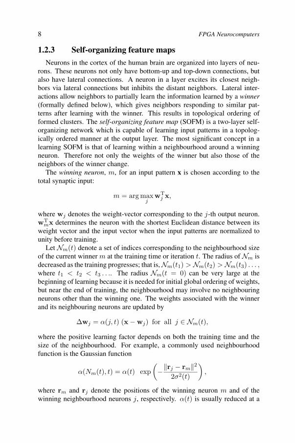
Let Nm(t) denote a set of indices corresponding to the neighbourhood sizeof the current winner m at the training time or iteration t. The radius of Nm isdecreased as the training progresses; that is, Nm(t1) > Nm(t2) > Nm(t3) . . . ,where t1 < t2 < t3 . . .. The radius Nm(t = 0) can be very large at thebeginning of learning because it is needed for initial global ordering of weights,but near the end of training, the neighbourhood may involve no neighbouringneurons other than the winning one. The weights associated with the winnerand its neighbouring neurons are updated by

∆wj = α(j, t) (x − wj) for all j ∈ Nm(t),

where the positive learning factor depends on both the training time and thesize of the neighbourhood. For example, a commonly used neighbourhoodfunction is the Gaussian function

α(Nm(t), t) = α(t) exp(−‖rj − rm‖2

2σ2(t)

),

where rm and rj denote the positions of the winning neuron m and of thewinning neighbourhood neurons j, respectively. α(t) is usually reduced at a

ASIC vs. FPGA neurocomputers 9

rate that is inversely proportional to t. The type of training described aboveis known as Kohonen’s algorithm (for SOFMs). The weights generated by theabove algorithms are arranged spatially in an ordering that is related to thefeatures of the trained patterns. Therefore, the algorithm produces topology-preserving maps. After learning, each input causes a localized response withpositions on the output layer that reflects dominant features of the input.

1.2.4 Associative-memory networks

Associative memory networks are two-layer networks in which weightsare determined in order to store a set of pattern associations, say,{(s1, t1), (s2, t2), . . . (sk, tk), . . . (sn, tn)}, where input pattern sk is associ-ated with output pattern tk. These networks not only learn to produce asso-ciative patterns, but also are able to recall the desired response patterns whena given pattern is similar to the stored pattern. Therefore they are referredto as content-addressible memory. For each association vector (sk, tk), ifsk = tk, the network is referred to as auto-associative; otherwise it is hetero-associative. The networks often provide input-output descriptions of the asso-ciative memory through a linear transformation (then known as linear associa-tive memory). The neurons in these networks have linear activation functions.If the linearity constant is unity, then the output layer activation is given by

y = Wx,

where W denotes the weight matrix connecting the input and output layers.These networks learn using the Hebb rule; the weight matrix to learn all theassociations is given by the batch learning rule:

W =n∑

k=1

tksTk .

If the stored patterns are orthogonal to each other, then it can be shown thatthe network recalls the stored associations perfectly. Otherwise, the recalledpatterns are distorted by cross-talk between patterns.

1.3 ASIC vs. FPGA neurocomputers

By far, the most often-stated reason for the development of custom (i.e.ASIC) neurocomputers is that conventional (i.e. sequential) general-purposeprocessors do not fully exploit the parallelism inherent in neural-network mod-els and that highly parallel architectures are required for that. That is true asfar as it goes, which is not very far, since it is mistaken on two counts [18]:The first is that it confuses the final goal, which is high performance — notmerely parallelism — with artifacts of the basic model. The strong focus on


parallelism can be justified only when high performance is attained at a rea-sonable cost. The second is that such claims ignore the fact that conventionalmicroprocessors, as well as other types of processors with a substantial user-base, improve at a much faster rate than (low-use) special-purpose ones, whichimplies that the performance (relative to cost or otherwise) of ASIC neurocom-puters will always lag behind that of mass-produced devices – even on specialapplications. As an example of this misdirection of effort, consider the latestin ASIC neurocomputers, as exemplified by, say, [3]. It is claimed that “withrelatively few neurons, this ANN-dedicated hardware chip [Neuricam Totem]outperformed the other two implementations [a Pentium-based PC and a TexasInstruments DSP]”. The actual results as presented and analysed are typicalof the poor benchmarking that afflicts the neural-network area. We shall havemore to say below on that point, but even if one accepts the claims as given,some remarks can be made immediately. The strongest performance-claimmade in [3], for example, is that the Totem neurochip outperformed, by a fac-tor of about 3, a PC (with a 400-MHz Pentium II processor, 128 Mbytes ofmain memory, and the neural netwoks implemented in Matlab). Two pointsare pertinent here:

In late-2001/early 2002, the latest Pentiums had clock rates that weremore than 3 times that of Pentium II above and with much more memory(cache, main, etc.) as well.

The PC implementation was done on top of a substantial software (base),instead of a direct low-level implementation, thus raising issues of “best-effort” with respect to the competitor machines.

A comparison of the NeuriCam Totems and Intel Pentiums, in the years 2002and 2004 will show the large basic differences have only got larger, primarilybecause, with the much large user-base, the Intel (x86) processors continue toimprove rapidly, whereas little is ever heard of about the neurocomputers asPCs go from one generation to another.

So, where then do FGPAs fit in? It is evident that in general FPGAs can-not match ASIC processors in performance, and in this regard FPGAs havealways lagged behind conventional microprocessors. Nevertheless, if oneconsiders FPGA structures as an alternative to software on, say, a general-purpose processor, then it is possible that FPGAs may be able to deliver bettercost:performance ratios on given applications.3 Moreover, the capacity forreconfiguration means that may be extended to a range of applications, e.g.several different types of neural networks. Thus the main advantage of theFPGA is that it may offer a better cost:performance ratio than either custom

3Note that the issue is cost:performance and not just performance

ASIC vs. FPGA neurocomputers 11

ASIC neurocomputers or state-of-the art general-purpose processors and withmore flexibility than the former. A comparison of the NeuriCam Totem, In-tel Pentiums, and M FPGAs will also show that improvements that show theadvantages of of the FPGAs, as a consequence of relatively rapid changes indensity and speed.

It is important to note here two critical points in relation to custom (ASIC)neurocomputers versus the FPGA structures that may be used to implement avariety of artificial neural networks. The first is that if one aims to realize a cus-tom neurocomputer that has a signficiant amount of flexibility, then one endsup with a structure that resembles an FPGA — that is, a small number of differ-ent types functional units that can be configured in different ways, according tothe neural network to be implemented — but which nonetheless does not havethe same flexibility. (A particular aspect to note here is that the large variety ofneural networks — usually geared towards different applications — gives risea requirement for flexibility, in the form of either programmability or recon-figurability.) The second point is that raw hardware-performance alone doesnot constitute the entirety of a typical computing structure: software is alsorequired; but the development of software for custom neurocomputers will,because of the limited user-base, always lag behind that of the more widelyused FPGAs. A final drawback of the custom-neurocomputer approach is thatmost designs and implementations tend to concentrate on just the high paral-lelism of the neural networks and generally ignore the implications of Am-dahl’s Law, which states that ultimately the speed-up will be limited by anyserial or lowly-parallel processing involved. (One rare exception is [8].)4 Thusnon-neural and other serial parts of processing tend to be given short shrift.Further, even where parallelism can be exploited, most neurocomputer-designseem to to take little account of the fact that the degrees of useful parallelismwill vary according to particular applications. (If parallelism is the main is-sue, then all this would suggest that the ideal building block for an appropri-ate parallel-processor machine is one that is less susceptible to these factors,and this argues for a relatively large-grain high-performance processor, used insmaller numbers, that can nevertheless exploit some of the parallelism inherentin neural networks [18].)

All of the above can be summed up quite succintly: despite all the claimsthat have been made and are still being made, to date there has not been acustom neurocomputer that, on artificial neural-network problems (or, for thatmatter, on any other type of problem), has outperformed the best conventionalcomputer of its time. Moreover, there is little chance of that happening. The

4Although not quite successful as a neurocomputer, this machine managed to survive longer than mostneurocomputers — because the flexibility inherent in its design meant that it could also be useful for non-neural applications.


promise of FPGAs is that they offer, in essence, the ability to realize “semi-custom” machines for neural networks; and, with continuing developments intechnology, they thus offer the best hope for changing the situation, as far aspossibly outperforming (relative to cost) conventional processors.

1.4 Parallelism in neural networks

Neural networks exhibit several types of parallelism, and a careful examina-tion of these is required in order to both determine the most suitable hardwarestructures as well as the best mappings from the neural-network structures ontogiven hardware structures. For example, parallelism can be of the SIMD typeor of the MIMD type, bit-parallel or word-parallel, and so forth [5]. In general,the only categorical statement that can be made is that, except for networks of atrivial size, fully parallel implementation in hardware is not feasible — virtualparallelism is necessary, and this, in turn, implies some sequential processing.In the context of FPGa, it might appear that reconfiguration is a silver bullet,but this is not so: the benefits of dynamic reconfigurability must be evaluatedrelative to the costs (especially in time) of reconfiguration. Nevertheless, thereis litle doubt that FPGAs are more promising that ASIC neurocomputers. Thespecific types of parallelism are as follows.

Training parallelism: Different training sessions can be run in parallel,e.g. on SIMD or MIMD processors. The level of parallelism at this levelis usually medium (i.e. in the hundreds), and hence can be nearly fullymapped onto current large FPGAs.

Layer parallelism: In a multilayer network, different layers can beprocessed in parallel. Parallelism at this level is typically low (in thetens), and therefore of limited value, but it can still be exploited throughpipelining.

Node parallelism: This level, which coresponds to individual neurons, isperhaps the most important level of parallelism, in that if fully exploited,then parallelism at all of the above higher levels is also fully exploited.But that may not be possible, since the number of neurons can be ashigh as in the millions. Nevertheless, node parallelism matches FPGAsvery well, since a typical FPGA basically consists of a large number of“cells” that can operate in parallel and, as we shall see below, onto whichneurons can readily be mapped.

Weight parallelism: In the computation of an output

y = Φ

(n∑

i=1

wixi

),

Xilinx Virtex-4 FPGA 13

where xi is an input and wi is a weight, the products xiwi can all becomputed in parallel, and the sum of these products can also be com-puted with high parallelism (e.g. by using an adder-tree of logarithmicdepth).

Bit-level parallelism: At the implementation level, a wide variety of par-allelism is available, depending on the design of individual functionalunits. For example, bit-serial, serial-parallel, word-parallel, etc.

From the above, three things are evident in the context of an implementation.First, the parallelism available at the different levels varies enormously. Sec-ond, different types of parallelism may be traded off against others, dependingon the desired cost:performance ratio (where for an FPGA cost may be mea-sured in, say, the number of CLBs etc.); for example, the slow speed of asingle functional unit may be balanced by having many such units operatingconcurrently. And third, not all types of parallelism are suitable for FPGAimplementation: for example, the required routing-interconnections may beproblematic, or the exploitation of bit-level parallelism may be constrained bythe design of the device, or bit-level parallelism may simply not be appropriate,and so forth. In the Xilinx Virtex-4, for example, we shall see that it is possibleto carry out many neural-network computations without using much of what isusually taken as FPGA fabric.5

1.5 Xilinx Virtex-4 FPGA

In this section, we shall briefly give the details an current FPGA device,the Xilinx Virtex-4, that is typical of state-of-the-art FPGA devices. We shallbelow use this device in several running examples, as these are easiest under-stood in the context of a concrete device. The Virtex-4 is actually a family ofdevices with many common features but varying in speed, logic-capacity, etc..The Virtex-E consists of an array of up to 192-by-116 tiles (in generic FPGAterms, configurable logic blocks or CLBs), up to 1392 Kb of Distributed-RAM,upto 9936 Kb of Block-RAM (arranged in 18-Kb blocks), up to 2 PowerPC 405processors, up to 512 Xtreme DSP slices for arithmetic, input/ouput blocks,and so forth.6

A tile is made of two DSP48 slices that together consist of eight function-generators (configured as 4-bit lookup tables capable of realizing any four-input boolean function), eight flip-flops, two fast carry-chains, 64 bits ofDistributed-RAM, and 64-bits of shift register. There are two types of slices:

5The definition here of FPGA fabric is, of course, subjective, and this reflects a need to deal with changes inFPGA realization. But the fundamental point remains valid: bit-level parallelism is not ideal for the givencomputations and the device in question.6Not all the stated maxima occur in any one device of the family.


SLICEM, which consists of logic, distributed RAM, and shift registers, andSLICEL, which consists of logic only. Figure 3 shows the basic elements of atile.

Figure 3: DSP48 tile of Xilinx Virtex-4

Blocks of the Block-RAM are true dual-ported and recofigurable to variouswidths and depths (from 16K× 1 to 512×36); this memory lies outside theslices. Distributed RAM are located inside the slices and are nominally single-port but can be configured for dual-port operation. The PowerPC processorcore is of 32-bit Harvard architecture, implemented as a 5-stage pipeline. The

Arithmetic 15

significance of this last unit is in relation to the comment above on the serialparts of even highly parallel applications — one cannot live by parallelismalone. The maximum clock rate for all of the units above is 500 MHz.

Arithmetic functions in the Virtex-4 fall into one of two main categories:arithmetic within a tile and arithmetic within a collection of slices. All theslices together make up what is called the XtremeDSP [22]. DSP48 slicesare optimized for multipliy, add, and mutiply-add operations. There are 512DSP48 slices in the largest Virtex-4 device. Each slice has the organizationshown in Figure 3 and consists primarily of an 18-bit×18-bit multiplier, a 48-bit adder/subtractor, multiplexers, registers, and so forth. Given the importanceof inner-product computations, it is the XtremeDSP that is here most crucial forneural-network applications. With 512 DSP48 slices operating at a peak rate of500 MHz, a maximum performance of 256 Giga-MACs (multiply-accumlateoperations) per second is possible. Observe that this is well beyond anythingthat has so far been offered by way of a custom neurocomputer.

1.6 Arithmetic

There are several aspects of computer arithmetic that need to be consid-ered in the design of neurocomputers; these include data representation, inner-product computation, implementation of activation functions, storage and up-date of weights, and the nature of learning algorithms. Input/output, althoughnot an arithmetic problem, is also important to ensure that arithmetic units canbe supplied with inputs (and results sent out) at appropriate rates. Of these,the most important are the inner-product and the activation functions. Indeed,the latter is sufficiently significant and of such complexity that we shall devoteto it an entirely separate section. In what follows, we shall discuss the others,with a special emphasis on inner-products. Activation functions, which hereis restricted to the sigmoid (although the relevant techniques are not) are suf-ficiently complex that we have relegated them to seperate section: given theease with which multiplication and addition can be implemented, unless suffi-cient care is taken, it is the activation function that will be the limiting factorin performance.

Data representation: There is not much to be said here, especially since exist-ing devices restrict the choice; nevertheless, such restrictions are not absolute,and there is, in any case, room to reflect on alternatives to what may be onoffer. The standard representations are generally based on two’s complement.We do, however, wish to highlight the role that residue number systems (RNS)can play.

It is well-known that RNS, because of its carry-free properties, is particu-larly good for multiplication and addition [23]; and we have noted that inner-product is particularly important here. So there is a natural fit, it seems. Now,


to date RNS have not been particularly successful, primarily because of thedifficulties in converting between RNS representations and conventional ones.What must be borne in mind, however, is the old adage that computing is aboutinsight, not numbers; what that means in this context is that the issue of con-version need come up only if it is absolutely necessary. Consider, for example,a neural network that is used for classification. The final result for each input isbinary: either a classification is correct or it is not. So, the representation usedin the computations is a side-issue: conversion need not be carried out as longas an appropriate output can be obtained. (The same remark, of course, appliesto many other problems and not just neural networks.) As for the constraintsof off-the-shelf FPGA devices, two things may be observed: first, FPGA cellstypically perform operations on small slices (say, 4-bit or 8-bit) that are per-fectly adequate for RNS digit-slice arithmetic; and, second, below the levelof digit-slices, RNS arithmetic will in any case be realized in a conventionalnotation.

Figure 4: XtremeDSP chain-configuration for an inner-product

The other issue that is significant for representation is the precision used.There have now been sufficient studies (e.g. [17]) that have established 16bits for weights and 8 bits for activation-function inputs as good enough. With

Arithmetic 17

this knowledge, the critical aspect then is when, due to considerations of per-formance or cost, lower precision must be used. Then a careful process ofnumerical analysis is needed.

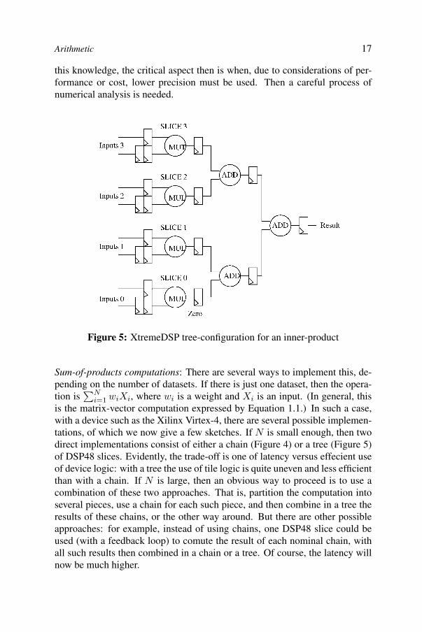
Figure 5: XtremeDSP tree-configuration for an inner-product

Sum-of-products computations: There are several ways to implement this, de-pending on the number of datasets. If there is just one dataset, then the opera-tion is

∑Ni=1 wiXi, where wi is a weight and Xi is an input. (In general, this

is the matrix-vector computation expressed by Equation 1.1.) In such a case,with a device such as the Xilinx Virtex-4, there are several possible implemen-tations, of which we now give a few sketches. If N is small enough, then twodirect implementations consist of either a chain (Figure 4) or a tree (Figure 5)of DSP48 slices. Evidently, the trade-off is one of latency versus effecient useof device logic: with a tree the use of tile logic is quite uneven and less efficientthan with a chain. If N is large, then an obvious way to proceed is to use acombination of these two approaches. That is, partition the computation intoseveral pieces, use a chain for each such piece, and then combine in a tree theresults of these chains, or the other way around. But there are other possibleapproaches: for example, instead of using chains, one DSP48 slice could beused (with a feedback loop) to comute the result of each nominal chain, withall such results then combined in a chain or a tree. Of course, the latency willnow be much higher.


With multiple datasets, any of the above approaches can be used, althoughsome are better than others — for example, tree structures are more amenableto pipelining. But there is now an additional issue: how to get data in andout at the appropriate rates. If the network is sufficiently large, then most ofthe inputs to the arithmetic units will be stored outside the device, and thenumber of device pins available for input/output becomes a minor issue. Inthis case, the organization of input/output is critical. So, in general, one needsto consider both large datasets as well as multiple data sets. The followingdiscussions cover both aspects.Storage and update of weights, input/output: For our purposes, Distributed-RAM is too small to hold most of the data that is to be processed, and therefore,in general Block-RAM will be used. Both weights and input values are storedin a single block and simualtaneously read out (as the RAM is dual-ported).Of course, for very small networks, it may be practical to use the Distributed-RAM, especially to store the weights; but we will in general assume networksof arbitrary size. (A more practical use for Distributed-RAM is the storage ofconstants used to implement activation functions.) Note that the disparity (dis-cussed below) between the rate of inner-product computations and activation-function computations means that there is more Distributed-RAM available forthis purpose than appears at first glance. For large networks, even the Block-RAM may not be sufficient, and data has to be periodically loaded into andretrieved from the FPGA device. Given pin-limitations, careful considerationmust be given to how this is done.

Let us suppose that we have multiple datasets and that each of these is verylarge. Then, the matrix-vector product of Equation 1.1, that is,

u = Wy

becomes a matrix-matrix product,

U = WY,

where each column of Y is associated with one input dataset. The mostcommon method used for matrix-matrix multiplication is the inner-productmethod; that is, each element of the output matrix is directly generated as aninner-product of two vectors of the input matrices. Once the basic method hasbeen selected, the data must be processed — in particular, for large datasets,this includes bringing data into, and retrieving data from, the FPGA — exactlyas indicated above. This is, of course, true for other methods as well.

Whether or not the inner-product method, which is a highly sequentialmethod, is satisfactory depends a great deal on the basic processor microar-chitecture, and there are at least two alternatives that should always be consid-

Arithmetic 19

ered: the outer-product and the middle-product methods.7 Consider a typical“naive” sequential implementation of matrix multiplication. The inner-productmethod would be encoded as three nested loops, the innermost of which com-putes the inner-product of a vector of one of the input matrices and a vector ofthe other input matrix:

for i:=1 to n dofor j:=1 to n do

for k:=1 to n doU[i,j]:=U[i,j]+W[i,k]*Y[k,j];

(where we assume that the elements of U [i, j] have all been initialized to zero.)Let us call this the ijk-method8, based on the ordering of the index-changes.The only parallelism here is in the multiplication of individual matrix elementand, to a much lesser extent (assuming the tree-method is used instead of thechain method) in the tree-summation of these products). That is, for n×n ma-trices, the required n2 inner-products are computed one at a time. The middle-product method is obtained by interchanging two of the loops so as to yieldthe jki-method. Now more parallelism is exposed, since n inner-products canbe computed concurrently; this is the middle-product method. And the outer-product method is the kij-method. Here all parallelism is now exposed: all n2

inner products can be computed concurrently. Nevertheless, it should be notedthat no one method may be categorically said to be better than another — it alldepends on the architecture, etc.

To put some meat to the bones above, let us consider a concrete example —the case of 2× 2 matrices. Further, let us assume that the multiply-accumulate(MAC) operations are carried out within the device but that all data has to bebrought into the device. Then the process with each of the three methods isshown in Table 1. (The horizontal lines delineate groups of actions that maytake place concurrently; that is within a column, actions separated by a linemust be performed sequentially.)

A somewhat rough way to compare the three methods is measure the ratio,M : I , of the number of MACs carried out per data value brought into thearray. This measure clearly ranks the three methods in the order one wouldexpect; also note that by this measure the kij-method is completely efficient(M : I = 1): every data value brought in is involved in a MAC. Nevertheless,it is not entirely satisfactory: for example, it shows that the kij-method to bebetter than the jki-method by factor, which is smaller that what our intuition

7The reader who is familiar with compiler technology will readily recognise these as vecorization (paral-lelization) by loop-interchange.8We have chosen this terminology to make it convenient to also include methods that have not yet been“named”.

Date post:	08-Mar-2018
Category:	Documents
Upload:	vankhanh
View:	221 times
Download:	0 times

FPGA IMPLEMENTATIONS OF NEURAL...

Documents