Fractal Boundaries of Complex Networks Jia Shao 1 , Sergey V. Buldyrev 2,1 , Reuven Cohen 3 , Maksim Kitsak 1 , Shlomo Havlin 4 , and H. Eugene Stanley 11 11 Center for Polymer Studies and Department of Physics, Boston University, Boston, Massachusetts 02215, USA 2 Department of Physics, Yeshiva University, 500 West 185th Street, New York, New York 10033, USA 3 Department of Mathematics, Bar-Ilan University, 52900 Ramat-Gan, Israel 4 Minerva Center and Department of Physics, Bar-Ilan University, 52900 Ramat-Gan, Israel (Dated: January 17, 2008sbckjhs.tex) We introduce the concept of the boundary of a complex network as the set of nodes at distance larger than the mean distance from a given node in the network. We study the statistical properties of the boundary nodes of complex networks. We find that for both Erd¨os-R´ enyi and scale-free model networks, as well as for several real networks, the boundary has fractal properties. In particular, the number of boundary nodes B follows a power-law probability density function which scales as B -2 . The size of the clusters, which are formed by the boundary nodes after removing the non-boundary nodes, also follows a power-law probability density function which scales as s -3 . These clusters are fractals with a fractal dimension d f ≈ 2. We present analytical and numerical evidence supporting these results for a broad class of networks. Many complex networks are “small world” due to the very small average distance d between two randomly cho- sen nodes. Usually d ∼ ln N , where N is the number of nodes [1–6]. Thus, starting from a randomly chosen node following the shortest path, one can reach any other node in a very small number of steps. This phenomenon is called “six degrees of separation” in social networks [4]. That is, for most pairs of randomly chosen people, the shortest “distance” between them is not more than six. Many random network models, such as Erd¨ os-R´ enyi network (ER) [1], Watts-Strogatz network (WS) [5] and random scale-free network (SF) [3, 7, 8], as well as many real networks, have been shown to possess this small- world property. Much attention has been devoted to the structural properties of networks within the average distance d from a given node. However, almost no attention has been given to nodes which are at distances greater than d from a given node. We define these nodes as the boundary nodes of the network. An interesting question is how many “friends of friends of friends etc...” one has at dis- tance greater than the average distance d? What is their probability distribution and what is the structure of the boundary? The boundary nodes have an important role in several cases, such as in the spread of viruses or infor- mation in a human social network. If the virus (informa- tion) spreads from one node to all its nearest neighbors, and from them to all next nearest neighbors and further on until the average distance, how many nodes do not get the virus (information), and what is their probability distribution? In this Letter, we find theoretically and numerically that the nodes at the boundary, which are of order N , exhibit similar fractal features for many types of net- works, including ER and SF models as well as several real networks. Song et al. [9] found that some networks have fractal properties while others do not. Here we show that almost all model and real networks including non-fractal networks have fractal features at their boundaries. Fig. 1 demonstrates our approach and analysis. For each node, we identify the nodes at distance ℓ from it as nodes in shell ℓ. We chose a random origin node and count the number of nodes B ℓ at shell ℓ. We see that B 1 =10, B 2 =11, B 3 =13, etc... We estimate the average distance d ≈ 2.9 by averaging the distances between all pairs of nodes. After removing nodes with ℓ<d =2.9, the network is fragmented into 12 clusters, with sizes s 3 ={1, 1, 2, 5, 1, 3, 1, 1, 8, 1, 2, 3}. FIG. 1: (Color on line) Illustration of shells and clusters orig- inating from a randomly chosen node, which is shown in the center (red). Its neighboring nodes are defined as shell 1, the nodes at distance ℓ are defined as shell ℓ. When removing all nodes with ℓ< 3, the remaining network becomes fragmented into 12 clusters. We begin our study by simulating ER and SF networks, and later present analytical proofs. Fig. 2a shows simu- lation results for the number of nodes B ℓ reached from a randomly chosen origin node for an ER network. The results shown are for a single network realization of size N = 10 6 , with average degree 〈k〉 = 6 and d ≈ 7.9 [10].
Transcript
Fractal Boundaries of Complex Networks
Jia Shao1, Sergey V. Buldyrev2,1, Reuven Cohen3,
Maksim Kitsak1, Shlomo Havlin4, and H. Eugene Stanley11
11Center for Polymer Studies and Department of Physics,
Boston University, Boston, Massachusetts 02215, USA2Department of Physics, Yeshiva University, 500 West 185th Street, New York, New York 10033, USA
3Department of Mathematics, Bar-Ilan University, 52900 Ramat-Gan, Israel4Minerva Center and Department of Physics, Bar-Ilan University, 52900 Ramat-Gan, Israel
(Dated: January 17, 2008sbckjhs.tex)
We introduce the concept of the boundary of a complex network as the set of nodes at distancelarger than the mean distance from a given node in the network. We study the statistical propertiesof the boundary nodes of complex networks. We find that for both Erdos-Renyi and scale-free modelnetworks, as well as for several real networks, the boundary has fractal properties. In particular, thenumber of boundary nodes B follows a power-law probability density function which scales as B−2.The size of the clusters, which are formed by the boundary nodes after removing the non-boundarynodes, also follows a power-law probability density function which scales as s−3. These clusters arefractals with a fractal dimension df ≈ 2. We present analytical and numerical evidence supportingthese results for a broad class of networks.
Many complex networks are “small world” due to thevery small average distance d between two randomly cho-sen nodes. Usually d ∼ lnN , where N is the numberof nodes [1–6]. Thus, starting from a randomly chosennode following the shortest path, one can reach any othernode in a very small number of steps. This phenomenonis called “six degrees of separation” in social networks[4]. That is, for most pairs of randomly chosen people,the shortest “distance” between them is not more thansix. Many random network models, such as Erdos-Renyinetwork (ER) [1], Watts-Strogatz network (WS) [5] andrandom scale-free network (SF) [3, 7, 8], as well as manyreal networks, have been shown to possess this small-world property.
Much attention has been devoted to the structuralproperties of networks within the average distance d froma given node. However, almost no attention has beengiven to nodes which are at distances greater than d froma given node. We define these nodes as the boundarynodes of the network. An interesting question is howmany “friends of friends of friends etc...” one has at dis-tance greater than the average distance d? What is theirprobability distribution and what is the structure of theboundary? The boundary nodes have an important rolein several cases, such as in the spread of viruses or infor-mation in a human social network. If the virus (informa-tion) spreads from one node to all its nearest neighbors,and from them to all next nearest neighbors and furtheron until the average distance, how many nodes do notget the virus (information), and what is their probabilitydistribution?
In this Letter, we find theoretically and numericallythat the nodes at the boundary, which are of order N ,exhibit similar fractal features for many types of net-works, including ER and SF models as well as several realnetworks. Song et al. [9] found that some networks havefractal properties while others do not. Here we show thatalmost all model and real networks including non-fractal
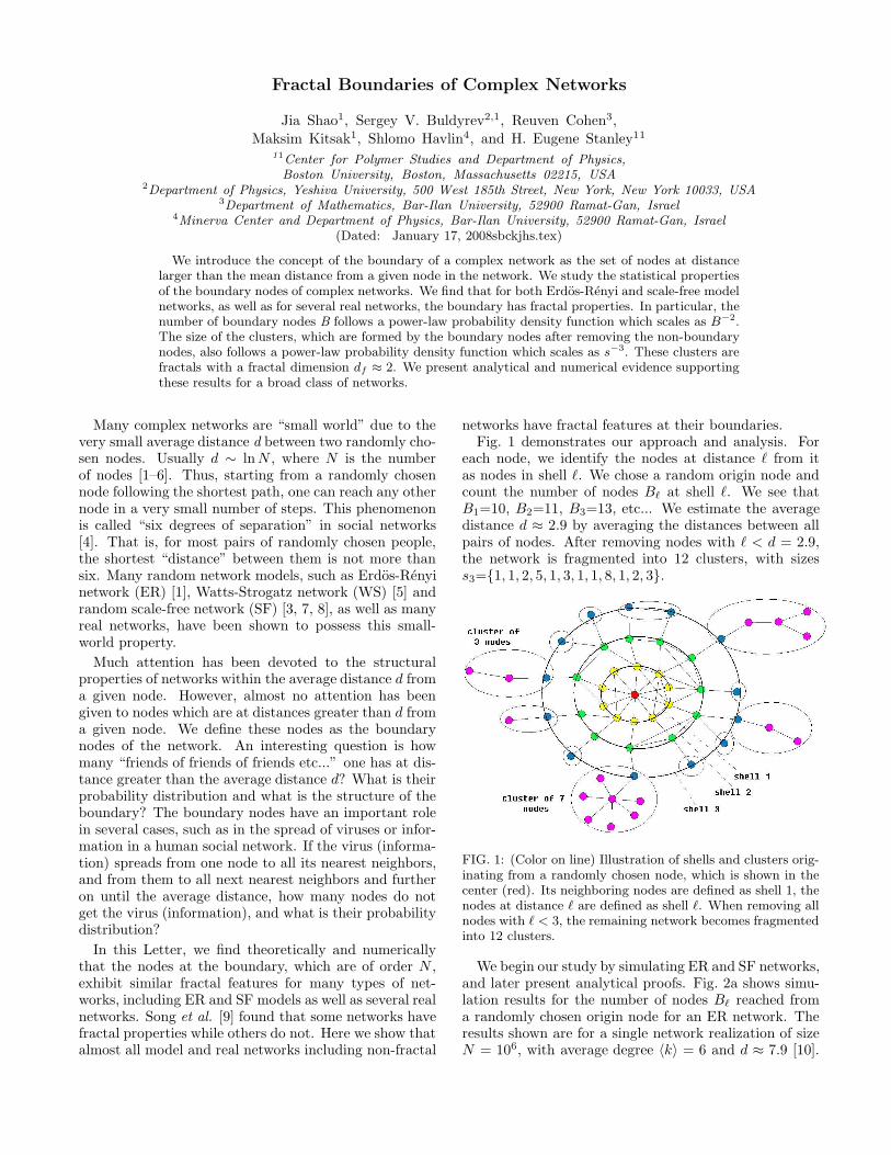
networks have fractal features at their boundaries.Fig. 1 demonstrates our approach and analysis. For
each node, we identify the nodes at distance ℓ from itas nodes in shell ℓ. We chose a random origin node andcount the number of nodes Bℓ at shell ℓ. We see thatB1=10, B2=11, B3=13, etc... We estimate the averagedistance d ≈ 2.9 by averaging the distances between allpairs of nodes. After removing nodes with ℓ < d = 2.9,the network is fragmented into 12 clusters, with sizess3={1, 1, 2, 5, 1, 3, 1, 1, 8, 1, 2, 3}.
FIG. 1: (Color on line) Illustration of shells and clusters orig-inating from a randomly chosen node, which is shown in thecenter (red). Its neighboring nodes are defined as shell 1, thenodes at distance ℓ are defined as shell ℓ. When removing allnodes with ℓ < 3, the remaining network becomes fragmentedinto 12 clusters.
We begin our study by simulating ER and SF networks,and later present analytical proofs. Fig. 2a shows simu-lation results for the number of nodes Bℓ reached froma randomly chosen origin node for an ER network. Theresults shown are for a single network realization of sizeN = 106, with average degree 〈k〉 = 6 and d ≈ 7.9 [10].
2
For ℓ < d, the cumulative distribution function P (Bl ),which is the probability that shell ℓ has more than Bℓ
nodes, decays exponentially for Bℓ > B∗ℓ , where B∗
ℓ isthe maximum typical size of shell ℓ [11]. However, forℓ > d, we observe a clear transition to a power law decay
behavior, where P (Bℓ) ∼ B−βℓ , with β ≈ 1 and the pdf
of Bℓ is P (Bℓ) ≡ dP (Bℓ)/dBℓ ∼ B−2ℓ . Thus, our results
suggest a broad “scale-free” distribution for the num-ber of nodes at distances larger than d. This power lawbehavior demonstrates the fractal nature of the bound-aries of network, suggesting that there is no characteristicsize and a broad range of sizes can appear in a shell atthe boundaries. Further fractal features of the boundarystructure will be shown below.
In SF networks, the degrees of the nodes, k, followa power law distribution function q(k) = ck−λ, wherec ≈ (λ − 1)kλ−1
m and km is the minimum degree of thenetwork, which we chose here to be 2. The largest degreeK is the natural upper cutoff, K ≈ kmN1/(λ−1) [12, 13].Fig. 2b shows, for SF networks with λ = 2.5, similar
power law results, P (Bℓ) ∼ B−βℓ for ℓ > d as for ER,
with a similar power β ≈ 1. We find similar results alsofor λ > 3 (not shown).
100
102
104
106
B10
-4
10-3
10-2
10-1
100
P(B
)
(a) ER
β=1.0
=11
=12
=13
l
l
l
l
l
100
102
104
106
B
10-4
10-3
10-2
10-1
100
P(B
)
(b) SF =9=10
=8=11
β=1.0
ll
l
l
l
l
100
101
102
103
104
B
10-3
10-2
10-1
100
P(B
)
β=1.0
(c) HEP
=9
=10l
l
l
l =11ll
=12l
100
101
102
103
104
B
10-3
10-2
10-1
100
P(B
) β=1.0
(d) AS
=6
=7
=4=5
l
l l l
l
l
FIG. 2: The cumulative distribution function, P (Bℓ), for tworandom network models: (a) ER network with N = 106 nodesand 〈k〉 = 6, and (b) SF network with N = 106 nodes andλ = 2.5, and two real networks: (c) the High Energy Parti-cle (HEP) physics citations network and (d) the AutonomousSystem (AS) Internet network. The shells with ℓ > d aremarked with their shell number. The thin lines from left toright represent shells ℓ =1, 2 ... respectively, with ℓ < d. Forℓ > d, P (Bℓ) follows a power-law distribution P (Bℓ) ∼ B−β
ℓ,
with β ≈ 1 (corresponding to P (Bℓ) ∼ B−2
ℓ for the pdf). Theappearance of a power law decay only happens for ℓ largerthan d ≈ 7.9 for ER and d ≈ 4.7 for the SF network. Thestraight lines represent a slope of −1.
To test how general is our finding, we also study severalreal networks (Figs. 2c, 2d), including the High EnergyParticle (HEP) physics citations network [14] and theAutonomous System (AS) Internet network [15, 16]. Our
results suggest that the fractal properties of the bound-aries appear also in both networks, with similar values ofβ ≈ 1 for ℓ > d [17].
-6 -4 -2 0 2 4 6 8l-(lnN/ln<k>)
10-5
10-4
10-3
10-2
10-1
100
<B
>/N
N=200N=400N=800N=8000N=32000N=128000N=10
6
(a) ER
l
1 2 3 4 5 6 7 8 9 10 11 12 13l
100
101
102
103
104
k +
ER N=128000 ER N=10
6
SF N=128000SF N=10
6
(b)
l1
~
100
102
104
106
B10
-8
10-6
10-4
10-2
100
PD
F
=1 =2 =3 =4 =5 =6 =7 =8
µ=1.5
(c) ER ( <d)l
lll
ll
l
ll
l
_
0 0.2 0.4 0.6 0.8 1x10
-3
10-2
10-1
100
x Eq. (6)
(d) ER
m=1
m=2
m=3
l
l+m
FIG. 3: (Color on line) (a) Normalized average number ofnodes at shell ℓ, 〈Bℓ〉/N as a function of ℓ−ln N/ ln〈k〉 for ERnetwork with < k >=6. For different N , the curves collapse.(b) kℓ + 1, which is 〈k2
ℓ 〉/〈kℓ〉, as function of ℓ shown for bothER and SF network. (c) The probability distribution function
P (Bℓ) in shells ℓ ≤ d for ER network. For small values of Bℓ,
P (Bℓ) ∼ Bµ
ℓ , where µ depends on the 〈k〉 of the network (Eq.(4)). (d) The fraction of nodes outside shell ℓ+m, xℓ+m, as afunction of xℓ for ER network, where xℓ is calculated for anypossible ℓ. The (red) lines represent the theoretical iterationfunction (Eq. (6)).
Next we ask how many nodes are on average at theboundaries? Are they a finite fraction of N , or less?In Fig. 3a, we study the mean number 〈Bℓ〉 in shell ℓ,and plot 〈Bℓ〉/N as function of ℓ − lnN/ ln〈k〉 for differ-ent values of N for ER network, where N denotes thesize of the giant component of the network. The termlnN/ ln〈k〉 represents the average distance d of the net-work [2]. We find that, for different values of N , thecurves collapse, supporting a relation independent of net-work size N . Since 〈Bℓ〉/N is apparently constant andindependent of N , it follows that 〈Bℓ〉 ∼ N , i.e., a finitefraction of N nodes appear at each shell including shellswith ℓ > d. We find similar behavior for SF networkwith λ = 3.5 (not shown). The branching factor [12]
of the network is k = 〈k2〉/〈k〉 − 1, where the averagesare calculated for the entire network. Similarly, we definekℓ = 〈k2
ℓ 〉/〈kℓ〉−1, where the averages are calculated only
for nodes in shell ℓ. Above the average distance, kℓ + 1decreases with ℓ for both ER and SF networks (Fig. 3b).Thus, at the shells where power law behavior of P (Bℓ)
appears (Fig. 2), the nodes have much lower kℓ + 1 com-
pared with the entire network. The approach of kℓ +1 to1 (ER network) and 2 (SF network) is consistent with acritical behavior at the boundaries of the network [12].
Fig. 3c shows that P (Bℓ) for ℓ < d and small values of
3
Bℓ increase as a power law, P (Bℓ) ∼ Bµℓ for ER network,
where µ depends on k (supporting the theory developedbelow). We define the fraction of nodes outside shell mas xm = 1 − (
∑mℓ=1 Bℓ)/N . There exists a functional
relation which is independent of ℓ between any two xℓ
and xℓ+m (m = 1, 2, 3...), for ER network in Fig. 3d.Figs. 3c, 3d provide empirical evidences for the theorydeveloped below.
100
102
104
106
s
100
102
104
106
108
n(s
)
=5 =6 =7
(a) SF
θ=3.0
l
ll
l
l10
010
110
210
310
4
s10
0
102
104
106
108
n(s
) =5 =7 =9θ=3.0
(b) HEP
lll
l
l
100
101
102
d 10
0
102
104
106
108
s
=6 =6.5 =7
ϕ=1.9
lll
(c) SF
l
l
1 10d
100
102
104
106
s
=5 =6 =7 =8
ϕ=2.0
(d) HEP
llll
l
l
FIG. 4: The number of clusters of sizes sℓ, n(sℓ), as functionof sℓ after removing nodes within shell ℓ for: (a) SF networkwith N = 106 and λ = 2.5, (b) HEP citations network, andsℓ as function of average distance dℓ of the clusters for (c) SFnetwork with N=106 and λ = 2.5, (d) HEP citations network.The relation between n(sℓ) and sℓ is characterized by a powerlaw, n(sℓ) ∼ s−θ
ℓ , with θ ≈ 3. Also, sℓ is power law with dℓ,sℓ ∼ dϕ
ℓ , with ϕ ≈ 2.
Next, we study the structural properties of the bound-ary. Removing all nodes that are within a distance ℓ > d(not including shell ℓ), the network will become frag-mented into several clusters (see Fig. 1). We denote thesize of those clusters as sℓ, the number of clusters of sizesℓ as n(sl), and the average distance in the clusters as dℓ
[21]. We find n(s) ∼ s−θ, with θ ≈ 3.0 (Figs. 4a and 4b).Similar relations are also found for ER and other realnetworks. The relation between the size of the clusterssℓ and their mean distance dℓ is shown in Figs. 4c and 4d,for SF (λ = 2.5) and HEP citations networks respectively.These plots suggest a power law relation, sℓ ∼ dϕ
ℓ , withϕ ≈ 2. It indicates that the clusters at the boundariesare fractals with fractal dimension df = 2 as percula-tion clusters at criticality [22]. Note that, for very largeclusters their average distances dℓ decrease with size, sug-gesting that the largest clusters are not fractals. We findthat the fractal dimension is df = ϕ ≈ 2 also for ER, SFwith λ = 3.5 and some real networks.
Next we present analytical derivations supporting theabove numerical results. We denote the degree distri-bution of a network as q(k). The probability of reach-ing a node with k outgoing links through a link is
q(k) = (k + 1)q(k + 1)/〈k〉. We define the generatingfunction of q(k) as G0(x) ≡
∑∞k=0 q(k)xk, the generating
function of q(k) as G1(x) =∑∞
k=0 q(k)xk = G′
0(x)/〈k〉.
For ER networks we have G0(x) = G1(x) = e〈k〉(x−1).The generating function for the number of nodes, Bm, atthe shell m is [23]:
Gm(x) = G0(G1(...(G1(x)))) = G0(Gm−11 (x)), (1)
where G1(G1(...)) ≡ Gm−11 (x) is the result of applying
G1(x), m − 1 times. P (Bm), which is the pdf of Bm, is
the coefficient of xBm in the Taylor expansion of Gm(x).For shells with large m but still much smaller than d,
we expect [23] that the number of nodes will increase by a
factor of k. Hence, we conclude that Gm−11 (x) converges
to a function of the form f((1−x)km) for large m (m <<d), and f(x) satisfies the functional relation:
G1(f(y)) = f(yk), (2)
where y = 1 − x.The solution of G1(f∞) = f∞ gives the probability
that a link is not connected to the giant component of thenetwork [24]. We can assume an asymptotic functionalform, f(y) = f∞ + ay−δ + 0(yδ). Expanding both sidesof Eq. (2) we obtain:
G1(f∞) + G′
1(f∞)ay−δ = f∞ + ak−δy−δ + 0(yδ). (3)
Since G1(f∞) = f∞, we have δ = − lnG′1(f∞)/ ln k.
If q(1) = 0 and q(2) 6= 0, from G1(f∞) = f∞, we have
f∞ = 0 and G′
1(f∞) = 2q(2)/〈k〉. If q(2) = q(1) = 0,then δ = ∞, which indicates that f(y) has an exponentialsingularity. Therefore, networks with minimum degreekm ≥ 3 do not exhibit the following properties for m <<d, and therefore have no fractal boundaries.
Applying the Tauberian theorem [25] to f(y), whichhas a power law singularity, we conclude that the Taylorexpansion coefficient of Gm(x) = G0(f((1 − x)km−1)),P (Bm), behaves as Bµ
m with an exponential cutoff at
B∗m ∼ km. When q(1) 6= 0 and q(2) 6= 0, we have
µ = δ − 1 and when q(1) = 0 and q(2) 6= 0, we haveµ = 2δ−1. Thus the distribution of the number of nodesin the shell m with m << d has a power law tail for smallvalues of Bm:
P (Bm) ∼ Bµm. (4)
For ER network, Eq. (4) is supported by simulationsfor m ≤ d in Fig. 3c.
The above considerations are correct only for m < d,for which the depletion of nodes with large degree in thenetwork is insignificant.
In the network, the shells behave almost deterministi-cally and there exists a functional relation between anytwo shell m and shell n with n > m (a detailed proof willbe given elsewhere):
xn = G0(Gn−m1 (G−1
0 (xm))), (5)
4
where xm = 1 − (∑m
ℓ=1 Bℓ)/N is the fraction of nodesoutside shell m.
For ER networks, Eq. (5) yields:
xℓ+1 = e〈k〉(xℓ−1) = Σ∞ℓ=0q(k)xk
ℓ , (6)
which is valid for all possible ℓ. We test it in Fig. 3d.When m << d and n >> d, using the same consider-
ations as before it can be shown that:
xn = [ak(1 − xm)]−µ−1 + x∞, (7)
where x∞ = G0(f∞) = f∞, a is a constant.Based on Eqs. (4) and (6), expressing xm and xn in
terms of Bm and Bn, we find that for m << d andn >> d, Bn ∼ B−µ−1
m . Using P (Bn)dBn = P (Bm)dBm,
we obtain P (Bn) ∼ B−1−µ/(µ+1)−1/(µ+1)n = B−2
n , sup-porting the numerical findings in Fig. 2.
These results are rigorous when k exists and when theminimum degree km ≤ 2. For SF networks with λ < 3,k diverges for N → ∞. But for finite N , k still exists.Thus the above results can also be applied to the case ofλ < 3. For both ER and SF networks with km ≥ 3, thepower law of P (Bn) with n >> d cannot be observed, aswe indeed confirm by simulations.
The cluster size distribution in percolation at someconcentration p close to pc is determined using the for-
mula [12]:
Pp(s > S) ∼ S−τ+1 exp(−S|p − pc|−1/σ) . (8)
In the case of random networks the percolation thresholdis given by pc = 1/k. In the exterior of the shell n (n >>
d), we can estimate |p−pc| ∼ (k(xn)−1)/k, where k(xn)is calculated from nodes in the exterior of the shell n.
The cluster size distribution can be estimated by con-sidering introducing a sharp exponential cutoff at s =S∗
n ∼ |k(xn) − 1|−1
σ , so that Pn(s > S) ∼ S−τ+1P (S∗n >
S), where P (S∗n > S) is the probability for a given shell
to have S∗n > S.
Since xn − x∞ has a smooth power law distributionand k(x∞) < 1, |k(xn) − 1| < S−σ = ε, it is propor-tional to ε. Thus P (S∗
n > S) ∼ S−σ and Pn(s > S) =S−τ+1−σ. Therefore the cluster size distribution followsn(s) ∼ s−(τ+σ).
For ER networks and SF networks with λ > 4, τ = 2.5and σ = 0.5, the above derivations lead to n(s) ∼ s−3.For SF networks with 2 < λ < 4, τ = (2λ−3)/(λ−2) andσ = |λ − 3|/(λ − 2) [22]. Thus, for λ > 3, there will bens ∼ s−3 for SF networks. We conjecture ns ∼ s−3 evenfor 2 < λ < 3, although in this case k(xn) does not existand the above derivations are not valid. Our numericalsimulations support these results in Fig. 4a, b.
[1] P. Erdos and A. Renyi, Publ. Math. 6, 290 (1959); Publ.Math. Inst. Hung. Acad. Sci. 5, 17 (1960).
[2] B. Bollobas, Random Graphs (Academic, London, 1985).[3] R. Albert and A.-L.Barabasi, Rev. Mod. Phys. 74,
47(2002).[4] S. Milgram, Psychol. Today 2, 60-67 (1967).[5] D. J. Watts and S. H. Strogatz, Nature (London) 393,
440 (1998).[6] R. Cohen and S. Havlin, Phys. Rev. Lett. 90, 058701
(2003).[7] S. N. Dorogovtsev and J. F. F. Mendes, Evolution of Net-
works: from Biological nets to the Internet and WWW
(Oxford University Press, New York, 2003).[8] R. Pastor-Satorras and A. Vespignani, Evolution and
Structure of the Internet: a statistical physics approach
(Cambridge University Press, 2004).[9] C. Song et al., Nature (London) 433, 392 (2005); Nature
Physics 2, 275 (2006).[10] Different realizations yield similar results. In one realiza-
tion, a certain fraction of nodes are randomly taken tobe origin. The histogram is obtained from Bℓ belongingto different origin nodes.
[11] The behavior of the pdf of Bℓ for ℓ < d will be discussedlater and is shown in Fig. 3c.
[12] R. Cohen et al., Phys. Rev. Lett. 85, 4626 (2000).[13] S. N. Dorogovtsev and J. F. F. Mendes, Phys. Rev. E 63,
062101 (2001).[14] Derived from the HEP section of arxiv.org;
http : //vlado.fmf.uni−lj.si/pub/networks/data/hep−th/hep − th.htm (website of Pajek).
[15] Y. Shavitt and E. Shir, DIMES - Let-ting the Internet Measure Itself, http ://www.arxiv.org/abs/cs.NI/0506099
[16] S. Carmi et al., PNAS 104, 11150 (2007).[17] We also find similar results (not shown here) for protein
interaction yeast network [18, 19] and for the E.coli cel-lular network [18, 20].
[18] http : //www.nd.edu/ alb/ (homepage of A.L.Barabasi).[19] H. Jeong et al., Nature (London) 411, 41 (2001).[20] H. Jeong et al., Nature (London) 407, 651 (2000).[21] Fractional shells with ℓ + a (0 < a < 1) are used here by
removing nodes within shell ℓ and a fraction a of nodesat shell ℓ.
[22] R. Cohen et al., Phys. Rev. E 66, 036113 (2002); Chap.4 in Handbook of graphs and networks, Eds. S. Bornholdtand H. G. Schuster (Wiley-VCH, 2002)
[23] M. E. J. Newman et al., Phys. Rev. E 64, 026118 (2001).[24] L. A. Braunstein et al., Int. J. Bifurcation and Chaos 17,
2215 (2007).[25] Weiss, G. H. Aspects and Applications of the Random