Fraction of natural area as main predictor of net CO2

emissions from cities

Annika Nordbo1, Leena Järvi

1, Sami Haapanala

1, Curtis R. Wood

2, Timo Vesala

1

1University of Helsinki, Department of Physics

2Finnish Meteorological Institute

annika.nordbo -ÅT- helsinki.fi

leena.jarvi -ÅT- helsinki.fi

sami.haapanala -ÅT- helsinki.fi

curtis.wood -ÅT- fmi.fi

timo.vesala -ÅT- helsinki.fi

An edited version of this paper was published by AGU. Copyright 2012 American

Geophysical Union.

Nordbo, A., L. Järvi, S. Haapanala, C. R. Wood, and T. Vesala (2012), Fraction of

natural area as main predictor of net CO2 emissions from cities, Geophys. Res. Lett.,

39, L20802, doi:10.1029/2012GL053087. To view the published open abstract, go to

http://dx.doi.org and enter the DOI.

Abstract

Cities account for most anthropogenic greenhouse-gas emissions, CO2 being most important.

We evaluate the net urban contribution to CO2 emissions by performing a meta-analysis of all

available 14 annual CO2 budget studies. The studies are based on direct flux measurements

using the eddy-covariance technique which excludes all strong point sources. We show that

the fraction of natural area is the strongest predictor of urban CO2 budgets, and this fraction

can be used as a robust proxy for net urban CO2 emissions. Up-scaling, based on that proxy

and satellite mapping of the fraction of natural area, identifies urban hotspots of CO2

emissions; and extraction of 56 individual cities corroborates their inventory-based estimates.

Furthermore, cities are estimated as carbon-neutral when the natural fraction is about 80%.

This fresh view on the importance of cities in climate change treats cities as urban

ecosystems: incorporating natural areas like vegetation.

Main text

1. Introduction

Over 70% of global energy-related CO2 emissions originate from cities [WEO, 2008;

Rosenzweig et al., 2010], and fossil fuel combustion―in transportation, industry, and

housing―is the dominant urban CO2 source. Besides CO2 sources, cities typically have green

areas that are carbon sinks through photosynthetic uptake. Since over half of global

population is city-based (UN, http://esa.un.org/unpd/wup), urban areas are hotspots of

greenhouse gas (GHG) emissions and the focus of innovation in climate-change mitigation

[Kennedy et al., 2009]. International negotiations are a key part of climate-change mitigation

via GHG-emission reductions. These negotiations necessitate quantification of net GHG

exchange between surface and atmosphere, especially CO2. The eddy-covariance method, the

only direct way of measuring surface–atmosphere GHG exchange, is widely applied in

natural surroundings. Extensive measurement networks have emerged (AmeriFlux

[Baldocchi et al., 2001], EuroFlux [Valentini et al., 2000], AsiaFlux [Mizoguchi et al.,

2009]), and continental-scale budgets have recently been estimated of biological GHG fluxes

for Europe [Schulze et al., 2009] and global terrestrial ecosystem CO2 uptake [Beer et al.,

2010]. Measurements in urban environments have only, during the past year, become

extensive enough to enable synthesis of CO2 exchange at numerous eddy-covariance sites

(Grimmond and Christen, 2012). Individual local-scale and city-scale budget estimates

include both direct emissions from the city and contributions from vegetation: photosynthetic

uptake and respirative emissions, which are seldom within inventories. We thus denote

estimates from direct flux measurements as net urban ecosystem exchange (NUE); a

counterpart to net ecosystem exchange, used canonically for non-urban fluxes. NUE

describes the CO2 budget of urban ‘background activity’: including direct emissions from e.g.

buildings and traffic; but excluding strong point sources like power stations. This is not

disadvantageous, since emissions from such strong point sources are well-described in

inventories (Carbon Monitoring and Action, http://carma.org), whereas NUE has remained

unresolved until now.

Apart from direct flux measurements, multiple studies have gathered inventories of

annual GHG emissions from nations [Hertwich and Peters, 2009] or individual urban areas [

Dodman, 2009; Kennedy et al., 2011] based on consumption statistics. Furthermore, area-

specific inventories of CO2 emissions have been utilized for mapping global emissions based

on population densities and night-time lights [Raupach et al., 2010; Oda and Maksyutov,

2011], and CO2 emissions in USA have been down-scaled to a 10 km grid scale [Gurney et

al., 2009; Parshall et al., 2010]. These inventory-based methods, as indirect estimations of

GHG emissions, have inherent disadvantages: fossil fuels are often not consumed where

purchased, population data represent commuting inconsistently, and there is no clear

literature consensus whether emissions estimates should be end-use or only from those

emissions produced within city borders. Conversely, the definition of NUE is rigorous: it is

an in-situ measure of the local CO2 budget, excluding any city-related emissions located

outside city borders (e.g. aviation, marine, electricity production, product manufacturing).

We present a meta-analysis of a compilation of 17 annual NUE budgets from direct

flux measurements from 14 urban eddy-covariance towers, and analyze the predictors of

surface–atmosphere exchange. The fraction of natural area in a city (derived from satellite

data) is used as a proxy for estimating regional variation of NUE in parts of North America,

Europe, and eastern Asia; and those estimates for particular cities are compared against

inventory-based estimates. Here natural fraction means the fraction of land area that is

covered by surface types existing in nature (e.g. grass, trees, soil, sand), whereas urban

fraction means all non-vegetative, human-constructed elements. Additionally, a natural

fraction is conjectured for a carbon-neutral city (annual NUE zero).

2. Data and methods

The eddy-covariance technique is tower-based and the measurements’ source area is several

hectares: depending on the upwind surface, measurement height, and flow properties [Vesala

et al., 2008]. The technique is based on measuring simultaneous turbulent variations in wind

and gas concentrations (e.g. CO2): output typically being 30-minute fluxes. The

measurements used in this study (Auxiliary Figure 1, Auxiliary Table 1) represent over

16 000 days’ measurements with 58% data coverage (the percentage is typical for the

method). Data were processed by original authors with widely-accepted procedures,

including quality-screening, the main cause of data-loss. Time series consequently were gap-

filled (typical errors are below 5% [Järvi et al., 2012]) to enable annual-sum calculations.

Furthermore, typical random errors are under 20% for half-an-hour fluxes [Aubinet et al.,

2012; Nordbo et al., 2012], and the random error is assumed negligible for annual sums of

NUE. Data coverage at each site is taken into account when analyzing predictors of NUE and

non-linear least-squares optimization is used for non-linear fits.

The natural fraction (fn) is estimated from the urban fraction (fu = 1– fn) which can be

retrieved from global satellite data. The urban fraction is derived from binary (urban/non-

urban), 500-meter-resolution data from the MODIS satellite in 2001–2002 [Schneider et al.,

2009, 2010]. Urban area was defined as “a place dominated by built environment”—which

includes all non-vegetative, human-constructed elements like buildings, roads, and runways.

The mean accuracy of the binary data exceeds 93% [Schneider et al., 2009]. Binary data were

converted by us to fu by aggregating to 4x4 km resolution, each aggregated pixel based on 64

binary values. GHG inventories from 56 urban areas (cities, metropolitan areas, counties) in

North America, Europe, and eastern Asia were compiled (Auxiliary Table 2). Corresponding

NUE estimates are subsequently retrieved using the 4 km resolution values of fu within

official administrative areas (Database of Global Administrative Areas, www.gadm.org). A

pixel is included if the pixel’s center is within the administrative area. If beyond 50% of a

pixel is water, the pixel is omitted. If administrative areas are below 1000 km2, fu data are

disaggregated back to 500-meter resolution to minimize edge problems.

3. Results and Discussion

3.1 Predictors of net urban ecosystem exchange

The compilation of direct annual NUE measurements shows that urban areas are sources of

CO2 (Figure 1). Annual emissions are as high as 9.7 kg C m–2

yr–1

in London [Helfter et al.,

2011], which is forty times the typical uptake of grassland [Soussana et al., 2007] and over

ten times the global median terrestrial ecosystem uptake [Beer et al., 2010]. The Minnesota

site, conversely, is only a very small CO2 source, since the measurements were carried out in

an urban park [Hiller et al., 2011].

The fraction of natural area (fn) in the source area of the measurements is a robust proxy

for annual NUE (coefficient of determination r2 = 0.84, Figure 1), especially when

considering the variety between cities’ surface cover and latitude. Previously, non-gapfilled

CO2 fluxes (mostly) from summertime have been compared with vegetation fraction for 18

sites [Velasco and Roth, 2010] and with building fraction for 22 sites [Grimmond and

Christen, 2012]. Five annual CO2 budgets were compared as a function of vegetation fraction

[Helfter et al., 2011], but two of the budgets were based on measurements during one season,

and the given exponential fit saturated to an unrealistic value for complete vegetation cover

(2.5 kg C m-2

yr-1

). Population density has a lesser correlation with NUE (r2 = 0.60, rms 1.13

kg C m-2

yr-1

Auxiliary Figure 3), although population density is an indicator for energy

consumption, perhaps because traffic-fuel demand decreases as population density grows

[Kennedy et al., 2009; Karathodorou et al., 2010]. A correlation between annual CO2 budgets

and population density has not been seen before [Helfter et al., 2011].

The strong relationship between NUE and fn can be explained by the indirect links that

fn has to many factors determining CO2 release: greater fn is consistent with a lesser road and

population density, which thus limits CO2 release from fossil-fuel combustion and human

respiration [Moriwaki and Kanda, 2004]. Greater fn can also reduce pedestrian and building

cooling-needs, e.g. via shading effects of trees [Simpson, 2002]. Vegetation itself is also a

key NUE component through daytime sequestration of carbon via photosynthesis. The non-

linearity of the relationship in Figure 1 comes from the dependency of population density on

urban density: population grows exponentially when a dense city becomes even more

compact [Pozzi and Small, 2005] since cities do not only grow horizontally but also

vertically. Furthermore, dense urban living may generate less per-capita GHG emissions

compared to rural living, given a similar income level, since urban areas often have lower

emissions than the national average [ Brown et al., 2009; Dodman, 2009] or rural areas

[Parshall et al., 2010]. Standard of living is a predictor for CO2 release, since greater

incomes often lead to greater consumption [Kennedy et al., 2009]. Conversely, technological

advances—usually a consequence of wealth increase—can decrease the emission intensity of

CO2 per unit GDP: the overall global emission intensity has decreased by 41% from 1971 to

2007 [International Energy Agency, 2009].

A minimum fn requirement for a carbon-neutral city (annual NUE zero) can be

interpreted from the fit in Figure 1: cities are net sinks of CO2 if their natural fraction exceeds

about 80%. This value can be used as a first rule-of-thumb estimate in urban planning, among

other indicators [Kennedy et al., 2011]. The general definition of a carbon-neutral city suffers

from a scoping problem: some definitions require zero carbon emissions, others allow

emissions to be balanced by sequestration or export of low-carbon goods [Kennedy and

Sgouridis, 2011]. In our case, the limit for carbon-neutrality treats the city as an urban

ecosystem comprising in-situ sinks and sources of CO2 within the city boundaries. Increasing

the natural land area fraction within a city is expected to decrease the CO2 emissions per unit

area, but this is not a general solution for climate-change mitigation: if natural area

substitutes previously-occupied buildings, the per-capita emissions might increase, if the

living density decreases. Conversely, if an unused urban area (e.g. abandoned car park) is

transformed into a vegetated area, then there is an obvious, but small, net gain. Green roofs,

to the contrary, are usually a net gain in energy savings [Sailor et al., 2012] and

photosynthetic uptake of CO2.

3.2 Regional estimates for NUE

The strength of fn as a predictor of NUE provides a means for producing annual NUE

estimates based solely on land-cover data, using the relationship in Figure 1. The global fu is

calculated based on satellite observations for North America, Europe, and eastern Asia

(Section 2). These areas were chosen for mapping since all-but-one of the flux sites are

within these regions and thus the relationship in Figure 1 is assumed to be applicable within

these regions. In Europe, high urbanization dominates around the Benelux countries,

Germany, and southern England (Figure 2 a). In North America, the north-east coast of USA,

the Great Lakes region, Los Angeles, and Florida have conspicuously continuous and high

urban fraction (Auxiliary Figure 4a). In eastern Asia, the east coast of China and the Tokyo

metropolis have prominently-high urban fractions (Auxiliary Figure 5a).

Mid-Europe and United Kingdom are regions of high NUE in Europe (Figure 2 b). The

summed NUE over EU25 and EU27 (EU countries prior to and after 2007) are 410 Tg C yr–1

and 414 Tg C yr–1

, from which about 9% can be allocated to human respiration of the whole

population. The inventory-based emissions were twice the NUE (767 Tg C yr–1

in 2006)

[WEO, 2008], and NUE is almost four times the uptake of CO2 by biological fluxes (–102 ±

23 Tg C yr–1

, EU25) [Schulze et al., 2009]. The inventory-based emissions and NUE are not

intended to coincide, since some inventories include both strong point sources and emissions

occurring outside the city borders. Furthermore, NUE includes vegetation uptake, whereas

the inventories only include CO2 emissions and might include emissions of other GHGs.

In North America, the regional distribution of NUE follows that of urban fraction

(Auxiliary Figure 4b). The summed NUE is 460 Tg C yr–1

for USA48 (i.e. all states excluding

Alaska and Hawaii). From this, 5% can be allocated to human respiration of the whole

population (76.3 kg C yr–1

per person [Moriwaki and Kanda, 2004]) and about 5% to uptake

by urban trees (23 Tg C yr–1

) [Nowak and Crane, 2002]. In 2006, the inventory-based CO2

emissions from urban areas in USA were three times the NUE (1228 Tg C yr–1

) [WEO,

2008].

In eastern Asia, a large area of NUE sink is seen in north-east China where low urban

fraction is observed (Auxiliary Figure 5b). Chinese urbanization is characterized by a

continuous sprawl as an opposite to the more confined city structures seen in Europe (see also

Auxiliary Figure 2). To the contrary, the metropolitan areas of Tokyo, Seoul, Beijing, and

Shanghai arise as large CO2 sources. The NUE of Japan is 77 Tg C yr–1

, which is 22% of the

country-wide inventory estimate [Nojiri et al., 2012]. An estimate for the whole of China is

not given, since the sites in Figure 1 are not representative of China as a whole.

3.3 NUE and inventories of individual cities

The NUE estimates of urban areas are expected to relate to inventories, though they are also

expected to be systematically lower (as discussed above). Following this reasoning, a set of

56 GHG inventories from individual cities, or metropolitan areas, was collected in order to

conduct an independent comparison against the corresponding NUE estimates (see Auxiliary

Table 2). The NUE estimates are lower than the inventory-based GHG emissions for all cases

but Prague (slope 0.50, Figure 3 ). The inclusion of strong point sources in inventories can be

seen for example for Rotterdam where over 60% of emissions are due to energy industries.

Nevertheless, there is a clear linear dependency (r2 = 0.72, rms = 1.42 kg C m

–2 yr

–1), and 22

out of the 56 cities are net CO2 sinks. This result corroborates the usability of the proxy of

NUE as a function of fn, and confirms its use as a robust independent check against

international inventory studies.

4. Summary and Conclusions

The urban CO2 budgets (Figure 2, Auxiliary Figures 4 and 5) are the first continental-scale

estimations from direct flux measurements. The mapping estimation treats cities as

ecosystems, i.e. incorporating vegetation. The mapping is solely from the relationship

between the CO2 budget and the natural land fraction; the 14 eddy-covariance stations are

assumed representative at continental scale—resulting in high uncertainties in estimates of

annual CO2 budgets. Direct validation of the continental-scale NUE parameterization is not

possible due to the non-existence of another method that could provide CO2 budgets of urban

ecosystems. Nevertheless, the high correspondence of our continental-scale estimates with

individual cities’ inventory-based estimates (Figure 3) supports the new method’s robustness.

The inventory-based estimates exceed the parameterized NUE (median ratio 1.33), this is

reasonable since NUE lacks strong point sources and includes vegetative uptake.

Direct urban-flux measurements have become comprehensive enough to benefit

decision-makers and urban planners. Additional urban CO2 budget measurements, extending

beyond a year, are needed to represent diverse urban morphologies (very high or low fu) and

climates (Asia, Africa, and South America). Until present only short-term urban CH4 [Gioli et

al., 2012] and N2O [Famulari et al., 2010] campaigns have been under-taken, although their

anthropogenic emissions are increasing [Montzka et al., 2012]; the need for long-term flux

measurements is clear.

Acknowledgements

For funding we thank the Academy of Finland Centre of Excellence program (project no

1118615), the Academy of Finland project 138328, the Academy of Finland ICOS project

(263149), the EU ICOS project (211574), the EU GHG-Europe project (244122) and an EU

FP7 grant (ERC 227915). For the satellite surface-cover data we thank Annemarie Schneider.

We acknowledge Hotel Torni for providing a platform for eddy-covariance measurements.

Reference list

Aubinet, M., T. Vesala, and D. Papale (Eds.) (2012), Eddy Covariance - A Practical Guide to

Measurement and Data Analysis, Springer atmospheric sciences, the Netherlands.

Baldocchi, D. et al. (2001), FLUXNET: A new tool to study the temporal and spatial

variability of ecosystem-scale carbon dioxide, water vapor, and energy flux densities, Bull.

Am. Meteorol. Soc., 82, 2415-2434.

Beer, C. et al. (2010), Terrestrial Gross Carbon Dioxide Uptake: Global Distribution and

Covariation with Climate, Science, 329, 834-838.

Bergeron, O. and I. B. Strachan (2011), CO2 sources and sinks in urban and suburban areas

of a northern mid-latitude city, Atmos. Environ., 45, 1564-1573.

Brown, M. A., F. Southworth, and A. Sarzynski (2009), The geography of metropolitan

carbon footprints, Policy and Society, 27, 285-304.

Christen, A., N. C. Coops, B. R. Crawford, R. Kellett, K. N. Liss, I. Olchovski, T. R. Tooke,

M. van der Laan, and J. A. Voogt (2011), Validation of modeled carbon-dioxide emissions

from an urban neighborhood with direct eddy-covariance measurements, Atmos. Environ., 45,

6057-6069.

Coutts, A. M., J. Beringer, and N. J. Tapper (2007), Characteristics influencing the variability

of urban CO2 fluxes in Melbourne, Australia, Atmos. Environ., 41, 51-62.

Crawford, B., C. S. B. Grimmond, and A. Christen (2011), Five years of carbon dioxide

fluxes measurements in a highly vegetated suburban area, Atmos. Environ., 45, 896-905.

Dodman, D. (2009), Blaming cities for climate change? An analysis of urban greenhouse gas

emissions inventories, Environ. Urban., 21, 185-201.

Famulari, D., E. Nemitz, C. Di Marco, G. J. Phillips, R. Thomas, E. House, and D. Fowler

(2010), Eddy-covariance measurements of nitrous oxide fluxes above a city, Agric. For.

Meteorol., 150, 786-793.

Gioli, B., P. Toscano, E. Lugato, A. Matese, F. Miglietta, A. Zaldei, and F. P. Vaccari (2012),

Methane and carbon dioxide fluxes and source partitioning in urban areas: The case study of

Florence, Italy, Environ. Pollut., 164, 125-131.

Grimmond, C. S. B. and A. Christen (2012), Flux measurements in urban ecosystems,

Fluxletter - The newsletter of FLUXNET, 5, 1-8.

Gurney, K. R., D. L. Mendoza, Y. Zhou, M. L. Fischer, C. C. Miller, S. Geethakumar, and

Du Can,Stephane De La Rue (2009), High Resolution Fossil Fuel Combustion CO2 Emission

Fluxes for the United States, Environ. Sci. Technol., 43, 5535-5541.

Helfter, C., D. Famulari, G. J. Phillips, J. F. Barlow, C. R. Wood, C. S. B. Grimmond, and E.

Nemitz (2011), Controls of carbon dioxide concentrations and fluxes above central London,

Atmos. Chem. Phys., 11, 1913-1928.

Hertwich, E. G. and G. P. Peters (2009), Carbon Footprint of Nations: A Global, Trade-

Linked Analysis, Environ. Sci. Technol., 43, 6414-6420.

Hiller, R. V., J. P. McFadden, and N. Kljun (2011), Interpreting CO2 Fluxes Over a Suburban

Lawn: The Influence of Traffic Emissions, Bound. -Layer Meteorol., 138, 215-230.

International Energy Agency (2009), CO2 emissions from fuel combustion, IEA Statistics, 1-

115.

Järvi, L., A. Nordbo, H. Junninen, A. Riikonen, J. Moilanen, E. Nikinmaa, and T. Vesala

(2012), Seasonal and annual variation of carbon dioxide surface fluxes in Helsinki, Finland,

in 2006-2010, Atmos. Chem. Phys. Discuss., 12, 8355-8396.

Karathodorou, N., D. J. Graham, and R. B. Noland (2010), Estimating the effect of urban

density on fuel demand, Energy Econ., 32, 86-92.

Kennedy, C., S. Pincetl, and P. Bunje (2011), The study of urban metabolism and its

applications to urban planning and design, Environ. Pollut., 159, 1965-1973.

Kennedy, C., J. Steinberger, B. Gasson, Y. Hansen, T. Hillman, M. Havranek, D. Pataki, A.

Phdungsilp, A. Ramaswami, and G. Villalba Mendez (2009), Greenhouse Gas Emissions

from Global Cities, Environ. Sci. Technol., 43, 7297-7302.

Kennedy, S. and S. Sgouridis (2011), Rigorous classification and carbon accounting

principles for low and Zero Carbon Cities, Energy Policy, 39, 5259-5268.

Kordowski, K. and W. Kuttler (2010), Carbon dioxide fluxes over an urban park area, Atmos.

Environ., 44, 2722-2730.

Mizoguchi, Y., A. Miyata, Y. Ohtani, R. Hirata, and S. Yuta (2009), A review of tower flux

observation sites in Asia, J. For. Res., 14, 1-9.

Montzka, S. A., E. J. Dlugokencky, and J. H. Butler (2012), Non-CO2 greenhouse gases and

climate change, Nature, 476(7358), 43-50.

Moriwaki, R. and M. Kanda (2004), Seasonal and diurnal fluxes of radiation, heat, water

vapor, and carbon dioxide over a suburban area, J. Appl. Meteorol., 43, 1700-1710.

Nojiri, Y., J. Akagi, E. Hatanaka, Y. Hayabuchi, K. Hirai, T. Oda, A. S. Osako K., and

Tamai,A.,White,M. (2012), National Greenhouse Gas Inventory Report of Japan, Ministry of

the Environment, Japan, 1-608.

Nordbo, A., L. Järvi, S. Haapanala, J. Moilanen, and T. Vesala (2012), Intra-city variation in

urban morphology and turbulence structure in Helsinki, Finland, In review in Bound. -Layer

Meteorol.

Nowak, D. J. and D. E. Crane (2002), Carbon storage and sequestration by urban trees in the

USA, Environ. Pollut., 116, 381-389.

Oda, T. and S. Maksyutov (2011), A very high-resolution (1 km x 1 km) global fossil fuel

CO2 emission inventory derived using a point source database and satellite observations of

nighttime lights, Atmos. Chem. Phys., 11, 543-556.

Parshall, L., K. Gurney, S. A. Hammer, D. Mendoza, Y. Zhou, and S. Geethakumar (2010),

Modeling energy consumption and CO2 emissions at the urban scale: Methodological

challenges and insights from the United States, Energy Policy, 38, 4765-4782.

Pawlak, W., K. Fortuniak, and M. Siedlecki (2011), Carbon dioxide flux in the centre of

Lodz, Poland - analysis of a 2-year eddy covariance measurement data set, Int. J. Climatol.,

31, 232-243.

Pozzi, F. and C. Small (2005), Analysis of urban land cover and population density in the

United States, Photogramm. Eng. Remote Sensing, 71, 719-726.

Raupach, M. R., P. J. Rayner, and M. Paget (2010), Regional variations in spatial structure of

nightlights, population density and fossil-fuel CO2 emissions, Energy Policy, 38, 4756-4764.

Rosenzweig, C., W. Solecki, S. A. Hammer, and S. Mehrotra (2010), Cities lead the way in

climate-change action, Nature, 467, 909-911.

Sailor, D. J., T. B. Elley, and M. Gibson (2012), Exploring the building energy impacts of

green roof design decisions - a modeling study of buildings in four distinct climates, J. Build

Phys., 35, 372-391.

Schneider, A., M. A. Friedl, and D. Potere (2009), A new map of global urban extent from

MODIS satellite data, Environ. Res. Lett., 4, 044003.

Schneider, A., M. A. Friedl, and D. Potere (2010), Mapping global urban areas using MODIS

500-m data: New methods and datasets based on 'urban ecoregions', Remote Sens. Environ.,

114, 1733-1746.

Schulze, E. D. et al. (2009), Importance of methane and nitrous oxide for Europe's terrestrial

greenhouse-gas balance, Nat. Geosci., 2, 842-850.

Simpson, J. R. (2002), Improved estimates of tree-shade effects on residential energy use,

Energy Build., 34, 1067-1076.

Soussana, J. F. et al. (2007), Full accounting of the greenhouse gas (CO2, N2O, CH4) budget

of nine European grassland sites, Agric. Eco. Env., 121, 121-134.

Valentini, R. et al. (2000), Respiration as the main determinant of carbon balance in

European forests, Nature, 404, 861-865.

Velasco, E. and M. Roth (2010), Cities as Net Sources of CO2: Review of Atmospheric CO2

Exchange in Urban Environments Measured by Eddy Covariance Technique, Geogr. Comp.,

4, 1238-1259.

Vesala, T., N. Kljun, Ü. Rannik, J. Rinne, A. Sogachev, T. Markkanen, K. Sabelfeld, T.

Foken, and M. Y. Leclerc (2008), Flux and concentration footprint modelling: State of the

art, Environ. Pollut., 152, 653-666.

WEO (2008), Chapter 16: Implications of the reference scenario for the global climate, In:

World Energy Outlook.

Figures

Figure 1. CO2 exchange versus natural fraction. Net urban ecosystem exchange (NUE) from

direct eddy-covariance flux measurements as a function of fraction of natural area (fn). Shown

as colors are: North America (blue), Europe (green), eastern Asia (red), Australia (grey). The

weighted fit to all data is NUE = –1.20 kg C m–2

yr–1

fn + 0.62 kg C m–2

yr–1

exp[2.80(1– fn)],

N = 17, r2 = 0.84, rms = 0.77 kg C m

–2 yr

–1. The dashed lines show confidence levels of fit

(%, given in figure). See Auxiliary Table 1 for further detail on the eddy-covariance data.

Figure 2. Urbanization and CO2 budget in Europe. a) Urban fraction (fu) based on satellite

observations, b) Net urban ecosystem exchange (NUE, kg C m–2

yr–1

) based on robust

parameterization as a function of fraction of natural area (Figure 1).

Figure 3. Comparison of NUE and inventory-based estimates. The parameterized net urban

ecosystem exchange (NUE, kg C m–2

yr–1

) is calculated using satellite land-cover data,

administrative borders, and the fit in Figure 1. The inventory-based emissions (kg equivalent

C m–2

yr–1

) are listed in Auxiliary Table 2. The inventories contain only CO2 (filled markers)

or all GHGs (open markers); some contain aviation and/or marine emissions (diamond

markers). Shown as colors are: North America (blue), Europe (green), eastern Asia (red). The

fit is NUE = 0.50 inventory –0.38 kg C m–2

yr–1

, N = 56, r2 = 0.72, rms = 1.42 kg C m

–2 yr

–1.

Auxiliary material

1. Auxiliary methods

Sites with eddy-covariance measurements and cities with GHG inventories

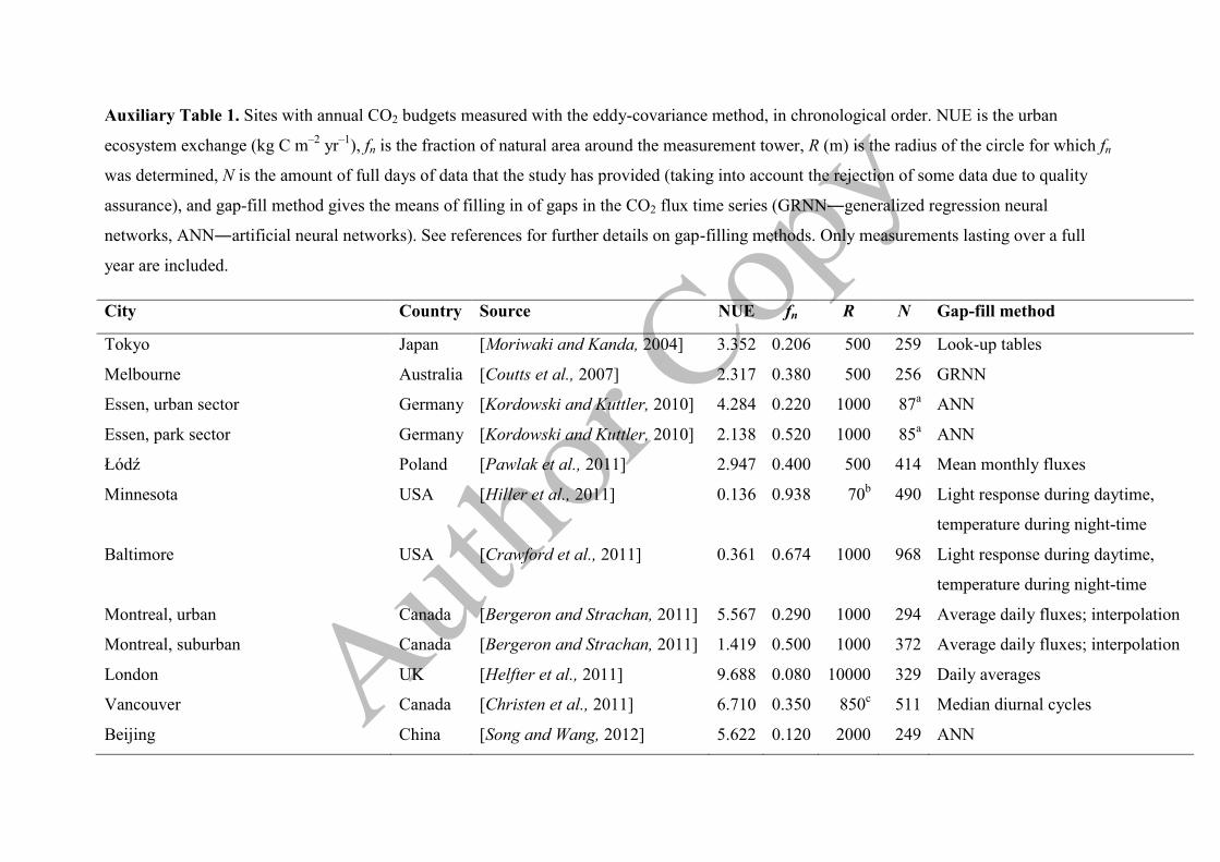
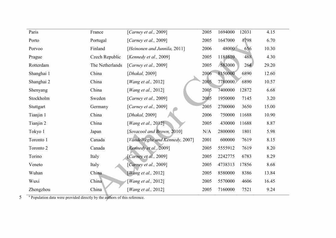
A list of 14 eddy-covariance flux towers, that provide 17 annual net urban ecosystem

exchange (NUE) estimates, is given in Auxiliary Table 1. The NUE estimates, the fraction of

natural area (fn), the radius of the circle for which fn was determined (R), and the amount of

data are all determined by original authors (exceptions are in the footnote of Auxiliary Table

1). Most of the sites are located in North America and Europe (five each), two are from

eastern Asia, and one from Australia (Auxiliary Figure 1). The measurements represent a

variety of urban forms comprising for example a highway passing a lawn [Hiller et al., 2011],

a suburban district [Crawford et al., 2011], and the densely built-up metropolitan area of

London [Helfter et al., 2011].

The values of fn range from 8% to 94% and they are equal to the vegetative fraction for

all but Baltimore and semi-urban Helsinki, but the fraction of non-vegetative surfaces (bare

soil) remains <1%. The source area of eddy-covariance measurements depends for instance

on the measurement height [Vesala et al., 2008], and thus fn values per site are given for

differently-sized areas around the measurement towers (Auxiliary Table 1). The values of R

are shown to give a view of the size of the source area of the NUE estimates, though R is not

used in the analysis as such. The data coverage for each site (N, days) was calculated by us

based on the reported measurement period and overall data rejection due to quality screening.

Only sites with all-year-around measurements were included, but N may be under a year due

to quality screening and the separation into different wind direction sectors (see e.g. Essen in

Auxiliary Table 1). The data coverage was taken into account in the exponential fit of Figure

1 in the main text by weighting data points by N(Auxiliary Table 1). The fit in is made using

the fit-function in MATLAB (Mathwoks Inc. 2012). The solution is found by non-linear

least-squares optimization, and confidence limits of the fit are provided by the function.

A list of 56 greenhouse gas (GHG) inventories is provided in Auxiliary Table 2. Four

main criteria were used in the selection of inventories: population census data must have been

provided, the research must have been conducted in the 21st century, the area in concern must

have been clearly indicated (as city, metropolitan, or county), and polygons [GADM, 2012]

for the corresponding area must be available. The latter criterion caused the rejection of

several of USA’s cities since often only county borders were available. The resulting

compilation of cities has a large variation in population: eleven of the cities have over 10

million inhabitants and ten have a population of less than a million. Where possible, an

emission value only including the effect of CO2 is given. Furthermore, if a value for

emissions that occur only within city boundaries was available, it was favored over emissions

attributable to end-use in cities (including e.g. power generation, air transport, and marine

transport). The large spectrum of methodologies behind inventory estimates is not considered

a drawback, since our NUE estimates are intended to describe the urban area as an

ecosystem, incorporating the role of vegetation. Thus, the inventory and NUE estimates can

be assumed a priori to differ due to those conceptual differences.

Statistics on countries

The regional NUE estimate for USA was made excluding Alaska and Hawaii (hence USA48),

since eddy-covariance flux sites do not characterize these areas climatologically. The

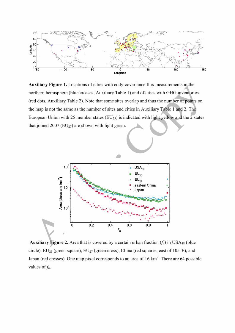
population in 2010 was 306 675 006 [U.S. Census Bureau, 2012]. The area with an urban

fraction of one in the aggregated 4 km scale data covers about 26 000 km2 (Auxiliary Figure

2). Two NUE values were calculated for the European Union: one for the 25 member states

prior to 2007 (EU25) and one for the 27 member states at present (EU27, Auxiliary Figure 1).

The population of the EU in 2011 was 502 477 005 [Eurostat, 2012], and the area covered by

complete urbanization is about 12 600 and 13 000 km2 for EU25 and EU27, respectively

(Auxiliary Figure 2). Overall, USA has a higher occurrence of very densely built-up city

centers whereas greener cities are more common in the EU. Furthermore, China has wide

areas of low urban fraction which are shown as carbon sinks in Figure 3 of the main text. The

area covered by complete urbanization is about the same in eastern China and Japan, about

5600 and 5700 km2, respectively.

2. Auxiliary discussion

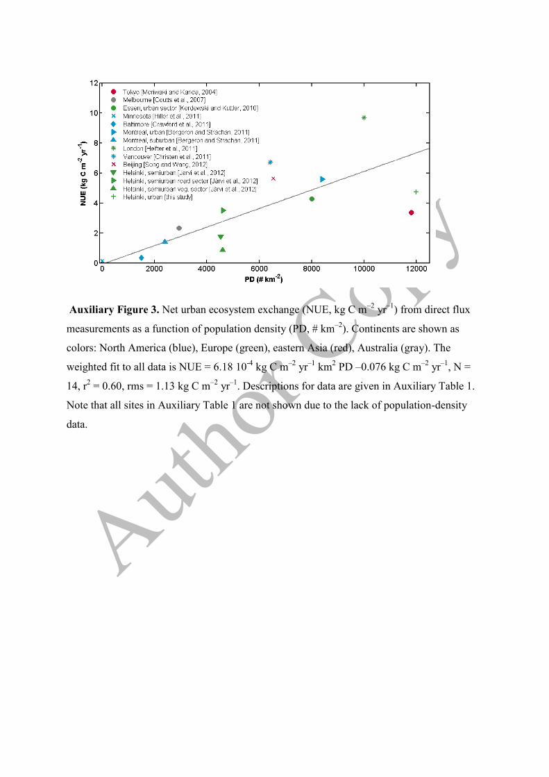
Relationship between population density and NUE

The annual NUE estimates from eddy-covariance flux measurements (Auxiliary Table 1)

grow linearly with population density, though the correspondence is not as high as with

natural fraction (Auxiliary Figure 5, r2 = 0.60, rms = 1.13 kg C m

–2 yr

–1). The dependency

does not saturate with high population density, although fuel consumption is known to be

inversely proportional to population density [Kennedy et al., 2009; Karathodorou et al.,

2010]. This might be due to a lack of eddy-covariance measurements in areas with very high

population density.

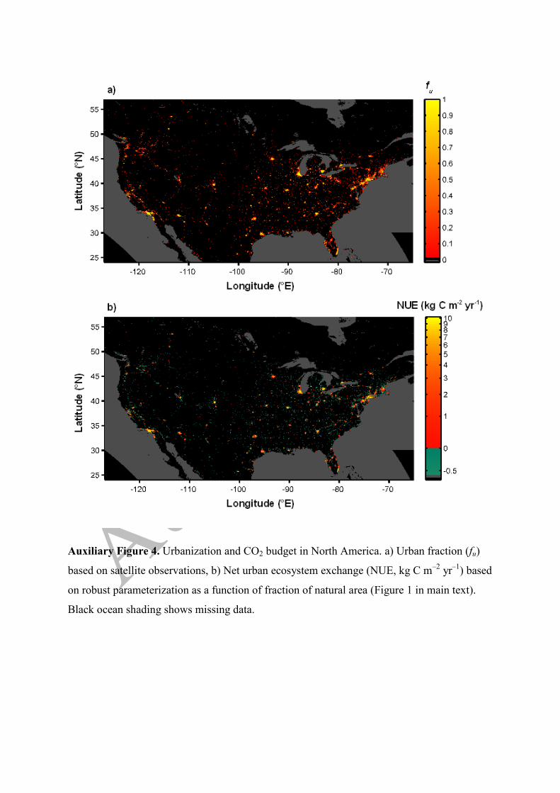
Regional estimates for NUE for North America and eastern Asia

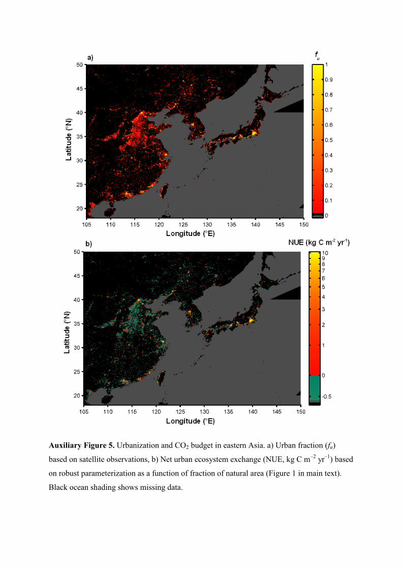
The urban fraction (fu = 1– fn) in North America and eastern Asia are depicted in Auxiliary

Figures 4a and 5a. The annual NUE estimates, based on the relationship in Figure 1 in main

text, for these regions are displayed in Auxiliary Figures 4b and 5b. For further discussion,

see section 3.2 in the main text.

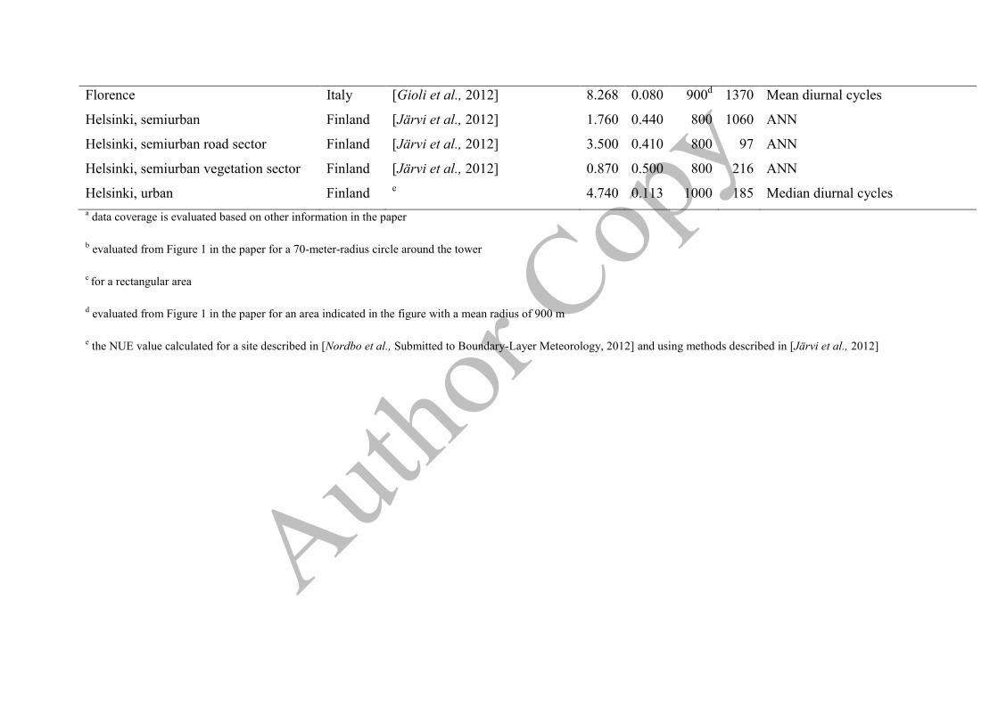
Auxiliary Table 1. Sites with annual CO2 budgets measured with the eddy-covariance method, in chronological order. NUE is the urban

ecosystem exchange (kg C m–2

yr–1

), fn is the fraction of natural area around the measurement tower, R (m) is the radius of the circle for which fn

was determined, N is the amount of full days of data that the study has provided (taking into account the rejection of some data due to quality

assurance), and gap-fill method gives the means of filling in of gaps in the CO2 flux time series (GRNN―generalized regression neural

networks, ANN―artificial neural networks). See references for further details on gap-filling methods. Only measurements lasting over a full

year are included.

City Country Source NUE fn R N Gap-fill method

Tokyo Japan [Moriwaki and Kanda, 2004] 3.352 0.206 500 259 Look-up tables

Melbourne Australia [Coutts et al., 2007] 2.317 0.380 500 256 GRNN

Essen, urban sector Germany [Kordowski and Kuttler, 2010] 4.284 0.220 1000 87a ANN

Essen, park sector Germany [Kordowski and Kuttler, 2010] 2.138 0.520 1000 85a ANN

Łódź Poland [Pawlak et al., 2011] 2.947 0.400 500 414 Mean monthly fluxes

Minnesota USA [Hiller et al., 2011] 0.136 0.938 70b 490 Light response during daytime,

temperature during night-time

Baltimore USA [Crawford et al., 2011] 0.361 0.674 1000 968 Light response during daytime,

temperature during night-time

Montreal, urban Canada [Bergeron and Strachan, 2011] 5.567 0.290 1000 294 Average daily fluxes; interpolation

Montreal, suburban Canada [Bergeron and Strachan, 2011] 1.419 0.500 1000 372 Average daily fluxes; interpolation

London UK [Helfter et al., 2011] 9.688 0.080 10000 329 Daily averages

Vancouver Canada [Christen et al., 2011] 6.710 0.350 850c 511 Median diurnal cycles

Beijing China [Song and Wang, 2012] 5.622 0.120 2000 249 ANN

Florence Italy [Gioli et al., 2012] 8.268 0.080 900d 1370 Mean diurnal cycles

Helsinki, semiurban Finland [Järvi et al., 2012] 1.760 0.440 800 1060 ANN

Helsinki, semiurban road sector Finland [Järvi et al., 2012] 3.500 0.410 800 97 ANN

Helsinki, semiurban vegetation sector Finland [Järvi et al., 2012] 0.870 0.500 800 216 ANN

Helsinki, urban Finland e 4.740 0.113 1000 185 Median diurnal cycles

a data coverage is evaluated based on other information in the paper

b evaluated from Figure 1 in the paper for a 70-meter-radius circle around the tower

c for a rectangular area

d evaluated from Figure 1 in the paper for an area indicated in the figure with a mean radius of 900 m

e the NUE value calculated for a site described in [Nordbo et al., Submitted to Boundary-Layer Meteorology, 2012] and using methods described in [Järvi et al., 2012]

Auxiliary Table 2. Cities with annual GHG budgets, based on inventories. P is the population, A is the surface area (km2), and the annual emissions 1

are given as kg of carbon per person. The emission value corresponds to equivalents of CO2 if other GHGs in addition to CO2 are included in the 2

inventory. The surface area is calculated from city border polygons [GADM, 2012]. Numbers after city names indicate multiple studies from the same 3

urban area. Note that studies with same urban-area name may be for different areas (e.g. core city versus metropolitan area). 4

City Country Source Study

year

P A

(km2)

Emissions

(kg C yr–1

P–1

)

Athens Greece [Carney et al., 2009] 2005 3997006 3863 9.50

Bangkok 1 Thailand [Kennedy et al., 2009] 2005 5658953 1570 4.80

Bangkok 2 Thailand [Croci et al., 2011]a 2007 5658953 1570 7.55

Barcelona Spain [Kennedy et al., 2009] 2006 1605602 100 2.40

Beijing 1 China [Dhakal, 2009] 2006 5810000 16388 9.00

Beijing 2 China [Sovacool and Brown, 2010] N/A 2000000 1360 4.33

Beijing 3 China [Wang et al., 2012] 2005 5380000 16388 8.62

Bologna Italy [Carney et al., 2009] 2005 900000 3696 9.10

Brussels Belgium [Carney et al., 2009] 2005 1006749 156 7.20

Chongqing 1 China [Dhakal, 2009] 2006 8080000 82532 3.70

Chongqing 2 China [Wang et al., 2012] 2005 7980000 82532 2.88

Denver 1 USA [Ramaswami et al., 2008] 2005 579744 403 18.90

Denver 2 USA [Kennedy et al., 2009] 2005 579744 403 21.50

Denver 3 USA [Hillman and Ramaswami, 2010] 2005 579744 403 17.88

District of Columbia USA [Dodman, 2009] 2005 573604 166 19.70

Frankfurt Rhein-Main Germany [Carney et al., 2009] 2005 3761700 7371 12.65

Glasgow and Clyde Valley 1 UK [Dodman, 2009] 2004 1747000 3365 8.40

Glasgow and Clyde Valley 2 UK [Carney et al., 2009] 2004 1750000 3365 7.34

Guangzhou China [Wang et al., 2012] 2005 9580000 7153 7.86

Hamburg Germany [Carney et al., 2009] 2005 4300000 19076 8.17

Hangzhou China [Wang et al., 2012] 2005 7500000 17089 9.87

Helsinki 1 Finland [Carney et al., 2009] 2005 988500 762 6.70

Helsinki 2 Finland [Heinonen and Junnila, 2011] 2006 550000 173 13.20

Lanzhou China [Wang et al., 2012] 2005 3140000 13267 21.04

London 1 UK [Kennedy et al., 2009] 2003 7364100 1601 9.60

London 2 UK [Dodman, 2009] 2006 7145161 1601 6.20

London 3 UK [Sovacool and Brown, 2010] N/A 8000000 1601 4.37

London 4 UK [Croci et al., 2011] 2003 7379700 1601 5.76

Los Angeles USA [Kennedy et al., 2009] 2000 9519338 10590 13.00

Madrid 1 Spain [Carney et al., 2009] 2005 5938902 8022 6.28

Madrid 2 Spain [Croci et al., 2011] 2004 2938723 605 4.98

Milan Italy [Croci et al., 2011] 2005 1298196 181 5.43

Nanjing 1 China [Bi et al., 2011] 2009 7713100 6592 9.78

Nanjing 2 China [Wang et al., 2012] 2005 6680000 6592 7.71

Oslo Norway [Carney et al., 2009] 2005 1100000 5367 3.00

Osrednjeslovenska Slovenia [Carney et al., 2009] 2005 492100 2540 8.77

Paris France [Carney et al., 2009] 2005 1694000 12031 4.15

Porto Portugal [Carney et al., 2009] 2005 1647000 1798 6.70

Porvoo Finland [Heinonen and Junnila, 2011] 2006 48000 656 10.30

Prague Czech Republic [Kennedy et al., 2009] 2005 1181610 488 4.30

Rotterdam The Netherlands [Carney et al., 2009] 2005 583000 264 29.20

Shanghai 1 China [Dhakal, 2009] 2006 8150000 6890 12.60

Shanghai 2 China [Wang et al., 2012] 2005 7780000 6890 10.57

Shenyang China [Wang et al., 2012] 2005 7400000 12872 6.68

Stockholm Sweden [Carney et al., 2009] 2005 1950000 7145 3.20

Stuttgart Germany [Carney et al., 2009] 2005 2700000 3650 15.00

Tianjin 1 China [Dhakal, 2009] 2006 750000 11688 10.90

Tianjin 2 China [Wang et al., 2012] 2005 430000 11688 8.87

Tokyo 1 Japan [Sovacool and Brown, 2010] N/A 2800000 1801 5.98

Toronto 1 Canada [VandeWeghe and Kennedy, 2007] 2001 600000 7619 8.15

Toronto 2 Canada [Kennedy et al., 2009] 2005 5555912 7619 8.20

Torino Italy [Carney et al., 2009] 2005 2242775 6783 8.29

Veneto Italy [Carney et al., 2009] 2005 4738313 17856 8.68

Wuhan China [Wang et al., 2012] 2005 8580000 8386 13.84

Wuxi China [Wang et al., 2012] 2005 5570000 4606 16.45

Zhengzhou China [Wang et al., 2012] 2005 7160000 7521 9.24

a Population data were provided directly by the authors of this reference. 5

Auxiliary Figure 1. Locations of cities with eddy-covariance flux measurements in the

northern hemisphere (blue crosses, Auxiliary Table 1) and of cities with GHG inventories

(red dots, Auxiliary Table 2). Note that some sites overlap and thus the number of points on

the map is not the same as the number of sites and cities in Auxiliary Table 1 and 2. The

European Union with 25 member states (EU25) is indicated with light yellow and the 2 states

that joined 2007 (EU27) are shown with light green.

Auxiliary Figure 2. Area that is covered by a certain urban fraction (fu) in USA48 (blue

circle), EU25 (green square), EU27 (green cross), China (red squares, east of 105°E), and

Japan (red crosses). One map pixel corresponds to an area of 16 km2. There are 64 possible

values of fu.

Auxiliary Figure 3. Net urban ecosystem exchange (NUE, kg C m–2

yr–1

) from direct flux

measurements as a function of population density (PD, # km–2

). Continents are shown as

colors: North America (blue), Europe (green), eastern Asia (red), Australia (gray). The

weighted fit to all data is NUE = 6.18 10-4

kg C m–2

yr–1

km2 PD –0.076 kg C m

–2 yr

–1, N =

14, r2 = 0.60, rms = 1.13 kg C m

–2 yr

–1. Descriptions for data are given in Auxiliary Table 1.

Note that all sites in Auxiliary Table 1 are not shown due to the lack of population-density

data.

Auxiliary Figure 4. Urbanization and CO2 budget in North America. a) Urban fraction (fu)

based on satellite observations, b) Net urban ecosystem exchange (NUE, kg C m–2

yr–1

) based

on robust parameterization as a function of fraction of natural area (Figure 1 in main text).

Black ocean shading shows missing data.

Auxiliary Figure 5. Urbanization and CO2 budget in eastern Asia. a) Urban fraction (fu)

based on satellite observations, b) Net urban ecosystem exchange (NUE, kg C m–2

yr–1

) based

on robust parameterization as a function of fraction of natural area (Figure 1 in main text).

Black ocean shading shows missing data.

References

Bergeron, O. and I. B. Strachan (2011), CO2 sources and sinks in urban and suburban areas

of a northern mid-latitude city, Atmos. Environ., 45, 1564-1573.

Bi, J., R. Zhang, H. Wang, M. Liu, and Y. Wu (2011), The benchmarks of carbon emissions

and policy implications for China's cities: Case of Nanjing, Energy Policy, 39, 4785-4794.

Carney, S., N. W. Green R., and R. Read (2009), Greenhouse gas emissions inventories for

18 European regions, EU CO2 80/50 Project Stage 1: Inventory Formation., The Greenhouse

Gas Regional Inventory Protocol (GRIP).

Christen, A., N. C. Coops, B. R. Crawford, R. Kellett, K. N. Liss, I. Olchovski, T. R. Tooke,

M. van der Laan, and J. A. Voogt (2011), Validation of modeled carbon-dioxide emissions

from an urban neighborhood with direct eddy-covariance measurements, Atmos. Environ., 45,

6057-6069.

Coutts, A. M., J. Beringer, and N. J. Tapper (2007), Characteristics influencing the variability

of urban CO2 fluxes in Melbourne, Australia, Atmos. Environ., 41, 51-62.

Crawford, B., C. S. B. Grimmond, and A. Christen (2011), Five years of carbon dioxide

fluxes measurements in a highly vegetated suburban area, Atmos. Environ., 45, 896-905.

Croci, E., S. Melandri, and T. Molteni (2011), Determinants of cities' GHG emissions: a

comparison of seven global cities, Int. J. Clim. Chang. Strateg. Manag., 3, 275-301.

Dhakal, S. (2009), Urban energy use and carbon emissions from cities in China and policy

implications, Energy Policy, 37, 4208-4219.

Dodman, D. (2009), Blaming cities for climate change? An analysis of urban greenhouse gas

emissions inventories, Environ. Urban., 21, 185-201.

Eurostat (2012), Population at 1 January,

http://epp.eurostat.ec.europa.eu/tgm/table.do?tab=table&language=en&pcode=tps00001&tabl

eSelection=1&footnotes=yes&labeling=labels&plugin=1.

GADM (2012), Database of Global Administrative Areas, www.gadm.org.

Gioli, B., P. Toscano, E. Lugato, A. Matese, F. Miglietta, A. Zaldei, and F. P. Vaccari (2012),

Methane and carbon dioxide fluxes and source partitioning in urban areas: The case study of

Florence, Italy, Environ. Pollut., 164, 125-131.

Heinonen, J. and S. Junnila (2011), Case study on the carbon consumption of two

metropolitan cities, Int. J. Life Cycle Assess., 16, 569-579.

Helfter, C., D. Famulari, G. J. Phillips, J. F. Barlow, C. R. Wood, C. S. B. Grimmond, and E.

Nemitz (2011), Controls of carbon dioxide concentrations and fluxes above central London,

Atmos. Chem. Phys., 11, 1913-1928.

Hiller, R. V., J. P. McFadden, and N. Kljun (2011), Interpreting CO2 Fluxes Over a Suburban

Lawn: The Influence of Traffic Emissions, Bound. -Layer Meteorol., 138, 215-230.

Hillman, T. and A. Ramaswami (2010), Greenhouse Gas Emission Footprints and Energy

Use Benchmarks for Eight US Cities, Environ. Sci. Technol., 44, 1902-1910.

Järvi, L., A. Nordbo, H. Junninen, A. Riikonen, J. Moilanen, E. Nikinmaa, and T. Vesala

(2012), Seasonal and annual variation of carbon dioxide surface fluxes in Helsinki, Finland,

in 2006-2010, Atmos. Chem. Phys. Discuss., 12, 8355-8396.

Karathodorou, N., D. J. Graham, and R. B. Noland (2010), Estimating the effect of urban

density on fuel demand, Energy Econ., 32, 86-92.

Kennedy, C., J. Steinberger, B. Gasson, Y. Hansen, T. Hillman, M. Havranek, D. Pataki, A.

Phdungsilp, A. Ramaswami, and G. Villalba Mendez (2009), Greenhouse Gas Emissions

from Global Cities, Environ. Sci. Technol., 43, 7297-7302.

Kordowski, K. and W. Kuttler (2010), Carbon dioxide fluxes over an urban park area, Atmos.

Environ., 44, 2722-2730.

MathWorks Inc , MATLAB, 2012a.

Moriwaki, R. and M. Kanda (2004), Seasonal and diurnal fluxes of radiation, heat, water

vapor, and carbon dioxide over a suburban area, J. Appl. Meteorol., 43, 1700-1710.

Nordbo, A., L. Järvi, S. Haapanala, J. Moilanen, and T. Vesala (Submitted to Boundary-

Layer Meteorology, 2012), Intra-city variation in urban morphology and turbulence structure

in Helsinki, Finland.

Pawlak, W., K. Fortuniak, and M. Siedlecki (2011), Carbon dioxide flux in the centre of

Łódź, Poland - analysis of a 2-year eddy covariance measurement data set, Int. J. Climatol.,

31, 232-243.

Ramaswami, A., T. Hillman, B. Janson, M. Reiner, and G. Thomas (2008), A demand-

centered, hybrid life-cycle methodology for city-scale greenhouse gas inventories, Environ.

Sci. Technol., 42, 6455-6461.

Song, T. and Y. Wang (2012), Carbon dioxide fluxes from an urban area in Beijing, Atmos.

Res., 106, 139-149.

Sovacool, B. K. and M. A. Brown (2010), Twelve metropolitan carbon footprints: A

preliminary comparative global assessment, Energy Policy, 38, 4856-4869.

U.S. Census Bureau (2012), State & County QuickFacts,

http://quickfacts.census.gov/qfd/states.

VandeWeghe, J. R. and C. Kennedy (2007), A spatial analysis of residential greenhouse gas

emissions in the Toronto Census Metropolitan Area, J. Ind. Ecol., 11, 133-144.

Vesala, T., N. Kljun, Ü. Rannik, J. Rinne, A. Sogachev, T. Markkanen, K. Sabelfeld, T.

Foken, and M. Y. Leclerc (2008), Flux and concentration footprint modelling: State of the

art, Environ. Pollut., 152, 653-666.

Wang, H., J. Bi, R. Zhang, and M. Liu (2012), The carbon emissions of Chinese cities,

Atmos. Chem. Phys. Discuss., 12, 7985-8007.