Fractional Abelian topological phases of matter for fermions in two-dimensional space Christopher Mudry Condensed Matter Theory Group, Paul Scherrer Institute, CH-5232 Villigen PSI, Switzerland
Transcript
Fractional Abelian topological phases ofmatter for fermions in two-dimensional
space
Christopher MudryCondensed Matter Theory Group, Paul Scherrer Institute, CH-5232 Villigen PSI, Switzerland
Contents
1 Introduction 1
2 The tenfold way in quasi-one-dimensional space 112.1 Symmetries for the case of one one-dimensional channel 112.2 Symmetries for the case of two one-dimensional channels 162.3 Definition of the minimum rank 182.4 Topological spaces for the normalized Dirac masses 20
3 Fractionalization from Abelian bosonization 223.1 Introduction 223.2 Definition 223.3 Chiral equations of motion 233.4 Gauge invariance 243.5 Conserved topological charges 273.6 Quasi-particle and particle excitations 293.7 Bosonization rules 323.8 From the Hamiltonian to the Lagrangian formalism 353.9 Applications to polyacetylene 37
4 Stability analysis for the edge theory in the symmetry class AII 404.1 Introduction 404.2 Definitions 444.3 Time-reversal symmetry of the edge theory 464.4 Pinning the edge fields with disorder potentials: the Haldane criterion 484.5 Stability criterion for edge modes 494.6 The stability criterion for edge modes in the FQSHE 51
5 Construction of two-dimensional topological phases from coupled wires 535.1 Introduction 535.2 Definitions 565.3 Strategy for constructing topological phases 615.4 Reproducing the tenfold way 645.5 Fractionalized phases 735.6 Summary 79
References 81
1
Introduction
During these lectures, I will focus exclusively on two-dimensional realizations of frac-tional topological insulators. However, before doing so, I need to revisit the definition ofnon-interacting topological phases of matter for fermions and, for this matter, I would liketo attempt to place some of the recurrent concepts that have been used during this school on atime line that starts in 1931.
Topology in physics enters the scene in 1931 when Dirac showed that the existence ofmagnetic monopoles in quantum mechanics implies the quantization of the electric and mag-netic charge. [24]
In the same decade, Tamm and Shockley surmised from the band theory of Bloch thatsurface states can appear at the boundaries of band insulators (see Fig. 1.1). [115, 110]
The dramatic importance of static and local disorder for electronic quantum transport hadbeen overlooked until 1957 when Anderson showed that sufficiently strong disorder “gener-ically” localizes a bulk electron. [5] That there can be exceptions to this rule follows fromreinterpreting the demonstration by Dyson in 1953 that disordered phonons in a linear chaincan acquire a diverging density of states at zero energy with the help of bosonization tools inone-dimensional space (see Fig. 1.2). [25]
Following the proposal by Wigner to model nuclear interactions with the help of randommatrix theory, Dyson introduced the threefold way in 1963, [26] i.e., the study of the jointprobability distribution
P (θ1, · · · , θN ) ∝∏
1≤j<k≤N
∣∣eiθj − eiθk∣∣β , β = 1, 2, 4, (1.1)
for the eigenvalues of unitary matrices of rank N generated by random Hamiltonians withoutany symmetry (β = 2), by random Hamiltonians with time-reversal symmetry correspond-ing to spin-0 particles (β = 1), and by random Hamiltonians with time-reversal symmetrycorresponding to spin-1/2 particles (β = 4).
Topology acquired a mainstream status in physics as of 1973 with the disovery of Berezin-skii and of Kosterlitz and Thousless that topological defects in magnetic classical textures candrive a phase transition. [9, 66, 65] In turn, there is an intimate connection between topo-logical defects of classical background fields in the presence of which electrons propagateand fermionic zero modes, as was demonstrated by Jackiw and Rebbi in 1976 (see Fig.1.3). [51, 114]
The 70’s witnessed the birth of lattice gauge theory as a mean to regularize quantum chro-modynamics (QCD4). Regularizing the standard model on the lattice proved to be more diffi-cult because of the Nielsen-Ninomiya no-go theorem that prohibits defining a theory of chiral
2 Introduction
Fig. 1.1 Single-particle spectrum of a Bogoliubov-de-Gennes superconductor in a cylindrical geometrywhich is the direct sum of a px + ipy and of a px − ipy superconductor (after P-Y. Chang, C. Mudry,and S. Ryu, arXiv:1403.6176). The two-fold degenerate dispersion of two chiral edge states are seen tocross the mean-field superconducting gap. There is a single pair of Kramers degenerate edge state thatdisperses along one edge of the cylinder.
(a) (b)
Fig. 1.2 (a) The beta function of the dimensionless conductance g is plotted (qualitatively) as a functionof the linear system size L in the orthogonal symmetry class (β = 1) when space is of dimensionalityd = 1, d = 2, and d = 3, respectively. (b) The dependence of the mean Landauer conductance 〈g〉for a quasi-one-dimensional wire as a function of the length of the wire L in the symmetry class BD1.The number N of channel is varied as well as the chemical potential ε of the leads. [Taken from P. W.Brouwer, A. Furusaki, C. Mudry, S. Ryu, BUTSURI 60, 935 (2005)]
fermions on a lattice in odd-dimensional space without violating locality or time-reversal sym-metry. [90,89,91] This is known as the fermion-doubling problem when regularizing the Diracequation in d-dimensional space on a d-dimensional lattice.
The 80’s opened with a big bang. The integer quantum Hall effect (IQHE) was discoveredin 1980 by von Klitzing, Dorda, and Pepper (see Fig. 1.4), [63] while the fractional quantumHall effect (FQHE) was discovered in 1982 by Tsui, Stormer, and Gossard. [118] At inte-ger fillings of the Landau levels, the non-interacting ground state is unique and the screenedCoulomb interaction Vint can be treated perturbatively, as long as transitions between Landaulevels or outside the confining potential Vconf along the magnetic field are suppressed by the
Introduction 3
(a)
������
������
(b)+π/2−π/2
k
ε (k)
Fig. 1.3 (a) Nearest-neighbor hopping of a spinless fermion along a ring with a real-valued hoppingamplitude that is larger on the thick bonds than on the thin bonds. There are two defective sites, each ofwhich are shared by two thick bonds. (b) The single-particle spectrum is gapped at half-filling. There aretwo bound states within this gap, each exponentially localized around one of the defective sites, whoseenergy is split from the band center by an energy that decreases exponentially fast with the separation ofthe two defects.
single-particle gaps ~ωc and Vconf , respectively,
Vint � ~ωc � Vconf , ωc = eB/(mc). (1.2)
When Galilean invariance is not broken, the conductivity tensor is then given by the classicalDrude formula
limτ→∞
j =
(0 + (BRH)
−1
− (BRH)−1
0
)E, R−1
H ..= −n e c, (1.3)
that relates the (expectation value of the) electronic current density j ∈ R2 to an appliedelectric field E ∈ R2 within the plane perpendicular to the applied static and uniform mag-netic field B in the ballistic regime (τ → ∞ is the scattering time). The electronic density,the electronic charge, and the speed of light are denoted n, e, and c, respectively. Moderatedisorder is an essential ingredient to observe the IQHE, for it allows the Hall conductivityto develop plateaus at sufficiently low temperatures that are readily visible experimentally(see Fig. 1.4). These plateaus are a consequence of the fact that most single-particle statesin a Landau level are localized by disorder, according to Anderson’s insight that any quan-tum interference induced by a static and local disorder almost always lead to localization inone- and two-dimensional space. The caveat “almost” is crucial here, for the very observationof transitions between Landau plateaus implies that not all single-particle Landau levels arelocalized.
The explanation for the integer quantum Hall effect followed quickly its discovery owingto a very general argument of Laughlin based on gauge invariance that implies that the Hallconductivity must take a fractional value if the longitudinal conductivity vanishes (mobilitygap). [67] This argument was complemented by an argument of Halperin stressing the crucialrole played by edge states when electrons in the quantum Hall effect are confined to a stripgeometry (see Fig. 1.5), [47] while works from Thouless, Kohmoto, Nightingale, den Nijs and
4 Introduction
(a) (b) (c)
Fig. 1.4 (a) The Hall conductivity is a linear function of the electron density if Galilean invari-ance holds. (b) Galilean invariance is broken in the presence of disorder so that plateaus becomeevident at integral filling fractions of the Landau levels. (c) Graphene deposited on SiO2/Si, T=1.6K and B=9 T (inset T=30 mK) support the integer quantum Hall effect at the filling fractionsν = ±2,±6,±10, · · · = ±2(2n + 1), n ∈ N. [Taken from Zhang et al., Nature 438, 201 (2005)]
Niu demonstrated that the Hall response is, within linear response theory, proportional to thetopological invariant
C ..= − i
2π
2π∫0
dφ
2π∫0
dϕ
[⟨∂Ψ
∂φ
∣∣∣∣ ∂Ψ
∂ϕ
⟩−⟨∂Ψ
∂ϕ
∣∣∣∣ ∂Ψ
∂φ
⟩](1.4)
that characterizes the many-body ground state |Ψ〉 obeying twisted boundary conditions inthe quantum Hall effect. [117, 111, 92, 93] Together, these arguments constitute the first ex-ample of the bulk-edge correspondence with observable consequences, namely the distinctivesignatures of both the integer and the fractional quantum Hall effect.
The transitions between plateaus in the quantum Hall effect are the manifestations at fi-nite temperature and for a system of finite size of a continuous quantum phase transition,i.e., of a singular dependence of the conductivity tensor on the magnetic field (filling frac-tion) that is rounded by a non-vanishing temperature or by the finite linear size of a sample.In the non-interacting limit, as was the case for the Dyson singularity at the band center, anisolated bulk single-particle state must become critical in the presence of not-too strong dis-order. The one-parameter scaling theory of Anderson localization that had been initiated byWegner and was encoded by a class on non-linear-sigma models (NLSMs) has to be incom-plete. [123,3,50] Khmelnitskii, on the one hand, and Levine, Libby, and Pruisken, on the otherhand, introduced in 1983 a two-parameter scaling theory for the IQHE on phenomenologicalgrounds. [57, 71, 96] They also argued that the NLSM for the IQHE, when augmented by atopological θ term, would reproduce the two-parameter flow diagram (see Fig. 1.6). This re-markable development took place simultaneously with the works on Haldane on encoding thedifference between half-integer and integer spin chains (Haldane’s conjecture) by the presenceof a θ = π topological term in the O(3) NLSM [42, 44] and by the work of Witten [130] onprincipal chiral models augmented by a Wess-Zumino-Novikow-Witten (WZNW) term.
Deciphering the critical theory for the plateau transition is perhaps the most tantalizingchallenge in the theory of Anderson localization. Among the many interesting avenues thathave been proposed to reach this goal (that remains elusive so far), Ludwig, Fisher, Shankar,and Grinstein studied random Dirac fermions in two-dimensional space in 1994 (see Fig.1.7), [75] motivated as they were by the fact that a massive Dirac fermion in two-dimensionalspace carries the fractional value
Introduction 5
B
x
y
z
(a) (b) (c)
Integer Quantum Hall Effect
Fig. 1.5 Chiral edges are immune to backscattering within each traffic lane.
σDiracH = ±1
2
e2
h(1.5)
according to Deser, Jackiw, and Templeton [23] and that it is possible to regularize two suchmassive Dirac fermions on a two-band lattice model realizing a Chern insulator according toHaldane. [45]
The early 90’s were also the golden age of mesoscopic physics, the application of randommatrix theory to condensed matter physics. The threefold way had been applied successfully toquantum dots and quantum transport in quasi-one-dimensional geometries. Zirnbauer in 1996and Altland and Zirnbauer in 1997 extended the threefold way of Dyson to the tenfold way byincluding three symmetry classes of relevance to quantum chromodynamics called the chiralclasses, and four symmetry classes of relevance to superconducting quantum dots (see Table1.1). [133, 4, 49] Quantum transport in quasi-one-dimensional wires belonging to the chiraland superconducting classes was studied by Brouwer, Mudry, Simons, and Altland and byBrouwer, Furusaki, Gruzberg, Mudry, respectively (see Fig. 1.8). [15,14,12,13] Unlike in thethreefold way, the three chiral symmetry classes and two of the four superconducting classes(the symmetry classes D and DIII) were shown to realize quantum critical point separatinglocalized phases in quasi-one-dimensional arrays of wires. The diverging nature of the densityof states at the band center (the disorder is of vanishing mean) for five of the ten symmetryclasses in Table 1.2 is a signature of topologically protected zero modes bound to point defects.These point defects are vanishing values of an order parameter (domain walls) responsible ofa spectral if translation symmetry was restored.
Lattice realizations of Z2 topological band insulators in two-dimensional space were pro-posed by Kane and Mele in Refs. [54,55] and in three-dimensional space by Refs. [81,99,35].This theoretical discovery initiated in Refs. [102, 101] the search of Dirac Hamiltonians be-longing to the two-dimensional symmetry classes AII and CII from Table 1.1 for which thecorresponding NLSM encoding the effects of static and local disorder were augmented by atopological term so as to evade Anderson localization on the boundary of a d = 3-dimensionaltopological insulators. Following this route for all symmetry classes and for all dimensions,Ryu, Schnyder, Furusaki, and Ludwig arrived at the periodic Table 1.3. [106, 107, 103] Thesame table was derived independently by Kitaev using a mathematical construction known asK theory that he applied to gapped Hamiltonians in the bulk (upon the imposition of periodicboundary conditions, say) in the clean limit. [58] This table specifies in any given dimensiond of space, for which symmetry classes it is possible to realize a many-body ground statefor non-interacting fermions subject to a static and local disorder such that all bulk states
6 Introduction
(a)g g
O(3) NLSM O(3) NLSM+
SU(2)
θ=π
1 (b)
Fig. 1.6 (a) A topological θ = π term modifies the RG flow to strong coupling in the two-dimensionalO(3) non-linear-sigma model. There exists a stable critical point at intermediary coupling that realizesthe conformal field theory SU(2)1. (b) Pruisken argues that the phenomenological two-parameter flowdiagram of Khmelnitskii is a consequence of augmenting the NLSM in the unitary symmetry class by atopological term.
are localized but there exist a certain (topological) number of boundary states, that remaindelocalized.
The goals of these lectures are the following.• First, I would like to rederive the tenfold way for non-interacting fermions in the presence
of local interactions and static local disorder.• Second, I would like to decide if interactions between fermions can produce topological
phases of matter with protected boundary states that are not captured by the tenfold way.This program will be applied in two-dimensional space.
These lectures are organized as follows. Section 2 motivates the tenfold way by derivingit explicitly in quasi-one-dimensional space. Section 3 is a review of Abelian chiral bosoniza-tion, the technical tool that allows one to go beyond the tenfold way so as to incorporate theeffects of many-body interactions. Abelian chiral bosonization is applied in Sec. 4 to demon-strate the stability of the gapless helical edge states in the symmetry class AII in the presenceof disorder and many-body interactions. Abelian chiral bosonization is applied in Sec. 5 toconstruct microscopically long-ranged entangled phases of two-dimensional quantum matter.
Introduction 7
(a) (b)
AIII
AII
D
IQHE
(c) (d)
Fig. 1.7 (a) A single (non-degenerate) cone of Dirac fermions in two-dimensional space realizes acritical point between two massive phases of Dirac fermions, each of which carries the Hall conductanceσDirac
H = ±(1/2) in units of e2/h. (b) A generic static and local random perturbation of a single Diraccone is encoded by three channels. There is a random vector potential that realizes the symmetry classAIII if it is the only one present. There is a random scalar potential that realizes the symmetry classAII if it is the only one present. There is a random mass that realizes the symmetry class D if it isthe only one present. It is conjectured in Ref. [75] that in the presence of all three channels, the RGflow to strong coupling (the variance of the disorder in each channel) is to the plateau transition in theuniversality class of the IQHE. (c) Unit cell of the honeycomb lattice with the pattern of nearest- andnext-nearest-neighbor hopping amplitude that realizes a Chen insulators with two bands, shown in panel(d), each of which carries the Chern number ±1.
Fig. 1.8 (Taken from Ref. [13]) The “radial coordinate” of the transfer matrixM from Table 1.2 makesa Brownian motion on an associated non-compact symmetric space.
8 Introduction
Table 1.1 Listed are the ten Altland-Zirnbauer (AZ) symmetry classes of single-particle HamiltoniansH, classified according to their behavior under time-reversal symmetry (T ), charge-conjugation (or:particle-hole) symmetry (C), as well as “sublattice” (or: “chiral”) symmetry (S). The labels T, C, andS, represent the presence/absence of time-reversal, particle-hole, and chiral symmetries, respectively, aswell as the types of these symmetries. These operations square to either ± times the unit operator whenthey are symmetries. The number 0 indicates that these operations are not symmetries. The columnentitled “Hamiltonian” lists, for each of the ten AZ symmetry classes, the symmetric space of which thequantum mechanical time-evolution operator exp(itH) is an element. The column “Cartan label” is thename given to the corresponding symmetric space listed in the column “Hamiltonian” in Elie Cartan’sclassification scheme (dating back to the year 1926). The last column entitled “G/H (fermionic NLSM)”lists the (compact sectors of the) target space of the NLSM describing Anderson localization physics atlong wavelength in this given symmetry class.
Cartan label T C S Hamiltonian G/H (fermionic NLSM)
Table 1.2 Altland-Zirnbauer (AZ) symmetry classes for disordered quantum wires. Symmetry classesare defined by the presence or absence of time-reversal symmetry (TRS) and spin-rotation symmetry(SRS), and by the single-particle spectral symmetries of sublattice symmetry (SLS) (random hoppingmodel at the band center) also known as chiral symmetries, and particle-hole symmetry (PHS) (ze-ro-energy quasiparticles in superconductors). For historical reasons, the first three rows of the table arereferred to as the orthogonal (O), unitary (U), and symplectic (S) symmetry classes when the disorderis generic. The prefix “ch” that stands for chiral is added when the disorder respects a SLS as in thenext three rows. Finally, the last four rows correspond to dirty superconductors and are named after thesymmetric spaces associated to their Hamiltonians. The table lists the multiplicities of the ordinary andlong rootsmo± andml of the symmetric spaces associated with the transfer matrix. Except for the threechiral classes, one has mo+ = mo− = mo. For the chiral classes, one has mo+ = 0, mo− = mo.The table also lists the degeneracy D of the transfer matrix eigenvalues, as well as the symbols for thesymmetric spaces associated to the transfer matrixM and the Hamiltonian H. Let g denote the dimen-sionless Landauer conductance and let ρ(ε) denote the (self-averaging) density of states (DOS) per unitenergy and per unit length. The last three columns list theoretical results for the weak-localization cor-rection δg for ` � L � N` the disorder average ln g of ln g for L � N`, and the DOS near ε = 0.The results for ln g and ρ(ε) in the chiral classes refer to the case of N even. For odd N , ln g and ρ(ε)
are the same as in class D.
Symmetry class mo ml D M H δg −ln g ρ(ε) for 0 < ετc � 1AI 1 1 2 CI AI −2/3 2L/(γ`) ρ0A 2 1 2(1) AIII A 0 2L/(γ`) ρ0
Table 1.3 Classification of topological insulators and superconductors as a function of spatial dimen-sion d and AZ symmetry class, indicated by the “Cartan label” (first column). The definition of the tenAZ symmetry classes of single particle Hamiltonians is given in Table 1.1. The symmetry classes aregrouped in two separate lists – the complex and the real cases, respectively – depending on whetherthe Hamiltonian is complex, or whether one (or more) reality conditions (arising from time-reversal orcharge-conjugation symmetries) are imposed on it; the AZ symmetry classes are ordered in such a waythat a periodic pattern in dimensionality becomes visible. [58] The symbols Z and Z2 indicate that thetopologically distinct phases within a given symmetry class of topological insulators (superconductors)are characterized by an integer invariant (Z), or a Z2 quantity, respectively. The symbol “0” denotes thecase when there exists no topological insulator (superconductor), i.e., when all quantum ground statesare topologically equivalent to the trivial state.
Real case
Cartan\d 0 1 2 3 4 5 6 7 8 9 10 11 · · ·A Z 0 Z 0 Z 0 Z 0 Z 0 Z 0 · · ·
This section is dedicated to a non-vanishing density of non-interacting fermions hoppingbetween the sites of quasi-one-dimensional lattices or between the sites defining the one-dimensional boundary of a two-dimensional lattice. According to the Pauli exclusion princi-ple, the non-interacting ground state is obtained by filling all the single-particle energy eigen-states up to the Fermi energy fixed by the fermion density. The fate of this single-particleenergy eigenstate when a static and local random potential is present is known as the problemof Anderson localization. The effect of disorder on a single-particle extended energy eigen-state state can be threefold:• The extended nature of the single-particle energy eigenstate is robust to disorder.• The extended single-particle energy eigenstate is turned into a critical state.• The extended single-particle energy eigenstate is turned into a localized state.
There are several methods allowing to decide which one of these three outcomes takes place.Irrespectively of the dimensionality d of space, the symmetries obeyed by the static and lo-cal random potential matter for the outcome in a dramatic fashion. To illustrate this point, Iconsider the problem of Anderson localization in quasi-one-dimensional space.
2.1 Symmetries for the case of one one-dimensional channel
For simplicity, consider first the case of an infinitely long one-dimensional chain with thelattice spacing a ≡ 1 along which a non-vanishing but finite density of spinless fermions hopwith the uniform nearest-neighbor hopping amplitude t. If periodic boundary conditions areimposed, the single-particle Hamiltonian is the direct sum over all momenta −π ≤ k ≤ +πwithin the first Brillouin zone of
H(k) ..= −2t cos k. (2.1)
The Fermi energy εF intersects the dispersion (2.1) at the two Fermi points±kF. Linearizationof the dispersion (2.1) about these two Fermi points delivers the Dirac Hamiltonian
HD ..= −τ3 i∂
∂x(2.2a)
in the units defined by~ ≡ 1, vF = 2t | sin kF| ≡ 1. (2.2b)
Here, τ3 is the third Pauli matrices among the four 2× 2 matrices
12 The tenfold way in quasi-one-dimensional space
τ0 ..=(
1 00 1
), τ1 ..=
(0 11 0
), τ2 ..=
(0 −i
+i 0
), τ3 ..=
(+1 00 −1
). (2.2c)
The momentum eigenstate
ΨR,p(x) ..= e+ip x
(10
)(2.3a)
is an eigenstate with the single-particle energy εR(p) = +p. The momentum eigenstate
ΨL,p(x) ..= e+ip x
(01
)(2.3b)
is an eigenstate with the single-particle energy εL(p) = −p. The plane waves
ΨR,p(x, t) ..= e+ip (x−t)(
10
)(2.4a)
and
ΨL,p(x, t) ..= e+ip (x+t)
(01
)(2.4b)
are right-moving and left-moving solutions to the massless Dirac equation
i∂
∂tΨ = HD Ψ, (2.4c)
respectively.Perturb the massless Dirac Hamiltonian (2.2) with the most generic static and local one-
The real-valued function a0 is a space-dependent chemical potential. It couples to the spinlessfermions as the scalar part of the electromagnetic gauge potential does. The real-valued func-tion a1 is a space-dependent modulation of the Fermi point. It couples to the spinless fermionsas the vector part of the electromagnetic gauge potential does. Both a0 and a1 multiply Paulimatrices such that each commutes with the massless Dirac Hamiltonian (2.2). Neither chan-nels are confining (localizing). The real-valued functions m1 and m2 are space-dependentmass terms, for they multiply Pauli matrices such that each anticommutes with the masslessDirac Hamiltonian and with each other. Either channels are confining (localizing).
Symmetry class A: The only symmetry preserved by
H ..= HD + V(x) (2.6)
with V defined in Eq. (2.5) is the global symmetry under multiplication of all states in thesingle-particle Hilbert space over whichH acts by the same U(1) phase. Correspondingly, thelocal two-current
Jµ(x, t) ..=(
Ψ†Ψ,Ψ† τ3 Ψ)
(x, t), (2.7)
obeys the continuity equation
∂µ Jµ = 0, ∂0 ..=
∂
∂t, ∂1 ..=
∂
∂x. (2.8)
The family of Hamiltonian (2.6) labeled by the potential V of the form (2.5) is said to belongto the symmetry class A because of the conservation law (2.8).
Symmetries for the case of one one-dimensional channel 13
One would like to reverse time in the Dirac equation(i∂
∂tΨ
)(x, t) = (HΨ) (x, t) (2.9)
whereH is defined by Eq. (2.6). Under reversal of time
t = −t′, (2.10)
the Dirac equation (2.9) becomes(−i
∂
∂t′Ψ
)(x,−t′) = (HΨ) (x,−t′). (2.11)
Complex conjugation removes the minus sign on the left-hand side,(i∂
∂t′Ψ∗)
(x,−t′) = (HΨ)∗
(x,−t′). (2.12)
Form invariance of the Dirac equation under reversal of time then follows if one postulatesthe existence of an unitary 2× 2 matrix UT and of a phase 0 ≤ φT < 2π such that (complexconjugation will be denoted by K)
Time-reversal symmetry must hold for the massless Dirac equation. By inspection of theright- and left-moving solutions (2.4), one deduces that UT must interchange right and leftmovers. There are two possibilities, either
UT = τ2, φT = π, (2.15)
orUT = τ1, φT = 0. (2.16)
Symmetry class AII: Imposing time-reversal symmetry using the definition (2.15) re-stricts the family of Dirac Hamiltonians (2.6) to
H(x) ..= −iτ3∂
∂t+ a0(x) τ0. (2.17)
The family of Hamiltonian (2.6) labeled by the potential V of the form (2.17) is said to belongto the symmetry class AII because of the conservation law (2.8) and of the time-reversalsymmetry (2.14) with the representation (2.15).
14 The tenfold way in quasi-one-dimensional space
Symmetry class AI: Imposing time-reversal symmetry using the definition (2.16) restrictsthe family of Dirac Hamiltonians (2.6) to
H(x) ..= −iτ3∂
∂t+ a0(x) τ0 +m1(x) τ1 +m2(x) τ2. (2.18)
The family of Hamiltonian (2.6) labeled by the potential V of the form (2.18) is said to be-long to the symmetry class AI because of the conservation law (2.8) and of the time-reversalsymmetry (2.14) with the representation (2.16).
Take advantage of the fact that the dispersion relation (2.1) obeys the symmetry
H(k) = −H(k + π). (2.19)
This spectral symmetry is a consequence of the fact that the lattice Hamiltonian anticommuteswith the local gauge transformation that maps the basis of single-particle localized wave func-tions
ψi : Z→ C, j 7→ ψi(j) ..= δij (2.20)
into the basisψ′i : Z→ C, j 7→ ψ′i(j) ..= (−1)j δij . (2.21)
Such a spectral symmetry is an example of a sublattice symmetry in condensed matter physics.So far, the chemical potential
εF ≡ −2 t cos kF (2.22)
defined in Eq. (2.1) has been arbitrary. However, in view of the spectral symmetry (2.19), thesingle-particle energy eigenvalue
0 = εF ≡ −2 t cos kF, kF =π
2, (2.23)
is special. It is the center of symmetry of the single-particle spectrum (2.1). The spectralsymmetry (2.19) is also known as a chiral symmetry of the Dirac equation (2.2a) by which
HD = −τ1HD τ1, (2.24)
after an expansion to leading order in powers of the deviation of the momenta away from thetwo Fermi points ±π/2.
Symmetry class AIII: If charge conservation holds together with the chiral symmetry
H = −τ1H τ1, (2.25a)
thenH = −τ3 i∂x + a1(x) τ3 +m2(x) τ2 (2.25b)
is said to belong to the symmetry class AIII.Symmetry class CII: It is not possible to write down a 2 × 2 Dirac equation in the sym-
metry class CII. For example, if charge conservation holds together with the chiral and time-reversal symmetries
H = −τ1H τ1, H = +τ2H∗ τ2, (2.26a)
respectively, thenH = −τ3 i∂x (2.26b)
does not belong to the symmetry class CII, as the composition of the chiral transformationwith reversal of time squares to unity instead of minus times unity.
Symmetries for the case of one one-dimensional channel 15
Symmetry class BDI: If charge conservation holds together with the chiral and time-reversal symmetries
H = −τ1H τ1, H = +τ1H∗ τ1, (2.27a)
thenH = −τ3 i∂x +m2(x) τ2 (2.27b)
is said to belong to the symmetry class BDI.The global U(1) gauge symmetry responsible for the continuity equation (2.8) demands
that one treats the two components of the Dirac spinors as independent. This is not desirableif the global U(1) gauge symmetry is to be restricted to a global Z2 gauge symmetry, asoccurs in a mean-field treatment of superconductivity. If the possibility of restricting the globalU(1) to a global Z2 gauge symmetry is to be accounted for, four more symmetry classes arepermissible.
Symmetry class D: Impose a particle-hole symmetry through
H = −H∗, (2.28a)
thenH = −τ3 i∂x +m2(x) τ2 (2.28b)
is said to belong to the symmetry class D.Symmetry class DIII: Impose a particle-hole symmetry and time-reversal symmetry through
H = −H∗, H = +τ2H∗ τ2, (2.29a)
respectively, thenH = −τ3 i∂x (2.29b)
is said to belong to the symmetry class DIII.Symmetry class C: Impose a particle-hole symmetry through
H = −τ2H∗ τ2, (2.30a)
thenH = a1(x) τ3 +m2(x) τ2 +m1(x) τ1 (2.30b)
is said to belong to the symmetry class C. The Dirac kinetic energy is prohibited for a 2 × 2Dirac Hamiltonian from the symmetry class C.
Symmetry class CI: Impose a particle-hole symmetry and time-reversal symmetry through
H = −τ2H∗ τ2, H = +τ1H∗ τ1, (2.31a)
respectively, thenH = m2(x) τ2 +m1(x) τ1 (2.31b)
is said to belong to the symmetry class CI. The Dirac kinetic energy is prohibited for a 2× 2Dirac Hamiltonian from the symmetry class CI.
16 The tenfold way in quasi-one-dimensional space
2.2 Symmetries for the case of two one-dimensional channels
Imagine two coupled linear chains along which non-interacting spinless fermions are allowedto hop. If the two chains are decoupled and the hopping is a uniform nearest-neighbor hoppingalong any one of the two chains, then the low-energy and long-wave length effective single-particle Hamiltonian in the vicinity of the chemical potential εF = 0 is the tensor productof the massless Dirac Hamiltonian (2.2a) with the 2 × 2 unit matrix σ0. Let the three Paulimatrices σ act on the same vector space as σ0 does. For convenience, introduce the sixteenHermitean 4× 4 matrices
Xµν ..= τµ ⊗ σν , µ, ν = 0, 1, 2, 3. (2.32)
Symmetry class A: The generic Dirac Hamiltonian of rank r = 4 is
The summation convention over the repeated index ν = 0, 1, 2, 3 is implied. There are fourreal-valued parameters for the components a1,ν with µ = 0, 1, 2, 3 of an U(2) vector poten-tial, eight for the components m1,ν and m2,ν with µ = 0, 1, 2, 3 of two independent U(2)masses, and four for the components a0,ν with µ = 0, 1, 2, 3 of an U(2) scalar potential. As itshould be there are 16 real-valued free parameters (functions if one opts to break translationinvariance). If all components of the spinors solving the eigenvalue problem
HΨ(x) = εΨ(x) (2.34)
are independent, the Dirac Hamiltonian (2.33) belongs to the symmetry class A.In addition to the conservation of the fermion number, one may impose time-reversal
symmetry on the Dirac Hamiltonian (2.33) There are two possibilities to do so.Symmetry class AII: If charge conservation holds together with time-reversal symmetry
is said to belong to the symmetry class AII.Symmetry class AI: If charge conservation holds together with time-reversal symmetry
throughH = +X10H∗X10, (2.36a)
then
H = −X30 i∂x + a1,2(x)X32 +∑
ν=0,1,3
[m2,ν(x)X2ν +m1,ν(x)X1ν + a0,ν(x)X0ν
](2.36b)
is said to belong to the symmetry class AI.The standard symmetry classes A, AII, and AI can be further constrained by imposing the
chiral symmetry. This gives the following three possibilities.
Symmetries for the case of two one-dimensional channels 17
Symmetry class AIII: If charge conservation holds together with the chiral symmetry
H = −X10HX01, (2.37a)
thenH = −X30 i∂x + a1,ν(x)X3ν +m2,ν(x)X2ν (2.37b)
is said to belong to the symmetry class AIII.Symmetry class CII: If charge conservation holds together with chiral symmetry and
time-reversal symmetry
H = −X10HX10, H = +X12H∗X12, (2.38a)
respectively, then
H = −X30 i∂x +∑
ν=1,2,3
a1,ν(x)X3ν +m2,0(x)X20 (2.38b)
is said to belong to the symmetry class CII.Symmetry class BDI: If charge conservation holds together with chiral symmetry and
time-reversal symmetry
H = −X10HX10, H = +X10H∗X10, (2.39a)
respectively, then
H = −X30 i∂x + a1,2(x)X32 +∑
ν=0,1,3
m2,ν(x)X2ν (2.39b)
is said to belong to the symmetry class BDI.Now, we move to the four Bogoliubov-de-Gennes (BdG) symmetry classes by relaxing
the condition that all components of a spinor on which the Hamiltonian acts be independent.This means that changing each component of a spinor by a multiplicative global phase factoris not legitimate anymore. However, changing each component of a spinor by a global signremains legitimate. The contraints among the components of a spinor come about by imposinga particle-hole symmetry.
Symmetry class D: Impose particle-hole symmetry through
H = −H∗, (2.40a)
then
H = −X30 i∂x+a1,2(x)X32 +∑
ν=0,1,3
m2,ν(x)X2ν +m1,2(x)X12 +a0,2(x)X02 (2.40b)
is said to belong to the symmetry class D.Symmetry class DIII: Impose particle-hole symmetry and time-reversal symmetry through
(2.43b)is said to belong to the symmetry class CI.
2.3 Definition of the minimum rank
In Secs. 2.1 and 2.2, we have imposed ten symmetry restrictions corresponding to the tenfoldway introduced by Altland and Zirnbauer to Dirac Hamiltonians with Dirac matrices of rankr = 2 and r = 4, respectively. These Dirac Hamiltonians describe the propagation of single-particle states in one-dimensional space. All ten symmetry classes shall be called the Altland-Zirnbauer (AZ) symmetry classes.
Observe that some of the AZ symmetries can be very restrictive for the Dirac Hamiltonianswith Dirac matrices of small rank r. For example, it is not possible to write down a DiracHamiltonian of rank r = 2 in the symmetry class CII, the symmetry classes C and CI do notadmit a Dirac kinetic energy of rank r = 2, and the symmetry classes AII and DIII do notadmit Dirac masses in their Dirac Hamiltonians of rank r = 2.
This observation suggests the definition of the minimum rank rmin for which the DiracHamiltonian describing the propagation in d-dimensional space for a given AZ symmetryclass admits a Dirac mass. Hence, rmin depends implicitly on the dimensionality of space andon the AZ symmetry class. In one-dimensional space, we have found that
rAmin = 2, rAII
min = 4, rAImin = 2,
rAIIImin = 2, rCII
min = 4, rBDImin = 2,
rDmin = 2, rDIII
min = 4, rCmin = 4, rCI
min = 4.
(2.44)
The usefulness of this definition is the following.First, Anderson localization in a given AZ symmetry class is impossible for any random
Dirac Hamiltonian with Dirac matrices of rank r smaller than rmin. This is the case for thesymmetry classes AII and DIII for a Dirac Hamiltonian of rank r = 2 in one-dimensionalspace. The lattice realization of these Dirac Hamiltonians is along the boundary of a two-dimensional insulator in the symmetry classes AII and DIII when the bulk realizes a topo-logically non-trivial insulating phase owing to the fermion doubling problem. This is why an
Definition of the minimum rank 19
odd number of helical pairs of edge states in the symmetry class AII and an odd number ofhelical pairs of Majorana edge states in the symmetry class DIII can evade Anderson local-ization. The limit r = 2 for the Dirac Hamiltonians encoding one-dimensional propagationin the symmetry classes AII and DIII are the signatures for the topologically non-trivial en-tries of the group Z2 in column d = 2 from Table 1.3. For the symmetry classes A and D,we can consider the limit r = 1 as a special limit that shares with a Dirac Hamiltonian theproperty that it is a first-order differential operator in space, but, unlike a Dirac Hamiltonian,this limit does no treat right- and left-movers on equal footing (and thus breaks time-reversalsymmetry explicitly). Such a first-order differential operator encodes the propagation of rightmovers on the inner boundary of a two-dimensional ring (the Corbino geometry of Fig. 1.5)while its complex conjugate encodes the propagation of left movers on the outer boundary ofa two-dimensional ring or vice versa. For the symmetry class C, one must consider two copiesof opposite spins of the r = 1 limit of class D. The limit r = 1 for Dirac Hamiltonians en-coding one-dimensional propagation in the symmetry classes A, D, and C are realized on theboundary of two-dimensional insulating phases supporting the integer quantum Hall effect,the thermal integer quantum Hall effect, and the spin-resolved thermal integer quantum Halleffect, respectively. The limits r = 1 for the Dirac Hamiltonians encoding one-dimensionalpropagation in the symmetry classes A, D, and C are the signatures for the non-trivial entries±1 and ±2 of the groups Z and 2Z in column d = 2 from Table 1.3, respectively.
Second, one can always define the quasi-d-dimensional Dirac Hamiltonian
H(x) ..= −i(α⊗ I) · ∂∂x
+ V(x), (2.45a)
where α and β are a set of matrices that anticommute pairwise and square to the unit rmin ×rmin matrix, I is a unit N ×N matrix, and
V(x) = m(x)β ⊗ I + · · · (2.45b)
with · · · representing all other masses, vector potentials, and scalar potentials allowed by theAZ symmetry class. For one-dimensional space, the stationary eigenvalue problem
H(x) Ψ(x; ε) = εΨ(x; ε) (2.46)
with the given “initial value” Ψ(y; ε) is solved through the transfer matrix
Ψ(x; ε) =M(x|y; ε) Ψ(y; ε) (2.47a)
where
M(x|y; ε) ..= Px′ exp
x∫y
dx′ i(α⊗ I) [ε− V(x′)]
. (2.47b)
The symbol Px′ represents path ordering. The limit N → ∞ with all entries of V indepen-dently and identically distributed (iid) up to the AZ symmetry constraints, (averaging over thedisorder is denoted by an overline)
Vij(x) ∝ vij ,[Vij(x)− vij
][Vkl(y)− vkl] ∝ g2 e−|x−y|/ξdis , (2.48)
for i, j, k, l = 1, · · · , rminN defines the thick quantum wire limit.
20 The tenfold way in quasi-one-dimensional space
The consequences of Eq. (2.47) are the following. First, the local symmetries defining thesymmetry classes A, AII, and AI obeyed by ε − V(x′) carry through to the transfer matrixat any single-particle energy ε. The local unitary spectral symmetries defining the symmetryclasses AIII, CII, and BDI and the local anti-unitary spectral symmetries defining the symme-try classes D, DIII, C, and CI carry through to the transfer matrix at the single-particle energyε = 0. Second, the diagonal matrix entering the polar decomposition of the transfer matrix atthe band center ε = 0 is related to the non-compact symmetric spaces from the columnMin Table 1.2. Third, the composition law obeyed by the transfer matrix that encodes enlargingthe length of a disordered wire coupled to perfect leads is matrix multiplication. It is thenpossible to derive a Fokker-Planck equation for the joint probability obeyed by the radial co-ordinates on the non-compact symmetric spaces from the columnM in Table 1.2 as the lengthL of of a disordered wire coupled to perfect leads is increased. In this way, the moments ofthe dimensionless Landauer conductance g in the columns δg and −ln g can be computed(see Table 1.2). An infinitesimal increase in the length of the disordered region for one ofthe ten symmetry classes induces an infinitesimal Brownian motion (see Fig. 1.8) of the Lya-punov exponents that is solely controlled by the multiplicities of the ordinary, long, and shortroots of the corresponding classical semi-simple Lie algebra under suitable assumptions onthe disorder (locality, weakness, and isotropy between all channels). When the transfer matrixdescribes the stability of the metallic phase in the thick quantum wire limit of non-interactingfermions perturbed by static one-body random potentials with local correlations and of van-ishing means in the bulk of a quasi-one-dimensional lattice model, the multiplicities of theshort root entering the Brownian motion of the Lyapunov exponents always vanish. However,when the transfer matrix describes the quasi-one-dimensional boundary of a two-dimensionaltopological band insulator moderately perturbed by static one-body random potentials with lo-cal correlations, the multiplicities of the short roots is nonvanishing in the Brownian motion ofthe Lyapunov exponents in the five AZ symmetry classes A, AII, D, DIII, and C. Correspond-ingly, the conductance is of order one along the infinitely long boundary, i.e., the insulatingbulk supports extended edge states. These extended edge states can be thought of as realizinga quasi-one-dimensional ballistic phase of quantum matter robust to disorder.
2.4 Topological spaces for the normalized Dirac masses
To study systematically the effects of static and local disorder on the insulating phases ofquasi-d-dimensional phases, it is very useful to explore the topological properties of the nor-malized Dirac masses entering a generic random Dirac Hamiltonian of the form (2.45) withinany given AZ symmetry class. This approach allows to construct the periodic Table 1.3. [1]Deriving columns d = 1, · · · , 8 from Table 1.3 can be achieved by brute force if one con-structs the generic Dirac Hamiltonian with Dirac matrices of rank rmin belonging to any oneof the ten AZ symmetry classes and repeat this construction with Dirac matrices or rank 2rmin,3rmin, and so on. It then becomes apparent that for any dimension d:
1. Five of the ten AZ symmetry classes accommodate one normalized Dirac matrix up to asign when the Dirac matrices have the rank r = rmin. These are the symmetry classesthat realize topologically distinct localized phases of d-dimensional quantum matter.(a) Three of these symmetry classes are characterized by having one normalized Dirac
mass matrix that commutes with all other Dirac matrices when r = N rmin with
Topological spaces for the normalized Dirac masses 21
N = 2, 3, · · · . These are the entries with the group Z (or 2Z when there is a de-generacy of 2) in the periodic Table 1.3. Mathematically, the group Z is the zerothhomotopy group of the normalized Dirac masses in the limit N →∞.
(b) Two of these symmetry classes are characterized by the fact that the sum of all massterms can be associated to a 2N × 2N Hermitean and antisymmetric matrix forany r = rminN with N = 1, 2, · · · . The sign ambiguity of the Pfaffian of thismatrix indexes the two group elements in the entries with the group Z2 from theperiodic Table 1.3. Mathematically, the group Z2 is the zeroth homotopic group ofthe normalized Dirac masses for N sufficiently large.
2. The topological space of normalized Dirac masses is compact and path connected for theremaining five symmetry classes, i.e., its zeroth homotopy group is the trivial one. NoDirac mass is singled out. The localized phase of matter is topologically trivial.
The observed periodicity of two for the complex classes and of eight for the real classes inTable 1.3 follows from the Bott periodicity in K theory.
3
Fractionalization from Abelianbosonization
3.1 Introduction
Abelian bosonization is attributed to Coleman, [22] Mandelstam, [77] and Luther and Peschel, [76]respectively. Here, we follow the more general formulation of Abelian bosonization given byHaldane in Ref. [46], as it lends itself to a description of one-dimensional quantum effec-tive field theories arising in the low-energy sector along the boundary in space of (2 + 1)-dimensional topological quantum field theories.
3.2 Definition
Define the quantum Hamiltonian (in units with the electric charge e, the speed of light c, and~ set to one)
H ..=
L∫0
dx
[1
4πVij (Dx ui)
(Dx uj
)+A0
( qi2π
K−1ij
(Dx uj
))](t, x),
Dx ui(t, x) ..= (∂x ui + qiA1) (t, x).
(3.1a)
The indices i, j = 1, · · · , N label the bosonic modes. Summation is implied for repeatedindices. TheN real-valued quantum fields ui(t, x) obey the equal-time commutation relations[
ui(t, x), uj(t, y)]
..= iπ[Kij sgn(x− y) + Lij
](3.1b)
for any pair i, j = 1, · · · , N . The function sgn(x) = −sgn(−x) gives the sign of the realvariable x and will be assumed to be periodic with periodicity L. The N × N matrix K issymmetric, invertible, and integer valued. Given the pair i, j = 1, · · · , N , any of its matrixelements thus obey
Kij = Kji ∈ Z, K−1ij = K−1
ji ∈ Q. (3.1c)
The N ×N matrix L is anti-symmetric
Lij = −Lji =
0, if i = j,
sgn(i− j)(Kij + qi qj
), otherwise,
(3.1d)
for i, j = 1, · · · , N . The sign function sgn(i) of any integer i is here not made periodic andtaken to vanish at the origin of Z. The external scalar gauge potential A0(t, x) and vector
Chiral equations of motion 23
gauge potential A1(t, x) are real-valued functions of time t and space x coordinates. They arealso chosen to be periodic under x 7→ x+L. The N ×N matrix V is symmetric and positivedefinite
Vij = Vji ∈ R, vi Vij vj > 0, i, j = 1, · · · , N, (3.1e)
for any nonvanishing vector v = (vi) ∈ RN . The charges qi are integer valued and satisfy
(−1)Kii = (−1)qi , i = 1, · · · , N. (3.1f)
Finally, we shall impose the boundary conditions
ui(t, x+ L) = ui(t, x) + 2πni, ni ∈ Z, (3.1g)
and(∂x ui) (t, x+ L) = (∂x ui) (t, x), (3.1h)
for any i = 1, · · · , N .
3.3 Chiral equations of motion
For any i, j = 1, · · · , N , one verifies with the help of the equal-time commutation relations[ui(t, x), Dy uj(t, y)
for µ = 0, 1 and k = 1, · · · , N . The equations of motion
0 = δikD0 uk +Kij VjkD1 uk (3.5)
are chiral. Doing the substitutions ui 7→ vi and K 7→ −K everywhere in Eq. (3.1) deliversthe chiral equations of motions
0 = δikD0 vk −Kij VjkD1 vk, (3.6)
with the opposite chirality. Evidently, the chiral equations of motion (3.5) and (3.6) are first-order differential equations, as opposed to the Klein-Gordon equations of motion obeyed by arelativistic quantum scalar field.
24 Fractionalization from Abelian bosonization
3.4 Gauge invariance
The chiral equations of motion (3.5) and (3.6) are invariant under the local U(1) gauge sym-metry
ui(t, x) =.. u′i(t, x) + qi χ(t, x),
A0(t, x) =.. A′0(t, x)− (∂t χ) (t, x),
A1(t, x) =.. A′1(t, x)− (∂x χ) (t, x),
(3.7a)
for any real-valued function χ that satisfies the periodic boundary conditions
χ(t, x+ L) = χ(t, x). (3.7b)
Functional differentiation of Hamiltonian (3.1a) with respect to the gauge potentials allowsto define the two-current with the components
J0(t, x) ..=δH
δA0(t, x)
=1
2πqiK
−1ij
(D1 uj
)(t, x) (3.8a)
and
J1(t, x) ..=δH
δA1(t, x)
=1
2πqi Vij
(D1 uj
)(t, x) +
1
2π
(qiK
−1ij qj
)A0(t, x). (3.8b)
Introduce the short-hand notation
σH ..=1
2π
(qiK
−1ij qj
)∈ 1
2πQ (3.9)
for the second term on the right-hand side of Eq. (3.8b). The subscript stands for Hall as weshall shortly interpret σH as a dimensionless Hall conductance.
The transformation law of the two-current (3.8) under the local gauge transformation (3.7)is
J0(t, x) = J0 ′(t, x) (3.10a)
and
J1(t, x) = J1 ′(t, x)− σH (∂tχ) (t, x). (3.10b)
The two-current (3.8) is only invariant under gauge transformations (3.7) that are static whenσH 6= 0.
Gauge invariance 25
With the help of [Dx ui(t, x), Dy uj(t, y)
]= −2πiKij δ
′(x− y) (3.11)
for i, j = 1, · · · , N , one verifies that the total derivative of J0(t, x) is
∂ J0
∂t= − i
[J0, H
]+ σH
∂ A1
∂t
= − ∂ J1
∂x+ σH
∂ A1
∂t. (3.12)
There follows the continuity equation
∂µ Jµ = 0 (3.13)
provided A1 is time independent or σH = 0. The continuity equation (3.13) delivers a con-served total charge if and only if A0 and A1 are both static for arbitrary σH 6= 0.
For any non-vanishing σH, the continuity equation
∂µ Jµ = σH
∂ A1
∂t(3.14)
is anomalous as soon as the vector gauge potential A1 is time dependent. The edge theory(3.1) is said to be chiral when σH 6= 0, in which case the continuity equation (3.14) is anoma-lous. The anomalous continuity equation (3.14) is form covariant under any smooth gaugetransformation (3.7). The choice of gauge may be fixed by the condition
∂ A0
∂x= 0 (3.15a)
for which the anomalous continuity equation (3.14) then becomes(∂µ J
µ)
(t, x) = +σH E(t, x), (3.15b)
where
E(t, x) ..= +
(∂ A1
∂t
)(t, x) ≡ −
(∂ A1
∂t
)(t, x) (3.15c)
represents the electric field in this gauge.To interpret the anomalous continuity equation (3.15) of the bosonic chiral edge theory
(3.1), we recall that x is a compact coordinate because of the periodic boundary conditions(3.1g), (3.1f), and (3.7). For simplicity, we assume
E(t, x) = E(t). (3.16)
The interval 0 ≤ x ≤ L is thought of as a circle of perimeter L centered at the origin of thethree-dimensional Euclidean space as shown in Fig. 3.1. The vector potential A1(t) and theelectric field E(t) = −
(∂ A1
∂t
)(t) along the circle of radius R ≡ L/(2π) are then the polar
26 Fractionalization from Abelian bosonization
B
x
y
z
(a) (b)
Fig. 3.1 (a) A ring of outer radius R ≡ L/(2π) and inner radius r in which electrons are confined.A uniform and static magnetic field B normal to the ring is present. The hierarchy `B � r � R
of length scales is assumed, where `B ≡ ~ c/|eB| is the magnetic length. A time-dependent vectorpotential A(t, r) is induced by a time-dependent flux supported within a solenoid of radius rsln � r.This Corbino geometry has a cylindrical symmetry. (b) The classical motion of electrons confined to aplane normal to a uniform static magnetic field is circular. In the limit R → ∞ holding R/r fixed, theCorbino disk turns into a Hall bar. An electron within a magnetic length of the boundary undergoes aclassical skipping orbit. Upon quantization, a classical electron undergoing a skipping orbit turns into achiral electron. Upon bosonization, a chiral electron turns into a chiral boson.
components of a three-dimensional gauge field Aµ(t, r) = (A0,A)(t, r) in a cylindricalgeometry with the electro-magnetic fields
The dimensionless Hall conductance σH encodes the linear response of spin-polarizedelectrons confined to move along this circle in the presence of a uniform and static magneticfield normal to the plane that contains this circle. The time-dependent anomalous term on theright-hand side of the anomalous continuity equation (3.15b) is caused by a solenoid of radiusrsln � r � R in a puncture of the plane that contains the circle of radius rsln supportinga time-dependent flux. The combination of this time-dependent flux with the uniform staticmagnetic field exerts a Lorentz force on spin-polarized electrons moving along circles in thering with the inner edge of radius r and the outer edge of radius R. This Lorentz force causesa net transfer of charge between the inner and outer edges
1
L
T∫0
dtQ(T ) ..=
T∫0
dt 〈J0(t)〉 = σH
T∫0
dt E(t) (3.18)
during the adiabatic evolution with period T of the normalized many-body ground state of theouter edge, provided we may identify the anomalous continuity equation (3.15b) with that ofchiral spin-polarized electrons propagating along the outer edge in Fig. 3.1. Hereto, separatingthe many-body ground state at the outer edge from all spin-polarized electrons supportedbetween the inner and outer edge requires the existence of an energy scale separating it from
Conserved topological charges 27
many-body states in which these bulk spin-polarized electrons participate and by demandingthat the inverse of this energy scale, a length scale, is much smaller than R − r. This energyscale is brought about by the uniform and static magnetic fieldB in Fig. 3.1. That none of thispumped charge is lost in the shaded region of the ring follows if it is assumed that the spin-polarized electrons are unable to transport (dissipatively) a charge current across any circle ofradius less than R and greater than r. The Hall conductance in the Corbino geometry of Fig.3.1 is then a rank two anti-symmetric tensor proportional to the rank two Levi-Civita anti-symmetric tensor with σH the proportionality constant in units of e2/h. The charge densityand current density for the ring obey a continuity equation as full gauge invariance is restoredin the ring.
The chiral bosonic theory (3.1) is nothing but a theory for chiral electrons at the outeredge of the Corbino disk, as we still have to demonstrate. Chiral fermions are a fraction of theoriginal fermion (a spin-polarized electron). More precisely, low-energy fermions have beensplit into one half that propagate on the outer edge and another half that propagate on theinner edge of the Corbino disk. The price for this fractionalization is an apparent breakdownof gauge invariance and charge conservation, when each chiral edge is treated independentlyfrom the other. Manifest charge conservation and gauge invariance are only restored if alllow-energy degrees of freedom from the Corbino disk are treated on equal footing.
Furthermore, if we demand that there exists an ni∈ Z such that
ui(t, x+ L) = ui(t, x)− 2πni, (3.23)
it then follows thatNi = ni. (3.24)
28 Fractionalization from Abelian bosonization
The N conserved topological charges Ni with i = 1, · · · , N commute pairwise, for
[Ni, Nj
]=
1
2π
L∫0
dy[Ni,
(∂yuj
)(y)]
=1
2π
L∫0
dy ∂y
[Ni, uj(y)
],
(3.25)
whereby j = 1, · · · , N and [Ni, uj(y)
]= iKij (3.26)
is independent of y.The local counterpart to the global conservation of the topological charge is
∂t ρtopi + ∂x j
topi = 0, (3.27a)
where the local topological density operator is defined by
ρtopi (t, x) ..=
1
2π(∂xui) (t, x) (3.27b)
and the local topological current operator is defined by
jtopi (t, x) ..=
1
2πKik Vkl (∂xul) (t, x) (3.27c)
for i = 1, · · · , N . The local topological density operator obeys the equal-time algebra[ρtopi (t, x), ρtop
j (t, y)]
= − i
2πKij ∂xδ(x− y) (3.28a)
for any i, j = 1, · · · , N . The local topological current operator obeys the equal-time algebra[jtopi (t, x), jtop
j (t, y)]
= − i
2πKikVklKjk′Vk′l′ Kll′ ∂xδ(x− y) (3.28b)
for any i, j = 1, · · · , N . Finally,[ρtopi (t, x), jtop
j (t, y)]
= − i
2πKjk VklKil ∂xδ(x− y) (3.28c)
for any i, j = 1, · · · , N .Introduce the local charges and currents
ρi(t, x) ..= K−1ij ρ
topj (t, x) (3.29a)
andji(t, x) ..= K−1
ij jtopj (t, x), (3.29b)
Quasi-particle and particle excitations 29
respectively, for any i = 1, · · · , N . The continuity equation (3.27a) is unchanged under thislinear transformation,
∂t ρi + ∂x ji = 0, (3.29c)
for any i = 1, · · · , N . The topological current algebra (3.28) transforms into
[ρi(t, x), ρj(t, y)
]= − i
2πK−1ij ∂xδ(x− y), (3.30a)[
ji(t, x), jj(t, y)]
= − i
2πVik VjlKkl ∂xδ(x− y), (3.30b)[
ρi(t, x), jj(t, y)]
= − i
2πVij ∂xδ(x− y), (3.30c)
for any i, j = 1, · · · , N .At last, if we contract the continuity equation (3.29c) with the integer-valued charge vector,
we obtain the flavor-global continuity equation
∂t ρ+ ∂x j = 0, (3.31a)
where the local flavor-global charge operator is
ρ(t, x) ..= qiK−1ij ρtop
j (t, x) (3.31b)
and the local flavor-global current operator is
j(t, x) ..= qiK−1ij jtop
j (t, x). (3.31c)
The flavor-resolved current algebra (3.30) turns into the flavor-global current algebra
[ρ(t, x), ρ(t, y)] = − i
2π
(qiK
−1ij qj
)∂xδ(x− y), (3.32a)[
j(t, x), j(t, y)]
= − i
2π
(qi VikKkl Vlj qj
)∂xδ(x− y), (3.32b)[
ρ(t, x), j(t, y)]
= − i
2π
(qi Vij qj
)∂xδ(x− y). (3.32c)
3.6 Quasi-particle and particle excitations
When Eq. (3.19) holds, there existN conserved global topological (i.e., integer valued) chargesNi with i = 1, · · · , N defined in Eq. (3.20) that commute pairwise. Define the N globalcharges
Qi ..=
L∫0
dx ρi(t, x) = K−1ij Nj , i = 1, · · · , N. (3.33)
These charges shall shortly be interpreted as the elementary Fermi-Bose charges.
30 Fractionalization from Abelian bosonization
For any i = 1, · · · , N , define the pair of vertex operators
Ψ†q-p,i(t, x) ..= e−iK−1ij uj(t,x) (3.34a)
andΨ†f-b,i(t, x) ..= e−iδij uj(t,x), (3.34b)
respectively. The quasi-particle vertex operator Ψ†q-p,i(t, x) is multi-valued under a shift by2π of all uj(t, x) where j = 1, · · · , N . The Fermi-Bose vertex operator Ψ†f-b,i(t, x) is single-valued under a shift by 2π of all uj(t, x) where j = 1, · · · , N .
For any pair i, j = 1, · · · , N , the commutator (3.26) delivers the identities[Ni, Ψ†q-p,j(t, x)
]= δij Ψ†q-p,j(t, x),
[Ni, Ψ†f-b,j(t, x)
]= Kij Ψ†f-b,j(t, x), (3.35)
and [Qi, Ψ
†q-p,j(t, x)
]= K−1
ij Ψ†q-p,j(t, x),[Qi, Ψ
†f-b,j(t, x)
]= δij Ψ†f-b,j(t, x), (3.36)
respectively. The quasi-particle vertex operator Ψ†q-p,i(t, x) is an eigenstate of the topologicalnumber operator Ni with eigenvalue one. The Fermi-Bose vertex operator Ψ†f-b,i(t, x) is aneigenstate of the charge number operator Qi with eigenvalue one.
The Baker-Campbell-Hausdorff formula implies that
eA eB = eA+B e+(1/2)[A,B] = eB eA e[A,B] (3.37)
whenever two operators A and B have a C-number as their commutator.A first application of the Baker-Campbell-Hausdorff formula to any pair of quasi-particle
vertex operator at equal time t but two distinct space coordinates x 6= y gives
when k = l = 1, · · · , N . Hence, the quasi-particle vertex operators obey neither bosonic norfermionic statistics since K−1
ij ∈ Q.The same exercise applied to the Fermi-Bose vertex operators yields
Ψ†f-b,i(t, x) Ψ†f-b,j(t, y) =
(−1)Kii Ψ†f-b,i(t, y) Ψ†f-b,i(t, x), if i = j,
(−1)qi qj Ψ†f-b,j(t, y) Ψ†f-b,i(t, x), if i 6= j,
(3.40)
when x 6= y. The self statistics of the Fermi-Bose vertex operators is carried by the diagonalmatrix elements Kii ∈ Z. The mutual statistics of any pair of Fermi-Bose vertex operators
Quasi-particle and particle excitations 31
labeled by i 6= j is carried by the product qi qj ∈ Z of the integer-valued charges qi andqj . Had we not assumed that Kij with i 6= j are integers, the mutual statistics would not beFermi-Bose because of the non-local term Kijsgn (x− y).
A third application of the Baker-Campbell-Hausdorff formula allows to determine theboundary conditions
andΨ†f-b,i(t, x+ L) = Ψ†f-b,i(t, x) e−2πi Ni e−πiKii (3.42)
obeyed by the quasi-particle and Fermi-Bose vertex operators, respectively.This discussion closes with the following definitions. Introduce the operators
where m ∈ ZN is the vector with the integer-valued components mi for any i = 1, · · · , N .The N charges qi with i = 1, · · · , N that enter Hamiltonian (3.1a) can also be viewed as thecomponents of the vector q ∈ ZN . Define the functions
q : ZN → Z,m 7→ q(m) ..= qimi ≡ q ·m,
(3.44a)
and
K : ZN → Z,m 7→ K(m) ..= miKijmj .
(3.44b)
On the one hand, for any distinct pair of space coordinate x 6= y, we deduce from Eqs. (3.36),(3.38), and (3.41) that[
The integer quadratic formK(m) is thus seen to dictate whether the vertex operator Ψ†f-b,m(t, x)
realizes a fermion or a boson. The vertex operator Ψ†f-b,m(t, x) realizes a fermion if and onlyif
K(m) is an odd integer (3.47)
or a boson if and only ifK(m) is an even integer. (3.48)
Because of assumption (3.1f),
(−1)K(m) = (−1)q(m). (3.49)
Hence, the vertex operator Ψ†f-b,m(t, x) realizes a fermion if and only if
q(m) is an odd integer (3.50)
or a boson if and only ifq(m) is an even integer. (3.51)
3.7 Bosonization rules
We are going to relate the theory of chiral bosons (3.1) without external gauge fields to amassless Dirac Hamiltonian. To this end, we proceed in three steps.
Step 1: Make the choices
N = 2, i, j = 1, 2 ≡ −,+, (3.52a)
and
K ..=(
+1 00 −1
), V ..=
(+1 00 +1
), q =
(11
), (3.52b)
in Eq. (3.1). With this choice, the free bosonic Hamiltonian on the real line is
There follows the chiral equations of motion [recall Eq. (3.3)]
∂t u− = −∂x u−, ∂t u+ = +∂x u+, (3.54)
obeyed by the right-mover u− and the left-mover u+
Bosonization rules 33[ρ(t, x), ρ(t, y)
]= 0, (3.55a)[
j(t, x), j(t, y)]
= 0, (3.55b)[ρ(t, x), j(t, y)
]= − i
π∂xδ(x− y), (3.55c)
obeyed by the density
ρ = +1
2π
(∂x u− − ∂x u+
)≡ j− + j+ (3.55d)
and the current density 1
j = +1
2π
(∂x u− + ∂x u+
)≡ j− − j+, (3.55e)
and the identification of the pair of vertex operators [recall Eq. (3.34b)]
ψ†− ..=
√1
4π ae−iu− , ψ†+ ..=
√1
4π ae+iu+ , (3.56)
with a pair of creation operators for fermions. The multiplicative prefactor 1/√
4π is a matterof convention and the constant a carries the dimension of length, i.e., the fermion fields carriesthe dimension of 1/
√length. By construction, the chiral currents
j− ..= +1
2π∂x u−, j+ ..= − 1
2π∂x u+, (3.57)
obey the chiral equations of motion
∂t j− = −∂x j−, ∂t j− = +∂x j−, (3.58)
i.e., they depend solely on (t − x) and (t + x), respectively. As with the chiral fields u− andu+, the chiral currents j− and j+ are right-moving and left-moving solutions, respectively, ofthe Klein-Gordon equation
delivers the only non-vanishing equal-time anti-commutators. If we define the chiral projec-tions (γ5 ≡ −γ5 ≡ −γ0γ1)
1Notice that the chiral equations of motion implies that j = − 12π
(∂t u− − ∂t u+
).
34 Fractionalization from Abelian bosonization
ψ†∓ ..= ψ†1
2(1∓ γ5), ψ∓ ..=
1
2(1∓ γ5) ψ , (3.61a)
there follows the chiral equations of motion
∂t ψ− = −∂x ψ−, ∂t ψ+ = +∂x ψ+. (3.61b)
The annihilation operator ψ− removes a right-moving fermion. The annihilation operator ψ+
removes a left-moving fermion. Moreover, the Lagrangian density
LD ..= ψ† γ0 iγµ ∂µ ψ (3.62)
obeys the additive decomposition
LD = ψ†− i(∂0 + ∂1) ψ− + ψ†+ i(∂0 − ∂1) ψ+ (3.63)
with the two independent chiral currents
jD− ..= 2 ψ†− ψ−, jD+ ..= 2 ψ†+ ψ+, (3.64a)
obeying the independent conservation laws
∂t jD− = −∂x jD−, ∂t jD+ = +∂x jD+. (3.64b)
Finally, it can be shown that if the chiral currents are normal ordered with respect to thefilled Fermi sea with a vanishing chemical potential, then the only non-vanishing equal-timecommutators are [
jD−(t, x), jD−(t, y)]
= − i
2π∂x δ(x− y), (3.65a)
and [jD+(t, x), jD+(t, y)
]= +
i
2π∂x δ(x− y). (3.65b)
Step 3: The Dirac chiral current algebra (3.65) is equivalent to the bosonic chiral currentalgebra (3.55). This equivalence is interpreted as the fact that (i) the bosonic theory (3.53) isequivalent to the Dirac theory (3.60), and (ii) there is a one-to-one correspondence betweenthe following operators acting on their respective Fock spaces. To establish this one-to-onecorrespondence, we introduce the pair of bosonic fields
φ(x0, x1) ..= u−(x0 − x1) + u+(x0 + x1), (3.66a)
θ(x0, x1) ..= u−(x0 − x1)− u+(x0 + x1). (3.66b)
Now, the relevant one-to-one correspondence between operators in the Dirac theory for fermionsand operators in the chiral bosonic theory is given in Table 3.1.
From the Hamiltonian to the Lagrangian formalism 35
Table 3.1 Abelian bosonization rules in two-dimensional Minkowski space. The conventions of rele-vance to the scalar mass ˆψ ψ and the pseudo-scalar mass ˆψ γ5 ψ are ˆψ = ψ† γ0 with ψ† = (ψ†−, ψ
†+),
whereby γ0 = τ1 and γ1 = iτ2 so that γ5 = −γ5 = −γ0 γ1 = τ3.
Fermions Bosons
Kinetic energy ˆψ iγµ ∂µ ψ1
8π (∂µ φ)(∂µ φ)
Current ˆψ γµ ψ 12π ε
µν ∂ν φ
Chiral currents 2 ψ†∓ ψ∓ ± 12π∂x u∓
Right and left movers ψ†∓
√1
4π a e∓iu∓
Backward scattering ψ†− ψ+1
4π a e−iφ
Cooper pairing ψ†− ψ†+
14π a e
−iθ
Scalar mass ψ†− ψ+ + ψ†+ ψ−1
2π a cos φ
Pseudo-scalar mass ψ†− ψ+ − ψ†+ ψ− −i2π a sin φ
3.8 From the Hamiltonian to the Lagrangian formalism
What is the Minkowski path integral that is equivalent to the quantum theory defined byEq. (3.1)? In other words, we seek the path integrals
Z(±) ..=∫D[u] eiS(±)[u] (3.67a)
with the Minkowski action
S(±)[u] ..=
+∞∫−∞
dt L(±)[u] ≡+∞∫−∞
dt
L∫0
dxL(±)[u](t, x) (3.67b)
such that one of the two Hamiltonians
H(±) ..=
L∫0
dx[Π
(±)i (∂t ui)− L(±)[u]
](3.68)
can be identified with H in Eq. (3.1a) after elevating the classical fields
ui(t, x) (3.69a)
36 Fractionalization from Abelian bosonization
and
Π(±)i (t, x) ..=
δL(±)
δ(∂t ui)(t, x)(3.69b)
entering L(±)[u] to the status of quantum fields ui(t, x) and Π(±)j (t, y) upon imposing the
equal-time commutation relations[ui(t, x), Π
(±)j (t, y)
]= ± i
2δij δ(x− y) (3.69c)
for any i, j = 1, · · · , N . The unusual factor ±1/2 (instead of 1) on the right-hand side of thecommutator between pairs of canonically conjugate fields arises because each scalar field uiwith i = 1, · · · , N is chiral, i.e., it represents “one-half” of a canonical scalar field.
We try
L(±) ..=1
4π
[∓ (∂x ui)K
−1ij
(∂t uj
)− (∂x ui)Vij
(∂x uj
)](3.70a)
with the chiral equations of motion
0 = ∂µδL(±)
δ ∂µ ui− δL(±)
δ ui
= ∂tδL(±)
δ ∂t ui+ ∂x
δL(±)
δ ∂x ui− δL(±)
δ ui
=1
4π
(∓K−1
ji ∂t ∂x ∓K−1ij ∂x ∂t − 2Vij ∂x ∂x
)uj
= ∓K−1ij
2π∂x
(δil ∂t ±Kjk Vkl ∂x
)ul
(3.70b)
for any i = 1, · · · , N . Observe that the term that mixes time t and space x derivatives onlybecomes imaginary in Euclidean time τ = it.
Proof The canonical momentum Π(±)i to the field ui is
Π(±)i (t, x) ..=
δL(±)
δ (∂t ui)(t, x)= ∓ 1
4πK−1ij
(∂x uj
)(t, x) (3.71)
for any i = 1, · · · , N owing to the symmetry of the matrix K. Evidently, the Legendre trans-form
H(±) ..= Π(±)i (∂t ui)− L(±) (3.72)
delivers
H(±) =1
4π(∂x ui) Vij
(∂x uj
). (3.73)
The right-hand side does not depend on the chiral index ±. We now quantize the theory byelevating the classical fields ui to the status of operators ui obeying the algebra (3.1b). This
Applications to polyacetylene 37
gives a quantum theory that meets all the demands of the quantum chiral edge theory (3.1) inall compatibility with the canonical quantization rules (3.69c), for[
ui(t, x), Π(±)j (t, y)
]= ∓ 1
4πK−1jk ∂y [ui(t, x), uk(t, y)]
Eq. (3.1b) = ∓ 1
4πK−1jk (πi)Kik (−2)δ(x− y)
Kik = Kki = ± i
2K−1jk Kki δ(x− y)
= ± i
2δij δ(x− y)
(3.74)
where i, j = 1, · · · , N . 2
Finally, analytical continuation to Euclidean time
τ = it (3.75a)
allows to define the finite-temperature quantum chiral theory through the path integral
Z(±)β
..=∫D[u] exp
− β∫0
dτ
L∫0
dxL(±)
, (3.75b)
L(±) ..=1
4π
[(±)i (∂x ui) K
−1ij
(∂τ uj
)+ (∂x ui) Vij
(∂x uj
)]+ J
( qi2π
K−1ij (∂x uj)
), (3.75c)
in the presence of an external source field J that couples to the charges qi like a scalar potentialwould do.
3.9 Applications to polyacetylene
Consider the Dirac Hamiltonian
HD ..= HD 0 + HD 1, (3.76a)
where the free-field and massless contribution is
HD 0 ..=∫R
dx(ψ†+ i∂x ψ+ − ψ†− i∂x ψ−
), (3.76b)
while
HD 1 ..=∫R
dx[φ1
(ψ†− ψ+ + ψ†+ ψ−
)+ iφ2
(ψ†− ψ+ − ψ†+ ψ−
)](3.76c)
couples the Dirac field to two real-valued and classical scalar fields φ1 and φ2. The onlynon-vanishing equal-time anti-commutators are given by Eq. (3.60b).
38 Fractionalization from Abelian bosonization
According to the bosonization rules from Table 3.1 and with the help of the polar decom-position
the many-body bosonic Hamiltonian that is equivalent to the Dirac Hamiltonian (3.76) is
HB ..= HB 0 + HB 1, (3.78a)
where
HB 0 ..=∫R
dx1
8π
[Π2 +
(∂x φ
)2], (3.78b)
whileHB 1 ..=
∫R
dx1
2π a|φ| cos
(φ− ϕ
). (3.78c)
Here, the canonical momentum
Π(t, x) ..=(∂t φ
)(t, x) (3.79a)
shares with φ(t, x) the only non-vanishing equal-time commutator[φ(t, x), Π(t, y)
]= iδ(x− y). (3.79b)
Hamiltonian (3.78) is interacting, and its interaction (3.78c) can be traced to the masscontributions in the non-interacting Dirac Hamiltonian (3.76). The interaction (3.78c) is min-imized when the operator identity
φ(t, x) = ϕ(t, x) + π (3.80)
holds. This identity can only be met in the limit
|φ(t, x)| → ∞ (3.81)
for all time t and position x in view of the algebra (3.79) and the competition with the contri-butions (3.78b) and (3.78c).
Close to the limit (3.81), the bosonization formula for the conserved current
ˆψ γµ ψ → 1
2πεµν ∂ν φ (3.82)
simplifies to1
2πεµν ∂ν φ ≈
1
2πεµν ∂νϕ. (3.83)
On the one hand, the conserved charge
Q ..=∫R
dx(
ˆψ γ0 ψ)
(t, x)→ ε01
2π
[φ(t, x = +∞)− φ(t, x = −∞)
](3.84)
Applications to polyacetylene 39
for the static profile ϕ(x) is approximately given by
Q ≈ ε01
2π[ϕ(x = +∞)− ϕ(x = −∞)] . (3.85)
On the other hand, the number of electrons per period T = 2π/ω that flows across a point x
I ..=
T∫0
dt(
ˆψ γ1 ψ)
(t, x)→ ε10
2π
[φ(T, x)− φ(0, x)
](3.86)
for the uniform profile ϕ(t) = ω t is approximately given
I ≈ ε10
2πω T = ε10. (3.87)
Results (3.85) and (3.87) are sharp operator identities in the limit (3.81). The small parameterin both expansions is 1/m where m ..= limx→∞ |φ(t, x)|.
4
Stability analysis for the edge theoryin the symmetry class AII
4.1 Introduction
The hallmark of the integer quantum effect (IQHE) in an open geometry is the localizednature of all two-dimensional (bulk) states while an integer number of chiral edge states freelypropagate along the one-dimensional boundaries. [63, 67, 47] These chiral edge states areimmune to the physics of Anderson localization as long as backward scattering between edgestates of opposite chiralities is negligible. [67, 47]
Many-body interactions among electrons can be treated perturbatively in the IQHE pro-vided the characteristic many-body energy scale is less than the single-particle gap betweenLandau levels. This is not true anymore if the chemical potential lies within a Landau level asthe non-interacting many-body ground state is then macroscopically degenerate. The lifting ofthis extensive degeneracy by the many-body interactions is a non-perturbative effect. At some“magic” filling fractions that deliver the fractional quantum Hall effect (FQHE), [118,113,68,43] a screened Coulomb interaction selects a finitely degenerate family of ground states, eachof which describes a featureless liquid separated from excitations by an energy gap in a closedgeometry. Such a ground state is called an incompressible fractional Hall liquid. The FQHEis an example of topological order. [125,124,129] In an open geometry, there are branches ofexcitations that disperse across the spectral gap of the two-dimensional bulk, but these exci-tations are localized along the direction normal to the boundary while they propagate freelyalong the boundary. [129, 126, 128, 127] Contrary to the IQHE, these excitations need not allshare the same chirality. However, they are nevertheless immune to the physics of Andersonlocalization provided scattering induced by the disorder between distinct edges in an opengeometry is negligible.
The integer quantum Hall effect (IQHE) is the archetype of a two-dimensional topolog-ical band insulator. The two-dimensional Z2 topological band insulator is a close relative ofthe IQHE that occurs in semi-conductors with sufficiently large spin-orbit coupling but nobreaking of time-reversal symmetry. [54, 55, 11, 10, 64] As with the IQHE, the smoking gunfor the Z2 topological band insulator is the existence of gapless Kramers degenerate pairs ofedge states that are delocalized along the boundaries of an open geometry as long as disorder-induced scattering between distinct boundaries is negligible. In contrast to the IQHE, it isthe odd parity in the number of Kramers pairs of edge states that is robust to the physics ofAnderson localization.
A simple example of a two-dimensional Z2 topological band insulator can be obtainedby putting together two copies of an IQHE system with opposite chiralities for up and down
Introduction 41
y
– Ly/2 + Ly/2
Fig. 4.1 Cylindrical geometry for a two-dimensional band insulator. The cylinder axis is labeled bythe coordinate y. Periodic boundary conditions are imposed in the transverse direction labeled by thecoordinate x. There is an edge at y = −Ly/2 and another one at y = +Ly/2. Bulk states have asupport on the shaded surface of the cylinder. Edge states are confined in the y direction to the vicinityof the edges y = ±Ly/2. Topological band insulators have the property that there are edge states freelypropagating in the x direction even in the presence of disorder with the mean free path ` provided thelimit `/Ly � 1 holds.
spins. For instance, one could take two copies of Haldane’s model, [45] each of which realizesan integer Hall effect on the honeycomb lattice, but with Hall conductance differing by a sign.In this case the spin current is conserved, a consequence of the independent conservation ofthe up and down currents, and the spin Hall conductance inherits its quantization from theIQHE of each spin species. This example thus realizes an integer quantum spin Hall effect(IQSHE). However, although simple, this example is not generic. The Z2 topological bandinsulator does not necessarily have conserved spin currents, let alone quantized responses.
Along the same line of reasoning, two copies of a FQHE system put together, again withopposite chiralities for up and down particles, would realize a fractional quantum spin Halleffect (FQSHE), as proposed by Bernevig and Zhang. [11] (See also Refs. [33] and [48].)Levin and Stern in Ref. [70] proposed to characterize two-dimensional fractional topologicalliquids supporting the FQSHE by the criterion that their edge states are stable against disorderprovided that they do not break time-reversal symmetry spontaneously.
In this chapter, the condition that projection about some quantization axis of the electronspin from the underlying microscopic model is a good quantum number is not imposed. Onlytime-reversal symmetry is assumed to hold. The generic cases of fractional topological liq-uids with time-reversal symmetry from the special cases of fractional topological liquids withtime-reversal symmetry and with residual spin-1/2 U(1) rotation symmetry will thus be dis-tinguished. In the former cases, the electronic spin is not a good quantum number. In the lattercases, conservation of spin allows the FQSHE.
The subclass of incompressible time-reversal-symmetric liquids that we construct here isclosely related to Abelian Chern-Simons theories. Other possibilities that are not discussed,may include non-Abelian Chern Simons theories, [34,80] or theories that include, additionally,conventional local order parameters (Higgs fields). [100]
The relevant effective action for the Abelian Chern-Simons theory is of the form [124,129, 126, 127]
S ..= S0 + Se + Ss, (4.1a)
where
S0 ..= −∫
dtd2x εµνρ1
4πKij a
iµ ∂ν a
jρ, (4.1b)
42 Stability analysis for the edge theory in the symmetry class AII
Se ..=∫
dtd2x εµνρe
2πQiAµ∂ν a
iρ, (4.1c)
and
Ss ..=∫
dtd2x εµνρs
2πSiBµ∂ν a
iρ. (4.1d)
The indices i and j run from 1 to 2N and any pair thereof labels an integer-valued matrixelement Kij of the symmetric and invertible 2N × 2N matrix K. The indices µ, ν, and ρ runfrom 0 to 2. They either label the component xµ of the coordinates (t,x) in (2+1)-dimensionalspace and time or the component Aµ(t,x) of an external electromagnetic gauge potential, orthe component Bµ(t,x) of an external gauge potential that couples to the spin-1/2 degrees offreedom along some quantization axis, or the components of 2N flavors of dynamical Chern-Simons fields aiµ(t,x). The integer-valued component Qi of the 2N -dimensional vector Qrepresents the i-th electric charge in units of the electronic charge e and obeys the compatibil-ity condition
(−1)Qi = (−1)Kii (4.1e)
for any i = 1, · · · , 2N in order for bulk quasiparticles or, in an open geometry, quasipar-ticles on edges to obey a consistent statistics. The integer-valued component Si of the 2N -dimensional vector S represents the i-th spin charge in units of the spin charge s along someconserved quantization axis. The operation of time reversal is the map
Aµ(t,x) 7→ +gµν Aν(−t,x), (4.2a)
Bµ(t,x) 7→ −gµν bν(−t,x), (4.2b)
aiµ(t,x) 7→ −gµνai+Nν (−t,x), (4.2c)
for i = 1, · · · , N . Here, gµν = diag(+1,−1,−1) is the Lorentz metric in (2+1)-dimensionalspace and time. It will be shown that time-reversal symmetry imposes that the matrix K is ofthe block form
K =
(κ ∆
∆T −κ
), (4.3a)
κT = κ, ∆T = −∆, (4.3b)
where κ and ∆ areN ×N matrices, while the integer-charge vectorsQ and S are of the blockforms
Q =
(%%
), S =
(%−%
). (4.3c)
The K matrix together with the charge vector Q and spin vector S that characterize thetopological field theory with the action (4.1a) define the charge filling fraction, a rationalnumber,
νe ..= QT K−1 Q (4.4a)
and the spin filling fraction, another rational number,
Introduction 43
νs ..=1
2QT K−1 S, (4.4b)
respectively. The block forms of K and Q in Eq. (4.3) imply that
νe = 0. (4.4c)
The “zero charge filling fraction” (4.4c) states nothing but the fact that there is no charge Hallconductance when time-reversal symmetry holds. On the other hand, time-reversal symmetryof the action (4.1a) is compatible with a non-vanishing FQSHE as measured by the non-vanishing quantized spin-Hall conductance
σsH ..=e
2π× νs. (4.4d)
The origin of the FQSHE in the action (4.1a) is the U(1) × U(1) gauge symmetry when(2 + 1)-dimensional space and time has the same topology as a manifold without boundary.It is always assumed that the U(1) symmetry associated with charge conservation holds inthis lecture. However, we shall not do the same with the U(1) symmetry responsible for theconservation of the “spin” quantum number.
The special cases of the FQSHE treated in Refs. [11] and [70] correspond to imposing thecondition
∆ = 0 (4.5)
on the K matrix in Eq. (4.3a). This restriction is, however, not necessary to treat either theFQSHE or the generic case when there is no residual spin-1/2 U(1) symmetry in the underly-ing microscopic model.
The effective topological field theory (4.1) with the condition for time-reversal symme-try (4.3) is made of 2N Abelian Chern-Simons fields. As is the case with the FQHE, when two-dimensional space is a manifold without boundary of genus one, i.e., when two-dimensionalspace is topologically equivalent to a torus, it is characterized by distinct topological sec-tors. [125, 124, 129] All topological sectors are in one-to-one correspondence with a finitenumber NGS of topologically degenerate ground states of the underlying microscopic the-ory. [125, 124, 129] This degeneracy is nothing but the magnitude of the determinant K inEq. (4.1a), which is, because of the block structure (4.3a), in turn given by
NGS =
∣∣∣∣det
(κ ∆
∆T −κ
)∣∣∣∣=
∣∣∣∣det
(∆T −κκ ∆
)∣∣∣∣=
∣∣∣∣Pf
(∆T −κκ ∆
)∣∣∣∣2= (integer)
2. (4.6)
To reach the last line, the fact that the K matrix is integer valued was used. It is thus pre-dicted that the class of two-dimensional time-reversal-symmetric fractional topological liq-uids, whose universal properties are captured by Eqs. (4.1) and (4.3), are characterized by a
44 Stability analysis for the edge theory in the symmetry class AII
topological ground state degeneracy that is always the square of an integer, even if ∆ 6= 0,when space is topologically equivalent to a torus. (Notice that the condition that ∆ is anti-symmetric implies that non-vanishing ∆ can only occur for N > 1.)
The stability of the edge states associated with the bulk Chern-Simons action (4.1) obey-ing the condition for the time-reversal symmetry (4.3) is discussed in detail. A single one-dimensional edge is considered and an interacting quantum field theory for 1 ≤ NK ≤ Npairs of Kramers degenerate electrons subject to strong disorder that preserves time-reversalsymmetry is constructed. (The integer 2NK is the number of odd charges entering the chargevector Q. [2]) The conditions under which at least one Kramers degenerate pair of electronsremains gapless in spite of the interactions and disorder are identified. This approach is hereinspired by the stability analysis of the edge states performed for the single-layer FQHE byHaldane in Ref. [46] (see also Refs. [53] and [82]), by Naud et al. in Refs. [84] and [85] forthe bilayer FQHE, and specially that by Levin and Stern in Ref. [70] for the FQSHE and thatin Ref. [88]. As for the FQSHE, our analysis departs from the analysis of Haldane in that weimpose time-reversal symmetry. In this lecture, we also depart from Ref. [70] by consideringexplicitly the effects of the off-diagonal elements ∆ in the K-matrix. Such terms are gener-ically present for any realistic underlying microscopic model independently of whether thisunderlying microscopic model supports or not the FQSHE. When considering the stability ofthe edge theory, we allow the residual spin-1/2 U(1) symmetry responsible for the FQSHE tobe broken by interactions among the edge modes or by a disorder potential. Hence, we seek acriterion for the stability of the edge theory that does not rely on the existence of a quantizedspin Hall conductance in the bulk as was done in Ref. [70].
The stability of the edge states against disorder hinges on whether the integer
R ..= r %T (κ−∆)−1 % (4.7)
is odd (stable) or even (unstable). The vector % together with the matrices κ and ∆ weredefined in Eq. (4.3). The integer r is the smallest integer such that all theN components of thevector r (κ−∆)−1 % are integers. One can quickly check a few simple examples. First, observethat, in the limit ∆ = 0, we recover the criterion derived in Ref. [70]. Second, when we imposea residual spin-1/2 U(1) symmetry by appropriately restricting the interactions between edgechannels, ν↑ = −ν↓ = %T(κ−∆)−1 % can be interpreted as the Hall conductivity σxy in unitsof e2/h for each of the separately conserved spin components along the spin quantization axis.The integer r has the interpretation of the number of fluxes needed to pump a unit of charge,or the inverse of the “minimum charge” of Ref. [70]. Further restricting to the case whenκ = 11N gives R = N , i.e., we have recovered the same criterion as for the two-dimensionalnon-interacting Z2 topological band insulator.
When there is no residual spin-1/2U(1) symmetry, one can no longer relate the indexR toa physical spin Hall conductance. Nevertheless, the index R defined in Eq. (4.7) discriminatesin all cases whether there is or not a remaining branch of gapless modes dispersing along theedge.
4.2 Definitions
Consider an interacting model for electrons in a two-dimensional cylindrical geometry as isdepicted in Fig. 4.1. Demand that (i) charge conservation and time-reversal symmetry are the
Definitions 45
only intrinsic symmetries of the microscopic quantum Hamiltonian, (ii) neither are brokenspontaneously by the many-body ground state, and (iii), if periodic boundary conditions areassumed along the y coordinate in Fig. 4.1, then there is at most a finite number of degeneratemany-body ground states and each many-body ground state is separated from its tower ofmany-body excited states by an energy gap. Had the condition that time-reversal symmetryholds been relaxed, the remaining assumptions would be realized for the FQHE.
In the open geometry of Fig. 4.1, the only possible excitations with an energy smaller thanthe bulk gap in the closed geometry of a torus must be localized along the y coordinate in thevicinities of the edges at ±Ly/2. If Ly is much larger than the characteristic linear extensioninto the bulk of edge states, the two edges decouple from each other. It is then meaningful todefine a low-energy and long-wavelength quantum field theory for the edge states propagatingalong any one of the two boundaries in Fig. 4.1, which we take to be of length L each.
The low-energy and long-wavelength effective quantum field theory for the edge that weare going to construct is inspired by the construction by Wen of the chiral Luttinger edgetheory for the FQHE. [126, 124, 127] As for the FQHE, this time-reversal symmetric bound-ary quantum field theory has a correspondence to the effective time-reversal symmetric bulktopological quantum-field theory built out of 2N Abelian Chern-Simon fields.
The simplest class of quantum Hamiltonians that fulfills requirements (i)–(iii) can be rep-resented in terms of 2N real-valued chiral scalar quantum fields Φi(t, x) with i = 1, . . . , 2N
that form the components of the quantum vector field Φ(t, x). After setting the electric chargee, the speed of light c, and ~ to unity, the Hamiltonian for the system is given by 1
H ..= H0 + Hint, (4.8a)
where
H0 ..=
L∫0
dx1
4π
(∂xΦT
)(t, x)V (x)
(∂xΦ
)(t, x), (4.8b)
with V (x) a 2N × 2N symmetric and positive definite matrix that accounts, in this bosonicrepresentation, for the screened density-density interactions between electrons. The theory isquantized according to the equal-time commutators[
Φi(t, x), Φj(t, x′)]
= −iπ[K−1ij sgn(x− x′) + Θij
], (4.8c)
where K is a 2N × 2N symmetric and invertible matrix with integer-valued matrix elements,and the Θ matrix accounts for Klein factors that ensure that charged excitations in the theory(vertex operators) satisfy the proper commutation relations. Fermionic or bosonic chargedexcitations are represented by the normal ordered vertex operators
Ψ†T (t, x) ..= : e−iTiKij Φj(t,x) :, (4.8d)
where the integer-valued 2N -dimensional vector T determines the charge (and statistics) ofthe operator. The operator that measures the total charge density is
1Do the linear transformation ui ≡ Kij Φj in Eq. (3.1), where we recall that the matrix K and its inverse K−1
are symmetric so that we may write Θij ≡ K−1ii′ Li′j′ K
−1j′j .
46 Stability analysis for the edge theory in the symmetry class AII
ρ(t, x) =1
2πQi
(∂xΦi
)(t, x), (4.8e)
where the integer-valued 2N -dimensional charge vector Q, together with the K-matrix, spec-ify the universal properties of the edge theory. The charge qT of the vertex operator in Eq. (4.8d)follows from its commutation with the charge density operator in Eq. (4.8e), yielding qT =TTQ.
Tunneling of electronic charge among the different edge branches is accounted for by
Hint ..= −L∫
0
dx∑T∈L
hT (x) : cos(TTK Φ(t, x) + αT (x)
): . (4.8f)
The real functions hT (x) ≥ 0 and 0 ≤ αT (x) ≤ 2π encode information about the disorderalong the edge when position dependent. The set
L ..={T ∈ Z2N
∣∣TTQ = 0}, (4.8g)
encodes all the possible charge neutral tunneling processes (i.e., those that just rearrangecharge among the branches). This charge neutrality condition implies that the operator Ψ†T (t, x)that makes up Eq. (4.8f) is bosonic, for it has even charge. Observe that set L forms a lattice.Consequently, if T belongs to L so does −T . In turn, relabeling T to −T in Hint implies thathT (x) = +h−T (x) whereas αT (x) = −α−T (x).
The theory (4.8) is inherently encoding interactions. The terms H0 and Hint encode single-particle as well as many-body interactions with matrix elements that preserve and break trans-lation symmetry, respectively. Recovering the single-particle kinetic energy of N Kramersdegenerate pairs of electrons from Eq. (4.8b) corresponds to choosing the matrix V to be pro-portional to the unit 2N × 2N matrix with the proportionality constant fixed by the conditionthat the scaling dimension of each electron is 1/2 at the bosonic free-field fixed point definedby Hamiltonian H0. Of course, to implement the fermionic statistics for all 2N fermions, onemust also demand that all diagonal entries of K are odd integers in some basis. [2]
4.3 Time-reversal symmetry of the edge theory
The operation of time-reversal on the Φ fields is defined by
T Φ(t, x) T −1 ..= Σ1 Φ(−t, x) + πK−1 Σ↓Q, (4.9a)
where
Σ1 =
(0 1111 0
)Σ↓ =
(0 00 11
). (4.9b)
This definition ensures that the fermionic and bosonic vertex operators defined in Eq. (4.8d)are properly transformed under reversal of time. More precisely, one can then construct a pairof fermionic operators Ψ†1 and Ψ†2 of the form (4.8d) by suitably choosing a pair of vectorsT1 and T2, respectively, in such a way that the operation of time-reversal maps Ψ†1 into +Ψ†2whereas it maps Ψ†2 into−Ψ†1. Thus, it is meaningful to interpret the block structure displayed
Time-reversal symmetry of the edge theory 47
in Eq. (4.9b) as arising from the upper or lower projection along some spin-1/2 quantizationaxis.
Time-reversal symmetry on the chiral edge theory (4.8) demands that
V = +Σ1 V Σ1, (4.10a)
K = −Σ1K Σ1, (4.10b)
Q = Σ1Q, (4.10c)
hT (x) = hΣ1T(x), (4.10d)
αT (x) =(−αΣ1 T
(x) + πTT Σ↓Q)
mod 2π. (4.10e)
Proof The first two conditions, Eqs. (4.10a) and (4.10b), follow from the requirement that H0
be time-reversal invariant. In particular, the decomposition
K =
(κ ∆
∆T −κ
)κT = κ, ∆T = −∆, (4.11)
where κ and ∆ are N ×N matrices, follows from Eq. (4.10b) and K = KT.The third condition, Eq. (4.10c), states that the charge density is invariant under time
reversal. In particular, the decomposition
Q =
(%%
)(4.12)
follows.Finally, T HintT −1 = Hint requires that∑
T∈LhT (x) cos
(TTK Φ(t, x) + αT (x)
)=
∑T∈L
T[hT (x) cos
(TTK Φ(t, x) + αT (x)
)]T −1 =
∑T∈L
hT (x) cos(− (Σ1 T )
TK Φ(−t, x) + αT (x)− πTT Σ↓Q
)=
∑T∈L
hΣ1 T(x) cos
(−TTK Φ(−t, x) + αΣ1 T
(x)− π(Σ1 T )T Σ↓Q)
=
∑T∈L
hΣ1T(x) cos
(TTK Φ(−t, x)− αΣ1 T
(x) + π(Σ1T )T Σ↓Q), (4.13)
as the conditions needed to match the two trigonometric expansions. This leads to the last tworelations, Eqs. (4.10d) and (4.10e). qed
48 Stability analysis for the edge theory in the symmetry class AII
Disorder parametrized by hT (x) = +h−T (x) and αT (x) = −α−T (x) and for which thematrix T obeys
Σ1 T = −T, (4.14a)
and
TT Σ↓Q is an odd integer, (4.14b)
cannot satisfy the condition (4.10e) for time-reversal symmetry. Such disorder is thus prohib-ited to enter Hint in Eq. (4.8f), for it would break explicitly time-reversal symmetry otherwise.
Moreover, we also prohibit any ground state that provides exp(
iTTK Φ(t, x))
with an ex-pectation value when T satisfies Eq. (4.14), for it would break spontaneously time-reversalsymmetry otherwise.
4.4 Pinning the edge fields with disorder potentials: the Haldanecriterion
Solving the interacting theory (4.8) is beyond the scope of this lecture. What can be done,however, is to identify those fixed points of the interacting theory (4.8) that are pertinent tothe question of whether or not some edge modes remain extended along the edge in the limit ofstrong disorder hT (x)→∞ for all tunneling matrices T ∈ L entering the interaction (4.8f).
This question is related to the one posed and answered by Haldane in Ref. [46] for AbelianFQH states and which, in the context of this lecture, would be as follows. Given an interactionpotential caused by weak disorder on the edges as defined by Hamiltonian (4.8f), what are thetunneling vectors T ∈ L that can, in principle, describe relevant perturbations that will causethe system to flow to a strong coupling fixed point characterized by hT → ∞ away from thefixed point H0? (See Ref. [131] for an answer to this weak-coupling question in the contextof the IQSHE and Z2 topological band insulators.) By focusing on the strong coupling limitfrom the outset, we avoid the issue of following the renormalization group flow from weak tostrong coupling. Evidently, this point of view presumes that the strong coupling fixed point isstable and that no intermediary fixed point prevents it from being reached.
To identify the fixed points of the interacting theory (4.8) in the strong coupling limit(strong disorder limit) hT → ∞, we ignore the contribution H0 and restrict the sum over thetunneling matrices in Hint to a subset H of L (H ⊂ L) with a precise definition of H thatwill follow in Eq. (4.21). For any choice of H, there follows the strong-coupling fixed pointHamiltonian
HH ..= −L∫
0
dx∑T∈H
hT (x) : cos(TTK Φ(x) + αT (x)
): . (4.15)
Assume that a fixed point Hamiltonian (4.15) is stable if and only if the set H is “maximal”.The study of the renormalization group flows relating the weak, moderate (if any), and thestrong fixed points in the infinite-dimensional parameter space spanned by the non-universaldata V , hT (x), and αT (x) is again beyond the scope of this lecture.
Stability criterion for edge modes 49
One might wonder why we cannot simply choose H = L. This is a consequence of thechiral equal-time commutation relations (4.8c), as emphasized by Haldane in Ref. [46], thatprevent the simultaneous locking of the phases of all the cosines through the condition
∂x
(TTK Φ(t, x) + αT (x)
)= CT (x) (4.16)
for some time-independent and real-valued function CT (x) on the canonical momentum
(4π)−1K (∂xΦ)(t, x) (4.17)
that is conjugate to Φ(t, x), when applied to the ground state. The locking condition (4.16)removes a pair of chiral bosonic modes with opposite chiralities from the gapless degrees offreedom of the theory. However, even in the strong-coupling limit, there are quantum fluc-tuations as a consequence of the chiral equal-time commutation relations (4.8c) that preventminimizing the interaction Hint by minimizing separately each contribution to the trigono-metric expansion (4.8f). Finding the ground state in the strong coupling limit is a stronglyfrustrated problem of optimization.
To construct a maximal set H, demand that any T ∈ H must satisfy the locking condi-tion (4.16). Furthermore, require that the phases of the cosines entering the fixed point Hamil-tonian (4.15) be constants of motion[
∂x
(TTK Φ(t, x)
), HH
]= 0 . (4.18)
To find the tunneling vectors T ∈ H, one thus needs to consider the following commutatorL∫
0
dx′[∂x
(TTK Φ(t, x)
), hT ′(x
′) cos(T ′TK Φ(t, x′) + αT ′(x
′))]
=
− i 2π TTK T ′ hT ′(x) sin(T ′TK Φ(t, x) + αT ′(x)
),
(4.19)
and demand that it vanishes. This is achieved if TTK T ′ = 0. Equation (4.19) implies thatany set H is composed of the charge neutral vectors satisfying
TTK T ′ = 0. (4.20)
It is by choosing a set H to be “maximal” that we shall obtain the desired Haldane criterionfor stability.
4.5 Stability criterion for edge modes
Section 4.1 presented and briefly discussed the criteria for at least one branch of edge exci-tations to remain delocalized even in the presence of strong disorder. Here these criteria areproved.
The idea is to count the maximum possible number of edge modes that can be pinned(localized) along the edge by tunneling processes. The set of pinning processes must satisfy
TTQ = 0 TTK T ′ = 0, (4.21)
which defines a set H introduced in Sec. 4.4. (Note, however, that H is not uniquely determinedfrom this condition.) Define the real extension V of a set H, by allowing the tunneling vectors
50 Stability analysis for the edge theory in the symmetry class AII
T that satisfy Eq. (4.21) to take real values instead of integer values. Notice that V is a vectorspace over the real numbers. Demand that H forms a lattice that is as dense as the lattice L byimposing
V ∩ L = H. (4.22)
For any vector T ∈ V, consider the vector K T . It follows from Eq. (4.21) that K T ⊥T ′,∀T ′ ∈ V. So K maps the space V into an orthogonal space V⊥. Since K is invertible,we have V⊥ = K V as well as V = K−1 V⊥, and thus dim V = dim V⊥. Since dimV +dimV⊥ ≤ 2N , it follows that dimV ≤ N . Therefore (as could be anticipated physically) themaximum number of Kramers pairs of edge modes that can be pinned is N . If that happens,the edge has no gapless delocalized mode.
Next, we look at the conditions for which the maximum dimension N is achieved in orderto establish a contradiction.
Assume that dimV = dimV⊥ = N . It follows that V ⊕ V⊥ = R2N , exhausting thespace of available vectors. In this case the charge vector Q ∈ V⊥ because of Eq. (4.21).Consequently, K−1Q ∈ V. We can then construct an integer vector T ‖ K−1Q by scalingK−1Q with the minimum integer r that accomplishes this. (This is always possible becauseK−1 is a matrix with rational entries and Q is a vector of integers.) Because the inverseof K is not known, it seems hopeless to write K−1Q in closed form. However, K−1 mustanticommutes with Σ1 given that K anticommutes with Σ1, while Σ1 squares to the unitmatrix. Hence, K−1Q is an eigenstate of Σ1 with eigenvalue −1. Now,
T ..= r
(+(κ−∆)−1 %−(κ−∆)−1 %
)(4.23)
is also an eigenstate of Σ1 with eigenvalue −1. This suggests that we may use T instead ofK−1Q. Indeed, the existence of (κ−∆)−1 follows from detK 6= 0 and
detK = (−1)N [det(κ−∆)]2. (4.24)
Moreover, one verifies that T is orthogonal to the charge vector Q and that K T is orthogonalto T .
Equipped with T , we construct the integer
R ..= −T T Σ↓Q. (4.25)
It is the parity of this integer number that will allow us to establish a contradiction, i.e., it isthe parity of R that determines if it is possible or not to localize all the modes with the Ntunneling operators. To establish the contradiction, we employ Eq. (4.10e) together with thefact that Σ1 T = −T . In other words,
πR =− πTT Σ↓Q
=(− αT (x)− αΣ1 T
(x))
mod 2π
=(− αT (x)− α−T (x)
)mod 2π
= 0 mod 2π,
(4.26)
where in the last line αT (x) = −α−T (x) for all T ∈ L was used. If T satisfies Eq. (4.26),thenR must be an even integer. If Eq. (4.26) is violated (i.e.,R is an odd integer) then T is not
The stability criterion for edge modes in the FQSHE 51
allowed to enter Hint for it would otherwise break time-reversal symmetry [thus hT
(x) = 0
must always hold in this case to prevent T from entering Hint]. One therefore arrives at thecondition that
• If the maximum number of edge modes are localized or gaped, then R must be even.
A corollary is that
• If R is odd, at least one edge branch is gapless and delocalized.
It remains to prove that if R is even, then one can indeed reach the maximum dimensionN for the space of pinning vectors. This is done by construction. Take all eigenvectors ofΣ1 with +1 eigenvalue. Choose (N − 1) of such vectors, all those orthogonal to Q. Forthe last one, choose T . One can check that these N vectors satisfy Eq. (4.21) with the helpof Σ1K Σ1 = −K [listed in Eq. (4.10b)] and of T ‖ K−1Q. Now, the (N − 1) vectorsΣ1T = +T are of the form TT = (tT, tT), where we need to satisfy TTQ = 2tT% = 0. Thisleads to TT Σ↓Q even, and then Eq. (4.10e) brings no further conditions whatsoever. So wecan take all these (N − 1) tunneling vectors. Finally, we take T as constructed above, whichis a legitimate choice since R is assumed even and thus consistent with Eq. (4.26). Hence, wehave constructed the N tunneling vectors that gap or localize all edge modes, and can statethat
• If R is even, then the maximum number of edge modes are localized or gaped.As a by-product, we see that it is always possible to localize along the boundary at least all
but one Kramers degenerate pair of edge states via the (N − 1) tunneling vectors that satisfyΣ1T = +T . Thus, either one or no Kramers degenerate pair of edge state remains delocalizedalong the boundary when translation invariance is strongly broken along the boundary.
4.6 The stability criterion for edge modes in the FQSHE
What is the fate of the stability criterion when we impose the residual spin-1/2U(1) symmetryin the model so as to describe an underlying microscopic model that supports the FQSHE? Theresidual spin-1/2 U(1) symmetry is imposed on the interacting theory (4.8) by positing theexistence of a spin vector S = −Σ1 S ∈ Z2N associated to a conserved U(1) spin current.This spin vector is the counterpart to the charge vector Q = +Σ1Q ∈ Z2N . The condition
S = −Σ1 S (4.27a)
is required for compatibility with time-reversal symmetry and is the counterpart to Eq. (4.10c).Compatibility with time-reversal symmetry of Q and S thus imply that they are orthogonal,QT S = 0. If we restrict the interaction (4.8f) by demanding that the tunneling matrices obey
TT S = 0, (4.27b)
we probe the stability of the FQSHE described by H0 when perturbed by Hint.2
2It is important to observe that the quadratic Hamiltonian (4.8b) has a much larger symmetry group than theinteracting Hamiltonian (4.8f). For example, H0 commutes with the transformation
52 Stability analysis for the edge theory in the symmetry class AII
To answer this question we supplement the condition TTQ = 0 on tunneling vectors thatbelong to L and H, by TTS = 0. By construction, S is orthogonal to Q. Hence, it remainstrue that H is made of at most N linearly independent tunneling vectors.
The strategy for establishing the condition for the strong coupling limit of Hint to open amobility gap for all the extended modes of H0 thus remains to construct the largest set H outof as few tunneling vectors with T = −Σ1 T as possible, since these tunneling vectors mightspontaneously break time-reversal symmetry.
As before, there are (N − 1) linearly independent tunneling vectors with T = +Σ1 T ,while the tunneling matrix T from Eq. (4.23) must belong to any H with N linearly indepen-dent tunneling vectors.
At this stage, we need to distinguish the case
TT S = 0 (4.28a)
from the caseTT S 6= 0. (4.28b)
In the former case, the spin neutrality condition (4.27b) holds for T and thus the stabilitycriterion is unchanged for the FQSHE. In the latter case, the spin neutrality condition (4.27b)is violated so that Hint is independent of any tunneling matrix proportional to T . Thus, whenEq. (4.28b) holds, as could be the case when κ ∝ 11N and ∆ = 0 say, the FQSHE carriedby at least one Kramers pair of edge states of H0 is robust to the strong coupling limit of thetime-reversal symmetric and residual spin-1/2 U(1) symmetric perturbation Hint.
Φ(t, x) −→ Φ(t, x) + πK−1 Σ↓ S.
One verifies that the transformation law of a Kramers doublet of fermions under this transformation is the one ex-pected from a rotation about the quantization axis of the residual spin-1/2 U(1) symmetry provided the parities of thecomponents of S are the same as those of Q. Hence, H0 has, by construction, the residual spin-1/2 U(1) symmetryeven though a generic microscopic model with time-reversal symmetry does not. This residual spin-1/2 U(1) symme-try of H0 is broken by Hint, unless one imposes the additional constraint (4.27b) on the tunneling matrices T ∈ Lallowed to enter the interacting theory defined in Eq. (4.8).
5
Construction of two-dimensionaltopological phases from coupledwires
5.1 Introduction
One accomplishment in the study of topological phases of matter has been the theoretical pre-diction and experimental discovery of two-dimensional topological insulators. [54, 55, 11, 10,64] The integer quantum Hall effect (IQHE) is an early example of how states can be classifiedinto distinct topological classes using an integer, the Chern number, to express the quantizedHall conductivity. [63, 67, 117] In the IQHE, the number of delocalized edge channels is pro-portional to the quantized Hall conductivity through the Chern number. More recently, it hasbeen found that the symmetry under reversal of time protects the parity in the number ofedge modes in (bulk) insulators with strong spin-orbit interactions in two and three dimen-sions. [54,35] Correspondingly, these systems are characterized by a Z2 topological invariant.
The discovery of Z2 topological insulators initiated a search for a classification of phasesof fermionic matter that are distinct by some topological attribute. For non-interacting elec-trons, a complete classification, the tenfold way, has been accomplished in arbitrary dimen-sions. [106, 107, 103, 58] In this scheme, three discrete symmetries that act locally in positionspace – time-reversal symmetry (TRS), particle-hole symmetry (PHS), and chiral or sublatticesymmetry (SLS) – play a central role when defining the quantum numbers that identify thetopological insulating fermionic phases of matter within one of the ten symmetry classes (seecolumns 1-3 from Table 5.1).
The tenfold way is believed to be robust to a perturbative treatment of short-ranged electron-electron interactions for the following reasons. First, the unperturbed ground state in the cleanlimit and in a closed geometry is non-degenerate. It is given by the filled bands of a bandinsulator. The band gap provides a small expansion parameter, namely the ratio of the charac-teristic interacting energy scale to the band gap. Second, the quantized topological invariantthat characterizes the filled bands, provided its definition and topological character survivesthe presence of electron-electron interactions as is the case for the symmetry class A in twospatial dimensions, cannot change in a perturbative treatment of short-range electron-electroninteractions. [41]
On the other hand, the fate of the tenfold way when electron-electron interactions arestrong is rather subtle. [28, 41, 78, 122] For example, short-range interactions can drive thesystem through a topological phase transition at which the energy gap closes. [97, 16] Theymay also break spontaneously a defining symmetry of the topological phase. Even when short-range interactions neither spontaneously break the symmetries nor close the gap, it may be that
54 Construction of two-dimensional topological phases from coupled wires
two phases from the non-interacting tenfold way cease to be distinguishable in the presence ofinteractions. Indeed, it was shown for the symmetry class BDI in one dimension by Fidkowskiand Kitaev that the non-interacting Z classification is too fine in that it must be replaced bya Z8 classification when generic short-range interactions are allowed. How to construct acounterpart to the tenfold way for interacting fermion (and boson) systems has thus attracteda lot of interest. [39, 95, 108, 18, 19, 29, 119, 40, 73, 17, 74]
The fractional quantum Hall effect (FQHE) is the paradigm for a situation by which in-teractions select topologically ordered ground states of a very different kind than the non-degenerate ground states from the tenfold way. On a closed two-dimensional manifold ofgenus g, interactions can stabilize incompressible many-body ground states with a g-dependentdegeneracy. Excited states in the bulk must then carry fractional quantum numbers (see Ref. [128]and references therein). Such phases of matter, that follow the FQHE paradigm, appear inthe literature under different names: fractional topological insulators, long-range entangledphases, topologically ordered phases, or symmetry enriched topological phases. In this sec-tion, the terminology long-range entangled (LRE) phase is used for all phases with nontriv-ial g-dependent ground state degeneracy. All other phases, i.e., those that follow the IQHEparadigm, are called short-range entangled (SRE) phases. (In doing so, the terminology ofRef. [73] is borrowed. It differs slightly from the one used in Ref. [18]. The latter counts allchiral phases irrespective of their ground state degeneracy as LRE.)
While there are nontrivial SRE and LRE phases in the absence of any symmetry constraint,many SRE and LRE phases are defined by some symmetry they obey. If this symmetry isbroken, the topological attribute of the phase is not well defined any more. However, thereis a sense in which LRE phases are more robust than SRE phases against a weak breakingof the defining symmetry. The topological attributes of LRE phases are not confined to theboundary in space between two distinct topological realizations of these phases, as they are forSRE phases. They also characterize intrinsic bulk properties such as the existence of gappeddeconfined fractionalized excitations. Hence, whereas gapless edge states are gapped by anybreaking of the defining symmetry, topological bulk properties are robust to a weak breakingof the defining symmetry as long as the characteristic energy scale for this symmetry breakingis small compared to the bulk gap in the LRE phase, for a small breaking of the protectingsymmetry does not wipe out the gapped deconfined fractionalized bulk excitations.
The purpose of this section is to implement a classification scheme for interacting elec-tronic systems in two spatial dimensions that treats SRE and LRE phases on equal footing. Tothis end, a coupled wire construction for each of the symmetry classes from the tenfold way isused. This approach has been pioneered in Refs. [132] and [69] for the IQHE and in Refs. [56]and [116] for the FQHE (see also related work in Refs. [112, 79, 61, 62, 109, 121]).
The main idea is here the following. To begin with, non-chiral Luttinger liquids are placedin a periodic array of coupled wires. In doing so, forward-scattering two-body interactions arenaturally accounted for within each wire. Back-scatterings (i.e., tunneling) within a given wireor between neighboring wires are assumed to be the dominant energy scales. Imposing sym-metries constrains these allowed tunnelings. Whether a given arrangement of tunnelings trulygaps out all bulk modes, except for some non-gapped edge states on the first and last wire, isverified with the help of a condition that applies to the limit of strong tunneling. This conditionis nothing but the Haldane criterion of Sec. 4.4. [46] It will be shown that, for a proper choiceof the tunnelings, all bulk modes are gapped. Moreover, in five out of the ten symmetry classes
Introduction 55
j = N � 1
j = N � 1T (0)
a) b)
j = 1
j = 1
Fig. 5.1 (Taken from Ref. [86]) The boundary conditions determine whether a topological phase hasprotected gapless modes or not. (a) With open boundary conditions, gapless modes exist near the wiresj = 1 and j = N , the scattering between them is forbidden by imposing locality in the limit N → ∞.(b) Periodic boundary conditions allow the scattering vector T (0) that gaps modes which were protectedby locality before.
of the tenfold way, there remain gapless edge states in agreement with the tenfold way. It isthe character of the tunnelings that determines if this wire construction selects a SRE or a LREphase. Hence, this construction, predicated as it is on the strong tunneling limit, generalizesthe tenfold way for SRE phases to LRE phases. Evidently, this edge-centered classificationscheme does not distinguish between LRE phases of matter that do not carry protected gap-less edge modes at their interfaces. For example, some fractional, time-reversal-symmetric,incompressible and topological phases of matter can have fractionalized excitations in thebulk, while not supporting protected gapless modes at their boundaries. [126, 104, 83]
The section is inspired from Ref. [86]. It is organized as follows. The array of Luttingerliquids is defined in Sec. 5.2. The Haldane criterion, which plays an essential role for thestability analysis of the edge theory, is reviewed in Sec. 5.3.3. All five SRE entries of Table 5.1are derived in Sec. 5.4, while all five LRE entries of Table 5.1 are derived in Sec. 5.5.
The main result of this section is Table 5.1. For each of the symmetry classes A, AII, D,DIII, and C entering Table 5.1, the ground state supports propagating gapless edge modeslocalized on the first and last wire that are immune to local and symmetry-preserving pertur-bations. The first column labels the symmetry classes according to the Cartan classificationof symmetric spaces. The second column dictates if the operations for reversal of time (Θwith the single-particle representation Θ), exchange of particles and holes (Π with the single-particle representation Π), and reversal of chirality (C with the single-particle representationC) are the generators of symmetries with their single-particle representations squaring to +1,−1, or are not present in which case the entry 0 is used. (A chiral symmetry is present if thereexists a chiral operator C that is antiunitary and commutes with the Hamiltonian. The single-particle representation C of C is a unitary operator that anticommutes with the single-particleHamiltonian. In a basis in which C is strictly block off diagonal, C reverses the chirality.This chirality is unrelated to the direction of propagation of left and right movers which isalso called chirality in these lectures.) The third column is the set to which the topologicalindex from the tenfold way, defined as it is in the non-interacting limit, belongs to. The fourthcolumn is a pictorial representation of the interactions (a set of tunnelings vectors T ) for thetwo-dimensional array of quantum wires that delivers short-range entangled (SRE) gaplessedge states. A wire is represented by a colored box with the minimum number of channelscompatible with the symmetry class. Each channel in a wire is either a right mover (⊗) or a
56 Construction of two-dimensional topological phases from coupled wires
Table 5.1 Realization of a two-dimensional array of quantum wires in each symmetry class of thetenfold way.
left mover (�) that may or may not carry a spin quantum number (↑, ↓) or a particle (yellowcolor) or hole (black color) attribute. The lines describe tunneling processes within a wire orbetween consecutive wires in the array that are of one-body type when they do not carry anarrow or of strictly many-body type when they carry an arrow. Arrows point toward the siteson which creation operators act and away from the sites on which annihilation operators act.For example in the symmetry class A, the single line connecting two consecutive wires inthe SRE column represents a one-body backward scattering by which left and right moversbelonging to consecutive wires are coupled. The lines have been omitted for the fifth (LRE)column, only the tunneling vectors are specified.
5.2 Definitions
Consider an array ofN parallel wires that stretch along the x direction of the two-dimensionalembedding Euclidean space (see Fig. 5.1). Label a wire by the Latin letter i = 1, · · · , N . Eachwire supports fermions that carry an even integer number M of internal degrees of freedom
that discriminate between left- and right-movers, the projection along the spin-1/2 quantiza-tion axis, and particle-hole quantum numbers, among others (e.g., flavors). Label these internaldegrees of freedom by the Greek letter γ = 1, · · · ,M . Combine those two indices in a col-lective index a ≡ (i, γ). Correspondingly, introduce the M × N pairs of creation ψ†
a(x) andannihilation ψa(x) field operators obeying the fermionic equal-time algebra
{ψa(x), ψ
†a′(x
′)}= δa,a′ δ(x− x′) (5.1a)
with all other anticommutators vanishing and the collective labels a, a′ = 1, · · · ,M ×N . Thenotation
Ψ†(x) ≡(ψ†1(x) · · · ψ†
MN (x)), Ψ(x) ≡
ψ1(x)...
ψMN (x)
, (5.1b)
is used for the operator-valued row (Ψ†) and column (Ψ ) vector fields. Assume that the many-body quantum dynamics of the fermions supported by this array of wires is governed by theHamiltonian H , whereby interactions within each wire are dominant over interactions betweenwires so that H may be represented as N coupled Luttinger liquids, each one of which iscomposed of M interacting fermionic channels.
58 Construction of two-dimensional topological phases from coupled wires
By assumption, theM×N fermionic channels making up the array may thus be bosonizedas was explained in chapters 3 and 4. Within Abelian bosonization, [87] this is done by pos-tulating first the MN ×MN matrix
K ≡ (Kaa′) (5.2a)
to be symmetric with integer-valued entries. Because an array of identical wires – each ofwhich having its quantum dynamics governed by that of a Luttinger liquid – is assumed, it isnatural to choose K to be reducible,
Third, one verifies that, for any pair a, a′ = 1, · · · ,MN , the Hermitean fields φa and φa′ ,defined by the Mandelstam formula
ψa(x) ≡ : exp(
+iKaa′ φa′(x))
: (5.4a)
as they are, obey the bosonic equal-time algebra[φa(x), φa′(x
′)]
= −iπ[K−1
aa′ sgn(x− x′) +K−1ab LbcK−1
ca′
]. (5.4b)
Here, the notation : (· · · ) : stands for normal ordering of the argument (· · · ) and the summa-tion convention over repeated indices is implied. In line with Eq. (5.1b), the notation
ΦT(x) ≡(φ1(x) · · · φMN (x)
), Φ(x) ≡
φ1(x)...
φMN (x)
, (5.4c)
for the operator-valued row (i.e., ΦT) and column (i.e., Φ) vector fields is used. Periodicboundary conditions along the x direction parallel to the wires are imposed by demandingthat
K Φ(x+ L) = K Φ(x) + 2πN , N ∈ ZMN . (5.4d)
Definitions 59
Equipped with Eqs. (5.2)–(5.4), the many-body Hamiltonian H for the MN interactingfermions all carrying the same electric charge e and propagating on the array of wires isdecomposed additively into
H = HV + H{T } + H{Q}. (5.5a)
HamiltonianHV ..=
∫dx(∂xΦT
)(t, x) V(x)
(∂xΦ
)(t, x), (5.5b)
even though quadratic in the bosonic field, encodes both local one-body terms as well ascontact many-body interactions between the M fermionic channels in any given wire fromthe array through the block-diagonal, real-valued, and symmetric MN ×MN matrix
V(x) ..=(Vaa′(x)
)≡(V(i,γ)(i′,γ′)(x)
)= 11N ⊗
(Vγγ′(x)
). (5.5c)
Hamiltonian
H{T } ..=∫
dx∑T
hT (x)
2
(e+iαT (x)
MN∏a=1
ψTaa (t, x) + H.c.
)
=
∫dx∑ThT (x) : cos
(T TK Φ(t, x) + αT (x)
): (5.5d)
is not quadratic in the bosonic fields. With the understanding that the operator-multiplicationof identical fermion fields at the same point x along the wire requires point splitting, andwith the short-hand notation ψ−1
a (x) ≡ ψ†a(x), H{T } is interpreted as a sum of all (possiblymany-body) tunnelings between the fermionic channels. The set {T } comprises here of allinteger-valued tunneling vectors
T ≡ (Ta) (5.5e)
obeying the condition
MN∑a=1
Ta =
0 mod 2, for D, DIII, C, and CI,
0, otherwise.(5.5f)
Moreover, each T from the set {T } is assigned the real-valued functions
hT (x) = h∗T (x) ≥ 0 (5.5g)
andαT (x) = α∗T (x). (5.5h)
The condition (5.5f) ensures that these tunneling events preserve the parity of the total fermionnumber for the superconducting symmetry classes (symmetry classes D, DIII, C, and CI in Ta-ble 5.1), while they preserve the total fermion number for the non-superconducting symmetryclasses (symmetry classes A, AIII, AI, AII, BDI, and CII in Table 5.1). The integer
60 Construction of two-dimensional topological phases from coupled wires
q ..=MN∑a=1
|Ta |2
(5.5i)
dictates that T encodes a q-body interaction in the fermion representation. Hamiltonian
H{Q} ..=∫
dx1
2πA0(x)QT
(∂xΦ
)(t, x) (5.5j)
encodes the response to a static scalar potential A0 through the charge vector Q chosen to be
Q =(1 · · · 1
)T(5.5k)
in units of the electron charge e.Hamiltonian (5.5) and the commutators (5.4b) are form invariant under the transformation
Φ(t, x) =..W Φ(t, x), (5.6a)
V(x) ..= WT V(x)W, (5.6b)
K ..= WTKW, (5.6c)
T ..= W−1 T , (5.6d)
Q ..= WTQ, (5.6e)
where theMN×MN integer-valued matrixW is assumed to be invertible, but not necessarilyorthogonal! Observe that the tunneling and charge vectors transform differently wheneverW−1 6=WT as they enter the Hamiltonian (5.5) with and without the matrixK, respectively. 1
Even if the deviation of the matrix W from the MN × MN unit matrix is small, therelationship between the vertex operators
ψa(t, x) ≡ : exp(
+i(K Φ
)a
(t, x))
:
= : exp(
+i(WTK Φ
)a
(t, x))
:, a = 1, · · · ,MN,(5.7)
and the vertex operators (5.4a) is non-perturbative. Performing a transformation of the form(5.6) to interpret a specific choice of interactions encoded by the tunneling matrices {T } willplay an essential role below.
Because of the transformation laws (5.6c) and (5.6e), the dimensionless Hall conductivityis invariant under the (not necessarily orthogonal) transformation (5.6). Indeed,
σH ..=1
2π
(QTK−1Q
)=
1
2π
(QT
(W−1W
)K−1
(W−1W
)T Q) (5.8a)
equals
σH ..=1
2π
(QT K−1 Q
). (5.8b)
In the sequel, we shall choose a non-orthogonal integer-valued W with |detW| = 1when studying SRE phases of matter outside of the tenfold way, while we shall choose a non-orthogonal integer-valuedW with |detW| 6= 1 in order to construct LRE phases of matter.
1Alternatively, K andQQT must transform in the same way because of the Klein factors (5.3b).
Strategy for constructing topological phases 61
5.3 Strategy for constructing topological phases
The many-body Hamiltonian HV + H{T } defined in Eq. (5.5) is to be chosen so that (i) itbelongs to any one of the ten symmetry classes from the tenfold way (with the action ofsymmetries defined in Sec. 5.3.1) and (ii) all excitations in the bulk are gapped by a specificchoice of the tunneling vectors {T } entering H{T } (with the condition for a spectral gap given
in Sec. 5.3.3). The energy scales in H{T } are assumed sufficiently large compared to those in
HV so that it is HV that may be thought of as a perturbation of H{T } and not the converse.It will be shown that, for five of the ten symmetry classes, there can be protected gapless
edge states because of locality and symmetry. Step (ii) for each of the five symmetry classessupporting gapless edge states is represented pictorially as is shown in the fourth and fifthcolumns of Table 5.1. In each symmetry class, topologically trivial states that do not supportprotected gapless edge states in the tenfold classification can be constructed by gapping allstates in each individual wire from the array.
5.3.1 Representation of symmetries
The classification is based on the presence or the absence of the TRS and the PHS that arerepresented by the antiunitary many-body operator Θ and the unitary many-body operatorΠ, respectively. Each of Θ and Π can exist in two varieties such that their single-particlerepresentations Θ and Π square to the identity operator up to the multiplicative factor ±1,
Θ2 = ±1, Π2 = ±1, (5.9)
respectively. By assumption, the set of all degrees of freedom in each given wire is invariantunder the actions of Θ and Π. If so, the actions of Θ and Π on the fermionic fields canbe represented in two steps. First, two M ×M -dimensional matrix representations PΘ andPΠ of the permutation group of M elements, which are combined into the block-diagonalMN ×MN real-valued and orthogonal matrices
PΘ ..= 11N ⊗ PΘ, PΠ ..= 11N ⊗ PΠ, (5.10a)
where 11N is the N × N unit matrix and PΘ and PΠ represent products of transpositions sothat
PΘ = P−1Θ = PT
Θ, PΠ = P−1Π = PT
Π , (5.10b)
are introduced. Second, two column vectors IΘ ∈ ZM and IΠ ∈ ZM , which are combinedinto the two column vectors
IΘ ..=
IΘ...IΘ
, IΠ ..=
IΠ...IΠ
, (5.10c)
and the MN ×MN diagonal matrices
DΘ ..= diag (IΘ), DΠ ..= diag (IΠ), (5.10d)
with the components of the vectors IΘ and IΠ as diagonal matrix elements, are introduced.The vectors IΘ and IΠ are not chosen arbitrarily. Demand that the vectors (1 + PΘ) IΘ and
62 Construction of two-dimensional topological phases from coupled wires
(1 + PΠ) IΠ are made of even [for the +1 in Eq. (5.9)] and odd [for the −1 in Eq. (5.9)]integer entries only, while
e+iπDΘ PΘ = ±PΘ e+iπDΘ (5.10e)
ande+iπDΠ PΠ = ±PΠ e
+iπDΠ , (5.10f)
in order to meet Θ2 = ±1 and Π2 = ±1, respectively. The operations of reversal of time andinterchanges of particles and holes are then represented by
Θ Ψ Θ−1 = e+iπDΘ PΘ Ψ, (5.10g)
Π Ψ Π−1 = e+iπDΠ PΠ Ψ, (5.10h)
for the fermions and
Θ Φ Θ−1 =PΘ Φ + πK−1 IΘ, (5.10i)
Π Φ Π−1 =PΠ Φ + πK−1 IΠ, (5.10j)
for the bosons. One verifies that Eq. (5.9) is fulfilled.Hamiltonian (5.5) is TRS if
Θ H Θ−1 = +H. (5.11a)
This condition is met if
PΘ V P−1Θ = +V, (5.11b)
PΘK P−1Θ = −K, (5.11c)
hT (x) = h−PΘT(x), (5.11d)
αT (x) = α−PΘT(x)− π T T PΘ IΘ. (5.11e)
The Hamiltonian (5.5) is PHS if
Π H Π−1 = +H. (5.12a)
This condition is met if
PΠ V P−1Π = +V, (5.12b)
PΠK P−1Π = +K, (5.12c)
hT (x) = h+PΠT(x), (5.12d)
αT (x) = αPΠT(x) + π T T PΠ IΠ. (5.12e)
5.3.2 Particle-hole symmetry in interacting superconductors
The total number of fermions is a good quantum number in any metallic or insulating phase offermionic matter. This is not true anymore in the mean-field treatment of superconductivity.In a superconductor, within a mean-field approximation, charge is conserved modulo twoas Cooper pairs can be created and annihilated. The existence of superconductors and thephenomenological success of the mean-field approximation suggest that the conservation of
Strategy for constructing topological phases 63
the total fermion number operator should be relaxed down to its parity in a superconductingphase of matter. If one only demands that the parity of the total fermion number is conserved,one may then decompose any fermionic creation operator in the position basis into its real andimaginary parts, thereby obtaining two Hermitean operators called Majorana operators. AnyHermitean Hamiltonian that is build out of even powers of Majorana operators necessarilypreserves the parity of the total fermion number operator, but it might break the conservationof the total fermion number. By definition, any such Hamiltonian belongs to the symmetryclass D.
The tool of Abelian bosonization allows to represent a fermion operator as a single ex-ponential of a Bose field. In Abelian bosonization, a Majorana operator is the sum of twoexponentials, and this fact makes it cumbersome to apply Abelian bosonization for Majoranaoperators. It is possible to circumvent this difficulty by representing any Hamiltonian fromthe symmetry class D in terms of the components of Nambu-Gorkov spinors obeying a realitycondition. Indeed, one may double the dimensionality of the single-particle Hilbert space byintroducing Nambu-Gorkov spinors with the understanding that (i) a reality condition on theNambu-Gorkov spinors must hold within the physical subspace of the enlarged single-particleHilbert space and (ii) the dynamics dictated by the many-body Hamiltonian must be compati-ble with this reality condition. The reality condition keeps track of the fact that there are manyways to express an even polynomial of Majorana operators in terms of the components of aNambu-Gorkov spinor. The complication brought about by this redundancy is compensatedby the fact that it is straightforward to implement Abelian bosonization in the Nambu-Gorkovrepresentation.
To implement this particle-hole doubling, assign to every pair of fermionic operators ψand ψ† (whose indices have been omitted for simplicity) related to each other by the realitycondition
Π ψ Π† = ψ†, (5.13a)
the pair of bosonic field operators φ and φ′ related by the reality condition
Π φ Π† = −φ′. (5.13b)
Invariance under this transformation has to be imposed on the (interacting) Hamiltonian in thedoubled (Nambu-Gorkov) representation. In addition to the PHS, it is also demanded, whendescribing the superconducting symmetry classes, that the parity of the total fermion numberis conserved. This discrete global symmetry, the symmetry of the Hamiltonian under the re-versal of sign of all fermion operators, becomes a continuous U(1) global symmetry that isresponsible for the conservation of the electric charge in all non-superconducting symmetryclasses. In this way, all nine symmetry classes from the tenfold way descend from the sym-metry class D by imposing a composition of TRS, U(1) charge conservation, and the chiral(sublattice) symmetry.
The combined effects of disorder and interactions in superconductors was studied in Refs [52,30,31,32] starting from the Nambu-Gorkov formalism to derive a non-linear-sigma model forthe Goldstone modes relevant to the interplay between the physics of Anderson localizationand that of interactions. The stability of Majorana zero modes to interactions preserving theparticle-hole symmetry was studied in Ref. [36].
64 Construction of two-dimensional topological phases from coupled wires
5.3.3 Conditions for a spectral gap
Hamiltonian HV in the decomposition (5.5) has MN gapless modes. However, HV does notcommute with H{T } and the competition between HV and H{T } can gap some, if not all, the
gapless modes of HV . For example, a tunneling amplitude that scatters the right mover intothe left mover of each flavor in each wire will gap out the spectrum of HV .
A term in H{T } has the potential to gap out a gapless mode of HV if the condition (in theHeisenberg representation) [87, 45]
∂x
[T TK Φ(t, x) + αT (x)
]= CT (x) (5.14)
holds for some time-independent real-valued functions CT (x) on the canonical momentum
(4π)−1K (∂xΦ)(t, x) (5.15)
that is conjugate to Φ(t, x), when applied to the ground state. The locking condition (5.14)removes a pair of chiral bosonic modes with opposite chiralities from the gapless degrees offreedom of the theory. However, not all scattering vectors T can simultaneously lead to sucha locking due to quantum fluctuations. The set of linear combinations {T TK Φ(t, x)} thatcan satisfy the locking condition (5.14) simultaneously is labeled by the subset {T }locking
of all tunneling matrices {T } defined by Eqs. (5.5e) and (5.5f) obeying the Haldane crite-rion (5.16) [87, 45]
T TKT = 0 (5.16a)
for any T ∈ {T }locking andT TKT ′ = 0 (5.16b)
pairwise for any T 6= T ′ ∈ {T }locking.
5.4 Reproducing the tenfold way
The first goal is to apply the wire construction in order to reproduce the classification of non-interacting topological insulators (symmetry classes A, AIII, AI, AII, BDI, and CII in Table5.1) and superconductors (symmetry classes D, DIII, C,and CI in Table 5.1) in (2 + 1) dimen-sions (see Table 5.1). [106, 107, 103, 58] In this section, the classification scheme is carriedout within the bosonized description of quantum wires. Here, the classification is restrictedto one-body tunneling terms, i.e., q = 1 in Eq. (5.5i), for the non-superconducting symmetryclasses, and to two-body tunneling terms, i.e., q = 2 in Eq. (5.5i), for the superconductingsymmetry classes. In Sec. 5.5, this construction is generalized to the cases q > 1 and q > 2 ofmulti-particle tunnelings in the non-superconducting and superconducting symmetry classes,respectively. The topological stability of edge modes will be an immediate consequence ofthe observation that no symmetry-respecting local terms can be added to the models to beconstructed below.
Within the classification of non-interacting Hamiltonians, superconductors are nothing butfermionic bilinears with a particle-hole symmetry. The physical interpretation of the degreesof freedom as Bogoliubov quasiparticles is of no consequence to the analysis. In particular,they still carry an effective conserved U(1) charge in the non-interacting description.
Reproducing the tenfold way 65
5.4.1 Symmetry class A
SRE phases in the tenfold way
Topological insulators in symmetry class A can be realized without any symmetry asidefrom the U(1) charge conservation. The wire construction starts from wires supporting spin-less fermions, so that the minimal choice M = 2 only counts left- and right-moving degreesof freedom. The K-matrix reads
K ..= diag (+1,−1). (5.17a)
The entry +1 of the K-matrix corresponds to a right mover. It is depicted by the symbol ⊗in the first line of Table 5.1. The entry −1 of the K-matrix corresponds to a left mover. It isdepicted by the symbol � in the first line of Table 5.1. The operation for reversal of time inany one of the N wires is represented by [one verifies that Eq. (5.10e) holds]
PΘ ..=(
0 11 0
), IΘ ..=
(00
). (5.17b)
Define H{T } by choosing (N − 1) scattering vectors, whereby, for any j = 1, · · · , (N − 1),
T (j)(i,γ)
..= δi,j δγ,2 − δi−1,j δγ,1 (5.18a)
with i = 1, · · · , N and γ = 1, 2. In other words,
for j = 1, · · · , N − 1. Intent on helping with the interpretation of the tunneling vectors, the|’s in Eq. (5.18b) is used to compartmentalize the elements within a given wire. Henceforth,there are M = 2 vector components within each pair of |’s that encode the M = 2 degrees offreedom within a given wire. The jth scattering vector (5.18b) labels a one-body interaction inthe fermion representation that fulfills Eq. (5.5f) and breaks TRS, since the scattering vector(0,+1)T is mapped into the scattering vector (+1, 0)T by the permutation PΘ that representsreversal of time in a wire by exchanging right- with left-movers. For any j = 1, · · · , (N − 1),introduce the amplitude
hT (j)(x) ≥ 0 (5.18c)
and the phaseαT (j)(x) ∈ R (5.18d)
according to Eqs. (5.11d) and (5.11e), respectively. The choices for the amplitude (5.18c)and the phase (5.18d) are arbitrary. In particular the amplitude (5.18c) can be chosen to besufficiently large so that it is HV that may be thought of as a perturbation of H{T } and not theconverse.
One verifies that all (N−1) scattering vectors (5.18a) satisfy the Haldane criterion (5.16),i.e.,
T (i)TKT (j) = 0, i, j = 1, · · · , N − 1. (5.19)
Correspondingly, the term H{T } gaps out 2(N − 1) of the 2N gapless modes of HV . Twomodes of opposite chirality that propagate along the first and last wire, respectively, remain in
66 Construction of two-dimensional topological phases from coupled wires
the low energy sector of the theory. These edge states are localized on wire i = 1 and i = N ,respectively, for their overlaps with the gapped states from the bulk decay exponentially fast asa function of the distance away from the first and end wires. The energy splitting between theedge state localized on wire i = 1 and the one localized on wire i = N that is brought aboutby the bulk states vanishes exponentially fast with increasingN . Two gapless edge states withopposite chiralities emerge in the two-dimensional limit N →∞.
At energies much lower than the bulk gap, the effective K-matrix for the edge modes is
Here, Keff follows from replacing the entries in the 2N × 2N K matrix for all gapped modesby 0. The pictorial representation of the topological phase in the symmetry class A with onechiral edge state per end wire through the wire construction is shown on the first row andfourth column of Table 5.1. The generalization to an arbitrary number n of gapless edge statessharing a given chirality on the first wire that is opposite to that of the last wire is the following.Enlarge M = 2 to M = 2n by making n identical copies of the model depicted in the firstrow and fourth column of Table 5.1. The stability of the n chiral gapless edge states in wire1 and wire N is guaranteed because back-scattering among these gapless edges state is notallowed kinematically within wire 1 or within wire N , while back-scattering across the bulkis exponentially suppressed for N large by locality and the gap in the bulk. The number ofrobust gapless edge states of a given chirality is thus integer. This is the reason why Z is foundin the third column on the first line of Table 5.1.
SRE phases beyond the tenfold way
It is imperative to ask whether the phases constructed so far exhaust all possible SREphases in the symmetry class A. By demanding that one-body interactions are dominant overmany-body interactions, all phases from the (exhaustive) classification for non-interactingfermions in class A and only those were constructed. In these phases, the same topologicalinvariant controls the Hall and the thermal conductivities. However, it was observed that in-teracting fermion systems can host additional SRE phases in the symmetry class A wherethis connection is lost. [73] These phases are characterized by an edge that includes charge-neutral chiral modes. While such modes contribute to the quantized energy transport (i.e., thethermal Hall conductivity), they do not contribute to the quantized charge transport (i.e., thecharge Hall conductivity). By considering the thermal and charge Hall conductivity as twoindependent quantized topological responses, this enlarges the classification of SPT phases inthe symmetry class A to Z× Z.
Starting from identical fermions of charge e, an explicit model for an array of wires willbe constructed that stabilizes a SRE phase of matter in the symmetry class A carrying a non-vanishing Hall conductivity but a vanishing thermal Hall conductivity. In order to build awire-construction of such a strongly interacting SRE phase in the symmetry class A, threespinless electronic wires are grouped into one unit cell, i.e.,
K ..= diag(+1,−1,+1,−1,+1,−1). (5.21a)
It will be useful to arrange the charges Qγ = 1 measured in units of the electron charge e foreach of the modes φγ , γ = 1, · · · ,M , into the vector
Reproducing the tenfold way 67
Q = (1, 1, 1, 1, 1, 1)T. (5.21b)
The physical meaning of the tunneling vectors (interactions) to be defined below is mosttransparent when employing the following linear transformation on the bosonic field variables
Φ(x) =..W Φ(x), (5.22a)
K ..= WTKW, (5.22b)
T ..= W−1 T , (5.22c)
Q ..= WTQ, (5.22d)
where W is a MN ×MN block-diagonal matrix with the non-orthogonal block W havinginteger entries and the determinant one in magnitude. The transformation W and its inverseW−1 are given by
As can be read off from Eq. (5.4b), the parity of Kγγ determines the self-statistics ofparticles of type γ = 1, · · · , N . As Eq. (5.4b) is form invariant under the transformation(5.22), one concludes that, with the choice (5.23), the transformed modes γ = 1, 2 as wellas the modes γ = 5, 6 are pairs of bosonic degrees of freedom, while the third and fourthmode remain fermionic. Furthermore, the charges transported by the transformed modes φγare given by
Q = WTQ = (+2,−2,−3,−3,−2,+2)T. (5.25)
Define the charge-conserving tunneling vectors (j = 1, · · · , N − 1)
The tunneling vectors (5.26) gap all modes in the bulk and the remaining gapless edgemodes on the left edge are
Keff,left =
(0 11 0
), Qeff,left =
(+2−2
). (5.28)
The only charge-conserving tunneling vector that could gap out this effective edge theory,T = (1, 1)T, is not compatible with Haldane’s criterion (5.16). Thus, the edge theory (5.28) isstable against charge conserving perturbations. The Hall conductivity supported by this edgetheory is given by
QTeff,left K
−1eff,left Qeff,left = −8 (5.29)
in units of e2/h. This is the minimal Hall conductivity of a SRE phase of bosons, if eachboson is interpreted as a pair of electrons carrying the electronic charge 2e. [73] On the otherhand, the edge theory (5.28) supports two modes with opposite chiralities, for the symmetricmatrix Keff,left has the pair of eigenvalues ±1. Thus, the net energy transported along the leftedge, and with it the thermal Hall conductivity, vanishes.
5.4.2 Symmetry class AII
Topological insulators in symmetry class AII can be realized by demanding that U(1) chargeconservation holds and that TRS with Θ2 = −1 holds. The wire construction starts from wiressupporting spin-1/2 fermions because Θ2 = −1, so that the minimal choice M = 4 countstwo pairs of Kramers degenerate left- and right-moving degrees of freedom carrying oppositespin projections on the spin quantization axis, i.e., two pairs of Kramers degenerate helicalmodes. The K-matrix reads
K ..= diag (+1,−1,−1,+1). (5.30a)
The entries in the K-matrix represent, from left to right, a right-moving particle with spinup, a left-moving particle with spin down, a left-moving particle with spin up, and a right-moving particle with spin down. The operation for reversal of time in any one of the N wiresis represented by [one verifies that Eq. (5.10e) holds]
PΘ ..=
0 1 0 01 0 0 00 0 0 10 0 1 0
, IΘ ..=
0101
. (5.30b)
Define HV by choosing any symmetric 4× 4 matrix V that obeys
V = PΘ V P−1Θ . (5.30c)
Define H{TSO}by choosing 2(N − 1) scattering vectors as follows. For any j = 1, · · · , (N −
The scattering vector (5.31a) labels a one-body interaction in the fermion representation thatfulfills Eq. (5.5f). It scatters a left mover with spin up from wire j into a right mover with spinup in wire j + 1. For any j = 1, · · · , (N − 1), introduce the pair of amplitudes
hT (j)
SO
(x) = hT (j)
SO
(x) ≥ 0 (5.31c)
and the pair of phasesαT (j)
SO
(x) = αT (j)
SO
(x) ∈ R (5.31d)
according to Eqs. (5.11d) and (5.11e), respectively. The choices for the amplitude (5.31c) andthe phase (5.31d) are arbitrary. The subscript SO refers to the intrinsic spin-orbit coupling.The rational for using it shall be shortly explained.
One verifies that all 2(N − 1) scattering vectors (5.30c) and (5.31a) satisfy the Haldanecriterion (5.16), i.e.,
T (i)TSO KT (j)
SO = T (i)TSO KT
(j)
SO = T (i)TSO KT (j)
SO = 0, (5.32)
for i, j = 1, · · · , N − 1. Correspondingly, the term H{TSO}gaps out 4(N − 1) of the 4N
gapless modes of HV . Two pairs of Kramers degenerate helical edge states that propagatealong the first and last wire, respectively, remain in the low energy sector of the theory. Theseedge states are localized on wire i = 1 and i = N , respectively, for their overlaps with thegapped states from the bulk decay exponentially fast as a function of the distance away fromthe first and end wires. The energy splitting between the edge state localized on wire i = 1 andwire i = N brought about by the bulk states vanishes exponentially fast with increasing N .Two pairs of gapless Kramers degenerate helical edge states emerge in the two-dimensionallimit N →∞.
At energies much lower than the bulk gap, the effective K-matrix for the two pairs ofhelical edge modes is
with the potential to gap out the pair of Kramers degenerate helical edge modes on wire i = 1since it fulfills the Haldane criterion (5.16), is not allowed by TRS. 2 On the one hand, Teff
maps to itself under reversal of time,
2Even integer multiples of Teff would gap the edge states, but they must also be discarded as explained in Ref. [87].
70 Construction of two-dimensional topological phases from coupled wires
Teff = −PΘ Teff . (5.35)
On the other hand,T T
eff PΘ IΘ = −1. (5.36)
Therefore, the condition (5.11e) for Teff to be a TRS perturbation is not met, for the phaseαTeff
(x) associated to Teff then obeys
αTeff(x) = αTeff
(x)− π, (5.37)
a condition that cannot be satisfied.Had a TRS with Θ = +1 been imposed instead of Θ = −1 as is suited for the symmetry
class AI that describes spinless fermions with TRS, one would only need to replace IΘ inEq. (5.30b) by the null vector. If so, the scattering vector (5.34) is compatible with TRS sincethe condition (5.11e) for TRS then becomes
αTeff(x) = αTeff
(x) (5.38)
instead of Eq. (5.37). This is the reason why symmetry class AI is always topologically trivialin two-dimensional space from the point of view of the wire construction.
Note also that had one not insisted on the condition of charge neutrality (5.5f), the tunnel-ing vector
that satisfies the Haldane criterion and is compatible with TRS could gap out the Kramersdegenerate pair of helical edge states.
To address the question of what happens if M = 4 is changed to M = 4n with n anystrictly positive integer in each wire from the array, consider, without loss of generality, thecase of n = 2. To this end, it suffices to repeat all the steps that lead to Eq. (5.34), except forthe change
are compatible with the condition that TRS holds in that the pair is a closed set under reversalof time,
T ′eff = −PΘ T ′′eff . (5.43)
One verifies that these scattering vectors fulfill the Haldane criterion (5.16). Consequently,inclusion in H{TSO}
of the two cosine potentials with T ′eff and T ′′eff entering in their arguments,respectively, gaps out the pair of Kramers degenerate helical modes on wire i = 1. The sametreatment of the wire i = N leads to the conclusion that TRS does not protect the gapless
Reproducing the tenfold way 71
pairs of Kramers degenerate edge states from perturbations when n = 2. The generalizationto M = 4n channels is that it is only when n is odd that a pair of Kramers degenerate helicaledge modes is robust to the most generic H{TSO}
of the form depicted in the fourth columnon line 3 of Table 5.1. Since it is the parity of n in the number M = 4n of channels per wirethat matters for the stability of the Kramers degenerate helical edge states, the group of twointegers Z2 under addition modulo 2 in the third column on line 3 of Table 5.1 is used.
If conservation of the projection of the spin-1/2 quantum number on the quantization axiswas imposed, then processes by which a spin is flipped must be precluded from all scatteringvectors. In particular, the scattering vectors (5.41) and (5.42) are not admissible anymore. Byimposing theU(1) residual symmetry of the full SU(2) symmetry group for a spin-1/2 degreeof freedom, the group of integers Z under the addition that encodes the topological stability inthe quantum spin Hall effect (QSHE) is recovered.
The discussion of the symmetry class AII is closed by justifying the interpretation of theindex SO as an abbreviation for the intrinsic spin-orbit coupling. To this end, introduce a setof (N − 1) pairs of scattering vectors
for j = 1, · · · , N − 1. The scattering vector (5.44a) labels a one-body interaction in thefermion representation that fulfills Eq. (5.5f). The index R is an acronym for Rashba as itdescribes a backward scattering process by which a left mover with spin down from wirej is scattered into a right mover with spin up on wire j + 1 and conversely. For any j =1, · · · , (N − 1), introduce the pair of amplitudes
hT (j)
R
(x) = hT (j)
R
(x) ≥ 0 (5.44c)
and the pair of phasesαT (j)
R
(x) = αT (j)
R
(x) + π ∈ R (5.44d)
according to Eqs. (5.11d) and (5.11e), respectively. In contrast to the intrinsic spin-orbit scat-tering vectors, the Rashba scattering vectors (5.44a) fail to meet the Haldane criterion (5.16)as
T (j)TR KT (j+1)
R = −1, j = 1, · · · , N − 1. (5.45)
Hence, the Rashba scattering processes fail to open a gap in the bulk, as is expected of aRashba coupling in a two-dimensional electron gas. On the other hand, the intrinsic spin-orbitcoupling can lead to a phase with a gap in the bulk that supports the spin quantum Hall effectin a two-dimensional electron gas.
5.4.3 Symmetry class D
The simplest example among the topological superconductors can be found in the symmetryclass D that is defined by the presence of a PHS with Π2 = +1 and the absence of TRS.
72 Construction of two-dimensional topological phases from coupled wires
With the understanding of PHS as discussed in Sec. 5.3.2, a representative phase in class Dis constructed from identical wires supporting right- and left-moving spinless fermions, eachof which carry a particle or a hole label, i.e., M = 4. The K-matrix reads
K ..= diag(+1,−1,−1,+1). (5.46a)
The entries in theK-matrix represent, from left to right, a right-moving particle, a left-movingparticle, a left-moving hole, and a right-moving hole. The operation for the exchange of par-ticles and holes in any one of the N wires is represented by [one verifies that Eq. (5.10f)holds]
PΠ ..=
0 0 0 10 0 1 00 1 0 01 0 0 0
, IΠ ..=
0000
. (5.46b)
Define HV by choosing any symmetric 4× 4 matrix V that obeys
V = +PΠ V P−1Π . (5.46c)
Define H{T } by choosing 2N − 1 scattering vectors as follows. For any wire j = 1, · · · , N ,introduce the scattering vector
a unique (up to an integer multiplicative factor) scattering vector that satisfies the Haldanecriterion with all existing scattering vectors Eqs. (5.47a) and (5.47b) and could thus potentially
Fractionalized phases 73
gap out the remaining pair of modes. However, the tunneling T (0)is non-local for it connects
the two edges of the system when open boundary conditions are chosen. One thus concludesthat the two remaining modes are exponentially localized near wire i = 1 and wire i = N ,respectively, and propagate with opposite chirality.
To give a physical interpretation of the resulting topological (edge) theory in this wireconstruction, one has to keep in mind that the degrees of freedom were artificially doubled.One finds, in this doubled theory, a single chiral boson (with chiral central charge c = 1). Tointerpret it as the edge of a chiral (px + ipy) superconductor, the reality condition is imposedto obtain a single chiral Majorana mode with chiral central charge c = 1/2.
The pictorial representation of the topological phase in the symmetry class D through thewire construction is shown on the fifth row of Table 5.1. The generalization to an arbitrarynumber n of gapless chiral edge modes is analogous to the case discussed in symmetry classA. The number of robust gapless chiral edge states of a given chirality is thus integer. Thisis the reason why the group of integers Z is found in the third column on the fifth line ofTable 5.1.
5.4.4 Symmetry classes DIII and C
The remaining two topological nontrivial superconducting classes DIII (TRS with Θ2 = −1and PHS with Π2 = +1) and C (PHS with Π2 = −1) involve spin-1/2 fermions. Each wirethus features no less than M = 8 internal degrees of freedom corresponding to the spin-1/2, chirality, and particle/hole indices. The construction is very similar to the cases alreadypresented. Details are relegated to Ref. [86].
The scattering vectors that are needed to gap out the bulk for each class of class DIII andC are represented pictorially in the fourth column on lines 4 and 9 of Table 5.1.
5.4.5 Summary
An explicit construction was provided by way of an array of wires supporting fermions thatrealizes all five insulating and superconducting topological phases of matter with a nondegen-erate ground state in two-dimensional space according to the tenfold classification of bandinsulators and superconductors. The topological protection of edge modes in the bosonic for-mulation follows from imposing the Haldane criterion (5.16) along with the appropriate sym-metry constraints. It remains to extend the wire construction to allow many-body tunnelingprocesses that delivers fractionalized phases with degenerate ground states.
5.5 Fractionalized phases
The power of the wire construction goes much beyond what was used in Sec. 5.4 to repro-duce the classification of the SRE phases. It is possible to construct models for interactingphases of matter with intrinsic topological order and fractionalized excitations by relaxingthe condition on the tunnelings between wires that they be of the one-body type. While thesephases are more complex, the principles for constructing the models and proving the stabil-ity of edge modes remain the same: All allowed tunneling vectors have to obey the Haldanecriterion (5.16) and the respective symmetries.
74 Construction of two-dimensional topological phases from coupled wires
5.5.1 Symmetry class A: Fractional quantum Hall states
First, the models of quantum wires that are topologically equivalent to the Laughlin state inthe FQHE are reviewed, [68] following the construction in Ref. [56] for Abelian fractionalquantum Hall states. Here, the choice of scattering vectors is determined by the Haldanecriterion (5.16) and at the same time prepare the grounds for the construction of fractionaltopological insulators with TRS in Sec. 5.5.2.
Needed are the fermionic Laughlin states indexed by the positive odd integer m. [68] (Bythe same method, other fractional quantum Hall phases from the Abelian hierarchy could beconstructed. [56]) The elementary degrees of freedom in each wire are spinless right- andleft-moving fermions with the K-matrix
K = diag (+1,−1), (5.49a)
as is done in Eq. (5.17a). Reversal of time is defined through PΘ and IΘ given in Eq (5.17b).Instead of Eq (5.18), the scattering vectors that describe the interactions between the wires arenow defined by
T (j) ..=(0, 0
∣∣· · · ∣∣m+,−m−∣∣m−,−m+
∣∣ · · · ∣∣ 0, 0)T , (5.49b)
for any j = 1, · · · , N − 1, where m± = (m ± 1)/2 [see Table 5.1 for an illustration of thescattering process].
For any j = 1, · · · , N − 1, the scattering (tunneling) vectors (5.49b) preserve the conser-vation of the total fermion number in that they obey Eq. (5.5f), and they encode a tunnelinginteraction of order q = m, with q defined in Eq. (5.5i). As a set, all tunneling interactionssatisfy the Haldane criterion (5.16), for
T (i)TKT (j) = 0, i, j = 1, · · · , N − 1. (5.50)
Note that the choice of tunneling vector in Eq. (5.49b) is unique (up to an integer multiplicativefactor) if one insists on charge conservation, compliance with the Haldane criterion (5.16), andonly includes scattering between neighboring wires.
The bare counting of tunneling vectors shows that the wire model gaps out all but twomodes. However, one still needs to show that the remaining two modes (i) live on the edge, (ii)cannot be gapped out by other (local) scattering vectors and (iii) are made out of fractionalizedquasiparticles.
To address (i) and (ii), note that the remaining two modes can be gapped out by a unique(up to an integer multiplicative factor) charge-conserving scattering vector that satisfies theHaldane criterion (5.16) with all existing scatterings, namely
T (0) ..=(m−,−m+
∣∣ 0, 0∣∣ · · · ∣∣0, 0 ∣∣m+,−m−)T. (5.51)
Connecting the opposite ends of the array of wires through the tunneling T (0) is not an ad-missible perturbation, for it violates locality in the two-dimensional thermodynamic limitN → ∞. Had periodic boundary conditions corresponding to a cylinder geometry (i.e., atube as in Fig. 5.1) by which the first and last wire are nearest neighbors been chosen, T (0)
would be admissible. Hence, the gapless nature of the remaining modes when open boundary
Fractionalized phases 75
conditions are chosen depends on the boundary conditions. These gapless modes have supportnear the boundary only and are topologically protected.
Applying the transformation (5.6) with
W ..=(−m− m+
m+ −m−
), detW = −m, W−1 =
1
m
(m− m+
m+ m−
), (5.52a)
transforms the matrix K into
K =WTKW =
(−m− m+
m+ −m−
)(+1 00 −1
)(−m− m+
m+ −m−
)=
(−m 0
0 +m
). (5.52b)
As its determinant is not unity, the linear transformation (5.52a) changes the compactifica-tion radius of the new field Φ(x) relative to the compactification radius of the old field Φ(x)accordingly. Finally, the transformed tunneling and charge vectors are given by
T (j) =W−1 T (j) = (0, 0| · · · |0, 0|0,+1| − 1, 0|0, 0| · · · |0, 0)T 6= T (j), (5.52c)
respectively, whereW ..= 11N ⊗W and j = 1, · · · , N − 1. Contrary to the tunneling vectors,the charge vector is invariant under the non-orthogonal linear transformation (5.52a).
In view of Eq. (5.52c), the remaining effective edge theory is described by
This is a chiral theory at each edge that cannot be gapped by local perturbations. In combina-tion with Eq. (5.52d), Eq. (5.53) is precisely the edge theory for anyons with statistical angle1/m and charge e/m, [128] where e is the charge of the original fermions.
5.5.2 Symmetry Class AII: Fractional topological insulators
Having understood how fractionalized quasiparticles emerge out of a wire construction, it isimperative to ask what other phases can be obtained when symmetries are imposed on thetopologically ordered phase. Such symmetry enriched topological phases have been classifiedby methods of group cohomology. [17] Here, the case of TRS with Θ2 = −1 will provide anexample for how the wire construction can be used to build up an intuition for these phasesand to study the stability of their edge theory.
The elementary degrees of freedom in each wire are spin-1/2 right- and left-movingfermions with the K-matrix
K ..= diag (+1,−1,−1,+1), (5.54a)
as is done in Eq. (5.30a). Reversal of time is defined through PΘ and IΘ given in Eq (5.30b).Instead of Eq (5.31a), the scattering vectors that describe the interactions between the wiresare now defined by
T (j) ..=(0, 0, 0, 0
∣∣· · · ∣∣−m−, 0,+m+, 0∣∣−m+, 0,+m−, 0
∣∣ · · · ∣∣ 0, 0, 0, 0)T (5.54b)
andT (j) ..= −PΘ T (j), (5.54c)
for any j = 1, · · · , N − 1, m a positive odd integer, and m± = (m± 1)/2.
76 Construction of two-dimensional topological phases from coupled wires
For any j = 1, · · · , N−1, the scattering (tunneling) vectors (5.54b ) preserve conservationof the total fermion number in that they obey Eq. (5.5f), and they encode a tunneling interac-tion of order q = m with q defined in Eq. (5.5i). They also satisfy the Haldane criterion (5.16)as a set [see Table 5.1 for an illustration of the scattering process].
Applying the transformation (5.6) with
W ..=
−m− 0 m+ 0
0 −m− 0 m+
m+ 0 −m− 00 m+ 0 −m−
(5.55)
to the bosonic fields, leaves the representation of time-reversal invariant
W−1 PΘW = PΘ, (5.56)
while casting the theory in a new form with the transformed matrix K given by
K = diag (−m,+m,+m,−m), (5.57)
and, for any j = 1, · · · , N −1, with the transformed pair of scattering vectors (T j , Tj
This effective K-matrix describes a single Kramers degenerate pair of 1/m anyons propagat-ing along the first wire and another single Kramers degenerate pair of 1/m anyons propagatingalong the last wire. Their robustness to local perturbations is guaranteed by TRS.
Unlike in the tenfold way, the correspondence between the bulk topological phase andthe edge theories of LRE phases is not one-to-one. For example, while a bulk topologicalLRE phase supports fractionalized topological excitations in the bulk, its edge modes maybe gapped out by symmetry-allowed perturbations. For the phases discussed in this section,namely the Abelian and TRS fractional topological insulators, it was shown in Refs. [87]and [70] that the edge, consisting of Kramers degenerate pairs of edge modes, supports atmost one stable Kramers degenerate pair of delocalized quasiparticles that are stable againstdisorder. (Note that this does not preclude the richer edge physics of non-Abelian TRS frac-tional topological insulators. [105])
It turns out that the wire constructions with edge modes given by Eq. (5.60) exhaust allstable edge theories of Abelian topological phases which are protected by TRS with Θ2 = −1alone.
Fractionalized phases 77
Let the single protected Kramers degenerate pair be characterized by the linear combina-tion of bosonic fields
ϕ(x) ..= T TK′ Φ(x) (5.61)
and its time-reversed partnerˆϕ(x) ..= T TK′ Φ(x), (5.62)
where the tunneling vector T was constructed from the microscopic information from thetheory in Ref. [87] and K′ is the K-matrix of a TRS bulk Chern-Simons theory from thetheory in Ref. [87]. [In other words, the theory encoded by K′ has nothing to do a priory withthe array of quantum wires defined by Eq. (5.54).] The Kramers degenerate pair of modes(ϕ, ˆϕ) is stable against TRS perturbations supported on a single edge if and only if
1
2|T TQ| (5.63)
is an odd number. Here,Q is the charge vector with integer entries that determines the couplingof the different modes to the electromagnetic field. Provided (ϕ, ˆϕ) is stable, its equal-timecommutation relations follow from Eq. (5.4b) as
[ϕ(x), ϕ(x′)] = − iπ(T TK′ T sgn(x− x′) + T T LT
), (5.64a)[
ˆϕ(x), ˆϕ(x′)]
= − iπ(−T TK′ T sgn(x− x′) + T T LT
), (5.64b)
where the fact that K′ anticommutes with PΘ according to Eq. (5.11c) was used. By the sametoken, one can show that the fields ϕ and ˆϕ commute, for
T TK′ T = T T PΘK′ T = −T TK′ T = 0. (5.65)
One concludes that the effective edge theory for any Abelian TRS fractional topological insu-lator build from fermions has the effective form of one Kramers degenerate pairs
Keff =
(T TK′T 0
0 −T TK′T
), (5.66)
and is thus entirely defined by the single integer
m ..= T TK′T . (5.67)
With the scattering vectors (5.54c) An explicit wire construction for each of these cases wasgiven, thus exhausting all possible stable edge theories for Abelian fractional topological in-sulators.
For each positive odd integer m, the fractionalized mode has a Z2 character. It can haveeither one or none stable Kramers degenerate pair of m quasiparticles.
5.5.3 Symmetry Class D: Fractional superconductors
In Sec. 5.5.2 TRS was imposed on the wire construction of fractional quantum Hall statesfrom which the fractional topological insulators in symmetry class AII followed. In completeanalogy, one may impose PHS with Π2 = +1 on the wire construction of a fractional quantum
78 Construction of two-dimensional topological phases from coupled wires
Hall state, thereby promoting it to symmetry class D. Physically, there follows a model for asuperconductor with “fractionalized” Majorana fermions or Bogoliubov quasiparticles.
Lately, interest in this direction has been revived by the investigation of exotic quantumdimensions of twist defects embedded in an Abelian fractional quantum Hall liquid, [8, 7,6] along with heterostructures of superconductors combined with fractional quantum Halleffect, [72,120,21] or fractional topological insulators. [20] Furthermore, the Kitaev quantumwire has been generalized to Zn clock models hosting parafermionic edge modes, [59, 27]along with efforts to transcend the Read-Rezayi quantum Hall state [98] to spin liquids [38,37]and superconductors, [79] all of which exhibit parafermionic quasiparticles.
As in the classification of non-interacting insulators, the Bogoliubov quasiparticles aretreated with Abelian bosonization as if they were Dirac fermions. The fractional phase isdriven by interactions among the Bogoliubov quasiparticles.
The elementary degrees of freedom in each wire are spinless right- and left-moving fermionsand holes as was defined for symmetry class D in Eqs. (5.46a)-(5.46c). Construct the frac-tional topological insulator using the set of PHS scattering vectors T (j) , for j = 1, · · · , Nwith T (j) as defined in Eq. (5.47a) in each wire and the PHS as defined in Eq. (5.46b). Com-plement them with the set of PHS scattering vectors T (j)
, for j = 1, · · · , N − 1 defined by(m± = (m± 1)/2)
T (j)=(0, 0, 0, 0
∣∣· · · ∣∣−m−,m+,−m+,m−∣∣−m+,m−,−m−,m+
∣∣ · · · ∣∣ 0, 0, 0, 0)T ,(5.68)
with m an odd positive integer. Notice that T (j) ..= −PΠ T(j)
so that one has to demand thatαT (j) = 0 has to comply with PHS. Thus, together the T (j) and T (j)
gap out (4N − 2) ofthe 4N chiral modes in the wire. Identify the unique (up to an integer multiplicative factor)scattering vector (m± = (m± 1)/2)
with m the same odd positive integer as in Eq. (5.68) that satisfies the Haldane criterion withall T (j) and T (j)
and thus can potentially gap out the 2 remaining modes. However, it isphysically forbidden for it represents a non-local scattering from one edge to the other. It isconcluded that each boundary supports a single remaining chiral mode that is an eigenstate ofPHS.
To understand the nature of the single remaining chiral mode on each boundary, the locallinear transformation W of the bosonic fields
W =
−m− +m+ 0 0+m+ −m− 0 0
0 0 −m− +m+
0 0 +m+ −m−
, m± =m± 1
2, (5.70)
with determinant detW = m4 is used. When applied to the non-local scattering vector T (0)
that connects the two remaining chiral edge modes,
while the matrix K changes under this transformation to
K = diag (−m,m,m,−m). (5.72)
Noting that the representation of PHS is unchanged
W−1 PΠW = PΠ, (5.73)
one may interpret the remaining chiral edge mode as a PHS superposition of a Laughlin quasi-particle and a Laughlin quasihole. It thus describes a fractional chiral edge mode on either sideof the two-dimensional array of quantum wires. The definite chirality is an important differ-ence to the case of the fractional Z2 topological insulator discussed in Sec. 5.5.2. It guaranteesthat any integer number n ∈ Z layers of this theory is stable, for no tunneling vector that actslocally on one edge can satisfy the Haldane criterion (5.16). For each m, one may thus saythat the parafermion mode has a Z character, as does the SRE phase in symmetry class D.
5.5.4 Symmetry classes DIII and C: More fractional superconductors
The construction is very similar for classes DIII and C. to the cases already presented. Detailsare relegated to Ref. [86]. For class DIII, the edge excitations (and bulk quasiparticles) ofthe phase are TRS fractionalized Bogoliubov quasiparticles that have also been discussedin one-dimensional realizations. (In the latter context, these TRS fractionalized Bogoliubovquasiparticles are rather susceptible to perturbations. [60, 94])
5.6 Summary
In this section, a wire construction was developed to build models of short-range entangledand long-range entangled topological phases of two-dimensional quantum matter, so as toyield immediate information about the topological stability of their edge modes. As such, theperiodic table for integer topological phases was promoted to its fractional counterpart. Thefollowing paradigms were applied.(1) Each Luttinger liquid wire describes (spinfull or spinless) electrons. Abelian bosonizationwas used.(2) Back-scattering and short-range interactions within and between wires are added. Modesare gapped out if these terms acquire a finite expectation value.(3) A mutual compatibility condition, the Haldane criterion, is imposed among the terms thatacquire an expectation value. It is an incarnation of the statement that the operators have tocommute if they are to be replaced simultaneously by their expectation values.(4) A set of discrete and local symmetries are imposed on all terms in the Hamiltonian. Whenmodes become massive, they may not break these symmetries.(5) The model was analyzed in a strong-coupling limit, instead of the weak coupling limit inwhich one derives the renormalization group flows for the interactions.
It has become fashionable to write papers in condensed matter physics that take Majoranafermions as the building blocks of lattice models. Elegant mathematical results have beenobtained in this way, some of which having the added merit for bringing conceptual clarity.However, the elementary building blocks of condensed matter are ions and electrons whoseinteractions are governed by quantum electrodynamics. Majorana fermions in condensed mat-ter physics can only emerge in a non-perturbative way through (i) the interactions between the
80 Construction of two-dimensional topological phases from coupled wires
electrons from the valence bands of a material, or (ii) as the low-energy excitations of ex-otic quantum magnets. For Majorana fermions to be observable in condensed matter physics,a deconfining transition must have taken place, a notoriously non-perturbative phenomenon.One of the challenges that was undertaken in this section is to find interacting models foritinerant electrons with local interactions that support Majorana fermions at low energies andlong wave lengths. This goal was achieved, starting from non-interacting itinerant electrons,by constructing local many-body interactions that conserve the electron charge and that stabi-lize two-dimensional bulk superconductors supporting gapless Majorana fermions along theirtwo-dimensional boundaries. This is why strictly many-body interactions are needed in thesymmetry classes D, DIII, and C to realize SRE topological phases in the fourth column ofTable 5.1.
Acknowledgments
I am grateful to Claudio Chamon, Titus Neupert, Luiz Santos, Shinsei Ryu, and RonnieThomale with whom our collaborations have shaped Secs. 4 and 5. I am also grateful toMaurizio Storni for his help with Sec. 3.
References
[1] Takahiro Morimoto, Akira Furusaki, and Christopher Mudry, “Anderson localizationand the topology of classifying spaces,” unpublished.
[2] More precisely, to guarantee that there are NK Kramers degenerate pairs of electrons inthe theory, demand that there exists a space and time independent transformation
O = +Σ1OΣ1 ∈ SL(2N,Z)
such thatK 7→ OTKO, V 7→ OT V O,
andQ 7→ OTQ
with the transformed charge vector containing 2NK odd integers.[3] Abrahams, E., Anderson, P. W., Licciardello, D. C., and Ramakrishnan, T. V. (1979).
Scaling theory of localization: Absence of quantum diffusion in two dimensions. Phys.Rev. Lett., 42, 673–676.
[4] Altland, Alexander and Zirnbauer, Martin R. (1997). Nonstandard symmetry classes inmesoscopic normal-superconducting hybrid structures. Phys. Rev. B, 55, 1142–1161.
[5] Anderson, P. W. (1958). Absence of Diffusion in Certain Random Lattices. Phys.Rev., 109, 1492–1505.
[6] Barkeshli, Maissam, Jian, Chao-Ming, and Qi, Xiao-Liang (2013). Theory of defects inabelian topological states. Phys. Rev. B, 88, 235103.
[8] Barkeshli, Maissam and Qi, Xiao-Liang (2012). Topological nematic states and non-abelian lattice dislocations. Phys. Rev. X, 2, 031013.
[9] Berezinskii, V. L. (1971). Destruction of Long-range Order in One-dimensional andTwo-dimensional Systems having a Continuous Symmetry Group I. Classical Systems.Soviet Journal of Experimental and Theoretical Physics, 32, 493.
[10] Bernevig, B. Andrei, Hughes, Taylor L., and Zhang, Shou-Cheng (2006). Quantum spinhall effect and topological phase transition in hgte quantum wells. Science, 314(5806),1757–1761.
[11] Bernevig, B. A. and Zhang, S.-C. (2006). Quantum Spin Hall Effect. Phys. Rev.Lett., 96(10), 106802.
[12] Brouwer, P. W., Furusaki, A., Gruzberg, I. A., and Mudry, C. (2000). Localization anddelocalization in dirty superconducting wires. Phys. Rev. Lett., 85, 1064–1067.
[13] Brouwer, P. W., Furusaki, A., Mudry, C., and Ryu, S. (2005). Disorder-induced criti-cal phenomena–new universality classes in Anderson localization. BUTSURI 60, 935(2005) (in Japanese, english version arXiv:cond-mat/0511622).
82 References
[14] Brouwer, P. W., Mudry, C., and Furusaki, A. (2000). Density of states in coupled chainswith off-diagonal disorder. Phys. Rev. Lett., 84, 2913–2916.
[15] Brouwer, P. W., Mudry, C., Simons, B. D., and Altland, A. (1998). Delocalization incoupled one-dimensional chains. Phys. Rev. Lett., 81, 862–865.
[16] Budich, Jan Carl, Thomale, Ronny, Li, Gang, Laubach, Manuel, and Zhang, Shou-Cheng(2012). Fluctuation-induced topological quantum phase transitions in quantum spin-halland anomalous-hall insulators. Phys. Rev. B, 86, 201407.
[17] Chen, Xie, Gu, Zheng-Cheng, Liu, Zheng-Xin, and Wen, Xiao-Gang (2013). Symmetryprotected topological orders and the group cohomology of their symmetry group. Phys.Rev. B, 87, 155114.
[18] Chen, Xie, Gu, Zheng-Cheng, and Wen, Xiao-Gang (2011). Classification of gappedsymmetric phases in one-dimensional spin systems. Phys. Rev. B, 83, 035107.
[20] Cheng, Meng (2012). Superconducting proximity effect on the edge of fractional topo-logical insulators. Phys. Rev. B, 86, 195126.
[21] Clarke, David J., Alicea, J., and Shtengel, K. (2013). Nature Comm., 4, 1348.[22] Coleman, S. (1975). Quantum sine-Gordon equation as the massive Thirring model.
Phys. Rev. D, 11, 2088–2097.[23] Deser, S., Jackiw, R., and Templeton, S. (1982). Three-Dimensional Massive Gauge
Theories. Phys. Rev. Lett., 48, 975–978.[24] Dirac, P. A. M. (1931). Quantised Singularities in the Electromagnetic Field. Royal
Society of London Proceedings Series A, 133, 60–72.[25] Dyson, F. J. (1953). The Dynamics of a Disordered Linear Chain. Phys. Rev., 92, 1331–
1338.[26] Dyson, F. J. (1962). The Threefold Way. Algebraic Structure of Symmetry Groups and
Ensembles in Quantum Mechanics. Journal of Mathematical Physics, 3, 1199–1215.[27] Fendley, P. (2012). J. Stat. Mech., P11020.[28] Fidkowski, Lukasz and Kitaev, Alexei (2010). Effects of interactions on the topological
classification of free fermion systems. Phys. Rev. B, 81, 134509.[29] Fidkowski, Lukasz and Kitaev, Alexei (2011). Topological phases of fermions in one
dimension. Phys. Rev. B, 83, 075103.[30] Foster, Matthew S. and Ludwig, Andreas W. W. (2006). Interaction effects on two-
dimensional fermions with random hopping. Phys. Rev. B, 73, 155104.[31] Foster, Matthew S. and Ludwig, Andreas W. W. (2008). Metal-insulator transition from
combined disorder and interaction effects in hubbard-like electronic lattice models withrandom hopping. Phys. Rev. B, 77, 165108.
[32] Foster, Matthew S., Xie, Hong-Yi, and Chou, Yang-Zhi (2014). Topological protection,disorder, and interactions: Survival at the surface of three-dimensional topological su-perconductors. Phys. Rev. B, 89, 155140.
[33] Freedman, M., Nayak, C., Shtengel, K., Walker, K., and Wang, Z. (2004). A class of P,T-invariant topological phases of interacting electrons. Annals of Physics, 310, 428–492.
[34] Frohlich, J. and Gabbiani, F. (1990). Braid Statistics in Local Quantum Theory. Reviewsin Mathematical Physics, 2, 251–353.
References 83
[35] Fu, Liang, Kane, C. L., and Mele, E. J. (2007). Topological insulators in three dimen-sions. Phys. Rev. Lett., 98, 106803.
[36] Goldstein, G. and Chamon, C. (2012). Exact zero modes in closed systems of interactingfermions. Phys. Rev. B, 86, 115122.
[38] Greiter, Martin and Thomale, Ronny (2009). Non-abelian statistics in a quantum anti-ferromagnet. Phys. Rev. Lett., 102, 207203.
[39] Gu, Zheng-Cheng and Wen, Xiao-Gang (2009). Tensor-entanglement-filtering renormal-ization approach and symmetry-protected topological order. Phys. Rev. B, 80, 155131.
[40] Gu, Z.-C. and Wen, X.-G. (2012). Symmetry-protected topological orders for inter-acting fermions – fermionic topological non-linear sigma-models and a group super-cohomology theory. ArXiv e-prints.
[41] Gurarie, V. (2011). Single-particle green’s functions and interacting topological insula-tors. Phys. Rev. B, 83, 085426.
[42] Haldane, F. D. M. (1983). Continuum dynamics of the 1-D Heisenberg antiferromagnet:Identification with the O(3) nonlinear sigma model. Phys. Lett. A, 93, 464–468.
[43] Haldane, F. D. M. (1983). Fractional quantization of the Hall effect - A hierarchy ofincompressible quantum fluid states. Phys. Rev. Lett., 51, 605–608.
[44] Haldane, F. D. M. (1983). Nonlinear Field Theory of Large-Spin Heisenberg Antifer-romagnets: Semiclassically Quantized Solitons of the One-Dimensional Easy-Axis NeelState. Phys. Rev. Lett., 50, 1153–1156.
[45] Haldane, F. D. M. (1988). Model for a quantum Hall effect without Landau levels:Condensed-matter realization of the “parity anomaly”. Phys. Rev. Lett., 61, 2015–2018.
[46] Haldane, F. D. M. (1995). Stability of Chiral Luttinger Liquids and Abelian QuantumHall States. Phys. Rev. Lett., 74, 2090–2093.
[47] Halperin, B. I. (1982). Quantized Hall conductance, current-carrying edge states, andthe existence of extended states in a two-dimensional disordered potential. Phys. Rev.B, 25, 2185–2190.
[48] Hansson, T. H., Oganesyan, V., and Sondhi, S. L. (2004). Superconductors are topolog-ically ordered. Annals of Physics, 313, 497–538.
[49] Heinzner, P., Huckleberry, A., and Zirnbauer, M. R. (2005). Symmetry Classes of Dis-ordered Fermions. Communications in Mathematical Physics, 257, 725–771.
[50] Hikami, S. (1980). Renormalization Group Functions of Orthogonal and SymplecticNon-Linear σ Models. Progress of Theoretical Physics, 64, 1466–1469.
[51] Jackiw, R. and Rebbi, C. (1976). Solitons with fermion number 1/2. Phys. Rev. D, 13,3398–3409.
[52] Jeng, M., Ludwig, A. W. W., Senthil, T., and Chamon, C. (2001). Interaction Effects onQuasiparticle Localization in Dirty Superconductors. eprint arXiv:cond-mat/0112044.
[53] Kane, C. L., Fisher, M. P. A., and Polchinski, J. (1994). Randomness at the edge: Theoryof quantum Hall transport at filling ν=2/3. Phys. Rev. Lett., 72, 4129–4132.
[54] Kane, C L and Mele, E J (2005). Quantum spin hall effect in graphene. Phys. Rev.Lett., 95(22), 226801.
[55] Kane, Charles L and Mele, Eugene J (2005). Z {2} topological order and the quantumspin hall effect. Phys. Rev. Lett., 95(14), 146802.
84 References
[56] Kane, C. L., Mukhopadhyay, Ranjan, and Lubensky, T. C. (2002). Fractional quantumhall effect in an array of quantum wires. Phys. Rev. Lett., 88, 036401.
[57] Khmelnitskii, D. E. (1983). Quantization of Hall conductivity. ZhETF PismaRedaktsiiu, 38, 454–458.
[58] Kitaev, Alexei (2009). Periodic table for topological insulators and superconductors.AIP Conf. Proc., 1134, 22.
[59] Kitaev, A. Y. (2001). Phys.-Usp., 44, 131.[60] Klinovaja, J. and Loss, D. (2013). Time-Reversal Invariant Parafermions in Interacting
Rashba Nanowires. ArXiv e-prints.[61] Klinovaja, Jelena and Loss, Daniel (2013). Topological edge states and fractional quan-
tum hall effect from umklapp scattering. Phys. Rev. Lett., 111, 196401.[62] Klinovaja, J. and Loss, D. (2014). Integer and fractional quantum Hall effect in a strip
of stripes. European Physical Journal B, 87, 171.[63] Klitzing, K. V., Dorda, G., and Pepper, M. (1980). New Method for High-Accuracy
Determination of the Fine-Structure Constant Based on Quantized Hall Resistance. Phys.Rev. Lett., 45, 494–497.
[64] Konig, Markus, Wiedmann, Steffen, Brune, Christoph, Roth, Andreas, Buhmann, Hart-mut, Molenkamp, Laurens W, Qi, Xiao-Liang, and Zhang, Shou-Cheng (2007). Quan-tum spin hall insulator state in hgte quantum wells. Science, 318(5851), 766–770.
[65] Kosterlitz, J. M. (1974). The critical properties of the two-dimensional xy model. Journalof Physics C Solid State Physics, 7, 1046–1060.
[66] Kosterlitz, J. M. and Thouless, D. J. (1973). Ordering, metastability and phase transitionsin two-dimensional systems. Journal of Physics C Solid State Physics, 6, 1181–1203.
[67] Laughlin, R. B. (1981). Quantized Hall conductivity in two dimensions. Phys. Rev.B, 23, 5632–5633.
[68] Laughlin, R. B. (1983). Anomalous quantum Hall effect - An incompressible quantumfluid with fractionally charged excitations. Phys. Rev. Lett., 50, 1395–1398.
[69] Lee, Dung-Hai (1994). Network models of quantum percolation and their field-theoryrepresentations. Phys. Rev. B, 50, 10788–10791.
[70] Levin, M. and Stern, A. (2009). Fractional Topological Insulators. Phys. Rev.Lett., 103(19), 196803.
[71] Levine, H., Pruisken, A. M. M., and Libby, S. B. (1983). Electron delocalization by amagnetic field in two dimensions. Phys. Rev. Lett., 51, 1915–1918.
[72] Lindner, Netanel H., Berg, Erez, Refael, Gil, and Stern, Ady (2012). Fractionalizingmajorana fermions: Non-abelian statistics on the edges of abelian quantum hall states.Phys. Rev. X, 2, 041002.
[73] Lu, Yuan-Ming and Vishwanath, Ashvin (2012). Theory and classification of interactinginteger topological phases in two dimensions: A chern-simons approach. Phys. Rev.B, 86, 125119.
[74] Lu, Y.-M. and Vishwanath, A. (2013). Classification and Properties of Symmetry En-riched Topological Phases: A Chern-Simons approach with applications to Z2 spin liq-uids. ArXiv e-prints.
[75] Ludwig, A. W. W., Fisher, M. P. A., Shankar, R., and Grinstein, G. (1994). Integerquantum Hall transition: An alternative approach and exact results. Phys. Rev. B, 50,7526–7552.
References 85
[76] Luther, A. and Peschel, I. (1975). Calculation of critical exponents in two dimensionsfrom quantum field theory in one dimension. Phys. Rev. B, 12, 3908–3917.
[77] Mandelstam, S. (1975). Soliton operators for the quantized sine-Gordon equation. Phys.Rev. D, 11, 3026–3030.
[78] Manmana, Salvatore R., Essin, Andrew M., Noack, Reinhard M., and Gurarie, Victor(2012). Topological invariants and interacting one-dimensional fermionic systems. Phys.Rev. B, 86, 205119.
[79] Mong, Roger S. K., Clarke, David J., Alicea, Jason, Lindner, Netanel H., Fend-ley, Paul, Nayak, Chetan, Oreg, Yuval, Stern, Ady, Berg, Erez, Shtengel, Kirill, andFisher, Matthew P. A. (2014). Universal topological quantum computation from asuperconductor-abelian quantum hall heterostructure. Phys. Rev. X, 4, 011036.
[80] Moore, G. and Read, N. (1991). Nonabelions in the fractional quantum hall effect. Nucl.Phys. B, 360, 362–396.
[81] Moore, J. E. and Balents, L. (2007). Topological invariants of time-reversal-invariantband structures. Phys. Rev. B, 75, 121306.
[82] Moore, J. E. and Wen, X.-G. (1998). Classification of disordered phases of quantumHall edge states. Phys. Rev. B, 57, 10138–10156.
[83] Mudry, Christopher and Fradkin, Eduardo (1994). Separation of spin and charge quan-tum numbers in strongly correlated systems. Phys. Rev. B, 49, 5200–5219.
[84] Naud, J. D., Pryadko, L. P., and Sondhi, S. L. (2000). Quantum Hall bilayers and thechiral sine-Gordon equation. Nucl. Phys. B, 565, 572–610.
[85] Naud, J. D., Pryadko, L. P., and Sondhi, S. L. (2001). Edge dynamics in quantum Hallbilayers: Exact results with disorder and parallel fields. Phys. Rev. B, 63(11), 115301.
[87] Neupert, T., Santos, L., Chamon, C., and Mudry, C. (2011). Fractional Quantum HallStates at Zero Magnetic Field. Phys. Rev. Lett., 106(23), 236804.
[88] Neupert, T., Santos, L., Ryu, S., Chamon, C., and Mudry, C. (2011). Fractional topo-logical liquids with time-reversal symmetry and their lattice realization. Phys. Rev.B, 84(16), 165107.
[89] Nielsen, H. B. and Ninomiya, M. (1981). A no-go theorem for regularizing chiralfermions. Phys. Lett. B, 105, 219–223.
[90] Nielsen, H. B. and Ninomiya, M. (1981). Absence of neutrinos on a lattice (I). Proof byhomotopy theory. Nucl. Phys. B, 185, 20–40.
[91] Nielsen, H. B. and Ninomiya, M. (1981). Absence of neutrinos on a lattice (II). Intuitivetopological proof. Nucl. Phys. B, 193, 173–194.
[92] Niu, Q. and Thouless, D. J. (1984). Quantised adiabatic charge transport in the presenceof substrate disorder and many-body interaction. Journal of Physics A MathematicalGeneral, 17, 2453–2462.
[93] Niu, Q., Thouless, D. J., and Wu, Y.-S. (1985). Quantized Hall conductance as a topo-logical invariant. Phys. Rev. B, 31, 3372–3377.
[94] Oreg, Yuval, Sela, Eran, and Stern, Ady (2014). Fractional helical liquids in quantumwires. Phys. Rev. B, 89, 115402.
[95] Pollmann, Frank, Turner, Ari M., Berg, Erez, and Oshikawa, Masaki (2010). Entangle-ment spectrum of a topological phase in one dimension. Phys. Rev. B, 81, 064439.
86 References
[96] Pruisken, A. M. M. (1984). On localization in the theory of the quantized hall effect: Atwo-dimensional realization of the θs-vacuum. Nucl. Phys. B, 235, 277–298.
[98] Read, N. and Rezayi, E. (1999). Beyond paired quantum hall states: Parafermions andincompressible states in the first excited landau level. Phys. Rev. B, 59, 8084–8092.
[99] Roy, Rahul (2009). Topological phases and the quantum spin hall effect in three dimen-sions. Phys. Rev. B, 79, 195322.
[100] Ryu, S., Mudry, C., Hou, C.-Y., and Chamon, C. (2009). Masses in graphenelike two-dimensional electronic systems: Topological defects in order parameters and their frac-tional exchange statistics. Phys. Rev. B, 80(20), 205319.
[101] Ryu, S., Mudry, C., Ludwig, A. W. W., and Furusaki, A. (2012). Global phase diagramof two-dimensional dirac fermions in random potentials. Phys. Rev. B, 85, 235115.
[102] Ryu, S., Mudry, C., Obuse, H., and Furusaki, A. (2007). Z2 Topological Term, theGlobal Anomaly, and the Two-Dimensional Symplectic Symmetry Class of AndersonLocalization. Phys. Rev. Lett., 99(11), 116601.
[103] Ryu, S., Schnyder, A. P., Furusaki, A., and Ludwig, A. W. W. (2010). Topological insu-lators and superconductors: tenfold way and dimensional hierarchy. New J. Phys., 12(6),065010.
[104] Sachdev, Subir and Read, Nick (1991). Large n expansion for frustrated and dopedquantum antiferromagnets. Int. J. Mod. Phys. B, 05, 219–249.
[105] Scharfenberger, Burkhard, Thomale, Ronny, and Greiter, Martin (2011). Non-abelianstatistics and a hierarchy of fractional spin liquids in spin-s antiferromagnets. Phys. Rev.B, 84, 140404.
[106] Schnyder, A. P., Ryu, S., Furusaki, A., and Ludwig, A. W. W. (2008). Classificationof topological insulators and superconductors in three spatial dimensions. Phys. Rev.B, 78(19), 195125.
[107] Schnyder, A. P., Ryu, Shinsei, Furusaki, Akira, and Ludwig, A. W. W. (2009). Advancesin theoretical physics: Landau memorial conference. AIP Conf. Proc., 1134, 10.
[108] Schuch, Norbert, Perez-Garcia, David, and Cirac, Ignacio (2011). Classifying quantumphases using matrix product states and projected entangled pair states. Phys. Rev. B, 84,165139.
[109] Seroussi, I., Berg, E., and Oreg, Y. (2014). Topological superconducting phases ofweakly coupled quantum wires. Phys. Rev. B, 89(10), 104523.
[110] Shockley, W. (1939). On the Surface States Associated with a Periodic Potential. Phys.Rev., 56, 317–323.
[111] Simon, B. (1983). Holonomy, the Quantum Adiabatic Theorem, and Berry’s Phase.Phys. Rev. Lett., 51, 2167–2170.
[112] Sondhi, S. L. and Yang, Kun (2001). Sliding phases via magnetic fields. Phys. Rev.B, 63, 054430.
[113] Stormer, H. L., Chang, A., Tsui, D. C., Hwang, J. C. M., Gossard, A. C., and Wiegmann,W. (1983). Fractional quantization of the hall effect. Phys. Rev. Lett., 50, 1953–1956.
[114] Su, W. P., Schrieffer, J. R., and Heeger, A. J. (1980). Soliton excitations in polyacety-lene. Phys. Rev. B, 22, 2099–2111.
[115] Tamm, I. (1932). On the possible bound states of electrons on a crystal surface. Phys.
References 87
Z. Soviet Union, 1, 733.[116] Teo, Jeffrey C. Y. and Kane, C. L. (2014). From luttinger liquid to non-abelian quantum
hall states. Phys. Rev. B, 89, 085101.[117] Thouless, D. J., Kohmoto, M., Nightingale, M. P., and den Nijs, M. (1982). Quantized
Hall Conductance in a Two-Dimensional Periodic Potential. Phys. Rev. Lett., 49, 405–408.
[118] Tsui, D. C., Stormer, H. L., and Gossard, A. C. (1982). Two-Dimensional Magneto-transport in the Extreme Quantum Limit. Phys. Rev. Lett., 48, 1559–1562.
[119] Turner, Ari M., Pollmann, Frank, and Berg, Erez (2011). Topological phases of one-dimensional fermions: An entanglement point of view. Phys. Rev. B, 83, 075102.
[123] Wegner, F. J. (1976). Electrons in disordered systems. Scaling near the mobility edge.Zeitschrift fur Physik B Condensed Matter, 25, 327–337.
[124] Wen, X. G. (1990). Electrodynamical properties of gapless edge excitations in thefractional quantum Hall states. Phys. Rev. Lett., 64, 2206–2209.
[125] Wen, X. G. (1990). Topological Orders in Rigid States. International Journal of ModernPhysics B, 4, 239–271.
[126] Wen, X. G. (1991). Edge Excitations in the Fractional Quantum Hall States at GeneralFilling Fractions. Modern Physics Letters B, 5, 39–46.
[127] Wen, X.-G. (1991). Edge transport properties of the fractional quantum Hall states andweak-impurity scattering of a one-dimensional charge-density wave. Phys. Rev. B, 44,5708–5719.
[128] Wen, X.-G. (1991). Topological Orders and Chern-Simons Theory in Strongly Corre-lated Quantum Liquid. International Journal of Modern Physics B, 5, 1641–1648.
[129] Wen, X. G. and Niu, Q. (1990). Ground-state degeneracy of the fractional quantumHall states in the presence of a random potential and on high-genus Riemann surfaces.Phys. Rev. B, 41, 9377–9396.
[130] Witten, E. (1984). Non-abelian bosonization in two dimensions. Communications inMathematical Physics, 92, 455–472.
[131] Xu, C. and Moore, J. E. (2006). Stability of the quantum spin Hall effect: Effects ofinteractions, disorder, and Z2 topology. Phys. Rev. B, 73(4), 045322.
[132] Yakovenko, Victor M. (1991). Quantum hall effect in quasi-one-dimensional conduc-tors. Phys. Rev. B, 43, 11353–11366.
[133] Zirnbauer, M. R. (1996). Riemannian symmetric superspaces and their origin inrandom-matrix theory. Journal of Mathematical Physics, 37, 4986–5018.


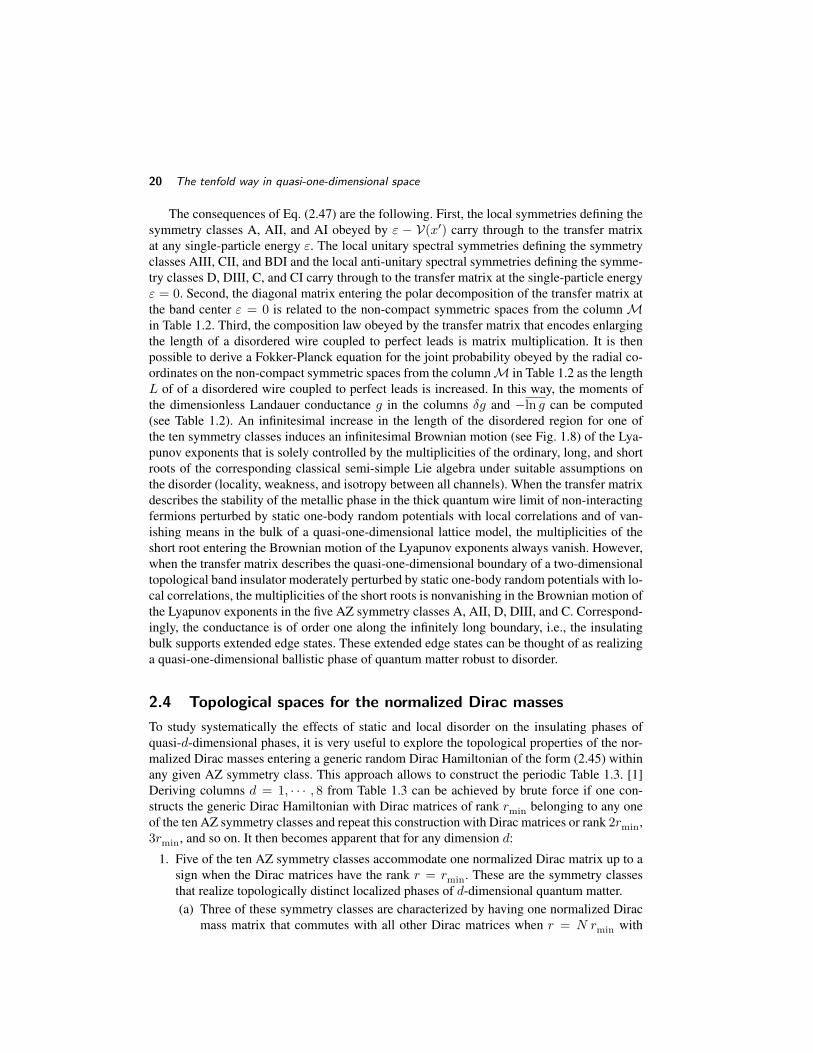


![COMPUTABLE ABELIAN GROUPS - Massey Universityamelniko/survey.pdf · COMPUTABLE ABELIAN GROUPS 5 standard references for pure abelian group theory are Fuchs [44, 45] and Kaplansky](https://static.documents.pub/doc/80x56/5f0639277e708231d416ea0e/computable-abelian-groups-massey-university-amelnikosurveypdf-computable-abelian.jpg)