Page 1
Lehigh UniversityLehigh Preserve
Theses and Dissertations
2011
Fracture Analysis Using Enriched Finite Elementsfor Three-Dimensional Welded StructuresZhiye LILehigh University
Follow this and additional works at: http://preserve.lehigh.edu/etd
This Thesis is brought to you for free and open access by Lehigh Preserve. It has been accepted for inclusion in Theses and Dissertations by anauthorized administrator of Lehigh Preserve. For more information, please contact [email protected] .
Recommended CitationLI, Zhiye, "Fracture Analysis Using Enriched Finite Elements for Three-Dimensional Welded Structures" (2011). Theses andDissertations. Paper 1202.
Page 2
FRACTURE ANALYSIS USING ENRICHED
FINITE ELEMENTS for THREE-DIMENSIONAL
WELDED STRUCTURES
by
Zhiye Li
Presented to the Graduate and Research Committee
of Lehigh University
in Candidacy for the Degree of
Master of Science
in
Mechanical Engineering
Lehigh University
2011
Page 3
ii
Approved and recommended for acceptance as a dissertation in partial
fulfillment of the requirements for the Degree of Master of Science.
___________________
Date
________________________
Thesis Advisor
________________________
Chairperson of Department
Page 4
iii
Acknowledgments
I gratefully thank my advisor Prof. Herman F. Nied for his constructive
comments on my research and this thesis. Without his support and knowledge, it
would be hard to complete this thesis.
Also, I express my love to my parents.
Page 5
iv
Table of Contents
Table of Contents iv
List of Figures vi
List of tables xi
Abstract 1
Chapter 1. Introduction 3
1.1 Finite element analysis of crack problems 3
1.2 Welding simulation 8
1.3 Finite element analysis of 3D welding/ fracture Problem 11
Chapter 2. Numerical Analysis 16
2.1 Numerical Method 16
2.2 Welding Geometry 21
2.3 Mesh Generation 24
2.4 HYPERMESH®/SYSWELD® Interface 28
Chapter 3.Fusion Welding Simulation 31
3.1 Material Properties and Fusion Welding Simulation 31
3.2 Initial Clamping Condition 35
3.3 Heat Source Modeling 36
3.4 Heat Transfer Modeling 40
3.5 Thermal Analysis 42
Page 6
v
3.6 Mechanical Analysis 45
Chapter 4.Fracture Mechanics Analysis 46
4.1 Finite Element code FRAC_3D 46
4.2 SYSWELD/FRAC3D Interface 51
4.3 Superposition Results 54
Chapter 5.Conclusions and Furture Work 57
5.1 Finite element analysis of crack problems 57
5.2 Future Works 85
References 87
Appendix 91
VITA 117
Page 7
vi
List of Figures
Figure 1.1 Running FRAC3D 4
Figure 1.2 Graphical User Interface FCPAS based on Frac3D and ANSYS 5
Figure 2.1 Schematic flow chart for the file transfer process 17
Figure 2.2 geometry of Longitudinal-Bead-Weld Notch-Bend test specimen 21
Figure 2.3 Longitudinal-Bead-Weld Notch-Bend test specimen in Fracture analysis 22
Figure 2.4 1/4 welding bead model 23
Figure 2.5 cross section of 1/4 welding bead model 23
Figure 2.6 3D mesh generation of Longitudinal-Bead-Weld Notch-Bend model 24
Figure 2.7 2D mesh and 1D mesh of Longitudinal-Bead-Weld Notch-Bend model 25
Figure 2.8 2D mesh and 1D mesh of Longitudinal-Bead-Weld Notch-Bend model 25
Figure 2.9 Cross section 26
Figure 2.10 (a) Hex20, 3D (2nd order)quadrilateral hexahedra element with 20 nodes in
HYPERMESH.(b)Quad8, 2D (2nd order)quadrilateral elements with 8 nodes ordered
in HYPERMESH 28
Figure 2.11 Element definition and nodal number order in SYSWELD 29
Figure 3.1 Trajectory line and reference line for fusion welding 34
Figure 3.2 Initial boundary condition 35
Figure 3.3 Double ellipsoid source and display of possible trajectories 36
Figure 3.4 Weld pool 38
Figure 3.5 Calibrating heat sources 38
Page 8
vii
Figure 3.6 Moving heat source 42
Figure 3.7 (a) Temperature distribution of plate-bead. (b) Temperature distribution of
z-direction symmetry plane 43
Figure 4.1 20-Node three-dimensional enriched crack tip element 47
Figure 4.2 General flow of FRAC_3D analysis 49
Figure 4.3 Surface Loads Pressures format, face 1: (J-I-L-K), face 2: (I-J-N-M), face 3
(J-K-O-N), face 4: K-L-P-O), face 5: (L-I-M-P), face 6 (M-N-O-P) 52
Figure 5.1 Model description 57
Figure 5.2 Temperature distribution after fusion welding (time=2000second) 59
Figure 5.3 Residual stress distribution after fusion welding (time=2000second) 59
Figure 5.4 Temperature distributions during welding process. (1) t=5; (2) t=10; (3) t=20;
(4) t=30; (5) t=40; (6) t=50. 60
Figure 5.5 Temperature distributions after welding(time=50s) 61
Figure 5.6 configurations. (1) of the whole welding plate (2) Residual stress
in crack surface after fusion welding (3) Cross view of in plane of crack
surface (4) along the crack front. 61
Figure 5.7 Von Mises stress distributions during welding process. (1) t=5; (2) t=10; (3)
t=20; (4) t=30; (5) t=40; (6) t=50. 62
Figure 5.8 Von Mises stress distributions during cooling process. (1) t=75; (2) t=257; (3)
t=542; (4) t=1183; (5) t=1788; (6) t=2000. 63
Page 9
viii
Figure 5.9 Residual stress σ33 distributions during welding process. (1) t=5; (2) t=10;
(3) t=20; (4) t=30; (5) t=40; (6) t=50. 64
Figure 5.10 Residual stress σ33 distributions during cooling process. (1) t=75; (2)
t=257; (3) t=542; (4) t=1183; (5) t=1788; (6) t=2000. 65
Figure 5.11 Displacements Magnitude after crack 66
Figure 5.12 Total stress configurations in direction of zz axial 66
Figure 5.13 Stress Intensity factor (Mpa/ ) 67
Figure 5.14 Temperature distributions during welding process. (1) t=5; (2) t=10; (3)
t=20; (4) t=30; (5) t=40; (6) t=50. 68
Figure 5.15 Temperature distributions after welding(time=50s) 69
Figure 5.16 Residual stresses distribution after fusion welding for finer mesh case 69
Figure 5.17 Von Mises stress distributions during welding process. (1) t=5; (2) t=10; (3)
t=20; (4) t=30; (5) t=40; (6) t=50. 70
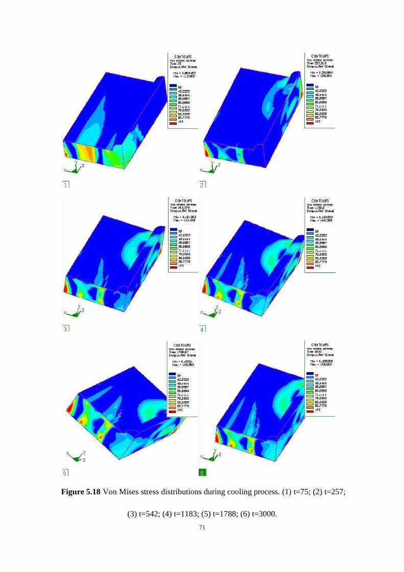
Figure 5.18 Von Mises stress distributions during cooling process. (1) t=75; (2) t=257;
(3) t=542; (4) t=1183; (5) t=1788; (6) t=3000. 71
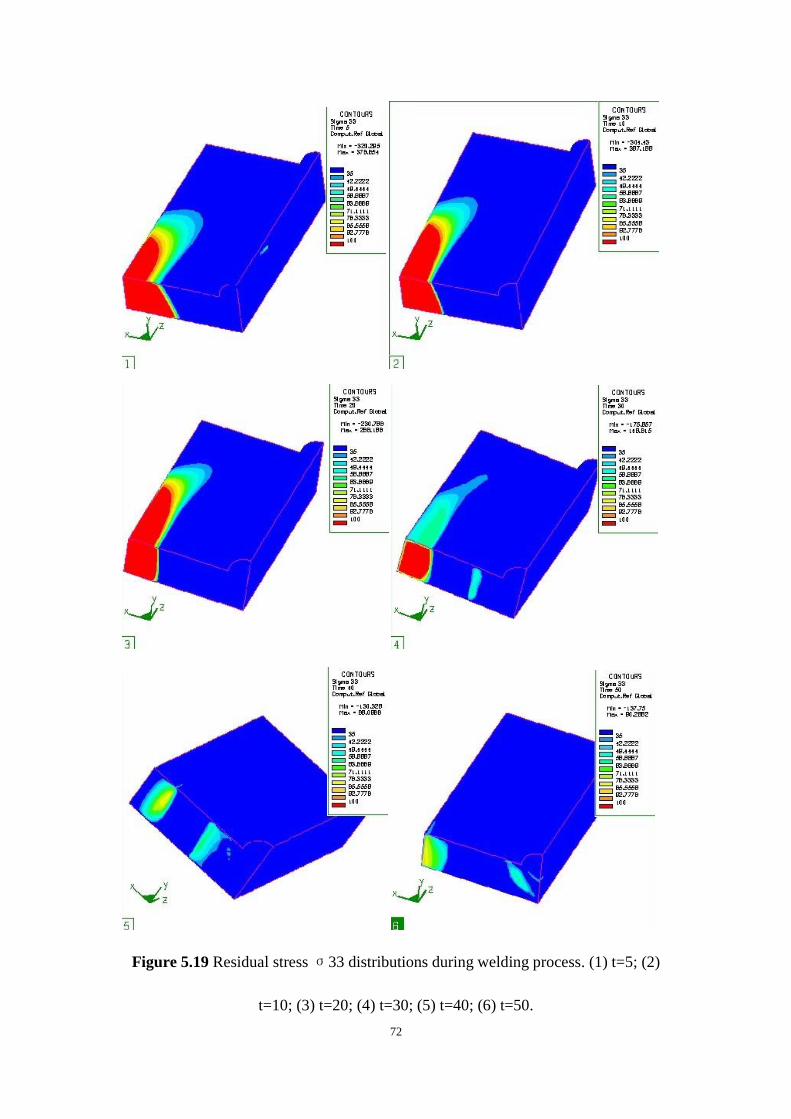
Figure 5.19 Residual stress σ33 distributions during welding process. (1) t=5; (2) t=10;
(3) t=20; (4) t=30; (5) t=40; (6) t=50. 72
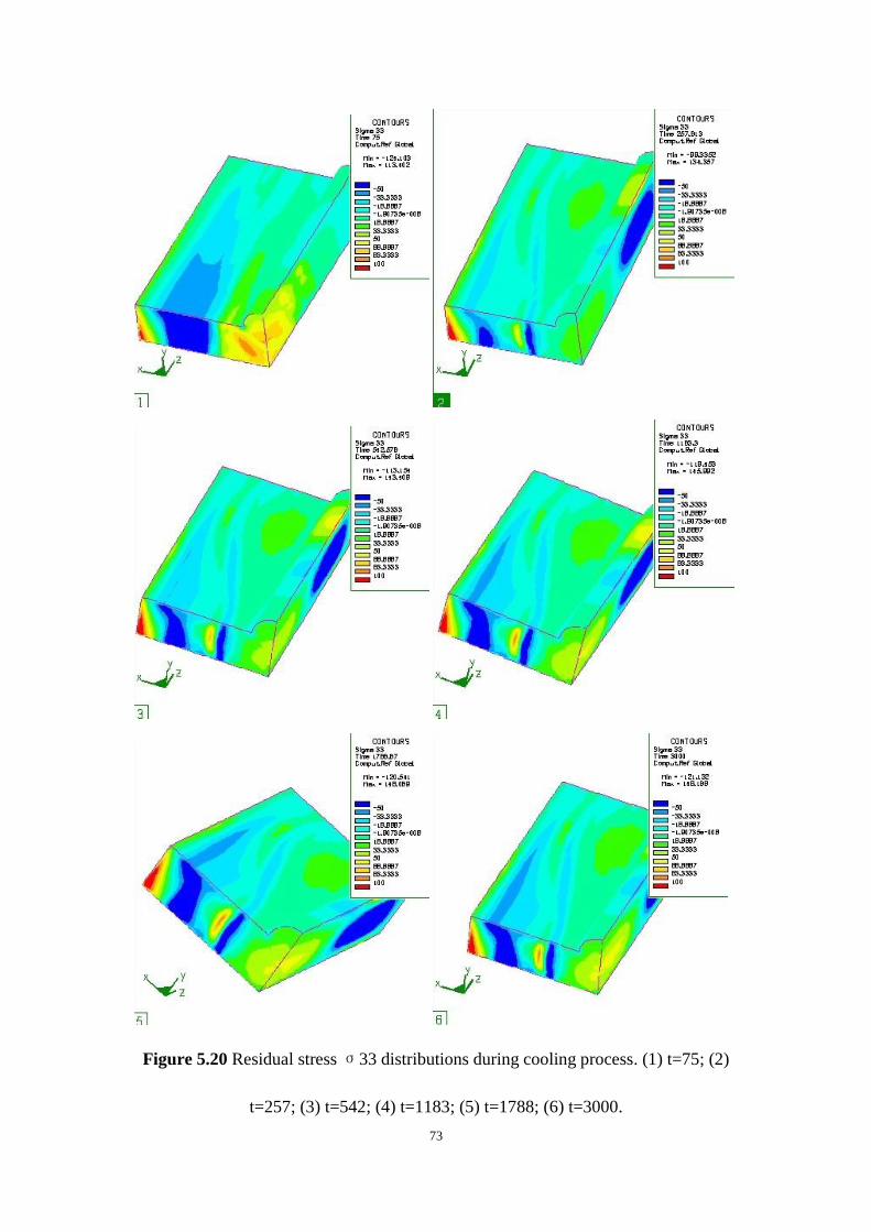
Figure 5.20 Residual stress σ33 distributions during cooling process. (1) t=75; (2)
t=257; (3) t=542; (4) t=1183; (5) t=1788; (6) t=3000. 73
Page 10
ix
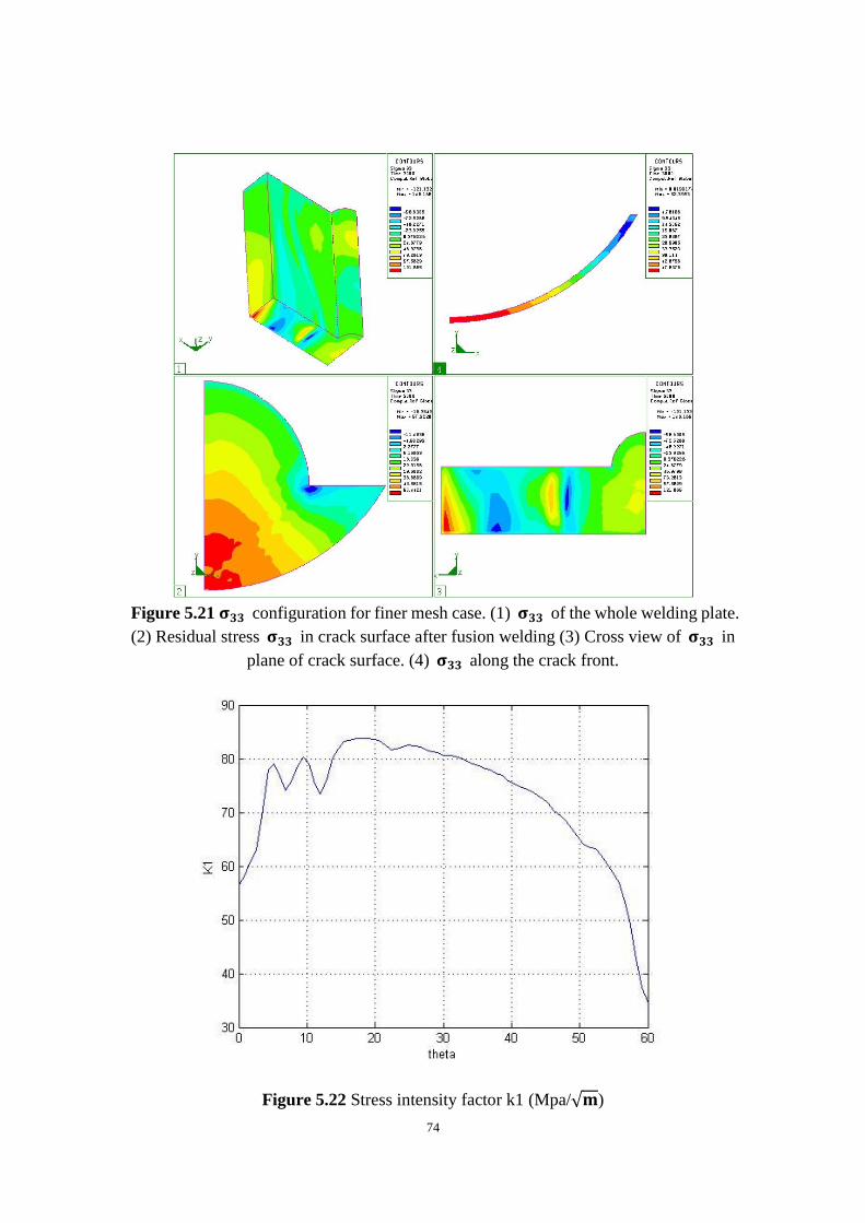
Figure 5.21 configuration for finer mesh case. (1) of the whole welding plate.
(2) Residual stress in crack surface after fusion welding (3) Cross view of in
plane of crack surface. (4) along the crack front. 74
Figure 5.22 Stress intensity factor k1 (Mpa/ ) 74
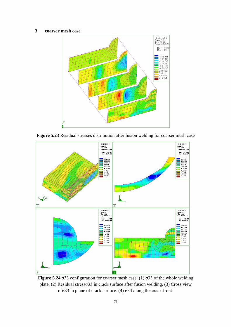
Figure 5.23 Residual stresses distribution after fusion welding for coarser mesh case
75
Figure 5.24 σ33 configuration for coarser mesh case. (1) σ33 of the whole welding plate.
(2) Residual stressσ33 in crack surface after fusion welding. (3) Cross view ofσ33 in
plane of crack surface. (4) σ33 along the crack front. 75
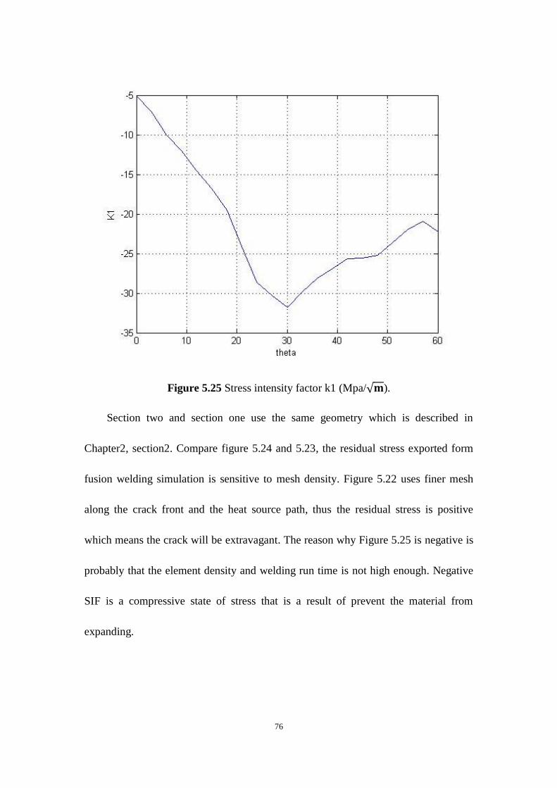
Figure 5.25 Stress intensity factor k1 (Mpa/ ). 76
Figure 5. 26 Temperature distributions during welding process. (1) t=5; (2) t=10; (3)
t=20; (4) t=30; (5) t=40; (6) t=50. 77
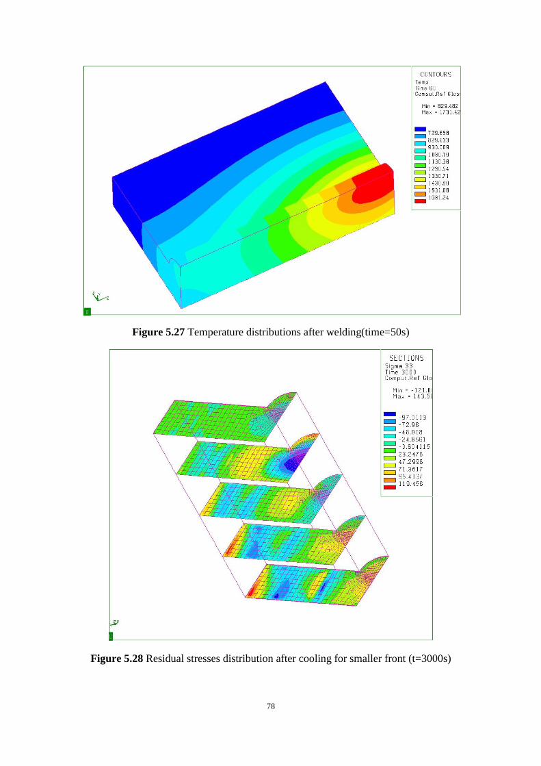
Figure 5.27 Temperature distributions after welding(time=50s) 78
Figure 5.28 Residual stresses distribution after cooling for smaller front (t=3000s) 78
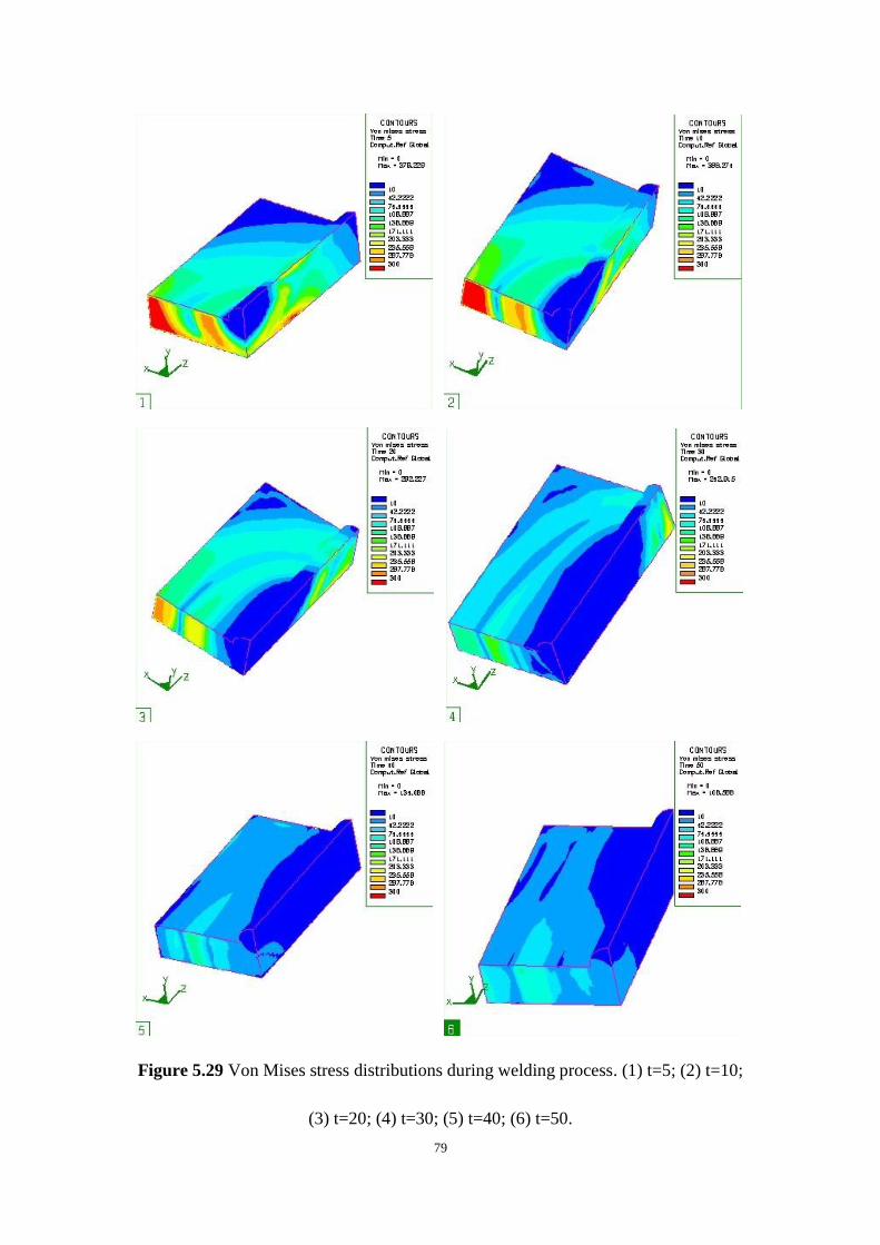
Figure 5.29 Von Mises stress distributions during welding process. (1) t=5; (2) t=10; (3)
t=20; (4) t=30; (5) t=40; (6) t=50. 79
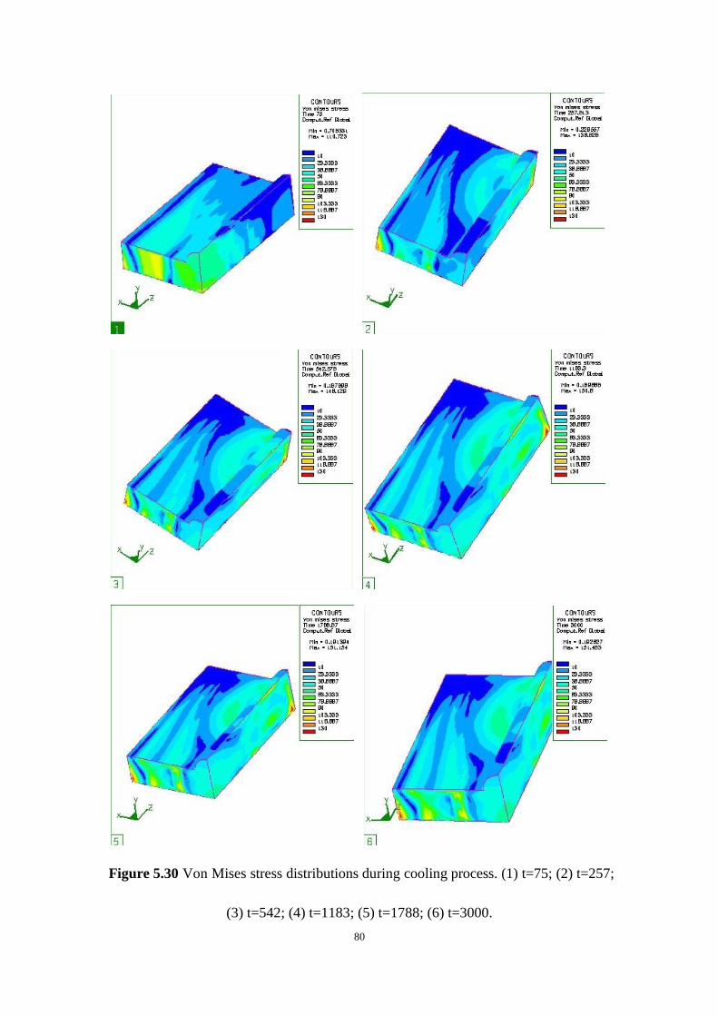
Figure 5.30 Von Mises stress distributions during cooling process. (1) t=75; (2) t=257;
(3) t=542; (4) t=1183; (5) t=1788; (6) t=3000. 80
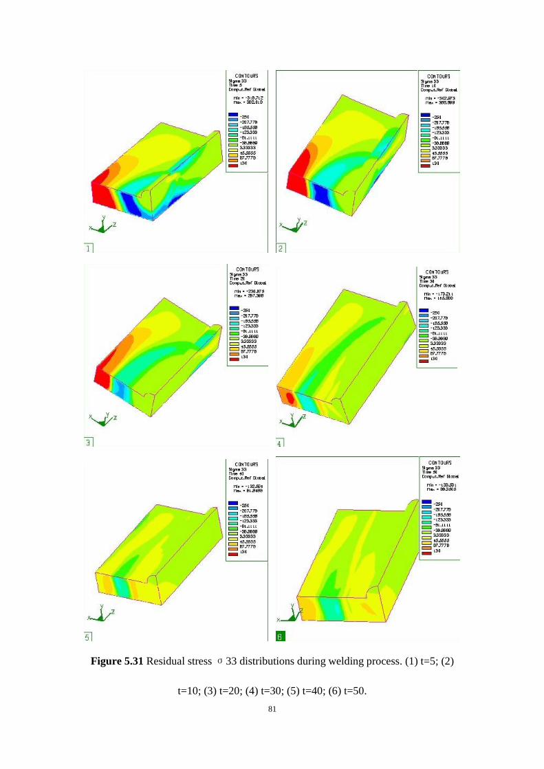
Figure 5.31 Residual stress σ33 distributions during welding process. (1) t=5; (2) t=10;
(3) t=20; (4) t=30; (5) t=40; (6) t=50. 81
Page 11
x
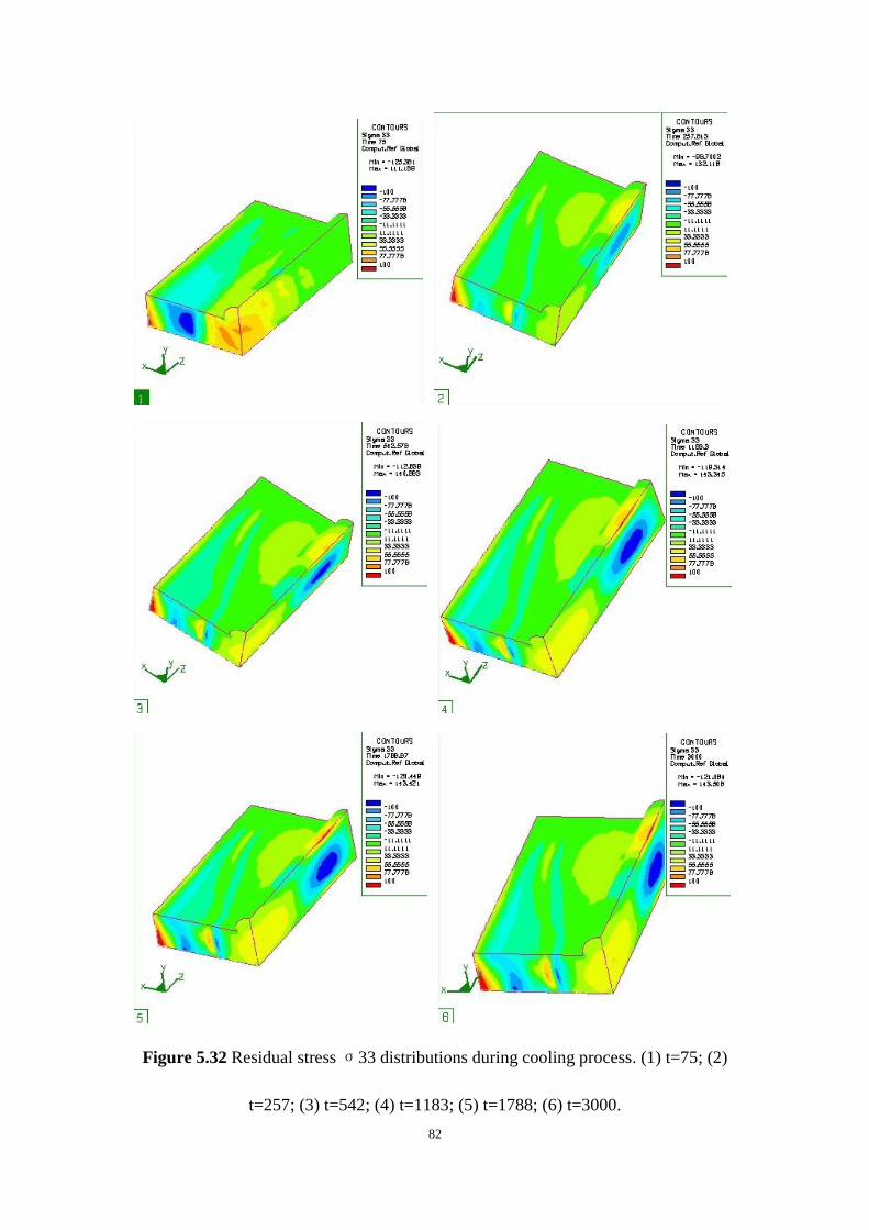
Figure 5.32 Residual stress σ33 distributions during cooling process. (1) t=75; (2)
t=257; (3) t=542; (4) t=1183; (5) t=1788; (6) t=3000. 82
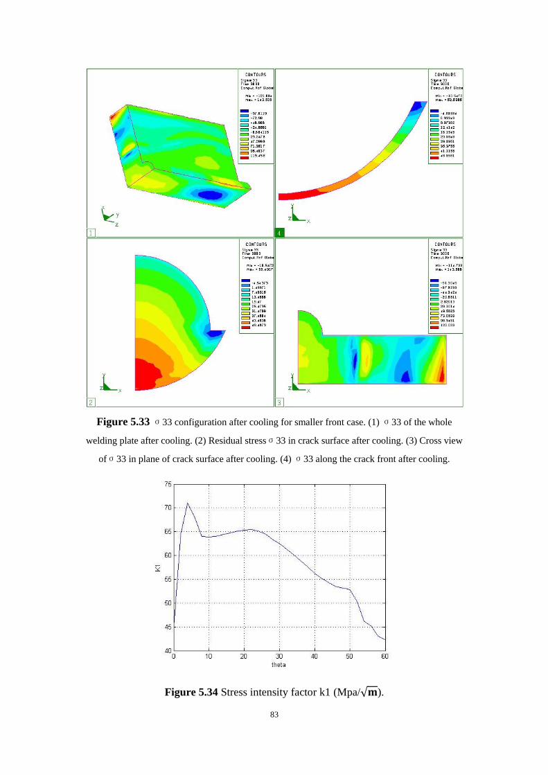
Figure 5.33 σ33 configuration after cooling for smaller front case. (1) σ33 of the
whole welding plate after cooling. (2) Residual stressσ33 in crack surface after
cooling. (3) Cross view ofσ33 in plane of crack surface after cooling. (4) σ33 along
the crack front after cooling. 83
Figure 5.34 Stress intensity factor k1 (Mpa/ ). 83
Figure 5.35 Total stress configurations in direction of zz axial 84
Figure 5.36 Current model and model for future work. 85
Page 12
xi
List of tables
Table3.1 Chemical composition of the consumable materials (in wt%) 32
Table3.2 Typical mechanical properties 32
Page 13
1
Abstract
The objective of this investigation is to evaluate the effect of residual stresses
that arise during welding processes, on localized fracture behavior. The primary
fracture parameters of interest are the Stress Intensity Factors (SIFs) associated with
cracks that develop around the welded area. The simulation of the welding process is
accomplished through the finite element code SYSWELD® and the computation of
fracture behavior uses a finite element user-defined enriched crack tip element code,
FRAC3D, developed at Lehigh University. In this study, quadratic 3D finite element
models which are generated in HYPERMESH®, are first introduced into
SYSWELD® to perform the thermo-mechanical transient analysis needed to predict
the welding residual stresses, global stresses, stain and displacement. Residual
stresses form the welding simulation and the original quadratic 3D finite element
HYPERMESH® model are combined, modified and transferred into the
ANSYS/FRAC3D code to obtain the final Stress Intensity Factor (SIF) for 3D cracks,
and the stresses, strains and displacements in the cracked configuration. In order to
verify the accuracy of the welding simulation residual stress, different mesh densities
were examined in detail. In addition, different welding model meshes were applied to
test the sensitivity of the SIF results to different meshes and geometries. Finally,
refined weld/crack models with a progression of crack shapes that follow the contours
of the highest stresses around the weld zone were generated to simulate the behavior
Page 14
2
of a crack emerging from a weld defect The effect that different welding parameters
have on the fracture parameters represent an important result from this study.
Page 15
3
Chapter 1. Introduction
1.1 Finite element analysis of crack problems
Finite element analysis of three-dimensional fracture problems based on linear
elastic fracture mechanics is an important tool for design analysis in industry.
Meaningful 3-D fracture computations should include such quantities as mixed mode
stress intensity factors, strain energy release rate, and phase angles to be considered as
an appropriate engineer tool with broad applications. Fracture analysis of structures
fabricated using welding also require careful consideration of the welding residual
stresses that often result in localized cracking in the neighborhood of the weld. Such a
fracture analysis requires a systematic technique to link the results from the welding
simulation with secondary computations needed to extract the relevant fracture
parameters, e.g. stress intensity factors. One problem when using the finite element
methodology to analyze crack problems is the difficulty in adequately capturing the
mathematical singularity that occurs at the hypothetical crack tip in linear elastic
bodies. The usual polynomial based elements available in most commercially
available finite element codes converge very slowly to a suitably accurate solution
when the finite element model contains a sharp crack that does not incorporate the
correct asymptotic solution with the appropriate √ singular stress terms.
Enriched finite elements are very convenient for representation of singularities in
Page 16
4
fracture analysis. In this study, a specialized finite element program [1], which uses
enriched crack tip elements, developed at Lehigh University, is utilized to perform the
fracture analysis for this research.
In 2002, Ayhan and Nied[2] implemented asymptotic terms into enriched
elements for six different types of 3-D elements and developed an efficient finite
element code, which could perform fracture mechanics analysis for three dimensional
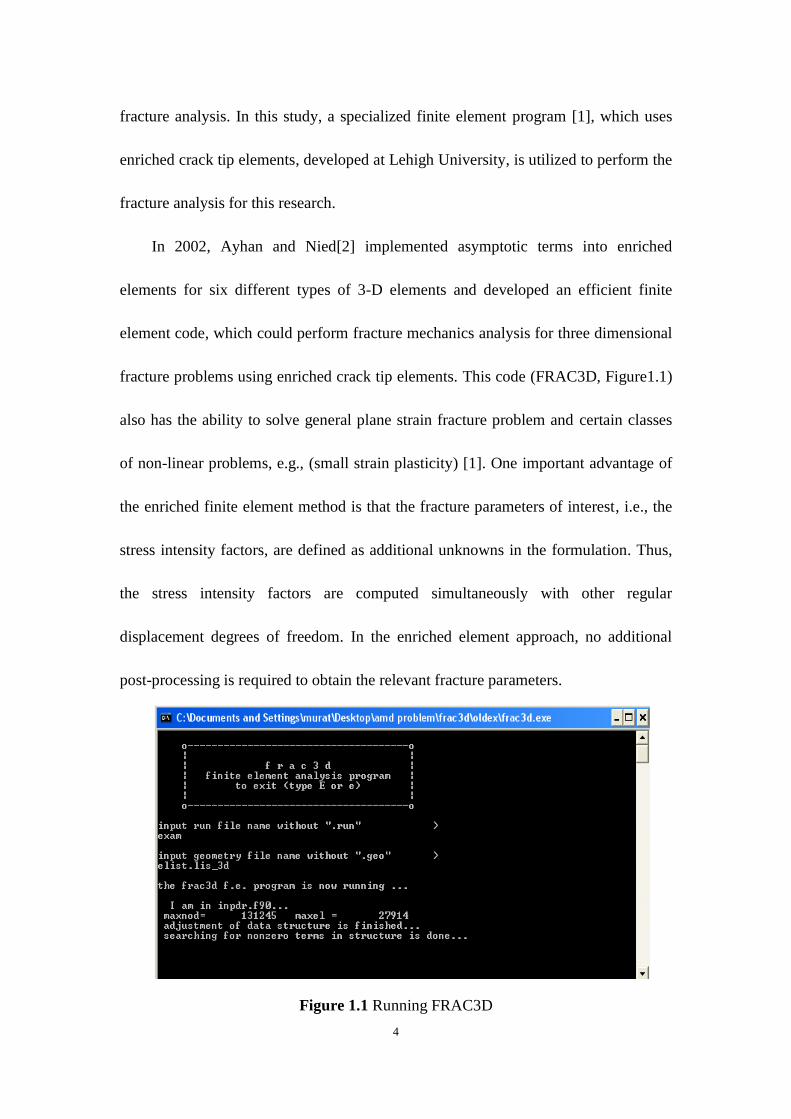
fracture problems using enriched crack tip elements. This code (FRAC3D, Figure1.1)
also has the ability to solve general plane strain fracture problem and certain classes
of non-linear problems, e.g., (small strain plasticity) [1]. One important advantage of
the enriched finite element method is that the fracture parameters of interest, i.e., the
stress intensity factors, are defined as additional unknowns in the formulation. Thus,
the stress intensity factors are computed simultaneously with other regular
displacement degrees of freedom. In the enriched element approach, no additional
post-processing is required to obtain the relevant fracture parameters.
Figure 1.1 Running FRAC3D
Page 17
5
One aspect of the enriched element formulation is the need for transition
elements to rigorously satisfy displacement compatibility. Displacement compatibility
is satisfied exactly on all element surfaces between the enriched crack tip elements
and the surrounding isoperimetric finite elements in this methodology. The
formulation for 3-D interfacial crack problems was updated in FRAC3D by Ayhan,
Kaya and Nied[3]. Further development of this research code continues, e.g., in 2010,
Ayhan developed a Graphical User Interface FCPAS (Figure 1.2) based on Frac3D
and ANSYS.
Figure 1.2 Graphical User Interface FCPAS based on Frac3D and ANSYS
Most commercially available finite element codes have some capacity for
fracture analysis. For example, ANSYS [4] can be used to compute stress intensity
factors using the virtual crack extension technique. However, this requires the
Page 18
6
generation of a specialized “tunnel” crack tip mesh that completely surrounds the
crack front, which greatly complicates the generation of a mesh for a general 3-D
problem. The main benefit of using FRAC3D in this study, is that the finite element
meshes used for fracture analyses of the welded geometry do not require specialized
crack tip meshes, and thus automatic meshing from HYPERMESH® can be routinely
used to a generate mesh for the cracked structure.
In the paper by Ayhan and Nied [1], it was demonstrated that even for coarse
finite element meshes, the direct calculation of the stress intensity factors using
enriched elements, results in rapid convergence to the correct stress intensity factor
solution. Currently, enrichment capabilities of FRAC3D include asymptotic crack tip
elements for: interface cracks, anisotropic materials, poroelastic materials, dynamic
loading and crack surface contact.
However, fracture analysis for welded structures is somewhat different than the
type of fracture problems that are routinely addressed in most engineering fracture
problems. First, the highly nonlinear nature of the welding physics requires a separate
type of finite element formulation to take into account the melting and resolidification
that occurs during welding. The welding simulation can be completely separate from
the fracture analysis. However, the residual stresses are an important driving force (in
conjunction with additional external loads) for subsequent crack growth when a
welded structure is in actual use. This combination of welding simulation and fracture
Page 19
7
analysis is of considerable importance, since weld joints are considered to be the
portion of the structure most susceptible to cracking.
Page 20
8
1.2 Welding simulation
Cracking behavior is strongly influenced by the residual stresses which arise
during the fusion welding process. Computation of heat transfer and welding induced
residual stress invariably involves a complex nonlinear numerical simulation of the
fusion weld process, starting with the heat source description, and its moving path
definition. Since the thermo-mechanical properties depend on temperature in a highly
nonlinear manner, analysis of welding requires highly computationally intensive
simulation. In order to meet this need, specialized finite element codes have been
developed that can model and simulate a variety of fusion welding processes. In
addition, many of the larger commercial finite element packages, e.g., ANSYS,
ABAQUS, can be made to simulate welding processes by using appropriate
user-defined moving heat sources and nonlinear material property models.
SYSWELD [5] is a specialized commercial code specifically designed to handle
complex welding simulations and contains built in welding heat source models and
the necessary material property behavior to accurately simulate a wide variety of
welding behavior.
The paper of Suraj Joshi, Cumali Semetay, John WH Price and Herman F. Nied
[6] presents the simulation of welding-induced residual stresses in a CHS T-Joint,
which would form the first of the four lacings welded on to the main chord of a
typical mining dragline cluster. In this paper, computed temperature distributions
during fusion welding and relevant welding distortion for CHS T-joint are presented.
Page 21
9
The paper compares numerically generated residual stresses during the welding
process in a single weld pass, and the observation that residual stresses in the fused
area at some points can be higher than the uniaxial yield stress. The moving heat
source defined in these fusion welding simulations, utilized double-ellipsoid power
density distribution functions, which adequately describe the heat transfer behavior
for various metal arc welding processes.
After the transient temperature distribution during welding has been determined,
the residual stresses can be calculated by performing a nonlinear thermal stress
analysis of the structure as the weld cools from above its melting temperature, down
to the normal environmental temperature. The residual stress components in the weld
region often can become greater than the temperature dependent uniaxial yield
strength of the filler metal as the welded part cools. This is due to localized triaxial
constraint that causes relatively high hydrostatic stresses during cooling solidification
in the neighborhood of the weld. Long longitudinal welds are generally subjected to
longitudinal tensile residual stress approximately equal to the metal‟s uniform axial
yield stress, unless post-weld heat treatment or some other residual stress reduction
treatment is performed. In order to compute residual stress correctly, the stresses that
result from solid phase transformation also should be considered in the residual stress
computation.
Solid phase transformations during cooling are known to cause local material
dilatation and contribute to additional strains similar to thermal strains. [6] This effect
Page 22
10
can be substantial and can even reverse the sign of the residual stresses in determined
solely from a thermo-mechanical simulation.
Page 23
11
1.3 Finite element analysis of 3D welding/ fracture
Problem
The fracture behavior of welded structures is of considerable importance, since
fusion welding is the most commonly used technique for joining metal structures.
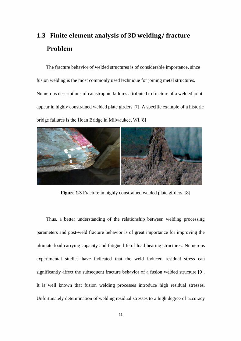
Numerous descriptions of catastrophic failures attributed to fracture of a welded joint
appear in highly constrained welded plate girders [7]. A specific example of a historic
bridge failures is the Hoan Bridge in Milwaukee, WI.[8]
Figure 1.3 Fracture in highly constrained welded plate girders. [8]
Thus, a better understanding of the relationship between welding processing
parameters and post-weld fracture behavior is of great importance for improving the
ultimate load carrying capacity and fatigue life of load bearing structures. Numerous
experimental studies have indicated that the weld induced residual stress can
significantly affect the subsequent fracture behavior of a fusion welded structure [9].
It is well known that fusion welding processes introduce high residual stresses.
Unfortunately determination of welding residual stresses to a high degree of accuracy
Page 24
12
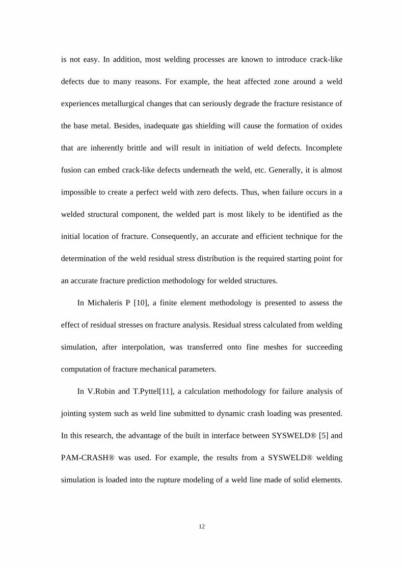
is not easy. In addition, most welding processes are known to introduce crack-like
defects due to many reasons. For example, the heat affected zone around a weld
experiences metallurgical changes that can seriously degrade the fracture resistance of
the base metal. Besides, inadequate gas shielding will cause the formation of oxides
that are inherently brittle and will result in initiation of weld defects. Incomplete
fusion can embed crack-like defects underneath the weld, etc. Generally, it is almost
impossible to create a perfect weld with zero defects. Thus, when failure occurs in a
welded structural component, the welded part is most likely to be identified as the
initial location of fracture. Consequently, an accurate and efficient technique for the
determination of the weld residual stress distribution is the required starting point for
an accurate fracture prediction methodology for welded structures.
In Michaleris P [10], a finite element methodology is presented to assess the
effect of residual stresses on fracture analysis. Residual stress calculated from welding
simulation, after interpolation, was transferred onto fine meshes for succeeding
computation of fracture mechanical parameters.
In V.Robin and T.Pyttel[11], a calculation methodology for failure analysis of
jointing system such as weld line submitted to dynamic crash loading was presented.
In this research, the advantage of the built in interface between SYSWELD® [5] and
PAM-CRASH® was used. For example, the results from a SYSWELD® welding
simulation is loaded into the rupture modeling of a weld line made of solid elements.
Page 25
13
The damage parameters are identified through an inverse method based on
comparisons between numerical and experimental results.
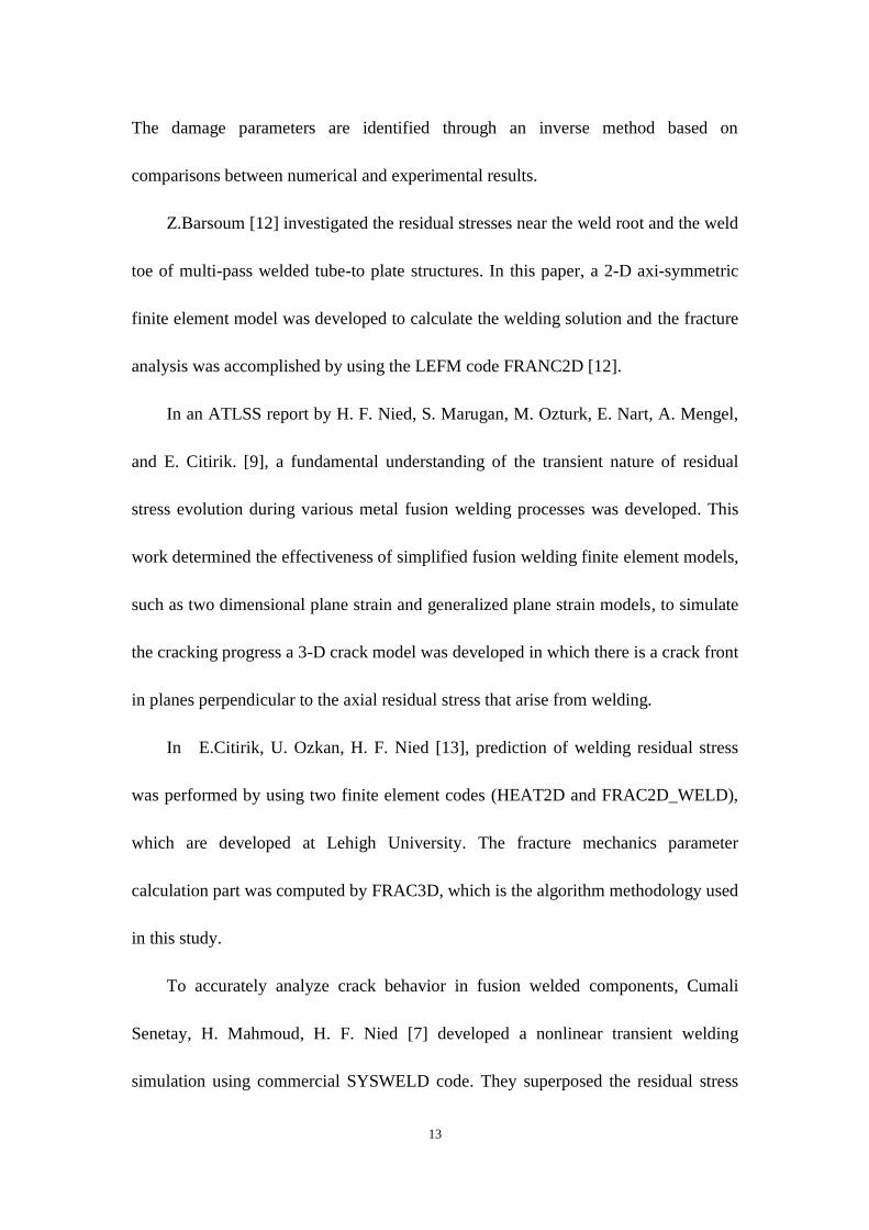
Z.Barsoum [12] investigated the residual stresses near the weld root and the weld
toe of multi-pass welded tube-to plate structures. In this paper, a 2-D axi-symmetric
finite element model was developed to calculate the welding solution and the fracture
analysis was accomplished by using the LEFM code FRANC2D [12].
In an ATLSS report by H. F. Nied, S. Marugan, M. Ozturk, E. Nart, A. Mengel,
and E. Citirik. [9], a fundamental understanding of the transient nature of residual
stress evolution during various metal fusion welding processes was developed. This
work determined the effectiveness of simplified fusion welding finite element models,
such as two dimensional plane strain and generalized plane strain models, to simulate
the cracking progress a 3-D crack model was developed in which there is a crack front
in planes perpendicular to the axial residual stress that arise from welding.
In E.Citirik, U. Ozkan, H. F. Nied [13], prediction of welding residual stress
was performed by using two finite element codes (HEAT2D and FRAC2D_WELD),
which are developed at Lehigh University. The fracture mechanics parameter
calculation part was computed by FRAC3D, which is the algorithm methodology used
in this study.
To accurately analyze crack behavior in fusion welded components, Cumali
Senetay, H. Mahmoud, H. F. Nied [7] developed a nonlinear transient welding
simulation using commercial SYSWELD code. They superposed the residual stress
Page 26
14
and external load from an ABAQUS finite element simulation and used these results
to perform a fracture analysis.
The paper by Labeas, Tsirkas, Diamantakos, and Kermanidis [14] introduces an
effective method to study the effect of residual stresses due to laser welding on the
Stress Intensity Factors (SIFs) of cracks developing nearby the welded area. The
simulation of the welding process and the calculation of SIFs on the cracked structure
are performed using an explicit and an implicit Finite Element code, respectively. The
developed residual stresses due to the welding of two flat plates by laser welding are
calculated first, using a thermo-mechanical transient analysis. Subsequently, a linear
elastic analysis is applied for the calculation of SIFs at the crack tips. For the entire
finite element calculation, linear solid elements „SOLID45‟ in the ANSYS code are
used. SOLID45 is a brick element and is defined by eight nodes, having three
displacement degrees of freedom at each element node. The calculated results of the
welding simulation are verified by comparing the computed angular distortions to the
corresponding experimental values. The verification of the important fracture
mechanics parameter SIF is performed through comparisons between computed and
experimental crack opening displacement (COD) values.
In this study the residual stresses that arise during the weld process are a function
of the welding parameters, e.g., material phase, temperature, displacement, etc. Thus,
the influence of different weld parameters on the fracture behavior -is an important
result in this study.
Page 27
15
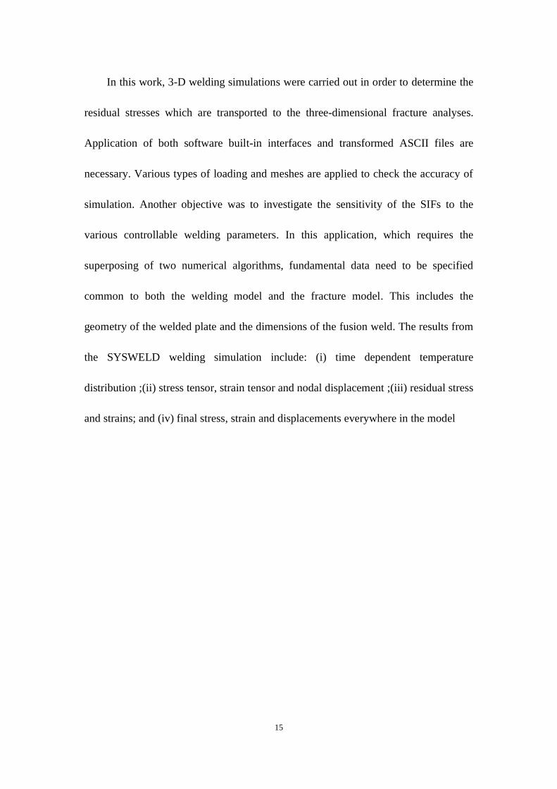
In this work, 3-D welding simulations were carried out in order to determine the
residual stresses which are transported to the three-dimensional fracture analyses.
Application of both software built-in interfaces and transformed ASCII files are
necessary. Various types of loading and meshes are applied to check the accuracy of
simulation. Another objective was to investigate the sensitivity of the SIFs to the
various controllable welding parameters. In this application, which requires the
superposing of two numerical algorithms, fundamental data need to be specified
common to both the welding model and the fracture model. This includes the
geometry of the welded plate and the dimensions of the fusion weld. The results from
the SYSWELD welding simulation include: (i) time dependent temperature
distribution ;(ii) stress tensor, strain tensor and nodal displacement ;(iii) residual stress
and strains; and (iv) final stress, strain and displacements everywhere in the model
Page 28
16
Chapter 2. Numerical Analysis
2.1 Numerical Method
The focus of this numerical study will be on the thermo-mechanical and fracture
behavior of a long longitudinal bead weld (Figure 2.1). This very common weld
geometry contains important features observed in most weld geometries and
represents a generic baseline for developing a systematic numerical methodology for
analyzing weld fracture behavior.
Generally, two types of numerical analyses (welding simulation and fracture
simulation) are required for the fracture mechanics design of longitudinal-bead weld
Crack test specimens with center crack underneath weld bead. The principle goal of
this study is to investigate the residual stresses that arise during the welding process
and their influence on the fracture behavior. Therefore, determination of the residual
stress field that evolves during the fusion welding process is required prior to
computing stress intensity factors for the cracks that may develop along the crack
front near the weld bead.
Simulation of the fusion welding process was performed using the explicit finite
element code SYSWELD [11]. The residual stress field around the welded area
depends on a detailed heat transfer analysis that is exported to the mechanical phase
Page 29
17
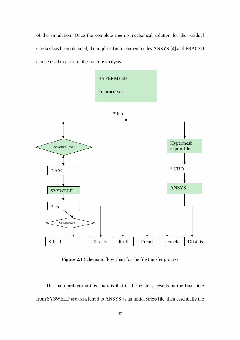
of the simulation. Once the complete thermo-mechanical solution for the residual
stresses has been obtained, the implicit finite element codes ANSYS [4] and FRAC3D
can be used to perform the fracture analysis.
Figure 2.1 Schematic flow chart for the file transfer process
The main problem in this study is that if all the stress results on the final time
from SYSWELD are transferred to ANSYS as an initial stress file, then essentially the
HYPERMESH
Preprocessor
Converter1.exe Hypermesh
export file
*.hm
8
*.ASC *.CBD
SYSWELD ANSYS
*.lis
Converter2.exe
Sflist.lis Elist.lis nlist.lis Ecrack ncrack Dlist.lis
Page 30
18
same results in ANSYS will be obtained as which is obtained in SYSWELD, for the
same geometry parameter, element and node information, and boundary conditions.
However, the SYSWELD model in fact is not completely identical to ANSYS model,
since the SYSWELD model doesn't have a stress-free crack surface, while the
ANSYS model does. Basically in the superposition procedure shown in Figure 2.1,
the residual stresses for the un-cracked configuration are obtained using SYSWELD
and then these stresses are applied as crack surface pressure for the fracture
mechanics calculation. The superposition of the two solutions gives the complete
solution for the final state of stress in the cracked configuration. If the crack is in the
problem before welding occurs, then the heat transfer conditions will simply be
different and at the same time a preexisting flaw may decrease the accuracy of
residual stress results from SYSWELD, i.e., the crack faces should be insulated to
prevent heat from flowing across the crack face surfaces. Admittedly simulation of
model with a crack is an interesting problem in and of itself, but is more
representative of a weld repair problem. On the other hand, the model of interest in
this study represents the case where the crack appears (nucleates) after welding. In
this circumstance, heat transfer is not impeded by any pre-existing crack faces.
The approach that is used in this study relies on a superposition method (figure
2.1), i.e., SYSWELD stress output files are generated to characterize the state of stress
only for the zone where the crack surface will be in the subsequent ANSYS/FRAC3D
model. Thus the residual stress data from SYSWELD is used as an applied crack
Page 31
19
surface pressure on the hypothetical crack surface area. There should be no other
loads acting on the FRAC3D model (refer to a schematic of the superposition
procedure in Figure 2.1) with all other boundary conditions the same. In this approach,
the initial stresses are applied as a pressure on surface element. When this pressure is
applied to a surface, the finite element program will compute the correct consistent
nodal forces that are work equivalent to the pressure distribution, i.e., the FEM
software will determine the proper nodal forces according to pressure information
applied on the crack surface elements. This approach will yield the correct stress
intensity factors in FRAC3D.
After running the FRAC3D program, the initial stresses obtained from
SYSWELD can be added to the FRAC3D results, to determine the complete stress
field, strain field displacement and nodal reaction forces. Clearly, this will result in
cancellation of the stresses on the crack surfaces, providing the correct stresses
throughout the cracked geometry. However, in most instances the full stress field is
not of great interest and only the stress intensity factors are desired. Thus, the actual
superposition of stresses is not generally required.
In this study, the FE model is initially developed using geometry and meshing
tools in the HYPERMESH preprocessor. The finite element entities needed for the
model are transferred to or from the SYSWELD code by way of modified ASCII files
between *.ASC file from SYSWELD and *.CDB HYPERMESH file, which contains
the topology of the model (nodes, elements and sets/groups/components). At the same
Page 32
20
time, the finite element entities of the model are also transferred to ANSYS by way of
transformed ASCII files from *.HM file from HYPERMESH to *.CDB ANSYS file,
which contains the same topology of the model. After simulation of the fusion
welding process in SYSWELD is completed, the computed residual stresses are
exported from the SYSWELD postprocessor as a *.lis file and are imported as
pressure into the ANSYS/FRAC_3D model through a FORTRAN program. The
methodology described, uses the same topology for both of the models required for
the numerical analyses, with the exception of the boundary conditions on the crack
surface. This procedure ensures excellent integration between the two models. One
benefit of this technique, is that it does not require separate meshes for the welding
simulation and the fracture mechanics problem, i.e., both are solved using the same
FE mesh..
Page 33
21
2.2 Welding Geometry
In this study, the modeling and simulation effort focuses on generating solutions
for a simple welded configuration that can easily be tested in experimental facilities.
The test configuration that is modeled in this study is based on the so-called
Longitudinal-Bead-Weld Notch-Bend test specimen [15].
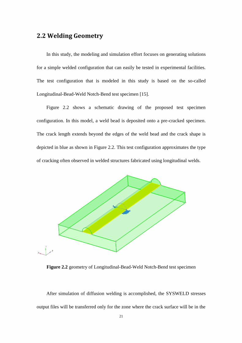
Figure 2.2 shows a schematic drawing of the proposed test specimen
configuration. In this model, a weld bead is deposited onto a pre-cracked specimen.
The crack length extends beyond the edges of the weld bead and the crack shape is
depicted in blue as shown in Figure 2.2. This test configuration approximates the type
of cracking often observed in welded structures fabricated using longitudinal welds.
Figure 2.2 geometry of Longitudinal-Bead-Weld Notch-Bend test specimen
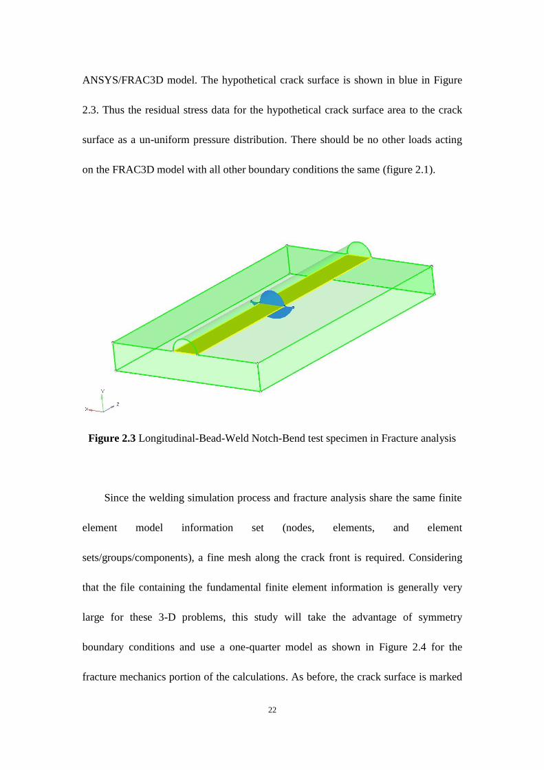
After simulation of diffusion welding is accomplished, the SYSWELD stresses
output files will be transferred only for the zone where the crack surface will be in the
Page 34
22
ANSYS/FRAC3D model. The hypothetical crack surface is shown in blue in Figure
2.3. Thus the residual stress data for the hypothetical crack surface area to the crack
surface as a un-uniform pressure distribution. There should be no other loads acting
on the FRAC3D model with all other boundary conditions the same (figure 2.1).
Figure 2.3 Longitudinal-Bead-Weld Notch-Bend test specimen in Fracture analysis
Since the welding simulation process and fracture analysis share the same finite
element model information set (nodes, elements, and element
sets/groups/components), a fine mesh along the crack front is required. Considering
that the file containing the fundamental finite element information is generally very
large for these 3-D problems, this study will take the advantage of symmetry
boundary conditions and use a one-quarter model as shown in Figure 2.4 for the
fracture mechanics portion of the calculations. As before, the crack surface is marked
Page 35
23
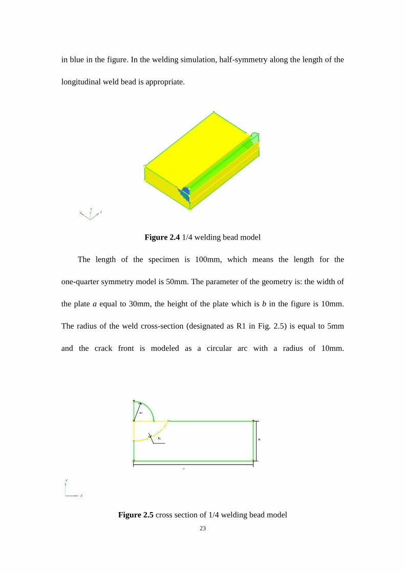
in blue in the figure. In the welding simulation, half-symmetry along the length of the
longitudinal weld bead is appropriate.
Figure 2.4 1/4 welding bead model
The length of the specimen is 100mm, which means the length for the
one-quarter symmetry model is 50mm. The parameter of the geometry is: the width of
the plate a equal to 30mm, the height of the plate which is b in the figure is 10mm.
The radius of the weld cross-section (designated as R1 in Fig. 2.5) is equal to 5mm
and the crack front is modeled as a circular arc with a radius of 10mm.
Figure 2.5 cross section of 1/4 welding bead model
Page 36
24
2.3 Mesh Generation
For volumetric 3-D simulation, three different meshing techniques are employed
to construct the entire mesh for the Longitudinal-Bead-Weld Notch-Bend model using
1)the HYPERMESH mesh generator for SYSWELD solver, 2)WELD ADVISER.
and 3) mesh techniques are applied for ANSYS/FRAC_3D model.
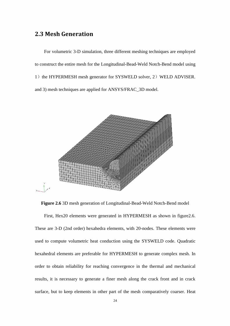
Figure 2.6 3D mesh generation of Longitudinal-Bead-Weld Notch-Bend model
First, Hex20 elements were generated in HYPERMESH as shown in figure2.6.
These are 3-D (2nd order) hexahedra elements, with 20-nodes. These elements were
used to compute volumetric heat conduction using the SYSWELD code. Quadratic
hexahedral elements are preferable for HYPERMESH to generate complex mesh. In
order to obtain reliability for reaching convergence in the thermal and mechanical
results, it is necessary to generate a finer mesh along the crack front and in crack
surface, but to keep elements in other part of the mesh comparatively coarser. Heat
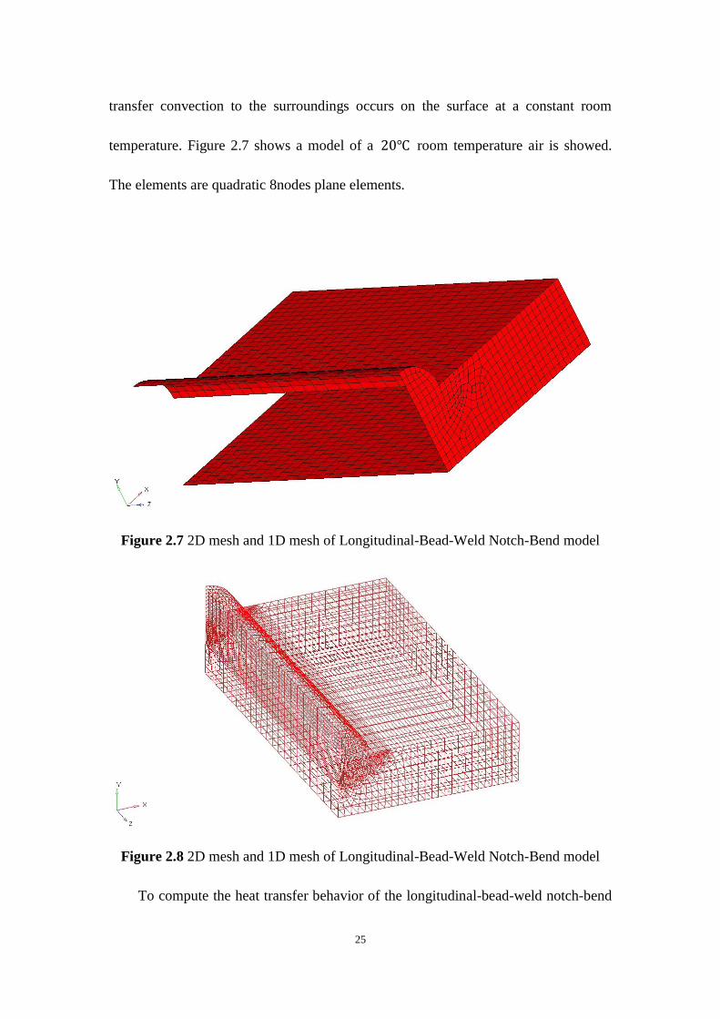
Page 37
25
transfer convection to the surroundings occurs on the surface at a constant room
temperature. Figure 2.7 shows a model of a room temperature air is showed.
The elements are quadratic 8nodes plane elements.
Figure 2.7 2D mesh and 1D mesh of Longitudinal-Bead-Weld Notch-Bend model
Figure 2.8 2D mesh and 1D mesh of Longitudinal-Bead-Weld Notch-Bend model
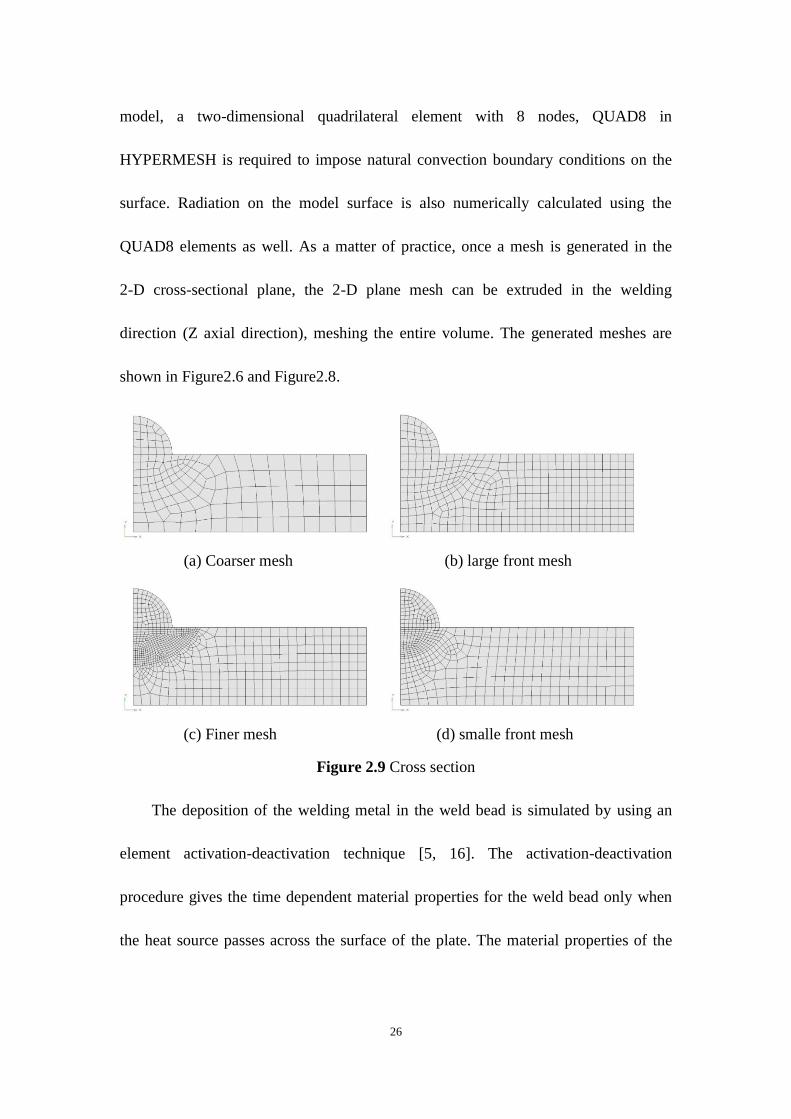
To compute the heat transfer behavior of the longitudinal-bead-weld notch-bend
Page 38
26
model, a two-dimensional quadrilateral element with 8 nodes, QUAD8 in
HYPERMESH is required to impose natural convection boundary conditions on the
surface. Radiation on the model surface is also numerically calculated using the
QUAD8 elements as well. As a matter of practice, once a mesh is generated in the
2-D cross-sectional plane, the 2-D plane mesh can be extruded in the welding
direction (Z axial direction), meshing the entire volume. The generated meshes are
shown in Figure2.6 and Figure2.8.
(a) Coarser mesh (b) large front mesh
(c) Finer mesh (d) smalle front mesh
Figure 2.9 Cross section
The deposition of the welding metal in the weld bead is simulated by using an
element activation-deactivation technique [5, 16]. The activation-deactivation
procedure gives the time dependent material properties for the weld bead only when
the heat source passes across the surface of the plate. The material properties of the
Page 39
27
weld bead and the gap are not given in this study; however, the properties are
activated when the heat source passes through the corresponding nodes.
Since the computational results in SYSWELD and FRAC3D may depend on the
element mesh density, the model described above was meshed using both a large (the
crack front is a part of a circle with a radius of 12mm) front mesh as well as a coarser
mesh and a finer mesh. After comparison of the result e.g. stresses, displacements and
stress intensity factor, a modified model with a progression of crack shapes that
follow the contours of the highest stresses around the weld zone was studied. This
represents a sequence of separate crack configurations
Page 40
28
2.4 HYPERMESH®/SYSWELD® Interface
The Geometry/Meshing module, which is an integral part of SYSWELD
software, is a sophisticated tool for the creation of model geometry and finite element
mesh preprocessor. However, it is more expedient to create a finite element mesh
which can be used in different programs in HYPERMESH. For further possibilities
for the creation of complex geometry and mesh and for computation the same model
in different environment, this study develops a HYPERMESH®/SYSWELD®
Interface. Thus it is possible to convert HYPERMESH standard file to SYSWELD
standard file. Also, it can convert SYSWELD standard file to HYPERMESH standard
file (refer to figure 2.1).
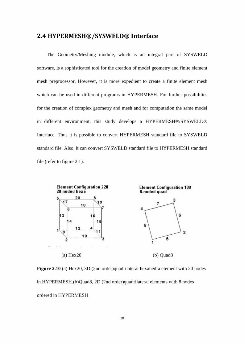
(a) Hex20 (b) Quad8
Figure 2.10 (a) Hex20, 3D (2nd order)quadrilateral hexahedra element with 20 nodes
in HYPERMESH.(b)Quad8, 2D (2nd order)quadrilateral elements with 8 nodes
ordered in HYPERMESH
Page 41
29
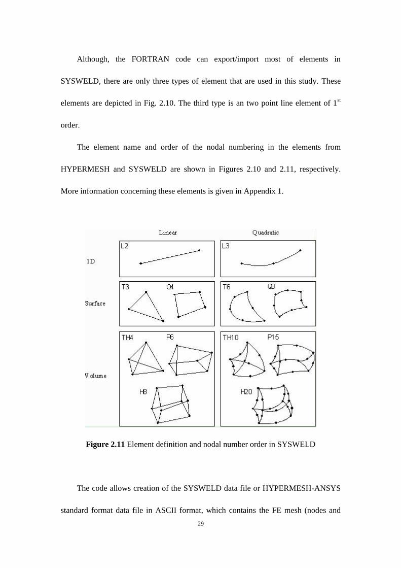
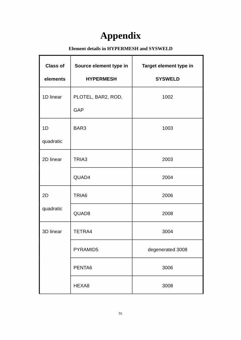
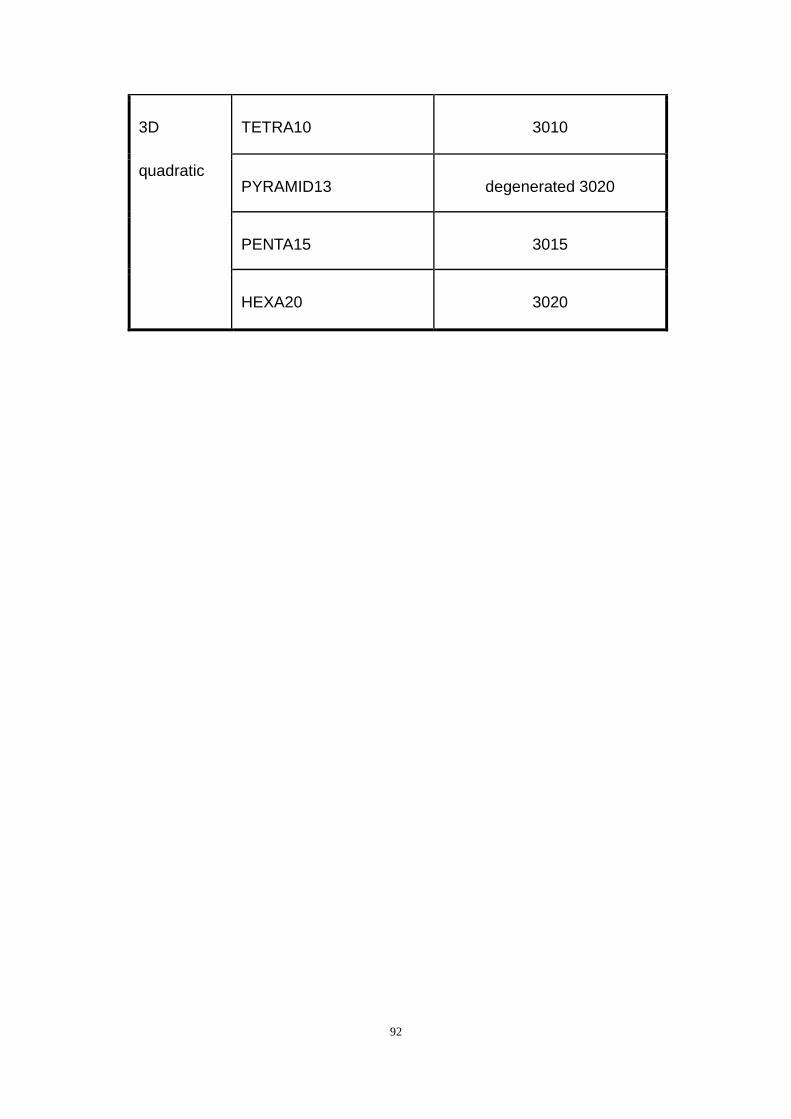
Although, the FORTRAN code can export/import most of elements in
SYSWELD, there are only three types of element that are used in this study. These
elements are depicted in Fig. 2.10. The third type is an two point line element of 1st
order.
The element name and order of the nodal numbering in the elements from
HYPERMESH and SYSWELD are shown in Figures 2.10 and 2.11, respectively.
More information concerning these elements is given in Appendix 1.
Figure 2.11 Element definition and nodal number order in SYSWELD
The code allows creation of the SYSWELD data file or HYPERMESH-ANSYS
standard format data file in ASCII format, which contains the FE mesh (nodes and
Page 42
30
elements) and definition of Groups/Sets. The code does not permit exporting other
pre-processing data, e.g., material properties, constraints, loads, etc.); these are
defined directly in SYSWELD using SYSWELD‟s standard pre-processing
capabilities or advisors or in ANSYS/FRAC_3D using ANSYS preprocessor.
Page 43
31
Chapter 3.Fusion Welding Simulation
3.1 Material Properties and Fusion Welding Simulation
There has been an increasing interest in the effect of fusion welding residual
stresses on mechanical properties, as the design of engineering components has
become less conservative. The effects of residual stresses introduced by fusion
welding are known to play a large role in structural failure mechanisms. Residual
stresses are formed in welded structures primarily as the result of differential
contractions which occur as the weld metal solidifies and cools to the ambient
temperature. These stresses can have important consequences on the performance of
the structure and its fracture behavior.
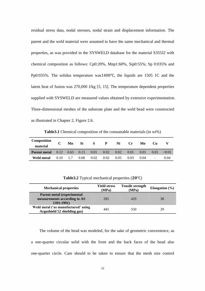
The material used in this study is a low-carbon steel [15].The chemical
composition of the parent material and weld metal are given in Table 3.1. The
dimension of the plate is 100 ; the bead-on-plate welds were
produced along the center line of the plate. The width of the weld beads is 10 mm.
typical mechanical properties of the parent and weld metal are given in Table 3.2. In
the welding simulations, the sample was fully restrained when it is clamped. There
was no pre- or post-weld heat treatment.
The objective of the welding simulation is to perform three-dimensional,
finite-elements modeling of the one-quarter bead-on-plate experiment to export the
Page 44
32
residual stress data, nodal stresses, nodal strain and displacement information. The
parent and the weld material were assumed to have the same mechanical and thermal
properties, as was provided in the SYSWELD database for the material S355J2 with
chemical composition as follows: Cp0:20%, Mnp1:60%, Sip0:55%; Sp 0:035% and
Pp0:035%. The solidus temperature was , the liquids are 1505 1C and the
latent heat of fusion was 270,000 J/kg [5, 15]. The temperature dependent properties
supplied with SYSWELD are measured values obtained by extensive experimentation.
Three-dimensional meshes of the substrate plate and the weld bead were constructed
as illustrated in Chapter 2, Figure 2.6.
Table3.1 Chemical composition of the consumable materials (in wt%)
Composition
material C Mn Si S P Ni Cr Mo Cu V
Parent metal 0.12 0.63 0.13 0.01 0.02 0.02 0.01 0.01 0.01 <0:01
Weld metal 0.10 1.7 0.68 0.02 0.02 0.05 0.03 0.04 – 0.04
Table3.2 Typical mechanical properties ( )
Mechanical properties Yield stress
(MPa)
Tensile strength
(MPa) Elongation (%)
Parent metal (experimental
measurements according to AS
1391:1991)
285 429 38
Weld metal (‘as manufactured’ using
Argoshield 52 shielding gas) 445 550 29
The volume of the bead was modeled, for the sake of geometric convenience, as
a one-quarter circular solid with the front and the back faces of the bead also
one-quarter circle. Care should to be taken to ensure that the mesh size control
Page 45
33
specified at different lines and edges, especially, at the juncture of the supposed crack
front line, the bead surface and the substrate plate, are such that the nodes lay on top
of each other. The volume mesh was created with quadratic elements in 2-D and 3-D.
Three differential element sizes are used in mesh; the mesh in the zone of the bead
was built with a higher mesh density than that on the plate. Similarly, the mesh
density is higher near the crack front line where the crack is placed, and progressively
reduced towards the edges of the substrate plate.
In order to generate the convection and radiation boundary conditions, skin
elements (two-dimensional quadratic plane mesh) were constructed on all the exposed
domains of the model. As before, the mesh density of the surface mesh was specified
such that the skin element nodes were coincident with the volume element nodes
lying underneath them. A combined convective and radioactive heat transfer
coefficient of ⁄ was assumed. The initial temperature was assumed to be
(ambient temperature).
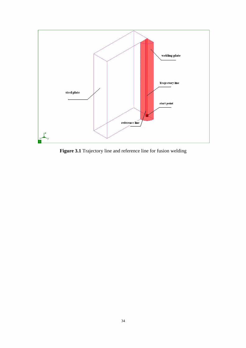
The program required that the welding heat source trajectory be explicitly
specified along the direction and position of the moving heat source using linear,
one-dimensional elements. The trajectory was chosen to be along the center line of the
whole substrate plate, with mesh size control of the weld line to ensure that the nodes
coalesced with those on the skin and volume elements. The simulation was run for
fully restrained, i.e., clamped boundary conditions.
Page 46
34
Figure 3.1 Trajectory line and reference line for fusion welding
Page 47
35
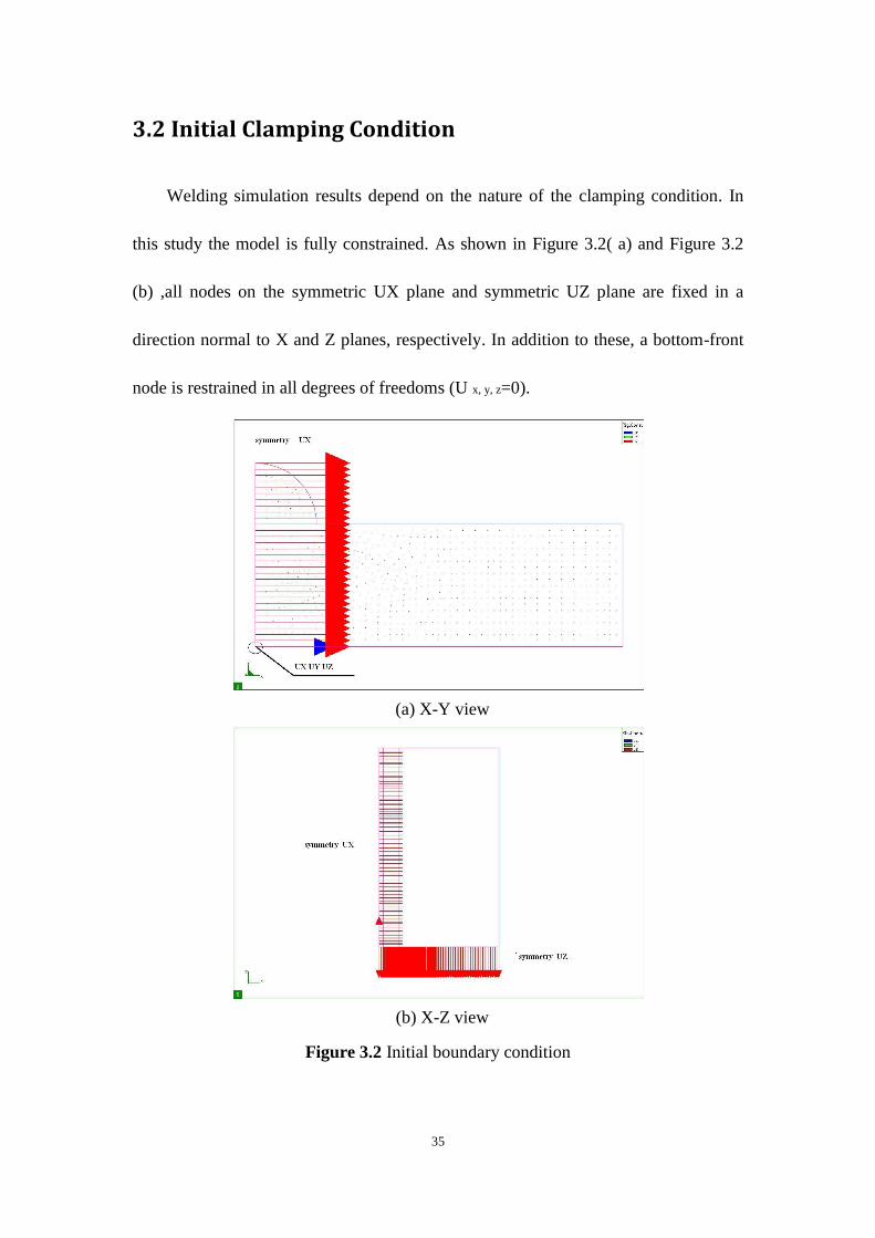
3.2 Initial Clamping Condition
Welding simulation results depend on the nature of the clamping condition. In
this study the model is fully constrained. As shown in Figure 3.2( a) and Figure 3.2
(b) ,all nodes on the symmetric UX plane and symmetric UZ plane are fixed in a
direction normal to X and Z planes, respectively. In addition to these, a bottom-front
node is restrained in all degrees of freedoms (U x, y, z=0).
(a) X-Y view
(b) X-Z view
Figure 3.2 Initial boundary condition
Page 48
36
3.3 Heat Source Modeling
The welding heat source used in this study is an arc plasma radiating intense heat
outwards with decreasing temperature. For accurate simulation of the welding heat
source, a 3-D double ellipsoidal heat source developed by Goldak [5] is usually used
in arc welding simulation. Considering a Gaussian distribution, this heat source model
has been found to be considerably more accurate than a point or a line heat source
model, especially when simulating metal gas arc welding processes [5]. The total heat
rate (q, power) from the arc welding gun is simply expressed as Eq. (3.1), with η
being the efficiency and V and I being the arc voltage and current, respectively:
[ ] (3.1)
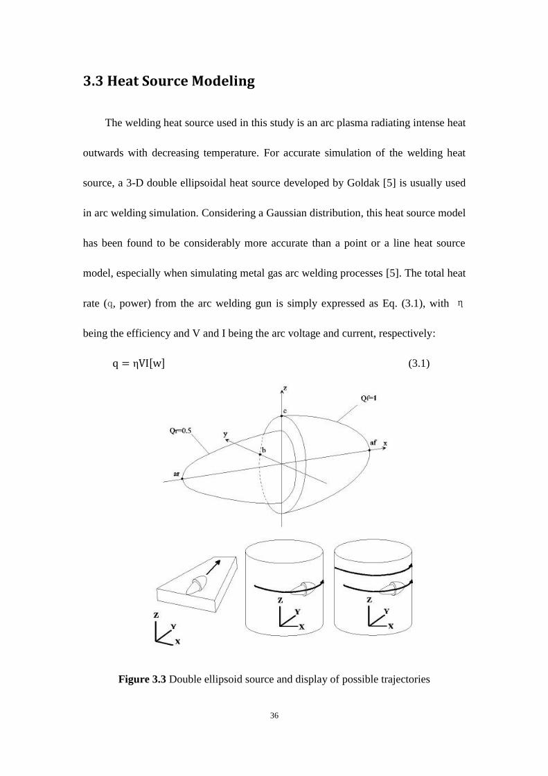
Figure 3.3 Double ellipsoid source and display of possible trajectories
Page 49
37
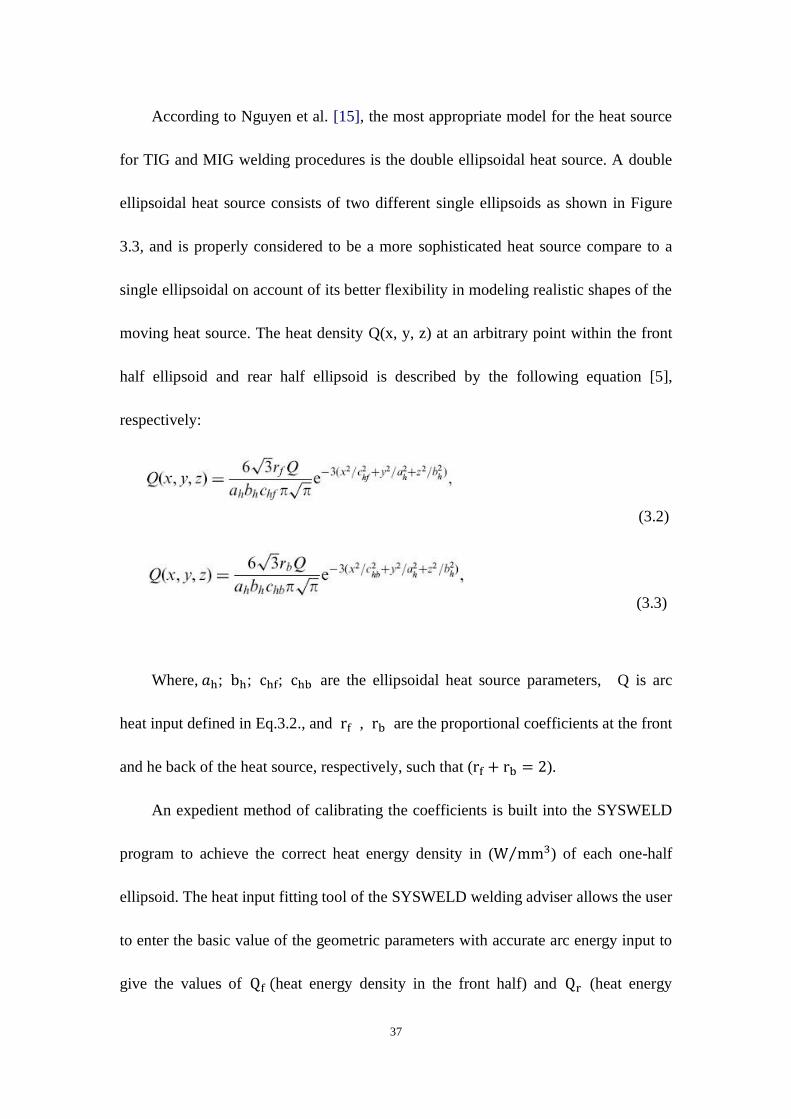
According to Nguyen et al. [15], the most appropriate model for the heat source
for TIG and MIG welding procedures is the double ellipsoidal heat source. A double
ellipsoidal heat source consists of two different single ellipsoids as shown in Figure
3.3, and is properly considered to be a more sophisticated heat source compare to a
single ellipsoidal on account of its better flexibility in modeling realistic shapes of the
moving heat source. The heat density Q(x, y, z) at an arbitrary point within the front
half ellipsoid and rear half ellipsoid is described by the following equation [5],
respectively:
(3.2)
(3.3)
Where, ; ; ; are the ellipsoidal heat source parameters, Q is arc
heat input defined in Eq.3.2., and , are the proportional coefficients at the front
and he back of the heat source, respectively, such that ( ).
An expedient method of calibrating the coefficients is built into the SYSWELD
program to achieve the correct heat energy density in ( ⁄ ) of each one-half
ellipsoid. The heat input fitting tool of the SYSWELD welding adviser allows the user
to enter the basic value of the geometric parameters with accurate arc energy input to
give the values of heat energy density in the front half) and (heat energy
Page 50
38
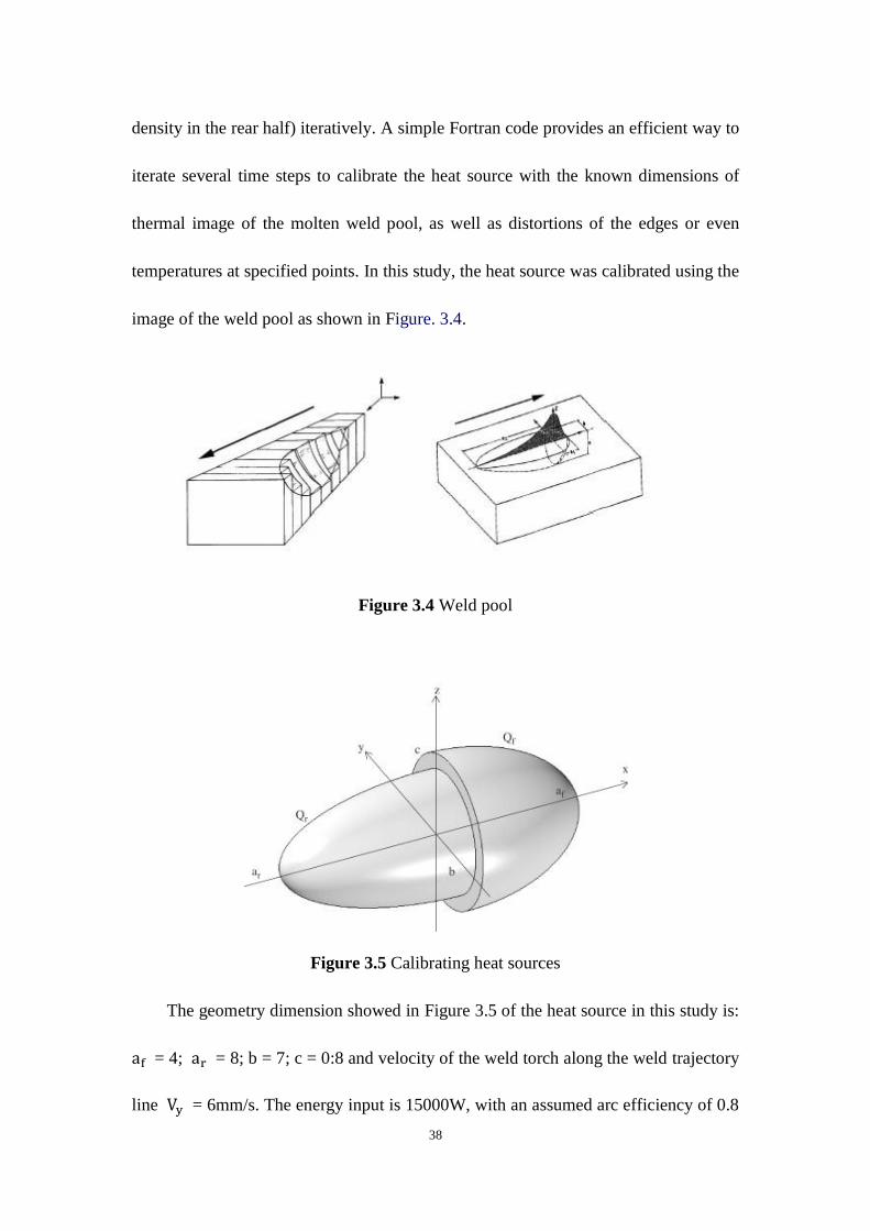
density in the rear half) iteratively. A simple Fortran code provides an efficient way to
iterate several time steps to calibrate the heat source with the known dimensions of
thermal image of the molten weld pool, as well as distortions of the edges or even
temperatures at specified points. In this study, the heat source was calibrated using the
image of the weld pool as shown in Figure. 3.4.
Figure 3.4 Weld pool
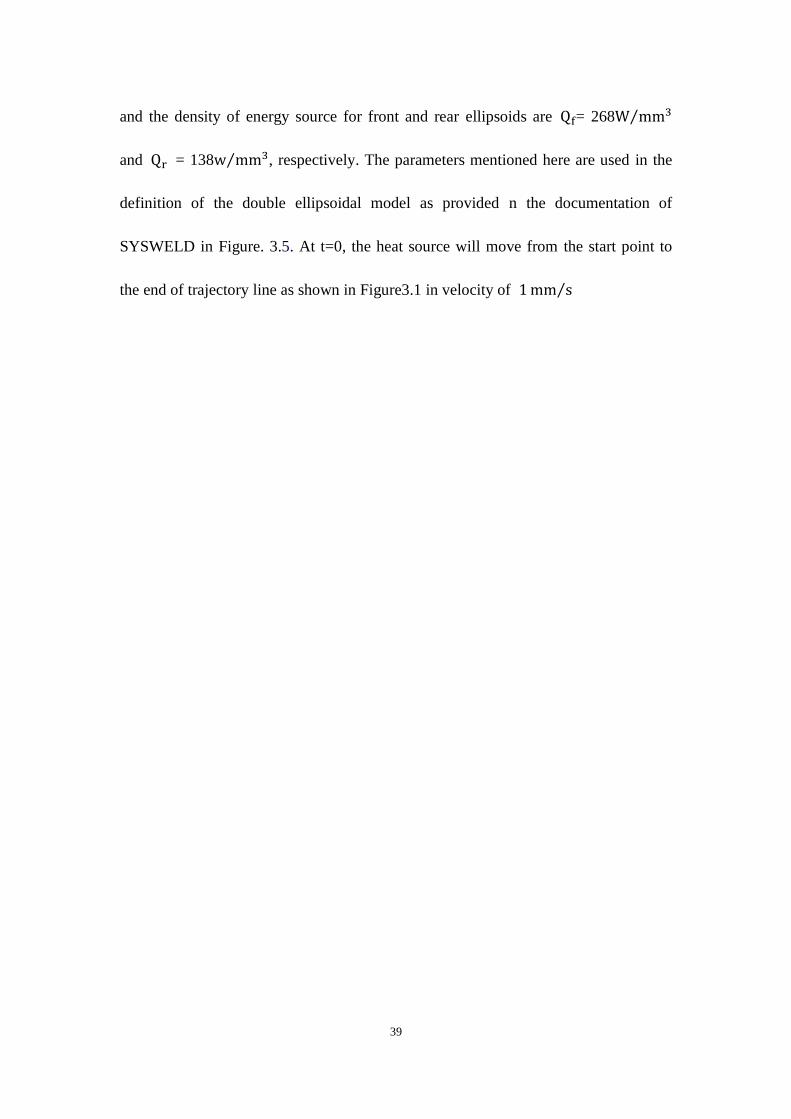
Figure 3.5 Calibrating heat sources
The geometry dimension showed in Figure 3.5 of the heat source in this study is:
= 4; = 8; b = 7; c = 0:8 and velocity of the weld torch along the weld trajectory
line = 6mm/s. The energy input is 15000W, with an assumed arc efficiency of 0.8
Page 51
39
and the density of energy source for front and rear ellipsoids are = 268 ⁄
and = 138 ⁄ , respectively. The parameters mentioned here are used in the
definition of the double ellipsoidal model as provided n the documentation of
SYSWELD in Figure. 3.5. At t=0, the heat source will move from the start point to
the end of trajectory line as shown in Figure3.1 in velocity of ⁄
Page 52
40
3.4 Heat Transfer Modeling
Radiation, convection, and conduction are considered as the main factors during
the transient heat transfer associated with welding. SYSWELD offers numerical
compute result to analysis heat transfer rates including radiation, convection and
conduction.
For radiation evaluation, the surrounding environment is specified at an ideal
temperature of 20 . In SYSWELD, the surrounding environment is created as a
group of elements as shown in Figure 2. 7 (the name of the group is skin). The “skin”
elements are used to apply the radiation boundary condition. In fundamental heat
transfer, radiation heat transfer is generally given as an expression in Equation (3.4)
where σ is the Stefan-Boltzmann constant, [ ⁄ ], and is the
emissivity, and is an ambient temperature, 20 . is defined as the radiation
heat transfer coefficient.
) ) ) )
)[
⁄ ] (3.4)
In Equation (3.4), the surface emissivity is assumed be 70% for molten stainless
steel although the emissivity is temperature-dependent. [17]. The equation is simplify
Newtonian convection:
)[
⁄ ] (3.5)
h [W/m2 K] is the convective heat transfer coefficient.
Conduction heat energy flux from the weld, which is influenced by both of the
Page 53
41
energy balance and the welding heat source and the heat transfer, is expressed in the
linear equation of the temperature gradient . In Equation (3.5), h [W/m2 K] is a
function of time (thermal conductivity) and is defined as tensor symbol
) in Cartesian coordination.
[ ⁄ ] (3.6)
The initial boundary condition for the weld surface area is expressed as Equation (3.7),
associate with radiation and convection terms [17, 18, 19]. In the Equation (3.7),
) ) (3.7)
q" is the assumed constant represent summation of the convective and radioactive heat
losses. [17]. Equation (3.7) with the heat input can be deduced as following equation
in the Cartesian coordinates, as long as heat is determined. [20, 24]
(
)
(
)
(
)
(3.8)
In equation (3.8), [ ] and [ ⁄ ]are the density and the specific
heat, respectively. Term is the thermal energy generation term and it may be
related with applied volumetric heat source or power density [ ⁄ ]. Equation
can be simplified as equation (3.9).
) (3.9)
The homogeneous equations, involving heat transfer, phase transformation and
linear plasticity, are contained in SYSWELD numerical program depended on time.
SYSWELD contains the finite element formulation of the nonlinear transient heat
transfer equations.
Page 54
42
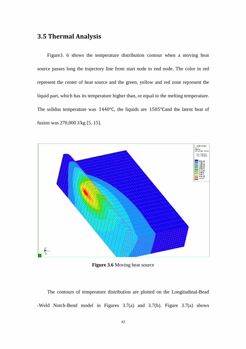
3.5 Thermal Analysis
Figure3. 6 shows the temperature distribution contour when a moving heat
source passes long the trajectory line from start node to end node. The color in red
represent the center of heat source and the green, yellow and red zone represent the
liquid part, which has its temperature higher than, or equal to the melting temperature.
The solidus temperature was , the liquids are and the latent heat of
fusion was 270,000 J/kg [5, 15].
Figure 3.6 Moving heat source
The contours of temperature distribution are plotted on the Longitudinal-Bead
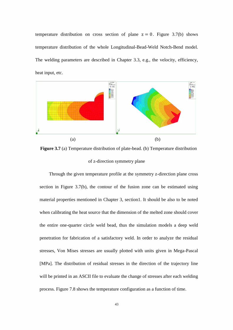
-Weld Notch-Bend model in Figures 3.7(a) and 3.7(b). Figure 3.7(a) shows
Page 55
43
temperature distribution on cross section of plane . Figure 3.7(b) shows
temperature distribution of the whole Longitudinal-Bead-Weld Notch-Bend model.
The welding parameters are described in Chapter 3.3, e.g., the velocity, efficiency,
heat input, etc.
(a) (b)
Figure 3.7 (a) Temperature distribution of plate-bead. (b) Temperature distribution
of z-direction symmetry plane
Through the given temperature profile at the symmetry z-direction plane cross
section in Figure 3.7(b), the contour of the fusion zone can be estimated using
material properties mentioned in Chapter 3, section1. It should be also to be noted
when calibrating the heat source that the dimension of the melted zone should cover
the entire one-quarter circle weld bead, thus the simulation models a deep weld
penetration for fabrication of a satisfactory weld. In order to analyze the residual
stresses, Von Mises stresses are usually plotted with units given in Mega-Pascal
[MPa]. The distribution of residual stresses in the direction of the trajectory line
will be printed in an ASCII file to evaluate the change of stresses after each welding
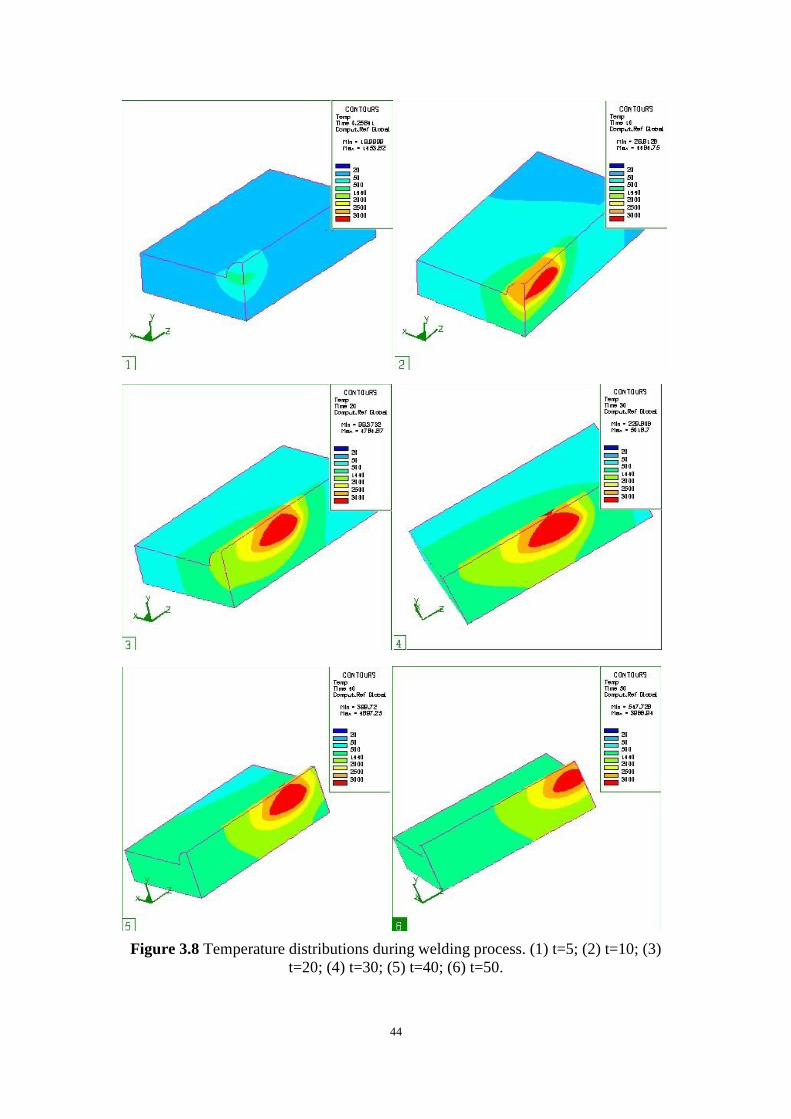
process. Figure 7.8 shows the temperature configuration as a function of time.
Page 56
44
Figure 3.8 Temperature distributions during welding process. (1) t=5; (2) t=10; (3)
t=20; (4) t=30; (5) t=40; (6) t=50.
Page 57
45
3.6 Mechanical Analysis
In SYSWELD, the mechanical analysis is based on results obtained from the
thermal analysis and is generally much more computationally intensive. The original
output data included stresses in elements, integration points and element nodes. Stress
and strain in nodes, integration points, reaction forces at nodes and other forms of
computed results can be exported by the convert and extrapolate tool that is built into
the SYSWELD ADVISOR
Page 58
46
Chapter 4.Fracture Mechanics Analysis
4.1 Finite Element code FRAC_3D
After simulation of the welding process, the computed residual stresses in the
zone of crack surface (blue zone in Figure 2.2) are exported from SYSWELD and are
imported as initial stresses into ANSYS/FRAC3D, through the
HYPERMESH/SYSWELD interface described in Chapter2, Section 4. The
methodology followed utilizes the same FE mesh for both numerical analyses in order
to simplify the transfer of data between the two simulations.
The finite element program FRAC3D is specifically designed to treat crack
problems in fracture mechanics with a stress singularity at the tip of the crack. The
enriched crack tip element formulation for 2-D problem begins from Benzley's work
[20], and is generalized such that any singularity may be represented by including the
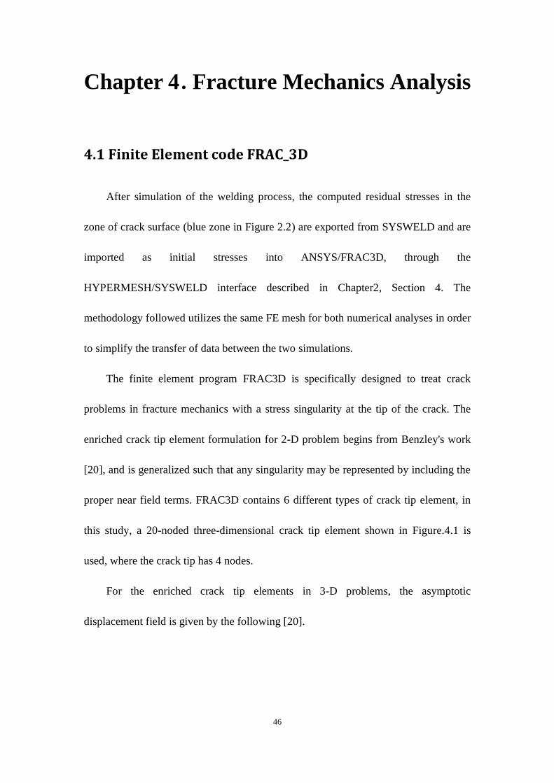
proper near field terms. FRAC3D contains 6 different types of crack tip element, in
this study, a 20-noded three-dimensional crack tip element shown in Figure.4.1 is
used, where the crack tip has 4 nodes.
For the enriched crack tip elements in 3-D problems, the asymptotic
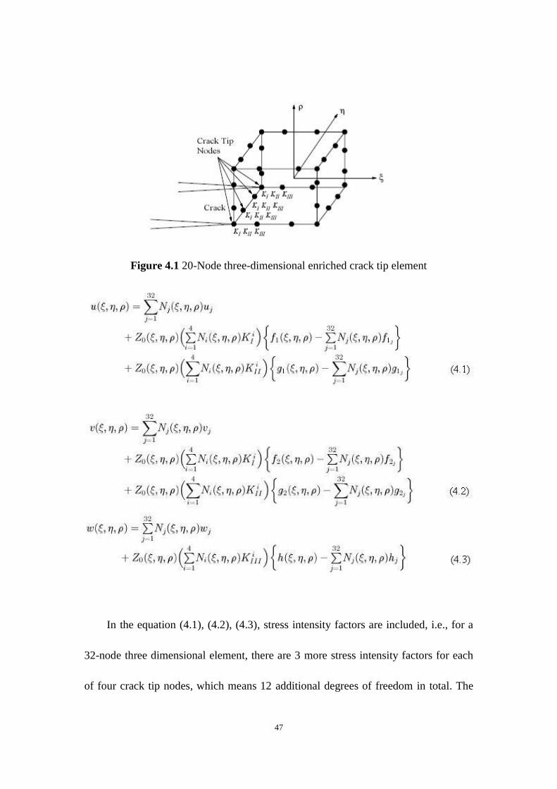
displacement field is given by the following [20].
Page 59
47
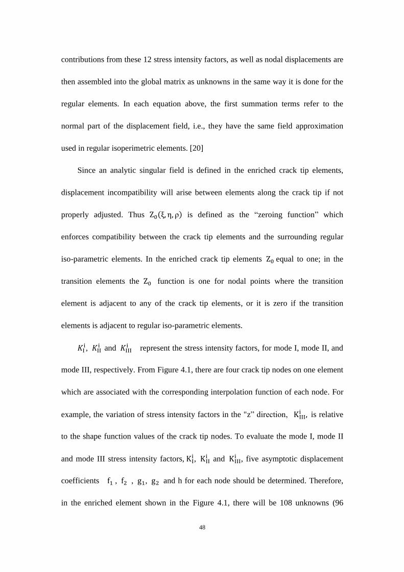
Figure 4.1 20-Node three-dimensional enriched crack tip element
In the equation (4.1), (4.2), (4.3), stress intensity factors are included, i.e., for a
32-node three dimensional element, there are 3 more stress intensity factors for each
of four crack tip nodes, which means 12 additional degrees of freedom in total. The
Page 60
48
contributions from these 12 stress intensity factors, as well as nodal displacements are
then assembled into the global matrix as unknowns in the same way it is done for the
regular elements. In each equation above, the first summation terms refer to the
normal part of the displacement field, i.e., they have the same field approximation
used in regular isoperimetric elements. [20]
Since an analytic singular field is defined in the enriched crack tip elements,
displacement incompatibility will arise between elements along the crack tip if not
properly adjusted. Thus ) is defined as the “zeroing function” which
enforces compatibility between the crack tip elements and the surrounding regular
iso-parametric elements. In the enriched crack tip elements equal to one; in the
transition elements the function is one for nodal points where the transition
element is adjacent to any of the crack tip elements, or it is zero if the transition
elements is adjacent to regular iso-parametric elements.
,
and
represent the stress intensity factors, for mode I, mode II, and
mode III, respectively. From Figure 4.1, there are four crack tip nodes on one element
which are associated with the corresponding interpolation function of each node. For
example, the variation of stress intensity factors in the "z” direction, is relative
to the shape function values of the crack tip nodes. To evaluate the mode I, mode II
and mode III stress intensity factors, ,
and
, five asymptotic displacement
coefficients , , , and h for each node should be determined. Therefore,
in the enriched element shown in the Figure 4.1, there will be 108 unknowns (96
Page 61
49
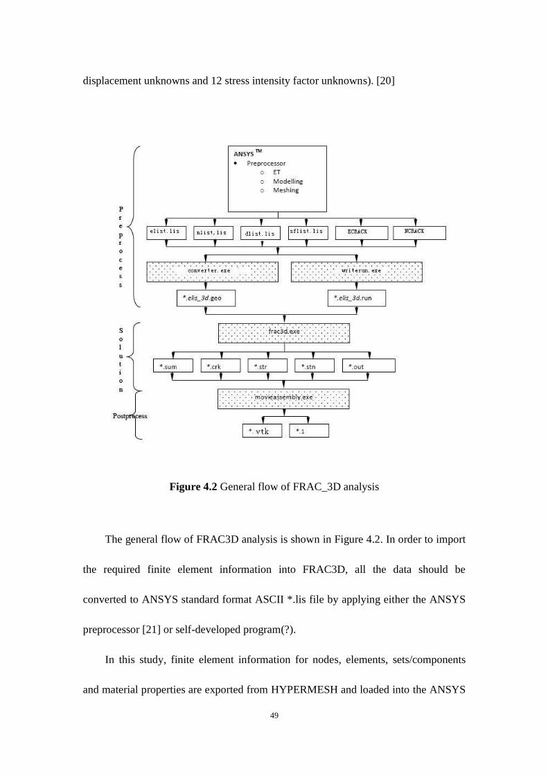
displacement unknowns and 12 stress intensity factor unknowns). [20]
Figure 4.2 General flow of FRAC_3D analysis
The general flow of FRAC3D analysis is shown in Figure 4.2. In order to import
the required finite element information into FRAC3D, all the data should be
converted to ANSYS standard format ASCII *.lis file by applying either the ANSYS
preprocessor [21] or self-developed program(?).
In this study, finite element information for nodes, elements, sets/components
and material properties are exported from HYPERMESH and loaded into the ANSYS
Page 62
50
preprocessor directly by utilizing the built in HYPERMESH interface with ANSYS
program. As shown in Figure 4.2, six files are required to prepare for analysis in
FRAC_3D. In this thesis, five files are exported from ANSYS and one is created
using a FORTRAN program that will be described in Chapter 4 Section2 from stress
data generated by SYSWELD. For the five files, elist.lis file provides the finite
element connectivity information; nlist.lis contains nodal coordinate data; dlist.lis
contains boundary conditions; and ECRACK and NCRACK represent crack element
file and crack tip element file (what‟s the difference between these two files?),
respectively. The file sflist.lis is a pressure file generated by a FORTRAN program
and contains the pressure on the crack surface from fusion welding simulation. In the
process of creating a *.elsit_3d.goe file, it was necessary to constrain
and to
zero along the whole crack front, since the problem should be symmetric by definition.
Another assumption is that there shouldn‟t be any shear stresses on the cross-section,
since in this study only mode I loading is permitted.
Page 63
51
4.2 SYSWELD/FRAC3D Interface
The SYSWELD/FRAC3D Interface generates a file contains pressures on the
crack surface. This file is used in the superposition methodology which is the most
expedient approach to solve problem of Longitudinal-Bead-Weld plate with a notch.
The purpose of this step is to use the SYSWELD stresses that are transferred only for
the zone where the crack surface will be in the ANSYS/FRAC3D model. Then these
stresses will be applied to the crack surface as pressure. There should be no other
loads acting on the FRAC3D model with all other boundary conditions the same. In
this approach the initial stresses normal to the weld cross-section are applied as a
pressure on the crack surface. When applying pressure to a surface, the finite element
program will compute the correct consistent nodal forces that are work equivalent to
the pressure distribution. It should be noted that this Interface does not determine
these forces directly; i.e., the FEM software determines theses nodal forces. This
approach will give the correct stress intensity factors in FRAC3D.
Typically most finite element programs provide two sets of stress output. The
element by element output gives the stress components at the nodes, which is
extrapolated from the integration points within that particular element. These stresses
are fairly accurate, but the nodal stresses are not the same for nodes shared by the
different elements, i.e., the stresses between elements are averaged at the nodes. The
second stress information that's usually output is the averaged nodal stresses. This
results in a stress smoothing that gives a reasonably good representation of the state of
Page 64
52
stress at the nodes. The only time that average nodal stresses are not accurate, is when
the node is shared by two adjacent elements that have different material properties. In
this special case, there is a stress discontinuity in the component of stress parallel to
the element boundary. Of course, this is not an issue in the problems that this study is
dealing with. Thus, for the superposition calculations in this study, the averaged
stresses that are given for the nodes, instead of the nodal stresses that are given by the
individual elements are used for fusion welding residual stress transfer.
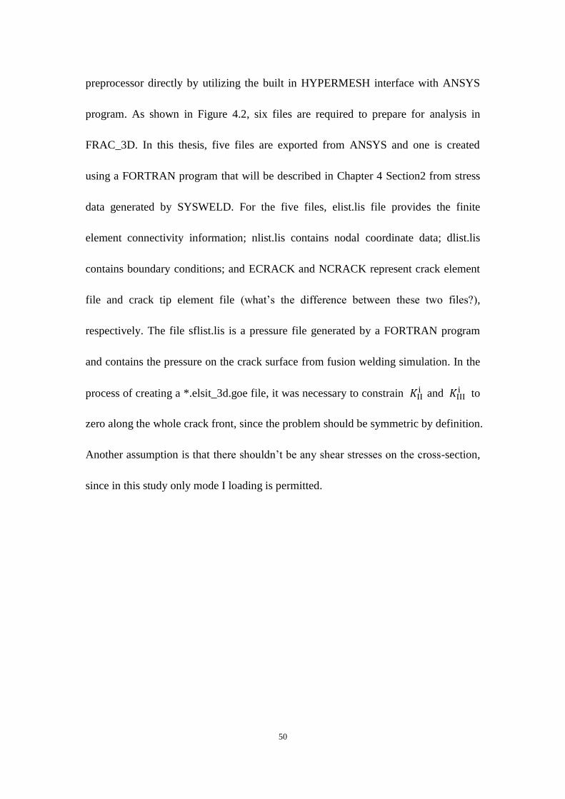
Figure 4.3 Surface Loads Pressures format, face 1: (J-I-L-K), face 2: (I-J-N-M), face 3
(J-K-O-N), face 4: K-L-P-O), face 5: (L-I-M-P), face 6 (M-N-O-P)
When applying residual stress as pressure, ANSYS file require four nodal
stresses for each quadratic HEAX20/3020/SOLID95 element on the crack surface.
The point and the number are shown in Figure 4.3. For example, in
Page 65
53
SYSWELD/FRAC3D Interface, the program automatically picks four corner nodes J,
I, L, K in face 1 which is shown in Figure 4.3.
Page 66
54
4.3 Superposition Results
The purpose of this section is to describe the process of superimposing the
stresses from the un-cracked configuration obtained from SYSWELD to the cracked
configuration in FRAC3D to obtain the correct stress intensity factors. The
superposition process can be used to obtain the stress result for the whole
configuration, if the stresses obtained from both configurations are added together.
However, since the most important result from a fracture mechanics point of view is
the stress intensity factor values obtained from FRAC3D, it is usually unnecessary to
generate the entire stress state. In this study, the main purpose of merging the two
stress states is to provide an overall sense of the state of stress in the cracked
configuration.
From the flow chart shown in Figure 4.2, the FRAC3D output information is
saved in six ASCII files. Among the six files, the *.crk file gives the computed stress
intensity factor along the crack front tip..
When applying pressure to the crack surface, the crack surface will not be stress
free, though this will give the correct stress intensity factors. To obtain the actual
stresses in the cracked structure, it is necessary to add the FRAC3D nodal stresses to
the initial stresses from SYSWELD. For example, if the initial stresses from
SYSWELD on the plane where the crack surface is located are tensile stresses, when
these stresses are applied as pressure on the crack surface in FRAC3D, the result will
be compressive stresses at the nodes on the crack surface. Thus, if the positive initial
Page 67
55
stresses from SYSWELD are added to the compressive stresses on the crack surface
from FRAC3D, they cancel out and will yield a stress-free crack surface. The stresses
everywhere else in the model can be obtained by superposing the stresses from the
two calculations.
The *.str file provides stress tensor information for each element in Cartesian
coordinates. In the stress output for each element, there is the effective stress , the
normal stress component in the x direction , stress in y direction , stress in z
direction , and shear stress component xy , shear stress yz , shear stress xz
for each node in the element. When superposing components of the stress tensor
in a specific direction, the FORTRAN program first adds the two sets of
from fusion welding simulation and fracture mechanics
analysis together; then new effective stresses are recalculated use equation. This will
provide a stress free crack surface.
√ √ ) ) ) ) ) )
(4.4)
) (4.5)
The *.stn file provides strain tensor information for each element in Cartesian
coordinate. In the strain tensor for each element, there is the effective strain ,
strain in xx direction strain in yy direction , strain in zz direction , strain in
Page 68
56
xy direction , strain in yz direction , strain in xz direction for each node in the
element When superposed strain tensors, the FORTRAN program first recalculated
uses the same procedure for computing stresses. New effective
strains are equal to zero, because this is not a general plane stress problem. The result
will provide the total strain configuration.
The *.out file from FRAC3D contains three sections of data output in Cartesian
coordinates. Firstly, it provides displacement in x, y, z direction for each node, which
provides a total displacement configuration. Secondly, it lists average stress tensor in
xx, yy, zz, xy, yz, xz direction for each node. Last is the nodal reaction forces in x, y,
z direction for each node. And they will be added together directly.
After all results in these three files are superposed, they are written by a
FORTRAN program to a Python standard format file. As shown in Figure 4.2,
ultimately two files,*.1 file and *.vtk file, are created to generate visible stress, strain,
and displacement contour plots in the PARAVIEW program.
Page 69
57
Chapter 5.Conclusions and Furture
Work
5.1 Finite element analysis of crack problems
In this chapter, the results of fusion welding simulation and fracture mechanics
analysis are summarized in terms of residual stress and stress intensity factor at the
crack front.
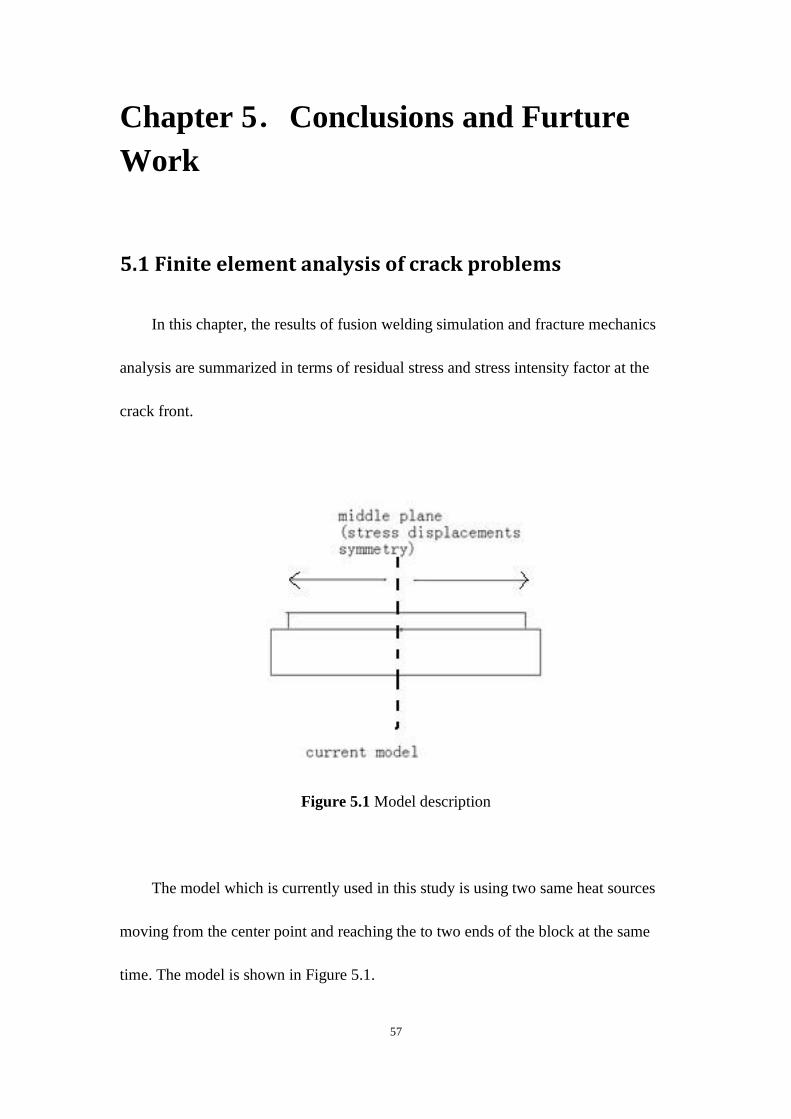
Figure 5.1 Model description
The model which is currently used in this study is using two same heat sources
moving from the center point and reaching the to two ends of the block at the same
time. The model is shown in Figure 5.1.
Page 70
58
Currently the middle plane should be the symmetry plane because the movement
of heat sources and heat transfer process should be symmetry on middle plane. Thus,
stresses, strains displacements and other results of the right part and the left part will
be symmetry.
The result generally includes: 1) temperature distribution as a function of time, 2)
temperature shortly after welding process; 3) temperature distribution after cooling; 4)
Von Mises stress configuration as a function of time; 4) residual stress as a function
of time; 5) stress intensity factor along the crack front; 5) total stress configuration; 6)
displacement configuration.
1. General mesh for large front case
Figure 5.1 shows the temperature distribution in five cross-section views
perpendicular to the welding direction. The geometry is described in chapter 2.2. In
this model the crack front is represented by a part of a arc whose radius is 12
mm. The welding parameters are described in Chapter 3.1, 3.2 and 3.3. Temperatures
on elements along the crack front after cooling are compared in Figure 5.3. Residual
stress distributions can be found in Figure 5.4, where five cross-section views are
selected along the fusion welding direction to represent the global configuration
results from the fusion welding process after the part has cooled down. It should be
noted that the part is still full clamped in these images. Figure 5.5(1) shows the total
configuration after superposition of welding stress output and FRAC3D analysis.
Page 71
59
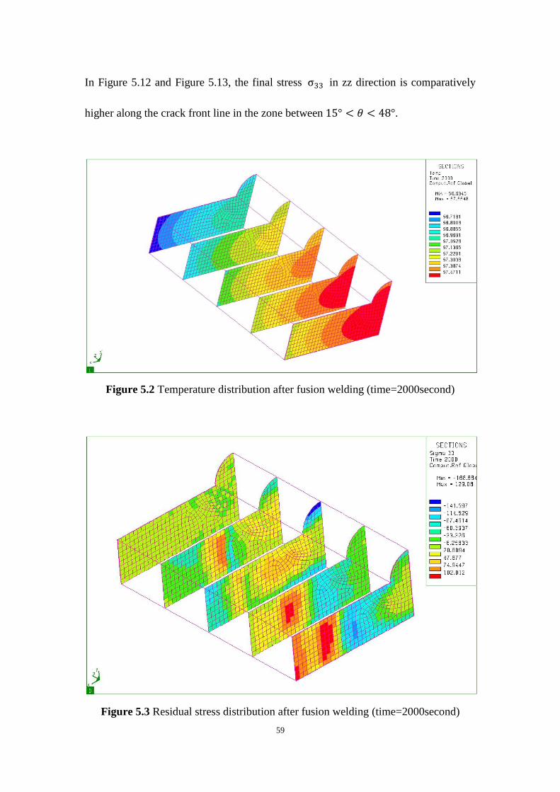
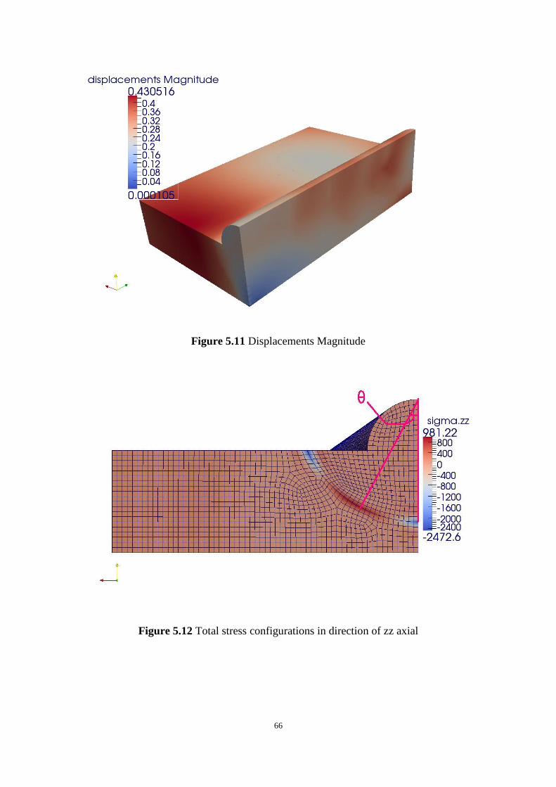
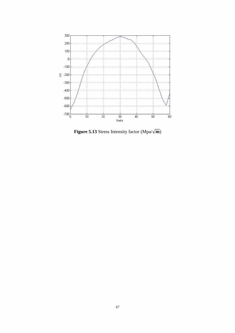
In Figure 5.12 and Figure 5.13, the final stress in zz direction is comparatively
higher along the crack front line in the zone between .
Figure 5.2 Temperature distribution after fusion welding (time=2000second)
Figure 5.3 Residual stress distribution after fusion welding (time=2000second)
Page 72
60
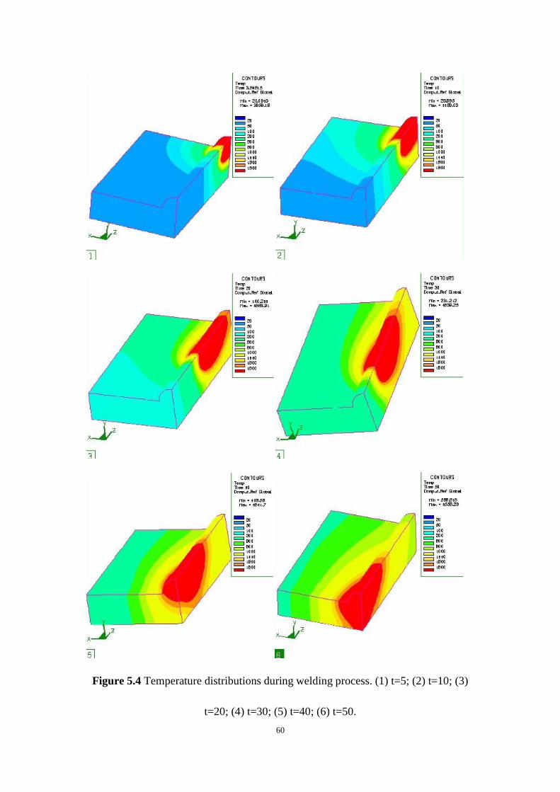
Figure 5.4 Temperature distributions during welding process. (1) t=5; (2) t=10; (3)
t=20; (4) t=30; (5) t=40; (6) t=50.
Page 73
61
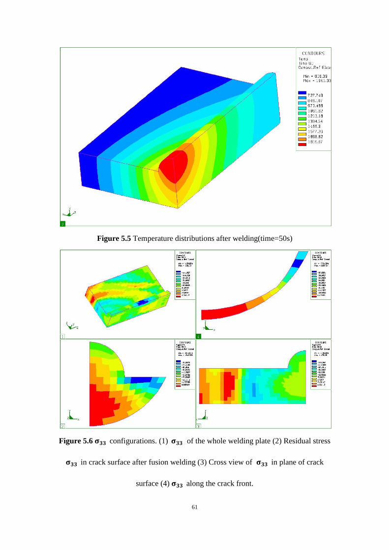
Figure 5.5 Temperature distributions after welding(time=50s)
Figure 5.6 configurations. (1) of the whole welding plate (2) Residual stress
in crack surface after fusion welding (3) Cross view of in plane of crack
surface (4) along the crack front.
Page 74
62
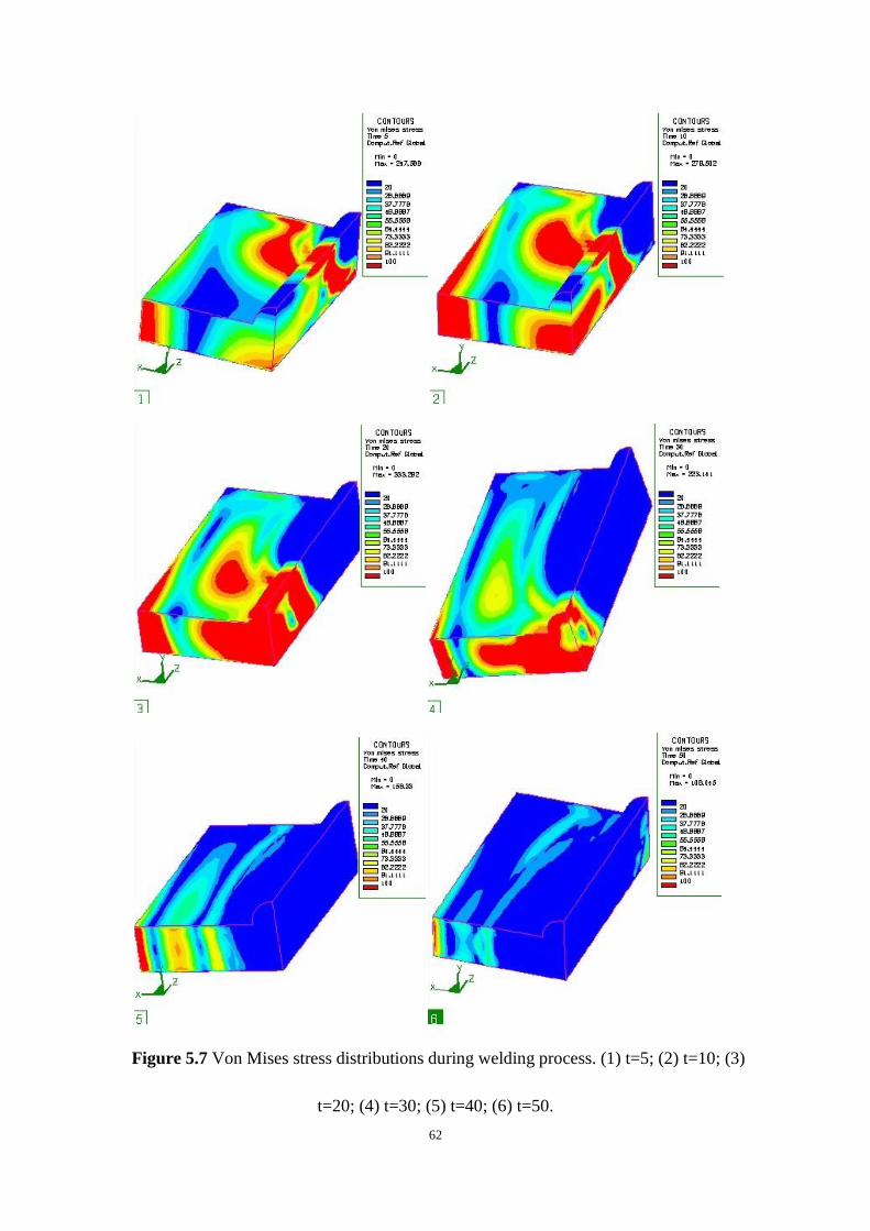
Figure 5.7 Von Mises stress distributions during welding process. (1) t=5; (2) t=10; (3)
t=20; (4) t=30; (5) t=40; (6) t=50.
Page 75
63
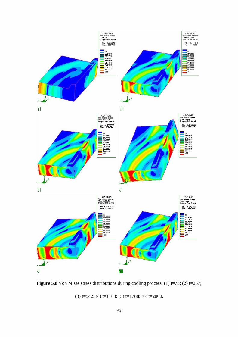
Figure 5.8 Von Mises stress distributions during cooling process. (1) t=75; (2) t=257;
(3) t=542; (4) t=1183; (5) t=1788; (6) t=2000.
Page 76
64
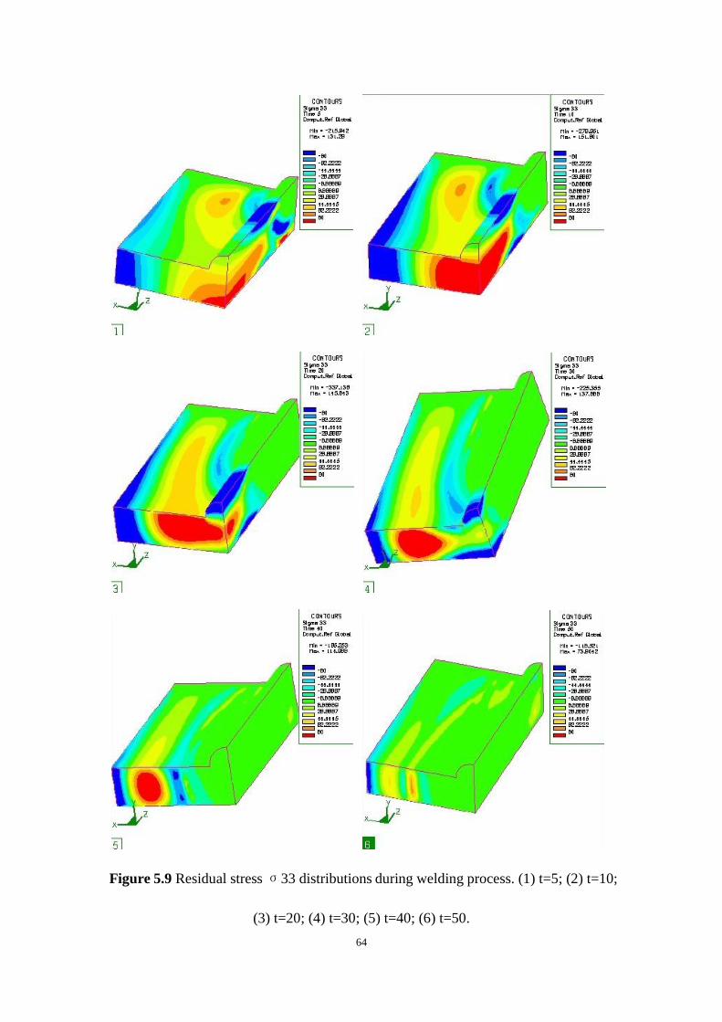
Figure 5.9 Residual stress σ33 distributions during welding process. (1) t=5; (2) t=10;
(3) t=20; (4) t=30; (5) t=40; (6) t=50.
Page 77
65
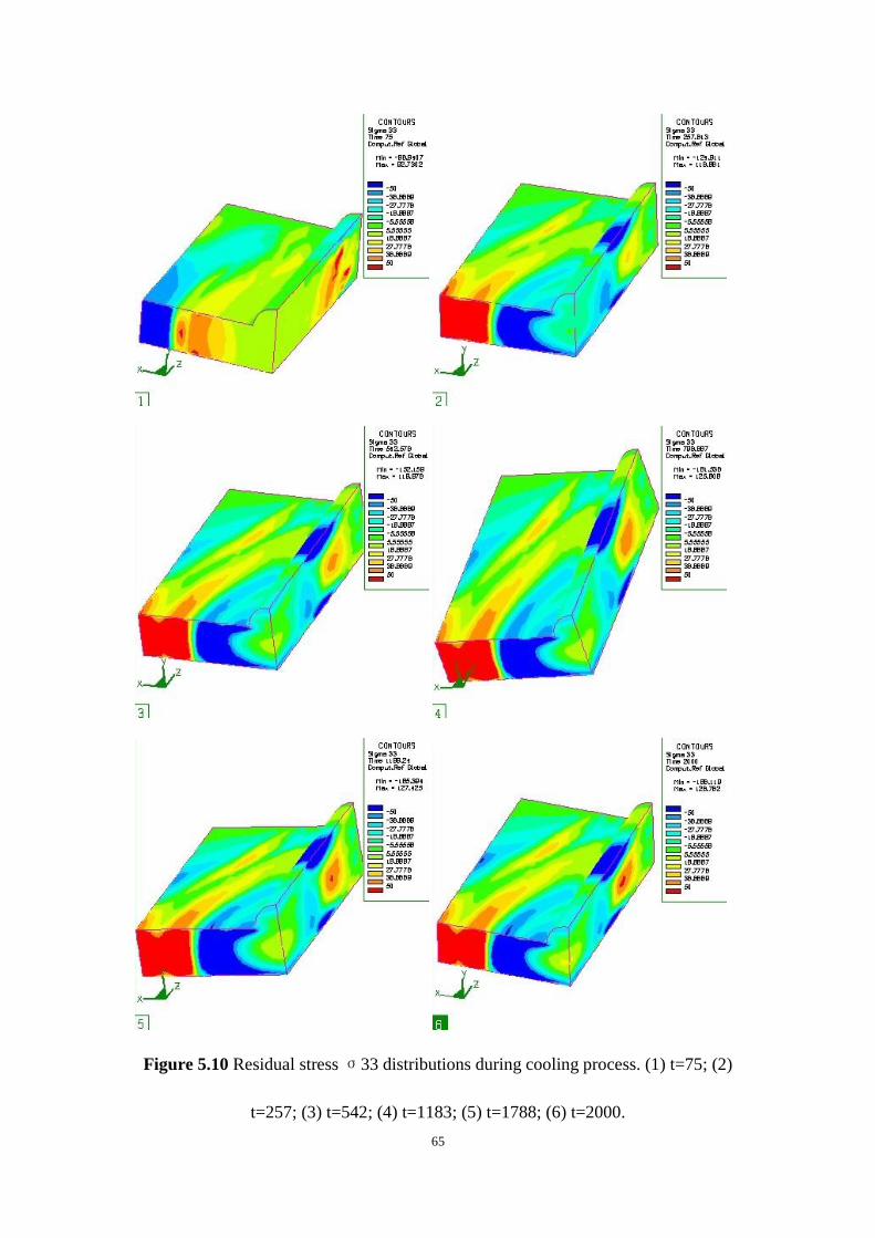
Figure 5.10 Residual stress σ33 distributions during cooling process. (1) t=75; (2)
t=257; (3) t=542; (4) t=1183; (5) t=1788; (6) t=2000.
Page 78
66
Figure 5.11 Displacements Magnitude
Figure 5.12 Total stress configurations in direction of zz axial
Page 79
67
Figure 5.13 Stress Intensity factor (Mpa/√ )
Page 80
68
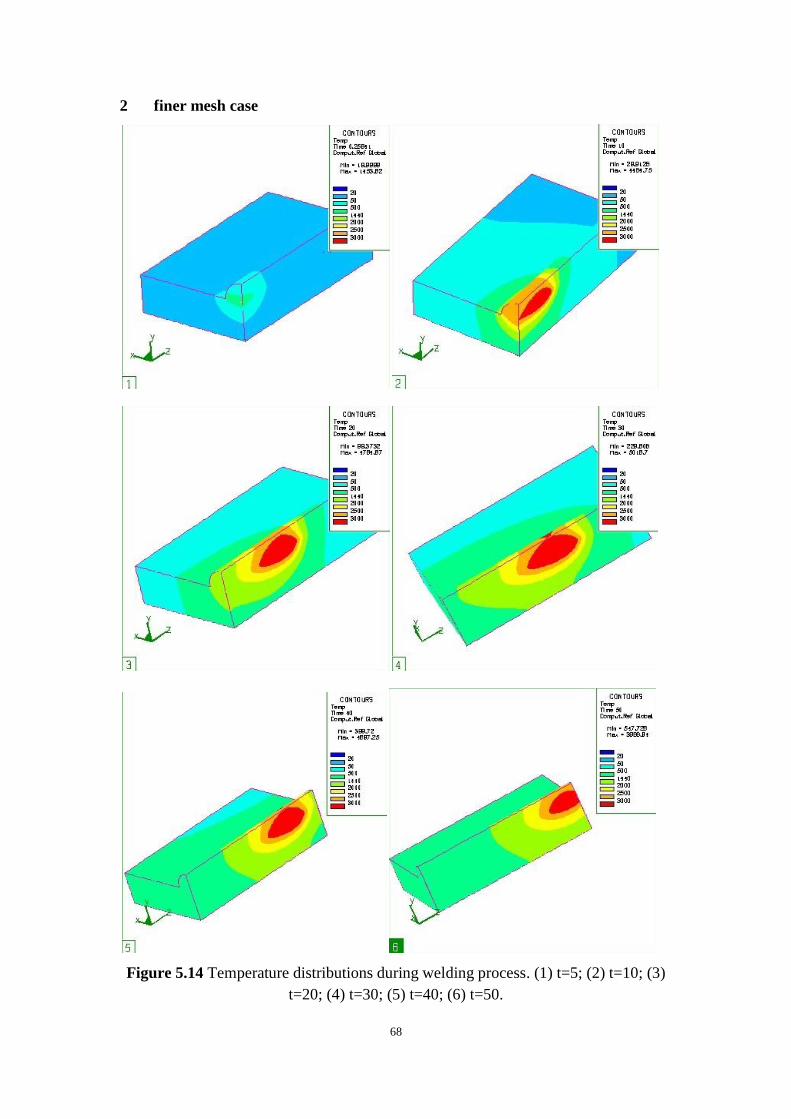
2 finer mesh case
Figure 5.14 Temperature distributions during welding process. (1) t=5; (2) t=10; (3)
t=20; (4) t=30; (5) t=40; (6) t=50.
Page 81
69
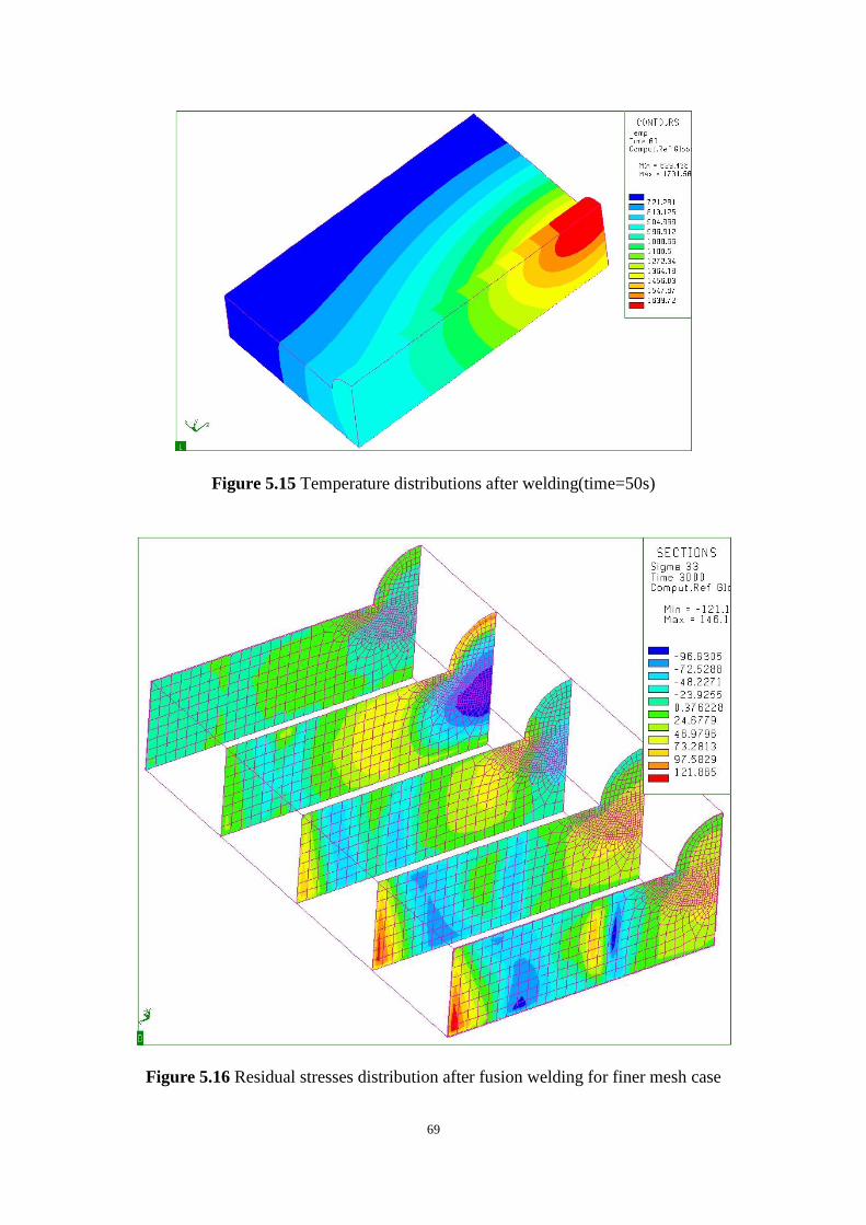
Figure 5.15 Temperature distributions after welding(time=50s)
Figure 5.16 Residual stresses distribution after fusion welding for finer mesh case
Page 82
70
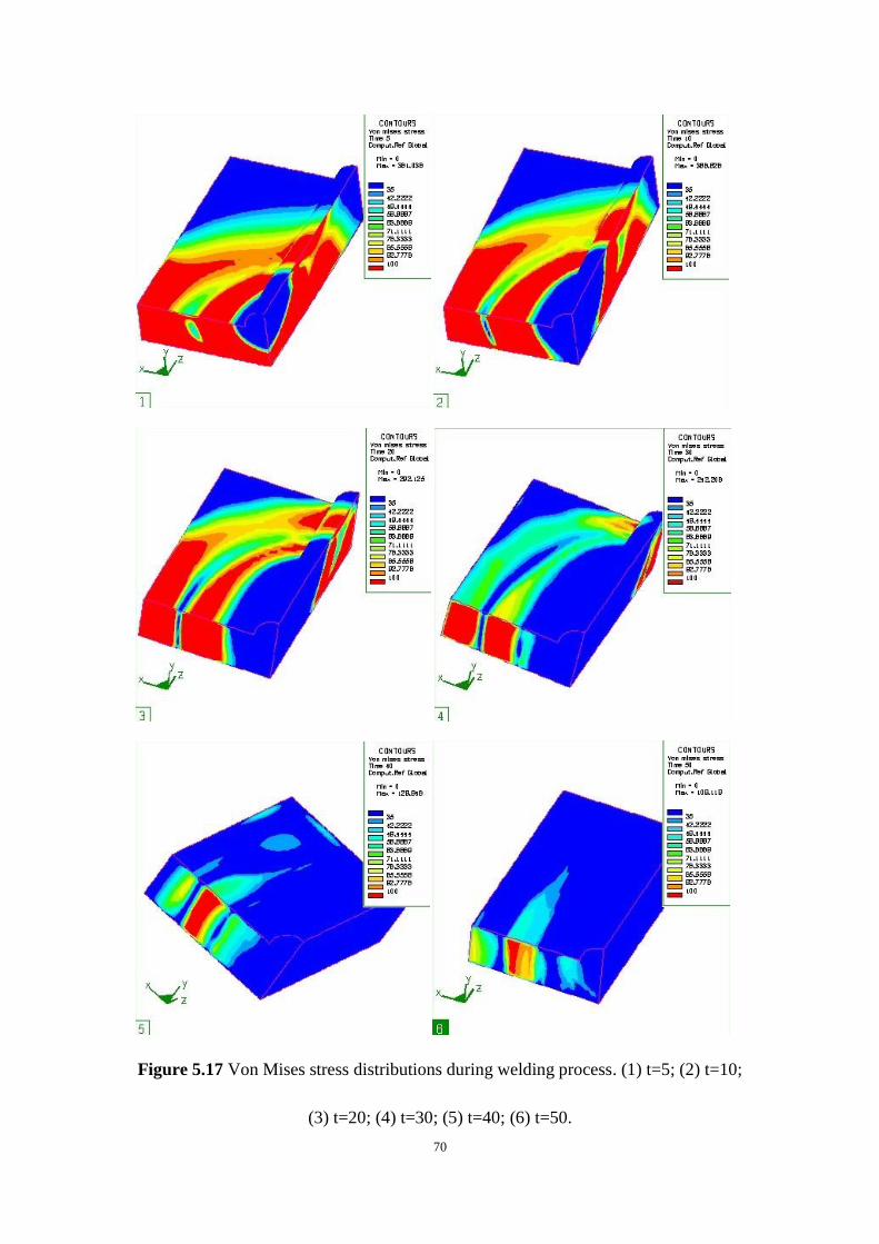
Figure 5.17 Von Mises stress distributions during welding process. (1) t=5; (2) t=10;
(3) t=20; (4) t=30; (5) t=40; (6) t=50.
Page 83
71
Figure 5.18 Von Mises stress distributions during cooling process. (1) t=75; (2) t=257;
(3) t=542; (4) t=1183; (5) t=1788; (6) t=3000.
Page 84
72
Figure 5.19 Residual stress σ33 distributions during welding process. (1) t=5; (2)
t=10; (3) t=20; (4) t=30; (5) t=40; (6) t=50.
Page 85
73
Figure 5.20 Residual stress σ33 distributions during cooling process. (1) t=75; (2)
t=257; (3) t=542; (4) t=1183; (5) t=1788; (6) t=3000.
Page 86
74
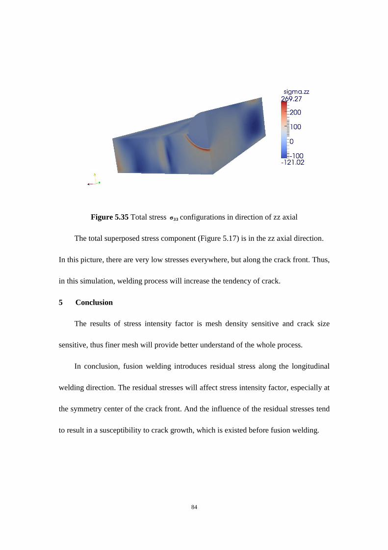
Figure 5.21 configuration for finer mesh case. (1) of the whole welding plate.
(2) Residual stress in crack surface after fusion welding (3) Cross view of in
plane of crack surface. (4) along the crack front.
Figure 5.22 Stress intensity factor k1 (Mpa/√ )
Page 87
75
3 coarser mesh case
Figure 5.23 Residual stresses distribution after fusion welding for coarser mesh case
Figure 5.24 σ33 configuration for coarser mesh case. (1) σ33 of the whole welding
plate. (2) Residual stressσ33 in crack surface after fusion welding. (3) Cross view
ofσ33 in plane of crack surface. (4) σ33 along the crack front.
Page 88
76
Figure 5.25 Stress intensity factor k1 (Mpa/√ ).
Section two and section one use the same geometry which is described in
Chapter2, section2. Compare figure 5.24 and 5.23, the residual stress exported form
fusion welding simulation is sensitive to mesh density. Figure 5.22 uses finer mesh
along the crack front and the heat source path, thus the residual stress is positive
which means the crack will be extravagant. The reason why Figure 5.25 is negative is
probably that the element density and welding run time is not high enough. Negative
SIF is a compressive state of stress that is a result of prevent the material from
expanding.
Page 89
77
4 refined small front mesh case
Figure 5. 26 Temperature distributions during welding process. (1) t=5; (2) t=10; (3)
t=20; (4) t=30; (5) t=40; (6) t=50.
Page 90
78
Figure 5.27 Temperature distributions after welding(time=50s)
Figure 5.28 Residual stresses distribution after cooling for smaller front (t=3000s)
Page 91
79
Figure 5.29 Von Mises stress distributions during welding process. (1) t=5; (2) t=10;
(3) t=20; (4) t=30; (5) t=40; (6) t=50.
Page 92
80
Figure 5.30 Von Mises stress distributions during cooling process. (1) t=75; (2) t=257;
(3) t=542; (4) t=1183; (5) t=1788; (6) t=3000.
Page 93
81
Figure 5.31 Residual stress σ33 distributions during welding process. (1) t=5; (2)
t=10; (3) t=20; (4) t=30; (5) t=40; (6) t=50.
Page 94
82
Figure 5.32 Residual stress σ33 distributions during cooling process. (1) t=75; (2)
t=257; (3) t=542; (4) t=1183; (5) t=1788; (6) t=3000.
Page 95
83
Figure 5.33 σ33 configuration after cooling for smaller front case. (1) σ33 of the whole
welding plate after cooling. (2) Residual stressσ33 in crack surface after cooling. (3) Cross view
ofσ33 in plane of crack surface after cooling. (4) σ33 along the crack front after cooling.
Figure 5.34 Stress intensity factor k1 (Mpa/√ ).
Page 96
84
Figure 5.35 Total stress configurations in direction of zz axial
The total superposed stress component (Figure 5.17) is in the zz axial direction.
In this picture, there are very low stresses everywhere, but along the crack front. Thus,
in this simulation, welding process will increase the tendency of crack.
5 Conclusion
The results of stress intensity factor is mesh density sensitive and crack size
sensitive, thus finer mesh will provide better understand of the whole process.
In conclusion, fusion welding introduces residual stress along the longitudinal
welding direction. The residual stresses will affect stress intensity factor, especially at
the symmetry center of the crack front. And the influence of the residual stresses tend
to result in a susceptibility to crack growth, which is existed before fusion welding.
Page 97
85
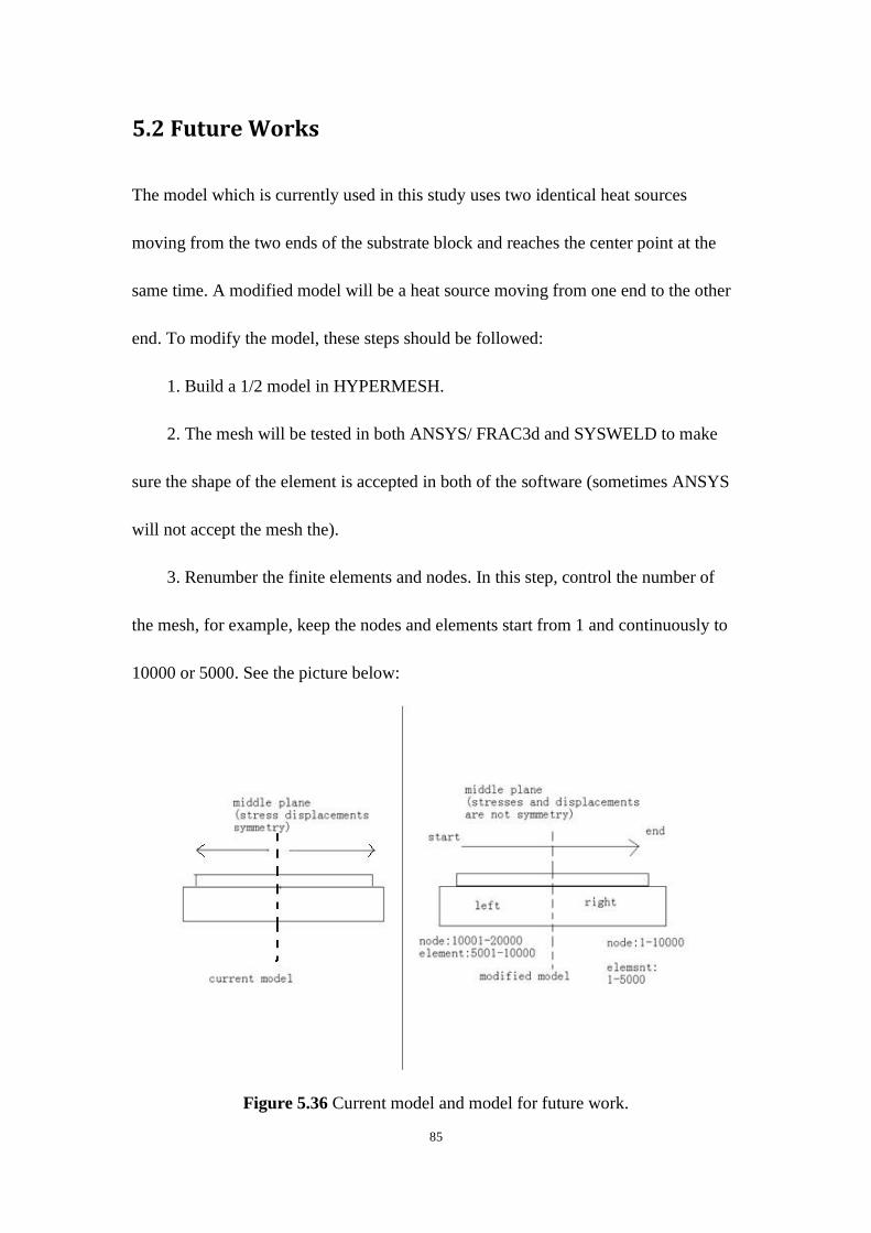
5.2 Future Works
The model which is currently used in this study uses two identical heat sources
moving from the two ends of the substrate block and reaches the center point at the
same time. A modified model will be a heat source moving from one end to the other
end. To modify the model, these steps should be followed:
1. Build a 1/2 model in HYPERMESH.
2. The mesh will be tested in both ANSYS/ FRAC3d and SYSWELD to make
sure the shape of the element is accepted in both of the software (sometimes ANSYS
will not accept the mesh the).
3. Renumber the finite elements and nodes. In this step, control the number of
the mesh, for example, keep the nodes and elements start from 1 and continuously to
10000 or 5000. See the picture below:
Figure 5.36 Current model and model for future work.
Page 98
86
In the same time elements and nodes in left part will continuously start from
5001, and from 10001, respectively.
4. Create room temperature model and weld line model. Renumber them
5. Create groups which are needed in SYSWELD simulation.
6. Save the model in another file. Delete the whole left part. Create groups which
will be used to generate files for FRAC3D.( I am not quite sure if this step can be
done)
7. Perform welding simulation for 1/2 model.(this need 48 hours if I run it on our
work station)
8. Export residual stress.
9. Perform FRAC3D computation.
10. Superposition SYSWELD result and Frac3D result.
In future work, the method of this study can be used to study the effect that
different welding parameters have on the fracture parameters.
Page 99
87
References
[1] A. O. Ayhan, H. F. Nied,Frac3D-Finite Element Based Software for 3-D and
Generalized Plane Strain Fracture Analysis(second version), Mechanical
Engineering and Mechanics, Lehigh University.
[2] A. O. Ayhan, H. F. Nied, “Stress intensity factors for three-dimensional surface
cracks using enriched finite elements”, International Journal for Numerical Methods
in Engineering, 54:899-921, 2002.
[3] A. O. Ayhan, A. C. Kaya, H. F. Nied, “Analysis of three-dimensional interface
cracks using enriched finite elements”, International Journal of Fracture,
142,:255-276, 2006.
[4]ANSYS®, User‟s manual, 2010.
[5]SYSWELD®, User‟s manual, ESI Group, 2010.
[6] Suraj Joshi, Cumali Semetay, John WH Price and Herman F. Nied. Weld-induced
residual stresses in a prototype dragline cluster and comparison with design codes.
Thin-Walled Structures. Volume 48, Issue 2, February 2010, Pages 89-102
[7] Cumali Senetay, Hussam Mahmoud, Herman F. Nied. Stress and fracture analysis
for welded plate Girders in Bridge structures. In: Department of Mechanical
Engineering and Mechanics, Lehigh University.
[8]HYPERMESH®, User‟s manual, 2010.
[9] Herman F. Nied. and S. Marugan, Murat Ozturk, Ergun Nart, Aaron Mengel,
Page 100
88
Erman Citirik. Finite element modeling of residual stress and distortion from
welding stainless steel structures. ATLSS report ; no. 04-06.
[10]Michaleris P, Kirk M, Mohr W, McGaughy T. Incorporation of residual stress
effects into fracture assessment via the finite element method. Fatigue and fracture
mechanics. In: Underwood JH, Macdonald BD, Mitchell MR, editors. American
society for testing and materials, vol. 28. ASTM STP 1321; 1997.
[11] V. Robin, T. Pyttfl, J. Christlein, A. Strating. fracture analysis of welded
components. In: ESI France, Lyon, France. ESI Gmbh, Eschborn , Germany. AUDI
AG, Neckarsulm, Germany,
[12]Z.Barsoum. Residual stress analysis and fatigue of multi-pass welded tubular
structures. Royal Institute of Technology, department of Aeronautical and Vehicle
Engineering, Teknikringen 8, 100 44 Stockholm, Sweden. Engineering Failure
Analysis 15 (2008) 863–874
[13] E.Citirik, U. Ozkan, H. F. Nied. Three dimensional fracture analysis of I –beams
with fillet welds. Journal ot Terraspace Science and Engineering 1(2009)89-97
[14] G. Labeas1, S. Tsirkas2, J. Diamantakos2 and A. Kermanidis1. Effect of residual
stresses due to laser welding on the Stress Intensity Factors of adjacent
crack.1:LTSM, Laboratory of Technology and Strength of Materials,Department of
Mechanical Engineering & Aeronautics,University of Patras, Patras 26500,
GREECE. 2:ISTRAM, Institute of Structures and Advanced
Materials,Patron-Athinon 57, Patras 26441, GREECE
Page 101
89
[15] John W.H. Pricea, Anna Ziara-Paradowskaa, Suraj Joshia, Trevor Finlaysonb,
Cumali Semetaya, Herman Nied. Comparison of experimental and theoretical
residual stresses in welds: The issue of gauge volume. International Journal of
Mechanical Sciences 50 (2008) 513–521
[16] SYSWELED 2008, SYSWELD 2008 Example Manual, ESI Group, 2008.
[17] Bon Seung Koo, Multi-pass Welding Behavior of Austenitic and Martensitic
Stainless steels Using SYSWELD, Department of Mechanical Engineering and
Mechanics, Lehigh University, 2009
[18] P. Sathiya, G. R. Jinu, N. Singh, “Simulation of Weld Bead Geometry in GTA
Welded Duplex Stainless Steel,” Scholarly Research Exchange, Volume 2009,
[19] E. Armentani, R. Esposito, R. Sepe, “The Effect of Thermal properties and weld
Efficiency on Residual Stresses in Welding,” Journal of Achievements in Materials
and Manufacturing Engineering, Volume 20, Issues 1-2, January-February 2007.
[20] Ali O.Ayhan,H.F.Nied. Issues in finite element analysis of fracture problems using
enriched elements. In: Department of Mechanical Engineering and Mechanics,
Lehigh University.
[21] Bill Wright ,Case Study of the Hoan Bridge. Turner-Fairbank Highway Research
Center McLean, VA. Third Annual Bridge Workshop: Fatigue and Fracture.
University of DelawareMarch 5, 2004
[22]Ali O. Ayhan, Ergun Nart, FCPAS Fracture and Crack Propagation Analysis
Page 102
90
system version 1.0 Software and Tutotial document. May, 2010
Page 103
91
Appendix
Element details in HYPERMESH and SYSWELD
Class of
elements
Source element type in
HYPERMESH
Target element type in
SYSWELD
1D linear PLOTEL, BAR2, ROD,
GAP
1002
1D
quadratic
BAR3 1003
2D linear TRIA3 2003
QUAD4 2004
2D
quadratic
TRIA6 2006
QUAD8 2008
3D linear TETRA4 3004
PYRAMID5 degenerated 3008
PENTA6 3006
HEXA8 3008
Page 104
92
3D
quadratic
TETRA10 3010
PYRAMID13 degenerated 3020
PENTA15 3015
HEXA20 3020
Page 105
93
SAMPLE63_HT.DAT NAME SAMPLE63_MESH_
SEARCH DATA 2222 ASCII
DEFINITION
SAMPLE63
OPTION THERMAL METALLURGY SPATIAL
RESTART GEOMETRY
MATERIAL PROPERTIES
ELEMENTS / INTE 2
ELEMENTS GROUPS $V1$ / MATE 1 INTE 2
ELEMENTS GROUPS $PART$ / MATE 1 INTE 2
MEDIUM
WELDLINE / GROUPS $TRLINE$ REFERENCE $REFLINE$ ELEMENTS $LE$ START $LN$--
ARRIVAL $FN$ VELOCITY 1 TINF 0 MODEL 1
$GROUP CREATE NAME GROUPNODEONLYTRAJ
NODES 39078 39079 39080 39081 39082 39083 39084 39085 39086 39087 39088
39089 39090 39091 39092 39093 39094 39095 39096 39097 39098 39099 39100
39101 39102 39103 39104 39105 39106 39107 39108 39109 39110 39111 39112
39113 39114 39115 39116 39117 39118 39119 39120 39121 39122 39123 39124
39125 39126 39127 39128 39129 39130 39131 39132 39133 39134 39135 39136
39137 39138 39139 39140 39141 39142 39143 39144 39145 39146 39147 39148
39149 39150 39151 39152 39153 39154 39155 39156 39157 39158 39159 39160
39161 39162 39163 39164 39165 39166 39167 39168 39169 39170 39171 39172
39173 39174 39175 39176 39177 39178 39179
$RETURN
CONSTRAINTS
ELEMENTS GROUPS $SKIN$ / KT 1 VARIABLE 1
LOAD
1
ELEMENTS GROUPS $SKIN$ / TT 20.
ELEMENTS GROUPS $V1$ / QR 1 VARIABLE -10000 TRAJECTORY 1
TABLE
1 / FORTRAN
function f(t)
c
c radiative losses : f = sig * e * (t + to)(t**2 + to**2)
c
e = 0.8
sig = 5.67*-8
to = 20.
Page 106
94
to = 20. + 273.15
t1 = t + 273.15
a = t1 * t1
b = to * to
c = a + b
d = t1 + to
d = d * c
d = d * e
d = d * sig
c
c convective losses = 25 W/m2
f = d + 25.
c change to W/mm2
d = 1*-6
f = f * d
c
return
END
10000 / FORTRAN
FUNCTION F(X)
C
C F = QC * V1 * V2 * V3 with
C V1 = exp( -( YY-Y0-VY*TT )^2/AC^2 )
C V2 = exp( -( XX-X0 )^2/B^2 )
C V3 = exp( -( ZZ-Z0 )^2/C^2 )
C if ( -YY + Y0 +VY*TT ) greater than 0
C QC = QF et AC = AF
C else
C QC = QR et AC = AR
C
DIMENSION X(4)
C
C Input
C
XX = X(1) ; X Coordinate
YY = X(2) ; Y Coordinate
ZZ = X(3) ; Z Coordinate
TT = X(4) ; Time
C
C Variables
C
QF = 129.996002197 ; Maximal front source intensity
Page 107
95
QR = 66.93800354 ; Maximal rear source intensity
AF = 4 ; Gaussian parameter
AR = 8 ; Gaussian parameter
B = 7 ; Gaussian parameter
C = 0.80000001192 ; Gaussian parameter
X0 = 0 ; X initial location of source center
Y0 = 0 ; Y initial location of source center
Z0 = 0 ; Z initial location of source center
VY = 0 ; Source displacement velocity
AY = 0 ; Angle of torch [deg.]
C
C Constant
C
M1 = -1
PIDEG = ATAN(1.)
PIDEG = PIDEG / 45.
AY = AY * PIDEG
C
C Transformation of global to local coordinates
C
XD = XX - X0
YD = VY * TT
YD = YD + Y0
ZD = ZZ - Z0
C
C Source rotation about Y axis
C
SA = SIN( AY )
SA = - SA
CA = COS( AY )
A1 = XD * CA
A2 = ZD * SA
XL = A1 + A2
YL = YY - YD
A1 = ZD * CA
A2 = XD * SA
ZL = A1 - A2
C
C Condition computation, QC and AC initialisation
C
COND = VY * YL
IF (VY .EQ. 0.) COND = YL
Page 108
96
QC = QR
AC = AR
IF( COND .GT. 0. ) QC = QF
IF( COND .GT. 0. ) AC = AF
C
C V1 computation
C
A1 = YL * YL
A2 = AC * AC
A2 = A1 / A2
A2 = M1 * A2
V1 = EXP( A2 )
C
C V2 computation
C
A1 = XL * XL
A2 = B * B
A2 = A1 / A2
A2 = M1 * A2
V2 = EXP( A2 )
C
C V3 computation
C
A1 = ZL * ZL
A2 = C * C
A2 = A1 / A2
A2 = M1 * A2
V3 = EXP( A2 )
C
C F computation
C
F = QC * V1
F = F * V2
F = F * V3
C
RETURN
END
RETURN
NAME SAMPLE63_
SAVE DATA 2222
Page 109
97
MEDIUM
EXTRACT MEDIUM
Page 110
98
SAMPLE63_MECH.DAT NAME SAMPLE63_MESH_
SEARCH DATA 2222 ASCII
DEFINITION
SAMPLE63
OPTION THREEDIMENSIONAL THERMOELASTICITY
RESTART GEOMETRY
MATERIAL PROPERTIES
ELEMENTS / INTE 2
ELEMENTS GROUPS $V1$ / E -10000 NU -10001 YIELD -10002 LX -10003 LY -10003 --
LZ -10003 SLOPE -10004 MODEL 3 PHAS 6 AUST 6 TF 1300 KY 0 INTE 2
ELEMENTS GROUPS $PART$ / E -10000 NU -10001 YIELD -10002 LX -10003 LY -10003 --
LZ -10003 SLOPE -10004 MODEL 3 PHAS 6 AUST 6 TF 1300 KY 0 INTE 2
MEDIUM
WELDLINE / GROUPS $TRLINE$ REFERENCE $REFLINE$ ELEMENTS $LE$ START $LN$--
ARRIVAL $FN$ VELOCITY 1 TINF 0 MODEL 1
$GROUP CREATE NAME GROUPNODEONLYTRAJ
NODES 39078 39079 39080 39081 39082 39083 39084 39085 39086 39087 39088
39089 39090 39091 39092 39093 39094 39095 39096 39097 39098 39099 39100
39101 39102 39103 39104 39105 39106 39107 39108 39109 39110 39111 39112
39113 39114 39115 39116 39117 39118 39119 39120 39121 39122 39123 39124
39125 39126 39127 39128 39129 39130 39131 39132 39133 39134 39135 39136
39137 39138 39139 39140 39141 39142 39143 39144 39145 39146 39147 39148
39149 39150 39151 39152 39153 39154 39155 39156 39157 39158 39159 39160
39161 39162 39163 39164 39165 39166 39167 39168 39169 39170 39171 39172
39173 39174 39175 39176 39177 39178 39179
$RETURN
CONSTRAINTS
PLANE PSI 90.0000 THETA -74.4904 PHI 90.0000 XX -0.0000 YY 7.5000 ZZ--
22.9735 / SYMMETRY
PLANE PSI -18.9114 THETA 0.0000 PHI 180.0000 XX 13.6235 YY 5.6106 ZZ 0.0000--
/ SYMMETRY
NODES GROUPS $UXUYUZ$ / UX UY UZ
LOAD
1 NOTHING
TABLE
10000 / -10005 -10006 -10005 -10005 -10005 -10005
10001 / 1 20 0.33 1505 0.33
10002 / -10007 -10008 -10009 -10010 -10011 -10012
10003 / -10013 -10014 -10013 -10013 -10013 -10015
Page 111
99
10004 / -10016 -10017
10005 / 1 20 210000 200 200000 400 175000 600 135000 800 78000 1000
15000 1100 7000 1200 3000 1300 1000 1500 1000
10006 / 1 20 1000 1505 1000
10007 / 1 20 390 200 258 300 232 400 200 500 187 600 137 700
78 800 75 900 45 1000 30 1100 18 1200 10 1300 5 1505 5
10008 / 1 20 245 200 200 350 160 650 70 900 45 1000 30 1100
18 1200 10 1300 5 1505 5
10009 / 1 20 710 200 620 300 592 400 563 500 505 600 395 700
200 800 90 900 45 1000 30 1100 18 1200 10 1300 5 1505 5
10010 / 1 20 500 200 490 300 472 400 438 500 384 600 280 700
140 800 80 900 45 1000 30 1100 18 1200 10 1300 5 1505 5
10011 / 1 20 390 200 258 300 232 400 200 500 187 600 137 700
78 800 75 900 45 1000 30 1100 18 1200 10 1300 5 1505 5
10012 / 1 20 245 200 200 350 160 650 70 900 45 1000 30 1100
18 1200 10 1300 5 1505 5
10013 / 1 25 0.0 1200 0.0192 1300 0.0208
10014 / 1 0 0.0 1505 0.0
10015 / 1 25 -0.0095 1200 0.0180 1300 0.020305
10016 / -10018 -10018 -10019 -10020 -10018
10017 / 7 20 10021 200 10022 300 10023 400 10024 500 10025 600
10026 700 10027 800 10028 900 10029 1000 10030 1100 10031 1200
10032 1300 10033
10018 / 7 20 10034 200 10035 300 10036 400 10037 500 10038 600
10039 700 10040 800 10041 900 10042 1000 10043 1100 10044 1200
10045 1300 10046
10019 / 7 20 10047 200 10048 300 10049 400 10050 500 10051 600
10052 700 10053 800 10054 900 10055 1000 10056 1100 10057 1200
10058 1300 10059
10020 / 7 20 10060 200 10061 300 10062 400 10063 500 10064 600
10065 700 10066 800 10067 900 10068 1000 10069 1100 10070 1200
10071 1300 10072
10021 / 1 0 0 0.003 32.4 0.0035 46.2 0.0054 59.2 0.01 69.3 0.03
104.0 0.04 120.2 0.05 129.4 0.07 143.3 0.085 145.6 0.10 147.9
0.13 152.5 0.17 159.5 0.24 168.7 0.30 173.3 0.40 180.3 0.50 187.2
0.80 198.8 1 206
10022 / 1 0 0 0.003 29.1 0.0035 41.5 0.0054 53.1 0.01 62.3 0.03
93.4 0.04 107.9 0.05 116.2 0.07 128.7 0.085 130.8 0.10 132.8
0.13 137.0 0.17 143.2 0.24 151.5 0.30 155.7 0.40 161.9 0.50 168.1
0.80 178.5 1 185
10023 / 1 0 0 0.003 26.4 0.0035 37.7 0.0054 48.3 0.01 56.6 0.03
84.9 0.04 98.1 0.05 105.7 0.07 117.0 0.085 118.9 0.10 120.8
Page 112
100
0.13 124.5 0.17 130.2 0.24 137.7 0.30 141.5 0.40 147.2 0.50 152.8
0.80 162.3 1 167.9
10024 / 1 0 0 0.003 23.8 0.0035 34.0 0.0054 43.5 0.01 50.9 0.03
76.4 0.04 88.3 0.05 95.1 0.07 105.3 0.085 107.0 0.10 108.7
0.13 112.1 0.17 117.2 0.24 124.0 0.30 127.4 0.40 132.5 0.50 137.5
0.80 146.0 1 151.1
10025 / 1 0 0 0.003 19.2 0.0035 27.4 0.0054 35.0 0.01 41.0 0.03
61.6 0.04 71.1 0.05 76.6 0.07 84.8 0.085 86.2 0.10 87.5
0.13 90.3 0.17 94.4 0.24 99.9 0.30 102.6 0.40 106.7 0.50 110.8
0.80 117.6 1 121.7
10026 / 1 0 0 0.003 15.8 0.0035 22.6 0.0054 29.0 0.01 34.0 0.03
50.9 0.04 58.9 0.05 63.4 0.07 70.2 0.085 71.3 0.10 72.5
0.13 74.7 0.17 78.1 0.24 82.6 0.30 84.9 0.40 88.3 0.50 91.7
0.80 97.4 1 100.8
10027 / 1 0 0 0.003 12.5 0.0035 17.9 0.0054 22.9 0.01 26.9 0.03
40.3 0.04 46.6 0.05 50.2 0.07 55.6 0.085 56.5 0.10 57.4
0.13 59.2 0.17 61.8 0.24 65.4 0.30 67.2 0.40 69.9 0.50 72.6
0.80 77.1 1 79.8
10028 / 1 0 0 0.003 9.2 0.0035 13.2 0.0054 16.9 0.01 19.8 0.03
29.7 0.04 34.3 0.05 37.0 0.07 40.9 0.085 41.6 0.10 42.3
0.13 43.6 0.17 45.6 0.24 48.2 0.30 49.5 0.40 51.5 0.50 53.5
0.80 56.8 1 58.8
10029 / 1 0 0 0.003 6.6 0.0035 9.4 0.0054 12.1 0.01 14.2 0.03
21.2 0.04 24.5 0.05 26.4 0.07 29.2 0.085 29.7 0.10 30.2
0.13 31.1 0.17 32.5 0.24 34.4 0.30 35.4 0.40 36.8 0.50 38.2
0.80 40.6 1 42.0
10030 / 1 0 0 0.003 4.2 0.0035 6.0 0.0054 7.7 0.01 9.1 0.03
13.6 0.04 15.7 0.05 16.9 0.07 18.7 0.085 19.0 0.10 19.3
0.13 19.9 0.17 20.8 0.24 22.0 0.30 22.6 0.40 23.5 0.50 24.5
0.80 26.0 1 26.9
10031 / 1 0 0 0.003 0.0 0.0035 0.0 0.0054 0.0 0.01 0.0 0.03
0.0 0.04 0.0 0.05 0.0 0.07 0.0 0.085 0.0 0.10 0.0
0.13 0.0 0.17 0.0 0.24 0.0 0.30 0.0 0.40 0.0 0.50 0.0
0.80 0.0 1 0.0
10032 / 1 0 0 0.003 0.0 0.0035 0.0 0.0054 0.0 0.01 0.0 0.03
0.0 0.04 0.0 0.05 0.0 0.07 0.0 0.085 0.0 0.10 0.0
0.13 0.0 0.17 0.0 0.24 0.0 0.30 0.0 0.40 0.0 0.50 0.0
0.80 0.0 1 0.0
10033 / 1 0 0 0.003 0.0 0.0035 0.0 0.0054 0.0 0.01 0.0 0.03
0.0 0.04 0.0 0.05 0.0 0.07 0.0 0.085 0.0 0.10 0.0
0.13 0.0 0.17 0.0 0.24 0.0 0.30 0.0 0.40 0.0 0.50 0.0
0.80 0.0 1 0.0
Page 113
101
10034 / 1 0 0 0.003 51.5 0.0035 73.6 0.0054 94.2 0.01 110.4 0.03
165.6 0.04 191.3 0.05 206.0 0.07 228.1 0.085 231.8 0.10 235.5
0.13 242.8 0.17 253.9 0.24 268.6 0.30 275.9 0.40 287.0 0.50 298.0
0.80 316.4 1 327
10035 / 1 0 0 0.003 50.7 0.0035 72.5 0.0054 92.7 0.01 108.7 0.03
163.0 0.04 188.4 0.05 202.9 0.07 224.6 0.085 228.2 0.10 231.8
0.13 239.1 0.17 250.0 0.24 264.5 0.30 271.7 0.40 282.6 0.50 293.4
0.80 311.5 1 322
10036 / 1 0 0 0.003 49.7 0.0035 70.9 0.0054 90.8 0.01 106.4 0.03
159.6 0.04 184.5 0.05 198.6 0.07 219.9 0.085 223.5 0.10 227.0
0.13 234.1 0.17 244.8 0.24 258.9 0.30 266.0 0.40 276.7 0.50 287.3
0.80 305.1 1 315.7
10037 / 1 0 0 0.003 46.0 0.0035 65.7 0.0054 84.0 0.01 98.5 0.03
147.7 0.04 170.7 0.05 183.8 0.07 203.5 0.085 206.8 0.10 210.1
0.13 216.7 0.17 226.5 0.24 239.7 0.30 246.2 0.40 256.1 0.50 265.9
0.80 282.3 1 292.2
10038 / 1 0 0 0.003 40.0 0.0035 57.2 0.0054 73.2 0.01 85.8 0.03
128.6 0.04 148.6 0.05 160.1 0.07 177.2 0.085 180.1 0.10 182.9
0.13 188.7 0.17 197.2 0.24 208.7 0.30 214.4 0.40 223.0 0.50 231.5
0.80 245.8 1 254.4
10039 / 1 0 0 0.003 29.1 0.0035 41.5 0.0054 53.1 0.01 62.3 0.03
93.4 0.04 107.9 0.05 116.2 0.07 128.7 0.085 130.8 0.10 132.8
0.13 137.0 0.17 143.2 0.24 151.5 0.30 155.7 0.40 161.9 0.50 168.1
0.80 178.5 1 184.7
10040 / 1 0 0 0.003 14.5 0.0035 20.8 0.0054 26.6 0.01 31.1 0.03
46.7 0.04 54.0 0.05 58.1 0.07 64.3 0.085 65.4 0.10 66.4
0.13 68.5 0.17 71.6 0.24 75.8 0.30 77.8 0.40 80.9 0.50 84.1
0.80 89.2 1 92.4
10041 / 1 0 0 0.003 9.9 0.0035 14.2 0.0054 18.1 0.01 21.2 0.03
31.8 0.04 36.8 0.05 39.6 0.07 43.9 0.085 44.6 0.10 45.3
0.13 46.7 0.17 48.8 0.24 51.7 0.30 53.1 0.40 55.2 0.50 57.3
0.80 60.8 1 63.0
10042 / 1 0 0 0.003 6.9 0.0035 9.8 0.0054 12.6 0.01 14.7 0.03
22.1 0.04 25.5 0.05 27.5 0.07 30.4 0.085 30.9 0.10 31.4
0.13 32.4 0.17 33.8 0.24 35.8 0.30 36.8 0.40 38.3 0.50 39.7
0.80 42.2 1 43.7
10043 / 1 0 0 0.003 4.4 0.0035 6.2 0.0054 8.0 0.01 9.3 0.03
14.0 0.04 16.2 0.05 17.4 0.07 19.3 0.085 19.6 0.10 19.9
0.13 20.5 0.17 21.5 0.24 22.7 0.30 23.3 0.40 24.3 0.50 25.2
0.80 26.8 1 27.7
10044 / 1 0 0 0.003 0.0 0.0035 0.0 0.0054 0.0 0.01 0.0 0.03
0.0 0.04 0.0 0.05 0.0 0.07 0.0 0.085 0.0 0.10 0.0
Page 114
102
0.13 0.0 0.17 0.0 0.24 0.0 0.30 0.0 0.40 0.0 0.50 0.0
0.80 0.0 1 0.0
10045 / 1 0 0 0.003 0.0 0.0035 0.0 0.0054 0.0 0.01 0.0 0.03
0.0 0.04 0.0 0.05 0.0 0.07 0.0 0.085 0.0 0.10 0.0
0.13 0.0 0.17 0.0 0.24 0.0 0.30 0.0 0.40 0.0 0.50 0.0
0.80 0.0 1 0.0
10046 / 1 0 0 0.003 0.0 0.0035 0.0 0.0054 0.0 0.01 0.0 0.03
0.0 0.04 0.0 0.05 0.0 0.07 0.0 0.085 0.0 0.10 0.0
0.13 0.0 0.17 0.0 0.24 0.0 0.30 0.0 0.40 0.0 0.50 0.0
0.80 0.0 1 0.0
10047 / 1 0 0 0.003 93.8 0.0035 134.0 0.0054 171.5 0.01 200.9
0.03 301.4 0.04 348.3 0.05 375.1 0.07 415.3 0.085 422.0 0.10 428.7
0.13 442.1 0.17 462.2 0.24 489.0 0.30 502.4 0.40 522.5 0.50 542.5
0.80 576.0 1 596
10048 / 1 0 0 0.003 81.9 0.0035 117.0 0.0054 149.7 0.01 175.5
0.03 263.2 0.04 304.2 0.05 327.5 0.07 362.6 0.085 368.5 0.10 374.3
0.13 386.0 0.17 403.6 0.24 427.0 0.30 438.7 0.40 456.2 0.50 473.8
0.80 503.0 1 521
10049 / 1 0 0 0.003 78.2 0.0035 111.7 0.0054 143.0 0.01 167.5
0.03 251.3 0.04 290.4 0.05 312.8 0.07 346.3 0.085 351.8 0.10 357.4
0.13 368.6 0.17 385.4 0.24 407.7 0.30 418.9 0.40 435.6 0.50 452.4
0.80 480.3 1 497.1
10050 / 1 0 0 0.003 74.4 0.0035 106.2 0.0054 136.0 0.01 159.3
0.03 239.0 0.04 276.2 0.05 297.4 0.07 329.3 0.085 334.6 0.10 339.9
0.13 350.5 0.17 366.5 0.24 387.7 0.30 398.3 0.40 414.3 0.50 430.2
0.80 456.8 1 472.7
10051 / 1 0 0 0.003 66.7 0.0035 95.3 0.0054 122.0 0.01 142.9
0.03 214.4 0.04 247.7 0.05 266.8 0.07 295.4 0.085 300.1 0.10 304.9
0.13 314.4 0.17 328.7 0.24 347.8 0.30 357.3 0.40 371.6 0.50 385.9
0.80 409.7 1 424.0
10052 / 1 0 0 0.003 52.2 0.0035 74.5 0.0054 95.4 0.01 111.8
0.03 167.7 0.04 193.8 0.05 208.7 0.07 231.0 0.085 234.8 0.10 238.5
0.13 245.9 0.17 257.1 0.24 272.0 0.30 279.5 0.40 290.7 0.50 301.8
0.80 320.5 1 331.7
10053 / 1 0 0 0.003 26.4 0.0035 37.7 0.0054 48.3 0.01 56.6
0.03 84.9 0.04 98.1 0.05 105.7 0.07 117.0 0.085 118.9 0.10 120.8
0.13 124.5 0.17 130.2 0.24 137.7 0.30 141.5 0.40 147.2 0.50 152.8
0.80 162.3 1 167.9
10054 / 1 0 0 0.003 11.9 0.0035 17.0 0.0054 21.7 0.01 25.5
0.03 38.2 0.04 44.2 0.05 47.5 0.07 52.6 0.085 53.5 0.10 54.3
0.13 56.0 0.17 58.6 0.24 62.0 0.30 63.7 0.40 66.2 0.50
68.8 0.80 73.0 1 75.6
Page 115
103
10055 / 1 0 0 0.003 7.5 0.0035 10.8 0.0054 13.8 0.01 16.1
0.03 24.2 0.04 28.0 0.05 30.1 0.07 33.3 0.085 33.9 0.10 34.4
0.13 35.5 0.17 37.1 0.24 39.3 0.30 40.3 0.40 41.9 0.50
43.6 0.80 46.2 1 47.9
10056 / 1 0 0 0.003 4.6 0.0035 6.6 0.0054 8.5 0.01 9.9
0.03 14.9 0.04 17.2 0.05 18.5 0.07 20.5 0.085 20.8 0.10 21.1
0.13 21.8 0.17 22.8 0.24 24.1 0.30 24.8 0.40 25.8 0.50
26.7 0.80 28.4 1 29.4
10057 / 1 0 0 0.003 0.0 0.0035 0.0 0.0054 0.0 0.01 0.0
0.03 0.0 0.04 0.0 0.05 0.0 0.07 0.0 0.085 0.0 0.10 0.0
0.13 0.0 0.17 0.0 0.24 0.0 0.30 0.0 0.40 0.0 0.50
0.0 0.80 0.0 1 0.0
10058 / 1 0 0 0.003 0.0 0.0035 0.0 0.0054 0.0 0.01 0.0
0.03 0.0 0.04 0.0 0.05 0.0 0.07 0.0 0.085 0.0 0.10 0.0
0.13 0.0 0.17 0.0 0.24 0.0 0.30 0.0 0.40 0.0 0.50
0.0 0.80 0.0 1 0.0
10059 / 1 0 0 0.003 0.0 0.0035 0.0 0.0054 0.0 0.01 0.0
0.03 0.0 0.04 0.0 0.05 0.0 0.07 0.0 0.085 0.0 0.10 0.0
0.13 0.0 0.17 0.0 0.24 0.0 0.30 0.0 0.40 0.0 0.50
0.0 0.80 0.0 1 0.0
10060 / 1 0 0 0.003 66.0 0.0035 94.3 0.0054 120.8 0.01 141.5
0.03 212.3 0.04 245.3 0.05 264.2 0.07 292.5 0.085 297.2 0.10 301.9
0.13 311.3 0.17 325.5 0.24 344.3 0.30 353.8 0.40 367.9 0.50 382.1
0.80 405.7 1 420
10061 / 1 0 0 0.003 64.7 0.0035 92.5 0.0054 118.3 0.01 138.7
0.03 208.0 0.04 240.4 0.05 258.9 0.07 286.6 0.085 291.2 0.10 295.8
0.13 305.1 0.17 319.0 0.24 337.5 0.30 346.7 0.40 360.6 0.50 374.4
0.80 397.5 1 411
10062 / 1 0 0 0.003 62.3 0.0035 89.1 0.0054 114.0 0.01 133.6
0.03 200.4 0.04 231.5 0.05 249.4 0.07 276.1 0.085 280.5 0.10 285.0
0.13 293.9 0.17 307.2 0.24 325.1 0.30 334.0 0.40 347.3 0.50 360.7
0.80 382.9 1 396.3
10063 / 1 0 0 0.003 57.8 0.0035 82.6 0.0054 105.8 0.01 124.0
0.03 185.9 0.04 214.9 0.05 231.4 0.07 256.2 0.085 260.3 0.10 264.5
0.13 272.7 0.17 285.1 0.24 301.6 0.30 309.9 0.40 322.3 0.50 334.7
0.80 355.4 1 367.8
10064 / 1 0 0 0.003 50.7 0.0035 72.5 0.0054 92.7 0.01 108.7
0.03 163.0 0.04 188.4 0.05 202.9 0.07 224.6 0.085 228.2 0.10 231.8
0.13 239.1 0.17 250.0 0.24 264.5 0.30 271.7 0.40 282.6 0.50 293.4
0.80 311.5 1 322.4
10065 / 1 0 0 0.003 37.0 0.0035 52.8 0.0054 67.6 0.01 79.2
0.03 118.9 0.04 137.4 0.05 147.9 0.07 163.8 0.085 166.4 0.10 169.1
Page 116
104
0.13 174.3 0.17 182.3 0.24 192.8 0.30 198.1 0.40 206.0 0.50 214.0
0.80 227.2 1 235.1
10066 / 1 0 0 0.003 18.5 0.0035 26.4 0.0054 33.8 0.01 39.6
0.03 59.4 0.04 68.7 0.05 74.0 0.07 81.9 0.085 83.2 0.10 84.5
0.13 87.2 0.17 91.1 0.24 96.4 0.30 99.1 0.40 103.0 0.50 107.0
0.80 113.6 1 117.5
10067 / 1 0 0 0.003 10.6 0.0035 15.1 0.0054 19.3 0.01 22.6
0.03 34.0 0.04 39.2 0.05 42.3 0.07 46.8 0.085 47.5 0.10 48.3
0.13 49.8 0.17 52.1 0.24 55.1 0.30 56.6 0.40 58.9 0.50 61.1
0.80 64.9 1 67.2
10068 / 1 0 0 0.003 7.3 0.0035 10.4 0.0054 13.3 0.01 15.6
0.03 23.3 0.04 27.0 0.05 29.1 0.07 32.2 0.085 32.7 0.10 33.2
0.13 34.2 0.17 35.8 0.24 37.9 0.30 38.9 0.40 40.5 0.50 42.0
0.80 44.6 1 46.2
10069 / 1 0 0 0.003 4.5 0.0035 6.4 0.0054 8.2 0.01 9.6
0.03 14.4 0.04 16.7 0.05 18.0 0.07 19.9 0.085 20.2 0.10 20.5
0.13 21.2 0.17 22.1 0.24 23.4 0.30 24.1 0.40 25.0 0.50 26.0
0.80 27.6 1 28.5
10070 / 1 0 0 0.003 0.0 0.0035 0.0 0.0054 0.0 0.01 0.0
0.03 0.0 0.04 0.0 0.05 0.0 0.07 0.0 0.085 0.0 0.10 0.0
0.13 0.0 0.17 0.0 0.24 0.0 0.30 0.0 0.40 0.0 0.50
0.0 0.80 0.0 1 0.0
10071 / 1 0 0 0.003 0.0 0.0035 0.0 0.0054 0.0 0.01 0.0
0.03 0.0 0.04 0.0 0.05 0.0 0.07 0.0 0.085 0.0 0.10 0.0
0.13 0.0 0.17 0.0 0.24 0.0 0.30 0.0 0.40 0.0 0.50
0.0 0.80 0.0 1 0.0
10072 / 1 0 0 0.003 0.0 0.0035 0.0 0.0054 0.0 0.01 0.0
0.03 0.0 0.04 0.0 0.05 0.0 0.07 0.0 0.085 0.0 0.10 0.0
0.13 0.0 0.17 0.0 0.24 0.0 0.30 0.0 0.40 0.0 0.50
0.0 0.80 0.0 1 0.0
RETURN
NAME SAMPLE63_
SAVE DATA 3333
MEDIUM
EXTRACT MEDIUM
Page 117
105
NEWREFRONT2_HT.DAT NAME NEWREFORNT2_MESH_
SEARCH DATA 2222 ASCII
DEFINITION
NEWREFORNT2
OPTION THERMAL METALLURGY SPATIAL
RESTART GEOMETRY
MATERIAL PROPERTIES
ELEMENTS / INTE 2
ELEMENTS GROUPS $V1$ / MATE 1 INTE 2
ELEMENTS GROUPS $PART$ / MATE 1 INTE 2
MEDIUM
WELDLINE / GROUPS $TRLINE$ REFERENCE $REFLINE$ ELEMENTS
$WELDFIRSTELM$--
START $WELDFIRSTNODE$ ARRIVAL $WELDENDNODE$ VELOCITY 1 TINF 0
MODEL 1
$GROUP CREATE NAME GROUPNODEONLYTRAJ
NODES 51153 51158 51154 51159 51155 51160 51156 51161 51157 51162 51163
51164 51165 51166 51167 51168 51169 51170 51171 51172 51173 51174 51175
51176 51177 51178 51179 51180 51181 51182 51183 51184 51185 51186 51187
51188 51189 51190 51191 51192 51193 51194 51195 51196 51197 51198 51199
51200 51201 51202 51203 51204 51205 51206 51207 51208 51209 51210 51211
51212 51213 51214 51215 51216 51217 51218 51219 51220 51221 51222 51223
51224 51225 51226 51227 51228 51229 51230 51231 51232 51233 51234 51235
51236 51237 51238 51239 51240 51241 51242 51243 51244 51245 51246 51247
51248 51249 51250 51251 51252 51253 51254
$RETURN
CONSTRAINTS
ELEMENTS GROUPS $SKIN$ / KT 1 VARIABLE 1
LOAD
1
ELEMENTS GROUPS $SKIN$ / TT 20.
ELEMENTS GROUPS $V1$ / QR 1 VARIABLE -10000 TRAJECTORY 1
TABLE
1 / FORTRAN
function f(t)
c
c radiative losses : f = sig * e * (t + to)(t**2 + to**2)
c
e = 0.8
Page 118
106
sig = 5.67*-8
to = 20.
to = 20. + 273.15
t1 = t + 273.15
a = t1 * t1
b = to * to
c = a + b
d = t1 + to
d = d * c
d = d * e
d = d * sig
c
c convective losses = 25 W/m2
f = d + 25.
c change to W/mm2
d = 1*-6
f = f * d
c
return
END
10000 / FORTRAN
FUNCTION F(X)
C
C F = QC * V1 * V2 * V3 with
C V1 = exp( -( YY-Y0-VY*TT )^2/AC^2 )
C V2 = exp( -( XX-X0 )^2/B^2 )
C V3 = exp( -( ZZ-Z0 )^2/C^2 )
C if ( -YY + Y0 +VY*TT ) greater than 0
C QC = QF et AC = AF
C else
C QC = QR et AC = AR
C
DIMENSION X(4)
C
C Input
C
XX = X(1) ; X Coordinate
YY = X(2) ; Y Coordinate
ZZ = X(3) ; Z Coordinate
TT = X(4) ; Time
C
C Variables
Page 119
107
C
QF = 129.996002197 ; Maximal front source intensity
QR = 66.93800354 ; Maximal rear source intensity
AF = 4 ; Gaussian parameter
AR = 8 ; Gaussian parameter
B = 7 ; Gaussian parameter
C = 0.80000001192 ; Gaussian parameter
X0 = 0 ; X initial location of source center
Y0 = 0 ; Y initial location of source center
Z0 = 0 ; Z initial location of source center
VY = 0 ; Source displacement velocity
AY = 0 ; Angle of torch [deg.]
C
C Constant
C
M1 = -1
PIDEG = ATAN(1.)
PIDEG = PIDEG / 45.
AY = AY * PIDEG
C
C Transformation of global to local coordinates
C
XD = XX - X0
YD = VY * TT
YD = YD + Y0
ZD = ZZ - Z0
C
C Source rotation about Y axis
C
SA = SIN( AY )
SA = - SA
CA = COS( AY )
A1 = XD * CA
A2 = ZD * SA
XL = A1 + A2
YL = YY - YD
A1 = ZD * CA
A2 = XD * SA
ZL = A1 - A2
C
C Condition computation, QC and AC initialisation
C
Page 120
108
COND = VY * YL
IF (VY .EQ. 0.) COND = YL
QC = QR
AC = AR
IF( COND .GT. 0. ) QC = QF
IF( COND .GT. 0. ) AC = AF
C
C V1 computation
C
A1 = YL * YL
A2 = AC * AC
A2 = A1 / A2
A2 = M1 * A2
V1 = EXP( A2 )
C
C V2 computation
C
A1 = XL * XL
A2 = B * B
A2 = A1 / A2
A2 = M1 * A2
V2 = EXP( A2 )
C
C V3 computation
C
A1 = ZL * ZL
A2 = C * C
A2 = A1 / A2
A2 = M1 * A2
V3 = EXP( A2 )
C
C F computation
C
F = QC * V1
F = F * V2
F = F * V3
C
RETURN
END
RETURN
Page 121
109
NAME NEWREFORNT2_
SAVE DATA 2222
MEDIUM
EXTRACT MEDIUM
Page 122
110
NEWREFORNT2_MECH.DAT NAME NEWREFORNT2_MESH_
SEARCH DATA 2222 ASCII
DEFINITION
NEWREFORNT2
OPTION THREEDIMENSIONAL THERMOELASTICITY
RESTART GEOMETRY
MATERIAL PROPERTIES
ELEMENTS / INTE 2
ELEMENTS GROUPS $V1$ / E -10000 NU -10001 YIELD -10002 LX -10003 LY -10003 --
LZ -10003 SLOPE -10004 MODEL 3 PHAS 6 AUST 6 TF 1300 KY 0 INTE 2
ELEMENTS GROUPS $PART$ / E -10000 NU -10001 YIELD -10002 LX -10003 LY -10003
--
LZ -10003 SLOPE -10004 MODEL 3 PHAS 6 AUST 6 TF 1300 KY 0 INTE 2
MEDIUM
WELDLINE / GROUPS $TRLINE$ REFERENCE $REFLINE$ ELEMENTS
$WELDFIRSTELM$--
START $WELDFIRSTNODE$ ARRIVAL $WELDENDNODE$ VELOCITY 1 TINF 0
MODEL 1
$GROUP CREATE NAME GROUPNODEONLYTRAJ
NODES 51153 51158 51154 51159 51155 51160 51156 51161 51157 51162 51163
51164 51165 51166 51167 51168 51169 51170 51171 51172 51173 51174 51175
51176 51177 51178 51179 51180 51181 51182 51183 51184 51185 51186 51187
51188 51189 51190 51191 51192 51193 51194 51195 51196 51197 51198 51199
51200 51201 51202 51203 51204 51205 51206 51207 51208 51209 51210 51211
51212 51213 51214 51215 51216 51217 51218 51219 51220 51221 51222 51223
51224 51225 51226 51227 51228 51229 51230 51231 51232 51233 51234 51235
51236 51237 51238 51239 51240 51241 51242 51243 51244 51245 51246 51247
51248 51249 51250 51251 51252 51253 51254
$RETURN
CONSTRAINTS
PLANE PSI -90.0000 THETA -74.2023 PHI 90.0000 XX -0.0000 YY 7.9904 ZZ--
21.7580 / SYMMETRY
PLANE PSI -17.9160 THETA 0.0000 PHI 0.0000 XX 8.1628 YY 7.0599 ZZ 0.0000 /--
SYMMETRY
NODES GROUPS $UXUYUZ$ / UX UY UZ
LOAD
1 NOTHING
TABLE
10000 / -10005 -10006 -10005 -10005 -10005 -10005
Page 123
111
10001 / 1 20 0.33 1505 0.33
10002 / -10007 -10008 -10009 -10010 -10011 -10012
10003 / -10013 -10014 -10013 -10013 -10013 -10015
10004 / -10016 -10017
10005 / 1 20 210000 200 200000 400 175000 600 135000 800 78000 1000
15000 1100 7000 1200 3000 1300 1000 1500 1000
10006 / 1 20 1000 1505 1000
10007 / 1 20 390 200 258 300 232 400 200 500 187 600 137 700
78 800 75 900 45 1000 30 1100 18 1200 10 1300 5 1505 5
10008 / 1 20 245 200 200 350 160 650 70 900 45 1000 30 1100
18 1200 10 1300 5 1505 5
10009 / 1 20 710 200 620 300 592 400 563 500 505 600 395 700
200 800 90 900 45 1000 30 1100 18 1200 10 1300 5 1505 5
10010 / 1 20 500 200 490 300 472 400 438 500 384 600 280 700
140 800 80 900 45 1000 30 1100 18 1200 10 1300 5 1505 5
10011 / 1 20 390 200 258 300 232 400 200 500 187 600 137 700
78 800 75 900 45 1000 30 1100 18 1200 10 1300 5 1505 5
10012 / 1 20 245 200 200 350 160 650 70 900 45 1000 30 1100
18 1200 10 1300 5 1505 5
10013 / 1 25 0.0 1200 0.0192 1300 0.0208
10014 / 1 0 0.0 1505 0.0
10015 / 1 25 -0.0095 1200 0.0180 1300 0.020305
10016 / -10018 -10018 -10019 -10020 -10018
10017 / 7 20 10021 200 10022 300 10023 400 10024 500 10025 600
10026 700 10027 800 10028 900 10029 1000 10030 1100 10031 1200
10032 1300 10033
10018 / 7 20 10034 200 10035 300 10036 400 10037 500 10038 600
10039 700 10040 800 10041 900 10042 1000 10043 1100 10044 1200
10045 1300 10046
10019 / 7 20 10047 200 10048 300 10049 400 10050 500 10051 600
10052 700 10053 800 10054 900 10055 1000 10056 1100 10057 1200
10058 1300 10059
10020 / 7 20 10060 200 10061 300 10062 400 10063 500 10064 600
10065 700 10066 800 10067 900 10068 1000 10069 1100 10070 1200
10071 1300 10072
10021 / 1 0 0 0.003 32.4 0.0035 46.2 0.0054 59.2 0.01 69.3 0.03
104.0 0.04 120.2 0.05 129.4 0.07 143.3 0.085 145.6 0.10 147.9
0.13 152.5 0.17 159.5 0.24 168.7 0.30 173.3 0.40 180.3 0.50 187.2
0.80 198.8 1 206
10022 / 1 0 0 0.003 29.1 0.0035 41.5 0.0054 53.1 0.01 62.3 0.03
93.4 0.04 107.9 0.05 116.2 0.07 128.7 0.085 130.8 0.10 132.8
0.13 137.0 0.17 143.2 0.24 151.5 0.30 155.7 0.40 161.9 0.50 168.1
Page 124
112
0.80 178.5 1 185
10023 / 1 0 0 0.003 26.4 0.0035 37.7 0.0054 48.3 0.01 56.6 0.03
84.9 0.04 98.1 0.05 105.7 0.07 117.0 0.085 118.9 0.10 120.8
0.13 124.5 0.17 130.2 0.24 137.7 0.30 141.5 0.40 147.2 0.50 152.8
0.80 162.3 1 167.9
10024 / 1 0 0 0.003 23.8 0.0035 34.0 0.0054 43.5 0.01 50.9 0.03
76.4 0.04 88.3 0.05 95.1 0.07 105.3 0.085 107.0 0.10 108.7
0.13 112.1 0.17 117.2 0.24 124.0 0.30 127.4 0.40 132.5 0.50 137.5
0.80 146.0 1 151.1
10025 / 1 0 0 0.003 19.2 0.0035 27.4 0.0054 35.0 0.01 41.0 0.03
61.6 0.04 71.1 0.05 76.6 0.07 84.8 0.085 86.2 0.10 87.5
0.13 90.3 0.17 94.4 0.24 99.9 0.30 102.6 0.40 106.7 0.50 110.8
0.80 117.6 1 121.7
10026 / 1 0 0 0.003 15.8 0.0035 22.6 0.0054 29.0 0.01 34.0 0.03
50.9 0.04 58.9 0.05 63.4 0.07 70.2 0.085 71.3 0.10 72.5
0.13 74.7 0.17 78.1 0.24 82.6 0.30 84.9 0.40 88.3 0.50 91.7
0.80 97.4 1 100.8
10027 / 1 0 0 0.003 12.5 0.0035 17.9 0.0054 22.9 0.01 26.9 0.03
40.3 0.04 46.6 0.05 50.2 0.07 55.6 0.085 56.5 0.10 57.4
0.13 59.2 0.17 61.8 0.24 65.4 0.30 67.2 0.40 69.9 0.50 72.6
0.80 77.1 1 79.8
10028 / 1 0 0 0.003 9.2 0.0035 13.2 0.0054 16.9 0.01 19.8 0.03
29.7 0.04 34.3 0.05 37.0 0.07 40.9 0.085 41.6 0.10 42.3
0.13 43.6 0.17 45.6 0.24 48.2 0.30 49.5 0.40 51.5 0.50 53.5
0.80 56.8 1 58.8
10029 / 1 0 0 0.003 6.6 0.0035 9.4 0.0054 12.1 0.01 14.2 0.03
21.2 0.04 24.5 0.05 26.4 0.07 29.2 0.085 29.7 0.10 30.2
0.13 31.1 0.17 32.5 0.24 34.4 0.30 35.4 0.40 36.8 0.50 38.2
0.80 40.6 1 42.0
10030 / 1 0 0 0.003 4.2 0.0035 6.0 0.0054 7.7 0.01 9.1 0.03
13.6 0.04 15.7 0.05 16.9 0.07 18.7 0.085 19.0 0.10 19.3
0.13 19.9 0.17 20.8 0.24 22.0 0.30 22.6 0.40 23.5 0.50 24.5
0.80 26.0 1 26.9
10031 / 1 0 0 0.003 0.0 0.0035 0.0 0.0054 0.0 0.01 0.0 0.03
0.0 0.04 0.0 0.05 0.0 0.07 0.0 0.085 0.0 0.10 0.0
0.13 0.0 0.17 0.0 0.24 0.0 0.30 0.0 0.40 0.0 0.50 0.0
0.80 0.0 1 0.0
10032 / 1 0 0 0.003 0.0 0.0035 0.0 0.0054 0.0 0.01 0.0 0.03
0.0 0.04 0.0 0.05 0.0 0.07 0.0 0.085 0.0 0.10 0.0
0.13 0.0 0.17 0.0 0.24 0.0 0.30 0.0 0.40 0.0 0.50 0.0
0.80 0.0 1 0.0
10033 / 1 0 0 0.003 0.0 0.0035 0.0 0.0054 0.0 0.01 0.0 0.03
Page 125
113
0.0 0.04 0.0 0.05 0.0 0.07 0.0 0.085 0.0 0.10 0.0
0.13 0.0 0.17 0.0 0.24 0.0 0.30 0.0 0.40 0.0 0.50 0.0
0.80 0.0 1 0.0
10034 / 1 0 0 0.003 51.5 0.0035 73.6 0.0054 94.2 0.01 110.4 0.03
165.6 0.04 191.3 0.05 206.0 0.07 228.1 0.085 231.8 0.10 235.5
0.13 242.8 0.17 253.9 0.24 268.6 0.30 275.9 0.40 287.0 0.50 298.0
0.80 316.4 1 327
10035 / 1 0 0 0.003 50.7 0.0035 72.5 0.0054 92.7 0.01 108.7 0.03
163.0 0.04 188.4 0.05 202.9 0.07 224.6 0.085 228.2 0.10 231.8
0.13 239.1 0.17 250.0 0.24 264.5 0.30 271.7 0.40 282.6 0.50 293.4
0.80 311.5 1 322
10036 / 1 0 0 0.003 49.7 0.0035 70.9 0.0054 90.8 0.01 106.4 0.03
159.6 0.04 184.5 0.05 198.6 0.07 219.9 0.085 223.5 0.10 227.0
0.13 234.1 0.17 244.8 0.24 258.9 0.30 266.0 0.40 276.7 0.50 287.3
0.80 305.1 1 315.7
10037 / 1 0 0 0.003 46.0 0.0035 65.7 0.0054 84.0 0.01 98.5 0.03
147.7 0.04 170.7 0.05 183.8 0.07 203.5 0.085 206.8 0.10 210.1
0.13 216.7 0.17 226.5 0.24 239.7 0.30 246.2 0.40 256.1 0.50 265.9
0.80 282.3 1 292.2
10038 / 1 0 0 0.003 40.0 0.0035 57.2 0.0054 73.2 0.01 85.8 0.03
128.6 0.04 148.6 0.05 160.1 0.07 177.2 0.085 180.1 0.10 182.9
0.13 188.7 0.17 197.2 0.24 208.7 0.30 214.4 0.40 223.0 0.50 231.5
0.80 245.8 1 254.4
10039 / 1 0 0 0.003 29.1 0.0035 41.5 0.0054 53.1 0.01 62.3 0.03
93.4 0.04 107.9 0.05 116.2 0.07 128.7 0.085 130.8 0.10 132.8
0.13 137.0 0.17 143.2 0.24 151.5 0.30 155.7 0.40 161.9 0.50 168.1
0.80 178.5 1 184.7
10040 / 1 0 0 0.003 14.5 0.0035 20.8 0.0054 26.6 0.01 31.1 0.03
46.7 0.04 54.0 0.05 58.1 0.07 64.3 0.085 65.4 0.10 66.4
0.13 68.5 0.17 71.6 0.24 75.8 0.30 77.8 0.40 80.9 0.50 84.1
0.80 89.2 1 92.4
10041 / 1 0 0 0.003 9.9 0.0035 14.2 0.0054 18.1 0.01 21.2 0.03
31.8 0.04 36.8 0.05 39.6 0.07 43.9 0.085 44.6 0.10 45.3
0.13 46.7 0.17 48.8 0.24 51.7 0.30 53.1 0.40 55.2 0.50 57.3
0.80 60.8 1 63.0
10042 / 1 0 0 0.003 6.9 0.0035 9.8 0.0054 12.6 0.01 14.7 0.03
22.1 0.04 25.5 0.05 27.5 0.07 30.4 0.085 30.9 0.10 31.4
0.13 32.4 0.17 33.8 0.24 35.8 0.30 36.8 0.40 38.3 0.50 39.7
0.80 42.2 1 43.7
10043 / 1 0 0 0.003 4.4 0.0035 6.2 0.0054 8.0 0.01 9.3 0.03
14.0 0.04 16.2 0.05 17.4 0.07 19.3 0.085 19.6 0.10 19.9
0.13 20.5 0.17 21.5 0.24 22.7 0.30 23.3 0.40 24.3 0.50 25.2
Page 126
114
0.80 26.8 1 27.7
10044 / 1 0 0 0.003 0.0 0.0035 0.0 0.0054 0.0 0.01 0.0 0.03
0.0 0.04 0.0 0.05 0.0 0.07 0.0 0.085 0.0 0.10 0.0
0.13 0.0 0.17 0.0 0.24 0.0 0.30 0.0 0.40 0.0 0.50 0.0
0.80 0.0 1 0.0
10045 / 1 0 0 0.003 0.0 0.0035 0.0 0.0054 0.0 0.01 0.0 0.03
0.0 0.04 0.0 0.05 0.0 0.07 0.0 0.085 0.0 0.10 0.0
0.13 0.0 0.17 0.0 0.24 0.0 0.30 0.0 0.40 0.0 0.50 0.0
0.80 0.0 1 0.0
10046 / 1 0 0 0.003 0.0 0.0035 0.0 0.0054 0.0 0.01 0.0 0.03
0.0 0.04 0.0 0.05 0.0 0.07 0.0 0.085 0.0 0.10 0.0
0.13 0.0 0.17 0.0 0.24 0.0 0.30 0.0 0.40 0.0 0.50 0.0
0.80 0.0 1 0.0
10047 / 1 0 0 0.003 93.8 0.0035 134.0 0.0054 171.5 0.01 200.9
0.03 301.4 0.04 348.3 0.05 375.1 0.07 415.3 0.085 422.0 0.10 428.7
0.13 442.1 0.17 462.2 0.24 489.0 0.30 502.4 0.40 522.5 0.50 542.5
0.80 576.0 1 596
10048 / 1 0 0 0.003 81.9 0.0035 117.0 0.0054 149.7 0.01 175.5
0.03 263.2 0.04 304.2 0.05 327.5 0.07 362.6 0.085 368.5 0.10 374.3
0.13 386.0 0.17 403.6 0.24 427.0 0.30 438.7 0.40 456.2 0.50 473.8
0.80 503.0 1 521
10049 / 1 0 0 0.003 78.2 0.0035 111.7 0.0054 143.0 0.01 167.5
0.03 251.3 0.04 290.4 0.05 312.8 0.07 346.3 0.085 351.8 0.10 357.4
0.13 368.6 0.17 385.4 0.24 407.7 0.30 418.9 0.40 435.6 0.50 452.4
0.80 480.3 1 497.1
10050 / 1 0 0 0.003 74.4 0.0035 106.2 0.0054 136.0 0.01 159.3
0.03 239.0 0.04 276.2 0.05 297.4 0.07 329.3 0.085 334.6 0.10 339.9
0.13 350.5 0.17 366.5 0.24 387.7 0.30 398.3 0.40 414.3 0.50 430.2
0.80 456.8 1 472.7
10051 / 1 0 0 0.003 66.7 0.0035 95.3 0.0054 122.0 0.01 142.9
0.03 214.4 0.04 247.7 0.05 266.8 0.07 295.4 0.085 300.1 0.10 304.9
0.13 314.4 0.17 328.7 0.24 347.8 0.30 357.3 0.40 371.6 0.50 385.9
0.80 409.7 1 424.0
10052 / 1 0 0 0.003 52.2 0.0035 74.5 0.0054 95.4 0.01 111.8
0.03 167.7 0.04 193.8 0.05 208.7 0.07 231.0 0.085 234.8 0.10 238.5
0.13 245.9 0.17 257.1 0.24 272.0 0.30 279.5 0.40 290.7 0.50 301.8
0.80 320.5 1 331.7
10053 / 1 0 0 0.003 26.4 0.0035 37.7 0.0054 48.3 0.01 56.6
0.03 84.9 0.04 98.1 0.05 105.7 0.07 117.0 0.085 118.9 0.10 120.8
0.13 124.5 0.17 130.2 0.24 137.7 0.30 141.5 0.40 147.2 0.50 152.8
0.80 162.3 1 167.9
10054 / 1 0 0 0.003 11.9 0.0035 17.0 0.0054 21.7 0.01 25.5
Page 127
115
0.03 38.2 0.04 44.2 0.05 47.5 0.07 52.6 0.085 53.5 0.10 54.3
0.13 56.0 0.17 58.6 0.24 62.0 0.30 63.7 0.40 66.2 0.50
68.8 0.80 73.0 1 75.6
10055 / 1 0 0 0.003 7.5 0.0035 10.8 0.0054 13.8 0.01 16.1
0.03 24.2 0.04 28.0 0.05 30.1 0.07 33.3 0.085 33.9 0.10 34.4
0.13 35.5 0.17 37.1 0.24 39.3 0.30 40.3 0.40 41.9 0.50
43.6 0.80 46.2 1 47.9
10056 / 1 0 0 0.003 4.6 0.0035 6.6 0.0054 8.5 0.01 9.9
0.03 14.9 0.04 17.2 0.05 18.5 0.07 20.5 0.085 20.8 0.10 21.1
0.13 21.8 0.17 22.8 0.24 24.1 0.30 24.8 0.40 25.8 0.50
26.7 0.80 28.4 1 29.4
10057 / 1 0 0 0.003 0.0 0.0035 0.0 0.0054 0.0 0.01 0.0
0.03 0.0 0.04 0.0 0.05 0.0 0.07 0.0 0.085 0.0 0.10 0.0
0.13 0.0 0.17 0.0 0.24 0.0 0.30 0.0 0.40 0.0 0.50
0.0 0.80 0.0 1 0.0
10058 / 1 0 0 0.003 0.0 0.0035 0.0 0.0054 0.0 0.01 0.0
0.03 0.0 0.04 0.0 0.05 0.0 0.07 0.0 0.085 0.0 0.10 0.0
0.13 0.0 0.17 0.0 0.24 0.0 0.30 0.0 0.40 0.0 0.50
0.0 0.80 0.0 1 0.0
10059 / 1 0 0 0.003 0.0 0.0035 0.0 0.0054 0.0 0.01 0.0
0.03 0.0 0.04 0.0 0.05 0.0 0.07 0.0 0.085 0.0 0.10 0.0
0.13 0.0 0.17 0.0 0.24 0.0 0.30 0.0 0.40 0.0 0.50
0.0 0.80 0.0 1 0.0
10060 / 1 0 0 0.003 66.0 0.0035 94.3 0.0054 120.8 0.01 141.5
0.03 212.3 0.04 245.3 0.05 264.2 0.07 292.5 0.085 297.2 0.10 301.9
0.13 311.3 0.17 325.5 0.24 344.3 0.30 353.8 0.40 367.9 0.50 382.1
0.80 405.7 1 420
10061 / 1 0 0 0.003 64.7 0.0035 92.5 0.0054 118.3 0.01 138.7
0.03 208.0 0.04 240.4 0.05 258.9 0.07 286.6 0.085 291.2 0.10 295.8
0.13 305.1 0.17 319.0 0.24 337.5 0.30 346.7 0.40 360.6 0.50 374.4
0.80 397.5 1 411
10062 / 1 0 0 0.003 62.3 0.0035 89.1 0.0054 114.0 0.01 133.6
0.03 200.4 0.04 231.5 0.05 249.4 0.07 276.1 0.085 280.5 0.10 285.0
0.13 293.9 0.17 307.2 0.24 325.1 0.30 334.0 0.40 347.3 0.50 360.7
0.80 382.9 1 396.3
10063 / 1 0 0 0.003 57.8 0.0035 82.6 0.0054 105.8 0.01 124.0
0.03 185.9 0.04 214.9 0.05 231.4 0.07 256.2 0.085 260.3 0.10 264.5
0.13 272.7 0.17 285.1 0.24 301.6 0.30 309.9 0.40 322.3 0.50 334.7
0.80 355.4 1 367.8
10064 / 1 0 0 0.003 50.7 0.0035 72.5 0.0054 92.7 0.01 108.7
0.03 163.0 0.04 188.4 0.05 202.9 0.07 224.6 0.085 228.2 0.10 231.8
0.13 239.1 0.17 250.0 0.24 264.5 0.30 271.7 0.40 282.6 0.50 293.4
Page 128
116
0.80 311.5 1 322.4
10065 / 1 0 0 0.003 37.0 0.0035 52.8 0.0054 67.6 0.01 79.2
0.03 118.9 0.04 137.4 0.05 147.9 0.07 163.8 0.085 166.4 0.10 169.1
0.13 174.3 0.17 182.3 0.24 192.8 0.30 198.1 0.40 206.0 0.50 214.0
0.80 227.2 1 235.1
10066 / 1 0 0 0.003 18.5 0.0035 26.4 0.0054 33.8 0.01 39.6
0.03 59.4 0.04 68.7 0.05 74.0 0.07 81.9 0.085 83.2 0.10 84.5
0.13 87.2 0.17 91.1 0.24 96.4 0.30 99.1 0.40 103.0 0.50 107.0
0.80 113.6 1 117.5
10067 / 1 0 0 0.003 10.6 0.0035 15.1 0.0054 19.3 0.01 22.6
0.03 34.0 0.04 39.2 0.05 42.3 0.07 46.8 0.085 47.5 0.10 48.3
0.13 49.8 0.17 52.1 0.24 55.1 0.30 56.6 0.40 58.9 0.50 61.1
0.80 64.9 1 67.2
10068 / 1 0 0 0.003 7.3 0.0035 10.4 0.0054 13.3 0.01 15.6
0.03 23.3 0.04 27.0 0.05 29.1 0.07 32.2 0.085 32.7 0.10 33.2
0.13 34.2 0.17 35.8 0.24 37.9 0.30 38.9 0.40 40.5 0.50 42.0
0.80 44.6 1 46.2
10069 / 1 0 0 0.003 4.5 0.0035 6.4 0.0054 8.2 0.01 9.6
0.03 14.4 0.04 16.7 0.05 18.0 0.07 19.9 0.085 20.2 0.10 20.5
0.13 21.2 0.17 22.1 0.24 23.4 0.30 24.1 0.40 25.0 0.50 26.0
0.80 27.6 1 28.5
10070 / 1 0 0 0.003 0.0 0.0035 0.0 0.0054 0.0 0.01 0.0
0.03 0.0 0.04 0.0 0.05 0.0 0.07 0.0 0.085 0.0 0.10 0.0
0.13 0.0 0.17 0.0 0.24 0.0 0.30 0.0 0.40 0.0 0.50
0.0 0.80 0.0 1 0.0
10071 / 1 0 0 0.003 0.0 0.0035 0.0 0.0054 0.0 0.01 0.0
0.03 0.0 0.04 0.0 0.05 0.0 0.07 0.0 0.085 0.0 0.10 0.0
0.13 0.0 0.17 0.0 0.24 0.0 0.30 0.0 0.40 0.0 0.50
0.0 0.80 0.0 1 0.0
10072 / 1 0 0 0.003 0.0 0.0035 0.0 0.0054 0.0 0.01 0.0
0.03 0.0 0.04 0.0 0.05 0.0 0.07 0.0 0.085 0.0 0.10 0.0
0.13 0.0 0.17 0.0 0.24 0.0 0.30 0.0 0.40 0.0 0.50
0.0 0.80 0.0 1 0.0
RETURN
NAME NEWREFORNT2_
SAVE DATA 3333
MEDIUM
EXTRACT MEDIUM
Page 129
117
VITA
Zhiye Li was born on December 18, 1986 in DaQing, Heilongjiang Province in P.
R. China. She has been at Lehigh University since 2009 as a graduate student in
Department of Mechanical Engineering and Mechanics.