Fracture-based interface model for NSM FRP systems

in concrete

Mario Coelhoa, Antonio Caggianob, Jose Sena-Cruza,∗, Luıs Nevesc

aISISE, University of Minho, Department of Civil Engineering, Campus de Azurem,4810-058 Guimaraes, Portugal

bCONICET and University of Buenos Aires, Buenos Aires, ArgentinacUniversity of Nottingham, Department of Civil Engineering, Nottingham, United

Kingdom

Abstract

This paper introduces a numerical simulation tool using the Finite Element

Method (FEM) for near-surface mounted (NSM) strengthening technique

using fibre reinforced polymers (FRP) applied to concrete elements.

In order to properly simulate the structural behaviour of NSM FRP sys-

tems there are three materials (concrete, FRP and the adhesive that binds

them) and two interfaces (FRP/adhesive and adhesive/concrete) that shall

be considered.

This work presents the major details of a discontinuous-based consti-

tutive model which aims at simulating NSM FRP interfaces implemented

in the FEMIX FEM software. This constitutive model was adapted from

one available in the literature, originally employed for fracture simulation in

meso-scale analyses of quasi-brittle materials, which is based on the classical

∗Corresponding authorEmail addresses: mcoelho@civil.uminho.pt (Mario Coelho),

acaggiano@fi.uba.ar (Antonio Caggiano), jsena@civil.uminho.pt (Jose Sena-Cruz),luis.neves@nottingham.ac.uk (Luıs Neves)

Preprint submitted to Composite Structures June 29, 2016

Flow Theory of Plasticity combined with fracture mechanics concepts. The

most important features of the implemented constitutive model are the con-

sideration of both fracture modes I and II and the possibility of performing

2D and 3D analysis.

In the end, results based on FEM simulations are presented with the

aim of investigating the soundness and accuracy of the constitutive model to

simulate NSM FRP systems’ interfaces.

Keywords: FRP, NSM, FEM, Zero-thickness interface, Plasticity, Fracture

1. Introduction

One of the most effective techniques to strengthen and/or repair concrete

structures consists on inserting a reinforcing material into a groove opened

in the concrete cover of the element to be strengthened. This solution is

known in literature as near-surface mounted (NSM) technique. Regarding the

reinforcing material, fibre reinforced polymer (FRP) bars with rectangular,

square or round cross-section have been widely used due to their several

advantages when compared with steel [1]. In terms of the employed adhesives

to bind FRP bars to concrete, epoxy adhesives are the most common ones.

Considering the local bond behaviour of concrete elements strengthened

with NSM FRP systems, five failure modes can be found: two have cohesive

nature and occur either (i) within the adhesive layer binding FRP to concrete

or (ii) into the concrete surrounding the groove; other two failure modes have

adhesive nature since they occur in the existing interfaces, namely, between

(iii) FRP and adhesive or (iv) adhesive and concrete; finally, if none of the

previous four had occurred, then the failure will happen by (v) FRP tensile

2

rupture [2].

In the context of the present work, the bond behaviour of concrete ele-

ments strengthened with NSM FRP systems is discussed from the standpoint

of numerical simulation within the Finite Element Method (FEM). Since the

bond behaviour of such strengthening systems is normally studied by con-

ducting bond tests, the focus of this work is more specifically devoted to the

FEM simulation of NSM FRP bond tests [2].

In order to properly simulate this bond behaviour, three “continuum”

materials and two “interfaces” need to be correctly simulated. These sim-

ulations include both physical representation and the material modelling of

each one of them.

There are already available in literature accurate non-linear constitutive

models aimed at simulating the post-elastic and failure behaviour of concrete

and adhesive, e.g. [3–5]. The FRP can be simply assumed as a linear elastic.

In terms of physical representation, line, surface or volume FE elements

can be used to simulate all the three materials, depending on the type of

FEM simulation to be performed. The simulation of those three materials is

already well established, both in terms of elements and constitutive models.

On the contrary, in the case of the interfaces, there is a lack of proper

constitutive models. Hence the following paragraphs present a review of the

strategies that have been adopted to simulate the existing interfaces, focusing

on the main target of this work, i.e. the simulation of NSM FRP bond tests.

Isoparametric zero-thickness interface elements have been classically used for

this purpose. Depending on the type of elements adopted to simulate FRP,

adhesive and concrete, the interface FE elements can be lines or surfaces, in

3

order to assure compatibility between FE elements.

From a literature review on experimental programs of pullout tests, de-

scribed in [2], some included simulation of the interfaces’ behaviour. Essen-

tially two types of strategies to simulate the interfaces were found: (i) the

first strategy consist on simulating the bond behaviour with a set of closed

form analytical expressions which were deduced from the physics of the ob-

served phenomenon. Typically these mathematical expressions translate the

different stages of stress transfer during a pullout test [6–10]; (ii) the second

strategy consists on the use of advanced numerical tools, namely, the finite

element method (FEM) for simulating the interfaces. This later one can in

turn be divided into two.

The first group consists in using closed-form analytical expressions as con-

stitutive models of interface elements. The use of such strategy has proved to

be very effective in terms of capturing the global behaviour of the entire sys-

tem. Even though it has been widely used in the past, since the scope of this

work is limited to bond tests, only four examples were identified. Three of

them use 2D FEM simulations of beam [11] and direct [12, 13] pullout tests.

In all these three examples, only FRP and concrete were simulated with fi-

nite elements; the adhesive was simulated by the interface elements used in

between FRP and concrete. Hence, the interface elements were used to simu-

late the joint behaviour of the adhesive and the two interfaces (FRP/adhesive

and adhesive/concrete). Finally, the fourth example consists on a 3D FEM

simulation of beam pullout tests [14] in which the adhesive was simulated

with volume finite elements.

The second group using FEM analyses, corresponds to approaches based

4

on discontinuous constitutive models for zero-thickness interfaces, which rep-

resents the main subject of the present work. Since the bond behaviour in

NSM FRP systems has an inherent three-dimensional nature, only four works

using this approach in 3D FEM analyses were found in the literature. Three

examples consist of direct pullout tests, two with round [15, 16] and one with

rectangular FRP bars [17]. The fourth example consists of a beam pullout

test with square FRP bars [18].

In [15], the adhesive/concrete interface was modelled with a frictional

model based on a Coulomb yield surface. The interface FRP/adhesive was

modelled using an elasto-plastic interface constitutive model originally de-

veloped for internal steel reinforcement. The yield surface of this model was

defined by two functions. In tension, a Coulomb yield surface with zero co-

hesion and non-associated flow rule was adopted. In compression, another

surface sets the limit in compression considering an associated flow rule.

In the second example of direct pullout tests with round FRP bars [16],

the interface adhesive/concrete was not modelled, thus full bond was assumed

between these two materials. The interface FRP/adhesive was modelled

using a Mohr-Coulomb yield surface. This surface was limited by a normal

stress equal to the tensile strength of the epoxy and by a limit value of

tangential stress.

In the last example of direct pullout tests [17] the interfaces were not

simulated since the experimental failure mode was not interfacial. Instead,

a cohesive failure of the concrete surrounding the bonded length occurred.

Once again, full bond between concrete and adhesive and adhesive and FRP

strip was assumed.

5

Similarly, in the fourth example [18] the authors also considered full bond

in both interfaces since the failure in their tests was cohesive within adhesive

and/or concrete. Hence, no interface constitutive model was used.

Comparing the two strategies using FEM analyses presented above, in

practical terms, there is essentially one main difference between them. While

the first (using an analytical expression as constitutive model) is generally

based on assuming a priori an analytical expression for the interface bond-slip

law, the second strategy is completely conceived within the general frame-

work of constitutive theories (e.g., fracture mechanics, plasticity, damage,

among others) where the interface bond-slip law is not known a priori.

It is worth mentioning that the first strategy, based on analytical expres-

sions, normally needs a lower number of parameters to be adjusted (depend-

ing on the analytical expression adopted), which may explain the higher use

of such strategy when compared with the second one.

2. Interface constitutive model

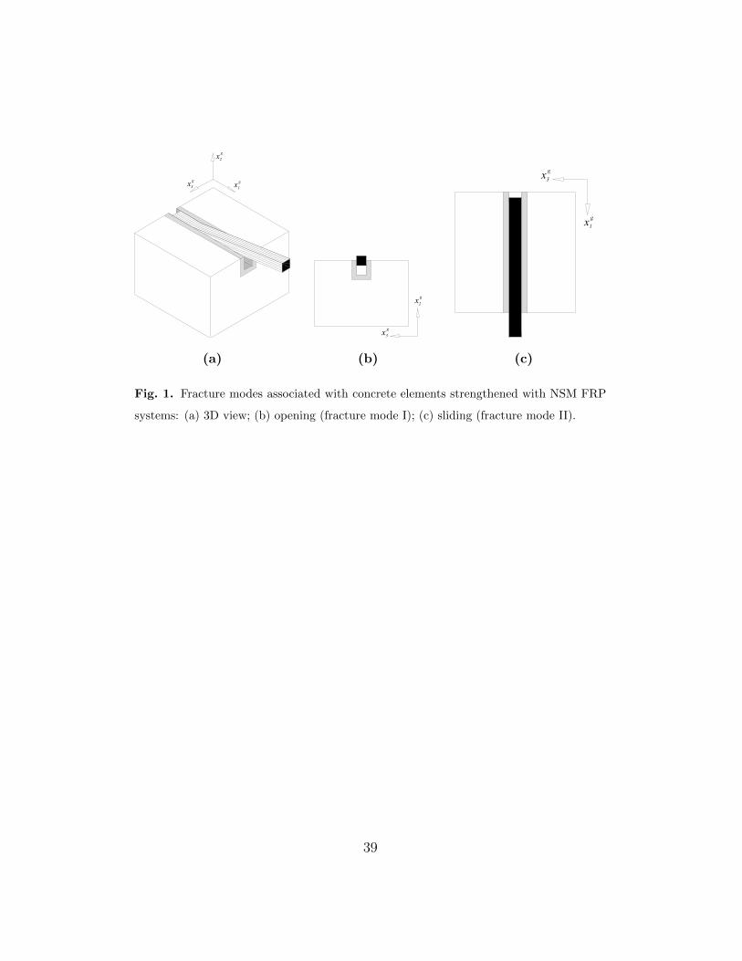
Regarding the interface’s constitutive model, it should have the ability of

describing the two possible fracture modes in concrete elements strengthened

with NSM FRP systems. Fig. 1 presents an example of a NSM FRP direct

pullout test where the FRP can be seen moving simultaneously in xg1 and xg2

directions. The sliding movement in xg1 direction is associated with fracture

mode II while the opening movement in xg2 direction is associated with mode

I.

As previously referred, most formulations used in literature are based on

adopting “a priori” analytical expressions for describing the interface bond-

6

slip law. Furthermore, these formulations are generally based on assuming

a fracture process in pure mode II and neglecting the effect of the interface

normal stresses and the occurrence of out-of-plane displacements.

The constitutive model implemented in this work was provided with sep-

arate modules which allow performing 2D and 3D analyses considering either

only mode II or both modes I and II of fracture simultaneously. This repre-

sents one of the key contributions of this work.

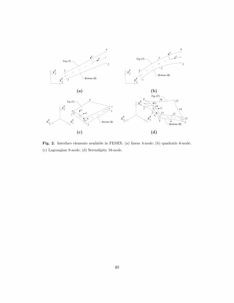
All the work presented in this paper was developed in the framework of

FEMIX 4.0 [19], which is a freeware FEM software based on the displace-

ments method. Fig. 2 presents the interface elements available in FEMIX

on which the constitutive model was implemented. Particularly, it includes

two line interface elements, with 4 and 6 nodes, which are schematically pre-

sented in Figs. 2a and 2b, respectively. Even though each of those interfaces

can be used in 2D and 3D simulations, in this work only 2D line interface

elements are addressed. FEMIX also includes two surface interface elements

with 8 and 16 nodes (Figs. 2c and 2d, respectively).

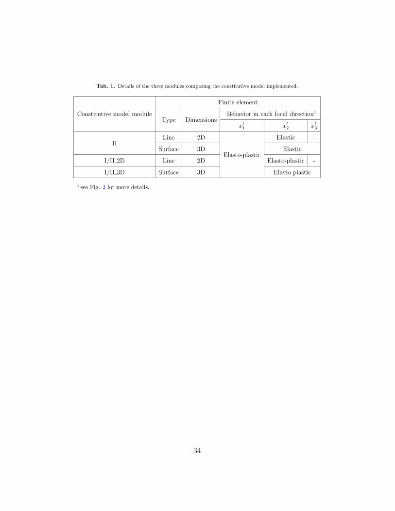
Tab. 1 presents the three modules of the implemented constitutive model:

• the first module is used for 2D and 3D FEM analyses where only frac-

ture mode II is considered (developed by Caggiano and Martinelli [20]).

Hence, the non-linear elasto-plastic behaviour is considered for local di-

rection xl1, while the remaining directions behave elastically;

• a second module was developed for 2D FEM analysis where both frac-

ture modes I and II are available (published in [21]);

• the third module addresses 3D FEM simulations where all the local

7

directions have an elasto-plastic coupled behaviour (proposed by Ca-

ballero et al. [22]).

The following section summarizes the formulation of the three modules

composing the implemented constitutive model. The most relevant expres-

sions of all modules are presented together in the Appendix A. Further de-

tailed information regarding each module should be found in [20–22].

2.1. Formulation

The constitutive model presented in this section is based on the classical

Flow Theory of Plasticity. The basic assumption of this theory, in the context

of small displacements, is the decomposition of the incremental joint relative

displacement (designated as slip from this point onwards) vector, ∆s, in an

elastic reversible part, ∆se, and a plastic irreversible one, ∆sp. The later is

defined according to a general flow rule which depends on the plastic multi-

plier ∆λ and the plastic flow direction m. Hence, the relationship between

slip and stress in the constitutive model is obtained by the following expres-

sions, where ∆σ and D are the incremental stress vector and the constitutive

matrix, respectively.

∆s = ∆se + ∆sp (1)

∆σe = De∆se = De(∆s−∆sp) (2)

∆sp = ∆λm (3)

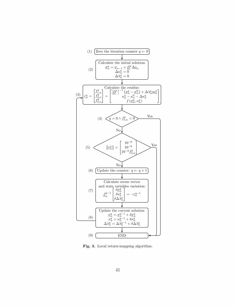
Assuming that in a generic stress state n − 1, previously converged, the

slips and stresses vectors and the hardening parameters are known, all these

8

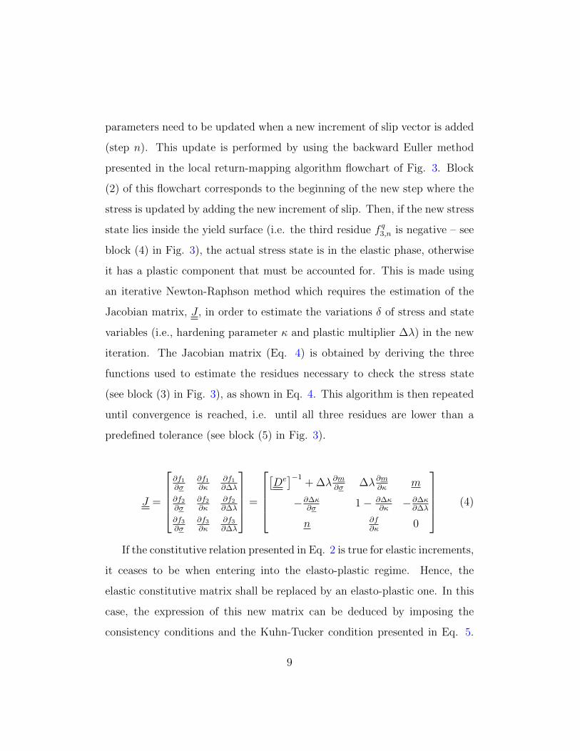
parameters need to be updated when a new increment of slip vector is added

(step n). This update is performed by using the backward Euller method

presented in the local return-mapping algorithm flowchart of Fig. 3. Block

(2) of this flowchart corresponds to the beginning of the new step where the

stress is updated by adding the new increment of slip. Then, if the new stress

state lies inside the yield surface (i.e. the third residue f q3,n is negative – see

block (4) in Fig. 3), the actual stress state is in the elastic phase, otherwise

it has a plastic component that must be accounted for. This is made using

an iterative Newton-Raphson method which requires the estimation of the

Jacobian matrix, J , in order to estimate the variations δ of stress and state

variables (i.e., hardening parameter κ and plastic multiplier ∆λ) in the new

iteration. The Jacobian matrix (Eq. 4) is obtained by deriving the three

functions used to estimate the residues necessary to check the stress state

(see block (3) in Fig. 3), as shown in Eq. 4. This algorithm is then repeated

until convergence is reached, i.e. until all three residues are lower than a

predefined tolerance (see block (5) in Fig. 3).

J =

∂f1∂σ

∂f1∂κ

∂f1∂∆λ

∂f2∂σ

∂f2∂κ

∂f2∂∆λ

∂f3∂σ

∂f3∂κ

∂f3∂∆λ

=

[De]−1

+ ∆λ∂m∂σ

∆λ∂m∂κ

m

−∂∆κ∂σ

1− ∂∆κ∂κ

−∂∆κ∂∆λ

n ∂f∂κ

0

(4)

If the constitutive relation presented in Eq. 2 is true for elastic increments,

it ceases to be when entering into the elasto-plastic regime. Hence, the

elastic constitutive matrix shall be replaced by an elasto-plastic one. In this

case, the expression of this new matrix can be deduced by imposing the

consistency conditions and the Kuhn-Tucker condition presented in Eq. 5.

9

Taking into account that the constitutive model was formulated under the

work-hardening hypotheses, this condition can be rearranged to obtain the

plastic multiplier (Eq. 6), where the parameter H is defined according to Eq.

7. Replacing the plastic multiplier in the constitutive relation of the interface

model, the elasto-plastic constitutive matrix can be obtained (Eq. 8). Hence

the new relation between slips and stresses is finally defined according Eq. 9.

∆λ ≥ 0, f(σ, κ) ≤ 0, ∆λf(σ, κ) = 0, ∆f(σ, κ) = 0 (5)

∆λ =nTDe∆s

H + nTDem(6)

H = −∂f(σ, κ)

∂λ(7)

Dep = De(1−nTDem

H + nTDem) (8)

∆σ = D∆s⇒ D =

De if loading/unloading/reloading (elastic)

Dep if loading (plastic)(9)

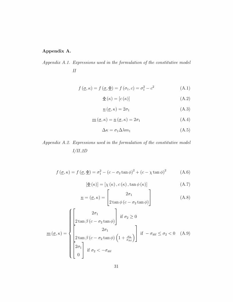
Appendix A includes all the expressions used in the formulation of the

constitutive models. This includes yield function f , hardening variables Φ,

yield surface gradient n, plastic potential g, plastic potential variables Ψ,

plastic flow direction m and hardening law ∆κ. In the following paragraphs

few important comments are presented regarding those parameters.

In all the three constitutive models (CM) the hardening parameter is the

plastic work, since, as referred before, work hardening was admitted in all

formulations. However, the way the hardening parameter affects the yield

surface is different in each CM since it depends on different variables. Hence,

in CM II there is only a single hardening variable which is the shear strength,

10

c, while in the other two CM, three variables exist: tensile (χ) and shear (c)

strengths and the friction angle (tanφ).

The plastic potential surface of CM II and I/II 2D is not explicitly de-

fined. However, since the formulation only requires the direction of the plastic

flow, that is provided instead. The major difference between these two CM

is that in CM II the plastic flow is associated while in CM I/II 2D a non-

associated flow rule is admitted. Additionally, in CM I/II 2D an additional

parameter exists which is the dilation stress, σdil. This stress corresponds

to the normal stress at which the dilatancy vanishes when compression and

shear stresses occur at the same time.

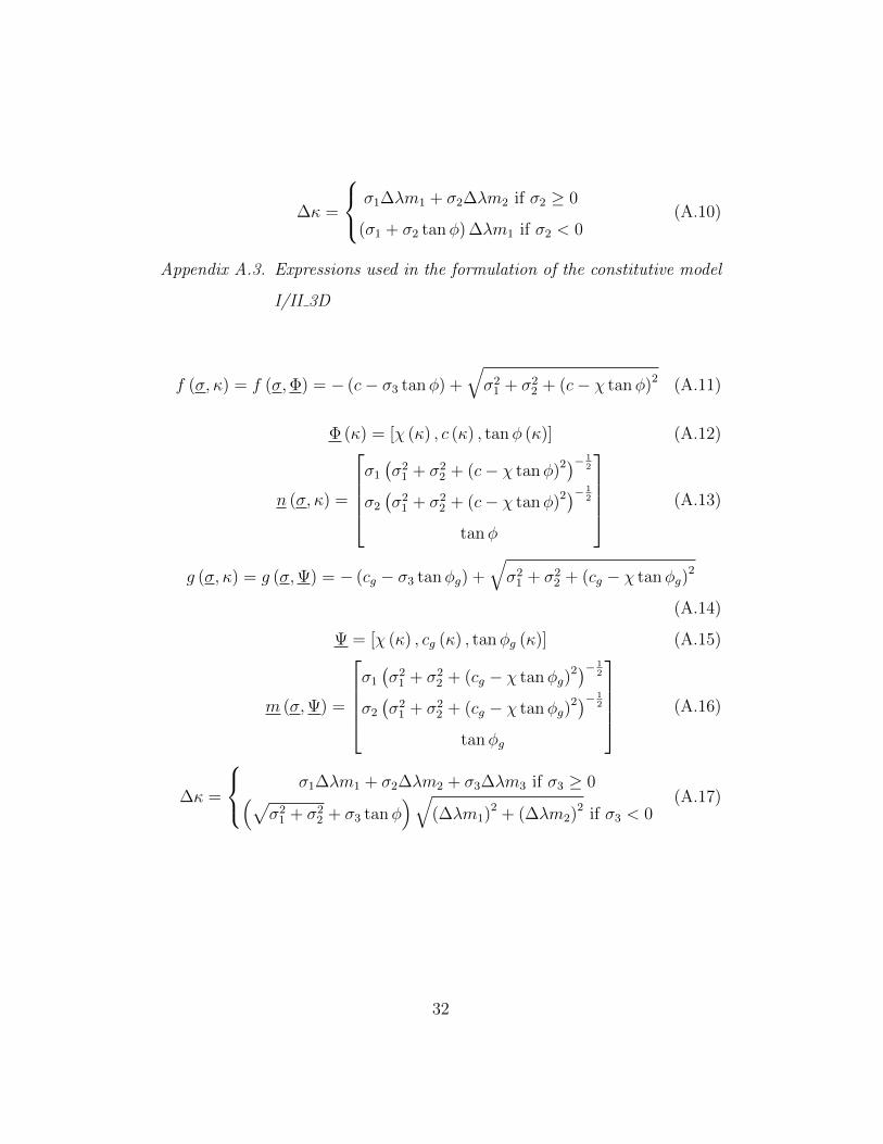
The plastic potential of CM I/II 3D is described through a hyperbola

identical to the yield surface but with different shear strength and friction

angle (tensile strength is the same). This means that, in this model, plastic

potential shear strength and friction angle need to be provided.

In terms of hardening law, it should be highlighted that, in CM I/II 2D

and CM I/II 3D, due to the different interaction that occurs between tan-

gential and normal stresses, different expressions are used for the scenarios

of tension and compression.

In all three CM, the evolution of the yield surface depends on the evo-

lution of the hardening parameters, which depend on the evolution of the

plastic work, W . The variation of the plastic work is considered by means

of a dimensionless parameter (Eq. 10), which translates the amount of frac-

ture energy, Gf , spent in a certain plastic work. Since CM I/II 2D and CM

I/II 3D account for two fracture modes, there will be two dimensionless pa-

rameters in those CM, one for fracture mode I and other for fracture mode

11

II.

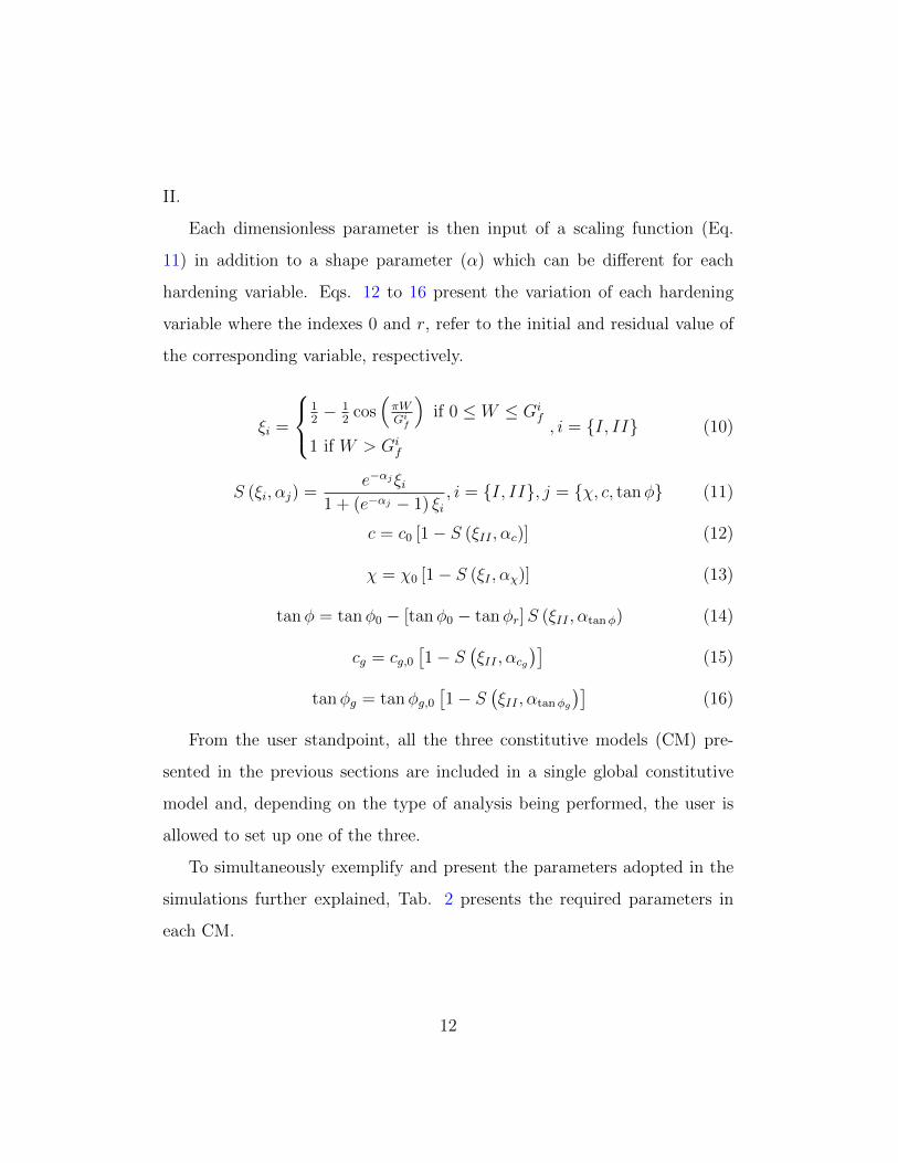
Each dimensionless parameter is then input of a scaling function (Eq.

11) in addition to a shape parameter (α) which can be different for each

hardening variable. Eqs. 12 to 16 present the variation of each hardening

variable where the indexes 0 and r, refer to the initial and residual value of

the corresponding variable, respectively.

ξi =

12− 1

2cos(πWGi

f

)if 0 ≤ W ≤ Gi

f

1 if W > Gif

, i = {I, II} (10)

S (ξi, αj) =e−αjξi

1 + (e−αj − 1) ξi, i = {I, II}, j = {χ, c, tanφ} (11)

c = c0 [1− S (ξII , αc)] (12)

χ = χ0 [1− S (ξI , αχ)] (13)

tanφ = tanφ0 − [tanφ0 − tanφr]S (ξII , αtanφ) (14)

cg = cg,0[1− S

(ξII , αcg

)](15)

tanφg = tanφg,0[1− S

(ξII , αtanφg

)](16)

From the user standpoint, all the three constitutive models (CM) pre-

sented in the previous sections are included in a single global constitutive

model and, depending on the type of analysis being performed, the user is

allowed to set up one of the three.

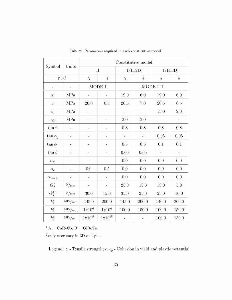
To simultaneously exemplify and present the parameters adopted in the

simulations further explained, Tab. 2 presents the required parameters in

each CM.

12

3. Model validation: outline of test setups

The implemented constitutive models were validated using experimental

results of direct pullout tests collected from the existing literature. In order

to achieve a reliable validation, two examples were selected.

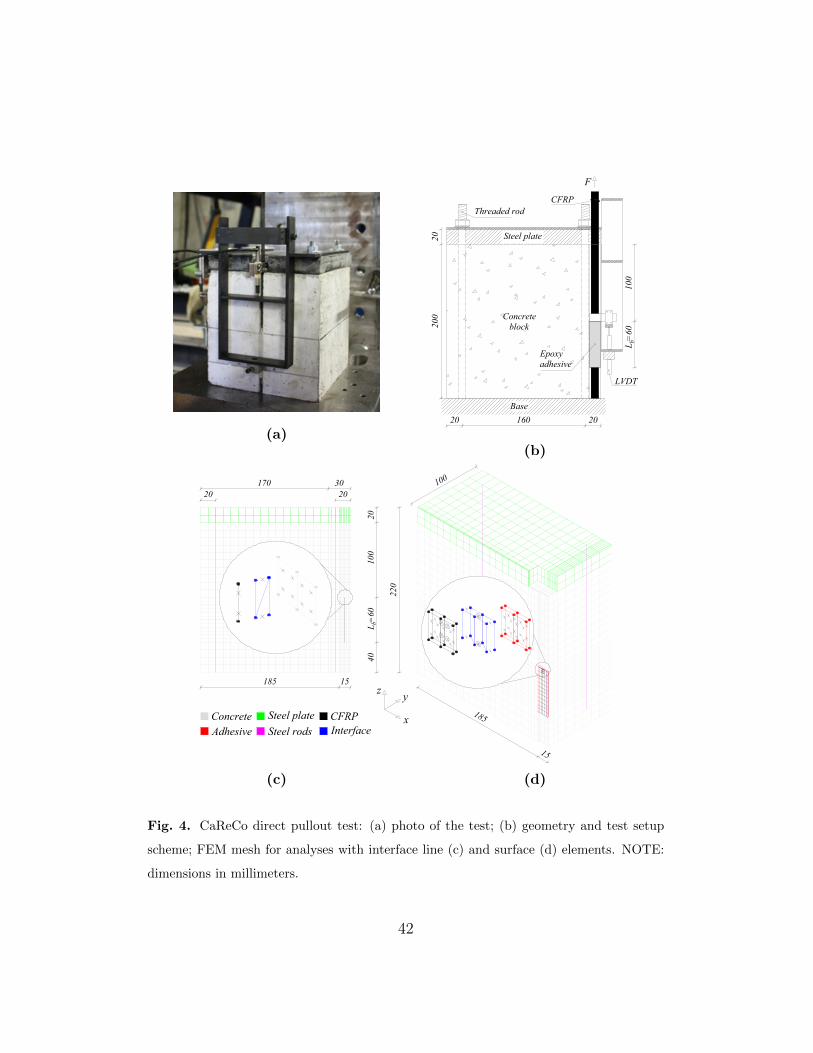
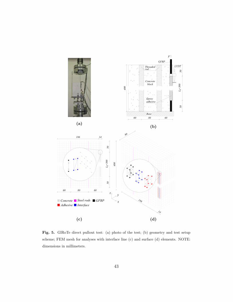
The first one, identified in this work as CaReCo, is fully described in [23]

while the second, designated as GlRoTe, is documented in [24, 25]. Figs.

4 and 5 show the geometry of the specimens and the test configurations of

CaReCo and GlRoTe tests, respectively.

While they both consist of direct pullout tests, there are interesting dif-

ferences between them, which justifies the simulation of both examples:

1. CaReCo tests uses carbon FRP (CFRP) while GlRoTe uses glass FRP

(GFRP);

2. CaReCo specimens have rectangular FRP bars while in the case of

GlRoTe round FRP bars are used;

3. CaReCo and GlRoTe adopt test configurations which induce compres-

sion and tension, respectively, in the concrete specimens used;

4. The results of CaReCo include the post-peak slip versus pullout force

curve (full range response) while the results of GlRoTe test are only up

to peak pullout force;

5. In GlRoTe test strain gauges were used on the external surface of

the GFRP along the bond length and their readings provided while

in CaReCo test such data are not available since no strain gauges were

used.

13

3.1. Details about the experiments and simulations

Each CaReCo specimen consisted of a plain concrete cube of 200 mm

edge. On the side of the specimen a groove was made and a CFRP laminate

was there inserted and fixed with an epoxy adhesive. The groove was 15 mm

deep and 5 mm wide. The CFRP laminate with a rectangular cross-section

with 1.4 mm thickness and 10 mm width was placed at the center of the

groove. GlRoTe specimens are prismatic plain concrete blocks (160x200x400

mm3) to which a GFRP round bar with 8 mm of diameter was glued with

an epoxy adhesive in a square groove with 14 mm cut on the concrete block.

To avoid premature failure of the specimen due to concrete cone formation

near the top of the block, the anchorage length was initiated at 100 mm and

50 mm from the top, in CaReCo and GlRoTe specimens, respectively. The

bond between the FRP and the concrete (Lb) was extended 60 and 300 mm

downwards, in CaReCo and GlRoTe specimens, respectively.

On top of CaReCo specimen a steel plate with 20 mm of thickness was

applied. To ensure negligible vertical displacement during the test this plate

was fixed to the base by means of four M10 threaded steel rods. A torque of

30 N.m was applied to each rod, inducing an initial state of compression in

the concrete of about 2.0 MPa.

GlRoTe specimen was fixed to the base through two M20 threaded steel

rods casted in the middle of the concrete block. Thus, in this test, both

concrete and GFRP were in tension.

Both types of test were monitored with a displacement transducer (LVDT)

and a load cell. The LVDT recorded the relative displacement at the loaded-

end between the FRP and the concrete (slip), while the applied force F

14

was recorded through the load cell. Additionally, in GlRoTe test, five strain

gauges were glued along the GFRP bar to measure its axial strains.

Based on the material characterization conducted by the authors, a mod-

ulus of elasticity of 28.4/18.6 GPa, 165/51 GPa and 7.15/10.7 GPa was ob-

tained in CaReCo/GlRoTe tests for concrete, FRP and adhesive, respectively.

Since in both types of experimental tests the specimens failed by debonding

at FRP/adhesive interface, all the non-linearity of the system was located

at that interface. Hence, all materials were assumed linear elastic using the

properties referred above (a modulus of elasticity of 200 GPa was used for

the steel elements). Additionally, the interface elements were only used at

the interface between FRP and adhesive, thus assuming that all the other

regions of contact between different materials were fully bonded.

In order to assess the performance of the implemented interface consti-

tutive model, two different FEM models were built for each type of test.

Particularly, they differ essentially in the interface elements adopted, which

were line 2D (L2D) and surface (S) interface elements.

Each FEM model was then run using either CM II or CM I/II, which

resulted in four different FEM analyses for both CaReCo and GlRoTe tests.

In the following paragraphs each single FEM model is described in detail.

The parameters adopted in each constitutive model are presented in Tab. 2.

3.2. FEM model with L2D elements

In L2D FEM model, the direct pullout tests were modelled as a plane

stress problem using the meshes represented in Fig. 4c and 5c for CaReCo

and GlRoTe specimens, respectively. For for both specimens the type of ele-

ments used was the same, namely: 4-node Serendipity plane stress elements

15

with 2 × 2 Gauss-Legendre integration scheme for both concrete block and

steel plate; 2-node frame 2D elements for both FRP bars and steel rods;

4-node interface L2D elements (see Fig. 2a) with 2× 1 Gauss-Lobatto inte-

gration scheme.

Both types of specimens were fixed to the corresponding testing machine

by means of steel threaded rods. The only difference between them is that,

while in the case of GlRoTe the rods were directly in contact with the concrete

block, in CaReCo they were connected to a steel plate which in turn was

in contact with the concrete block. Thus, the FEM support conditions in

both types of tests consisted in fixing the bottom node of the steel rods.

Additionally, unilateral contact supports were applied at the concrete block’s

base. Those restrain the downward movement in z direction (see Figs. 4 and

5), but allow upward free movement. In CaReCo test, the effect of the

pre-stress in the steel rods was simulated by applying a uniform temperature

variation to the rod elements equivalent to the torque applied.

In both tests the load was applied by means of a vertical prescribed

displacement (direction z – see Figs. 4 and 5) in the top node of the FRP

element.

3.3. FEM model with S elements

The S FEM model outlined in this section was built in order to test the

S elements, thus deals with a 3D analysis with solid elements (see Figs. 4d

4d). Due to computational costs, in each case only half of the specimen was

modelled since both specimens have a symmetry on the xz plan.

In both CaReCo and GlRoTe concrete block specimens, steel plate (in

the case of CaReCo), adhesive and FRP were modelled using 8-node solid

16

elements with 2 × 2 × 2 Gauss-Legendre integration scheme. For the steel

rods 2-node frame 3D elements were adopted. The interface elements were

modelled with 8-node interface S elements (see Fig. 2c) and 2 × 2 Gauss-

Lobatto integration scheme.

The test boundary conditions were simulated in a way similar to that

explained in the previous section. Additionally, in these 3D simulations the

displacements following y axis were also restrained along the symmetry plan.

The load was also applied by means of a vertical prescribed displacement,

in this case, in all the top nodes of the FRP.

3.4. Parameters of each interface constitutive model

While in the analyses with CM II both L2D and S FEM models used

the same input parameters for the interface constitutive model, in CM I/II

simulations the parameters used by each FEM model (2D and 3D) were

slightly different as shown in Tab. 2.

These differences in the parameters used in each simulation with CM I/II

are related to the influence that the behaviour in the normal direction has in

the global response. In fact, the behaviour in the normal direction of FEM

model with S elements is affected by the stiffness of the surrounding materials

(adhesive and concrete) which can be seen as a “confinement” effect in the

normal direction. Such influence does not exist when CM II is used since the

behaviour in the normal direction is considered elastic in both L2D and S

FEM models.

4. Model validation: numerical results

17

As previously referred, only CaReCo test results include the post-peak

response while only GlRoTe test results provide FRP strains. Hence, for the

sake of brevity, in the following sections the obtained results are presented

and discussed only for CaReCo test. The only exceptions to this are related

with the global response in terms of pullout force versus slip and the obtained

FRP strains. The former is discussed for both (CaReCo and GlRoTe) in

order to show the success of the FEM simulations. The later is presented

and analyzed in Section 4.4 for GlRoTe test only. Nevertheless it is worth

to highlight that the trends and conclusions drawn in the following sections

were very similar in the FEM simulation of both types of tests, thus are valid

for both.

4.1. Experimental versus numerical results

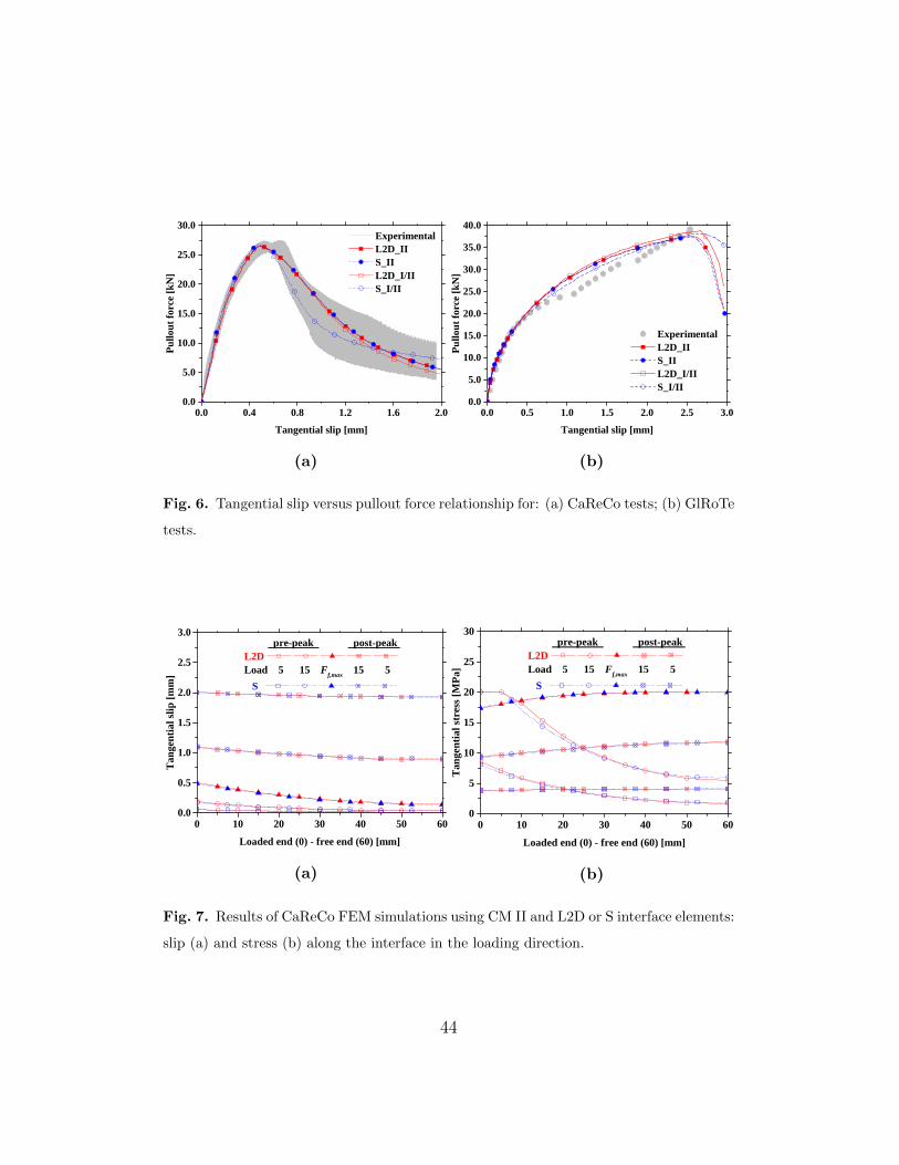
Figs. 6a and 6b present the results of all the eight FEM analyses con-

ducted, in terms of the relationship between pullout force and slip at the

loaded-end. Each graph includes the experimental results envelope and the

results for the FEM analyses with L2D and S interface elements, as well as

using both CM II and CM I/II.

For both types of test, in the case of L2D FEM models, the pullout force

was taken from the top node of the FRP element (the node with imposed

displacement) while the slip was taken from the top integration point of the

top line interface element (see Figs. 4c and 5c). In the case of S FEM models,

the pullout force was computed as the sum of all the forces obtained in all

top nodes of the FRP element (loaded nodes), while the slip was obtained

from one of the top nodes of the top surface elements (see Fig. 4d and 5d).

18

All the FEM analyses of CaReCo test successfully captured the three

major stages of the experimental tests:

• the initial stage, governed by the chemical bond between concrete, ad-

hesive and CFRP. Typically this stage is characterized by an almost

linear behavior;

• the second stage, corresponding to the system’s stiffness degradation

that occurs as a consequence of the progressive loss of chemical bond;

• the third stage (post-peak branch), governed by the friction that exist

between the CFRP laminate and the surrounding adhesive.

The most remarkable aspect is related with the FEM model using inter-

face S elements and considering both fracture modes (CM I/II). This is the

FEM model which better captured the abrupt force decrease at the beginning

of the post-peak branch. This, once again, highlights the three dimensional

nature of the NSM FRP technique and the need for conducting 3D FEM

analyses.

In GlRoTe, since the post-peak response was not registered, only the first

two stages mentioned above were obtained. The FEM results were found to

be very accurate in the first stage (up to a load level of 15-20 kN) as well as

in terms of maximum pullout force prediction. Contrarily, the results in the

middle region of the pullout force versus slip curve were not as accurate. The

authors believe that this inaccuracy should be associated with acquisition

difficulties during the experimental tests.

In addition, for GlRoTe test the beginning of the post-peak FEM curves

19

is also included. This suggests a sudden pullout force decrease which can

also justify the difficulty in capturing the post-peak response experimentally.

4.2. CM II versus CM I/II results

Figs. 7 and 8 present the graphs with the evolution of interface’s slips

and stresses in the simulations with both L2D and S FEM models using CM

II and CM I/II, respectively. In all curves the horizontal axis corresponds

to the 60 mm bonded length. For the sake of readability, the graphs only

include two curves in the pre-peak phase for load levels of 5 and 15 kN, the

curve for the peak load (Ffmax) and two curves in the two post-peak phase

for load levels of 15 and 5 kN.

In the FEM models with L2D interfaces, slips and stresses were monitored

at the integration points of the L2D interface elements which coordinates

coincide with those of the interfaces’ nodes.

In order to get, for each parameter, a curve comparable to that obtained

in the models with L2D interfaces, in FEM models with surface elements,

slips and stresses were read at the middle integration points of the two mid-

dle columns of surface interface elements. The referred reading points are

inscribed inside circles in Fig. 4d.

Considering that there are differences in terms of numerical integration

between 2D and 3D FEM models, the first conclusion that can be taken is

that the results when using CM II are practically the same for both L2D and

S FEM models, while they present some differences when using CM I/II.

In fact, while in the FEM models using CM II the curves for L2D and S

seem to be just slightly shifted (as a consequence of the referred differences

in the numerical integration), in the FEM models using CM I/II they are

20

actually different in terms of shape. This corroborates the previously referred

influence of the normal direction behavior.

Another conclusion that can be drawn is related with the curves of the

parameters in the normal direction. Those are only presented for the FEM

models using CM I/II and show that, when using L2D interface elements

there is normal slip while when using S interface elements the normal slip

is almost zero. As a consequence, the opposite occurs in terms of normal

stress, i.e. when using L2D the normal stress is almost zero while when

using S compressions are obtained in the normal direction. These findings

corroborate the “confinement” effect that only exist in 3D simulations due to

the influence of the surrounding materials stiffness, as previously mentioned

(see section 3.4).

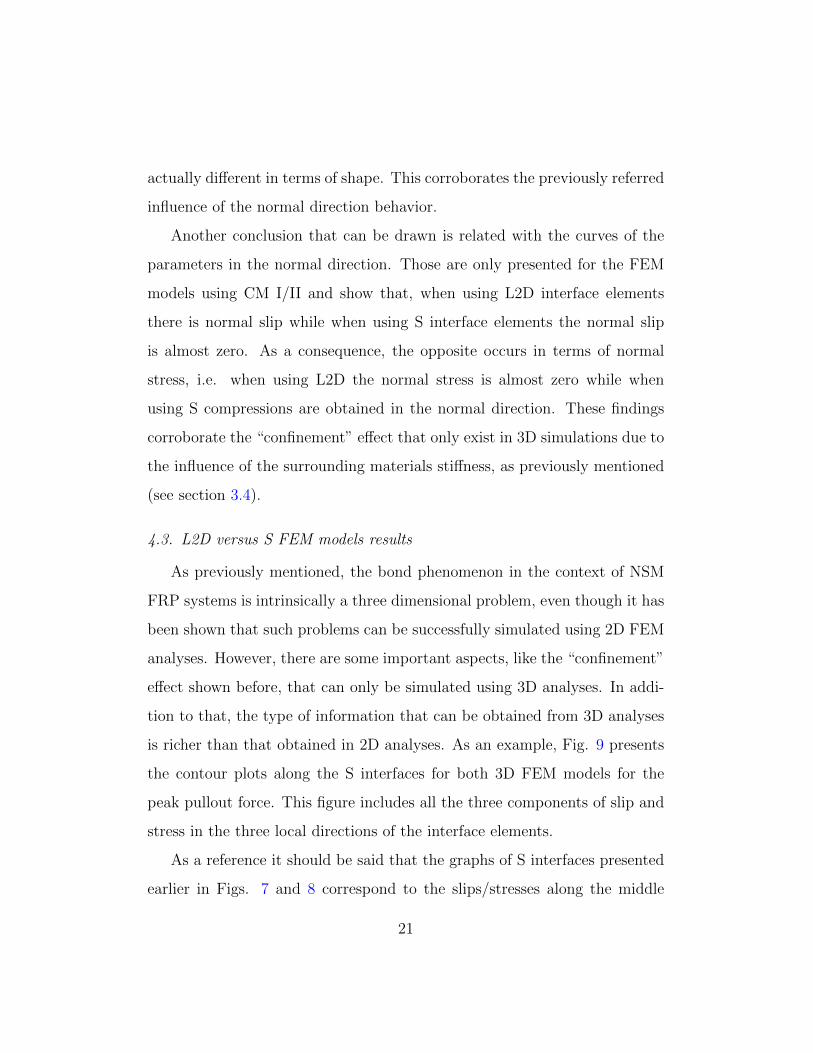
4.3. L2D versus S FEM models results

As previously mentioned, the bond phenomenon in the context of NSM

FRP systems is intrinsically a three dimensional problem, even though it has

been shown that such problems can be successfully simulated using 2D FEM

analyses. However, there are some important aspects, like the “confinement”

effect shown before, that can only be simulated using 3D analyses. In addi-

tion to that, the type of information that can be obtained from 3D analyses

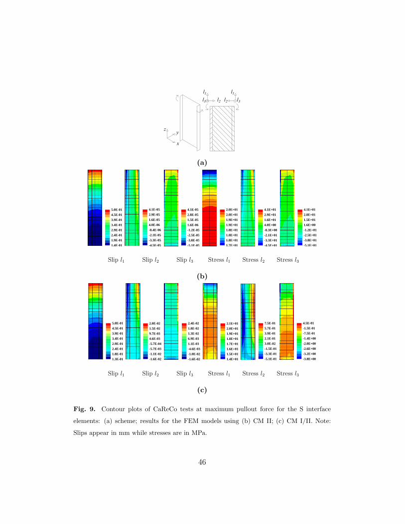
is richer than that obtained in 2D analyses. As an example, Fig. 9 presents

the contour plots along the S interfaces for both 3D FEM models for the

peak pullout force. This figure includes all the three components of slip and

stress in the three local directions of the interface elements.

As a reference it should be said that the graphs of S interfaces presented

earlier in Figs. 7 and 8 correspond to the slips/stresses along the middle

21

vertical line in each plot of Fig. 9, which coincides with the location of

the CFRP and L2D interfaces in the 2D models. Now, a global picture of

what happens along the entire perimeter of the interface between CFRP and

adhesive can also be seen.

Firstly, this figure shows that the effect of the eccentric location of the

CFRP laminate is well captured by means of the interface-based modeling.

For example, the slips in l1 direction (first plot in both Figs. 9b and 9c) are

slightly larger in the left side than in the right side, which correspond to inner

and outer sides of the bond, respectively. This effect should be associated

with the downwards movement of the concrete block as the CFRP is being

pulled upwards, which should be smaller closer to the concrete block outer

face.

Secondly it shows the different behavior obtained when using CM I and

I/II. This is more evident in the stresses along l1 direction (fourth plot in

both Figs. 9b and 9c). This plots show that due to the elastic behavior in the

remaining direction when using CM II, the l1 stresses are similar in all the

three sides of the groove that were simulated. Contrarily, when using CM I/II

the behavior in all the three sides is quite different. In fact, comparing the

region closer to the loaded end of each groove side, values of approximately

14, 16 and 18 MPa of tangential stress can be found, at maximum pullout

force, for the outer, middle and inner sides of the groove, respectively. This

numerical observation can be explained by the curvature that occurs at the

CFRP during the pullout. This further highlights again the different loading

stage of each region of the interface. In addition, with these plots, it is easy

to identify the regions where the interface remains in the elastic range and

22

those where it already entered the softening stage.

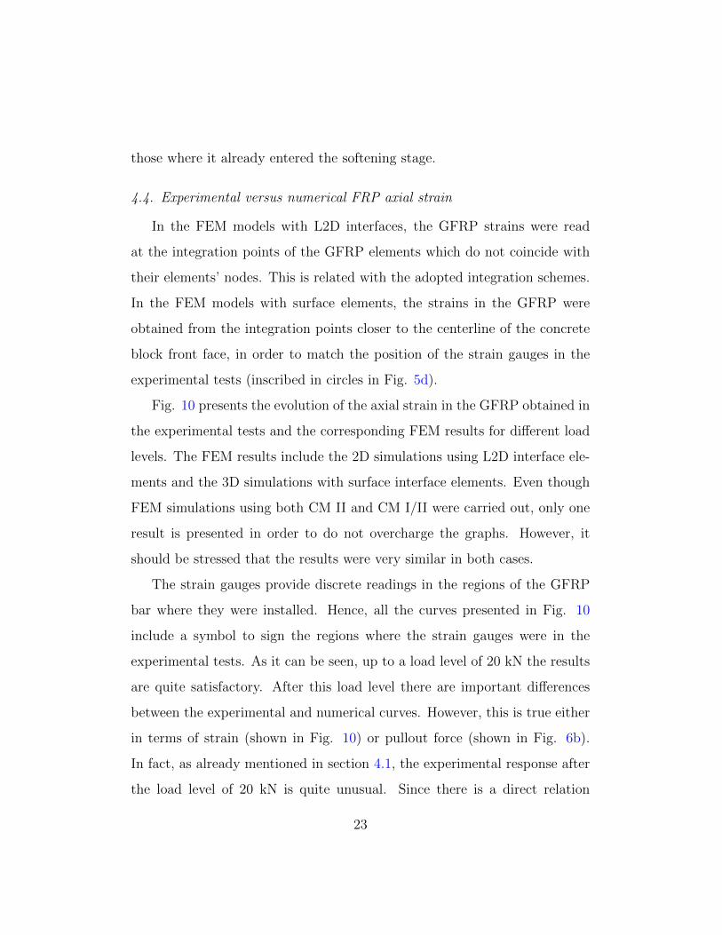
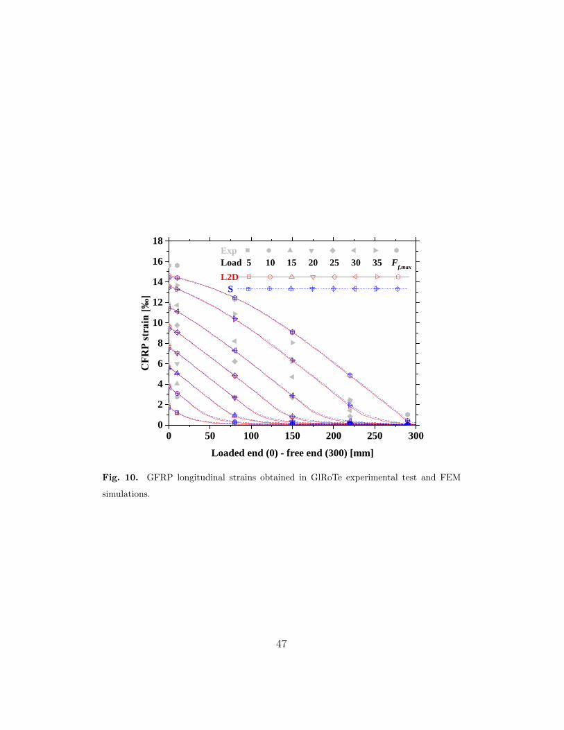
4.4. Experimental versus numerical FRP axial strain

In the FEM models with L2D interfaces, the GFRP strains were read

at the integration points of the GFRP elements which do not coincide with

their elements’ nodes. This is related with the adopted integration schemes.

In the FEM models with surface elements, the strains in the GFRP were

obtained from the integration points closer to the centerline of the concrete

block front face, in order to match the position of the strain gauges in the

experimental tests (inscribed in circles in Fig. 5d).

Fig. 10 presents the evolution of the axial strain in the GFRP obtained in

the experimental tests and the corresponding FEM results for different load

levels. The FEM results include the 2D simulations using L2D interface ele-

ments and the 3D simulations with surface interface elements. Even though

FEM simulations using both CM II and CM I/II were carried out, only one

result is presented in order to do not overcharge the graphs. However, it

should be stressed that the results were very similar in both cases.

The strain gauges provide discrete readings in the regions of the GFRP

bar where they were installed. Hence, all the curves presented in Fig. 10

include a symbol to sign the regions where the strain gauges were in the

experimental tests. As it can be seen, up to a load level of 20 kN the results

are quite satisfactory. After this load level there are important differences

between the experimental and numerical curves. However, this is true either

in terms of strain (shown in Fig. 10) or pullout force (shown in Fig. 6b).

In fact, as already mentioned in section 4.1, the experimental response after

the load level of 20 kN is quite unusual. Since there is a direct relation

23

between GFRP strain and pullout force, if the later is not well captured, the

former will not be well captured as well. At the peak pullout force, again the

numerical model captured very well the results obtained in the experimental

test.

5. Conclusions

In this work, the major details about the implementation of an interface

constitutive model (CM) in the FEMIX software were presented. It shall be

emphasized that this CM is an adaptation of three already existing CM for

quasi-brittle materials. One of the CM only allows for accounting fracture

mode II while the other two CM deal with considering both fractures modes

I and II in 2D or 3D FEM simulations.

Hence, the main contributions of this paper were, in the first place, bring

those three CM to the field of NSM FRP systems’ interfaces simulation. Sec-

ondly, implementing the three CM as a single CM in order to made available

in FEMIX a single and complete interface model. The third contribution cor-

responds to the presentation of FEM simulations with the developed model,

thus highlighting its validation.

The later contribution is specially important, since this work adds to the

literature examples of 2D and 3D FEM simulations of pullout bond tests,

either using only mode II of fracture or combining both modes I and II

together. Additionally, it was shown that the implemented model can be

used with line or surface interface elements in the framework of the well-

known discrete crack analysis.

Regarding the results of the performed simulations, a good agreement

24

between the experimental results and the numerical ones was found in all

simulations performed in terms of pullout force versus slip. In addition,

it was shown that further and more detailed information can be obtained

when using surface interface elements. Namely, the effect of the eccentric

location of the FRP bar is well captured by means of the 3D FEM simulations

performed. The use of surface interfaces with CM I/II also allowed to verify

that the bond behavior varies, not only in the FRP tangential direction (load

direction) but also in its normal direction (perpendicular to the loading). In

fact, the value of maximum tangential stress varies from the outer to the

inner regions of the interface FRP/adhesive.

Finally, a comparison was made in terms of FRP axial strains where good

agreement between experimental and numerical values was also obtained.

Acknowledgments

This work was supported by FEDER funds through the Operational Pro-

gram for Competitiveness Factors – COMPETE and National Funds through

FCT (Portuguese Foundation for Science and Technology) under the project

CutInDur FCOMP-01-0124-FEDER-014811 (ref. PTDC/ECM/112396/2009)

and partly financed by the project POCI-01-0145-FEDER-007633. The first

author wishes also to acknowledge the Grant No. SFRH/BD/87443/2012

provided by FCT and the mobility grant provided by the “EnCoRe” Project

(FP7-PEOPLE-2011-IRSES no.295283; www.encore-fp7.unisa.it) funded by

the European Union within the Seventh Framework Programme.

25

References

[1] Bakis C, Bank L, Brown V, Cosenza E, Davalos J, Lesko J, et al. Fiber-

reinforced polymer composites for construction – state-of-the-art review.

Journal of Composites for Construction 2002;6(2):73–87. URL http:

//dx.doi.org/10.1061/(asce)1090-0268(2002)6:2(73).

[2] Coelho M, Sena-Cruz J, Neves L. A review on the bond behavior of

FRP NSM systems in concrete. Construction and Building Materials

2015;93:1157–69. URL http://dx.doi.org/10.1016/j.conbuildmat.

2015.05.010.

[3] Sena-Cruz J, Barros J, Azevedo A. Elasto plastic multi fixed smeared

crack model for concrete. Tech. Rep. 04-DEC/E-05; Civil Engineering

Department, University of Minho, Guimaraes, Portugal; 2004.

[4] Ventura A, Barros J, Azevedo A, Sena-Cruz J. Multi-fixed smeared

3d crack model to simulate the behavior of fiber reinforced concrete

structures. In: CCC2008 – Challenges for Civil Construction, FEUP,

Porto, Portugal. 2008,.

[5] Caggiano A, Etse G, Martinelli E. Interface model for fracture behaviour

of fiber-reinforced cementitious composites (FRCCs). European Journal

of Environmental and Civil Engineering 2011;15(9):1339–59. URL http:

//dx.doi.org/10.1080/19648189.2011.9714858.

[6] Ceroni F, Pecce M, Bilotta A, Nigro E. Bond behavior of FRP

NSM systems in concrete elements. Composites Part B: Engi-

26

neering 2012;43(2):99–109. URL http://dx.doi.org/10.1016/j.

compositesb.2011.10.017.

[7] Novidis D, Pantazopoulou SJ, Tentolouris E. Experimental study

of bond of NSM-FRP reinforcement. Construction and Building

Materials 2007;21(8):1760–70. URL http://dx.doi.org/10.1016/j.

conbuildmat.2006.05.054.

[8] Capozucca R. Analysis of bond-slip effects in RC beams strengthened

with NSM CFRP rods. Composite Structures 2013;102:110–23. URL

http://dx.doi.org/10.1016/j.compstruct.2013.02.024.

[9] Mohamed Ali MS, Oehlers DJ, Griffith MC, Seracino R. Interfacial

stress transfer of near surface-mounted frp-to-concrete joints. Engineer-

ing Structures 2008;30(7):1861–8. URL http://dx.doi.org/10.1016/

j.engstruct.2007.12.006.

[10] Martinelli E, Caggiano A. A unified theoretical model for the mono-

tonic and cyclic response of FRP strips glued to concrete. Polymers

2014;6(2):370–81. URL http://dx.doi.org/10.3390/polym6020370.

[11] Sena-Cruz J, Barros J, Gettu R, Azevedo A. Bond behavior of near-

surface mounted CFRP laminate strips under monotonic and cyclic load-

ing. Journal of Composites for Construction 2006;10(4):295–303. URL

http://dx.doi.org/10.1061/(ASCE)1090-0268(2006)10:4(295).

[12] Ceroni F, Barros J, Pecce M, Ianniciello M. Assessment of nonlinear

bond laws for near-surface-mounted systems in concrete elements. Com-

27

posites Part B: Engineering 2013;45(1):666–81. URL http://dx.doi.

org/10.1016/j.compositesb.2012.07.006.

[13] Sharaky IA, Barros JAO, Torres L. FEM-based modelling of NSM-FRP

bond behaviour. In: FRPRCS-11, Guimaraes, Portugal. 2013,.

[14] Echeverria M, Perera R. Three dimensional nonlinear model of beam

tests for bond of near-surface mounted FRP rods in concrete. Compos-

ites Part B: Engineering 2013;54:112–24. URL http://dx.doi.org/10.

1016/j.compositesb.2013.05.008.

[15] De Lorenzis L, Lundgren K, Rizzo A. Anchorage length of near-surface

mounted fiber-reinforced polymer bars for concrete strengthening – ex-

perimental investigation and numerical modeling. ACI Structural Jour-

nal 2004;101(2):269–78. URL http://dx.doi.org/10.14359/13025.

[16] Sasmal S, Khatri CP, Ramanjaneyulu K, Srinivas V. Numeri-

cal evaluation of bond-slip relations for near-surface mounted car-

bon fiber bars embedded in concrete. Construction and Building

Materials 2013;40:1097–109. URL http://dx.doi.org/10.1016/j.

conbuildmat.2012.11.073.

[17] Teng JG, Zhang SS, Dai JG, Chen JF. Three-dimensional meso-scale

finite element modeling of bonded joints between a near-surface mounted

FRP strip and concrete. Computers & Structures 2013;117:105–17. URL

http://dx.doi.org/10.1016/j.compstruc.2012.12.002.

[18] Lundqvist J, Nordin H, Taljsten B, Olofsson T. Numerical analysis of

concrete beams strengthened with CFRP – a study of anchorage lengths.

28

In: International Symposium on Bond Behaviour of FRP in Structures

(BBFS2005), Hong Kong, China. 2005, p. 247–54.

[19] Sena-Cruz J, Barros J, Azevedo A, Gouveia A. Numerical simulation

of the nonlinear behavior of RC beams strengthened with NSM CFRP

strips. In: CNME 2007-Congress on Numerical Methods in Engineering

and XXVIII CILAMCE – Iberian Latin American Congress on Compu-

tational Methods in Engineering, FEUP, Porto, Portugal. 2007,.

[20] Caggiano A, Martinelli E. A fracture-based interface model for simu-

lating the bond behaviour of FRP strips glued to a brittle substrate.

Composite Structures 2013;99:397–403. URL http://dx.doi.org/10.

1016/j.compstruct.2012.12.011.

[21] Caggiano A, Martinelli E. Fracture-based model for mixed mode crack-

ing of FRP strips glued on concrete. In: Bond in Concrete 2012, Brescia,

Italy. 2012,.

[22] Caballero A, Willam KJ, Carol I. Consistent tangent formulation for

3d interface modeling of cracking/fracture in quasi-brittle materials.

Computer Methods in Applied Mechanics and Engineering 2008;197(33-

40):2804–22. URL http://dx.doi.org/10.1016/j.cma.2008.01.011.

[23] Fernandes P, Silva P, Sena-Cruz J. Bond and flexural behavior of

concrete elements strengthened with NSM CFRP laminate strips un-

der fatigue loading. Engineering Structures 2015;84:350–61. URL

http://dx.doi.org/10.1016/j.engstruct.2014.11.039.

29

[24] Bilotta A, Ceroni F, Di Ludovico M, Nigro E, Pecce M, Man-

fredi G. Bond efficiency of EBR and NSM FRP systems for

strengthening concrete members. Journal of Composites for Construc-

tion 2011;15(5):757–72. URL http://dx.doi.org/10.1061/(asce)cc.

1943-5614.0000204.

[25] Bilotta A, Ceroni F, Barros J, Costa I, Palmieri A, Szab Z, et al. Bond

of NSM FRP-strengthened concrete: round robin test initiative. Journal

of Composites for Construction 2016;20(1). URL http://dx.doi.org/

10.1061/(ASCE)CC.1943-5614.0000579.

30

Appendix A.

Appendix A.1. Expressions used in the formulation of the constitutive model

II

f (σ, κ) = f (σ,Φ) = f (σ1, c) = σ21 − c2 (A.1)

Φ (κ) = [c (κ)] (A.2)

n (σ, κ) = 2σ1 (A.3)

m (σ, κ) = n (σ, κ) = 2σ1 (A.4)

∆κ = σ1∆λm1 (A.5)

Appendix A.2. Expressions used in the formulation of the constitutive model

I/II 2D

f (σ, κ) = f (σ,Φ) = σ21 − (c− σ2 tanφ)2 + (c− χ tanφ)2 (A.6)

[Φ (κ)] = [χ (κ) , c (κ) , tanφ (κ)] (A.7)

n = (σ, κ) =

2σ1

2 tanφ (c− σ2 tanφ)

(A.8)

m (σ, κ) =

2σ1

2 tan β (c− σ2 tanφ)

if σ2 ≥ 0

2σ1

2 tan β (c− σ2 tanφ)(

1 + σ2σdil

) if − σdil ≤ σ2 < 0

2σ1

0

if σ2 < −σdil

(A.9)

31

∆κ =

σ1∆λm1 + σ2∆λm2 if σ2 ≥ 0

(σ1 + σ2 tanφ) ∆λm1 if σ2 < 0(A.10)

Appendix A.3. Expressions used in the formulation of the constitutive model

I/II 3D

f (σ, κ) = f (σ,Φ) = − (c− σ3 tanφ) +

√σ2

1 + σ22 + (c− χ tanφ)2 (A.11)

Φ (κ) = [χ (κ) , c (κ) , tanφ (κ)] (A.12)

n (σ, κ) =

σ1

(σ2

1 + σ22 + (c− χ tanφ)2)− 1

2

σ2

(σ2

1 + σ22 + (c− χ tanφ)2)− 1

2

tanφ

(A.13)

g (σ, κ) = g (σ,Ψ) = − (cg − σ3 tanφg) +

√σ2

1 + σ22 + (cg − χ tanφg)

2

(A.14)

Ψ = [χ (κ) , cg (κ) , tanφg (κ)] (A.15)

m (σ,Ψ) =

σ1

(σ2

1 + σ22 + (cg − χ tanφg)

2)− 12

σ2

(σ2

1 + σ22 + (cg − χ tanφg)

2)− 12

tanφg

(A.16)

∆κ =

σ1∆λm1 + σ2∆λm2 + σ3∆λm3 if σ3 ≥ 0(√σ2

1 + σ22 + σ3 tanφ

)√(∆λm1)2 + (∆λm2)2 if σ3 < 0

(A.17)

32

List of Tables

1 Details of the three modules composing the constitutive model

implemented. . . . . . . . . . . . . . . . . . . . . . . . . . . . 34

2 Parameters required in each constitutive model. . . . . . . . . 35

33

Tab. 1. Details of the three modules composing the constitutive model implemented.

Constitutive model module

Finite element

Type DimensionsBehavior in each local direction1

xl1 xl2 xl3

IILine 2D

Elasto-plastic

Elastic -

Surface 3D Elastic

I/II 2D Line 2D Elasto-plastic -

I/II 3D Surface 3D Elasto-plastic

1 see Fig. 2 for more details.

34

Tab. 2. Parameters required in each constitutive model.

Symbol UnitsConstitutive model

II I/II 2D I/II 3D

Test1 A B A B A B

- - MODE II MODE I II

χ MPa - - 19.0 6.0 19.0 6.0

c MPa 20.0 6.5 20.5 7.0 20.5 6.5

cg MPa - - - - 15.0 2.0

σdil MPa - - 2.0 2.0 - -

tanφ - - - 0.8 0.8 0.8 0.8

tanφg - - - - - 0.05 0.05

tanφr - - - 0.5 0.5 0.1 0.1

tan β - - - 0.05 0.05 - -

αχ - - - 0.0 0.0 0.0 0.0

αc - 0.0 0.5 0.0 0.0 0.0 0.0

αtanφ - - - 0.0 0.0 0.0 0.0

GIf

N/mm - - 25.0 15.0 15.0 5.0

GIIf

N/mm 30.0 15.0 35.0 25.0 25.0 10.0

ke1 MPa/mm 145.0 200.0 145.0 200.0 140.0 200.0

ke2 MPa/mm 1x106 1x106 100.0 150.0 100.0 150.0

ke3 MPa/mm 1x1062 1x1062 - - 100.0 150.0

1 A = CaReCo, B = GlRoTe.

2 only necessary in 3D analysis.

Legend: χ - Tensile strength; c, cg - Cohesion in yield and plastic potential

35

functions, respectively; σdil - Normal stress at which the dilatancy vanishes;

tanφ, tanφg - Friction angle in yield and plastic potential functions, respec-

tively; tanφr - Residual friction angle; tan β - Dilation angle; αχ, αc, αtanφ

- Tensile strength, cohesion and friction angle softening parameters, respec-

tively; GIf , G

IIf - Fracture energy in modes I and II, respectively; ke1, ke2, ke3 -

Elastic tangential stiffness in l1, l2 and l3 local directions, respectively.

36

List of Figures

1 Fracture modes associated with concrete elements strength-

ened with NSM FRP systems: (a) 3D view; (b) opening (frac-

ture mode I); (c) sliding (fracture mode II). . . . . . . . . . . 39

2 Interface elements available in FEMIX: (a) linear 4-node; (b)

quadratic 6-node; (c) Lagrangian 8-node; (d) Serendipity 16-

node. . . . . . . . . . . . . . . . . . . . . . . . . . . . . . . . . 40

3 Local return-mapping algorithm. . . . . . . . . . . . . . . . . 41

4 CaReCo direct pullout test: (a) photo of the test; (b) ge-

ometry and test setup scheme; FEM mesh for analyses with

interface line (c) and surface (d) elements. NOTE: dimensions

in millimeters. . . . . . . . . . . . . . . . . . . . . . . . . . . . 42

5 GlRoTe direct pullout test: (a) photo of the test; (b) geometry

and test setup scheme; FEM mesh for analyses with interface

line (c) and surface (d) elements. NOTE: dimensions in mil-

limeters. . . . . . . . . . . . . . . . . . . . . . . . . . . . . . . 43

6 Tangential slip versus pullout force relationship for: (a) CaReCo

tests; (b) GlRoTe tests. . . . . . . . . . . . . . . . . . . . . . . 44

7 Results of CaReCo FEM simulations using CM II and L2D or

S interface elements: slip (a) and stress (b) along the interface

in the loading direction. . . . . . . . . . . . . . . . . . . . . . 44

8 Results of CaReCo FEM simulations using CM I/II and L2D

or S interface elements: slip (a) and stress (b) along the inter-

face in the loading direction; slip (c) and stress (d) along the

interface in the normal direction. . . . . . . . . . . . . . . . . 45

37

9 Contour plots of CaReCo tests at maximum pullout force for

the S interface elements: (a) scheme; results for the FEM

models using (b) CM II; (c) CM I/II. Note: Slips appear in

mm while stresses are in MPa. . . . . . . . . . . . . . . . . . . 46

10 GFRP longitudinal strains obtained in GlRoTe experimental

test and FEM simulations. . . . . . . . . . . . . . . . . . . . . 47

38

x g1

x g2

x g3

(a)

x g2

x g3

(b)

x g3

x g1

(c)

Fig. 1. Fracture modes associated with concrete elements strengthened with NSM FRP

systems: (a) 3D view; (b) opening (fracture mode I); (c) sliding (fracture mode II).

39

Bottom (B)1

3

2x

2

4

Top (T)

2xg

1xg

l

1x l

(a)

1

23

6

5

4

Top (T)

Bottom (B)2xg

1x l2x l

1xg

(b)

2xg

1xg3xg

2

37

8

615

Top (T)

Bottom (B)

2xl

1xl

3xl

(c)

2xg

1xg3xg

12

3

11

10

12

4 513

14

15169Top (T)

Bottom (B)

2xl

1xl

3xl

(d)

Fig. 2. Interface elements available in FEMIX: (a) linear 4-node; (b) quadratic 6-node;

(c) Lagrangian 8-node; (d) Serendipity 16-node.

40

Zero the iteration counter q ← 0

Calculate the initial solution:σqn = σn−1 +De∆sn

∆κqn = 0∆λqn = 0

Calculate the residue:

rqn =

fq1,nfq2,nfq3,n

=

[De]−1 (

σqn − σ0

n

)+ ∆λqnm

qn

κqn − κ0n −∆κqnf (σq

n, κqn)

q = 0 ∧ fq3,n < 0

∥∥rqn∥∥ <

10−6

10−6

10−6f03,n

Update the counter: q ← q + 1

Calculate stress vectorand state variables variation:

Jq−1

n

δσq

n

δκqnδ∆λqn

= −rq−1

n

Update the current solution:σqn = σq−1

n + δσqn

κqn = κq−1n + δκqn

∆λqn = ∆λq−1n + δ∆λqn

END

No

No

Yes

Yes

(1)

(2)

(3)

(4)

(5)

(6)

(7)

(8)

(9)

Fig. 3. Local return-mapping algorithm.

41

(a)

Steel plate

Concreteblock

CFRP

F

Epoxyadhesive

LVDT

Threaded rod

Base20 20160

2020

0

100

L =

60b

(b)

Concrete

z

x

y

Steel plate CFRPAdhesive Steel rods

220

20 20170 30 100

185 15

185

15

Interface

L =

60b

2010

040

(c) (d)

Fig. 4. CaReCo direct pullout test: (a) photo of the test; (b) geometry and test setup

scheme; FEM mesh for analyses with interface line (c) and surface (d) elements. NOTE:

dimensions in millimeters.

42

(a)

Base60 6080

Concreteblock

Threadedrod

Epoxyadhesive

LVDT

50

GFRP

F

50L

=30

0b40

0(b)

60 6080

5050

186 14

z

x

y

Concrete Steel rods GFRPAdhesive Interface

80

186

14

L =

300

b 400

(c) (d)

Fig. 5. GlRoTe direct pullout test: (a) photo of the test; (b) geometry and test setup

scheme; FEM mesh for analyses with interface line (c) and surface (d) elements. NOTE:

dimensions in millimeters.

43

0 . 0 0 . 4 0 . 8 1 . 2 1 . 6 2 . 00 . 0

5 . 0

1 0 . 0

1 5 . 0

2 0 . 0

2 5 . 0

3 0 . 0

Pullo

ut for

ce [kN

]

T a n g e n t i a l s l i p [ m m ]

E x p e r i m e n t a l L 2 D _ I I S _ I I L 2 D _ I / I I S _ I / I I

(a)

0 . 0 0 . 5 1 . 0 1 . 5 2 . 0 2 . 5 3 . 00 . 05 . 0

1 0 . 01 5 . 02 0 . 02 5 . 03 0 . 03 5 . 04 0 . 0

Pullo

ut for

ce [kN

]T a n g e n t i a l s l i p [ m m ]

E x p e r i m e n t a l L 2 D _ I I S _ I I L 2 D _ I / I I S _ I / I I

(b)

Fig. 6. Tangential slip versus pullout force relationship for: (a) CaReCo tests; (b) GlRoTe

tests.

0 1 0 2 0 3 0 4 0 5 0 6 00 . 0

0 . 5

1 . 0

1 . 5

2 . 0

2 . 5

3 . 0

Tang

ential

slip [

mm]

L o a d e d e n d ( 0 ) - f r e e e n d ( 6 0 ) [ m m ]

p r e - p e a k p o s t - p e a k L 2 D L o a d 5 1 5 F f , m a x 1 5 5 S

(a)

0 1 0 2 0 3 0 4 0 5 0 6 00

5

1 0

1 5

2 0

2 5

3 0

Tang

ential

stress

[MPa

]

L o a d e d e n d ( 0 ) - f r e e e n d ( 6 0 ) [ m m ]

p r e - p e a k p o s t - p e a k L 2 D L o a d 5 1 5 F f , m a x 1 5 5 S

(b)

Fig. 7. Results of CaReCo FEM simulations using CM II and L2D or S interface elements:

slip (a) and stress (b) along the interface in the loading direction.

44

0 1 0 2 0 3 0 4 0 5 0 6 00 . 0

0 . 5

1 . 0

1 . 5

2 . 0

2 . 5

3 . 0

Tang

ential

slip [

mm]

L o a d e d e n d ( 0 ) - f r e e e n d ( 6 0 ) [ m m ]

p r e - p e a k p o s t - p e a k L 2 D L o a d 5 1 5 F f , m a x 1 5 5 S

(a)

0 1 0 2 0 3 0 4 0 5 0 6 00

5

1 0

1 5

2 0

2 5

3 0

Tang

ential

stress

[MPa

]

L o a d e d e n d ( 0 ) - f r e e e n d ( 6 0 ) [ m m ]

p r e - p e a k p o s t - p e a k L 2 D L o a d 5 1 5 F f , m a x 1 5 5 S

(b)

0 1 0 2 0 3 0 4 0 5 0 6 00 . 0 0

0 . 0 4

0 . 0 8

0 . 1 2

0 . 1 6

0 . 2 0

Norm

al slip

[mm]

L o a d e d e n d ( 0 ) - f r e e e n d ( 6 0 ) [ m m ]

p r e - p e a k p o s t - p e a k L 2 D L o a d 5 1 5 F f , m a x 1 5 5 S

(c)

0 1 0 2 0 3 0 4 0 5 0 6 00

- 2

- 4

- 6

- 8

- 1 0

Norm

al str

ess [M

Pa]

L o a d e d e n d ( 0 ) - f r e e e n d ( 6 0 ) [ m m ]

p r e - p e a k p o s t - p e a k L 2 D L o a d 5 1 5 F f , m a x 1 5 5 S

(d)

Fig. 8. Results of CaReCo FEM simulations using CM I/II and L2D or S interface

elements: slip (a) and stress (b) along the interface in the loading direction; slip (c) and

stress (d) along the interface in the normal direction.

45

z

x

y

l1l2l3

l1l2 l3

(a)

1 . 4 E - 0 11 . 9 E - 0 12 . 4 E - 0 12 . 9 E - 0 13 . 4 E - 0 13 . 9 E - 0 14 . 5 E - 0 15 . 0 E - 0 1

- 4 . 5 E - 0 5- 3 . 3 E - 0 5- 2 . 1 E - 0 5- 8 . 4 E - 0 64 . 0 E - 0 61 . 6 E - 0 52 . 9 E - 0 54 . 1 E - 0 5

- 5 . 1 E - 0 5- 3 . 8 E - 0 5- 2 . 5 E - 0 5- 1 . 2 E - 0 51 . 6 E - 0 61 . 5 E - 0 52 . 8 E - 0 54 . 1 E - 0 5

1 . 7 E + 0 11 . 8 E + 0 11 . 8 E + 0 11 . 8 E + 0 11 . 9 E + 0 11 . 9 E + 0 12 . 0 E + 0 12 . 0 E + 0 1

- 4 . 5 E + 0 1- 3 . 3 E + 0 1- 2 . 1 E + 0 1- 8 . 3 E + 0 04 . 0 E + 0 01 . 6 E + 0 12 . 9 E + 0 14 . 1 E + 0 1

- 5 . 1 E + 0 1- 3 . 8 E + 0 1- 2 . 5 E + 0 1- 1 . 2 E + 0 11 . 6 E + 0 01 . 5 E + 0 12 . 8 E + 0 14 . 1 E + 0 1

Slip l1 Slip l2 Slip l3 Stress l1 Stress l2 Stress l3

(b)

1 . 3 E - 0 11 . 8 E - 0 12 . 4 E - 0 12 . 9 E - 0 13 . 4 E - 0 13 . 9 E - 0 14 . 5 E - 0 15 . 0 E - 0 1

- 1 . 6 E - 0 2- 1 . 1 E - 0 2- 5 . 7 E - 0 3- 5 . 7 E - 0 44 . 6 E - 0 39 . 7 E - 0 31 . 5 E - 0 22 . 0 E - 0 2

- 1 . 6 E - 0 2- 1 . 0 E - 0 2- 4 . 6 E - 0 31 . 1 E - 0 36 . 9 E - 0 31 . 3 E - 0 21 . 8 E - 0 22 . 4 E - 0 2

1 . 4 E + 0 11 . 5 E + 0 11 . 6 E + 0 11 . 7 E + 0 11 . 8 E + 0 11 . 9 E + 0 12 . 0 E + 0 12 . 1 E + 0 1

- 5 . 1 E - 0 1- 3 . 3 E - 0 1- 1 . 5 E - 0 13 . 0 E - 0 22 . 1 E - 0 13 . 9 E - 0 15 . 7 E - 0 17 . 5 E - 0 1

- 3 . 8 E + 0 0- 3 . 2 E + 0 0- 2 . 6 E + 0 0- 2 . 0 E + 0 0- 1 . 4 E + 0 0- 7 . 5 E - 0 1- 1 . 5 E - 0 14 . 5 E - 0 1

Slip l1 Slip l2 Slip l3 Stress l1 Stress l2 Stress l3

(c)

Fig. 9. Contour plots of CaReCo tests at maximum pullout force for the S interface

elements: (a) scheme; results for the FEM models using (b) CM II; (c) CM I/II. Note:

Slips appear in mm while stresses are in MPa.

46

0 5 0 1 0 0 1 5 0 2 0 0 2 5 0 3 0 002468

1 01 21 41 61 8

���

���

��

����

L o a d e d e n d ( 0 ) - f r e e e n d ( 3 0 0 ) [ m m ]

E x pL o a d 5 1 0 1 5 2 0 2 5 3 0 3 5 F f , m a xL 2 D S

Fig. 10. GFRP longitudinal strains obtained in GlRoTe experimental test and FEM

simulations.

47