Bojtár: Fracture Mechanics Appendix 1 18.11.14. Appendix 1. Elementary relations of the complex functions in the mathematics For the interesting readers we can suggest (in Hungarian) the books of Gáspár and Fazekas [ ] [ ] 1951 1968 − , in English (among others) the book of Sadd [ ] 2005 . This short mathematical summary follows also his basic ideas about this theme, because the engineering aspects are strongly emphasized in his excellent book. Let us start the summary with basic definition of the complex number. A z complex number can be defined with the help of two real numbers (x and y) as follows: z = x + iy, (A.1/1) where i is the so called imaginary unit 1 , its definition is 1 i = − . In (A.1/1) x means the real, and y means the imaginary part of the complex number. Their standard symbols are: x = Re(z), y = Im (z). (A.1/2) We can give a complex number with the help of polar coordinates, see the two different versions in (A.1/3), and figure A.1.1 (here 2 2 r x y = + and ( / ) arctan y x θ= ): ( ) cos sin i z r i re θ = θ+ θ = , (A.1/3) Figure A.1.1: Representation of a complex number We note that in the engineering practice is widely used to represent the complex number as a vector with two element (the real and imaginary terms are the two components), as we can see on figure A.1.1. We call complex conjugate the complex number z , having the same real part, but with imaginary parts of equal magnitude and opposite sign as z: i z x iy re −θ = − = . (A.1/4) 1 It was introduced into the mathematics firstly by the Italian mathematician, Rafael Bombelli (1526 – 1572), but it became popular in the different calculations only in the age of Euler and Gauss. x y z z θ r
Transcript
Bojtár: Fracture Mechanics Appendix
1
18.11.14.
Appendix 1. Elementary relations of the complex functions in the mathematics
For the interesting readers we can suggest (in Hungarian) the books of Gáspár
and Fazekas [ ] [ ]1951 1968− , in English (among others) the book of Sadd [ ]2005 . This
short mathematical summary follows also his basic ideas about this theme, because the
engineering aspects are strongly emphasized in his excellent book.
Let us start the summary with basic definition of the complex number. A z
complex number can be defined with the help of two real numbers (x and y) as follows:
z = x + iy, (A.1/1)
where i is the so called imaginary unit1, its definition is 1i = − . In (A.1/1) x means
the real, and y means the imaginary part of the complex number. Their standard symbols
are:
x = Re(z), y = Im (z). (A.1/2)
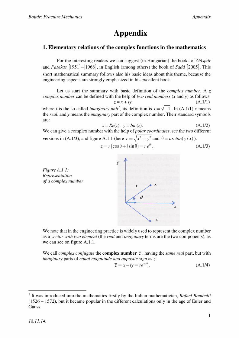
We can give a complex number with the help of polar coordinates, see the two different
versions in (A.1/3), and figure A.1.1 (here 2 2r x y= + and ( / )arctan y xθ = ):
( )cos sin iz r i r e θ= θ + θ = , (A.1/3)
Figure A.1.1: Representation of a complex number
We note that in the engineering practice is widely used to represent the complex number
as a vector with two element (the real and imaginary terms are the two components), as
we can see on figure A.1.1.
We call complex conjugate the complex number z , having the same real part, but with
imaginary parts of equal magnitude and opposite sign as z:
iz x iy re− θ= − = . (A.1/4)
1 It was introduced into the mathematics firstly by the Italian mathematician, Rafael Bombelli (1526 – 1572), but it became popular in the different calculations only in the age of Euler and
Gauss.
x
y
z
z
θ
r
Bojtár: Fracture Mechanics Appendix
2
18.11.14.
We shall use very often in the complex analysis the following differential operators:
where u (x, y) is the real and v (x, y) is the imaginary part of the complex function. For example:
2 2
2 2
2 2
( ) ( ) ( )
(2 )
( , ) , ( , ) 2 .
f z az bz a x iy b x iy
ax ay bx i axy by
u x y ax ay bx v x y axy by
= + = + + + =
= − + + + ⇒
= − + = +
Similarly to a complex number a complex function has also a conjugate pair:
( ) ( , ) ( , ).f z u x y iv x y= − (A.1/7)
The differentiation of the complex functions is also very important in the engineering
practice. Assuming the continuity of the functions we can define the differentiation at a
point 0z in a given domain D as follows:
0 00 0
( ) ( )( ) lim z
f z z f zf z
z∆ →
+ ∆ − ′ = ∆. (A.1/8)
If a complex function f(z) is differentiable in every points of the domain D, we call it
analytic (or holomorphic) function. Those points, where a function is not analytic we
shall call singular points.
Let us apply now the differential operators (A.1/5) for the function f (z):
1 1
( ) ( )2 2
u v v uf z u iv i
z x y x y
∂ ∂ ∂ ∂ ∂ ′ = + = + + − ∂ ∂ ∂ ∂ ∂ . (A.1/9)
Because the value of derivative defined by (A.1/8) will not depend from the path, where
the value of z∆ tends to zero, so the relationship (A.1/9) must give the same result in
both cases either 0 or 0x y∆ = ∆ = . According to this statement we can write (A.1/9)
as follows:
1 1 1 1
( )2 2 2 2
u v v uf z i i
x x y y
∂ ∂ ∂ ∂ ′ = + = + − ∂ ∂ ∂ ∂ . (A.1/10)
From comparison of the real and imaginary parts we obtain the so called Cauchy-Riemann equalities:
, .u v u v
x y y x
∂ ∂ ∂ ∂= = −
∂ ∂ ∂ ∂ (A.1/11)
If we use polar coordinates then (A.1/11) has the following form:
1 1
, .u v u v
r r r r
∂ ∂ ∂ ∂= = −
∂ ∂θ ∂θ ∂ (A.1/12)
From further differentiations of (A.1/11) we can proof that both u and v are harmonic
functions:
Bojtár: Fracture Mechanics Appendix
3
18.11.14.
0, 0u v∆ = ∆ = . (A.1/13)
There is also an important comment, that using (A.1/11) we can write the total differentiation of u with the help of the function v:
d d d d du u v v
u x y x yx y y x
∂ ∂ ∂ ∂= + = −
∂ ∂ ∂ ∂, (A.1/14)
namely if we know v, from (A.1/14) we can determine u. This is right of course in
opposite order, from u we can calculate the function v. Based on this nature u and v are
called conjugate functions.
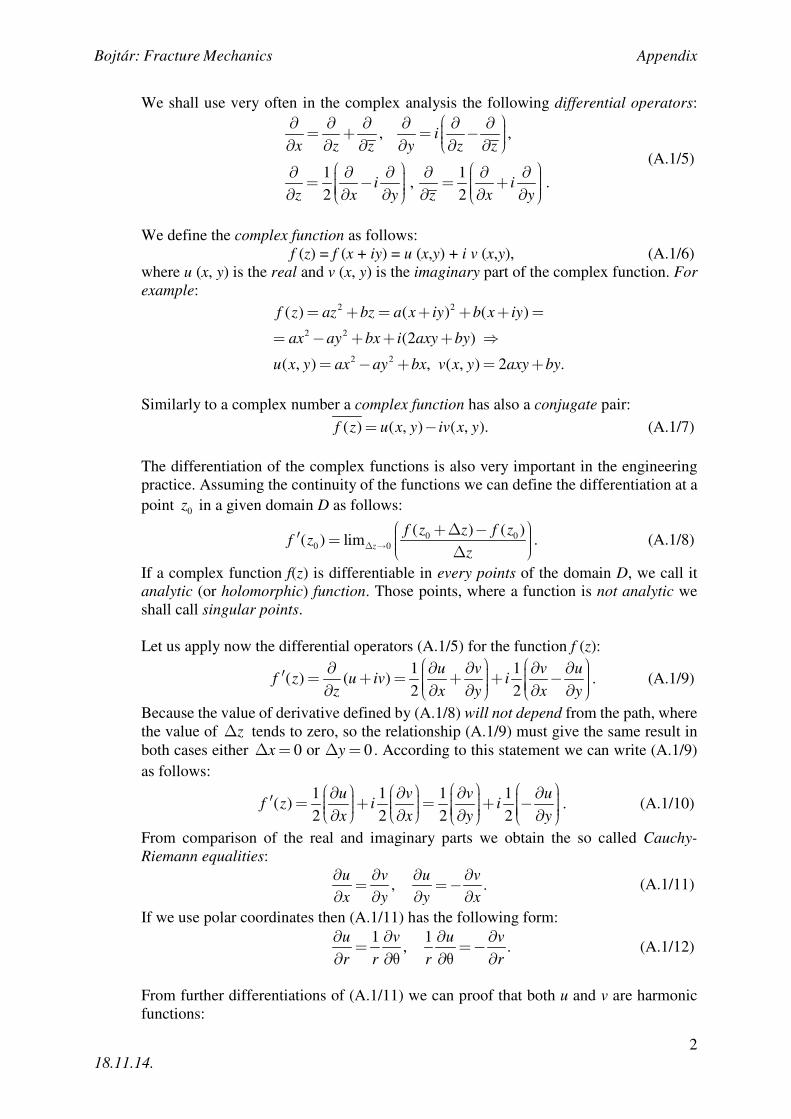
Let us discuss now the most important integral calculation rules on a complex
domain, using figure A.1.2:
Figure A.1.2: Path of integral calculation in a complex domain
Let us write along the curve C the line integral between the points 1 2andz z
( )( ) ( ) ( )( )( )d d d d d d d
C C C
f z z u iv x i y u x v y i u y v x= + + = − + +∫ ∫ ∫ . (A.1/15)
With the help of the Cauchy-Riemann equalities we can proof that the function is
analytic in every points of the domain D containig the curve C, then the value of the line
integral is independent from the path between the points 1 2andz z . From this statement
we can generate two important rules of complex functions:
- If the function f(z) is analytic inside – and in all points of – a closed curve C, then
( ) d 0
C
f z z =∫ . (A.1/16/a)
This is the so called Cauchy integral theorem.
- If the function f(z) is analytic inside – and in all points of – a closed curve C,
furthermore 0z is a point inside the curve, then 0( )f z can be calculated as follows:
0
0
1 ( )( ) d
2C
f zf z z
i z z=
π −∫ . (A.1/16/b)
This is the so called Cauchy integral formula.
We must often approximate a complex function with some kind of series. If f(z)
is analytic inside a closed curve C with the centre z = a, then we can approximate it –
inside the curve – with a Taylor series:
( )
)( ) ( ) ( ) ( ) ... ... ( ) ...
!
nnf a
f z f a f a z a z an
′= + − + + − + (A.1/17)
If a = 0 then (A.1/16) gives the Maclaurin series. From practical point of view it is an
interesting case when we have to make the series for the points lying between two
x
y
1z
2z
C
Bojtár: Fracture Mechanics Appendix
4
18.11.14.
concentric curves 1 2
andC C (we assume that 1 2
C C> ). In these cases we generate
Laurent series:
0 1
( ) ( )( )
n n
n nn n
Bf z A z a
z a
∞ ∞
= =
= − +−
∑ ∑ , (A.1/18/a)
where
1 2
1 1
0 0
1 ( ) 1 ( )d , 0,1, 2,..and d , 1, 2,...
2 ( ) 2 ( )n nn n
C C
f z f zA z n B z n
i z z i z z+ − += = = =
π − π −∫ ∫
(A.1/18/b)
If the analyzed domain contains singularities, the we must use different methods. We
discuss now only a specific type of the singularitis, this will be the so called „pole”
singularity. If f(z) is singular at the point z = a, but the product ( ) ( )nz a f z− is analytic
at any integer value of n, then the function f(z) has an n-order pole at the point z = a. In
this case we can approximate the product itself with a series at the point z = a:
0
1( ) ( ) ( ) , ( ) ( )
!
kn k n
k k kk
z a
dz a f z A z a A z a f z
k dz
∞
= =
− = − = −∑ . (A.1/19)
We obtain from this equation f(z) as follows:
0
( )( )
( )
k
k nk
z af z A
z a
∞
=
−=
−∑ . (A.1/20)
Let us integrate this relationship along a closed curve C, and the point a let be inside the
curve. Using the Cauchy integral formula we have:
1( )d 2 n
C
f z z i A −= π∫ . (A.1/21)
The terms 1n
A − are the “residuum” of the function f(z) at the pole z = a. If we know its
value, then we can determine the integral itself even in this singular case. Using the the
second term of the relationship (A.1/19):
1
1
1 d( )d 2 ( ) ( ) .
( 1)! d
nn
nC z a
f z z i z a f zn z
−
−
=
= π − −
∫ (A.1/22)
If we have more poles in one domain, then we determine the integral also with the help
of (A.1/22), but in this case we must summarize the residuum of all poles. This process
is called „residuum calculation method” in the complex calculus. If we apply this
technique together with the Cauchy integral formula, then we obtain the following
practical relations:
0, if 0,1 1
d1, if 0.2 ( )n
C
n
ni z
>ζ = =π ζ ζ − ∫ (A.1/23)
where C means now a circle with unit radius, and z lies inside the circle.
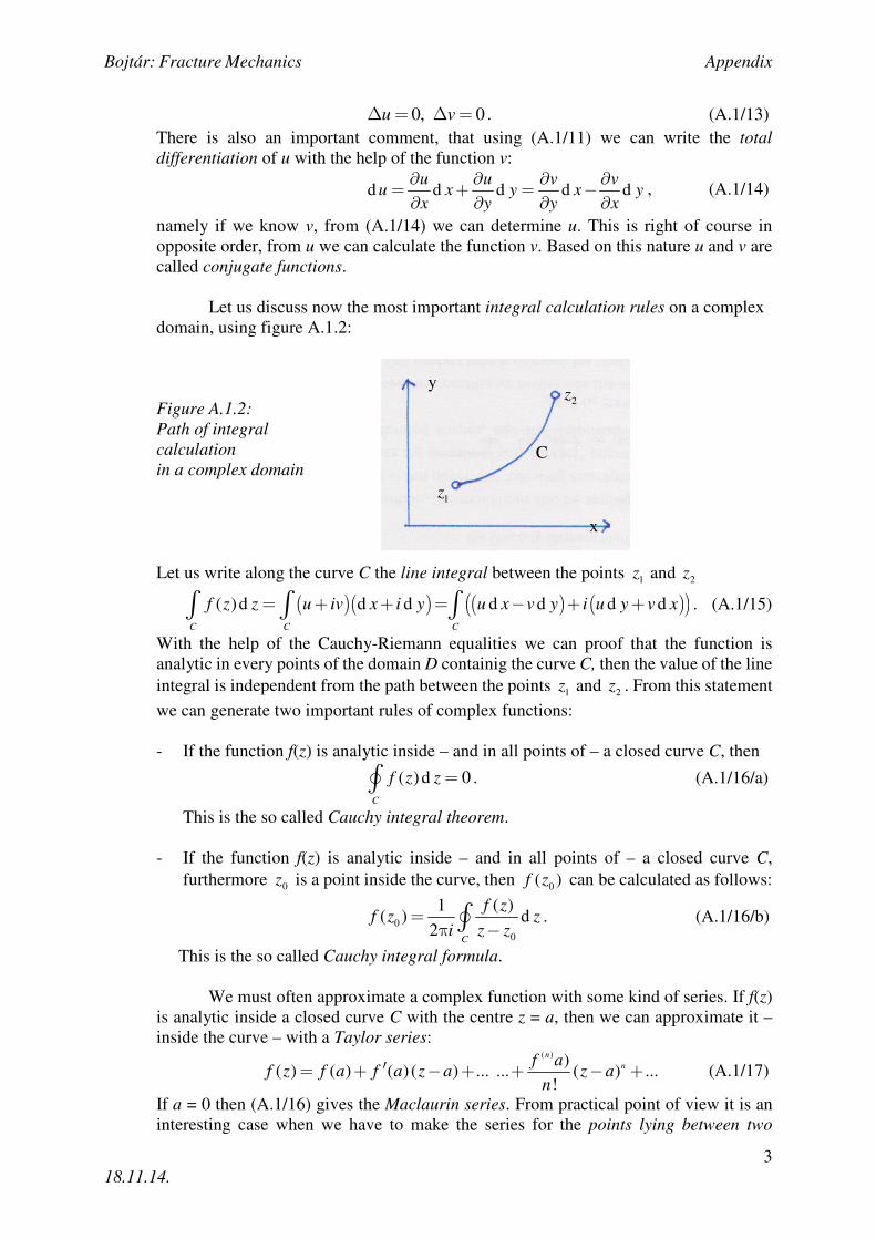
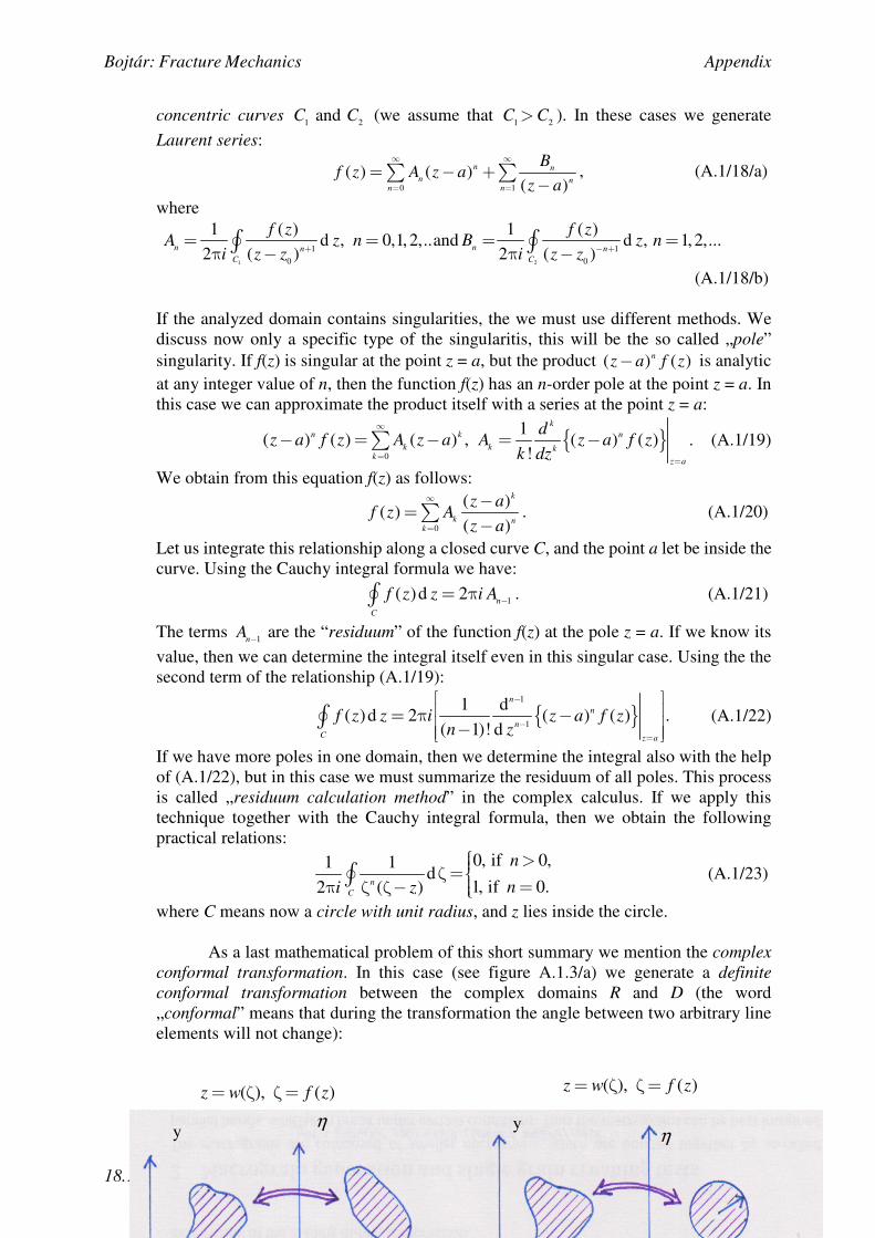
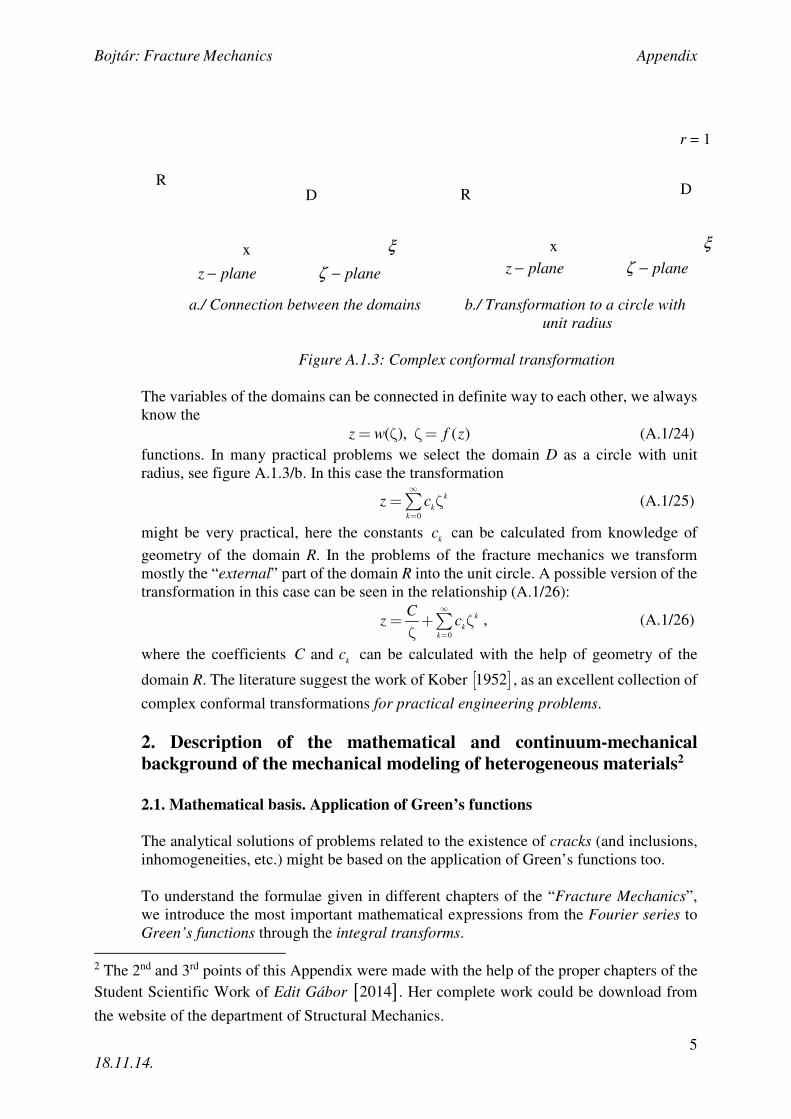
As a last mathematical problem of this short summary we mention the complex conformal transformation. In this case (see figure A.1.3/a) we generate a definite conformal transformation between the complex domains R and D (the word
„conformal” means that during the transformation the angle between two arbitrary line
elements will not change):
y
y η η
( ), ( )z w f z= ζ ζ = ( ), ( )z w f z= ζ ζ =
Bojtár: Fracture Mechanics Appendix
5
18.11.14.
a./ Connection between the domains b./ Transformation to a circle with unit radius
Figure A.1.3: Complex conformal transformation
The variables of the domains can be connected in definite way to each other, we always
know the
( ), ( )z w f z= ζ ζ = (A.1/24)
functions. In many practical problems we select the domain D as a circle with unit
radius, see figure A.1.3/b. In this case the transformation
0
k
kk
z c∞
=
= ζ∑ (A.1/25)
might be very practical, here the constants k
c can be calculated from knowledge of
geometry of the domain R. In the problems of the fracture mechanics we transform
mostly the “external” part of the domain R into the unit circle. A possible version of the
transformation in this case can be seen in the relationship (A.1/26):
0
k
kk
Cz c
∞
=
= + ζζ
∑ , (A.1/26)
where the coefficients andk
C c can be calculated with the help of geometry of the
domain R. The literature suggest the work of Kober [ ]1952 , as an excellent collection of
complex conformal transformations for practical engineering problems.
2. Description of the mathematical and continuum-mechanical background of the mechanical modeling of heterogeneous materials2 2.1. Mathematical basis. Application of Green’s functions
The analytical solutions of problems related to the existence of cracks (and inclusions,
inhomogeneities, etc.) might be based on the application of Green’s functions too.
To understand the formulae given in different chapters of the “Fracture Mechanics”,
we introduce the most important mathematical expressions from the Fourier series to
Green’s functions through the integral transforms.
2 The 2nd and 3rd points of this Appendix were made with the help of the proper chapters of the
Student Scientific Work of Edit Gábor [ ]2014 . Her complete work could be download from
the website of the department of Structural Mechanics.
x x ξ ξ
z plane planeζ− − z plane planeζ− −
R R D D
r = 1
Bojtár: Fracture Mechanics Appendix
6
18.11.14.
2.1.1. Fourier series and Fourier integrals
2.1.1.1. Fourier series
The Fourier series of a function ( )f x , where ( )f x is a continuous, integrable
function defined on the interval [ ],c c− :
0
1
( ) cos sin2
k kk
a k x k xf x a b
c c
π π∞
=
= + +
∑ . (A.2/1)
The coefficients ka and kb ( k : integer):
1( ) cos d , 0,1, 2,...
c
k
c
k xa f x x n
c c−
= =
∫
π, (A.2./2)
1( ) sin d , 1, 2,...
c
k
c
n xb f x x n
c c−
= =
∫
π, (A.2/3)
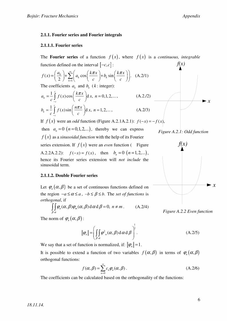
If ( )f x were an odd function (Figure A.2.1A.2.1): ( ) ( ),f x f x− = −
then ( )0 0,1,2,...na n= = , thereby we can express
( )f x as a sinusoidal function with the help of its Fourier
series extension. If ( )f x were an even function ( Figure
A.2.2A.2.2): ( ) ( )f x f x− = , then ( )0 1,2,...nb n= = ,
hence its Fourier series extension will not include the
sinusoidal term.
2.1.1.2. Double Fourier series
Let ( ),nϕ α β be a set of continuous functions defined on
the region a aα− ≤ ≤ , .b bβ− ≤ ≤ The set of functions is
orthogonal, if
( , ) ( , )d d 0, n m n m= ≠∫ ∫β α
ϕ α β ϕ α β α β . (A.2/4)
The norm of ( ),nϕ α β :
1
22 ( , )d dn n
= ∫ ∫β α
ϕ ϕ α β α β . (A.2/5)
We say that a set of function is normalized, if: 1nϕ = .
It is possible to extend a function of two variables ( ),f α β in terms of ( ),nϕ α β
orthogonal functions:
0
( , ) ( , )n nn
f cα β ϕ α β∞
=
=∑ . (A.2/6)
The coefficients can be calculated based on the orthogonality of the functions:
x
f(x)
Figure A.2.1: Odd function
x
f(x)
Figure A.2.2 Even function
Bojtár: Fracture Mechanics Appendix
7
18.11.14.
2
( , ) ( , )d d
( , )d d
n
n
n
f
c =∫ ∫
∫ ∫β α
β α
α β ϕ α β α β
ϕ α β α β. (A.2/7)
If the orthogonal set of functions are normalized, the denominator in (A.2/7) is 2 ( , ) d d 1n =∫ ∫
β α
ϕ α β α β , and the coefficients become:
( , ) ( , ) d dn nc f= ∫ ∫β α
α β ϕ α β α β . (A.2/8)
2.1.1.3. Double trigonometric series
Considering the orthogonal set of functions:
( ) ( ) ( ) ( )
( ) ( ) ( ) ( )
( ) ( ) ( ) ( ) ( )
1, cos , sin , cos , sin ,
cos cos , sin cos ,
cos sin , sin sin , ... , 1, 2,3,...
mx mx ny ny
mx ny mx ny
mx ny mx ny n m =
defined on the region xπ π− ≤ ≤ , yπ π− ≤ ≤ , it is leading to the system:
( ) ( ) ( )2
1, cos cos d dmn
y x
a f x y mx ny x yπ
= ∫ ∫ , (A.2/9)
( ) ( ) ( )2
1, sin cos d dmn
y x
b f x y mx ny x yπ
= ∫ ∫ , (A.2/10)
( ) ( ) ( )2
1, cos sin d dmn
y x
c f x y mx ny x yπ
= ∫ ∫ , (A.2.11)
( ) ( ) ( )2
1, sin sin d dmn
y x
d f x y mx ny x yπ
= ∫ ∫ , (A.2.12)
with , 1, 2,...m n = . Extending the possible values that ,m n can take by either 0m = or
0n = , the series expansion of function ( ),f x y can be written as:
, 0
( , ) ( cos( )cos( ) sin( ) cos( ) cos( )sin( )
sin( )sin( )) (A.2 /13)
mn mn mn mnm n
mn
f x y a mx ny b mx ny c mx ny
d mx ny
λ∞
=
= + + +
+
∑
with the coefficients
1for 0,
4
1for 0, 0 0, 0,
2
1 for , 0.
mn
m n
m n or m n
m n
λ
= =
= > = = > >
(A.2/14)
The [ ], , ,x y π π π π∈ − ×− variables and domain can be transformed into
[ ], , ,a a b bα β ∈ − ×− , where xa
πα= , y
b
πβ= .
2.1.1.4. Integral transforms
Bojtár: Fracture Mechanics Appendix
8
18.11.14.
The function ( )f x has a convergent integral3 on [ ]0,∞ if
0
( ) ( ) ( ) dfI f x K x x∞
= ∫α α (A.2/15)
is convergent. ( )fI α is the integral transform of function ( )f x by kernel4 ( )K xα .
If (A.2/15) is satisfied by only one particular ( )f x , then the integral (A.2/15) has an
inverse form:
0
( ) ( ) H( ) dff x I xα α α∞
= ∫ . (A.2/16)
If ( ) ( )K x H xα α= , then ( )K xα is a Fourier kernel, and the integral transform of
function ( )f x by a Fourier kernel ( )K xα is called the Fourier transform ( )F α of the
function:
( ) ( ) ( )0
dF f x K x xα α∞
= ∫ . (A.2/17)
The Mellin transform ( )K s of kernel ( )K x :
1
0
( ) ( ) dsK s K x x x∞
−= ∫ , (A.2/18)
where the kernel ( )K x itself is transformed by the Mellin kernel
( ) 1, sM x s x −= . (A.2/19)
If ( )K xα is a Fourier kernel, it has the property
3 An infinite series ( )0n
f n∞
=
∑ of non-negative terms ( )f x defined on the unbounded interval
[ ]0,∞ on which it is monotone decreasing, converges to a real number if and only if the
improper integral ( )0
df x x∞
∫ is finite. In this case, the improper integral is the limit of a definite
integral as the endpoint of the interval of integration approaches to infinity: ( )lim d
b
ba
f x x→∞ ∫ . If
the improper integral is finite, then the proof also gives the lower and upper bound for the
infinite series: ( ) ( ) ( ) ( )00 0
d 0 dn
f x x f n f f x x∞ ∞∞
=
≤ ≤ +∑∫ ∫ .
4 An integral transform is a particular type of mathematical operator, where the input is a
function ( )f x , the output is another function ( )fI α dependent on the choice of the kernel
function ( )K xα of variables x and α . There are some special integral transforms, such as
Fourier transform, the Mellin transform (http://en.wikipedia.org/wiki/Mellin_transform , see:
H. Mellin: "Über die fundamentelle Wichtigkeit des Satzes von Cauchy für die Theorie der Gamma- und hypergeometrischen Funktionen", Acta Soc. Sci. Fennica, 21:1 (1896) pp. 1–115),
and the identity transform (http://en.wikipedia.org/wiki/Identity_transform), they are
dependent only on the applied kernel function.
Bojtár: Fracture Mechanics Appendix
9
18.11.14.
( ) ( )1 1K s K s− = . (A.2/20)
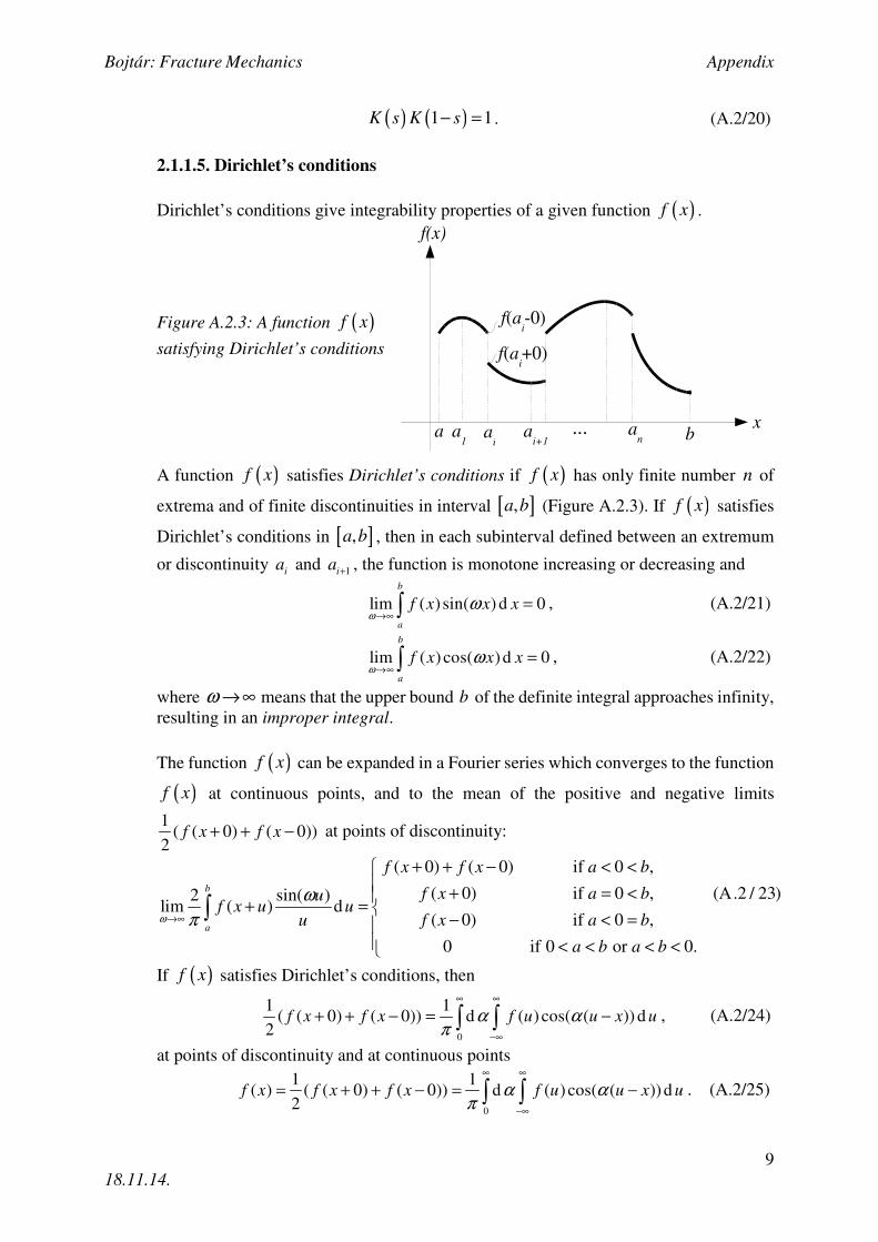
2.1.1.5. Dirichlet’s conditions
Dirichlet’s conditions give integrability properties of a given function ( )f x .
Figure A.2.3: A function ( )f x
satisfying Dirichlet’s conditions
A function ( )f x satisfies Dirichlet’s conditions if ( )f x has only finite number n of
extrema and of finite discontinuities in interval [ ],a b (Figure A.2.3). If ( )f x satisfies
Dirichlet’s conditions in [ ],a b , then in each subinterval defined between an extremum
or discontinuity ia and 1ia + , the function is monotone increasing or decreasing and
lim ( ) sin( ) d 0
b
a
f x x x→∞
=∫ωω , (A.2/21)
lim ( ) cos( ) d 0
b
a
f x x x→∞
=∫ωω , (A.2/22)
where ω →∞ means that the upper bound b of the definite integral approaches infinity,
resulting in an improper integral.
The function ( )f x can be expanded in a Fourier series which converges to the function
( )f x at continuous points, and to the mean of the positive and negative limits
1( ( 0) ( 0))
2f x f x+ + − at points of discontinuity:
( 0) ( 0) if 0 ,
( 0) if 0 , (A.2 / 23)2 sin( )lim ( ) d
( 0) if 0 ,
0 if 0 or 0.
b
a
f x f x a b
f x a buf x u u
f x a bu
a b a b
→∞
+ + − < < + = <
+ = − < =
< < < <
∫ω
ω
π
If ( )f x satisfies Dirichlet’s conditions, then
0
1 1( ( 0) ( 0)) d ( ) cos( ( )) d
2f x f x f u u x u
∞ ∞
−∞
+ + − = −∫ ∫α απ
, (A.2/24)
at points of discontinuity and at continuous points
0
1 1( ) ( ( 0) ( 0)) d ( ) cos( ( )) d
2f x f x f x f u u x u
∞ ∞
−∞
= + + − = −∫ ∫α απ
. (A.2/25)
x
f(x)
a bai
a1
an
...ai+1
f(ai-0)
f(ai+0)
Bojtár: Fracture Mechanics Appendix
10
18.11.14.
2.2.2.6. Integral theorems
If a function ( )f x has a convergent integral in interval [ ]0,∞ and satisfies Dirichlet’s
conditions, we can extend ( )f x in interval [ ],0−∞ such that ( ) ( )f x f x− = , i.e. by
constructing an even function. In this case, from (A.2/24) comes
0 0 0
2 2( ) cos( )d ( )cos( ) d ( ) cos( )dcf x x f F x
∞ ∞ ∞
= =∫ ∫ ∫α α η αη η α α απ π
, (A.2/26)
where the Fourier cosine transform of ( )f x is defined as
0
2( ) ( )cos( )dcF f
∞
= ∫α η αη ηπ
. (A.2.27)
If we extend ( )f x in the interval [ ],0−∞ such that ( ) ( )f x f x− = − , i.e. by constructing
an odd function, then, similarly to (A.2/26):
0 0 0
2 2( ) sin( )d ( )sin( ) d ( )sin( )dsf x x f F x
∞ ∞ ∞
= =∫ ∫ ∫α α η αη η α α απ π
, (A.2/28)
where the Fourier sine transform of ( )f x is
0
2( ) ( )sin( ) dsF f
∞
= ∫α η αη ηπ
. (A.2/29)
Noting that
( )( ) ( )( )0
cos d 2 cos d
m m
m
x xα η α α η α−
− = −∫ ∫ , (A.2/30)
( )( )sin d 0
m
m
xα η α−
− =∫ , (A.2/31)
from (A.2/25) it can be written that
( ) ( ) ( )( )
( ) ( )
0
1lim d cos d
1 1lim d d
2
m
m
mi x
mm
f x f x
f e α η
η η α η απ
η η απ
∞
→∞−∞
∞−
→∞−∞ −
= − =
= ⋅
∫ ∫
∫ ∫
(A.2/32)
which further implies
1( ) d ( ) d
2
i x if x e f e∞ ∞
−
−∞ −∞
= ∫ ∫α αηα η η
π. (A.2/33)
The Fourier integral of a function ( )f x is defined as
( )1
( ) d2
i xf x F e∞
−
−∞
= ∫αα α
π, (A.2/34/a)
where
1
( ) ( ) d2
i xF f x e x∞
−∞
= ∫αα
π. (A.2/34/b)
The Fourier integrals can be considered as limiting cases of the Fourier series, where
c → ∞ in (A.2/1).
Bojtár: Fracture Mechanics Appendix
11
18.11.14.
2.1.1.7. Convolution integrals
The convolution theorems can be used to evaluate integrals. The convolution of
functions ( )f x and ( )g x is defined as
( ) ( ) ( ) ( ) df g x f x g∞
−∞
∗ = −∫ η η η . (A.2/35)
Let us consider the Fourier transforms
1( ) ( ) d
2
itxF t f x e x∞
−∞
= ∫π, (A.2/36)
1( ) ( ) d
2
itxG t g x e x∞
−∞
= ∫π. (A.2/37)
The convolution of ( )f x and ( )g x can be written with the help of their Fourier
transforms ( )F t and ( )G t as
( )( ) ( ) ( ) d ( ) ( )ditxf g x F t G t e t f x g∞ ∞
−
−∞ −∞
∗ = = −∫ ∫ η η η . (A.2/38)
In a special case, when 0x = , the convolution ( )( )f g x∗ can be written as
( ) ( )0 ( ) ( ) d ( ) ( )df g F t G t t f g∞ ∞
−∞ −∞
∗ = = −∫ ∫ η η η . (A.2/39)
If ( )f x is an even function, i.e. ( ) ( )f x f x− = , then we can replace ( )F t with the
Fourier cosine transform ( )cF t and ( )G t with ( )cG t , respectively (see (A.2/27)).
Hence, (A.2/39) becomes
( )( )0 0
0 ( ) ( ) d ( ) ( ) dc cf g F t G t t f g∞ ∞
∗ = =∫ ∫ η η η . (A.2/40)
2.1.1.8. Fourier transforms of derivatives of a function
The formula for the Fourier transform of the r -th derivative of a function ( )f x can be
obtained by integrating by parts
( ) 1 d ( )( ) d
d2
rr i x
r
f xF e x
x
∞
−∞
= ∫αα
π. (A.2/41)
The general formula can be written as ( ) ( ) ( ) ( )r rF i Fα α α= − . (A.2/42)
Bojtár: Fracture Mechanics Appendix
12
18.11.14.
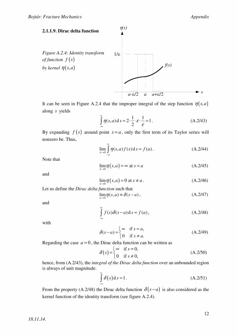
2.1.1.9. Dirac delta function
Figure A.2.4: Identity transform
of function ( )f s
by kernel ( ),s aη
It can be seen in Figure A.2.4 that the improper integral of the step function ( ),s aη
along s yields
1 1( , )d 2 1
2s a s
∞
−∞
= ⋅ ⋅ ⋅ =∫η εε
. (A.2/43)
By expanding ( )f s around point s a= , only the first term of its Taylor series will
nonzero be. Thus,
0lim ( , ) ( ) d ( )s a f s s f a
∞
→−∞
=∫εη . (A.2/44)
Note that
( )0
lim , at s a s aε
η→
= ∞ = (A.2/45)
and
( )0
lim , 0 at s a s aε
η→
= ≠ . (A.2/46)
Let us define the Dirac delta function such that
0lim ( , ) ( )s a s aε
η δ→
≡ − , (A.2/47)
and
( ) ( )d ( )f s s a s f a∞
−∞
− =∫ δ , (A.2/48)
with
if ,( )
0 if .
s as a
s aδ
∞ =− =
≠ (A.2/49)
Regarding the case 0a = , the Dirac delta function can be written as
( )if 0,
0 if 0,
ss
sδ
∞ ==
≠ (A.2/50)
hence, from (A.2/43), the integral of the Dirac delta function over an unbounded region
is always of unit magnitude:
( )d 1s sδ∞
−∞
=∫ . (A.2/51)
From the property (A.2/48) the Dirac delta function ( )s aδ − is also considered as the
kernel function of the identity transform (see figure A.2.4).
sa
f(s)
h(s)
1/e
a+e/2a-e/2
Bojtár: Fracture Mechanics Appendix
13
18.11.14.
2.1.2. Green’s function
2.1.2.1. General definition of Green’s function
In general, Green’s function ( ),G x s is the impulse response of an inhomogeneous
partial differential equation
( ) ( )Lu x f x= (A.2.52)
defined on a domain with prescribed boundary or initial conditions:
( ) 0Du x = . (A.2/53)
At time-invariant, linear problems, the impulse response ( ),G x s of a linear
transformation ( )L L x= acting at point x s= , is the image of the Dirac delta function
( )x sδ − under the transformation:
( ) ( ),LG x s x sδ= − , (A.2/54)
where the case x s≠ results in a homogeneous equation due to the property of Dirac’s
delta function given in (A.2/49). If the kernel of L is non-trivial, then the Green’s
function of the problem is not unique. In general, due to the prescribed boundary or
initial conditions, Green’s function is always unique.
The convolution of Green’s function ( ),G x s with any arbitrary function ( )f s on that
domain is the solution for the inhomogeneous differential equation for ( )f s :
( ) ( ) ( ) ( ) ( ), d dLG x s f s s x s f s s f x= − =∫ ∫δ , (A.2/55)
where the Dirac delta function appeared as a kernel function of the identity transform
(see (A.2/48)). Substituting (A.2/52 into (A.2/55) we have
( ) ( ) ( ), dLu x LG x s f s s= ∫ . (A.2/56)
Since the linear operator L is only a function of x , it can be taken out from the
integration along s and
( ) ( ) ( ), dLu x L G x s f s s= ∫ , (A.2/57)
which implies
( ) ( ) ( ), du x G x s f s s= ∫ . (A.2/58)
It is the exact solution of the inhomogeneous partial differential equation (A.2/52). The
difficult part of finding the solution with the help of Green’s function is finding the Green’s function itself for a given linear operator L . Moreover, the evaluation of the
integration in (A.2/57) is quite complicated, but this method gives a theoretically exact
result for inhomogeneous partial differential equations.
2.1.2.2. Mechanical interpretation of Green’s function
In applied mechanics, Green’s functions are used to solve inhomogeneous boundary value problems, such as the general boundary value problem of mechanics defined in
the following, where body forces appearing in the elastic media are also considered. In
anisotropic elastic media, the equilibrium equations (Cauchy equations):
, 0i j j ibσ + = , (A.2/59)
where ib is the vector of body force per unit volume.
Bojtár: Fracture Mechanics Appendix
14
18.11.14.
The constitutive equations:
,i j i j k l kl i j k l k lC C uσ ε= = , (A.2/60)
where k lε denotes the small elastic strains and i j k lC stands for the elastic stiffness tensor
of the media. Substituting the stresses in (A.2/60) into the equilibrium equation (F.2/59),
we obtain:
,i j k l k l j iC u b= − . (A.2/61)
If ib is concentrated, acts at point 'x x= in
direction mx , and its magnitude is unity, then
0 if ,
( ') if ,i
i mb
x x i mδ
≠=
− = (A.2/62)
or it can be written as:
( )( ') 1,2,3i imb x x iδ δ= − = , (A.2/63)
where ( )'x xδ − is the Dirac delta function and
i jδ indicates the Kronecker delta tensor:
1 if ,
0 if .ij
i j
i jδ
==
≠ (A.2./64)
Based on (A.2/63), equation (A.2/61) can be
rewritten in a form
( ),
( ')m
i j k l k l j imC u x xδ δ= − − , (A.2/65)
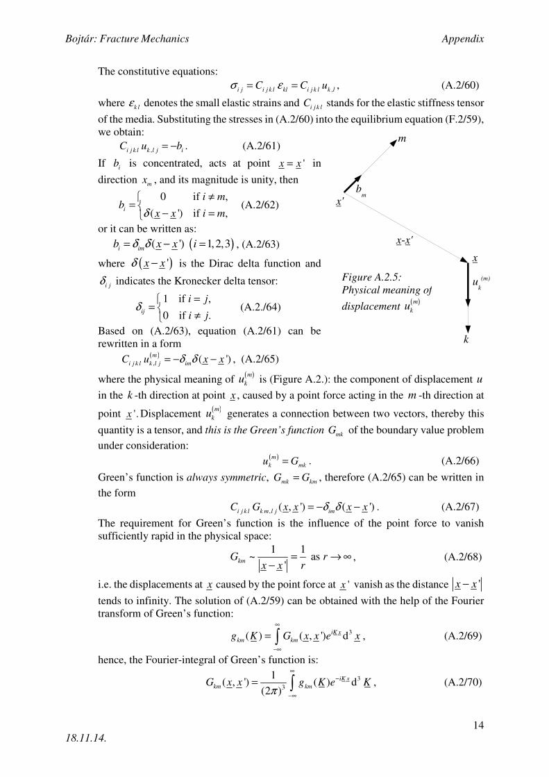
where the physical meaning of ( )m
ku is (Figure A.2.): the component of displacement u
in the k -th direction at point x , caused by a point force acting in the m -th direction at
point '.x Displacement ( )m
ku generates a connection between two vectors, thereby this
quantity is a tensor, and this is the Green’s function mkG of the boundary value problem
under consideration: ( )m
k mku G= . (A.2/66)
Green’s function is always symmetric, mk kmG G= , therefore (A.2/65) can be written in
the form
,( , ') ( ')i j k l k m l j imC G x x x xδ δ= − − . (A.2/67)
The requirement for Green’s function is the influence of the point force to vanish
sufficiently rapid in the physical space:
1 1~ as
'kmG r
x x r= → ∞
−, (A.2/68)
i.e. the displacements at x caused by the point force at 'x vanish as the distance 'x x−
tends to infinity. The solution of (A.2/59) can be obtained with the help of the Fourier
transform of Green’s function:
3( ) ( , ') diK xkm kmg K G x x e x
∞
−∞
= ∫ , (A.2/69)
hence, the Fourier-integral of Green’s function is:
3
3
1( , ') ( ) d
(2 )
iK xkm kmG x x g K e K
∞−
−∞
= ∫π, (A.2/70)
x'
x
x-x'
m
bm
k
uk
(m)Figure A.2.5: Physical meaning of
displacement ( )m
ku
Bojtár: Fracture Mechanics Appendix
15
18.11.14.
where K is the Fourier vector in Fourier space. Multiplying (A.2/67) by ( )'iK x xe − and
integrating over the unbounded domain, we have
( ) ( )' '3 3
, ( , ') d ( ') diK x x iK x x
i j k l km l j imC G x x e x x x e xδ δ∞ ∞
− −
−∞ −∞
= − −∫ ∫ , (A.2/71)
where ( )3 3d d 'x x x= − because of the fixed position of 'x . Taking into account
(A.2/68), integration by parts yield
( ) ( )3, ' d 'j l i j k l km imK K C G x x x x δ∞
−∞
− − = −∫ . (A.2/72)
If we define a unit vector T along vector 'x x− , we can express Green’s function as
( ) ( )( )
( )sgn
, 'km km km
sG x x G sT G T
s= = , (A.2/73)
and the nα -th derivative of Green’s function:
1 2 1 2 1 2, ... , ... , ...
sgn( )( , ') ( ) ( )
n n nkm km kmn
sG x x G sT G T
sα α α α α α α α α= = , (A.2/74)
where s is an algebraically signed scalar expressing the distance between x and 'x .
2.1.2.3. Isotropic Green’s function
In case of isotropic elastic media, we can define the elastic stiffness tensor i j k lC with
the help of the Kronecker delta tensor i jδ and Lamé’s constants λ and µ :
( )i j k l ij kl ik jl il jkC λδ δ µ δ δ δ δ= + + . (A.2/75)
The isotropic Green’s function can be expressed by
2
21( ') '
8 2km km
k m
G x x x xx x
λ µδ
πµ λ µ
+ ∂− = ∇ − −
+ ∂ ∂ (A.2/76)
with
2 2'
'x x
x x∇ − =
−. (A.2/77)
The displacement ( )m
ku is independent of the positions x and 'x , it is only the function
of the distance 'x x− between them, resulting in Green’s function being translation
invariant. At linear, time-invariant problems, Green’s function is always translation-
invariant, and due to this property, it acts as a convolution operator:
( ) ( ), ' 'G x x G x x= − . (A.2/78)
2.2. Mechanical basis. Definitions of eigenstrains and eigenstresses, basic equations
2.2.1. General theory of eigenstrains
2.2.1.1. Definition of eigenstrains
Eigenstrains are such nonelastic strains as thermal expansion, phase transformation,
initial strains, plastic strains or misfit strains. This type of strain appears in a body even
if there is no external load acting on it.
Bojtár: Fracture Mechanics Appendix
16
18.11.14.
Eigenstresses are such self-equilibrated internal stresses caused by eigenstrains in
bodies which are free from any other external force and surface constraints. This stress
field is created by the incompatibility of the eigenstrains.
2.2.1.1. Fundamental equations of elasticity
If a free body D is subjected to a given distribution of eigenstrains, otherwise it is free
from any external surface or body force, then the actual strain ( i jε ) can be computed
as the sum of the eigenstrains ( ijε ∗) and the elastic strains ( i je ) defined by Hooke’s law
in elastic bodies:
i j i j i jeε ε ∗= + . (A.2/79)
The compatibility equation written for the total strain:
, ,
1( )
2i j i j j iu uε = + . (A.2/80)
The connection between the elastic strains and stresses:
( )i j i j k l kl i j k l kl klC e Cσ ε ε ∗= = − , (A.2/81)
and its inverse form:
1
i j i j i j k l k lCε ε σ∗ −− = , (A.2/82)
which − for isotropic materials − can be expressed with the help of Lamé’s constant
(also known as shear modulus) µ and Poisson’s ratio ν :
1
2 1
i j k k
i j i j i j
δ σ νε ε σ
µ ν∗
− = − +
. (A.2/83)
If body D is not free from external forces, then the actual stress field is the sum of the
eigenstress of the free body and the solution of the boundary value problem. The
equations of equilibrium if we neglect the body forces:
,
0, 1,2,3i j j iσ = = . (A.2/84)
The boundary conditions for free external surface forces:
0i j jnσ = , (A.2/85)
where in is the outward unit normal vector on the surface of D .
We can express the stress field with the help of eigenstrains and the displacement field
based on (A.2/80) and (A.2/81):
,( )i j i j k l k l k lC uσ ε ∗= − . (A.2/86)
The conditions (A.2/84) and (A.2/85) yield:
, ,i j k l k l j i j k l k l jC u C ε ∗= , (A.2/87)
,i j k l k l j i j k l k l jC u n C nε ∗= . (A.2/88)
From (A.2/87) we can see that the eigenstrain contributes as a body force ib :
,i j k l k l j iC u b= − . (A.2/89)
Bojtár: Fracture Mechanics Appendix
17
18.11.14.
It is also visible that in (A.2/88) the eigenstrain behaves like a surface force on the
boundary of D . Summarizing these two observations, the elastic displacement field in
an elastic body caused by a given eigenstrain i jε ∗ is equivalent to that caused by a body
force ,i j k l k l jC ε ∗− and surface force i j k l k l jC nε ∗. In most cases, D
is considered as an infinitely extended body, thus (A.2/85) can be
replaced with the following condition:
(x) 0 as ij xσ → → ∞ . (A.2/90)
The compatibility conditions can be given with the help of the
third-order Levi-Civita permutation tensor :pkiε
,
0p k i q l j i j k l =ε ε ε . (A.2/91)
The fundamental equations to be
solved are equations (A.2/87).
Several methods for calculating the
associated elastic fields under a given distribution of eigenstrains were developed. The
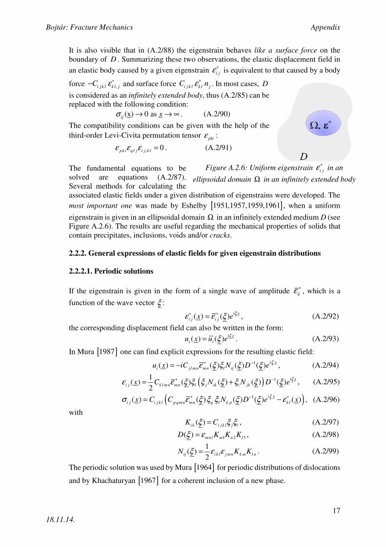
most important one was made by Eshelby [ ]1951,1957,1959,1961 , when a uniform
eigenstrain is given in an ellipsoidal domain Ω in an infinitely extended medium D (see
Figure A.2.6). The results are useful regarding the mechanical properties of solids that
2.2.2. General expressions of elastic fields for given eigenstrain distributions
2.2.2.1. Periodic solutions
If the eigenstrain is given in the form of a single wave of amplitude ijε ∗, which is a
function of the wave vector ξ :
( ) ( )i x
i j i jx eξε ε ξ∗ ∗= , (A.2/92)
the corresponding displacement field can also be written in the form:
( ) ( )i x
i iu x u eξξ= . (A.2/93)
In Mura [ ]1987 one can find explicit expressions for the resulting elastic field:
1( ) ( ) ( ) ( )i x
i j l mn mn l iju x iC N D eξε ξ ξ ξ ξ∗ −= − , (A.2/94)
( ) 11( ) ( ) ( ) ( ) ( )
2
i x
i j k l m n m n l j ik i jkx C N N D eξ
ε ε ξ ξ ξ ξ ξ ξ ξ∗ −= + , (A.2/95)
( )1( ) ( ) ( ) ( ) ( )i x
i j i j k l p qmn mn q l k p k lx C C N D e xξ
σ ε ξ ξ ξ ξ ξ ε∗ − ∗= − , (A.2/96)
with
( )i k i j k l j lK Cξ ξ ξ= , (A.2/97)
1 2 3
( ) mnl m n lD K K Kξ ε= , (A.2/98)
1
( )2
ij i k l j m n k m l nN K Kξ ε ε= . (A.2/99)
The periodic solution was used by Mura [ ]1964 for periodic distributions of dislocations
and by Khachaturyan [ ]1967 for a coherent inclusion of a new phase.
Figure A.2.6: Uniform eigenstrain i j∗ε in an
ellipsoidal domain Ω in an infinitely extended body D
Bojtár: Fracture Mechanics Appendix
18
18.11.14.
2.2.2.2. Method of Fourier series and Fourier integrals
If the eigenstrain is given in the Fourier series form:
( ) ( )i x
i j i jx e∗ ∗=∑ ξε ε ξ , (A.2/100)
its solution is the superposition of the elastic fields of single waves of the form (A.2/92):
1( ) ( ) ( ) ( )i x
i j l m n mn l i ju x i C N D e∗ −= − ∑ ξε ξ ξ ξ ξ , (A.2/101)
( ) 11( ) ( ) ( ) ( ) ( )
2
i x
i j k l m n m n l j i k i j kx C N N D e−= +∑ ξε ε ξ ξ ξ ξ ξ ξ ξ , (A.2/102)
( )1( ) ( ) ( ) ( ) ( )i x
i j i j k l p qmn mn q l k p k lx C C N D e x∗ − ∗= −∑ ξσ ε ξ ξ ξ ξ ξ ε . (A.2/103)
If i j∗ε is given in the Fourier integral form:
( ) ( ) di x
i j i jx e∞
∗ ∗
−∞
= ∫ξε ε ξ ξ , (A.2/104)
where
3( ) (2 ) ( ) d
i x
i j i j x e x∞
−∗ − ∗
−∞
= ∫ξε ξ π ε , (A.2/105)
the corresponding displacement, strain and stress field:
1( ) ( ) ( ) ( ) di x
i j l mn mn l i ju x i C N D e∞
∗ −
−∞
= − ∫ξε ξ ξ ξ ξ ξ , (A.2/106)
( ) 11( ) ( ) ( ) ( ) ( ) d
2
i x
i j k l mn mn l j ik i jkx C N N D e∞
∗ −
−∞
= +∫ξε ε ξ ξ ξ ξ ξ ξ ξ ξ , (A.2/107)
1( ) ( ) ( ) ( ) d ( )i x
i j i j k l p q mn mn q l k p k lx C C N D e x∞
∗ − ∗
−∞
= −
∫
ξσ ε ξ ξ ξ ξ ξ ξ ε . (A.2/108)
2.2.2.3. Method of Green’s functions
The integral representations of the elastic field can also be given with the help of Green’s
functions, it is called the fundamental solution. If Green’s function5 ( ), 'i jG x x is
defined as:
( ')3 1( ') (2 ) ( ) ( ) d
i x x
i j i jG x x N D e∞
−− −
−∞
− = ∫ξπ ξ ξ ξ , (A.2/109)
the solution:
,( ) ( ') ( ') d 'i j l mn mn i j lu x C x G x x x∞
∗
−∞
= − −∫ ε , (A.2.110)
, ,
1( ) ( ')( ( ') ( ')) d '
2i j k l mn mn ik l j j k l ix C x G x x G x x x
∞∗
−∞
= − − + −∫ε ε , (A.2/111)
,( ) ( ') ( ') d ' ( )i j i j k l p q m n mn k p ql k lx C C x G x x x x∞
∗ ∗
−∞
= − − +
∫σ ε ε . (A.2/113)
5 Having the property of translation invariance, Green’s function ( ), 'i jG x x is only a function
of the distance between ix and 'ix , thus it can be written as ( )'ijG x x− .
Bojtár: Fracture Mechanics Appendix
19
18.11.14.
Explicit expressions for Green’s functions are only available for isotropic and transversely isotropic materials, otherwise the Fourier integral forms are more
convenient.
2.2.3. Static Green’s functions
The equations of equilibrium with respect to a displacement ( )'k mG x x− when the body
force ( )'im x xδ δ − is applied:
,
( ') ( ') 0i j k l k m l j i mC G x x x x− + − =δ δ . (A.2/114)
2.2.3.1. Isotropic materials
For isotropic materials, Lord Kelvin found the Green’s function, expressing it with the
help of Lamé’s constants λ , µ and/or Poisson’s ratio ν :
2
3
4
2
( 2 ) ( )( ) (2 ) d
( 2 )
1(3 4 )
16 (1 )
i xij i j
i j
i j
ij
G x e
x x
x x
∞−
−∞
+ − += =
+
= − +
−
∫ξλ µ δ ξ λ µ ξ ξ
π ξµ λ µ ξ
ν δπµ ν
, (A.2/114)
where 'ix is taken as zero without the loss of generality, and
1
2( )i ix x x= .
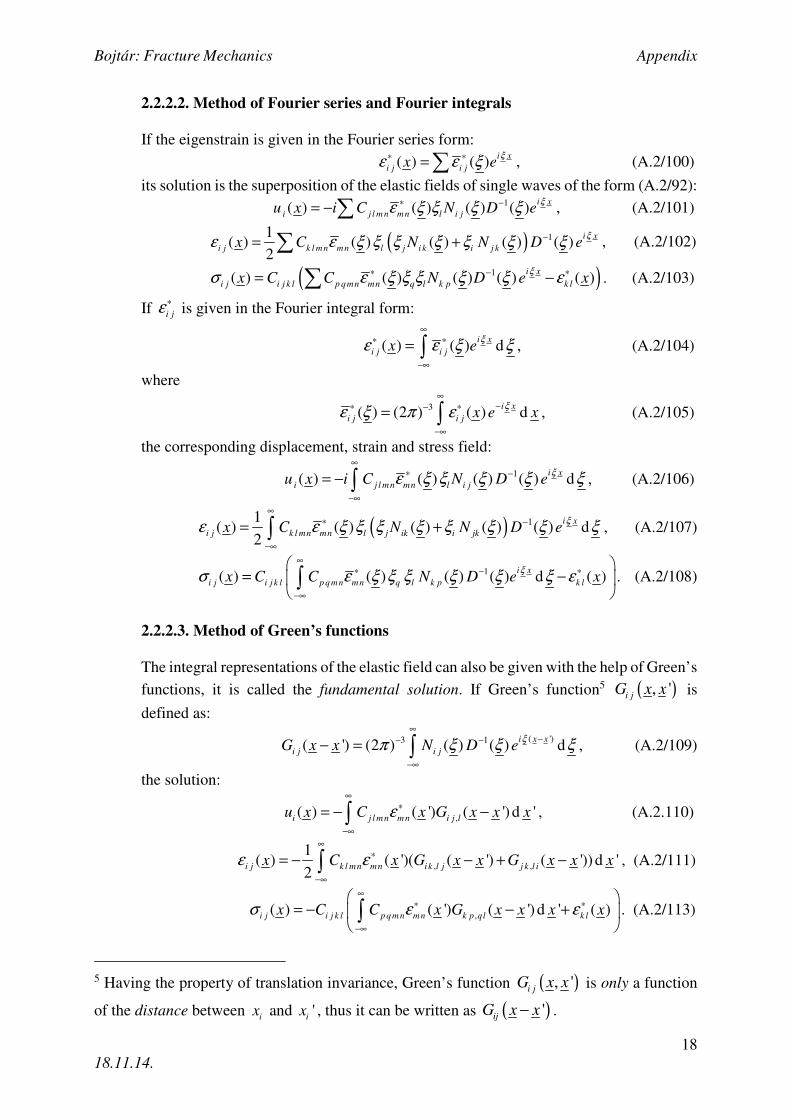
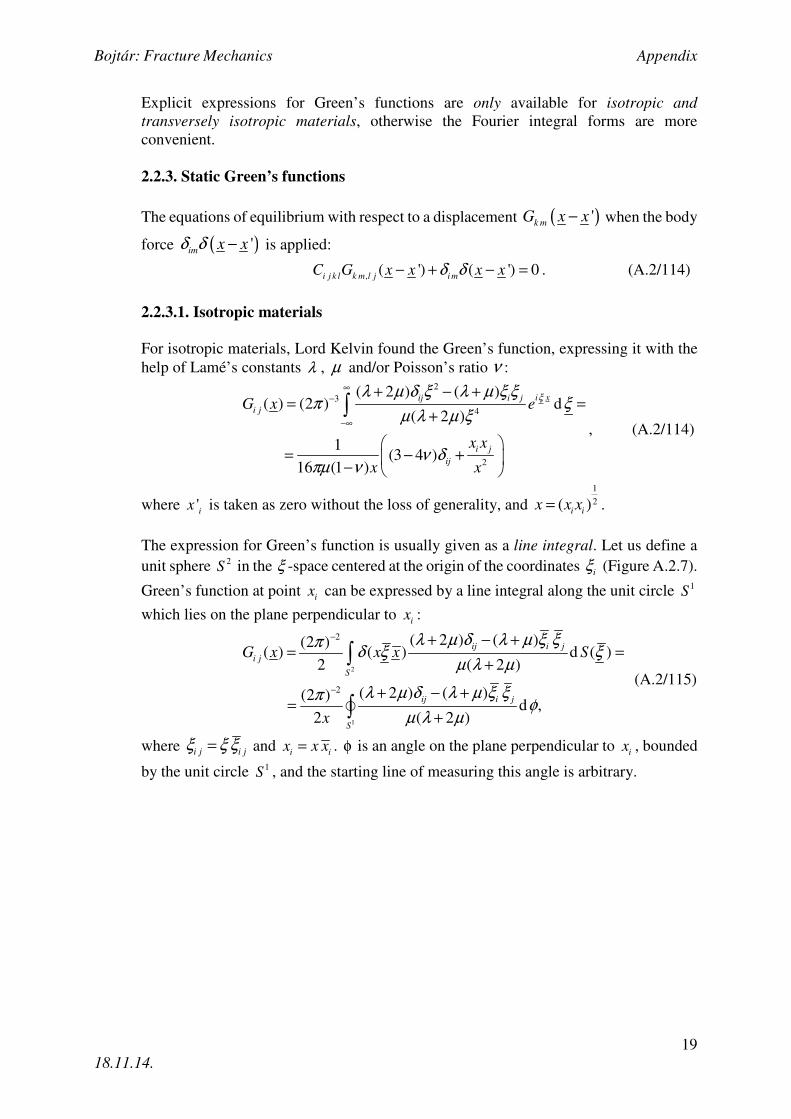
The expression for Green’s function is usually given as a line integral. Let us define a
unit sphere 2S in the ξ -space centered at the origin of the coordinates iξ (Figure A.2.7).
Green’s function at point ix can be expressed by a line integral along the unit circle 1S
which lies on the plane perpendicular to ix :
2
1
2
2
( 2 ) ( )(2 )( ) ( ) d ( )
2 ( 2 )
( 2 ) ( )(2 )d ,
2 ( 2 )
ij i j
i j
S
ij i j
S
G x x x S
x
−
−
+ − += =
+
+ − +=
+
∫
∫
λ µ δ λ µ ξ ξπδ ξ ξ
µ λ µ
λ µ δ λ µ ξ ξπφ
µ λ µ
(A.2/115)
where i j i j=ξ ξ ξ and i ix x x= . φ is an angle on the plane perpendicular to ix , bounded
by the unit circle 1S , and the starting line of measuring this angle is arbitrary.
Bojtár: Fracture Mechanics Appendix
20
18.11.14.
Figure A.2.7: Unit sphere 2S and unit circle 1S in ξ -space
2.2.3.2. Anisotropic materials
For anisotropic materials, the surface- and line integral expression of Green’s functions
are the following:
2 1
1 1
2 2
1 1( ) ( ) ( ) ( )d ( ) ( ) ( )d
8 8i j i j i j
S S
G x x x N D S N Dx
− −= =∫ ∫δ ξ ξ ξ ξ ξ ξ φπ π
. (A.2/116)
2.2.3.3. Kröner’s formula
Since ( ) ( )1
i jN D−ξ ξ is a continuous function on 2S , it can be extended into a series of
surface harmonic functions, which is any linear combination of spherical harmonics (set
of solution of Laplace’s equation):
1
0
( ) ( ) ( )ij nn
N D Uξ ξ ξ∞
−
=
=∑ , (A.2/117)
where
2
12 1( ) ( ') ( ') ( ')d ( '), 0,1,2,...
4n n ij
S
nU P N D S n−+
= =∫ξ ξξ ξ ξ ξπ
(A.2/118)
and nP is the Legendre polynomial6. The solution of Legendre’s differential equation
for 0,1, 2,...n = form a polynomial sequence of orthogonal polynomials called the
Legendre polynomials. Each ( )nP z polynomial is an n -th degree polynomial:
Kröner’s formula is a series expression of Green’s function for general anisotropic
materials using surface harmonic functions:
0
1( ) (0) ( )
4i j n n
n
G x P U xx
∞
=
= ∑π
. (A.2.120)
Kröner’s formula was modified by Mura and Kinoshita [ ]1971 , their solution is
continuously differentiable:
2
1
2
1( ) ( ) ( ) d ( )
16i j i j
S
G x N D x S−= ∆ ∫ ξ ξ ξ ξπ
. (A.2/121)
2.2.3.4. Derivatives of Green’s functions
We note that in the solution of eigenstrain problems we usually need the derivatives of
Green’s function. The formulae can be found in the previous section in (A.2/74),
furthermore in Mura [ ]1987 found by Barnett [ ]1972 and Willis [ ]1975 .
3. Mechanical study on the environment of inclusions. Analytical solutions for determination of the resulting elastic field 3.1. Inclusions
3.1.1. Definition of inclusion
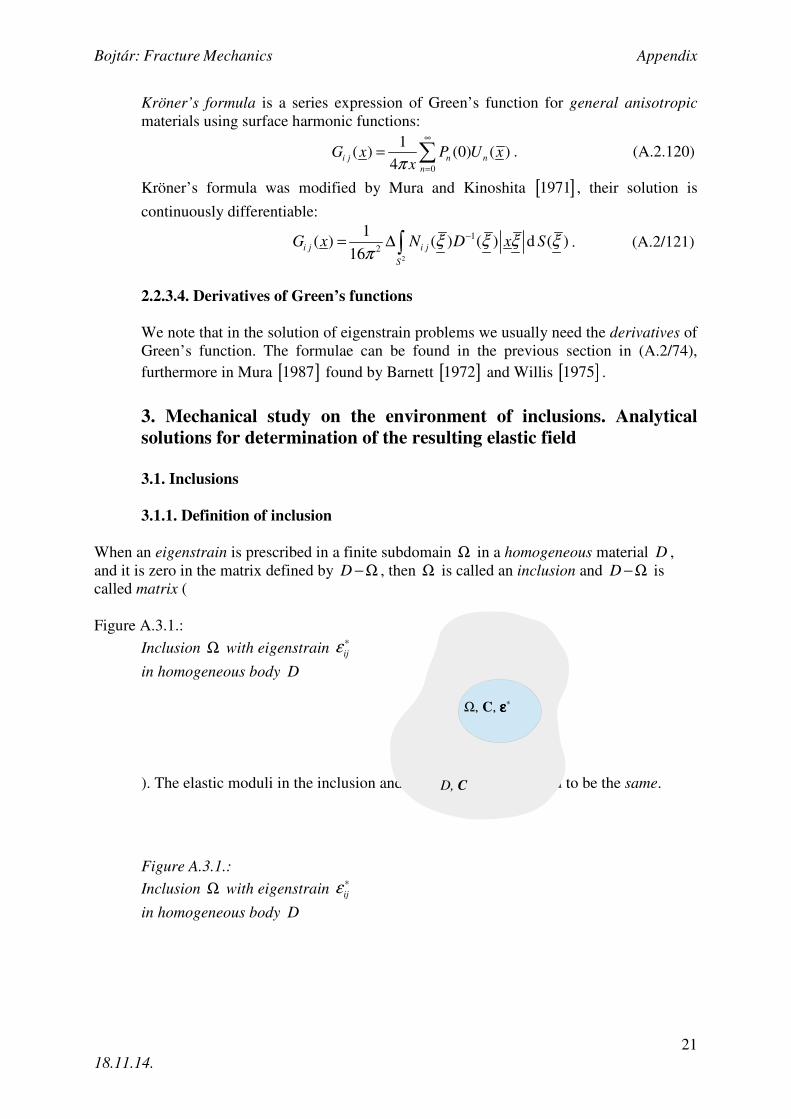
When an eigenstrain is prescribed in a finite subdomain Ω in a homogeneous material D ,
and it is zero in the matrix defined by D −Ω , then Ω is called an inclusion and D −Ω is
called matrix (
Figure A.3.1.:
Inclusion Ω with eigenstrain ijε ∗
in homogeneous body D
). The elastic moduli in the inclusion and in the matrix is assumed to be the same.
Figure A.3.1.:
Inclusion Ω with eigenstrain ijε ∗
in homogeneous body D
D, C
Ω, C, εεεε∗
Bojtár: Fracture Mechanics Appendix
22
18.11.14.
The elastic field due to the inclusion can be written with the help of Green’s functions:
,( ) ( ') ( ') d 'i j l mn mn i j lu x C x G x x x∗
Ω
= − −∫ ε , (A.3/1)
, ,
1( ) ( ')( ( ') ( '))d '
2i j k l mn mn i k l j j k l ix C x G x x G x x x∗
Ω
= − − + −∫ε ε , (A.3/2)
,( ) ( ') ( ') d ' ( )i j i j k l p q mn m n k p ql k lx C C x G x x x x∗ ∗
Ω
= − − +
∫σ ε ε , (A.3/3)
or, considering its Fourier integral forms:
( ')3 1( ) (2 ) ( ') ( ) ( ) d d 'i x x
i j l mn mn l iju x i C x N D e x∞
−− ∗ −
−∞ Ω
= − ∫ ∫ξπ ε ξ ξ ξ ξ , (A.3/4)
( ) ( ')3 1
( )
1(2 ) ( ') ( ) ( ) ( ) d d '
2
i j
i x x
k l mn mn l j i k i j k
x
C x N N D e x∞
−− ∗ −
−∞ Ω
=
= +∫ ∫ξ
ε
π ε ξ ξ ξ ξ ξ ξ ξ, (A.3/5)
( ')3 1
( )
(2 ) ( ') ( ) ( ) d d ' ( )
i j
i x x
i j k l p qmn mn q l k p k l
x
C C x N D e x x∞
−− ∗ − ∗
−∞ Ω
=
= −
∫ ∫
ξ
σ
π ε ξ ξ ξ ξ ξ ε,(A.3/6)
where ( ) 0k l xε ∗ = for x D∈ − Ω .
When the eigenstrain is uniform in an inclusion and Ω has an arbitrary shape, it is
convenient to rewrite (A.3/1) as a surface integral, where Ω is the boundary of Ω :
( ) ( ') di j l mn mn ij lu x C G x x n S∗
Ω
= − −∫ ε . (A.3/7)
3.1.2. Interface conditions
The eigenstrain field is discontinuous on the boundary of the inclusion, but some
quantities must be continuous, like displacements and tractions. The continuity
conditions:
( ) -( ) (S ) 0i i ijumpu u S u+≡ − = , (A.3/8)
( ) ( ( ) ( )) 0i j j i j i j jjumpn S S nσ σ σ+ −≡ − = , (A.3/9)
where S denotes the interface between the matrix and Ω . The positive side is the one
belonging to the matrix. The displacements can be discontinuous only if the inclusion
can slide on the interfacial surface.
The displacement gradient or distortion is discontinuous at the interface:
( ), , ,( ) ( )i j i j i j i jjumpu u S u S nλ+ −≡ − = , (A.3/10)
where λ is the proportionality constant, which gives the magnitude of the jump. It is
shown in Mura [ ]1987 that the displacement gradient, the strain and the stress field can
be calculated from
( ) 1
, ( ) ( )i j l k mn mn k j iljumpu C n n N n D nε ∗ −= − , (A.3.11)
Bojtár: Fracture Mechanics Appendix
23
18.11.14.
( ) ( ) 11(S ) ( ) ( ) ( )
2i j l k m n m n k j i l i j ljump
C n n N n n N n D nε ε ∗ − −= − + , (A.3.12)
( )
( ) ( )( ) 1
,
( ) ( )
( ( ) ( ) ).
i j i j i jjump
i j k l k l k l i j k l p q mn mn q l k p k ljump jump
S S
C u C C n n N n D n
σ σ σ
ε ε ε
+ −
∗ ∗ − ∗
≡ − =
= − = − +(A.3/13)
Equation (A.3/13) is applicable when computing the strains and stresses just outside the
inclusion, if the strain and stress field is given inside the inclusion. The uniqueness theorem for inclusion-matrix interface states that if the stress or strain is known locally
at one side of the interface between an inclusion and the surrounding matrix, then their
jumps and consequent values at the other side of the interface are explicitly determinable
in terms of the matrix moduli, the eigenstrain in the inclusion and the interface normal.
3.1.3. Some examples of eigenstrains
Let us consider an aluminum ball under given eigenstrain, let it be thermal strain. First,
there is no constraint, hence no stress is induced by the temperature change.
Consequently, the elastic strain is zero:
0i j i j i j i j k l k le Mε ε σ∗= − = = , (A.3/14)
where i j k lM is the fourth-order flexibility matrix7.
The total strain is then equals to the eigenstrain:
i j i j i j i j Al i je Tε ε ε α δ∗ ∗= + = = ∆ , (A.3/15)
where Alα is the thermal coefficient of aluminum and T∆ is the change of temperature
in the aluminum ball.
Next, let this ball be embedded in a rigid matrix. In this case, the total strain must be
zero because of the rigid constraint:
0i j i j i jeε ε ∗= + = . (A.3/16)
Hence, the elastic strain is no longer zero, which results in a nonzero stress field in the
aluminum ball:
i j i j i j i j Al i je Tε ε ε α δ∗ ∗= − = − = − ∆ , (A.3/17)
i j i j k l k l Al n ni jC e C Tσ α= = − ∆ . (A.3/18)
Finally, the aluminum ball is embedded in deformable copper matrix. In both material,
the total strain is nonzero. Due to the deformability, the elastic strain is also nonzero:
, ,i j Al i j Al Al Al i je Tε α δ= + ∆ , (A.3/19)
, ,Cui j Cu i j Cu Cu i je Tε α δ= + ∆ , (A.3/20)
thereby stresses are induced in the ball and in the matrix, too. The associated stress field
cannot be obtained easily, but it is shown above, that stresses exist due to the different
physical behavior of the materials.
7 The 6-by-6 compliance matrix is the inverse of the 6-by-6 stiffness matrix, but this statement
does not hold for the fourth-order compliance and stiffness tensors. In this case, we can use the
following equality: ( ) ( )1
1
i j i k k l l jC R C R−
−= , where ( )1
i jC−
is the inverse of the stiffness matrix,
thus, it is the 6-by-6 compliance matrix, ( )1
i jC − is the contracted form of the inverse of the
fourth-order stiffness tensor and 1,1,1,2,2,2i jR = is the diagonal Reuter matrix.
Bojtár: Fracture Mechanics Appendix
24
18.11.14.
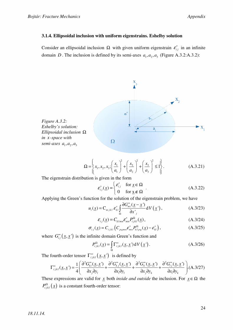
3.1.4. Ellipsoidal inclusion with uniform eigenstrains. Eshelby solution
Consider an ellipsoidal inclusion Ω with given uniform eigenstrain i jε ∗ in an infinite
domain D . The inclusion is defined by its semi-axes 1 2 3, ,a a a (Figure A.3.2:A.3.2):
Figure A.3.2: Eshelby’s solution: Ellipsoidal inclusion Ω in x -space with semi-axes
1 2 3, ,a a a
22 2
31 21 2 3
1 2 3
, , ; 1xx x
x x xa a a
Ω = + + ≤
. (A.3.21)
The eigenstrain distribution is given in the form
for ( )
0 for x
i ji j
xx
εε
∗∗ ∈Ω
= ∉Ω
. (A.3.22)
Applying the Green’s function for the solution of the eigenstrain problem, we have
( )( ')
( ) C d ''
mi
i m j k l k l
j
G x xu x V x
x
∞
∗
Ω
∂ −=
∂∫ε , (A.3/23)
( ) ( )i j k l mn mn i j k lx C P xε ε ∗ Ω= , (A.3/24)
( )( ) ( )i j i j k l p q m n m n k l p q klx C C P xσ ε ε∗ Ω ∗= − , (A.3/25)
where ( ), 'i jG x x∞ is the infinite domain Green’s function and
( )( ) ( , ') d 'i j k l i j k lP x x x V xΩ ∞
Ω
= Γ∫ . (A.3/26)
The fourth-order tensor ( ), 'i j k l x x∞Γ is defined by
2 2 2 2( , ') ( , ') ( , ') ( , ')1( , ')
4
k i k j l i l j
i j k l
j l i l j k i k
G x x G x x G x x G x xx x
x y x y x y x y
∞ ∞ ∞ ∞
∞ ∂ ∂ ∂ ∂
Γ = + + + ∂ ∂ ∂ ∂ ∂ ∂ ∂ ∂ .(A.3/27)
These expressions are valid for x both inside and outside the inclusion. For x ∈Ω the
( )i j k lP xΩ is a constant fourth-order tensor:
Bojtár: Fracture Mechanics Appendix
25
18.11.14.
3 1 21 2 3
S
( ) ( ) ( )dS ( ), 4
i j k l i j k l i j k l
a a aP x P H a D xξ ξ ξ
πΩ − −= = ∈Ω∫ , (A.3/28)
where i j k lP is the Hill polarization tensor8 and
( ) ( ) ( ) ( ) ( )i j k l i k j l j k i l i l j k j l i kH N N N Nξ ξ ξ ξ ξ ξ ξ ξ ξ ξ ξ ξ ξ= + + + , (A.3/29)
( ) ( ) ( )2 2 2
1 1 2 2 3 3a a a aξ ξ ξ= + + . (A.3/30)
The integration is carried out over the surface of a unit sphere2S in ξ -space (fFigure
A.2.7), where
( )1
2 2 2 21 2 3ξ ξ ξ ξ= + + , (A.3/31)
ξ
ξξ
= . (A.3/32)
Let us introduce a fourth-order tensor
( ) C ( )i j k l mnk l i jmnS x P xΩ= , (A.3/33)
thus the strain and stress field in D can be rewritten as
( ) S ( )i j i j k l k lx xε ε ∗= , (A.3/34)
( ) ( )( ) ( ) ( )i j i j k l k l m n m n k l i j k l k l m n k l m n m nx C S x C S x Iσ ε ε ε∗ ∗ ∗= − = − (A.3/35)
with i j k lI fourth-order identity tensor:
( )1
2i j k l i k j l i l j kI δ δ δ δ= + . (A.3/36)
From equations (A.3/28) and (A.3/33), for x ∈Ω , ( )i j k lS x is also constant, thereby the
total strain and stress field is uniform inside the ellipsoidal inclusion given that the
eigenstrain is uniform:
( ) , i j i j k l k lx S xε ε ∗= ∈Ω . (A.3/37)
The i j k lS fourth-order tensor is the Eshelby inclusion tensor and equation (A.3/37) is
called the Eshelby ellipsoidal inclusion solution. From Hooke’s law, the stress field can
easily be obtained:
( )i j i j k l k l k l i j k l k l i jC Cσ ε ε ε τ∗ ∗= − = + , (A.3/38)
i j i j k l k lCτ ε∗ ∗= − . (A.3/39)
i jτ ∗ indicates the stress polarization, which is the stress inside the inclusion caused by
eigenstrain i jε ∗ when the inclusion is not allowed to deform, that is, the total strain i je
is zero. It is the case, when – in the previous example – the aluminum ball with given
thermal strains was embedded into a rigid matrix.
The Eshelby tensor i j k lS is nonsingular, independent of the eigenstrain but it is
dependent on the material of the matrix. About the symmetry of the tensor, in general
the Eshelby tensor does not possess the diagonal symmetry i j k l k l i jS S≠ , but the minor
symmetry i j k l j i k l i j l k j i l kS S S S= = = always holds. In case of general anisotropic
8 See: Hill, R.: Continuum micro-mechanics of elastoplastic polycrystals, J. Mech. Phys. Solids, 13, pp. 89-101, 1965.
Bojtár: Fracture Mechanics Appendix
26
18.11.14.
materials, the integration in the Eshelby tensor needs to be carried out numerically. For
isotropic materials, the integral can be rewritten as elliptical integrals and for special
shaped inclusions, explicit expressions can be obtained (see Mura [ ]1987 ).
Please note, that Eshelby’s ellipsoidal inclusion solution is only valid for material points
inside the inclusion, hence, when computing the strain and stress field in the surrounding
matrix, one has to carry out the integration in (A.3/26) or it is also convenient to use the
solution based on the uniqueness theorem, namely if we know the elastic field inside the
inclusion, we can compute the jump in the required quantities and we get the solution of
the problem for exterior points. Another solution was obtained by Tanaka and Mura
[ ]1982 . For a given stress field ( )i j Sσ − inside the inclusion, find the stress field
( )i j Sσ + of the exterior points by assuming that Ω is a void and the applied stress is
( )ij Sσ −− . The stress field of the exterior points for the inclusion problem is the sum of
( )ij Sσ − and ( )ij Sσ +
.
A different approach to determine the elastic field of exterior points is to use Green’s functions. In this case, two integrals should be carried out in order to obtain the
associated stress and strain field:
( ) ' d 'x x x xΩ
= −∫ψ , (A.3/40)
1
( ) d ''
x xx x
Ω
=−∫φ . (A.3/41)
Norman Macleod Ferrers [ ]1877 and Frank Watson Dyson [ ]1891 expressed the above
integrals in terms of the following elliptic integrals (the so-called I-integrals):
1 2 3
d( ) 2
( )
sI a a a
s
∞
=∆∫λ
λ π , (A.3/42)
( )1 2 3 2
d( ) 2
( )i
i
sI a a a
a s s
∞
=+ ∆∫
λ
λ π , (A.3/43)
( )( )1 2 3 2 2
d( ) 2
( )i j
i j
sI a a a
a s a s s
∞
=+ + ∆∫
λ
λ π , (A.3/44)
where
( )( )( )( )1
2 2 2 21 2 3
( )s a s a s a s∆ = + + + (A.3/45)
and λ is the largest positive root of the equation
( ) ( ) ( )
22 2
31 2
2 2 2
1 2 3
1xx x
a a aλ λ λ+ + =
+ + +. (A.3/46)
For interior points, 0λ = . In order to define the elastic field for both exterior and interior
points, one must compute the higher order derivatives of (A.3/40) and (A.3.41). If the
I-integrals are applied, due to the fact, that the lower bound of the integrals (A.3/42)-
(A.3/44) are only a function of x , the derivatives of ( )I λ , ( )iI λ and ( )i jI λ can be
reduced to the derivatives of λ . The I-integrals are given for ellipsoids (see Mura
Bojtár: Fracture Mechanics Appendix
27
18.11.14.
[ ]1987 ), therefore this is the easiest way to determine the elastic field in a material
caused by the presence of inclusions.
3.1.5. Isotropic inclusions
3.1.5.1. Ellipsoidal inclusions with polynomial eigenstrains
Consider an elastic infinite body D with an ellipsoidal inclusion Ω . The eigenstrain on
the inclusion is given in the form
( ) ...i j i j k k i j k l k lx B x B x xε ∗ = + + , (A.3/47)
where , ,...i j k i j k lB B are constants symmetric with respect to the free indices i and j (e.g.
i j k l i j l kB B= ) and the constant term was excluded for the sake of simplicity. The
displacement field of both the interior and exterior points can be expressed with the help
of functions
( ) ' ( ') d 'i j i jx x x x x∗
Ω
Ψ = −∫ ε , (A.3/48)
( ')( ) d '
'
ij
i j
xx x
x x
∗
Ω
Φ =−∫
ε. (A.3/49)
( )i j xΦ and ( )i j xΨ are the harmonic and biharmonic potentials due to a body Ω of
density ( )ij xε ∗. Substituting the polynomial eigenstrain into the potential functions, we
have
( ) ...i j i j k k i j k l k lx B Bψ ψΨ = + + , (A.3/50)
( ) ...i j i j k k i j k l k lx B Bφ φΦ = + + (A.3/51)
with
... ( ) ' ' ' ' d 'i j k i j kx x x x x x xΩ
= ⋅⋅⋅ −∫ψ , (A.3/52)
...
' ' '( ) d '
'
i j k
i j k
x x xx x
x xΩ
⋅ ⋅ ⋅=
−∫φ . (A.3/53)
The harmonic potentials (A.3/52) and (A.3/53) can be expressed in terms of the
following elliptic integrals:
1 2 3
( )( ) d
( )
U sV x a a a s
s
∞
=∆∫λ
π , (A.3/54)
( )1 2 3 2
( )( ) d
( )i
i
U sV x a a a s
a s s
∞
=+ ∆∫
λ
π , (A.3/55)
( )( )1 2 3 2 2
( )( ) d
( )i j
i j
U sV x a a a s
a s a s s
∞
=+ + ∆∫
λ
π , (A.3/56)
where
( ) ( ) ( )
22 2
31 2
2 2 2
1 2 3
( ) 1xx x
U sa s a s a s
= − + + + + +
. (A.3/57)
According to Dyson [ ]1891 the potentials (A.3/52) and (A.3/53) are related to the V-
integrals in the following way:
Bojtár: Fracture Mechanics Appendix
28
18.11.14.
Vφ = , (A.3/58) 2
n N n Na x Vφ = , (A.3/59)
( )( )2 2 21
4mn M m n N MN mn r r R M M r r RMa x x a V V x x V a V x x Vφ δ
= + − − −
.(A.3/60)
The I -integrals (A.3/42)-(A.3/44) and V -integrals (A.3/54)-(A.3/56) are related:
( )1
( ) ( ) ( )2
r r RV x I x x Iλ λ= − , (A.3/61)
( )1
( ) ( ) ( )2
i i r r RiV x I x x Iλ λ= − , (A.3/62)
( )1( ) ( ) ( )
2i j i j r r R i jV x I x x Iλ λ= − . (A.3/63)
Eshelby pointed out in (Eshelby [ ]1961 ) that in case of an eigenstrain which is a
homogeneous polynomial of ix with degree n , the total strain inside the inclusion
becomes an inhomogeneous polynomial of ix with terms of degree ( ) ( ), 2 , 4 ,...n n n− −
The same result was obtained for anisotropic materials by Asaro and Barnett (Asaro –
Barnett, [ ]1975 ). The I-integrals are of great importance in the explicit expressions of
the solutions of special shaped inclusions.
3.1.5.2. Energies of inclusions
Consider a finite body D with homogeneous and isotropic (or anisotropic) material.
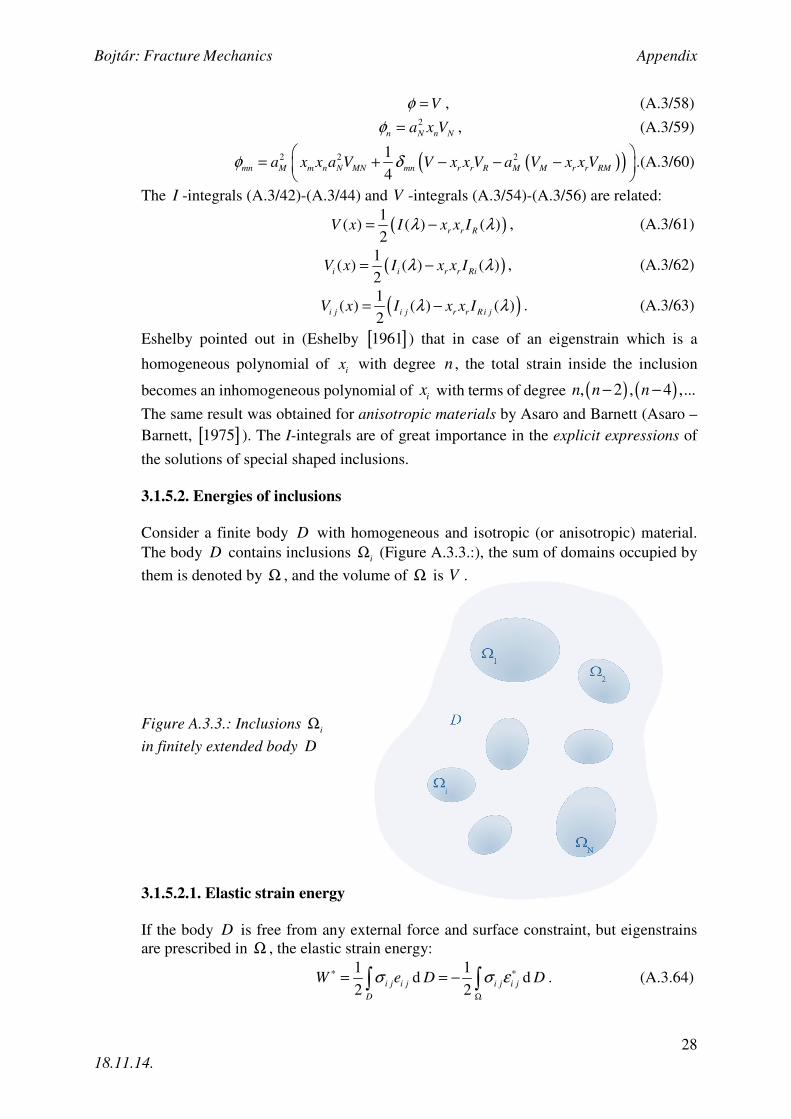
The body D contains inclusions iΩ (Figure A.3.3.:), the sum of domains occupied by
them is denoted by Ω , and the volume of Ω is V .
Figure A.3.3.: Inclusions iΩ
in finitely extended body D
3.1.5.2.1. Elastic strain energy
If the body D is free from any external force and surface constraint, but eigenstrains
are prescribed in Ω , the elastic strain energy:
1 1
d d2 2
i j i j i j i j
D
W e D D∗ ∗
Ω
= = −∫ ∫σ σ ε . (A.3.64)
Bojtár: Fracture Mechanics Appendix
29
18.11.14.
If Ω is an ellipsoidal inclusion and the eigenstrain is uniform, the stress field will also
be uniform, thus the strain energy becomes
1
2i j i jW Vσ ε∗ ∗= − . (A.3/65)
If Ω is the sum of two inclusions 1Ω and 2Ω , the strain energy can be written in the
form
( ) ( )( ) ( ) ( ) ( )( ) ( )
( ) ( ) ( ) ( ) ( ) ( )
1 2
1 2 1
1 2 1 1 2 2
1 1 2 2 2 1
1d d
2
1d d 2 d ,
2
i j i j i j i j i j i j
i j i j i j i j i j i j
W D D
D D D
∗
Ω Ω
Ω Ω Ω
= − + + + =
= − + +
∫ ∫
∫ ∫ ∫
σ σ ε σ σ ε
σ ε σ ε σ ε
(A.3/66)
where ( )1
i jε and ( )2
i jε are the eigenstrains in the first and second inclusion, and ( )1
i jσ and
( )2
i jσ are the stress fields caused by ( )1
i jε and ( )2
i jε , respectively. Then consider the case
when body D is subjected to given surface tractions iF . The displacement field is the
sum of the displacements 0
iu caused by iF only and the displacements iu caused by the
eigenstrains only. The elastic strain energy in this case
( )( )0 0 0 0
, , ,
1 1 1d d
2 2 2i j i j i j i j i j i j i j i j i j
D D
W u u D u dD D∗ ∗ ∗
Ω
= + + − = −∫ ∫ ∫σ σ ε σ σ ε , (A.3/67)
where 0
i jσ is the stress field caused by 0
iu and i jσ is that caused by the eigenstrains.
Please note, that the elastic strain energy is the sum of the energies caused by the
external force and the eigenstrain, respectively, which is a Colonnetti’s theorem9.
3.1.5.2.2. Interaction energy
The total potential energy of a finite body D containing inclusions Ω with external
surface tractions iF on S and eigenstrain i jε ∗ in Ω :
( )0 di i i
S
W W F u u S∗= − +∫ . (A.3/68)
If there is no eigenstrain in D , the total potential energy becomes
0 0 0
0 ,
1d d
2i j i j i i
D S
W u D F u S= −∫ ∫σ . (A.3/69)
If the external forces are zero, the total potential energy of D :
( )1 ,
1 1d d
2 2ij i j i j i j i j
D
W u D D∗ ∗
Ω
= − = −∫ ∫σ ε σ ε . (A.3/70)
The interaction between the traction forces and the eigenstrain appears in the total
potential energy as well. The interaction energy is defined as
0
0 1 d di i i j i j
S
W W W W F u S D∗
Ω
∆ = − − = − = −∫ ∫σ ε . (A.3/71)
9 Colonnetti’s theorem states that if a body containing an inclusion is subjected to traction forces
on its boundary, there will be no cross term in the total elastic energy of the body, between the
internal stress field and the applied stress field. Gustavo Colonnetti (1886 – 1968) was an Italian
mathematician and engineer who made important contributions to continuum mechanics and
strength of materials.
Bojtár: Fracture Mechanics Appendix
30
18.11.14.
In case of uniform eigenstrain in an ellipsoidal inclusion Ω , the interaction energy: 0
i j i jW Vσ ε ∗∆ = − . (A.3/72)
Under constant temperature, the elastic strain energy of a body is the Helmholtz free energy of the body. The Gibbs free energy of a body is the total potential energy of it,
which is defined as the sum of the elastic strain energy of the body and the potential
energy of an external force. 0W is the Gibbs free energy of D when only the external
force is the source of the stress field. 1W is the Gibbs free energy of the body when there
is no external force but there is an internal stress field due to the inclusion. Thus, W∆
is an additional term in the Gibbs free energy when not only an external force acts on
the body, but also there is an eigenstrain-induced stress field in it. It represents the
coexistence of the two effects acting on the body.
For example, in fracture mechanics, we are interested in the energy that is produced in
a body initially subjected to external tractions iF , when due to inclusions, eigenstrain
is introduced in the material as well:
0 1W W W W W∆ = − = + ∆ . (A.3/73)
This energy is formed due to the eigenstrain and the interaction between the inclusions
and the external forces. Please note that all the expressions for energy calculations are
given by integrals over Ω , thus, the calculations become easier.
For dilatational eigenstrains
( )i j i j xε δ ε∗ ∗= , (A.3/74)
the elastic strain energy per unit volume of an inclusion is constant independently of the
shape of the inclusion, and can be expressed in terms of Lamé’s constant µ and
Poisson’s ratio ν of the material under consideration:
( )2 1
21
W
V
νµ ε
ν
∗∗ +
=−
, (A.3/75)
with the volume of Ω :
1 2 3
4
3V a a aπ= . (A.3/76)
As a result, the hydrostatic pressure 3
iiσ is uniform for any shape of inclusion in case of
dilatational eigenstrain − that can be constant or a function of x as well −:
14 in ,
1
0 outside .ii
νµ ε
σ ν∗+
− Ω= − Ω
. (A.3/77)
The stress field inside an inclusion is only a function of the dilatational eigenstrain inside
this particular inclusion, hence in case of several simultaneous inclusions, the
dilatational eigenstrains do not interact. This observation holds only for isotropic
materials and only for inclusions.
Bojtár: Fracture Mechanics Appendix
31
18.11.14.
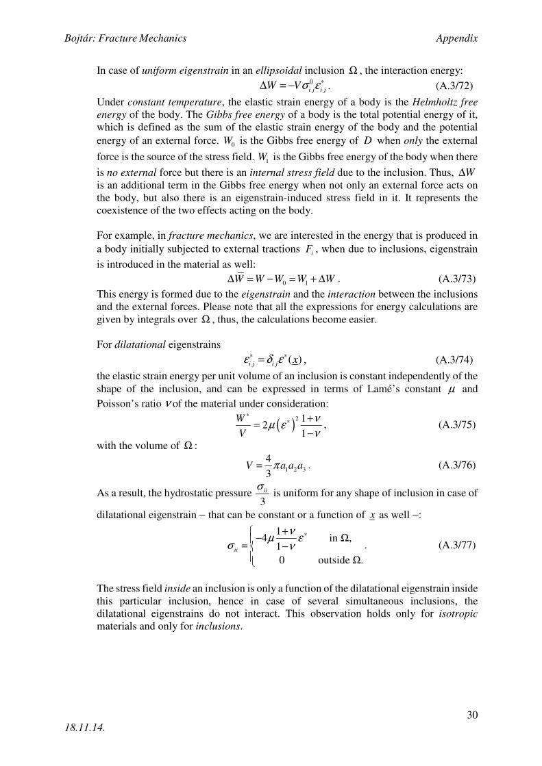
3.1.5.3. Cuboidal inclusions
Cuboidal shaped inclusions (Figure A.3.4.:) are interesting
from that point of view, that the stress field inside the
cuboidal inclusion will not be uniform in case of uniform
eigenstrains. There are also logarithmic singularities in
shear stresses in certain edges and corners of the cuboidal
inclusion when i jε ∗ has no shear strain components.
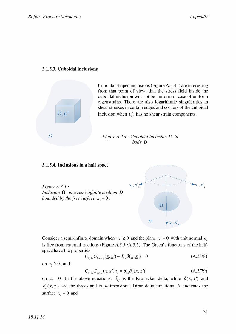
3.1.5.4. Inclusions in a half space
Figure A.3.5.: Inclusion Ω in a semi-infinite medium D bounded by the free surface 3 0x = .
Consider a semi-infinite domain where 3 0x ≥ and the plane 3 0x = with unit normal in
is free from external tractions (Figure A.3.5.:A.3.5). The Green’s functions of the half-
space have the properties
, ( , ') ( , ') 0i j k l k m l j imC G x x x xδ δ+ = (A.3/78)
on 3 0x ≥ , and
, ( , ') ( , ')i j k l k m l j im SC G x x n x xδ δ= (A.3/79)
on 3 0x = . In the above equations, i jδ is the Kronecker delta, while ( , ')x xδ and
( , ')S x xδ are the three- and two-dimensional Dirac delta functions. S indicates the
surface 3 0x = and
Figure A.3.4.: Cuboidal inclusion Ω in body D
Bojtár: Fracture Mechanics Appendix
32
18.11.14.
( ) ( ) ( )0
' , ' d 'f x x x x f xδ∞
=∫ , (A.3/80)
( ) ( ) ( ) ( ) 3' , ' d ' at 0S
S
f x x x S x f x xδ = =∫ , (A.3/81)
( ) ( ), ' , ' 0 if 'Sx x x x x xδ δ= = ≠ . (A.3/82)
The explicit expression for the Green’s function of an isotropic semi-infinite body was
found by Mindlin [ ]1953 . One can look up the formulae in Mura [ ]1987 .
3.1.5.4.1. Ellipsoidal inclusion with a dilatational uniform eigenstrain
The elastic field of the ellipsoidal inclusion with given dilatational uniform eigenstrain
close to the free surface of the half-space (Figure A.3.5.:A.3.5) can be calculated with
the help of the V -integrals (see Mura [ ]1987 ). It was shown by Seo and Mura [ ]1979
that the stresses in the inclusion and the surrounding matrix depends on the shape of the inclusion − sphere or ellipsoid−, and on the depth of the inclusion. Also the uniformity
of the stresses inside the inclusion is mitigated by the existence of the free surface and
tensile stresses may appear in the matrix. The free surface has less effect on the spherical
inclusions, moreover, it was observed that this effect ceases, if the distance between the
free surface and the centroid of the inclusion is greater than the diameter of the sphere.
On the other hand, in case of spherical inclusions, there are large tensile stresses in the
matrix close to the free surface. This behavior diminishes when the inclusion is
embedded deeper in the semi-finite body. These tensile stresses are smaller when
considering ellipsoidal inclusions, but they do not disappear with Ω being deeper in the
matrix.
The elastic strain energy of a semi-infinite body with given dilatational eigenstrain is
extended by a correction factor that represents the effect of free surface. The force acting
on the inclusion is negative, thus the free surface attracts the inclusion.
3.1.6. Anisotropic inclusions
Since explicit expression for Green’s functions of anisotropic materials are not
available, one must carry out the integrals either in the Fourier space or in the physical space.
For any type of eigenstrain distribution in an ellipsoidal shaped inclusion embedded in
an infinitely extended anisotropic material, the resulted elastic field both inside and
outside the inclusion can be calculated from
2
1 2
11 2 3
2
1 0 0
( )
d d d ( ') N ( ) D ( ) '( )dS( )8
i
R
k l m n n m i k l
S
u x
a a az r r C x y z∗ −
−
=
= − −∫ ∫ ∫ ∫π
φ ε ξ ξ ξ δ ζζ ζ ξπ
,(A.3/83)
2
,
1 2
11 2 3
2
1 0 0
( )
d d d ( ') N ( ) D ( ) ''( )d ( )8
i j
R
k l mn nm ik l j
S
u x
a a az r r C x y z S∗ −
−
=
= − −∫ ∫ ∫ ∫π
φ ε ξ ξ ξ ξ δ ζζ ζ ξπ
(A.3/84)
Bojtár: Fracture Mechanics Appendix
33
18.11.14.
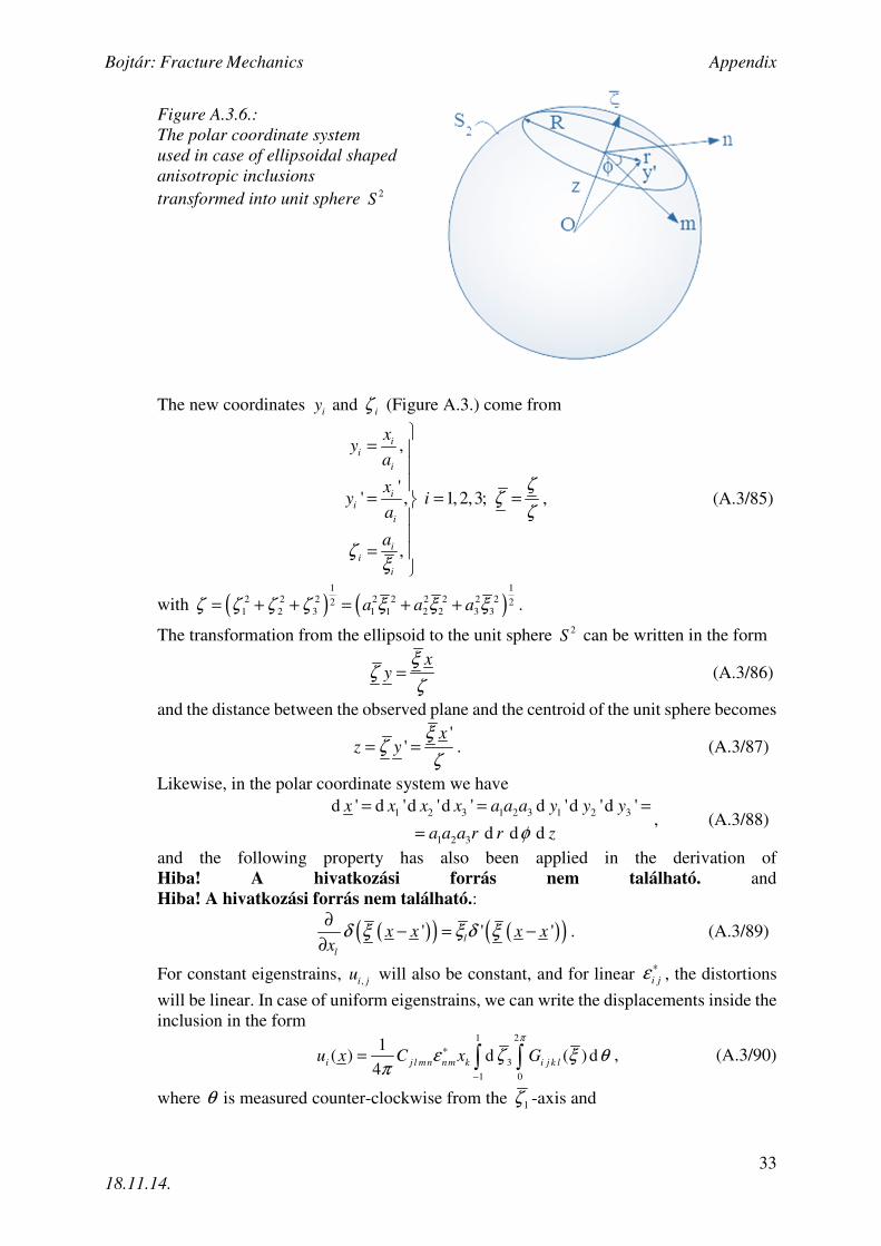
Figure A.3.6.: The polar coordinate system used in case of ellipsoidal shaped anisotropic inclusions
transformed into unit sphere 2S
The new coordinates iy and iζ (Figure A.3.) come from
The transformation from the ellipsoid to the unit sphere 2S can be written in the form
xy
ξζ
ζ= (A.3/86)
and the distance between the observed plane and the centroid of the unit sphere becomes
'
'x
z yξ
ζζ
= = . (A.3/87)
Likewise, in the polar coordinate system we have
1 2 3 1 2 3 1 2 3
1 2 3
d ' d 'd 'd ' d 'd 'd '
d d d
x x x x a a a y y y
a a a r r zφ
= = =
=, (A.3/88)
and the following property has also been applied in the derivation of
Hiba! A hivatkozási forrás nem található. and
Hiba! A hivatkozási forrás nem található.:
( )( ) ( )( )' ' 'l
l
x x x xx
δ ξ ξ δ ξ∂
− = −∂
. (A.3/89)
For constant eigenstrains, ,i ju will also be constant, and for linear i jε ∗
, the distortions
will be linear. In case of uniform eigenstrains, we can write the displacements inside the
inclusion in the form 1 2
3
1 0
1( ) d ( ) d
4i j l mn nm k i j k lu x C x G∗
−
= ∫ ∫π
ε ζ ξ θπ
, (A.3/90)
where θ is measured counter-clockwise from the 1
ζ -axis and
Bojtár: Fracture Mechanics Appendix
34
18.11.14.
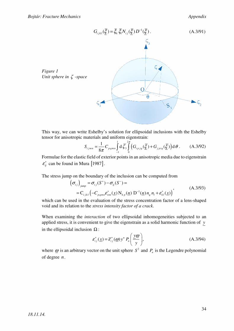
1( ) ( ) ( )i j k l k l i jG N Dξ ξ ξ ξ ξ−= . (A.3/91)
Figure 1 Unit sphere in ζ -space
This way, we can write Eshelby’s solution for ellipsoidal inclusions with the Eshelby
tensor for anisotropic materials and uniform eigenstrain:
( )1 2
3
1 0
1d ( ) ( ) d
8i j m n p q m n i p j q j p i qS C G G
−
= +∫ ∫π
ζ ξ ξ θπ
. (A.3/92)
Formulae for the elastic field of exterior points in an anisotropic media due to eigenstrain
ijε ∗ can be found in Mura [ ]1987 .
The stress jump on the boundary of the inclusion can be computed from
( )
( )1
( ) ( )
C ( ) N ( ) D ( ) ( )
i j i j ijjump
i j k l p qmn nm k p q l k l
S S
C x n n n n x
σ σ σ
ε ε
+ −
∗ − ∗
= − =
= − +, (A.3/93)
which can be used in the evaluation of the stress concentration factor of a lens-shaped
void and its relation to the stress intensity factor of a crack.
When examining the interaction of two ellipsoidal inhomogeneities subjected to an
applied stress, it is convenient to give the eigenstrain as a solid harmonic function of y
in the ellipsoidal inclusion Ω :
( ) ( ) ni j i j n
yx y P
y
ωε ε ω∗ ∗
=
, (A.3/94)
where ω is an arbitrary vector on the unit sphere 2S and nP is the Legendre polynomial
of degree n .
Bojtár: Fracture Mechanics Appendix
35
18.11.14.
References:
Asaro, R. J., – Barnett, D. M. (1975), The non-uniform transformation strain problem
for an anisotropic ellipsoidal inclusion. J. Mech. Phys. Solids (23), pp. 77-83.
Barnett, D. M. (1972), The precise evaluation of derivatives of the anisotropic elastic
Green's functions. Phys. stat. sol.(49), pp. 741-748.
Dyson, F. W. (1891), The potentials of ellipsoids of variable densities. Q. J. Pure and Appl. Math.(25), pp. 259-288.
Gábor, E. (2014), Mechanical Study on the Mesostructure of Heterogeneous Materials,
Student Scientific Work, Budapest University of Technology and Economics, Dep. of Structural Mechanics. Eshelby, J. D. (1951), The force on an elastic singularity. Phil. Trans. Roy. Soc., A244,
pp. 87-112.
Eshelby, J. D. (1957), The determination of the elastic field of an ellipsoidal inclusion,
and related problems. Proc. Roy. Soc., A241, pp. 376-396.
Eshelby, J. D. (1959), The elastic field outside an ellipsoidal inclusion. Proc. Roy. Soc., A252, pp. 561-569.
Eshelby, J. D. (1961), Elastic inclusions and inhomogeneities. (I. N. Sneddon, & R. Hill, Eds.) Progress in Solid Mechanics 2, pp. 89-140. Fazekas F. (1951-68), Exercises of technical mathematics (in Hungarian): B.IV.
Complex functions, Tankönyvkiadó. Ferrers, N. M. (1877), An elementary treatise on spherical harmonics and subjects
connected with them. London: MacMillan and Co.
Gáspár, Gy. – Szarka Z. (1969), Complex functions (in Hungarian). Tankönyvkiadó. Khachaturyan, A. G. (1967), Some questions concerning the theory of phase
transformations in solids. Sov. Phys. Solid State(8), pp. 2163-2168. Kober, H. (1952), Dictionary of Conformal Representations, Dover.
Mindlin, R. D. (1953), Force at a point in the interior of a semi-infinite solid.
Midwestern Conf., Solid Mech., (pp. 56-59).
Mura, T. (1964), Periodic distribution of dislocations. Proc. Roy. Soc., A280, pp. 528-544. Mura, T. (1987), Micromechanics of defects in solids. Dordrecht: Martinus Nijhoff Publishers. Mura, T. – Kinoshita, N. (1971), Green's functions for anisotropic elasticity. Phys. stat. sol.(47), pp. 607-618.
Sadd, M.H. (2005), Elasticity – Theory, Applications and Numerics, Elsevier. Seo, K., – Mura, T. (1979), The elastic field in a half space due to ellipsoidal inclusions
with unifrom dilatational eigenstrains. J. Appl. Mech., 46, pp. 568-572. Tanaka, K., – Mura, T. (1982), A theory of fatigue crack initiation at inclusions.
Metall. Trans.(13A), pp. 117-123.
Willis, J. R. (1975), The interaction of gas bubbles in an anisotropic elastic solid. J.