Fracture toughness and crack resistance curves for fiber compressivefailure mode in polymer composites under high rate loading

Kuhn, P., Catalanotti, G., Xavier, J., Camanho, P. P., & Koerber, H. (2017). Fracture toughness and crackresistance curves for fiber compressive failure mode in polymer composites under high rate loading. CompositeStructures, 182, 164-175. https://doi.org/10.1016/j.compstruct.2017.09.040

Published in:Composite Structures

Document Version:Peer reviewed version

Queen's University Belfast - Research Portal:Link to publication record in Queen's University Belfast Research Portal

Publisher rightsCopyright 2017 Elsevier.This manuscript is distributed under a Creative Commons Attribution-NonCommercial-NoDerivs License(https://creativecommons.org/licenses/by-nc-nd/4.0/), which permits distribution and reproduction for non-commercial purposes, provided theauthor and source are cited.

General rightsCopyright for the publications made accessible via the Queen's University Belfast Research Portal is retained by the author(s) and / or othercopyright owners and it is a condition of accessing these publications that users recognise and abide by the legal requirements associatedwith these rights.

Take down policyThe Research Portal is Queen's institutional repository that provides access to Queen's research output. Every effort has been made toensure that content in the Research Portal does not infringe any person's rights, or applicable UK laws. If you discover content in theResearch Portal that you believe breaches copyright or violates any law, please contact openaccess@qub.ac.uk.

Download date:10. Apr. 2020

Accepted Manuscript

Fracture toughness and crack resistance curves for fiber compressive failuremode in polymer composites under high rate loading

P. Kuhn, G. Catalanotti, J. Xavier, P.P. Camanho, H. Koerber

PII: S0263-8223(17)32082-2DOI: http://dx.doi.org/10.1016/j.compstruct.2017.09.040Reference: COST 8903

To appear in: Composite Structures

Received Date: 6 July 2017Revised Date: 15 September 2017Accepted Date: 16 September 2017

Please cite this article as: Kuhn, P., Catalanotti, G., Xavier, J., Camanho, P.P., Koerber, H., Fracture toughness andcrack resistance curves for fiber compressive failure mode in polymer composites under high rate loading, CompositeStructures (2017), doi: http://dx.doi.org/10.1016/j.compstruct.2017.09.040

This is a PDF file of an unedited manuscript that has been accepted for publication. As a service to our customerswe are providing this early version of the manuscript. The manuscript will undergo copyediting, typesetting, andreview of the resulting proof before it is published in its final form. Please note that during the production processerrors may be discovered which could affect the content, and all legal disclaimers that apply to the journal pertain.

Fracture toughness and crack resistance curves for fibercompressive failure mode in polymer composites under

high rate loading

P. Kuhna,∗, G. Catalanottib, J. Xavierc,d, P.P. Camanhoc,e, H. Koerbera

aTechnical University of Munich, Department of Mechanical Engineering, Chair for CarbonComposites, Boltzmannstraße 15, 85748 Garching, Germany

bSchool of Mechanical and Aerospace Engineering, Queen’s University Belfast, UnitedKingdom

cINEGI, Institute of Science and Innovation in Mechanical and Industrial Engineering,Rua Dr. Roberto Frias 400, 4200-465 Porto, Portugal

dCITAB, University of Tras-os-Montes e Alto Douro, UTAD, Quinta de Prados, 5000-801Vila Real, Portugal

eDEMec, Faculdade de Engenharia, Universidade do Porto, Rua Dr. Roberto Frias,4200-65 Porto, Portugal

Abstract

This work presents an experimental method to measure the compressive crack

resistance curve of fiber-reinforced polymer composites when subjected to dy-

namic loading. The data reduction couples the concepts of energy release rate,

size effect law and R-curve. Double-edge notched specimens of four different

sizes are used. Both split-Hopkinson pressure bar and quasi-static reference

tests are performed. The full crack resistance curves at both investigated strain

rate regimes are obtained on the basis of quasi-static fracture analysis theory.

The results show that the steady state fracture toughness of the fiber compres-

sive failure mode of the unidirectional carbon-epoxy composite material IM7-

8552 is 165.6 kJ/m2 and 101.6 kJ/m2 under dynamic and quasi-static loading,

respectively. Therefore the intralaminar fracture toughness in compression is

found to increase with increasing strain rate.

Keywords: Fiber-reinforced composites, R-curve, Dynamic fracture, Size

effect

∗Corresponding author. Tel.: +49 8928915096; Fax: +49 8928915097. E-mail address:kuhn@lcc.mw.tum.de (P. Kuhn)

Preprint submitted to Journal of Composite Structures September 15, 2017

1. Introduction

Recently proposed strength analysis methods [1, 2, 3, 4, 5] require the speci-

fication of fracture toughness parameters associated to the main failure modes in

order to predict damage evolution after the material strength has been reached.

The softening laws used in the material models with progressive damage are5

dictated by the crack resistance curves (R-curves) [6] and therefore reliable

experimental methods to measure the fracture toughnesses and corresponding

crack resistance curves are needed.

While well established static test standards and procedures are available

for the interlaminar matrix failure modes [7, 8, 9], no test standards exist to10

measure the intralaminar fracture toughness associated with the longitudinal

failure of fiber-reinforced composites. Pinho et al. [10] suggested Compact Ten-

sion (CT) and Compact Compression (CC) tests to obtain fracture toughness

values for fiber tensile and fiber compressive failure, respectively. However,

the CC test specimen is inadequate to measure the R-curve, since i) the kink15

band onset and propagation is accompanied by secondary damage mechanisms

(e.g. delamination) that are neglected and will results in a exaggerated esti-

mation of the fracture toughness; ii) the crack tip cannot be easily identified;

iii) the tractions within the fracture process zone are not taken into account

properly [11]. Hence only the initiation value for the fiber compressive fracture20

toughness can be measured confidently using the CC specimen. Similar work

has been done by Zobeiry et al. [12], testing CC and over-heigth compact tension

(OCT) specimens with a quasi-isotropic layup. Initiation values for compressive

fracture toughness of polymer composites have also been obtained by Laffan et

al. [13] using a four-point bending configuration. Soutis et al. [14] tested multi-25

directional centre-notched compression specimens with various layups and notch

lengths to investigate the influence of the number of 0◦ plies on the laminate

compressive fracture toughness. To overcome the limitations of the CC test

method, Catalanotti et al. [15] proposed a static test method using double-edge

notched (DEN) specimens and the relation between the size effect law and the30

2

R-curve. In follow-up works, the method was extended to tensile [16] and shear

loading [17] and recently used by Pinto et al. [18] to measure the intralaminar

crack resistance curves at extreme temperatures.

Taking into account that automotive and aeronautical polymer composite

structures are subjected to dynamic loading scenarios (e.g. crash, foreign object35

impact), strain rate effects should be captured by advanced composite material

models to predict initiation and evolution of damage accurately. The strain rate

sensitivity of the stiffness and strength components of polymer composites has

been intensively investigated and reviewed over the last decades [19, 20]. In

addition, the experimental investigation of the dynamic interlaminar fracture40

toughnesses has received significant attention, motivated by the need to un-

derstand the delamination damage within composite laminates after low-energy

impact. Published work on dynamic interlaminar fracture toughness was sum-

marized by Jacob et al. [21], concluding that there is no agreement, either, on

the trend of frature toughness with regard to strain rate or on the best suitable45

experimental and analysis procedure.

In contrast to the interlaminar fracture modes, very little is known regarding

the effect of dynamic loading on the energy intensive intralaminar fiber failure

modes. McCarroll [22] used a servo-hydraulic machine to test carbon-epoxy CT

specimens at cross-head velocities up to 12 m/s. With increasing loading speed,50

a possible small decrease of the intralaminar fiber tensile fracture toughness was

found. However, the range of values was within the scatter of the results.

Therefore, there is the need to develop experimental methods to measure the

intralaminar fracture toughness in a dynamic loading scenario. In the presented

work, the methodology proposed by Catalanotti et al. [15] to measure the55

mode I intralaminar R-curve in compression is extended to the case of dynamic

loading. This approach uses the relations between the size effect law, initially

proposed by Bazant and Planas [23], the energy release rate (ERR) and the

R-curve. The method does not require the optical measurement of crack length,

whose determination is found to be a main source of errors in fracture mechanic60

tests [24], and is particularly critical for high loading rate experiments, where

3

high speed cameras with reduced resolution are used. The dynamic tests are

conducted on a split-Hopkinson pressure bar (SHPB), which is a widely-used

setup for dynamic fracture tests [25]. Following Catalanotti et al. [15], double-

edge notched compression (DENC) specimens are used for the determination65

of the size effect law. This specimen type is well suited for SHPB testing, as

it is found to be nonsensitive to complex wave deflections that might cause

undesirable mixed mode stress state during the loading of the specimen.

2. Analysis scheme

The analysis scheme of this work is based on the relations between the energy70

release rate, the R-curve and the size effect law. According to Bazant and Planas

[23], if the energy release rate is an increasing function of the crack length (the

specimen has a positive geometry) the ERR-curves GI for different specimen

sizes wk, corresponding to the peak loads Puk, are tangent to the R-curve R

(Fig. 1). This relation can be used to measure the intralaminar R-curves of fiber75

reinforced polymers, as shown by Catalanotti et al. [15, 16].

[Figure 1 about here]

The energy release rate GI in a balanced cross-ply laminate (with x and y as

the preferred axes of the material) under tensile or compressive loading normal

to the fracture surface (mode I) reads, for a crack propagating along x [26]:80

GI =1

E

√1 + ρ

2K2I (1)

where E denotes the laminate Young’s modulus (E = Ex = Ey), KI is the stress

intensity factor and ρ is the dimensionless elastic parameter defined as [26]:

ρ =2s12 + s66

2√s11s22

(2)

where slm are the components of the compliance matrix computed in the x− y

coordinate system. The stress intensity factor, KI in Eq. (1), depends on the

4

specimen geometry and can be written for a double edge notched specimen85

(Fig. 2) as [26, 27]:

KI = σ√w√φ(α, ρ) (3)

in which σ is the remote stress, w is the characteristic size of the specimen (see

Fig. 2) and φ(α, ρ) is the dimensionless correction function for geometry and

orthotropy including the shape parameter α = a/w. Replacing Eq. (3) in Eq.

(1), GI yields:90

GI(a+ ∆a) =1

E

√1 + ρ

2wσ2φ

(α0 +

∆a

w, ρ

)(4)

where α0 = a0/w is the initial shape parameter (see Fig. 2) and ∆a is the crack

increment.

[Figure 2 about here]

Since there are not analytical solutions available, φ(α, ρ) can be calculated

numerically by applying the Virtual Crack Closure Technique (VCCT) [28].95

Following [15], a two-dimensional Finite Element Model of the DENC specimen

is built in the commercial software Abaqus [29] using 4-node reduced integration

elements (CPS4R) with assigned elastic properties of the laminate (Fig. 3). The

energy release rate, calculated with the VCCT, is equal to:

GI(a?, ρ) = Ym(a?, ρ)un(a?, ρ)/le (5)

where a? is the crack length of the given FE model, Ym and un are the load100

and the displacement in the y-direction of the nodes m and n, respectively, and

le is the element length in x-direction (see Fig. 3). Replacing GI(a?, ρ) in Eq.

(4) yields φ(α?, ρ). Repeating this calculation for several α? using a parametric

model, and fitting the numerical point using a polynomial fitting function allows

the calculation of φ(α, ρ).105

[Figure 3 about here]

The approach proposed by Bazant and Planas [23], that the crack driving

force curve GI at the peak load Pu is tangent to the R-curve R, is described by

5

the following system of equations: GI(∆a) = R(∆a)

∂GI(∆a)∂∆a = ∂R(∆a)

∂∆a .(6)

Using the ultimate nominal stress, σu = Pu/(2wt), where t is the laminate thick-110

ness, and assuming that the size effect law , σu = σu(w), is known, substituting

Eq. (4) in the first of Eq. (6) results in:

1

E

√1 + ρ

2wσ2

uφ

(α0 +

∆a

w, ρ

)= R(∆a) (7)

which holds for every specimen size w. Remembering that, by definition, the

R-curve does not depend on the spezimen size w (∂R/∂w = 0) and assuming

that geometrically similar specimens are tested (α0 is not a function of w) [23],115

the second of Eq. (6) yields:

1

E

√1 + ρ

2

∂

∂w

(wσ2

uφ

(α0 +

∆a

w, ρ

))= 0. (8)

Eq. (8) can be solved for w = w(∆a) and replacing this solution in Eq. (7)

yields the R-curve, R(∆a). Visually, the R-curve is the envelope of the crack

driving force curves at the peak load (see Fig. 1).

The described method provides the R-curve of the laminate. In fiber rein-120

forced polymers the fracture toughness of the fiber failure modes is much higher

than for matrix failure modes that can therefore be neglected [30]. This consid-

eration is also true for interlaminar damage. It should be emphasized that in

the experimental results presented in the following no extensive delamination

was observed; therefore, it can be assumed confidently that the energy dissi-125

pated in the crack propagation is mainly due to the damage of the fiber. Hence,

for a balanced cross-ply laminate, the R-curve of the 0◦ plies, R0(∆a), can be

estimated, from the energy balance, as twice of the laminates R-Curve, R(∆a),

without a significant loss of accuracy [10].

6

3. Material and experimental procedures130

3.1. Material and test specimens

The carbon-epoxy prepreg material system HexPly IM7-8552, which is com-

monly used in primary aerospace structures, was selected for this work. In

accordance with the specified heat cycle [31], a panel with a [0/90]8s layup and

a nominal thickness of 4 mm was cured in a hot press.135

From the manufactured panel, double-edge notched compression (DENC)

specimens were machined using a 1 mm diameter milling tool. A constant

ratio of the geometric properties (length, width, initial crack length a0) was

held for all different specimen sizes (Fig. 4). The dimensions of the specimens

were adopted from [15]. The shape of the initial crack tip does not affect the140

correct determination of the R-curve [16, 32] and was constant (semicircular,

1 mm of diameter) for all specimens. To enable the use of digital image correla-

tion (DIC), the specimens were prepared by applying a random black-on-white

speckle pattern.

[Figure 4 about here]145

Table 1 shows the elastic properties of the laminate under quasi-static (QS)

and high strain rate (HR, εs ≈ 100 s−1) conditions. The Young’s modulus E

and the Poisson’s ratio νxy of the balanced cross-ply were obtained by separate

compression tests with unnotched specimens and no strain rate sensitivity was

found for E. The in-plane shear modulus Gxy was calculated accordingly to the150

classical lamination theory using as reference the values found in [33].

[Table 1 about here]

3.2. Quasi-static experimental setup

The quasi-static (QS) reference tests were carried out on a standard elec-

tromechanical testing machine (Hegewald & Peschke Inspect Table 100), equipped155

with a 100 kN load cell. The tests were conducted under displacement control

7

and a cross-head displacement rate of 0.15 mm/min was imposed. A self align-

ment device as described in [33] was used and friction between the loading parts

and the specimen end-surfaces was minimized by a thin layer of molybdenum

disulphide (MoS2) paste.160

The GOM ARAMIS-4M optical system was used for DIC measurement of

the three-dimensional in plane strain field. It consisted of two CCD cameras

with a resolution of 1728 × 2352 pixel2, adjusted to capture a measuring volume

of 35 × 26 mm2 (length × width). A frame rate of 1 frame per second (fps)

was used together with a shutter speed of 50 ms. Fig. 5 shows the quasi-static165

photomechanical setup.

[Figure 5 about here]

3.3. Dynamic experimental setup

The high strain rate (HR) compression tests were performed on a split-

Hopkinson pressure bar (SHPB) system, as illustrated in Figure 6. The lengths170

of the steel striker-, incident- and transmission bars were 0.6, 2.6 and 1.3 m,

respectively. The strain gauges on the incident-bar were located at 1.3 m and on

the transmission bar at 0.3 m away from the bar-specimen interfaces. The bars

diameter db (Table 2) was adapted to the particular tested specimen width and

friction between the specimen and the bar end-faces was reduced by applying a175

thin layer of MoS2 paste. To ensure that the axial strain rate was the same for

every specimen size, a Finite Element Model was used to set the SHPB configu-

ration in terms of the striker velocity vs and the diameter dPS and thickness tPS

of the copper pulse shaper (Table 2). Expecting a linear stress-strain behaviour

of the specimens up to failure, a triangular shaped incident-wave is best suited180

to obtain nearly constant strain rates [34, 35]. The accuracy of the used SHPB

system was ascertained by bars-together tests, documented in [36].

For the determination of the two-dimensional strain field using DIC, the

specimen deformation was monitored by a single Photron FASTCAM SA-Z

high speed camera. For all specimens, a frame rate of 300,000 fps with a corre-185

sponding resolution of 256 × 128 pixel2 was chosen.

8

[Figure 6 about here]

[Table 2 about here]

3.4. Data reduction methods

3.4.1. Stress, strain and strain rate190

In the case of the quasi-static tests, the ultimate remote stress σu was cal-

culated by dividing the peak load Pu, measured from the load cell of the testing

machine, by the specimen cross-section As, with As = 2wt.

For the high rate tests the axial stress component of the specimen σs can

be calculated with the classic split-Hopkinson pressure bar analysis (SHPBA)195

[37, 38] by using 1-wave- and 2-wave-analysis:

σs1 =AbAsEbεT (9)

σs2 =AbAsEb(εI + εR) (10)

where Ab is the bar cross-section, Eb is the Young’s modulus of the bar material

and εI , εR, εT are the incident, reflected and transmitted bar strain waves,

respectively. As both terms (Eq. 9, Eq. 10) were used to check and confirm

specimen stress-equilibrium, ultimate remote stress was calculated just from200

Eq. 9. The transmission wave εT in Eq. 9 has a smooth signal and dispersion

effects in εT are small due to the short distance between the bar-specimen

interface and the strain gauge terminal on the transmission bar (0.3 m). Since

the specimen strain εs calculated from SHPBA tends to be over-predicted [39],

specimen strain was obtained for all tests from the DIC Software GOM ARAMIS205

by calculating the nominal engineering strain between two facet points along the

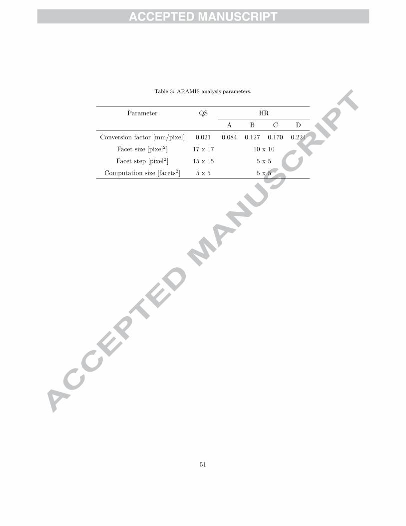
specimen center line, as illustrated in Figure 7. To ensure comparability, the

same procedure was used to estimate the specimen strain in the quasi-static

tests. The DIC analysis parameters were chosen accordingly to the resolutions

of the camera images and are given in Table 3.210

[Figure 7 about here]

9

[Table 3 about here]

The specimen strain was further used to obtain the specimen strain rate εs

in loading direction by applying finite differentiation:

εs(t) =εs(t)− εs(t−∆t)

∆t(11)

in which ∆t is the timestep between two consecutive DIC images.215

3.4.2. Energy terms

The analysis scheme of this work (see section 2) is based on the quasi-

static fracture mechanics theory. According to Jiang and Vecchio [25], quasi-

static fracture theory is applicable for dynamic fracture toughness measurements

under the condition of stress equilibrium. In addition to this classical split-220

Hopkinson bar equilibrium check (using Eq. 9 and Eq. 10), the energy terms of

the specimens were calculated and analyzed by using DIC data. This analysis

procedure therefore uses the true specimen deformation behaviour, obtained

from the optical measurement. According to the law of conservation of energy

for a continuum body, the balance of mechanical energy reads [40]:225

W = U +K (12)

whereW is the external work, which is stored in the structure as strain energy U

and kinetic energy K. When K � U and fracture is the only energy-consuming

process, quasi-static fracture mechanics theory is applicable [23]. Using the in-

plane strain vector obtained from DIC, the strain energy of the specimen U

is the sum of the strain energy at each individual facet point Uj and can be230

calculated as:

U =∑j

Uj =∑j

Vj1

2(Exε

2xj + Eyε

2yj +Gxyγ

2xyj) (13)

in which εxj , εyj and γxyj are the individual facet’s transversal, longitudinal

and shearing strain, respectively. Vj is the associated volume of the individual

facet point, regulated by the DIC analysis parameters (Table 3) and specimen’s

10

thickness. The kinetic energy of the specimen K is calculated accordingly on235

basis of the velocity field from DIC:

K =∑j

Kj =∑j

1

2DVj(v

2xj + v2

yj) (14)

where vxj and vyj are the individual facet’s transversal and longitudinal velocity,

respectively, and D is the density of the laminate.

4. Experimental results

4.1. Specimen deformation and failure240

For each specimen type and strain rate regime, three valid tests are per-

formed. All specimens fail due to compressive fracture along the direction of

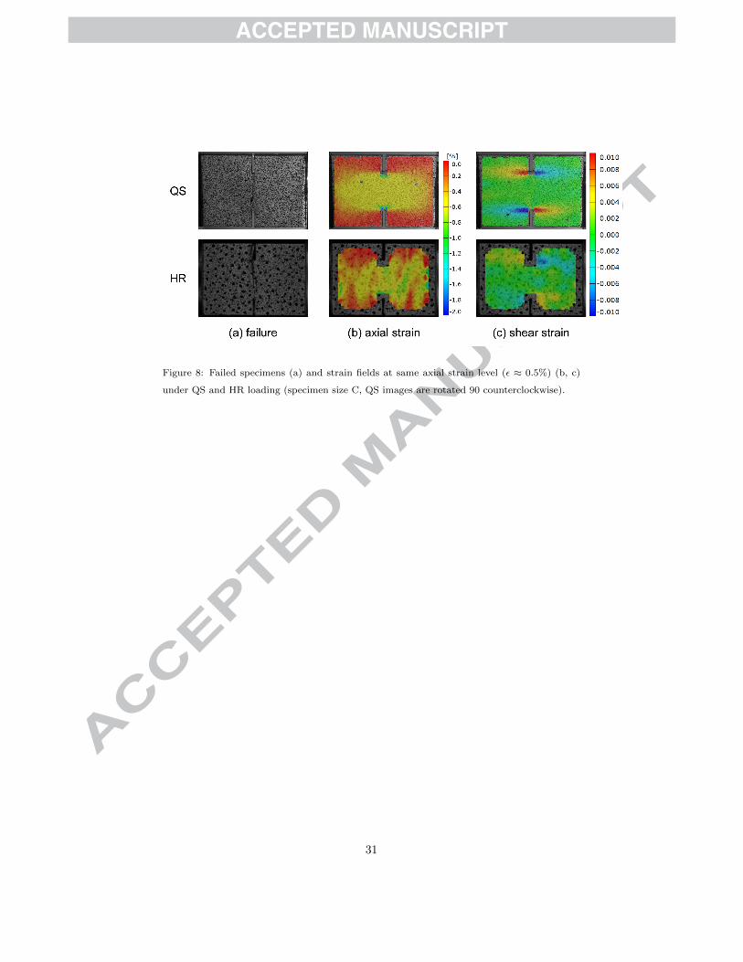
the initial notch, as shown in Fig. 8(a) for two specimens of type C. The ax-

ial (Fig. 8(b)) and shear strain fields (Fig. 8(c)) show plausible axis-symmetric

and point-symmetric strain distributions, respectively, indicating well aligned245

loading of the specimens. Good accordance can be found between the strain

distributions at quasi-static and dynamic loading conditions, which denote that

no complex stress state is caused in the dynamically tested specimens due to

wave deflections. Particularly, no shear strain is detected in the region near

the crack tip at the specimen center, which verifies the assumption of crack250

propagation as a result of mode I loading.

[Figure 8 about here]

4.2. Stress-strain behaviour

Fig. 9 shows representative stress-strain curves for the different specimen

sizes, tested at QS strain rate level (see Appendix A for all stress-strain curves).255

Nearly linear elastic behaviour is detected until the specimens failed by ultimate

compressive failure at peak load.

[Figure 9 about here]

11

In Fig. 10, characteristic bar strain wave groups of a SHPB-test are pre-

sented1. The incident wave shows the desired triangular shape which causes260

a nearly constant strain rate in the specimen, indicated by the plateau in the

reflected strain wave signal [38]. The point of the specimen’s ultimate failure

is expressed by a sharp rise of εR and, as the transmitted wave is proportional

to the stress in the specimen (Eq. 9), by a sharp drop of εT , respectively. The

bar strain waves are used to verify dynamic equilibrium of the specimen, by265

calculating and comparing the 1-wave (Eq. 9) and the 2-wave (Eq. 10) stress-

time signals, plotted in Fig. 11. Despite the existence of small oscillations in

the 2-wave stress-time signal, it can be stated that the DENC-specimen is in

dynamic stress equilibrium before the occurrence of ultimate failure. Following

the classic SHPB theory [38], this implies that the specimen stress can be cal-270

culated correctly from the bar strain waves. Furthermore, the existence of the

stress equilibrium enables the use of the quasi-static fracture theory to obtain

the fracture toughness properties [25].

[Figure 10 about here]

[Figure 11 about here]275

Representative stress-strain curves, obtained at the SHPB, are reported in

Fig. 12 for the different specimen sizes (see Appendix A for all stress-strain

curves). The comparison with the stress-strain curves from QS tests (Fig. 9)

shows that the axial stiffness under dynamic loading is equal, but the HR spec-

imens fail at a higher stress and strain level than the QS specimens. The corre-280

sponding strain rate curves for both investigated loading regimes are shown in

Fig. 13. The strain rate of the QS tests is in the order between 2 × 10−5 s−1

and 1 × 10−4 s−1, which is a typical magnitude for quasi-static loading condi-

tions [41]. For the HR tests a nearly constant strain rate of about 100 s−1 was

achieved for all specimen types, allowing a reliable comparison with each other.285

1The chosen specimen type C was used for a number of other figures presented in this

paper: Fig. 10 can be linked to Figs. 11, 12 and 13.

12

[Figure 12 about here]

[Figure 13 about here]

Fig. 14 shows the plot of the ultimate stress σu vs. the specimen size w. As a

results of the size effect, the ultimate stress decreases with increasing specimen

size at both investigated strain rate regimes [23]. Furthermore, a pronounced290

strain rate effect can be measured. Compared to the QS results, the ultimate

stress at εs ≈ 100 s−1 for specimen type A, B, C and D increases by 23%,

35%, 29% and 28%, respectively. Table 4 summarizes the results for the two

investigated strain rate regimes.

[Figure 14 about here]295

[Table 4 about here]

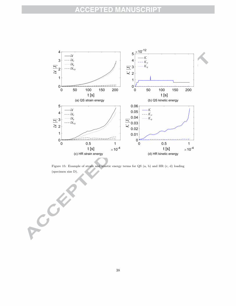
4.3. Energy terms

The terms of strain and kinetic energy, calculated with Eqs. (13) and (14),

are shown exemplarily in Fig. 15 for specimen size D (see Appendix B for en-

ergy terms of other specimen sizes). At both strain rate regimes, strain energy300

increases approximately quadratically over time until ultimate failure occur (at

the last plotted data point). The main part of the overall strain energy U is con-

tributed from the energy portion in loading direction Uy (see Fig. 2). The strain

energy at failure of the HR specimen is higher than for the QS specimen, which

is plausible due to the higher strain at failure at nearly unchanged stiffness (see305

Table 3 and Figs. 9 and 12). Under quasi-static loading, the kinetic energy K

is quite constant at a very low level after initial acceleration (Fig. 15(c)). At

failure, the ratio of U/K is in the order of 1012 and therefore K � U , as char-

acteristic for quasi-static loading. The kinetic energy during dynamic testing is

found to increase over time (Fig. 15(d)). In contrast to an electromechanical310

testing machine, where one specimen interface is at rest while the other is loaded

by the cross-head displacement, both bar-specimen interfaces are in motion at

an SHPB test. The specimen is therefore deformed by the relative displacement

13

between the two interfaces and the kinetic energy in the specimen during SHPB

testing comes partially from the superposed rigid body movement of the DENC-315

specimen. For the HR tests, the ratio of U/K at ultimate failure was calculated

to be 315, 163, 158 and 91 for specimen type A, B, C and D, respectively, and

is therefore significant higher than during the QS tests. However, even in the

worst case (specimen type D), the kinetic energy K is just about 1% of the

strain energy U at failure. Therefore quasi-static fracture mechanics seem to320

be applicable for the analysis of the SHPB-tests without any significant error.

It should be noted that this conclusions is based on the analysis of the overall

specimen deformation behaviour, not taking into account very local effects that

may occur near the crack tip.

[Figure 15 about here]325

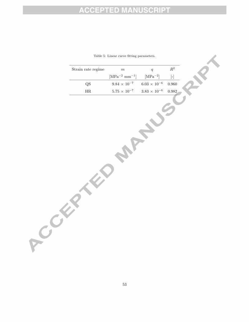
5. Obtaining the Fracture Toughness Properties

According to the analysis scheme (presented in Section 2 of the article), the

size effect law σu = σu(w) must be known to obtain the fracture toughness

properties of the material. To find the relation between the ultimate nominal

stress and the size of the specimen, Bazant and Planas [23] suggested different330

kinds of linear and bilogarithmic regression plots, all leading to very similar

results for the R-curve. For the experimental results of the IM7-8552 DENC

specimens (Section 4), a best fit was obtained for both QS and HR results by

using the following linear regression [23]:

σ−2u = mw + q (15)

in which m and q are the slope and the intercept of the linear curve fit, respec-335

tively. In Fig. 16, σ−2u vs. w and the corresponding linear fitting curves are

plotted for both investigated strain rate regimes. The curve fitting parameters

and the respective coefficient of determination R2 are listed in Table 5.

[Figure 16 about here]

14

[Table 5 about here]340

All parameters of the analysis scheme apart from the size effect law can be

calculated on basis of the material and specimen geometry data (Section 3).

Fig. 17 shows the plot of the dimensionless correction function φ over the shape

parameter α = a/w for the QS and HR material data sets.

[Figure 17 about here]345

With the defined size effect law, the R-curve of the laminate R can be cal-

culated by solving Eq. (8) for w = w(∆a) and substituting this solution in Eq.

(7). Finally, the R-curve of the 0◦ plies R0 is twice the value of R for every

∆a. The R0-curves for both investigated strain rate regimes are presented in

Fig. 18, showing that the compressive intralaminar fracture toughness of the350

0◦ plies under HR loading is considerably larger than that obtained under QS

loading.

[Figure 18 about here]

For the chosen linear regression of the size effect law, the steady-state value

of the fracture toughness R0ss can be calculated as [23]:355

R0ss = lim

w→∞R0 =

√2(1 + ρ)

E

φ0

m(16)

where φ0 = φ|α=α0. The length of the fracture process zone lfpz in case of linear

regression is [23]:

lfpz =f0

2f ′0

q

m(17)

where f0 =√φ|α=α0

and f ′0 = ∂√φ/∂α|α=α0

. The values obtained for R0ss and

lfpz are summarized in Table 6. Table 6 also includes the corresponding coef-

ficients of variation (CV), that are calculated according to Bazant and Planas360

[23] under additional consideration of the Young’s modulus deviation.

[Table 6 about here]

15

The steady-state value of the fracture toughness R0ss under HR loading

(RHRss = 165.6 kJ/m2) is found to be 63% higher than the QS value (RQSss =

101.6 kJ/m2). Despite the fact that the same composite material was used, the365

measured RQSss value measured in the present workis higher than the value cal-

culated with the same procedure by Catalanotti et al. [15] (R0ss = 61 kJ/m2).

However, a lower value for the laminate Young’s modulus for IM7-8552 was used

in the presented work, which has a significant influence on RQSss according to

Eq. (16). It should further be noted, that initiation values of 47.5 kJ/m2 and370

25.9 kJ/m2, measured with compact compression [11] and four-point bending

specimens [13], respectively, represent just single points on the rising part of the

R0-curve.

As for R0ss, the calculated values for the length of the fracture process zone

lfpz also indicate a strain rate effect, however the values are within the scatter375

of the results.

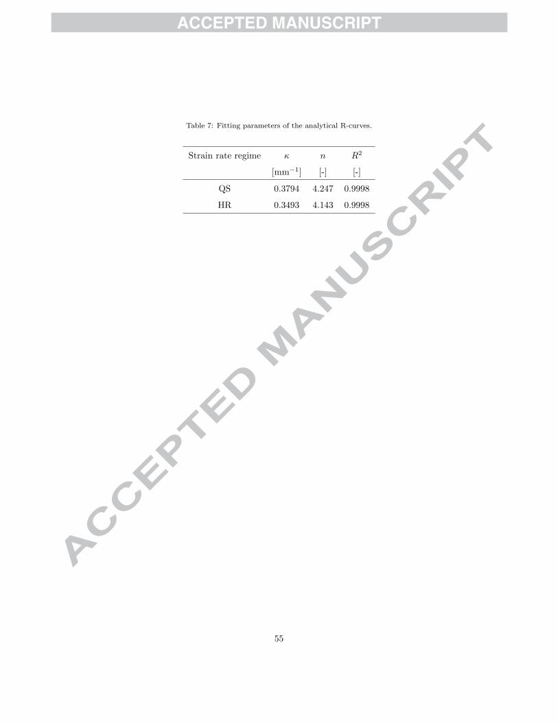
To simplify the use of the measured R-curves, Bazant and Planas [23] rec-

ommend to express them in an analytical form by using the following equation: R0 = Rss [1− (1− κ∆a)n] if∆a < lfpz

R0 = Rss if∆a ≥ lfpz(18)

in which κ and n are the parameters to fit the points obtained by solving Eqs.

(7) and (8). The optimal parameters for both investigated strain rate regimes380

are listed in Table 7.

[Table 7 about here]

6. Conclusions

The presented work shows that the R-curve for the fiber compressive fail-

ure mode can be reliably measured for dynamic loading conditions, using the385

relations between the size effect law, the energy release rate and the R-curve.

It can be concluded, that the used double-edged notched specimens are well

suitable for dynamic tests on a split-Hopkinson pressure bar setup. No signifi-

cant difference could be found between the strain distributions, obtained from

16

DIC, at quasi-static and high rate tests and the assumption of mode I could be390

verified for both investigated strain rate regimes. Furthermore, the DIC data

enabled the calculation and comparison of the strain energy and kinetic en-

ergy terms, indicating that quasi-static fracture theory can be used without any

significant error. In addition, stress equilibrium and a nearly constant strain

rate of about 100 s−1 was achieved for all tested specimen sizes at the SHPB,395

ensuring a reliable determination of the size effect law.

For the investigated carbon-epoxy material IM7-8552, the R-curve for fiber

compressive failure under high rate loading is increased compared to the quasi-

static R-curve. The steady-state value of the fracture toughness under dynamic

loading is 165.6 kJ/m2 and therefore 63% higher than the quasi-static value400

of 101.6 kJ/m2. The length of the fracture process zone also increases from

2.05 mm to 2.24 mm with increasing strain rate.

The results of the presented work contribute to a further understanding of

the complex material response of polymer composite materials. It can be used

to further enhance state-of-the art composite material models and therefore con-405

tributes to a more effective use of composite materials in primary automotive

and aeronautical structures, where dynamic load scenarios must be considered

during the design phase. With the presented results and earlier research pub-

lished by the authors [33, 34, 42], a comprehensive dynamic material data set

for the carbon-epoxy material IM7-8552 now exists.410

Acknowledgements

The authors would like to acknowledge Dr. Iman Taha and Christina Aust

from Fraunhofer Institution for Casting, Composite and Processing Technology

(IGCV) for providing the Photron FASTCAM SA-Z high speed camera. The

presented research did not receive a specific grant from funding agencies in the415

public, commercial, or not-for-profit sectors.

17

Appendix A. Stress-strain curves

The stress-strain curves of the specimen sizes A, B, C and D are shown in

Fig. A.1, Fig. A.2, Fig. A.3 and Fig. A.4, respectively.

[Figure A.1 about here]420

[Figure A.2 about here]

[Figure A.3 about here]

[Figure A.4 about here]

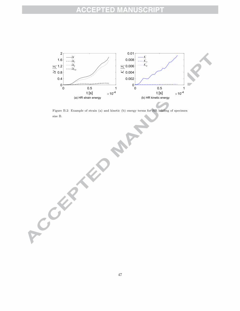
Appendix B. Energy terms

Fig. B.1, Fig. B.2 and Fig. B.3, show energy terms of specimen sizes A, B425

and C, respectively (for specimen size D see Fig. 15).

[Figure B.1 about here]

[Figure B.2 about here]

[Figure B.3 about here]

References430

[1] Lapczyk I, Hurtado JA. Progressive damage modeling in fiber-reinforced

materials. Composites: Part A 2007;38:2333–2341. doi:10.1016/j.

compositesa.2007.01.017.

[2] Maimı P, Camanho PP, Mayugo JA, Davila CG. A continuum damage

model for composite laminates: Part II - Computational implementation435

and validation. Mechanics of Materials 2007;39:909–919. doi:10.1016/j.

mechmat.2007.03.006.

18

[3] Camanho PP, Bessa MA, Catalanotti G, Vogler M, Rolfes R. Modeling

the inelastic deformation and fracture of polymer composites Part II:

Smeared crack model. Mechanics of Materials 2013;59:36–49. doi:10.1016/440

j.mechmat.2012.12.001.

[4] Williams KV, Vaziri R, Poursartip A. A physically based continuum dam-

age mechanics model for thin laminated composite structures. Interna-

tional Journal of Solids and Structures 2003;40:2267–2300. doi:110.1016/

S0020-7683(03)00016-7.445

[5] Forghani A, Zobeiry N, Poursartip A, Vaziri R. A structural modelling

framework for prediction of damage development and failure of composite

laminates. Journal of Composite Materials 2013;47:2553–2573. doi:10.

1177/0021998312474044.

[6] Davila CG, Rose CA, Camanho PP. A procedure for superimposing linear450

cohesive laws to represent multiple damage mechanisms in the fracture of

composites. International Journal of Fracture 2009;158:211–223. doi:10.

1007/s10704-009-9366-z.

[7] ASTM D5528-13, Standard test method for mode I interlaminar fracture

toughness of unidirectional fiber-reinforced polymer matrix composites,455

ASTM International, West Conshohocken, PA. 2013. doi:10.1520/D5528.

[8] DIN EN 6033, Aerospace series - Carbon fibre reinforced plastics - Test

method - Determination of interlaminar fracture toughness energy - Mode

I - GIC; German and English version EN 6033:2015. 2015.

[9] DIN EN 6034, Aerospace series - Carbon fibre reinforced plastics - Test460

method - Determination of interlaminar fracture toughness energy - Mode

II - G[IIC]; German and English version EN 6034:2015. 2015.

[10] Pinho ST, Robinson P, Iannucci L. Fracture toughness of the tensile and

compressive fibre failure modes in laminated composites. Composites Sci-

19

ence and Technology 2006;66:2069–2079. doi:10.1016/j.compscitech.465

2005.12.023.

[11] Catalanotti G, Camanho PP, Xavier J, Davila CG, Marques AT. Measure-

ment of resistance curves in the longitudinal failure of composites using dig-

ital image correlation. Composites Science and Technology 2010;70:1986–

1993. doi:10.1016/j.compscitech.2010.07.022.470

[12] Zobeiry N, Vaziri R, Poursartip A. Characterization of strain-softening be-

havior and failure mechanisms of composites under tension and compres-

sion. Composites: Part A 2015;68:29–41. doi:110.1016/S0020-7683(03)

00016-7.

[13] Laffan MJ, Pinho ST, Robinson P, Iannucci L, McMillan A. Measure-475

ment of the fracture toughness associated with mode I fibre compressive

failure. In: 14th European Conference on Composite Materials, Budapest,

Hungary; 2010.

[14] Soutis C, Curtis PT, Fleck NA. Compressive failure of notched car-

bon fibre composites. Proceedings: Mathematical and Physical Sciences480

1993;440:241–256.

[15] Catalanotti G, Xavier J, Camanho PP. Measurement of the compressive

crack resistance curve of composites using the size effect law. Composites:

Part A 2014;56:300–307. doi:10.1016/j.compositesa.2013.10.017.

[16] Catalanotti G, Arteiro A, Hayati M, Camanho PP. Determination of485

the mode I crack resistance curve of polymer composites using the size-

effect law. Engineering Fracture Mechanics 2014;118:49–65. doi:10.1016/

j.engfracmech.2013.10.021.

[17] Catalanotti G, Xavier J. Measurement of the mode II intralaminar

fracture toughness and R-curve of polymer composites using a modified490

Iosipescu specimen and the size effect law. Engineering Fracture Mechan-

ics 2015;138:202–214. doi:10.1016/j.engfracmech.2015.03.005.

20

[18] Pinto RF, Catalanotti G, Camanho PP. Measuring the intralaminar crack

resistance curve of fibre reinforced composites at extreme temperatures.

Composites: Part A 2016;91:145–155. doi:10.1016/j.compositesa.2016.495

10.004.

[19] Sierakowski RL. Strain rate effects in composites. Applied Mechanics

Reviews 1997;50:741–761. doi:10.1115/1.3101860.

[20] Jacob GC, Starbuck JM, Fellers JF, Simunovic S, Boeman RG. Strain

rate effects on the mechanical properties of polymer composite materials.500

Journal of Applied Polymer Science 2004;94:296–301. doi:10.1002/app.

20901.

[21] Jacob GC, Starbuck JM, Fellers JF, Simunovic S, Boeman RG. The ef-

fect of loading rate on the fracture toughness of fiber reinforced poly-

mer composites. Journal of Applied Polymer Science 2005;96:899–904.505

doi:10.1002/app.21535.

[22] McCarroll C. High rate fracture toughness measurements of laminated

composites. Ph.D. thesis; Imperial College London; 2011.

[23] Bazant ZP, Planas J. Fracture and size effect in concrete and other qua-

sibrittle materials. CRC Press LLC, Boca Raton, Florida, USA; 1998.510

[24] Laffan MJ, Pinho ST, Robinson P, McMillan A. Translaminar fracture

toughness testing of composites: a review. Polymer Testing 2012;31:481–

489. doi:10.1016/j.polymertesting.2012.01.002.

[25] Jiang F, Vecchio KS. Hopkinson bar loaded fracture experimental tech-

nique: A critical review of dynamic fracture toughness tests. Applied Me-515

chanics Reviews 2009;62:1–39. doi:10.1115/1.3124647.

[26] Suo Z, Bao G, Fan B, Wang TC. Orthotropy rescaling and implications

for fracture in composites. International Journal of Solids and Structures

1990;28:235–248.

21

[27] Bao G, Ho S, Suo Z, Fan B. The role of material orthotropy in fracture520

specimens for composites. International Journal of Solids and Structures

1992;29:1105–1116.

[28] Krueger R. The virtual crack closure technique: History, approach and

applications. Technical Report NASA/CR-2002-211628. Tech. Rep. ICASE

Report No. 2002-10; ICASE, Hampton, Virginia, USA; 2002.525

[29] Dassault Systems. Abaqus Version 6.14-2 Documentation. 2014.

[30] Laffan MJ, Pinho ST, Robinson P, Iannucci L. Measurement of the in

situ ply fracture toughness associated with mode I fibre tensile failure in

FRP. Part II: Size and lay-up effects. Composites Science and Technology

2010;70:614–621. doi:10.1016/j.compscitech.2009.12.011.530

[31] Hexcel Product Data Sheet: HexPly 8552 Epoxy matrix. 2016. URL:

http://www.hexcel.com/user_area/content_media/raw/HexPly_

8552_eu_DataSheet.pdf.

[32] Jackson WC, Ratcliffe JG. Measurement of fracture energy for kink-band

growth in sandwich specimens. In: Proceedings of the 2nd international535

conference on composites testing and model identification, Comptest 2004,

University of Bristol, Bristol, UK; 2004.

[33] Koerber H, Xavier J, Camanho PP. High strain rate characterisation of uni-

directional carbon-epoxy IM7-8552 in transverse compression and in-plane

shear using digital image correlation. Mechanics of Materials 2010;42:1004–540

1019. doi:10.1016/j.mechmat.2010.09.003.

[34] Koerber H, Camanho PP. High strain rate characterisation of unidirec-

tional carbon-epoxy IM7-8552 in longitudinal compression. Composites

Part A 2011;42:462–470. doi:10.1016/j.compositesa.2011.01.002.

[35] Nemat-Nasser S, Isaacs JB, Starrett JE. Hopkinson techniques for dynamic545

recovery experiments. Proceedings: Mathematical and Physical Sciences

1991;435:371–391.

22

[36] Koerber H, Xavier J, Camanho PP, Essa YE, de la Escalera FM. High

strain rate behaviour of 5-harness-satin weave fabric carbonepoxy compos-

ite under compression and combined compressionshear loading. Interna-550

tional Journal of Solids and Structures 2015;54:172–182. doi:10.1016/j.

ijsolstr.2014.10.018.

[37] Kolsky H. An investigation of the mechanical properties of materials at

very high rates of loading. Proc Phys Soc London 1949;Sect. B. 62 (II-

B):676–700.555

[38] G. T. Gray III . Classic split-Hopkinson pressure bar testing. In: ASM

handbook mechanical testing and evaluation; vol. 8. ASM International

Ohio USA; 2000, pp. 462-476.

[39] Gama BA, Gillespie JW. Numerical hopkinson bar analysis: uni-axial

stress and planar bar-specimen interface conditions by design. Tech. Rep.560

ARL-CR-553; Army Research Laboratory, USA; 2004.

[40] Mase GT, Smelser RE, Mase GE. Continuum mechanics for engineers.

CRC Press LLC, Boca Raton, Florida, USA; 2010.

[41] S. Nemat-Nasser . Introduction to high strain rate testing. In: ASM hand-

book mechanical testing and evaluation; vol. 8. ASM International Ohio565

USA; 2000.

[42] Kuhn P, Ploeckl M, Koerber H. Experimental investigation of the failure

envelope of unidirectional carbon-epoxy composite under high strain rate

transverse and off-axis tensile loading. In: 11th International Conference

on the Mechanical and Physical Behaviour of Materials under Dynamic570

Loading, Lugano, Switzerland, 2015; vol. 94. 2015, p. 01040 1–6. doi:10.

1051/epjconf/20159401040.

23

Figures

< <

Δa

GI, R

R-curve

GI|PuGI|Pu

GI|Pu

Figure 1: Crack driving force curves GI for different specimen sizes at respective peak load

Pu and R-curve.

24

Figure 2: Double edge notched compression (DENC) specimen.

25

y

x

w

1.5w

sym.

sym. a*

u

m n

le

Figure 3: Finite element model used for application of VCCT.

26

Figure 4: Used specimen sizes (dimensions in mm), machined and prepared specimen for DIC

measurement (size D).

27

Figure 5: Compression setup for quasi-static tests.

28

strain gauge 1 strain gauge 2specimenpulse shaper

striker-bar incident-bar transmission-bar

vs

high speed camera

lighting

Figure 6: Split-Hopkinson pressure bar (SHPB) setup for dynamic tests.

29

Figure 7: Aramis analysis parameters on DENC-specimen (specimen size D).

30

Figure 8: Failed specimens (a) and strain fields at same axial strain level (ε ≈ 0.5%) (b, c)

under QS and HR loading (specimen size C, QS images are rotated 90 counterclockwise).

31

0s [%]

0 0.2 0.4 0.6 0.8 1

<s [M

Pa]

0

50

100

150

200

250

300

350

400

450

ABCD

Figure 9: Stress-strain response for QS loading.

32

time [s] #10-40 1 2 3 4 5 6 7 8 9

bar

stra

in 0

[-]

#10-3

-1

-0.5

0

0.5

1

0I

0R

0T

incident bartransmission bar

Figure 10: Example of a bar strain wave group of an SHPB test (specimen size C).

33

time [s] #10-40 0.2 0.4 0.6 0.8 1 1.2

<s [M

Pa]

0

50

100

150

200

250

300

350

1-wave stress <s1

, Eq. (9)

2-wave stress <s2

, Eq. (10)

Figure 11: Example of a dynamic stress equilibrium check (specimen size C).

34

0s [%]

0 0.2 0.4 0.6 0.8 1

<s [M

Pa]

0

50

100

150

200

250

300

350

400

450

ABCD

Figure 12: Stress-strain response for HR loading.

35

0s [%]

0 0.2 0.4 0.6 0.8 1

stra

in r

ate

[1/s

]

10-5

10-4

10-3

10-2

10-1

100

101

102

103

QS AQS BQS CQS DHR AHR BHR CHR D

Figure 13: Specimen strain rate curves for QS and HR loading.

36

w [mm]4 6 8 10 12 14

<u [M

Pa]

150

200

250

300

350

400

450

QSHR

Figure 14: Ultimate stress σu vs. specimen size w for QS and HR loading.

37

(a) QS strain energy (b) QS kinetic energy

(c) HR strain energy (d) HR kinetic energy

Figure 15: Example of strain and kinetic energy terms for QS (a, b) and HR (c, d) loading

(specimen size D).

38

w [mm]4 6 8 10 12 14

<u-2

[MP

a-2

]#10-5

0.5

1

1.5

2

2.5

QS experimentsQS linear fitHR experimentsHR linear fit

Figure 16: σ−2u vs. w and linear fitting for QS and HR loading.

39

, [-]0 0.1 0.2 0.3 0.4 0.5 0.6 0.7 0.8 0.9

? [-

]

0

2

4

6

8

10

12

14

QS (; = 6.61)HR (; = 5.24)

Figure 17: Correction function φ vs. specimen size w for QS and HR loading.

40

"a [mm]0 0.5 1 1.5 2 2.5 3

R0 [k

J/m

2]

0

20

40

60

80

100

120

140

160

180

200

QSHR

Figure 18: Compressive R-curve of IM7-8552 for QS and HR loading.

41

Figures Appendix A

(a) (b)

Figure A.1: Stress-strain responses of specimen size A for QS (a) and HR (b) loading.

42

(a) (b)

Figure A.2: Stress-strain responses of specimen size B for QS (a) and HR (b) loading.

43

(a) (b)

Figure A.3: Stress-strain responses of specimen size C for QS (a) and HR (b) loading.

44

(a) (b)

Figure A.4: Stress-strain responses of specimen size D for QS (a) and HR (b) loading.

45

Figures Appendix B575

(a) HR strain energy (b) HR kinetic energy

Figure B.1: Example of strain (a) and kinetic (b) energy terms for HR loading of specimen

size A.

46

(a) HR strain energy (b) HR kinetic energy

Figure B.2: Example of strain (a) and kinetic (b) energy terms for HR loading of specimen

size B.

47

(a) HR strain energy (b) HR kinetic energy

Figure B.3: Example of strain (a) and kinetic (b) energy terms for HR loading of specimen

size C.

48

Tables

Table 1: Elastic properties of the laminate.

Strain rate regime E Gxy νxy ρ

[MPa] [MPa] [-] [-]

QS 67,449 5,068 0.042 6.61

HR 67,126 6,345 0.048 5.24

49

Table 2: Split-Hopkinson pressure bar parameters.

Specimen type w db vs Pulse Shaper dimensions

[mm] [mm] [m/s] [mm]

dPS tPS

A 5 16 8.6 6 1.5

B 7.5 18 9.4 8 1.5

C 10 18 11.0 10 2.0

D 12.5 25 12.2 10 2.0

50

Table 3: ARAMIS analysis parameters.

Parameter QS HR

A B C D

Conversion factor [mm/pixel] 0.021 0.084 0.127 0.170 0.224

Facet size [pixel2] 17 x 17 10 x 10

Facet step [pixel2] 15 x 15 5 x 5

Computation size [facets2] 5 x 5 5 x 5

51

Table 4: Summary of the experimental results

A B C D

w [mm] 5 7.5 10 12.5

QS σu [MPa] 310 264 253 234

STDV (σu) [MPa] 33 20 3 17

HR σu [MPa] 380 357 325 299

STDV (σu) [MPa] 29 11 6 8

52

Table 5: Linear curve fitting parameters.

Strain rate regime m q R2

[MPa−2 mm−1] [MPa−2] [-]

QS 9.84 × 10−7 6.03 × 10−6 0.960

HR 5.75 × 10−7 3.83 × 10−6 0.982

53

Table 6: Summary of the fracture toughness properties.

Strain rate regime R0ss lfpz

[kJ/m2] [mm]

QS 101.6 2.04

HR 165.6 2.24

54

Table 7: Fitting parameters of the analytical R-curves.

Strain rate regime κ n R2

[mm−1] [-] [-]

QS 0.3794 4.247 0.9998

HR 0.3493 4.143 0.9998

55