FRAMELETS: MRA-BASED CONSTRUCTIONS OF WAVELET FRAMES ... file011126(.tex) (as of ???) TEX’ed at...

011126(.tex) (as of ???) TEX’ed at 11:34 on 27 November 2001

FRAMELETS: MRA-BASED CONSTRUCTIONS OF WAVELET FRAMES

Ingrid Daubechies Bin Han Amos Ron Zuowei ShenPACM Dept. of Math. Sci. CS Department Dept. of Math.

Princeton U. U. Alberta UW - Madison NUSFine Hall, Wash. Rd. Edmonton, Alberta 1210 West Dayton 10 Kent Ridge Cres.Princeton NJ 08544 Canada T6G 2G1 Madison, WI 53706 Singapore 119260

�� !�"�� # �� $�%�� &��&'�"()��&��$�*�� +��(,&��#��)��&-��&'�*��!�.& �

ABSTRACT

We discuss wavelet frames constructed via multiresolution analysis (MRA), with em-phasis on tight wavelet frames. In particular, we establish general principles and specificalgorithms for constructing framelets and tight framelets, and we show how they can beused for systematic constructions of spline, pseudo-spline tight frames and symmetric bi-frames with short supports and high approximation orders. Several explicit examples arediscussed. The connection of these frames with multiresolution analysis guarantees theexistence of fast implementation algorithms, which we discuss briefly as well.

AMS (MOS) Subject Classifications: Primary 42C15, Secondary 42C30

Key Words: unitary extension principle, oblique extension principle, framelets, pseudo-splines, frames, tight frames, fast frame transform, multiresolution analysis, wavelets.

This work was supported by the US National Science Foundation under Grants DMS-9626319, DMS-9872890, DBI-9983114. and ANI-0085984, the U.S. Army Research Officeunder Contracts DAAH04-95-1-0089 and DAAG55-98-1-0443, the Air Force OSR underaward F49620-01-1-0099, the US DARPA under award 5-36261, the US National Instituteof Health, the Strategic Wavelet Program Grant from the National University of Singapore,the NSERC Canada under a postdoctoral fellowship and Grant G121210654, and AlbertaInnovation and Science REE Grant G227120136.


FRAMELETS: MRA-BASED CONSTRUCTIONS OF WAVELET FRAMES

Ingrid Daubechies, Bin Han, Amos Ron, Zuowei Shen

1. Introduction

Although many compression applications of wavelets use wavelet bases, other typesof applications work better with redundant wavelet families, of which wavelet frames arethe easiest to use. The redundant representation offered by wavelet frames has alreadybeen put to good use for signal denoising, and is currently explored for image compression.Motivated by these and other applications, we explore in this article the theory of waveletframes. We are interested here in wavelet frames and their construction via multiresolutionanalysis (MRA); of particular interest to us are tight wavelet frames. We restrict ourattention to wavelet frames constructed via MRA, because this guarantees the existence offast implementation algorithms. We shall explore the ‘power of redundancy’ to establishgeneral principles and specific algorithms for constructing framelets and tight framelets.In particular, we shall give several systematic constructions of spline and pseudo-splinetight frames and symmetric bi-frames with short supports and high approximation orders.Before we state our main results, we start by reviewing some concepts concerning waveletframes and their structure.

1.1. Wavelet frames

Our discussions here concern dyadic systems; more general wavelet frames are discussedin §5.Basic notations: 〈·, ·〉 denotes the standard inner product in L2(IR

d), i.e.,

〈f, g〉 :=

∫

IRd

f(y)g(y) dy,

which can be extended to other f and g, e.g. when fg ∈ L1(IRd). We normalize the

Fourier transform as follows: f(ω) :=∫IRd f(y)e−iω·y dy. Given a function ψ ∈ L2(IR

d), we

set ψj,k : y 7→ 2jd/2ψ(2jy− k). If the function ψi already carries an enumerative index, wewrite ψi,j,k instead.

Let Ψ be a finite subset of L2(IRd). The dyadic wavelet system generated by the

mother wavelets Ψ is the family

X(Ψ) := {ψj,k : ψ ∈ Ψ, j ∈ ZZ, k ∈ ZZd}.

Such a wavelet system X(Ψ) can be used in order to represent other functions in L2(IRd).

Useful in this context is the decomposition operator (known also as the ‘analysis oper-ator’):

T ∗ : f 7→ (〈f, g〉)g∈X(Ψ).

1


The system X(Ψ) is a Bessel system if the analysis operator is bounded, i.e., for someC1 > 0, and for every f ∈ L2(IR

d),∑

g∈X(Ψ)

|〈f, g〉|2 ≤ C1‖f‖2L2(IRd).

For wavelet systems X(Ψ), it is easy to satisfy this basic and natural requirement: if each

of the mother wavelets has at least one vanishing moment, i.e., ψ(0) = 0, for all ψ ∈ Ψ,then X(Ψ) is a Bessel system if the functions in Ψ satisfy some mild smoothness conditions(see e.g. [CS], [RS2]).

A Bessel system X(Ψ) is a frame if the analysis operator is bounded below, i.e., ifthere exists C2 > 0 such that, for every f ∈ L2(IR

d),∑

g∈X(Ψ)

|〈f, g〉|2 ≥ C2‖f‖2L2(IRd).

This imposes more stringent conditions on X(Ψ). A special case is provided by tightframes: this is the case when X(Ψ) is a frame with equal frame bounds, i.e. C1 = C2;after a re-normalization of the g ∈ X(Ψ), one then has

∑

g∈X(Ψ)

|〈f, g〉|2 = ‖f‖2L2(IRd), for all f ∈ L2(IRd).

This tight frame condition is equivalent to the perfect reconstruction property

f =∑

g∈X(Ψ)

〈f, g〉 g, for all f ∈ L2(IRd).

We are interested in the study of wavelet frames that are derived from a multires-

olution analysis (MRA). Although some of our results and observations cover the caseof vector MRA, we shall restrict our attention to the scalar case. We expect that a fulldescription of the vector case will have additional features linked to the more complexanalysis of approximation order (see e.g.[Pl], [PR]). Our scalar MRA setup follows [RS3]and represents an extension of the original MRA setup ([Ma], [Me], [D1]).

Let φ ∈ L2(IRd) be given and let V0 := V0(φ) be the closed linear span of its shifts, i.e.,

V0 is the smallest closed subspace of L2(IRd) that contains E(φ) := {φ(·−k) : k ∈ ZZd}. Let

D be the operator of dyadic dilation: (Df)(y) :=√

2d f(2y), and set Vj := DjV0, j ∈ ZZ.The function φ is said to generate the (stationary) MRA (Vj)j if the sequence (Vj)j isnested:

(1.1) · · · ⊂ V−1 ⊂ V0 ⊂ V1 ⊂ · · · ,

and, if, in addition, the union ∪jVj is dense in L2(IRd). (The MRA condition (1.1) is

equivalent to the inclusion V0 ⊂ V1.) The generator φ of the MRA is known as a scalingfunction or a refinable function. Finally, the MRA is local if it is generated by acompactly supported refinable function. (The MRA condition in [Ma], [Me], [D2] alsorequired that φ and its shifts constitute a Riesz basis of V0, which is not required in [RS3]or here.)

2


(1.2) Definition: MRA constructions of wavelet systems [RS3]. A wavelet system

X(Ψ) is said to be MRA-based if there exists an MRA (Vj)j such that the condition Ψ ⊂ V1

holds. If, in addition, the system X(Ψ) is a frame, we refer to its elements as framelets.

The notions of mother framelets, tight framelets, etc., have then their obvious meaning.

Some historical pointers: The concept of frames was first introduced by Duffin andSchaeffer in [DS]. Examples of univariate wavelet frames can already be found in thework of Daubechies, Grossmann and Meyer, [DGM]; necessary and sufficient conditions formother wavelets to generate frames are implicit in e.g. [Me] and [D2]. Characterizations ofunivariate tight wavelet frames are implicit in the work of Wang and Weiss, [FGWW, HW]An explicit characterization of tight wavelet frames (in the multivariate case) was obtainedby Han [H]. Independently of these, Ron and Shen gave in [RS3] a general characterizationof all wavelet frames, and specialized this to the case of tight wavelet frames. Furthermore,applying its general theory, [RS3] also provided a complete characterization of all framelets.

Note that [RS3] included a mild decay condition on Ψ in one of its basic theorems (Theorem5.5 of [RS3]); it was then shown by [CSS] that this theorem could also be proved withoutthis decay assumption, effectively removing the decay constraint for all consequent resultsderived from Theorem 5.5 in [RS3], including the characterization of tight frames andframelets. More recently, several articles proved again some of those results without thedecay constraint; see e.g. [Bo], [CH], [P1]. Finally, band limited tight framelets are alsoconstructed by Benedetto and Li in [BL] (also see [BT]).

Several questions arise naturally:(I) Under what conditions (on the MRA (Vj)j and the mother wavelets Ψ) does one

obtain framelets, or, better, tight framelets?(II) Can one construct (tight) framelets from any MRA? In particular, can one construct

framelets from the MRA induced by a univariate B-spline or a multivariate box splineφ?

As to (I), we first briefly review the characterization of framelets given in [RS3]. Forthis, we start with recalling some basic facts from the theory of shift-invariant spaces.Suppose that (Vj)j is an MRA induced by a refinable function φ. Let Ψ = (ψ1, . . . , ψr) bea finite subset of V1 (these ψ` will be our mother wavelets in the MRA-based construction).Then (see [BDR1,2]), there exist 2π-periodic measurable functions τi, i = 1, . . . , r (referredto hereafter as the wavelet masks) such that, for every i,

ψi = (τiφ)(·2).

Moreover, since φ ∈ V1 (by assumption), there also exists a 2π-periodic τ0 (referred to as

the refinement mask) such that φ = (τ0φ)(·/2); this τ0 completely determines φ andtherefore the underlying MRA. For notational convenience, we will occasionally list therefinable function together with the mother wavelets in the parent wavelet vector

F := (ψ0, ψ1, . . . , ψr) := (φ, ψ1, . . . , ψr).

Similarly, we introduce the notation τ := (τ0, . . . , τr) for the combined MRA mask thatcompletely determines F .

3


In all examples considered in this article, the vector τ consists of trigonometric poly-

nomials. In that case the parent vector F is necessarily of compact support. For thedevelopment of the theory, though, we assume only the following milder conditions:

(1.3) Assumptions. All MRA-based constructions that are considered in this article are“assum

assumed to satisfy the following:(a) Each mask τi in the combined MRA mask τ is measurable and (essentially) bounded.

(b) The refinable function φ satisfies limω→0 φ(ω) = 1.

(c) The function [φ, φ] :=∑

k∈2π ZZd |φ(·+ k)|2 is essentially bounded.

Note that the MRA does not determine φ and τ0 uniquely. For example, if α is a 2π-periodic function which is non-zero a.e., and if the function ϕ defined by ϕ(ω) = α(ω)φ(ω)lies in L2(IR

d), then ϕ is refinable with mask t0(ω) = α(2ω)τ0(ω)/α(ω), and generates thesame MRA as φ does. Incidentally, this remark shows that Assumptions (1.3) depend onthe refinable function representing the MRA: for example, this little manipulation couldtransform an unbounded τ0 into a bounded t0.

The characterization in [RS3] of tight framelets involves a special 2π-periodic function Θ:

(1.4) Definition. Let τ = (τ0, . . . , τr) be as above. Set

τ+ := (τ1, . . . , τr), |τ+(ω)|2 :=r∑

i=1

|τi(ω)|2.

Given a combined MRA mask τ and the corresponding wavelet system X(Ψ), define the

fundamental function Θ of the parent wavelet vector by

(1.5) Θ(ω) :=∞∑

j=0

|τ+(2jω)|2j−1∏

m=0

|τ0(2mω)|2.“extraID

The definition of Θ implies the following important identity, (which is valid a.e.):

(1.6) Θ(ω) = |τ+(ω)|2 + |τ0(ω)|2Θ(2ω).“tetrelation

(Note that this identity was not featured in [RS3], it will be crucial in this paper.)In our statements below, we use the following weighted semi-inner product (here w ≥ 0,and u, v ∈ Cr+1):

〈u, v〉w := wu0v0 +r∑

i=1

uivi.

We also need to single out the following set (which is determined only up to a null set):

σ(V0) := {ω ∈ [−π, π]d : φ(ω + 2πk) 6= 0, for some k ∈ ZZd}.The set σ(V0) is the spectrum of the shift-invariant space V0; it is independent of thechoice of the generator φ of V0, and plays an important role in the theory of shift-invariantspaces (cf. [BDR2,3]). The values assumed by τ outside the set σ(V0) affect neither theMRA nor the resulting wavelet system X(Ψ). In almost every example of interest, thespectrum σ(V0) coincides (up to a null set) with the cube [−π, π]d. In particular, wheneverφ is compactly supported, we automatically have σ(V0) = [−π, π]d.

The following characterization of [RS3] answers question (I) for the tight frames:

4


Proposition 1.7 ([RS3]). Assume that the combined MRA mask τ = (τ0, . . . , τr) is“thmtet

bounded. Assume that φ is continuous at the origin and φ(0) = 1. Define Θ as in (1.5).Then the following conditions are equivalent:

(a) The corresponding wavelet system X(Ψ) is a tight frame.

(b) For almost all ω ∈ σ(V0), the function Θ satisfies:

(b1) limj→−∞ Θ(2jω) = 1.(b2) If ν ∈ {0, π}d\0 and ω + ν ∈ σ(V0), then

(1.8) 〈τ(ω), τ(ω + ν)〉Θ(2ω) = 0.“extraIDtwo

This leads to several solutions to question (II) as described below:

1.2. Extension principles

Proposition 1.7 states mathematically how all the masks “work together” to make thewhole family a tight frame. We have one single family of 2d equations ((1.5) and (1.8))that the masks have to satisfy jointly. In practical constructions, this leads to a “sharedresponsibility” which allows more flexibility. In the original construction of compactlysupported orthonormal wavelets [D1], the refinement mask for φ had to satisfy a conjugatequadrature filter (CQF) conditions as well as stability properties. This excluded symmetricor antisymmetric wavelets, as well as spline wavelets (except for Haar wavelet). Manysubsequent constructions sought to remedy this by relaxing some restrictions: in [CDF],symmetry was obtained at the cost of dropping orthogonality; in their construction twocompactly supported dual refinable functions were needed, only one of which could bespline; in [CW] similar non-orthogonal dual symmetric, spline wavelet bases were given,but only one of them could be compactly supported; in [DGH], symmetry, orthonormalityand compact support were combined at the price of having multiwavelets, or vector MRA;in [DGH], it was shown that this could be done with spline vector MRA. In this paper, weare relaxing the non-redundancy condition, which makes it possible to start from refinableφ that satisfy no other conditions than those in Assumptions 1.3.

At first sight, it is not clear how to use Proposition 1.7 for the practical constructionof tight framelets; one needs to select simultaneously the combined MRA mask τ and thefundamental MRA function Θ, making sure that they satisfy the requirements (1.5) and(1.8); and this is nontrivial to solve. The problem simplifies drastically when one restrictsto the case Θ = 1 on σ(V0), the choice made in [RS3].

Proposition 1.9: The Unitary Extension Principle (UEP), [RS3]. Let τ be the“thmuep

combined MRA that satisfies Assumptions (1.3). Suppose that, for almost all ω ∈ σ(V0),and all ν ∈ {0, π}d,

(1.10)r∑

i=0

τi(ω)τi(ω + ν) =

{1, ν = 0,0, otherwise.

“uprin

Then the resulting wavelet system X(Ψ) is a tight frame, and the fundamental function Θequals 1 a.e. on σ(V0).

5


The proof of the UEP in [RS3] is based on Proposition 1.7. A ‘stand-alone’ proof of theUEP can be obtained by following the arguments we use in the proof of Lemma 2.4 of thecurrent article. The UEP was then used in [RS3] as follows: Given τ0, identify τ1, . . . , τrsuch that the “unitarity condition” (1.10) holds, thus obtaining a tight wavelet frame.Note that when (1.10) holds,

∑ν∈{0,π}d |τ0(ω + ν)|2 ≤ 1 for almost every ω. Therefore,∑

ν∈{0,π}d |τ0(ω + ν)|2 ≤ 1 is a necessary condition to use the UEP.

The UEP proved to be a very useful tool to construct tight framelets, including uni-variate compactly supported spline tight frames [RS3,6], multivariate compactly supportedboxlets, [RS5], and various other tight framelets and bi-framelets in [RS6]. On a moretheoretical level, this extension principle was used in [GR] in order to construct, for anydilation matrix and any spatial dimension, compactly supported tight frames of arbitrarilyhigh smoothness. Recently, the UEP was used in [CH], [P1,2] and [S] in the context ofunivariate strongly local constructions of framelets. We revisit these latter constructionsat the end of this section.

However, these constructions have limitations. In all the constructions of splineframelets listed above, at least one of the wavelets has only 1 vanishing moment, andnone of these frames has approximation order higher than 2. In this paper, we show howto overcome or circumvent these shortcomings. One option is to change the underlyingMRA. In [RS3–6], spline MRAs were used; by leaving the spline framework, considering“pseudo-splines” as in §3.1 below, the same approach as in [RS3–6] leads to tight waveletframes (bi-framelets) with higher approximation order, and with very short support. Thiswas also discovered, simultaneously and independently, in [S] (see §4 of that paper). An-other approach is to revisit Proposition 1.7 and extract more flexible construction rules.To replace the UEP, we formulate the more general Oblique Extension Principle or OEP,as another consequence of Proposition 1.7:

Proposition 1.11: The Oblique Extension Principle (OEP). Let τ be the combined“thmoep

mask of an MRA that satisfies Assumptions (1.3). Suppose that there exists a 2π-periodicfunction Θ that satisfies the following:

(i) Θ is non-negative, essentially bounded, continuous at the origin, and Θ(0) = 1.

(ii) If ω ∈ σ(V0), and if ν ∈ {0, π}d is such that ω + ν ∈ σ(V0), then

(1.12) 〈τ(ω), τ(ω + ν)〉Θ(2ω) =

{Θ(ω), if ν = 0,0, otherwise.“genext

Then the wavelet system X(Ψ) defined by τ is a tight wavelet frame.

There are several ways in which Proposition 1.11 can be proved. One approach is tobuild, like for Proposition 1.9, a stand-alone proof by copying the arguments for Lemma2.4. Another approach is to follow the proof of Corollary 5.3: to show that the Θ hereis the fundamental function associated with τ , and then to invoke Proposition 1.7. Thisalso shows, incidentally, that the existence of Θ satisfying (i) and (ii) is also a necessarycondition for X(Ψ) to be a tight frame. It is more surprising that Proposition 1.11 canalso be derived from Proposition 1.9:

6


Proof: Setting ϑ := Θ1/2, we define a function ϕ via ϕ := ϑφ. Since ϑ is bounded,ϕ lies in L2(IR

d). Consider the combined mask t with

t0 :=ϑ(2·)τ0ϑ

, ti :=τiϑ, i > 0.

From (1.12), we obtain that |t(ω)|2 = 1, a.e. on σ(V0), hence t is well-defined and bounded,and t0 is the refinement mask of ϕ. Moreover, since Θ(0) = 1, we obtain that ϕ iscontinuous at 0 and ϕ(0) = 1. Apply now Proposition 1.9 to t, and observe that thetight wavelet frame obtained from the combined vector t is the same as the wavelet systeminduced by the combined vector τ .

We thus see that Proposition 1.9 and Proposition 1.11 are equivalent. It follows thatevery OEP construction can be obtained also from the UEP, and vice versa, by replacing thegenerator of the MRA by another (carefully chosen) generator of the same MRA. Althoughthe UEP construction suffices, in principle, to construct all MRA-based tight waveletframes, the OEP greatly facilitates the search for new constructions in practice. Indeed,by choosing Θ and τ to be trigonometric polynomials that satisfy the OEP conditionswe naturally obtain a local tight wavelet frame. If we attempt to construct the samesystem by the UEP, then the refinable function is generally not compactly supported, thecorresponding masks are not trigonometric polynomials, and it is impossible to predictwhen we nevertheless will still obtain compactly supported mother wavelets.

Moreover, as we shall see in §3, constructing the τi’s and Θ simultaneously is lessdaunting than it looks. Given τ0, one needs to choose Θ and τi such that (1.12) holds.More explicitly, given a (trigonometric polynomial) τ0 with τ0(0) = 1, we shall identify(trigonometric polynomials) τi and Θ such that the identity (1.12) holds for every ω ∈[−π, π]d and every ν ∈ {0, π}d. Then X(Ψ) will be a local MRA-based tight waveletframe (provided that Θ is non-negative and Θ(0) = 1). We refer to such constructions asstrongly local.

The remainder of this paper is organized as follows:We first elaborate (in §2) on three basic properties of MRA-based wavelet systems:

the approximation order of the underlying MRA, the approximation order of the waveletsystem, and the vanishing moments of the mother wavelets. This analysis allows us tounderstand better the relative merit of various possible constructions.

We then turn our attention (in §3) to several systematic univariate constructions.One effort is directed at constructing refinable functions whose derived frame system has ahigh approximation order. A different effort yields spline frames with high approximationorders. We also discuss briefly general techniques for constructing frames from any givenMRA.

In §4, we give the analysis of the implementation algorithm: the fast framelet trans-

form. Though essentially identical to the widely used fast wavelet transform, the interpre-tation of the results of the framelet transform turns out to be somewhat different.

We conclude this article (§5) with the analysis of wavelet frames that are not neces-sarily tight, or dilations that are not necessarily dyadic, and correspondingly more flexiblecharacterizations. A highlight in this section is the (systematic) construction of univariate(symmetric) spline framelets with optimal approximation order, and very short support;

7


the systems in that construction are always generated by two mother wavelets, and aspecific construction in this class is detailed in §6.

Several authors used the results of [RS3] and obtained UEP-based constructions thatare related to some of ours. Particularly, univariate UEP-based framelet systems thatare generated by 2 or 3 mother wavelets were studied in [CH], [P1,2] and [S]. More re-cently, Chui, He and Stockler completed an independent article [CHS] in which severalresults overlap ours. Neither group of authors was aware of the other’s work before it wascompleted; the two papers are published here consecutively.

2. Approximation orders and vanishing moments for wavelet frames

“Good” wavelet systems are characterized by several desirable properties, which may com-pete with each other. Generally speaking, these properties can be grouped into four cate-gories:

(I): The invertibility and redundancy of the representation. The system is requiredto be orthonormal, or bi-orthogonal, or a tight frame, or a frame. And, there must be afast algorithm that implements the decomposition and the reconstruction.

(II): The space-frequency localization of the system. This is usually measured bythe smoothness of the mother wavelet Ψ and the smoothness of its Fourier transform. IfΨ is compactly supported (or band-limited) one would measure the size of suppΨ (Ψ,respectively).

(III): Approximation properties of X(Ψ). The three pertinent notions here are theapproximation order of the underlying MRA, the number of vanishing moments of themother wavelets, and the approximation order of the system itself. These properties areinvestigated in the current section (for tight framelets), and in §5.2 (for the more generalbi-framelets).

(IV): Miscellaneous properties. Most of these properties are motivated by the ac-tual applications; they include the symmetry of the mother wavelets, the ‘translation-invariance’ of the system, or optimality with respect to certain cost functions.

In this section we concentrate on the approximation properties of the system.

(2.1) Definition: approximation orders and vanishing moments. Let φ be a refin-able function that generates a multiresolution analysis (Vj)j . Let Ψ be a finite collectionof mother wavelets in V1, and let X(Ψ) be the induced wavelet system. We say that:

(a) The refinable function φ (or, more correctly, the MRA) provides approximationorder m, if, for every f in the Sobolev space Wm

2 (IRd),

dist(f, Vn) := min{‖f − g‖L2(IRd) : g ∈ Vn} = O(2−nm).

(b) The wavelet system has vanishing moments of order m0 if, for each mother

wavelet ψ ∈ Ψ, the Fourier transform ψ of ψ has a zero of order m0 at the origin.

8


(c) Assuming that X(Ψ) is a tight frame, we define the truncated representation Qn by

Qn : f 7→∑

ψ∈Ψ,k∈ZZd,j<n

〈f, ψj,k〉ψj,k.

We say that the tight frame X(Ψ) provides approximation order m1 if, forevery f in the Sobolev space Wm1

2 (IRd),

‖f −Qnf‖L2(IRd) = O(2−nm1).

It is customary to label the largest possible number for which these statements canbe made as “the” approximation order of φ or of the MRA, etc.

(2.2) Remarks.(1) Note that the approximation orders provided by φ are completely determined

by the MRA (Vj)j . Thus, two refinable functions that generate the same MRA providethe same approximation order. The study of the approximation order provided by therefinable function φ is a special case of the well-understood topic of the approximation

order of shift-invariant spaces, [BDR1].(2) Since the operator Qn maps into Vn, it is obvious that the approximation order

of the wavelet system cannot exceed the order provided by the MRA. If the system X(Ψ)is orthonormal, the two orders coincide, since then Qn is the orthogonal projector ontoVn, hence ‖f − Qnf‖L2(IRd) = dist(f, Vn) for every f ∈ L2(IR

d). The same is not truefor tight frames. In particular we shall see that, in contrast with the approximation orderprovided by φ (that depends only on the choice of the MRA), the approximation order ofthe wavelet system depends on the choice of the mother wavelets.

In the analysis below, we use the following bracket product, [JM], [BDR1]:

[f, g] :=∑

k∈2π ZZd

f(·+ k)g(·+ k).

We quote briefly some basic results concerning the approximation orders provided by shift-invariant spaces. Given any function φ ∈ L2(IR

d), it is known [BDR1], that φ providesapproximation order m if and only if the function

(2.3) Λφ :=

(1− |φ|

2

[φ, φ]

)1/2

“deflam

has a zero of order m at the origin. Under certain conditions on φ (e.g., if φ is compactly

supported and φ(0) 6= 0), this requirement is equivalent to the Strang-Fix (SF) conditions,

meaning that Λφ has a zero of order m at ω = 0 if and only if ‘φ has a zero of order m

at each k ∈ 2π ZZd \0’ (see [BDR1] for more results and analysis.) If φ(0) = 1, and φ isrefinable with refinement mask τ0, then the SF conditions are implied (but not vice versa)by the requirement that ‘τ0 has a zero of order m at each of the points in {0, π}d\0’.

In this section we explore the connections between the well-understood approximationorder provided by the refinable function on the one hand, and the vanishing moments ofthe mother wavelets, as well as the approximation order of the frame system itself on theother hand. We start by the following lemma, which rewrites Qnf in MRA terms:

9


Lemma 2.4. Let X(Ψ) be an MRA tight frame system and Θ the corresponding funda-“lemqzero

mental function. Then the truncated operator Qn satisfies

Qnf =([f(2n·), φ] φΘ

)( ·2n

), f ∈ L2(IR

d).

In particular, Q0f = [f , φ]φΘ, for every f ∈ L2(IRd).

Proof: We start the proof by observing that

(Q1 −Q0)f =r∑

i=1

∑

k∈ZZd

〈f, ψi,0,k〉ψi,0,k.

As shown in [RS1], this is equivalent to

(2.5) Q1f − Q0f =r∑

i=1

[f , ψi] ψi =r∑

i=0

Θi[f , ψi]ψi −Θ [f , φ]φ,“qone

where ψ0 := φ, Θ0 := Θ and Θi = 1, i = 1, . . . , r. Using the relation

(2.6) ψi = (τiφ)(·/2),“temprel

we further obtain that[f , ψi] =

∑

ν∈{0,π}d

(τiξ)(·2

+ ν),

whereξ := [f(2·), φ] =

∑

k∈2π ZZd

f(2(·+ k))φ(·+ k).

Substituting this into (2.5), invoking again (2.6), and changing the order of the summation,we obtain

Q1f − Q0f = φ(·/2)∑

ν∈{0,π}d

ξ(·/2 + ν)r∑

i=0

Θiτi(·/2)τi(·/2 + ν)− [f , φ] φΘ.

=([f(2·), φ] φΘ

)(·2)− [f , φ] φΘ.

The last equality follows from (1.12) if ω/2 ∈ σ(V0); if ω/2 /∈ σ(V0) it follows from the fact

that φ(ω/2) = 0. (The MRA tight frame must satisfy (1.12) by Proposition 1.7 and (1.6).)Since Qn = DnQ0D−n, we easily conclude that, for every n,

Qnf − Qn−1f =([f(2n·), φ] φΘ

)(·

2n)−

([f(2n−1·), φ] φΘ

)(·

2n−1),

implying, for j < n, Qnf = Qjf−([f(2j ·), φ] φΘ

)( ·2j )+

([f(2n·), φ] φΘ

)( ·2n ). It remains

to show that the sequence (Pjf) defined by

Pjf := Qjf −([f(2j ·), φ] φΘ

)(·2j

)

converges to 0 when j → −∞. This is a simple consequence of the weak compactness ofthe unit ball of L2(IR

d). (See, e.g., [BDR3] for this argument, which uses ∩jVj = {0}.Every MRA automatically satisfies this latter condition, as proved in [BDR3] as well.)

10


The bracket product [φ, φ] and the difference 1−[φ, φ] are known to play a role in MRAanalysis. For instance, the orthogonal projection P0 of f onto V0 satisfies (with the con-

vention that 0/0 := 0) [BDR1], P0f = [f ,φ]

[φ,φ]φ. Clearly, when Θ = 1 and σ(V0) = [−π, π]d,

Q0 = P0 if and only if 1 − [φ, φ] = 0; the latter is a well-known characterization of theorthonormality of E(φ). Lemma 2.4 (as well as Theorem 2.8 below) shows that even when

Θ 6= 1, the difference 1 − Θ[φ, φ] continues to play a central role in the characteriza-tion of the approximation order provided by more general wavelet systems. Even moreto the point, the lemma and theorem connect MRA-based wavelet systems with quasi-

interpolation, [BR]: quasi-interpolation is the art of assigning suitable dual functionals toa given set of ‘approximating’ functions. The fundamental function Θ can be recognizedto be a specific quasi-interpolation rule. Indeed, our proof of Theorem 2.8 below invokesthe following result of Jetter and Zhou concerning quasi-interpolation:

Result 2.7 [JZ1-2]. Let φ, ζ ∈ L2(IRd), and φ(0) 6= 0. Consider the approximation“jz

operators (Qn)n where Qn = DnQ0D−n, and

Q0f = [f , ζ]φ.

Assume that [φ, φ] is bounded. Then (Qn)n provides approximation order m if and onlyif the following two conditions hold:(a) [φ, φ]− |φ|2 = O(| · |2m).

(b) 1− ζφ = O(| · |m).

Theorem 2.8. Let X(Ψ) be an MRA tight frame system and Θ be the corresponding“characao

fundamental function. Assume that Assumptions (1.3) are satisfied; and the underlyingrefinable function provides approximation order m < ∞. Then the approximation orderprovided by the framelet system coincides with each of the following (equal) numbers

(i) min{m,m1}, with m1 the order of the zero of 1−Θ [φ, φ] at the origin.(ii) min{m,m2}, with m2 the order of the zero of Θ−Θ(2·)|τ0|2 at the origin.

(iii) min{m,m3}, with m3 the order of the zero of 1−Θ |φ|2 at the origin.Here, φ is the refinable function, and τ0 is its mask.

Proof: We first prove that the approximation order provided by the frame systemis min{m,m3}, and invoke to this end Result 2.7. In view of Lemma 2.4, our case here

corresponds to the case ζ = Θφ in Result 2.7, hence we need to check the zero orderof [φ, φ] − |φ|2 and of 1 − Θ|φ|2. The latter order is m3. As to the former, since φ isbounded above as well as away of zero in a neighborhood of the origin, the characterizationof the approximation orders provided by φ (cf. [BDR1], or derive it directly from thecharacterization mentioned in the discussion around (2.3)) is given as half the order of the

zero of [φ, φ] − |φ|2 at the origin. Thus, Result 2.7 implies indeed that the frame systemprovides approximation order min{m,m3}.

Assuming φ to provide approximation order m, we obtain (again from either [BDR1]

or directly from the discussion around (2.3)) that, since φ(0) = 1, then, near the origin,

[φ, φ]− |φ|2 = O(| · |2m).

11


In particular,m1 = m3 whenever one of these numbers is< 2m. Consequently, min{m,m1} =min{m,m3}.

Finally, since

(2.9) |τ0|2|φ|2 = |φ|2(2·),“one

we obtain that[Θ−Θ(2·)|τ0|2]|φ|2 = Θ|φ|2 −Θ(2·)|φ(2·)|2.

Since 1−Θ|φ|2 has a zero of exactly order m3 at the origin, 1−Θ|φ|2 = q+ o(| · |m3) nearthe origin where q is some homogeneous polynomial of total degree m3. Hence, near theorigin,

Θ|φ|2 −Θ(2·)|φ(2·)|2 = q(2·)− q(·) + o(| · |m3).

Since q(2·)−q(·) is a nonzero homogeneous polynomial of total degreem3, wheneverm3 > 0

(which is the case, because Θ|φ|2(0) = 1), we see that Θ|φ|2 − Θ(2·)|φ(2·)|2 has a zero ofexactly order m3 at the origin. The conclusion that m2 = m3 now follows from the factthat the order of the zero of [Θ−Θ(2·)|τ0|2]|φ|2 at the origin is exactly m2.

For a given refinable function φ, Theorem 2.8 (iii) suggests that in order to constructtight framelets that provide high approximation order, we should choose Θ as a suitableapproximation, at the origin, to 1/|φ|2. For example, if φ is a B-spline of order m, then

|φ(ω)| =∣∣∣ sin(ω/2)

ω/2

∣∣∣m

. Thus, we should choose Θ as a 2π-periodic function which approxi-

mates the function ∣∣∣∣ω/2

sin(ω/2)

∣∣∣∣2m

at the origin. We shall revisit this issue in §3.3.

(2.10) Discussion: approximation orders vs. vanishing moments. If the behaviors

of Θ and |φ|2 are not “matched” near the origin, then Theorem 2.8 shows that the ap-proximation order of the framelet system can lag significantly behind the approximationorder provided by the refinable function. On the other hand, the approximation order ofthe framelet system turns out to be strongly connected, perhaps in a somewhat surprisingway, to the number of vanishing moments of the wavelets.

Since ψi = (τiφ)(·/2), and since φ(0) = 1, the vanishing moments of ψi are determinedcompletely by the order of the zero (at the origin) of τi. This means that the MRA-basedwavelet system X(Ψ) has vanishing moments of order m0 if and only if |τ+|2 = O(| · |2m0),near the origin. On the other hand, if our system is a tight framelet, it must satisfy theOEP conditions, and thus |τ+|2 = Θ−Θ(2·)|τ0|2. It follows that the index m2 of Theorem2.8 (ii) is exactly equal to 2m0. This proves part of the following theorem:

Theorem 2.11. Let X(Ψ) be an MRA tight frame system. Assume that the system has“momao

vanishing moments of order m0, and that the refinable function φ provides approximationorder m. Then:(a) φ satisfies the SF conditions of order m0, i.e. φ vanishes at each ω ∈ 2π ZZd \0 to order

m0.

12


(b) The approximation order of the tight frame system is min{m, 2m0}.Proof: Because of the remarks above, we need prove only (a).Let ν ∈ {0, π}d\{0}. If X(Ψ) has vanishing moments of order m0, then |τ+|2 =

O(| · |2m0) (near the origin), hence, for every i ≥ 1,

(2.12) τi = O(| · |m0).

Let j ∈ 2π ZZd. Since, thanks to the OEP conditions, 〈τ, τ(·+ ν)〉Θ(2·)φ(·+ ν + j) = 0, (onσ(V0), hence in a neighborhood of the origin), we obtain from (2.12) that Θ(2·)τ0τ0(· +ν)φ(·+ ν + j) = O(| · |m0). Since Θ(0) = τ0(0) = 1, we conclude that

φ(2 ·+2ν + 2j) = τ0(·+ ν)φ(·+ ν + j) = O(| · |m0), ν ∈ {0, π}d\0, j ∈ 2π ZZd .

A routine argument can then be used to prove that the last relation holds for ν = 0 aswell (provided then that j 6= 0).

(2.13) Remark. Part (a) of the above result states, essentially, that the approximationorder provided by φ is ≥ m0. For an MRA-based framelet with exactly m0 vanishingmoments, the approximation order of the framelet is therefore always between m0 and2m0.

In the theory of MRA-based orthonormal wavelets, the approximation order of theMRA, the approximation order of the wavelet system and the number of vanishing momentsof the wavelets are always equal. (Note that this is no longer true for bi-orthogonal bases.)It is therefore customary to inspect only one of those quantities; most of the waveletliterature picks the number of vanishing moments as the focal property.

In contrast, these three parameters need not coincide in the context of framelets. Anatural question then arises: which parameter should we attempt to maximize in actualconstructions? The answer usually depends on the application:

The approximation order of the MRA is clearly important since it provides an upperbound for the approximation order of any framelet system derived from that MRA. Simi-larly, the approximation order of the framelet system is very important since the waveletexpansion must be truncated in any practical implementation. MRAs or framelet expan-sions of low approximation orders transfer to their high frequency scales information aboutthe function/image/signal that could have been faithfully represented in the (sparser) lowfrequency scales of more appropriate framelet expansions.

A further evaluation of the difference between the approximation order of the MRAand that of the framelet system is as follows. The redundancy of the tight framelet systementails that a given f ∈ L2(IR

d) can be represented in many different ways as a convergentsum

(2.14) f =∑

g∈X(Ψ)

c(g) g.“tempo

The tight framelet representation

(2.15) f =∑

g∈X(Ψ)

〈f, g〉 g“temp

13


is one of many. One of its major advantages (over other representations of f as linearcombinations of X(Ψ)) is that it is implemented by a fast transform, the fast frame trans-form. Now, assume that f is, say, a very smooth function. Then, a high approximationorder of the MRA guarantees that some of the (2.14) representations of f are sparse andcompact. Some other (2.14) representations of f may be dense and inefficient. A highapproximation order of the framelet system ensures that the specific representation (2.15)is a good one, i.e., it is (asymptotically) as compact and as effective as the best possible(2.14) representation of f .

It might be worthwhile to mention that not every application requires high approxi-mation orders of the framelet system. For example, in novel image compression algorithmsthat are currently under development, one uses the representation (2.15) as a springboardfor finding the sparsest (2.14) representation of f . In this and similar applications theproperties of the representation (2.15) are less crucial, since this representation is only anintermediate one. More important then is the ability to find a compact representationamong all of those of the type (2.14), and this latter property is more connected to theapproximation order of the MRA itself.

And, what about the impact of vanishing moments? A high number of vanishing mo-ments is important for algorithms that involve the manipulation of the wavelet coefficients.For instance, wavelet representations of one-dimensional piecewise-smooth functions be-come sparser when the number of vanishing moments increases. On the other hand, insome applications, mother wavelets with varying vanishing moments may be preferred,since they can serve, e.g., as ‘multiple detectors’. In other applications, the coefficientsassociated with the mother wavelet that has the highest vanishing moments can be usedto capture the essential information about the object, while the other coefficients simplyaid in the reconstruction process.

Let us illustrate this discussion by comparing several framelets. The first two exam-ples, constructed by an application of the UEP, are borrowed from [RS3]:

Example 2.16 (Figure 1). Take τ0(ω) = (1 + e−iω)2/4. Then φ is the B-spline function“splinetwors

of order 2, i.e. the hat function. Let

τ1(ω) := −1

4(1− e−iω)2 and τ2(ω) := −

√2

4(1− e−i2ω).

The corresponding {ψ1, ψ2} generates a tight framelet. The framelet has m0 = 1 vanishingmoments (though one of the wavelets has 2 vanishing moments); the approximation orderof the MRA is 2. The approximation order of the framelet system equals 2 = min(m, 2m0).

Example 2.17 (Figure 2). Take τ0(ω) = (1 + e−iω)4/16. Then φ is the B-spline function“splinefourrs

of order 4 which is a piecewise cubic polynomial. Let

τ1(ω) := 14 (1− e−iω)4, τ2(ω) := − 1

4 (1− e−iω)3(1 + e−iω),

τ3(ω) := −√

616 (1− e−iω)2(1 + e−iω)2, τ4(ω) := − 1

4 (1− e−iω)(1 + e−iω)3.

The corresponding {ψ1, ψ2, ψ3, ψ4} generates a tight framelet that has vanishing momentsof order m0 = 1. For this φ we have m = 4. The approximation order of the frameletsystem is 2 = min(m, 2m0).

14


0 0.2 0.4 0.6 0.8 1 1.2 1.4 1.6 1.8 2

−0.5

0

0.5

1

0 0.2 0.4 0.6 0.8 1 1.2 1.4 1.6 1.8 2−0.8

−0.6

−0.4

−0.2

0

0.2

0.4

0.6

0.8

Figure 1. The graphs of the wavelet functions ψ1 and ψ2 derived from the B-spline function of order 2 in Example 2.16. {ψ1, ψ2} generates a tightwavelet frame in L2(IR) and has vanishing moments of order 1. Theframelet system provides approximation order 2, which is optimal for apiecewise-linear system.

0 1 2 3 4

−0.5

0

0.5

1

(a)0 1 2 3 4

−0.6

−0.4

−0.2

0

0.2

0.4

0.6

(b)

0 1 2 3 4

−0.2

0

0.2

0.4

(c)0 1 2 3 4

−0.5

0

0.5

(d)

Figure 2. The graphs of the wavelet functions ψ1, ψ2, ψ3, ψ4 derived from the B-spline function of order 4 in Example 2.17; together, the four waveletsgenerate a tight framelet. Wavelet (d) has only one vanishing moment,hence the approximation order is 2, which is suboptimal since the cor-responding MRA provides approximation order 4.

The next two examples are linear, respectively cubic spline framelets constructed byusing the OEP, as described below. We list here τ0, Θ and the τj , and revisit these exampleslater.

15


Example 2.18 (Figure 3). Take τ0(ω) = (1 + e−iω)2/4 and Θ(ω) = (4− cosω)/3. Let“splinetwonew

τ1(ω) := −1

4(1− e−iω)2 and τ2(ω) := −

√6

24(1− e−iω)2(e−iω + 4e−i2ω + e−i3ω).

The set {ψ1, ψ2} generates a tight framelet and has vanishing moments of order 2. Both ψ1

and ψ2 are symmetric and their graphs are given in Figure 3. Even though 2m0 = 4, we stillhave m = 2, so that min(m, 2m0) equals 2; this system has thus the same approximationorder as in Example 2.16.

0 0.2 0.4 0.6 0.8 1 1.2 1.4 1.6 1.8 2

−0.6

−0.4

−0.2

0

0.2

0.4

0.6

0.8

1

0 0.5 1 1.5 2 2.5 3

−0.4

−0.2

0

0.2

0.4

0.6

0.8

1

1.2

Figure 3. The graphs of the symmetric wavelet functions ψ1 and ψ2 derived fromthe B-spline function of order 2 in Example 2.18. {ψ1, ψ2} generatesa tight framelet, and each of the wavelets has two vanishing moments,and hence the approximation order of the system is min{4, 2} = 2; thehigher number of vanishing moments than in Example 2.16 leads tosparser wavelet coefficients but does not improve the decay of the error‖Qnf − f‖ for the truncated reconstruction.

Example 2.19 (Figure 4). Take τ0(ω) = (1 + e−iω)4/16 and“splinefournew

Θ(ω) = 2452/945− 1657/840 cos(ω) + 44/105 cos(2ω)− 311/7560 cos(3ω).

Let

τ1(ω) = t1 (1− e−iω)4[1 + 8e−iω + e−i2ω

],

τ2(ω) = t2 (1− e−iω)4[1 + 8e−iω + (7775/4396 t− 53854/1099)e−i2ω + 8e−i3ω + e−i4ω

],

τ3(ω) = t3 (1− e−iω)4[1 + 8e−iω + (21 + t/8)(e−i2ω + e−i4ω) + t e−i3ω + 8e−i5ω + e−i6ω

],

where t3 =√

32655/20160, t = 317784/7775 + 56√

16323699891/2418025, and

t1 =

√11113747578360− 245493856965 t

62697600, t2 =

√1543080− 32655 t/40320.

16


0 1 2 3 4

0

0.2

0.4

0.6

0.8

(a)0 1 2 3 4 5

−0.2

0

0.2

0.4

(b)

0 2 4 6

−0.5

0

0.5

1

(c)0 2 4 6

−0.4

−0.2

0

0.2

0.4

0.6

0.8

(d)

Figure 4. (b), (c) and (d) are the graphs of the symmetric mother wavelets derivedfrom the cubic B-spline function (a) in Example 2.19. All the motherwavelets have 4 vanishing moments, hence the approximation order ofthe system is min{4, 8} = 4.

The above masks satisfy the OEP conditions, hence lead to a tight framelet. All thewavelets here have 4 vanishing moments hence m0 = 4. The mother wavelets ψ1, ψ2, ψ3

are symmetric. Note that for this φ the approximation order of the MRA is m = 4. Theapproximation order of the framelet system is 4 = min(m, 2m0). The three filters are ofsize 7, 9, 11.

A fifth example is constructed by using the UEP, now starting from a different, non-spline MRA; this construction will also be revisited in more detail in §3.1.

Example 2.20 (Figure 5). In this case we have one scaling function and three wavelets.“fifth

The filters τ0 and τj , j = 1, 2, 3 are obtained by spectral factorization, i.e. by “takinga square root”. In particular, we have |τ0(ω)|2 = cos8(ω/2)

(1 + 4 sin2(ω/2)

), τ1(ω) =

eiωτ0(ω+π), τ2(ω) =√

52 sin2(ω), and τ3(ω) = eiωτ2(ω). The wavelets in this system have

2 vanishing moments, so that m0 = 2. The approximation order of the MRA is m = 4;the approximation order of the framelet is thus min(m, 2m0) = 4.

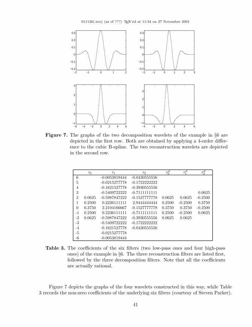
For these five examples, as well as for the bi-framelet of §6, and for three benchmarkwavelet bases (not frames - we used here the Haar basis and the two bi-orthogonal waveletbases known as (5,3) and (9,7)), we provide, for a very smooth function f , the error‖Qnf −f‖, for increasing n. The results are listed in Table 1 (courtesy of Steven Parker ofUW-Madison). For each system we also list three indices in the header of the column: thefirst is the number of vanishing moments of the system, the second is the approximationorder of the system, and the third is the approximation order of the underlying MRA

17


0 1 2 3 4 5

−0.2

0

0.2

0.4

0.6

0.8

(a)−2 −1 0 1 2 3

−0.6

−0.4

−0.2

0

0.2

0.4

0.6

0.8

(b)

0 1 2 3 4

−0.2

0

0.2

0.4

0.6

(c)0 1 2 3 4

−0.2

0

0.2

0.4

0.6

(d)

Figure 5. (b), (c) and (d) are the graphs of the mother wavelets in Example 2.20of the Type I pseudo-spline tight framelets derived from the scalingfunction, pseudo-spline (4, 1), shown in (a). (See §3.1 for details)

HAAR (5,3) (9,7) Ex. 2.16 Ex. 2.17 Ex. 2.18 Ex. 2.19 Ex. 2.20 Bi-framelevel (1,1,1) (2,2,2) (4,4,4) (1,2,2) (1,2,4) (2,2,2) (4,4,4) (2,4,4) (4/2,4,4)

2 6.36e-01 1.57e-01 9.15e-02 3.26e-01 5.62e-01 1.67e-01 5.44e-02 1.93e-01 1.20e-013 3.72e-01 4.83e-02 8.15e-03 1.14e-01 1.86e-01 4.24e-02 9.90e-04 1.64e-02 4.11e-034 1.92e-01 1.27e-02 5.54e-04 3.12e-02 5.01e-02 1.23e-02 3.20e-05 1.11e-03 9.96e-055 9.63e-02 3.20e-03 3.53e-05 7.97e-03 1.28e-02 3.17e-03 2.08e-06 7.12e-05 2.98e-066 4.75e-02 8.02e-04 2.20e-06 2.00e-03 3.20e-03 8.00e-04 1.31e-07 4.47e-06 1.32e-077 2.30e-02 2.00e-04 1.35e-07 5.01e-04 8.00e-04 2.00e-04 8.38e-09 2.80e-07 8.09e-098 1.07e-02 4.94e-05 8.07e-09 1.25e-04 1.98e-04 4.94e-05 5.81e-10 1.75e-08 5.77e-109 4.60e-03 1.18e-05 4.49e-10 3.06e-05 4.71e-05 1.18e-05 4.98e-11 1.09e-09 4.98e-1110 1.53e-03 2.35e-06 2.47e-11 7.06e-06 9.41e-06 2.35e-06 5.54e-12 6.78e-11 5.56e-12

1.07 2.00 3.99 1.96 1.99 2.00 4.08 3.95 4.13

Table 1. The errors ‖Qnf−f‖ for nine different systems, for increasing n (=level);the last row gives the slope of −log2‖Qnf − f‖ as a function of n, com-puted by linear regression.

(the last system is a bi-frame, meaning that the decomposition masks are different fromthe reconstruction masks: the former has four vanishing moments while the latter onlytwo vanishing moments). At the bottom of Table 1 we give the numerical estimate ofthe decay rate of ‖Qnf − f‖ in n; this clearly is (approximately) equal, in all cases, tothe approximation order of the system, and depends only marginally on the other twoindices. Let us look at some particular comparisons. For the linear splines in Examples2.16 and 2.18, the increase in the number of vanishing moments from Examples 2.16 to2.18 does not improve the approximation order of the framelet. What this means is that

18


the estimates of the sizes of the wavelet coefficients, as given by e.g. maxi,k |〈f, ψi,j,k〉|, willdecay faster as j increases for Example 2.18 than for Example 2.16, but that the truncatedwavelet expansions, using coefficients up to level j only, will exhibit comparable errors. Forthe cubic splines in Examples 2.17 and 2.19, the number of vanishing moments increasesfrom 1 (for Example 2.17) to 4 (for Example 2.19); this is reflected by an increase in theapproximation order of the corresponding framelets, from 2 to 4. In Example 2.20 we haveonly 2 vanishing moments, but the framelet approximation order is 4, and the decay of‖Qnf − f‖ is comparable to that for Example 2.19, even though the decay of the waveletcoefficients will be less fast.

Let us proceed now with a more systematic tour.

3. A tour through univariate constructions of tight framelets

We restrict our attention here to strongly local MRA-based constructions. Construc-tions are typically guided by a desire for some of the following properties for the motherwavelets:(i) Short filter/support.(ii) High smoothness.(iii) High approximation orders of the refinable function.(iv) High approximation orders for the framelet system.(v) High order of vanishing moments.(vi) Small number of mother wavelets (equivalently: low order of oversampling).(vii) Symmetry (or anti-symmetry) of the wavelets.

The constructions of [RS3-6] are optimal with respect to properties (i-iii) and (vii):they involve tight and other spline framelets with very small support. However, the ap-proximation order of these framelet systems is 2 (which is optimal only in the case of thepiecewise-linear tight framelet), because the number of vanishing moments is always 1.Moreover, the number of mother wavelets increases together with the underlying smooth-ness.

In order to improve the approximation order of the framelet system or the number ofvanishing moments without changing the underlying MRA, one has to increase the supportof the mother wavelets. Let us examine, as a major example, the case of the spline MRAs.In this case the refinable function φ is the B-spline of order m (with m some fixed positiveinteger) whose mask is

τ0 =

(1 + e−iω

2

)m,

for which [RS3,5,6] use the UEP to construct a tight framelet. Since1 − |τ0|2 = O(| · |2) around the origin, Theorems 2.8 and 2.11 show why the approxi-mation order of the resulting wavelet system cannot exceed 2 (regardless of the value ofm). We attain better framelet approximation order via the OEP (see below), by choosinga trigonometric polynomial Θ; since |τ+|2 = Θ− Θ(2·)|τ0|2, we necessarily obtain motherwavelets with longer support.

19


Let us examine another property of the framelet system, viz., the number of motherwavelets. Using any of the extension principles, we have two requirements to fulfill:

Θ(2·)|τ0|2 +r∑

i=0

|τi|2 = Θ, and Θ(2·)τ0τ0(·+ π) +r∑

i=1

τiτi(·+ π) = 0.

So far we have not specified r. Without imposing special conditions on the refinablefunction, we will need at least two mother wavelets in order to satisfy the above. Arigorous statement to that extent is found at the end of this section. (One needs greatcare when stating such results: after all, an orthonormal wavelet system can be derivedfrom any local MRA, without any further conditions on the compactly supported refinablefunction [BDR3]. The single mother wavelet, however, may decay then at a very lowrate, in stark contrast with the compact support of the refinable function.) Moreover,if we impose also the symmetry requirements (vii), then it may reasonably be expectedthat we need, at least for generic refinable functions, three mother wavelets. We shalltherefore consider cases where r can be as large as 3. For simplicity, we restrict ourselvesto r = 3, and provide a method to reduce the number of mother wavelets from 3 to 2, ifdesired. (This reduction usually comes at a price: the filters may be longer and/or haveless symmetry.) There may, of course, be situations where one wishes to consider larger r,but we shall not do so here.

We advocate the use of systems in which the approximation order of the frameletsystems matches, or at least does not lag significantly behind, the approximation order ofthe MRA itself, and this principle guides us throughout this section.

(3.1) Discussion: MRAs of approximation order 4. As an illustration for theabove, let’s consider several MRAs whose approximation order is 4. The orthonormalsystem of that order involves 8-tap filters [D1], and the mother wavelets have relativelylow smoothness. Symmetry of the mother wavelets can be obtained by switching to a bi-orthogonal system, such as the 7/9 bi-orthogonal wavelets. In all these cases, the systemprovides approximation order 4, and the vanishing moments are of order 4, as well.

In [RS3,5] two different tight cubic spline framelets are constructed. One of theminvolves four mother wavelets each associated with a 5-tap filter. The approximation orderof the system is 2 and the vanishing moment order is 1; the corresponding τ0, τj were givenin Example 2.17 above. The smoothness is maximal (for 5-tap filters). In order to increasethe approximation order of the system from 2 to 4 we must use longer filters, regardless ofwhether we stay with a spline MRA or not.

In our first stop on the tour in this section, we will change the MRA (to a pseudo-spline MRA of type (4, 1), see below) and obtain three mother wavelets with associatedfilters of length 6, 5, 5. We also construct from the same MRA a system with two motherwavelets with filters of length 6 and 14. The approximation order of the tight frameletis 4 in both cases, but the vanishing moments are only of order 2. In our second stop,we construct spline framelets of any order with any number of vanishing moments. Inthat construction, the number of wavelets is either 3 (with short filters) or 2 (with longerfilters). In the former case, we achieve approximation order 4 (and vanishing moments2) with three 7-tap filters, and in the latter case the two filters are of sizes 7 and 17.

20


It turns out that one can find (“by hand”) tight spline framelets that have even shorterfilters; examples of the results of such (ad-hoc) constructions within the cubic spline MRA,yielding two mother wavelets with 9- and 11-tap filters, with 4 vanishing moments, aregiven in the Appendix. Note that other framelet constructions with short support and fewwavelets are given in [CH], [P1-2] and [S].

It is clear that one has to consider trade-offs when deciding which of these framelets,all of which have approximation order 4, one should use. Since gain in vanishing momentscarries a price (in filter size), one should consider it only if the corresponding faster decay ofwavelet coefficients is sought; if the most important feature is the order of approximation,then there is no need to look for higher numbers of vanishing moments than half thedesired approximation order. The same applies to the gain in smoothness; the switch frompseudo-splines of (4, 1) to splines of order 4 yields smoother mother wavelets, with longerassociated filters, for the same approximation order. Which one is preferred is dictated bywhether short filters or smooth wavelets are most desirable for the application at hand.

Wavelet mask construction: All the constructions in this section use the followingapproach. Suppose that we are given a refinable function with mask τ0, and that we havechosen the fundamental MRA function to be some 2π-periodic Θ, such that the OEPcondition is satisfied:

Θ−Θ(2·)|τ0|2 ≥ 0.

Let’s assume, in addition, that

A := Θ−Θ(2·)|τ0|2 −Θ(2·)|τ0(·+ π)|2 ≥ 0.

This extra condition will make it easy to find wavelet masks. Choose t2, t3 to be two2π-periodic trigonometric polynomials such that

|t2|2 + |t3|2 = 1, t2t2(·+ π) + t3t3(·+ π) = 0.

A standard choice for such t2, t3 is

t2(ω) =

√2

2, t3(ω): =

√2

2eiω.

Define ϑ and a to be square roots of Θ and A respectively. The three wavelet masksare then

τ1 := e1ϑ(2·)τ0(·+ π),

τi := tia, i = 2, 3,

where e1(ω) = eiω. It is easy to check that the combined mask τ := (τ0, . . . , τ3) satisfies theOEP conditions (cf. Proposition 1.11). Assuming that all the side-conditions of the OEPare satisfied (to be checked in individual constructions), we thus obtain a tight framelet.

One can reduce the number of mother wavelets to two by defining

τ1 := e1ϑ(2·)τ0(·+ π),

21


τ2 := τ0 a(2·).

Then τ = (τ0, τ1, τ2) satisfies the OEP conditions with a new fundamental function Θ−A.In the case where one uses the UEP rather than the OEP, Θ = 1, and hence one uses

the assumption that

A := 1− |τ0|2 − |τ0(·+ π)|2 ≥ 0 .

Let a be the square root of A. One can then define three wavelet masks by

τ1 := e1τ0(·+ π),

τ2 :=a√2, τ3 := e1τ2 .

The reduction from three to two mother wavelets can still be carried out, but one thenjoins again the OEP case, now with the new fundamental function 1−A.

This section is organized as follows. First, in §3.1, we use the UEP approach justsketched to construct univariate tight framelets based on a new class of refinable functions,pseudo-splines, a class that ranges from B-splines at one end, to the refinable functionsconstructed in [D1] at the other end. This yields the pseudo-spline wavelets of Type I; avariant on the construction gives pseudo-spline wavelets of Type II. The main advantageof this construction is the ability to increase the approximation order (as compared to aspline system in [RS3]) of the system, while keeping the filters very short (although notas short as in the [RS3] construction). We also illustrate (Type III) the reduction to tightframelets that have only two mother wavelets.

In §3.2 we use the OEP approach sketched above to give a systematic constructionof tight spline framelets, starting from B-splines of arbitrary order. Once again, eachsystem is generated by two or three mother wavelets, and the wavelets, in general, arenot symmetric. We obtain in this way, from any B-spline MRA, tight spline frameletsof optimal approximation order. The filters, however, are longer than their pseudo-splinecounterparts. The same construction can also yield tight spline framelets with maximalnumber of vanishing moments, by requiring then even longer filters.

In this era of Matlab, Maple and Singular (cf. [GPS]), one can also construct systemsby ad-hoc methods, if the approximation order is not too large. In the Appendix, wepresent a variety of spline systems that were computed in this way. All the systems havethe maximal number of vanishing moments (the approximation order of the system is,a fortiori, also maximal). Some of the systems are generated by two (not symmetric)mother wavelets, and others by three (symmetric) mother wavelets. In all examples thecorresponding wavelet masks are shorter than the spline-masks in §3.2 (but still longerthan the non-spline masks in §3.1).

All the above constructions have their bi-framelet counterparts, which can be a wayto recover symmetry when an associated tight framelet uses non-symmetric wavelets. Thisis illustrated in §5; note, however, that at least one of the bi-framelet constructions in §5cannot be regarded as a ‘symmetrization’ of a tight framelet construction.

22


3.1. Pseudo-spline tight framelets

Let ` < m be two non-negative integers. We denote

|τm,`0 (ω)|2 := cos2m(ω/2)∑

i=0

(m+ `

i

)sin2i(ω/2) cos2(`−i)(ω/2).

Since |τm,`0 |2 is non-negative, it is, by spectral factorization, the square of some trigono-

metric polynomial τm,`0 . It is easy to prove that the corresponding refinable function φm,`lies in L2(IR). Moreover, the shifts E(φm,`) of φm,` form a Riesz basis for V0(φm,`). Werefer to this refinable function as a pseudo-spline of order m and type `, or, inshort, of type (m, `). Fixing m, we note that a pseudo-spline of type 0 is an mth orderB-spline, while the pseudo-spline of type m − 1 coincides with the refinable functions oforthonormal shifts that were constructed in [D1]. τm,`0 is the mask of a filter with m+`+1non-zero coefficients. The smoothness of φm,` increases with m and decreases with `. Forexample, a straightforward computation (based on the transfer operator) shows that theL2(IR)-smoothness exponent of φm,1 is

α(m, 1) := m− log2

√(m+ 2).

(I.e., φm,1 ∈ Wα2 (IR) for every α < α(m, 1), but φm,1 6∈ Wα(m,1)

2 (IR).) In the case m = 4and ` = 1 (which is of possible practical interest), we obtain that the smoothness parameteris 4− log2

√6 ≈ 2.71, hence that φ4,1 ∈ C2(IR). We note that α(4, 0) = 3.5.

Next, we note that |τm,`0 |2 consists of the first `+ 1 terms in the binomial expansionof

1 = (cos2(ω/2) + sin2(ω/2))m+`.

Thus, |τm,`0 (ω)|2 + |τm,`0 (ω+π)|2 ≤ 1 and therefore we can use the UEP. Also, 1−|τm,`0 |2 =O(| · |2`+2). This means that, in view of Theorems 2.8 and 2.11, all tight framelets that areextracted from the (m, `)-pseudo-spline via the UEP will satisfy:(a) The approximation order provided by the refinable function is m.(b) The approximation order of the framelet system is min{m, 2`+ 2}.(c) The order of the vanishing moments is `+ 1.

For example, in the case m = 4 and ` = 1, we obtain optimal approximation order 4,but we must have at least one wavelet in the system with only two vanishing moments.

We propose two simple UEP-based constructions of pseudo-spline tight framelets.

Type I Pseudo-spline tight framelets. This is a straightforward application of theprinciple above. Given τ0 := τm,`0 , we define

τ1 := τm,`1 := e1τm,`0 (·+ π).

where, as before, e1(ω) = eiω. As in Mallat’s construction, [Ma], τ0τ0(·+ π)+τ1τ1(·+ π) =0. It also follows that

A := 1− |τ0|2 − |τ1|2 =m−1∑

i=`+1

(m+ `

i

)cos2m+2`−2i(ω/2) sin2i(ω/2).

23


Since A is a non-negative π-periodic trigonometric polynomial, we can find a π-periodictrigonometric polynomial a such that A = |a|2. We then define τ2 = a√

2, and τ3 :=

e1τ2(·+ π) = e1τ2, to conclude that τ := (τ0, . . . , τ3) satisfies the UEP. Hence, the resultingwavelet system is a tight frame. Note that each mask corresponds to an (m + ` + 1)-tapfilter.

The casem = 4, ` = 1 is depicted in Figure 5. In this case the filters are slightly shortercompared with the general case; one is 6-tap, and the others are 5-tap (this simplificationhappens because

A = 10 cos6(ω/2) sin4(ω/2) + 10 cos4(ω/2) sin6(ω/2) = 10 cos4(ω/2) sin4(ω/2);

a similar reduction occurs in general provided that l = m− 3.) The approximation orderof the system is 4 (optimal), one of the wavelets has 4 vanishing moments, while the twoothers have 2 vanishing moments. The L2-smoothness parameter is 2.71.

Type II Pseudo-spline tight framelets. We proceed as in the Type I case to obtain τ1and A as before. We then split A = A1 +A1(·+π), with A1 defined as the sum of the firstm−`−1

2 terms in the definition of A. (We assume tacitly that m+` is odd; the constructioncan be easily adapted to the even case, splitting the middle term evenly between A1 andA1(·+π).) Choosing τ2 to be a square root of A1, and τ3 := e1τ2(·+ π), we obtain again acombined mask τ = (τ0, . . . , τ3) that satisfies the UEP. Hence the resulting wavelet systemis a tight frame. The wavelets for the case m = 4 and ` = 1 are given in Figure 6.

0 1 2 3 4 5

−0.2

0

0.2

0.4

0.6

0.8

(a)−2 −1 0 1 2 3

−0.6

−0.4

−0.2

0

0.2

0.4

0.6

0.8

(b)

0 1 2 3 4 5

−0.15

−0.1

−0.05

0

0.05

0.1

0.15

0.2

(c)−3 −2 −1 0 1 2

−0.15

−0.1

−0.05

0

0.05

0.1

0.15

0.2

(d)

Figure 6. (b), (c) and (d) are the graphs of the mother wavelets of the Type IIPseudo-spline tight framelets derived from the pseudo-spline (4,1) (a).

Remarks.

24


1. The above constructions of pseudo-spline tight framelets, published here for thefirst time, have been in use for various applications since 1997. In particular, N. Stefanssonused them, with excellent results, in signal compression experiments.

2. The papers [CH] by Chui and He and [P1,2] by Petukhov present general methodsfor solving the equations arising from the UEP method if r = 2, seeking to find twoappropriate τ1 and τ2 where τ0 is given such that |τ0(ω)|2 + |τ0(ω + π)|2 ≤ 1. (If τ0 issymmetric, they also show how to handle the case when three symmetric τ1, τ2, τ3 aredesired.) Applying their general method to the pseudo-spline τ0 would lead to τ ′1, τ

′2, τ

′3

that are closely related to the τi given here. One could also use these methods to obtaintwo τ ′′1 , τ

′′2 . Either of these tight framelets will have the same approximation order as given

here.

Type III Pseudo-spline tight framelets. Applying the “reduction” technique sketchedabove, one can define a tight pseudo-framelet with only two mother wavelets, correspondingto Θ := 1−A. Note that since A = O(| · |2`+2) around the origin, these type III frameletsprovide the same approximation orders (and have the same number of vanishing moments)as their type I and II counterparts. However, the second mother wavelet now has a verylong filter: 3(m+ `) + 1 in general, 14 in the more fortunate (4, 1)-case.

3.2. A systematic construction of spline framelets of high approximation order

We shall here apply the OEP construction. Let φ be a B-spline of order m, then

τ0(ω) =

(1 + e−iω

2

)m,

and

|φ(ω)|2 =sin2m(ω/2)

(ω/2)2m.

To construct tight framelets having approximation order 2`, one needs to find Θ := Θm,`

of the form

(3.2) Θ(ω) = 1 +`−1∑

j=1

cj sin2j(ω/2)“ThetaforSpl

such that, at the origin,

(3.3) 1−Θ|φ|2 = O(| · |2`).“ThetaOrder

In other words, Θm,` must approximate the function 1/|φ|2 at the origin to order `. Sucha Θ can be determined uniquely as shown in the next lemma.

Lemma 3.4. Let φ be the given B-spline of order m; let ` be an integer ` ≤ m. Then“stetml

there is a unique positive trigonometric polynomial of minimal degree

Θ(ω) = 1 +

`−1∑

j=1

cj sin2j(ω/2)

25


satisfying, at the origin:

1−Θ|φ|2 = O(| · |2`).

Proof: The key in the proof is that the (uniquely determined) coefficients (cj) inthe definition of Θ are non-negative. From (3.3), we have

Θ(ω) =

(ω/2

sinω/2

)2m

[1 +O(|ω|2`)].

Since

arcsinω = ω +∞∑

j=1

(2j − 1)!!

(2j)!!(2j + 1)ω2j+1,

we have

ω/2

sin(ω/2)=

arcsin(sin(ω/2))

sin(ω/2)= 1 +

∞∑

j=1

(2j − 1)!!

(2j)!!(2j + 1)sin2j(ω/2), ω → 0.

Therefore, Θ is the unique trigonometric polynomial of minimum degree in (3.2) such that

(1 +

∞∑

j=1

(2j − 1)!!

(2j)!!(2j + 1)yj)2m

= 1 +`−1∑

j=1

cjyj +O(|y|`), y → 0.

It follows from the above equation that the cj , j ∈ IN are positive. In particular, Θ(ω) > 0for all ω ∈ IR.

To apply the approach sketched earlier, we need to check that A is positive:

Proposition 3.5. For integers `,m with ` ≤ m, let Θ be the trigonometric polynomial“keylem

given in Lemma 3.4. Then the trigonometric polynomial

A := Θ−Θ(2·)(cos2m(·/2) + sin2m(·/2))

is non-negative. Furthermore, A = O(| · |2`) near the origin.

Proof: We start by writing A as a homogeneous polynomial of degree n := m +2`−2 in the arguments x := cos2(ω/2) and y := sin2(ω/2); this can be done by multiplyingeach term sin2j(ω/2) in Θ by (cos2(ω/2) + sin2(ω/2))n−j = (x + y)n−j . We thus replaceyj by

(3.6) yj(x+ y)n−j =n∑

i=0

di(j)yixn−i, with di(j) :=

{0, i < j,(n−ji−j), otherwise.

“core

In Θ(2·), we replace each sin2j(ω) = (4xy)j term by 22jyjxj(x+ y)2`−2j−2.

26


Let p(x, y) be the homogeneous polynomial in x, y (of degree n) that is obtained fromthis conversion of Θ. Then

p(x, y) =n∑

i=0

diyixn−i, di :=

`−1∑

j=0

cjdi(j).

We make the following straightforward observations:(i) Since di(j) and cj ≥ 0, for all i, j, it follows that di ≥ 0, for all i.(ii) Since, for each j, and for each i < n

2 , di(j) ≤ di+1(j), we have

di ≤ di+1, i <n

2.

(iii) Since, for each j, and for each i < n2 , di(j) ≤ dn−i(j), we have

di ≤ dn−i, i <n

2.

(iv) One calculates that, for every j, 2d`−2(j) ≤ d`−1(j). Therefore,

2d`−2 ≤ d`−1.

Let q(x, y) be the polynomial (of degree 2`− 2) that was obtained from Θ(2·). Thenq(x, y) = q(y, x), and the representation of A is of the form

p(x, y)− q(x, y)(xm + ym) =:n∑

i=0

biyixn−i.

We prove the Proposition by showing that each bi is non-negative. Since q(x, y)(xm + ym)is symmetric, and in view of observation (iii) above, it suffices to show that bi ≥ 0 fori ≤ n

2 .

Now the condition 1−Θ|φ|2 = O(|·|2`) is equivalent (cf. Theorem 2.8) to the condition

Θ−Θ(2·) cos2m(·/2) = O(| · |2`).

(This shows that A = O(| · |2`) near the origin.) Rewritten in terms of the polynomials p, q,this last condition says that p(x, y)− q(x, y)xm is divisible by y`. It follows that the termsin q(x, y) in yi, with i < `, must match up exactly with corresponding terms in p(x, y).By the symmetry q(x, y) = q(y, x), this determines all the coefficients in q; consequently,

q(x, y) =`−1∑

i=0

diyix2`−2−i +

`−2∑

i=0

dixiy2`−2−i,

and bi = 0, i = 0, . . . , ` − 1. Let ` ≤ i ≤ n2 ; then (with dk := 0 for negative k),

bi = di−(d2`−2−i+di−m). From observation (ii), di ≥ d`, while, since 2`−2−i, i−m ≤ `−2,the same observation yields that d2`−2−i+di−m ≤ 2d`−2. Altogether, bi ≥ d`− 2d`−2 ≥ 0,by observation (iv).

27


Proposition 3.5 and Lemma 3.4 show that we can use our general ansatz, and obtain asystematic construction of tight framelets (with two or three mother wavelets) with ` ≤ mvanishing moments, for an arbitrary mth order B-spline.

Remark. The arguments given here for the construction of tight framelets can be ex-panded easily to “bi-framelets”, where one needs to identify τi and τdi , i = 1, . . . , r, so thatthe resulting framelets are symmetric for both pseudo-spline and spline MRAs. Again, thegeneral case requires an appropriate function Θ (which no longer needs to be positive); allthe equations are the expected bi-orthogonal generalizations of our tight frame equationshere (see §5). Because Θ is less constrained, the construction is much easier; in fact, itturns out [DH] that one can obtain dual framelets from any two refinable functions, i.e.,for any pair of τ0, τ

d0 .

(3.7) Example: spline framelets with approximation order 4. For the mth orderB-spline with m ≥ 4, take

Θ(ω) := 1 +m sin2(ω/2)

3.

Then

Θ(ω)sin2m(ω/2)

(ω/2)2m= 1 +O(|ω|4)

around the origin. We define

|τ1(ω)|2 := (1 +m sin2(ω)

3) sin2m(ω/2).

Then, in the notations of the lemma above,

A(ω) = (x+ y)m+2 +m

3y(x+ y)m+1 − (x2 + (2 +

4m

3)xy + y2)(xm + ym).

This expression is indeed divisible by y2, and is a non-negative linear combination of thevarious monomials involved.

For the benchmark case of m = 4 and ` = 1, the type I construction yields three 7-tapfilters, longer than the (6, 5, 5)-tap filters of the corresponding pseudo-spline construction.The approximation order is (the optimal) 4 in both cases. The two wavelets of type IIInow have filters of lengths 7 and 17. The case m = 4, ` = 4 yields wavelets with fourvanishing moments and with filters of lengths 11.

We have shown here how to construct tight spline framelets with 2 and 3 motherwavelets. A natural question is whether we can construct tight spline framelets with asingle generator. A partial negative answer is given in the following result.

Theorem 3.8. All the constructions of strongly local MRA-based tight frames that are“notonewav

derived from a B-spline of order m > 1 must have at least two mother wavelets.

28


Proof: The mask τ0 of the mth order B-spline satisfies |τ0(ω)|2 = cos2m(ω/2).Suppose we used the OEP conditions to construct a strongly local tight frame based on asingle wavelet mask τ1; that is, τ1 as well as the fundamental function Θ are trigonometricpolynomials. Recall (see the proof of Proposition 1.11) that, equivalently, we could haveapplied the UEP with respect to the refinement mask whose square is

Θ(2·)|τ0|2Θ

.

But that implies that this latter refinement mask is CQF, i.e., Θ(2·)|τ0|2Θ + Θ(2·)|τ0|2(·+π)

Θ(·+π) = 1,

or, equivalently,

Θ(2·)(t+ t(·+ π)) = ΘΘ(·+ π), t := Θ(·+ π)|τ0|2.

Comparing the degrees of the two sides of the last equality, we conclude that, for somepositive constant c,

(3.9) Θ(2·)c = ΘΘ(·+ π), and t+ t(·+ π) = c.“one

Because |τ0|2|τ0|2(· + π) = 4−m|τ0|2(2 · +π), we conclude from the first equality in (3.9),that

(3.10) t t(·+ π) = c4−mt(2 ·+π).“two

Suppose that t(ω) =∑k1

j=j1α(j)eijω . From (3.9) we conclude that α(0) = c/2, and that

α(2j) = 0 for any j 6= 0. Thus, k1 ≥ 0. If k1 = 0 then (by comparing the constant termon both sides of (3.10)) (c/2)2 = c4−mc/2, a contradiction.

Thus, k1 > 0. Let k2 be the degree of the second highest non-zero term of t. If k2 > 0,we are led to a contradiction (since the coefficient of ei(k1+k2)ω in the left-hand side of(3.10) is then non-zero, while the same coefficient in the right hand-side of (3.10) is zero).Thus, k2 = 0. Similar arguments hold for the negative frequency contributions to t. Weconclude, therefore, that t is a linear combination of (at most) three exponentials, hencecan have at most a double zero at any given point. This implies that m = 1, since t has azero of order 2m at π.

Remarks.1. The argument of this proof is instructive for non-spline MRA as well. If we have

a strongly local MRA-based tight framelet with only one mother wavelet, then (3.9) stillholds, ensuring that |τ0|2 = Θ(2·)|τ0|2/Θ is a trigonometric polynomial, which satisfies theCQF constraint |τ0|2 + |τ0|2(· + π) = 1. In summary, all the strongly local tight frameletconstructions in one variable that lead to a single mother wavelet can be equivalently doneby a (strongly local) standard CQF construction.

2. Examples of exponential decay orthogonal spline wavelets constructed in [B] and[L] confirm that the assumption of the compactly supported mother wavelets is needed inthe above Proposition.

29


4. The fast framelet transform

We assume in this section that the reader is familiar with the details of the fastwavelet transform. Our goal is to highlight the subtle difference between that widely usedtransform and its newer sibling, the fast framelet transform. Substantial frame softwareis currently under development and will be made available to the public as a part ofthe Software Distribution Center of the Wavelet Center for Ideal Data Representation(www.waveletidr.org).

Let f ∈ L2(IRd); the function f is held fixed throughout the discussion. Assume

that we are given information about f on some uniform grid, a grid which, for notationalconvenience, we assume to be the integer lattice ZZd. The function f is thus assumed tobe ‘given to us’ in terms of the discrete values

(F0,0(k))k∈ZZd .

Concrete assumptions on the exact nature of F0,0 are made in the sequel. As a generalrule, F0,0(k) is a local average of the values of f around the point k.

Let X(Ψ) be an MRA-based wavelet system associated with the combined mask τ =(τ0, . . . , τr). As before, the refinable function is denoted by ψ0 as well as by φ. We denoteby x = (x0, . . . , xr) the filters associated with (τ0, . . . , τr).

The discussion of the fast framelet transform is made into three parts: (i) the de-composition algorithm, (ii) the reconstruction algorithm, and (iii) the interpretation of thewavelet coefficients that were obtained in (i).

The analysis/decomposition step of the fast framelet transform is identical to thatof the fast wavelet transform, with the only change that we do not necessarily have 2d− 1high pass filters. This step consists of the convolution of (F0,j) (j ≤ 0) with each of thefilters xi followed by the downsampling ↓:

Fi,j−1 ←− (xi ∗ F0,j)↓, i = 0, . . . , r.

The following simple observation is the basis for the interpretation of Fi,j-sequences. (Nospecial assumptions on X(Ψ) are required here; we also omit the straightforward proof.)

Proposition 4.1. Assume that“fastdecom

F0,0(k) = 〈f, ψ0,0,k〉, k ∈ ZZd .

Then

Fi,j(k) = 〈f, ψi,j,k〉, i = 0, . . . , r, j ≤ 0, k ∈ ZZd .

30


Suppose now that the sequence F0,0 does not satisfy the assumptions of this propo-sition. For example, suppose that F0,0 comprises the coefficients that synthesize f , i.e.,suppose that

φ ∗′ F0,0 :=∑

k∈ZZd

F0,0(k)φ(· − k)

either coincides with f , or provides a good approximation to f . Concretely, let us assumethat φ∗′F0,0 is the orthogonal projection Pf of f onto V0. If the shifts of φ are orthonormal(an assumption that is natural in the construction of orthonormal X(ψ)), we still have

F0,0(k) = 〈f, ψ0,0,k〉 =: F0,0(k). However, for other tight framelets, this is not the case:the analysis of §2 shows that if φ ∗′ F0,0 is the orthogonal projection of f onto V0, then theFourier series of F0,0 is the function

[f , φ]

[φ, φ],

whereas the Fourier series for F0,0 is [f , φ]. Thus, if we denote by a the Fourier coefficients

of [φ, φ], we have that

(4.2) F0,0 = F0,0 ∗ a.

Since we do not assume the shifts of φ to be linearly independent, we might have manyrepresentations of the orthogonal projection Pf in the form Pf = φ ∗′ F0,0; we stress that(4.2) holds for every such F0,0. We recall also that

a(k) = 〈φ, φ(· − k)〉, k ∈ ZZd .

Thus, in case F0,0 is comprised of the coefficients of the orthogonal projection as above,

we can simply convolve it with a, obtain in this way the inner products F0,0 required in

Proposition 4.1, and proceed to decompose F0,0. A similar analysis can be carried out ifthe data F0,0(k) correspond to averages of the type F0,0(k) = 〈f, g(· − k)〉, with respect to

some “measurement function” g. One then computes F0,0(k) as the inner products with

φ(· − k) of the function f in V0 characterized by 〈f , g(· − k)〉 = F0,0(k). The Fourier series

c and c of F0,0 and F0,0 are then related by c[φ, g] = c[φ, φ].

Let us discuss now the reconstruction process. As in the fast wavelet transform, thereconstruction employs the filters

xi, i = 0, . . . , r,

whose Fourier series are τi, i = 0, . . . , r. I.e., if xi is real-valued,

xi(k) = xi(−k).

If τ satisfies the assumptions of the UEP, then the reconstruction process is identical tothat of the fast wavelet transform: each sequence Fi,j is upsampled, and subsequentlyconvolved with xi:

(4.3) Fi,j 7→ xi ∗ (Fi,j↑).“recon

31


We then have the perfect reconstruction formula F0,j+1 =∑r

i=0 xi ∗ (Fi,j↑), and hence thereconstruction step is as follows:

(4.4) F0,j+1 ←−r∑

i=0

xi ∗ (Fi,j↑), j = j0, . . . ,−1.“recons

Note that the perfect reconstruction property is purely technical. It does not requirethe sequences (Fi,j)i to carry any useful information; it only requires that τ satisfies theconditions of the UEP (Proposition 1.9), and that (Fi,j)i are obtained from F0,j+1 via theframe decomposition algorithm.

If the system X(Ψ) is constructed via the Oblique Extension Principle, then we needto modify slightly the reconstruction process.

Proposition 4.5. Let X(Ψ) be a tight framelet that is constructed via the OEP, based on“fastoep

a combined mask τ (where xi is the filter associated to each mask τi) and a fundamentalfunction Θ (whose Fourier coefficients form a sequence b). Let Fi,j , i = 0, . . . , r, j =0,−1, . . . , j0, be obtained from F0,0 via the decomposition algorithm. Then, for eachj < 0,

b ∗ F0,j+1 = x0 ∗ ((b ∗ F0,j)↑) +

r∑

i=1

xi ∗ (Fi,j↑).

The proposition, thus, entails that the reconstruction can be done as follows:(i) F0,j0 ←− b ∗ F0,j0 .(ii) Continue as in (4.4).(iii) Keep in mind that the reconstructed FR0,j differs from the decomposed FD0,j (i.e.,

we do not satisfy the perfect reconstruction formula). Precisely, FR0,j = FD0,j ∗ b. Since

convolution with b amounts to local averaging, the reconstructed FR0,0 is a somewhat blurredversion of the original F0,0.

Note that, again, the reconstruction algorithm does not require us to have any specialinterpretation for the sequences Fi,j . We only need to know that τ,Θ satisfy the assumptionof Proposition 1.11, and that Fi,j were obtained by the decomposition algorithm.

We summarize the discussion above in

The fast framelet transform. Let X(Ψ) be a tight framelet constructed by the OEP,and associated with the filters (xi)i, the refinable function φ, and the fundamental MRAfunction Θ. Let a(k) := 〈φ, φ(· − k)〉, k ∈ ZZd, and let b be the Fourier coefficients of Θ.Then:

input F0,0 : ZZd → C.

(1) Decomposition:if f = φ ∗′ F0,0:

F0,0 ←− a ∗ F0,0

end

% at this point we assume F0,0(k) = 〈f, ψ0,0,k〉.for j = −1,−2, . . . , j0

32


for i = 1, . . . , rFi,j = (xi ∗ Fi,j+1)↓

end

end

%at this point we obtain that Fi,j(k) = 〈f, ψi,j,k〉(2) Reconstruction:F0,j0 ←− b ∗ F0,j0

for j = j0, . . . ,−1F0,j+1 =

∑ri=0 xi ∗ (Fi,j↑)

end

if Θ 6= 1, deconvolve b from F0,0, end

if F0,0 was convolved with a during the decomposition

deconvolve a from F0,0, end

We remark that the sequence δ − a ∗ b has at least as many vanishing moments asthe mother wavelets Ψ have (cf. Theorem 2.8). Thus, a ∗ b is a low-pass filter and itsdeconvolution has a sharpening effect on F0,0. If f is known to be a smooth function, thedeconvolution of a ∗ b may be then unnecessary because a ∗ b ∗F0,0 is already a high orderapproximation of F0,0.

5. Bi-framelets

In this section, we discuss general MRA-based wavelet frames. Two major generaliza-tions are: (i) we reconstruct bi-framelets, and not only tight framelets, and (ii) we allowthe dilation operator to be based on any expansive matrix s with integer entries: given ad× d matrix s with integer entries whose entire spectrum lies outside the closed unit disk,we redefine the dilation operator D to be

(Df)(y) = |det s|1/2f(sy).

Correspondingly, the wavelet ψi,j,k is now defined by

ψi,j,k = Dj(ψi(· − k)) = |det s|j/2ψi(sj · −k).

The notion of a wavelet bi-frame is as follows: let Ψ = (ψ1, . . . , ψr) and Ψd =(ψd1 , . . . , ψ

dr ) be two sequences of mother wavelets. We say that the pair of systems

(X(Ψ), X(Ψd))

is a bi-frame if each of the two systems is Bessel, and we have the perfect reconstructionformula

f =∑

i,j,k

〈f, ψdi,j,k〉ψi,j,k. for all f ∈ L2(IRd).

33


The definition implies that each of the two systems, is, in particular, a frame. Also, theroles of X(Ψ) and X(Ψd) in the above definition are interchangeable.

We discuss here MRA-based constructions of such bi-frames (i.e., each of the twosystems is a framelet) and will refer to such constructions as bi-framelets. Note that therefinement mask τ0 of a given refinable function now satisfies

φ(s∗·) = τ0φ,

and, similarly, the mother wavelets are determined from their masks by the relation

ψi(s∗·) = τiφ.

Throughout the present section, we impose a smoothness condition on the refinablefunctions φ, φd, viz. condition (4.6) of [RS3]. This condition is so mild (it is being satisfied,e.g., by the support function of the unit cube), that we forgo mentioning it explicitly inthe stated results.

5.1. Mixed extension principles

Suppose that X(Ψ) and X(Ψd) are two MRA-based wavelet systems that correspondto the combined (bounded) mask vectors τ = (τ0, . . . , τr), and τd = (τd0 , . . . , τ

dr ). Let φ

and φd be the corresponding refinable functions and let (Vj)j and (V dj )j , respectively, bethe corresponding MRAs.

Associated with the combined masks τ and τ d is the following mixed fundamentalfunction of the parent vectors:

ΘM (ω) :=∞∑

j=0

τ+(s∗jω)τd+(s∗jω)

j−1∏

m=0

τ0(s∗mω)τd0 (s∗mω).

(Here, τ+τd+ :=∑r

i=1 τiτdi .) The function ΘM is well-defined (a.e.), whenever the two

systems X(Ψ) and X(Ψd) are both Bessel (indeed, the Bessel property implies, [RS3],that the fundamental functions Θ and Θd of each system are finite a.e., while by Cauchy-Schwartz, Θ2

M ≤ ΘΘd. Thus the sum that defines ΘM converges absolutely to an a.e.finite limit). Note that the definition of ΘM implies the following analogue of (1.6):

(5.1) ΘM (ω) = τ+(ω)τd+(ω) + τ0(ω)τd0 (ω)ΘM (s∗ω).“btetrelation

Invoking Corollary 2 of [RS4], we may follow the argument in the proof of Theorem6.5 of [RS3] to obtain the following result.

Proposition 5.2. Assume that the combined MRA masks τ = (τ0, . . . , τr) and τd =“bthmtet

(τd0 , . . . , τdr ) are bounded. Assume also that φ and φd are continuous at the origin and

φ(0) = φd(0) = 1, and that the corresponding wavelet systems X(Ψ) and X(Ψd) areBessel systems. Then the following conditions are equivalent:(a) The system pair (X(Ψ), X(Ψd)) is a bi-framelet.

34


(b) For ω ∈ σ(V0) ∩ σ(V d0 ), the mixed fundamental MRA function ΘM satisfies:(b1) limj→−∞ ΘM (s∗jω) = 1.

(b2) If ν ∈ ZZd /(s∗ ZZd), if ω + ν ∈ σ(V0) ∩ σ(V d0 ), then

〈τ(ω), τd(ω + ν)〉ΘM (s∗ω) = 0.

With this, we have the following result, which extends the Mixed Unitary ExtensionPrinciple of [RS4].

Corollary 5.3: The Mixed Oblique Extension Principle (MOEP). Let τ and τ d“bthmoep

be the combined masks of the wavelet systems X(Ψ) and X(Ψd), respectively. Assumethat Assumptions (1.3) are satisfied by each system and that both X(Ψ) and X(Ψd) areBessel systems. Suppose that we were able to find a 2π-periodic function Θ that satisfiesthe following:

(i) Θ is essentially bounded, continuous at the origin, and Θ(0) = 1.(ii) If ω ∈ σ(V0)∩ σ(V d0 ), and ν ∈ ZZd /(s∗ ZZd) such that ω+ ν ∈ σ(V0)∩ σ(V d0 ), then

(5.4) 〈τ(ω), τd(ω + ν)〉Θ(s∗ω) =

{Θ(ω), if ν = 0,0, otherwise.“genext

Then (X(Ψ), X(Ψd)) is a bi-framelet.

Proof: By Proposition 5.2, one needs to show only that Θ coincides with themixed fundamental function ΘM on σ(V0)∩σ(V d0 ). Let ω ∈ IRd. We consider two differentcases:

(a) For some j, s∗jω 6∈ σ(V0) ∩ σ(V d0 ). In this case, we choose j ≥ 0 to be minimalwith respect to the above property, and iterate j times with the case ν = 0 in (5.4) toobtain

Θ(ω) = Θ(s∗jω)

j−1∏

m=0

τ0(s∗mω)τd0 (s∗mω) +

j−1∑

k=0

τ+(s∗kω)τd+(s∗kω)k−1∏

m=0


Since s∗jω 6∈ σ(V0)∩σ(V d0 ), we must have that τ0(s∗(j−1)ω)τd0 (s∗(j−1)ω) = 0. Now, we can

repeat the same argument with Θ replaced by ΘM (since ΘM always satisfies (5.1) whichis identical to the case ν = 0 of (5.4)). Thus, Θ(ω) = ΘM (ω), since each coincides with

j−1∑

k=0

τ+(s∗kω)τd+(s∗kω)k−1∏

m=0


(b) In the other case, we can also iterate (5.4) j times, where j now is an arbitraryinteger, and obtain the same relation as before. This time, the second term convergesabsolutely as j → ∞, thanks to (iii), to the mixed fundamental function ΘM (see thediscussion above (5.1)). It remains to show that the first term converges to 0. For this, for

a given ω ∈ σ(V0)∩σ(V d0 ), one first finds ω1 and ω2 in ω+2π ZZd, such that φ(ω1)φd(ω2) 6= 0.

Then,

Θ(s∗jω)

j−1∏

m=0

τ0(s∗mω)τd0 (s∗mω) =

Θ(s∗jω)φ(s∗jω1)φd(s∗jω2)

φ(ω1)φd(ω2).

35


This completes the proof, since the right hand side converges to 0, for a.e. ω ∈ σ(V0)∩σ(V d0 )(due to the facts that Θ is bounded and φ and φd are in L2(IR

d)).

5.2. Approximation orders

With (X(Ψ), X(Ψd)) a given pair of bi-framelets, we define the corresponding trun-

cated representation Qn by

Qn : f 7→∑

ψ∈Ψ,k∈ZZd,j<n

〈f, ψdj,k〉ψj,k.

We note that the roles of Ψ and Ψd are not interchangeable in this definition, since theinterchange of the Ψ and Ψd may lead to a different approximation order. We refer to thesystem X(Ψd) as the dual system. An argument similar to the one used in the proof ofLemma 2.4 leads to the following result:

Lemma 5.5. Let (X(Ψ), X(Ψd)) be a bi-framelet system. Let φ, φd be the two underlying“blemone

refinable functions. Then

Qnf =([f(s∗n·), φd] φΘM

)(s∗−n·), f ∈ L2(IR

d).

In particular, Q0f = [f , φd]φΘM for every f ∈ L2(IRd).

Assume further that the dilation matrix s is scalar, s = λI, for some integer λ > 1.We say that the bi-framelet systems X(Ψ) and X(Ψd) provide approximation order m1

if, for every f in the Sobolev space Wm1

2 (IRd),

‖f −Qnf‖L2(IRd) = O(λ−nm1).

The following result can be proven similarly to Theorem 2.8. In fact, it extends tothe more general isotropic dilation case.

Theorem 5.6. Let (X(Ψ), X(Ψd)) be a bi-framelet system. Let φ, φd be the two un-“bcharacao

derlying refinable functions. Assume that φ provides approximation order m. Then theapproximation order provided by the truncated representation Qn coincides with each ofthe following (equal) numbers.

(i) min{m,m1}, with m1 the order of the zero of 1−ΘM [φ, φd] at the origin.

(ii) min{m,m2}, with m2 the order of the zero of ΘM −ΘM (s∗·)τ0τd0 at the origin.

(iii) min{m,m3}, with m3 the order of the zero of 1−ΘM φφd at the origin.

Next, we discuss the related notion of vanishing moments. We say that the bi-framelet

pair has vanishing moments of order m4 if, for i = 1, . . . , r, each ψiψdi has a zero of order2m4 at the origin. If the bi-framelet is constructed via the MOEP and has moments oforder m4, then

ΘM −ΘM (s∗·)τ0τd0 = τ+τd+ = O(| · |2m4),

near the origin. Thus:

36


Proposition 5.7. Let (X(Ψ), X(Ψd)) be a bi-framelet system. Assume that the bi-“bmomao

framelet has vanishing moments of order m4, that the system X(Ψd) has m0 vanishingmoments, and that the refinable function φ provides approximation order m. Then:(a) φ satisfies the SF conditions of order m0, i.e. φ vanishes at each ω ∈ 2π ZZd \0 to order

m0.(b) The approximation order m′ of the (Qn) satisfies min(m, 2m4) ≤ m′ ≤ m; in partic-

ular, if 2m4 ≥ m, then m′ = m.

5.3. Constructions

The construction of a bi-framelet is, in fact, simpler than its tight framelet counterpart.Since there is no need to take the square root of ΘM in MOEP (instead, one needs only tofactor it), it is no longer necessary to require that ΘM be nonnegative. This gives us morechoices for ΘM and more alternatives in the construction. Indeed, in the current section,(very) short symmetric spline bi-framelets (with only 2 generators!) of desirable vanishingmoments are constructed.

On the other hand, by modifying the tight framelet constructions, one can get bi-framelet constructions that yield symmetric mother wavelets. If the refinable functionitself is symmetric (for example, if φ is a B-spline), we may not change the MRA (andhence we will have then that φ = φd). Only the wavelet masks will be modified then. Tocapture symmetry, the key is to adhere to real (up to a linear phase) factorizations of theunderlying trigonometric polynomials. If the refinable function φ is not symmetric (whichis the case of all pseudo-splines of positive type), we will alter the underlying MRA first,

i.e., we will choose a real factorization of |φ|2 into φ1φd1.

Here, we give some examples of such constructions. Using the MOEP, one can designmany other examples, suited to particular applications.

Pseudo-spline bi-framelets With t := |τm,`0 |2 and A as in §3.1, we choose any realfactorizations t = τ0τ

d0 and A = 2τ2τ

d2 . We define

τj+1 := e1τdj (·+ π), τdj+1 := e1τj(·+ π), j = 0, 2.

Assuming that φ, φd lie in L2(IR), and that each of the above wavelet masks has at leastone vanishing moment, we obtain in this way a bi-framelet. We can choose, e.g., for aneven m, τ0(ω) := cosm ω

2 , and

τd0 (ω) := cosm(ω/2)∑

i=0

(m+ `

i

)sin2i(ω/2) cos2(`−i)(ω/2).

(Warning: m, l need to be such that φd lies in L2(IR)! This arises also in the constructionof biorthogonal wavelet bases, see e.g. [CDF].) As to τ2 and τd2 , one can choose any (real)

factorization of 1− τ0τd0 − τ0(·+ π)τd0 (·+ π) with τ2(0) = τd2 (0) = 0.

Example: bi-framelets of type (4, 1). For the type (4, 1) we have that

t(ω) = cos8(ω/2)(1 + 4 sin2(ω/2)).

37


τd0

= a/16∗ [0 0 1 4 6 4 1 0 0]τd1

= a/16∗ [1 −1 −5 10 −5 −1 1 0 0]τd2

= s/8∗ [0 0 −1 0 2 0 −1 0 0]τd3

= s/8∗ [0 0 1 −2 0 2 −1 0 0]τ0 = a/16∗ [0 −1 −1 5 10 5 −1 −1 0]τ1 = a/16∗ [0 1 −4 6 −4 1 0 0 0]τ2 = s/32∗ [0 −1 −2 1 4 1 −2 −1 0]τ3 = s/32∗ [0 1 0 −3 0 3 0 −1 0]

1

Table 2. The six masks of the second pseudo-spline bi-framelets of type (4, 1). Here,a =

√2 and s =

√5. Based on signal compression experiments that

were done at UW, we recommend to use τ d for decomposition and τ forreconstruction.

We split t to obtain

τ0(ω) = cos4(ω/2), τd0 (ω) = cos4(ω/2)(1 + 4 sin2(ω/2)).

One checks then that φd ∈ L2(IR) (in fact, φd ∈ C1(IR)). Also, in this case A(ω) = 58 sin4 ω,

hence we can choose

τ2(ω) = τd2 (ω) =

√5

4sin2(ω).

Note that all the filters obtained, with the exception of τ d0 , are 5-tap. The system providesapproximation order 4, and has 2 vanishing moments.

Of course, the above factorization is one of many. The masks of another bi-frameletof type (4,1) are listed in Table 2 (courtesy of Narfi Stefansson, UW-Madison).

Spline bi-framelets. Let φ = φd be a B-spline of order m, then

τ0(ω) = τd0 (ω) =

(1 + e−iω

2

)m.

For a given `, let Θ and A be the trigonometric polynomials given in Lemma 3.4 andProposition 3.5 respectively in §3.2. We can choose now any real factorization to Θ(2·) =ttd and A = 2aad. Define

τ1 := e1tτ0(·+ π), τd1 := e1 tdτ0(·+ π),

τ2 = a, τd2 = ad,

andτ3 = e1a, τd3 = e1a

d.

Then the systems corresponding to τ := (τ0, . . . , τ3) and τd := (τd0 , . . . , τd3 ) form bi-

framelets, provided that a(0) = ad(0) = 0 (that latter assumption is needed in orderto satisfy condition (iii) of Corollary 5.3).

38


Example: Spline bi-framelets generated by two (short) mother wavelets. Aninteresting case of the above general approach goes as follows. Let τ0 = τd0 be the mask ofthe m order B-spline φ. We choose the trigonometric polynomial Θ such that (say, for an

even m) 1−Θ|φ|2 = O(| · |2`), ` > m/2 (cf. §3.2). We define

τ1(ω) = eiω sinm(ω/2), τd1 (ω) = eiωΘ(2ω) sinm(ω/2).

Since A = O(| · |2`) near the origin, the corresponding trigonometric polynomial A must bedivisible by sin2`(ω/2). Since 2` > m, by the assumption, we may split A into A(ω) = 2aad,with a(ω) = sinm(ω/2). Continuing as in the general construction detailed above, weobtain

τ2(ω) = sinm(ω/2), τ3(ω) = eiω sinm(ω/2).

The dual system is then

τd2 (ω) = ad(ω), τd3 (ω) = eiωad(ω).

Because these τj , τdj , j = 0, 1, 2, 3 satisfies (5.4), and τ1 = τ3, we can also define a system

with 2 wavelets instead of 3 by putting:

τ0 = τ0, τ1 = τ1 τ2 = τ2.

The dual system is then

τd0 (ω) = τ0, τd1 (ω) = τd1 + τd3 , τd2 (ω) = τ2.

These τj , τdj , j = 0, 1, 2 also satisfy (5.4). Note that ψ2 = ψ1(· − 1/2).

For example, if we choose m = l = 4, then all the wavelets and the dual waveletshave four vanishing moments (and, of course, they are all symmetric). The filters for thesystem X(Ψ) are then all of length 5. The dual system X(Ψd) has still a low pass filter oflength 5, while the high pass filters are 17-tap and 15-tap.

General constructions of bi-framelets with two or three (symmetric) wavelets.Let φ and φd be two univariate symmetric refinable functions with (bounded) masks τ0 andτd0 , respectively. Let Θ be a bounded real-valued 2π-periodic function, Θ(0) = 1. Assumethat

A := Θ−Θ(2·)(τ0τd0 + τ0(·+ π)τd0 (·+ π))

is real and has (at least) a double zero at the origin. Let ttd be any real factorizationof Θ(2·), and let 2aad be any real factorization of A in a way that a(0) = ad(0) = 0.Note that if A and Θ are trigonometric polynomials, we can choose all the factors to betrigonometric polynomials, too. We can then define the wavelet masks exactly as in thespline bi-framelet discussion (since we do not need to require A to be positive any more).We obtain in this way a bi-framelet system, provided that X(Ψ) and X(Ψd) are Bessel.There are three (symmetric) mother wavelets in each system.

39


We can modify the above construction and obtain systems generated by two motherwavelets, following the general recipe of §3.2:

τ1 = e1tτd0 (·+ π), τ2 = τ0a(2·),

while

τd1 = e1tdτ0(·+ π), τd2 = τd0 a

d(2·).

We then obtain two symmetric generators for each system.Finally, if φ or φd is not symmetric, the above constructions still work, but the resulting

mother wavelets may not be symmetric (and, of course, we need not require that therelevant factorizations be real).

In [DH] it is shown that one can, in fact, construct bi-framelets from any pair ofrefinable functions φ, φd (with compact support).

6. An especially attractive construction

As we said a few times before, the choice of the “right” framelet system should reallydepend on the application. However, we can still point at a few constructions that standout, even in the packed group of “useful framelets”. We present in this section one suchexample. The highlight of this construction is that we obtain maximal approximationorder, maximal smoothness, maximal vanishing moments and relatively short filters inone example. Importantly, the example belongs to one of our systematic methods, whichmeans that similar constructs, for other approximation orders, are possible.

In the example here, we choose the construction of a spline bi-framelet with two shortfilters from the previous section. We choose the MRA which is generated by the cubicB-spline φ, and correspondingly, we choose Θ to be

Θ(ω) = 1 +4

3sin2(ω/2) +

62

45sin4(ω/2).

According to the theory in this paper, the total number (of the decomposition and thereconstruction masks) of vanishing moments of any bi-framelet system that is based inthese φ and Θ is 6. The general approach for this type of construction entails that we puta maximum number of vanishing moments, i.e., 4, into the decomposition filters, henceonly 2 vanishing moments into the reconstruction masks. Thus, we enjoy an optimalapproximation order of the framelet system (4), an optimal number of vanishing momentsin the decomposition masks (which is where we really need those moments), and relativelyvery short high-pass filters: (5, 5) in the decomposition, and (13, 11) in the reconstruction(a total of 34 non-zero coefficients. In comparison, the cubic spline tight framelet ofExample A.2, which also has 4 vanishing moments, and which is an ad-hoc construction,involves a total of 40 non-zero coefficients. And, the bi-framelet here is not an ad-hocconstruction!).

40


−2 −1 0 1 2−0.2

−0.1

0

0.1

0.2

0.3

−2 −1 0 1 2 3−0.2

−0.1

0

0.1

0.2

0.3

−6 −4 −2 0 2 4 6−1

0

1

2

3

−4 −2 0 2 4 6−1

0

1

2

3

Figure 7. The graphs of the two decomposition wavelets of the example in §6 aredepicted in the first row. Both are obtained by applying a 4-order differ-ence to the cubic B-spline. The two reconstruction wavelets are depictedin the second row.

τ0 τ1 τ2 τd0

τd1

τd2

6 -0.0053819444 -0.0430555556

5 -0.0215277778 -0.1722222222

4 -0.1621527778 -0.3930555556

3 -0.5409722222 -0.7111111111 0.0625

2 0.0625 -0.5987847222 -0.1527777778 0.0625 0.0625 -0.2500

1 0.2500 0.2236111111 2.9444444444 0.2500 -0.2500 0.3750

0 0.3750 2.2104166667 -0.1527777778 0.3750 0.3750 -0.2500

-1 0.2500 0.2236111111 -0.7111111111 0.2500 -0.2500 0.0625

-2 0.0625 -0.5987847222 -0.3930555556 0.0625 0.0625

-3 -0.5409722222 -0.1722222222

-4 -0.1621527778 -0.0430555556

-5 -0.0215277778

-6 -0.0053819444

Table 3. The coefficients of the six filters (two low-pass ones and four high-passones) of the example in §6. The three reconstruction filters are listed first,followed by the three decomposition filters. Note that all the coefficientsare actually rational.

Figure 7 depicts the graphs of the four wavelets constructed in this way, while Table3 records the non-zero coefficients of the underlying six filters (courtesy of Steven Parker).

41


APPENDIX: Ad-hoc constructions of tight spline framelets with shorter filters.We construct here some more tight wavelet frames by OEP from several low-order B-splinefunctions. The ad-hoc constructions given here typically yield tight framelets whose motherwavelets have shorter support than the results of the general construction in §3.2. Thecomputation in the following examples was done with the help of two computer algebrasystems, Maple and Singular [GPS], and the graphs are produced by Matlab.

Example A.1. Let τ0(ω) = (1 + e−iω)3/8; then the refinable function φ is the quadraticB-spline, whose MRA provides approximation order 3. We choose Θ(ω) = (3− cos(ω))/2,

and find that 1−Θ|φ|2 = O(| · |4). This implies that every OEP construction that is basedon this Θ and φ yields a wavelet system with 2 vanishing moments, and with approximationorder min{3, 4} = 3 (cf. Theorem 2.8). One possible construction of the mother waveletsis as follows:

τ1(ω) = −√

2

24(1− e−iω)3,

τ2(ω) := − 1

24(1− e−iω)3(1 + 6e−iω + e−i2ω),(A.1)

τ3(ω) = −√

13

48(1− e−iω)2(1 + 5e−iω + 5e−i2ω + e−i3ω).

Then the (symmetric!) filters are of sizes 4, 6, 6. For the sake of comparison, note thatamong the (6, 5, 5) filters of the type I construction of pseudo-splines of type (4, 1), one isnot symmetric; that system does have approximation order 4 (as compared to only 3 here).The corresponding ψ1, ψ2, ψ3 are shown in Figure 8. Another choice is the following: LetΘ(ω) =

(219− 112 cos(ω) + 13 cos(2ω)

)/120. Set

τ1(ω) = t1(1− e−iω)3[(5776 + 8t0)(1 + 6e−iω) + 4849e−i2ω

],

τ2(ω) = t2(1− e−iω)3[(73233 + 60t0)(1 + 6e−iω) + (957098 + 700t0)e

−i2ω(A.2)

+ 616278e−i3ω + 102713e−i4ω].

where t0 =√

458247, t1 =√

154244433994641−226211192304t0284121413784 and t2 =

√37714995−30900t0

15234392160 . Then{ψ1, ψ2} generates a tight framelet and has vanishing moments of order 3, as well as ap-proximation order 3. The filters are 6-tap and 8-tap, hence are much shorter than the typeIII (4, 1) pseudo-spline wavelets (whose filters are 6-tap and 14-tap. The approximationorder of the systems there is 4, however, and the wavelets there are a notch smoother).The graphs of the corresponding ψ1, ψ2 are given in Figure 9.

The exact (but more complex) expressions of the wavelet filters in radicals can beobtained for the following examples as well; for simplicity, however, we will present themin decimal notation.

Example A.2. Take τ0(ω) = (1 + e−iω)4/16; then the refinable function φ is the cubicB-spline. Choosing

Θ(ω) = 2452/945− 1657/840 cos(ω) + 44/105 cos(2ω)− 311/7560 cos(3ω).

42


0 1 2 3

0

0.2

0.4

0.6

0.8

(a)0 1 2 3

−0.2

0

0.2

(b)

0 1 2 3 4

−0.5

0

0.5

(c)0 1 2 3 4

−0.4

−0.2

0

0.2

0.4

0.6

(d)

Figure 8. (b), (c) and (d) are the graphs of the symmetric wavelet functions ψ1,ψ2 and ψ3 corresponding to (A.1) in Example A.1. The tight frameletprovides approximation order 3 and has two vanishing moments. Thefilters are of size (4, 6, 6).

0 0.5 1 1.5 2 2.5 3 3.5 4

−0.8

−0.6

−0.4

−0.2

0

0.2

0.4

0.6

0.8

0 0.5 1 1.5 2 2.5 3 3.5 4 4.5 5−0.8

−0.6

−0.4

−0.2

0

0.2

0.4

0.6

0.8

Figure 9. The graphs of the mother wavelets corresponding to (A.2) in Example A.1The system provides approximation order 3 and has 3 vanishing moments.The filters are of lengths 6 and 8.

we define

τ1(ω) = (1− e−iω)4[0.004648178373 + 0.037185426987e−iω + 0.231579575890e−i2ω

+ 0.077492027449e−i3ω + 0.009686503431e−i4ω],

τ2(ω) = (1− e−iω)4[0.00815406597 + 0.065232527739e−iω + 0.221444746610e−i2ω

+ 0.401674890361e−i3ω + 0.257134715206e−i4ω

+ 0.078828706252e−i5ω + 0.009853588281e−i6ω].

43


Then {ψ1, ψ2} generates a tight framelet with vanishing moments of order 4, hence withapproximation order 4. The filter are 9- and 11-tap. The functions ψ1, ψ2 are shown inFigure 10.

0 1 2 3 4 5 6

−0.6

−0.4

−0.2

0

0.2

0.4

0.6

0.8

1

0 1 2 3 4 5 6 7

−0.4

−0.2

0

0.2

0.4

0.6

0.8

Figure 10. The graphs of the wavelet functions ψ1 and ψ2 in ExampleA.2. {ψ1, ψ2} generates a wavelet tight frame in L2(IR) andhas vanishing moments of order 4.

Example A.3.

Let τ0(ω) = (1 + e−iω)5/32. Then φ is the B-spline function of order 5. Let

Θ(ω) =[3274− 2853 cos(ω) + 654 cos(2ω)− 67 cos(3ω)

]/1008.

Define

τ1(ω) = t1(1− e−iω)5[1 + 10e−iω + c1e

−i2ω + 10e−i3ω + e−i4ω],

τ2(ω) = t2(1− e−iω)5[1 + 10e−iω + c2e

−i2ω + (10c2 − 330)e−i3ω + c2e−i4ω + 10e−i5ω + e−i6ω

]

τ3(ω) = t3(1− e−iω)4[1 + 9e−iω + c3e

−i2ω + (9c3 − 240)(e−i3ω + e−i4ω) + c3e−i5ω+

9e−i6ω + e−i7ω],

where t1 = 0.002079820445, t2 = 0.002143933408, t3 = 0.006087006866 and

c1 = 27.8020039303, c2 = 43.597827553, c3 = 34.9890169103.

Then we obtain tight framelet that has vanishing moments of order 4, hence providesapproximation order 5. The three filters are of sizes 10, 12, 12, which is longer than the(8, 7, 7) filters of the type I construction of pseudo-spline of type (5, 2), which also provideapproximation order 5; the increase in length is the price to pay for having splines and4 instead of 3 vanishing moments; moreover the wavelets in this example are symmetric.The scaling function φ and the three wavelets ψ1, ψ2, ψ3 are shown in Figure 11.

44


0 1 2 3 4

0

0.2

0.4

0.6

(a)0 2 4 6

−0.2

0

0.2

(b)

0 2 4 6 8

−0.5

0

0.5

(c)0 2 4 6 8

−0.4

−0.2

0

0.2

0.4

0.6

(d)

Figure 11. (b), (c) and (d) are the graphs of the symmetric mother waveletsderived from the B-spline function of order 5 in (a) in Exam-ple A.3. This tight framelet has vanishing moments of order 4,hence the approximation order is maximal, i.e., 5.

Another choice is the following:

Θ(ω) =[927230− 455536 cos(ω) + 135068 cos(2ω)− 24208 cos(3ω) + 2021 cos(4ω)

]/120960,

τ1(ω) = (1− e−iω)5[0.025119887085 + 0.251198870848e−iω + 0.262546371853e−i2ω

+ 0.166262760002e−i3ω + 0.065011596958e−i4ω

+ 0.014662218472e−i5ω + 0.001466221847e−i6ω],

τ2(ω) = (1− e−iω)5[0.008881894968 + 0.088818949683e−iω + 0.328950148428e−i2ω

+ 0.358476144742e−i3ω + 0.250181103408e−i4ω + 0.123734867140e−i5ω

+ 0.042684669937e−i6ω + 0.009185207037e−i7ω + 0.000918520704e−i8ω].

This time we obtain a tight framelet with 5 vanishing moments, hence with approximationorder 5. The two wavelets are shown in Figure 12.

Example A.4. Take τ0(ω) = (1 + e−iω)6/64. Then φ is the B-spline function of order 6.

45


Let

Θ(ω) =[78020840− 91378878 cos(ω) + 33897504 cos(2ω)− 8438339 cos(3ω)

+ 1298168 cos(4ω)− 93695 cos(5ω)]/13305600,

τ1(ω) = (1− e−iω)6[0.002145656868 + 0.025747882416 e−iω + 0.119255331090 e−i2ω

+ 0.203748244582 e−i3ω + 0.119255331090 e−i4ω + 0.025747882416 e−i5ω

+ 0.002145656868e−i6ω],

τ2(ω) = (1− e−iω)6[0.002080123603 + 0.02496148323 e−iω + 0.1259950758241 e−i2ω

+ 0.322110209123 e−i3ω + 0.398690839006 e−i4ω + 0.322110209123 e−i5ω

+ 0.125995075824 e−i6ω + 0.024961483233 e−i7ω + 0.002080123603e−i8ω],

τ3(ω) = (1− e−iω)6[0.000927141464 + 0.011125697570 e−iω + 0.057997824965 e−i2ω

+ 0.165648982061 e−i3ω + 0.266351327951 e−i4ω + 0.249980354007 e−i5ω

+ 0.266351327951 e−i6ω + 0.165648982061 e−i7ω + 0.057997824965 e−i8ω

+ 0.011125697570 e−i9ω + 0.000927141464e−i10ω].

Here, we obtain a tight framelet with vanishing moments of order 6, and with symmetricmother wavelets, shown in Figure 13.

0 1 2 3 4 5 6 7 8

−0.6

−0.4

−0.2

0

0.2

0.4

0.6

0.8

0 1 2 3 4 5 6 7 8 9

−0.4

−0.2

0

0.2

0.4

0.6

0.8

Figure 12. The graphs of the two (non-symmetric) mother wavelets in Example A.3.The tight framelet has approximation order 5 as well as vanishing momentsof order 5. Note that the filters are 12- and 14-tap.

46


0 2 4 6

0

0.2

0.4

0.6

(a)0 2 4 6 8

−0.4

−0.2

0

0.2

0.4

0.6

(b)

0 5 10

−0.4

−0.2

0

0.2

0.4

0.6

(c)0 5 10

−0.2

0

0.2

0.4

(d)

Figure 13. (b), (c) and (d) are the graphs of the symmetric mother framelets derivedfrom the B-spline function of order 6 in (a) in Example A.4. The tightframelets has 6 vanishing moments, hence approximation order 6, as well.

References

[B] G. Battle (1987), “A block spin construction of ondelettes Part I: Lemarie Functions”,Communications Math. Phys. 110, 601–615.

[BL] J. Benedetto and S. D. Li (1998), “The theory of multiresolution analysis frames andapplications to filter banks”, Appl. Comp. Harmonic Anal. 5(4), 389-427.

[BT] J. Benedetto and O. Treiber (2001), Wavelet frames: multiresolution analysis and ex-

tension principles, Wavelet Transforms and Time-Frequency Signal Analysis, I. Deb-nath (ed.). Birkhauser (Boston), (Chapter 1) 3-36.

[BDR1] C. de Boor, R. DeVore, and A. Ron (1994), “Approximation from shift-invariantsubspaces of L2(IR

d)”, Trans. Amer. Math. Soc. 341, 787–806.

[BDR2] C. de Boor, R. DeVore, and A. Ron (1994), “The structure of finitely generated shift-invariant spaces in L2(IR

d)”, J. Funct. Anal. 119(1), 37–78.

[BDR3] C. de Boor, R. DeVore, and A. Ron (1993), “On the construction of multivariate(pre)wavelets”, Constr. Approx. 9, 123–166.

[BR] C. de Boor and A. Ron (1992), “The exponentials in the span of the integer translatesof a compactly supported function”, Journal of the London Mathematical Society 45,519-535.

[Bo] M. Bownik (2000), “Characterization of affine dual frames in L2(IRn)”, Appl. Comput.

Harmonic Anal. 8 (2), 203-221.

[CDF] A. Cohen, I. Daubechies, and J.-C. Feauveau (1992), “Biorthogonal Bases of com-pactly supported wavelets”, Comm. Pure Appl. Math. XLV, 485–560.

47


[CH] C. K. Chui and W. He (2000), “Compactly supported tight frames associated withrefinable functions”, Appl. Comp. Harmonic Anal. 8(3), 293–319.

[CHS] C. K. Chui, W. He, and J. Stockler, “Compactly supported tight and sibling frameswith maximum vanishing moments”, ms.

[CS] C.K. Chui and X. Shi (1993), “Bessel sequences and affine frames”, Appl. Comp.

Harmonic Anal. 1, 29–49.[CSS] C. K. Chui, X. Shi, and J. Stockler (1998), “Affine frames, quasi-frames and their

duals”, Advances in Comp. Math. 8, 1-17.

[CW] C. K. Chui and Jianzhong Wang (1992), “On compactly supported spline waveletsand a duality principle”, Trans. Amer. Math. Soc. 330, 903–915.

[D1] I. Daubechies (1988), “Orthonormal bases of compactly supported wavelets”, Comm.

Pure Appl. Math. 41, 909–996.[D2] I. Daubechies (1992), Ten Lectures on Wavelets, CBMS Conf. Series in Appl. Math.,

vol. 61, SIAM (Philadelphia).[DH] I. Daubechies and B. Han (2000), “Pairs of dual wavelet frames from any two refinable

functions”, preprint.

[DGM] I. Daubechies, A. Grossmann, and Y. Meyer (1986), “Painless nonorthogonal expan-sions”, J. Mathematical Physics 27, 1271–1283.

[DGH] G. Donovan, J. S. Geronimo, and D. P. Hardin (1996), “Intertwining multiresolutionanalyses and the construction of piecewise-polynomial wavelets”, SIAM J. Math. Anal.

27(6), 1791-1815.[DS] R.J. Duffin and A.C. Schaeffer (1952), “A class of nonharmonic Fourier series”, Trans.

Amer. Math. Soc. 72, 147–158.

[FGWW] M. Frazier, G. Garrigos, X. Wang, and G. Weiss (1997), “A characterization of func-tions that generate wavelet and related expansion”, J. Fourier Analysis Appl. 3,883–906.

[GR] K. Grochenig and A. Ron (1998), “Tight compactly supported wavelet frames ofarbitrarily high smoothness”, Proc. Amer. Math. Soc. 126 (4), 1101-1107.

[GHM] J. S. Geronimo, D. P. Hardin, and P. R. Massopust (1994), “Fractal functions andwavelet expansions based on several scaling functions”, J. Approx. Theory 78(3),373–401.

[GPS] G.-M. Greuel, G. Pfister, and H. Schonemann. Singular version 1.2 User Manual. InReports On Computer Algebra, number 21. Centre for Computer Algebra, Universityof Kaiserslautern, June 1998. http://www.mathematik.uni-kl.de/∼zca/Singular

[H] B. Han (1997), “On dual wavelet tight frames”, Appl. Comp. Harmonic Anal. 4(4),380-413.

[HW] E. Hernandes and G. Weiss, A first course on wavelets, CRC Press, Boca Raton, 1996.[JM] R.Q. Jia and C.A. Micchelli, Using the refinement equation for the construction of

pre-wavelets II: Powers of two, Curves and Surfaces (P.J. Laurent, A. Le Mehaute andL.L. Schumaker eds); Academic Press; New York; 1991; 209-246.

[JZ1] K. Jetter and D. X. Zhou (1995), “Order of linear approximation from shift invariantspaces”, Constr. Approx. 11 (4), 423-438.

[JZ2] K. Jetter and D. X. Zhou (1998), “Order of linear approximation on finitely generatedshift invariant spaces”, preprint.

48


[L] P. G. Lemarie (1988), “Ondelettes a localisation exponentielle”, J. de Math. Pures et

Appl 67, 227–236.[LLS] W. Lawton, S. L. Lee, and Z. Shen (1995), “Characterization of compactly supported

refinable splines”, Advances in Comp. Math. 3, 137–145.[Ma] S. G. Mallat (1989), “Multiresolution approximations and wavelet orthonormal bases

of L2(IR)”, Trans. Amer. Math. Soc. 315, 69–87.[Me] Y. Meyer (1990), Ondelettes et Operateurs I: Ondelettes, Hermann Editeurs (Paris).[P1] A. Petukhov, Explicit construction of framelets, Preprint #3 (2000), IMI, University

of South Carolina. Also available at http://www.math.sc.edu/~imip/0003.ps.[P2] A. Petukhov, Symmetric framelets, preprint, 2000.[Pl] G. Plonka (1997), “Approximation order provided by refinable function vectors”, Con-

str. Approx. 13(2), 221-244.[PR] G. Plonka and A. Ron (2001), “A new factorization technique of the matrix mask of

univariate refinable functions”, Numer. Math. 87(3), 555–595.[RS1] A. Ron and Z. Shen (1995), “Frames and stable bases for shift-invariant subspaces of

L2(IRd)”, Canad. J. Math. 47(5), 1051–1094.

Ftp site: ftp://ftp.cs.wisc.edu/Approx file frame1.ps.[RS2] A. Ron and Zuowei Shen (1995), “Gramian analysis of affine bases and affine frames”,

in Approximation Theory VIII, Vol. 2: Wavelets (Charles K. Chui and Larry L.Schumaker, eds), World Scientific Publishing Co., Inc. (Singapore), 375–382.

[RS3] A. Ron and Z. Shen (1997), “Affine systems in L2(IRd): the analysis of the analysis

operator”, J. Functional Anal. 148, 408–447.Ftp site: ftp://ftp.cs.wisc.edu/Approx file affine.ps.

[RS4] A. Ron and Z. Shen (1997), “Affine systems in L2(IRd) II: dual systems”, J. Fourier

Anal. Appl. 3, 617–637. Ftp site: ftp://ftp.cs.wisc.edu/Approx file dframe.ps.[RS5] A. Ron and Z. Shen (1998), “Compactly supported tight affine spline frames in

L2(IRd)”, Math. Comp. 67, 191–207. Ftp site: ftp://ftp.cs.wisc.edu/Approx

file tight.ps.[RS6] A. Ron and Z. Shen (1998), Construction of compactly supported affine frames in

L2(IRd), (Advances in Wavelets), K. S. Lau (ed.). Springer-Verlag (New York), 27-49.

Ftp site: ftp://ftp.cs.wisc.edu/Approx file hk.ps

[S] I Selesnick (2001), “Smooth wavelet tight frames with zero moments”, Appl. Comput.

Harmonic Anal. 10 (2), 163-181.

49

Date post:	11-May-2019
Category:	Documents
Upload:	ngokhuong
View:	225 times
Download:	0 times

FRAMELETS: MRA-BASED CONSTRUCTIONS OF WAVELET FRAMES ... file011126(.tex) (as of ???) TEX’ed at...

Documents