Page 1
FREE SPACE OPTICAL COMMUNICATIONS WITH HIGH
INTENSITY LASER POWER BEAMING
DANIEL EDWARD RAIBLE
Bachelor of Science in Electrical Engineering
Cleveland State University
May 2006
Master of Science in Electrical Engineering
Cleveland State University
May 2008
submitted in partial fulfillment of requirements for the degree
DOCTOR OF ENGINEERING
at the
CLEVELAND STATE UNIVERSITY
June 2011
Page 2
This dissertation has been approved
for the Department of Electrical and Computer Engineering
and the College of Graduate Studies by
________________________________________________
Dissertation Committee Chairperson, Taysir H. Nayfeh
________________________________
Department/Date
________________________________________________
Nigamanth Sridhar
________________________________
Department/Date
________________________________________________
Ana V. Stankovic
________________________________
Department/Date
________________________________________________
Petru S. Fodor
________________________________
Department/Date
________________________________________________
John F. Turner
________________________________
Department/Date
Page 3
This work is dedicated to the memory of my dearest friends, Michael Matthews and
Jason Adams. It would have been great, and I miss you.
Page 4
ACKNOWLEDGEMENTS
There are many people that I would like to express my gratitude towards, starting
with my advisor Dr. Taysir Nayfeh, for affording me the opportunity to pursue my
education through working at the Industrial Space Systems Laboratory, and for helping
me develop my skills as a researcher.
I would like to graciously thank my committee for their time and review starting
with Dr. Nigamanth Sridhar for providing his background in wireless systems, Dr. Ana
V. Stankovic for offering her knowledge in power electronics and systems, Dr. Petru S.
Fodor and Dr. John F. Turner for supplying their expertise in optics and general physics,
and finally Dr. Joseph A. Svestka for serving as a non-voting member and for sharing his
expertise in systems engineering and mathematical programming.
I am ever grateful for the technical guidance that I received from Bernie Sater of
Photovolt, Inc. His lifelong pursuit of the VMJ technology is the enabler of this project.
Special thanks to Ken Edwards and the Eglin AFRL for believing in and
supporting this research. I am looking forward to what the future will bring with HILPB.
Thanks to Hobson Lane, Bob Rice and NGST, as well as Colin Burke and LIMO
for providing their facilities and invaluable expertise.
Great thanks to Ray Beach, Fred Wolff and Jim Soeder of the NASA John H.
Glenn Research Center for their support of the ISSL and our work over the years.
I would also like to thank several graduate students and employees with whom I
have had the honor of working with at the Industrial Space Systems Laboratory: Brian
Fast, Dragos Dinca, Nick Tollis, Andrew Jalics, Sagar Gadkari, Scott Darpel, Maciej
Page 5
Zborowski, Harry Olar, Tom DePietro, Michael Wyban, Ishu Pradhan, Anita Wiederholt
and David Avanesian. They made many great contributions to this research, and it has
been a pleasure serving on the team with them.
Thanks to Adrienne Fox and Jan Basch for all of their hard work behind the
scenes, the rest of the Electrical and Computer Engineering Department, the Industrial
and Manufacturing Engineering Department, and Pam Charity, Gregg Schoof and Joanne
Hundt in the Dean‟s office for their support and guidance given to me while at the Fenn
College of Engineering.
Also, thanks to my NASA colleagues James Nessel, Alan Hylton and Robert
Manning for lending a hand and giving me sanity checks during this work.
I wish to particularly thank my wife, Jamie, for her eternal patience and love. I
am grateful to my parents Elaine and Dennis, sister Janice, Uncle Richard, Uncle Fred
and Aunt Anna Rae for their continual support and for encouraging me to always take the
Giant Steps in life.
Page 6
x
FREE SPACE OPTICAL COMMUNICATIONS WITH HIGH
INTENSITY LASER POWER BEAMING
DANIEL EDWARD RAIBLE
ABSTRACT
This research demonstrates the feasibility of utilizing high intensity laser power
beaming (HILPB) systems as a conduit for robust free-space optical communications
over large distances and in challenging atmospheric conditions. The uniqueness of
vertical multi-junction (VMJ) photovoltaic cells used in HILPB systems in their ability to
receive and to convert at high efficiency, very high intensity laser light of over
200 W/cm2, presents a unique opportunity for the development of the robust free space
optical communication system by modulating information signals onto the transmitted
high intensity photonic energy.
Experiments were conducted to investigate and validate several optical
communications concepts. A laser modulator was implemented to exhibit the excellent
transient response of the VMJ technology at very high illumination intensities, and thus
show its applicability to optical communications. In addition, beam polarization optic
stages were employed to demonstrate a secure multi-channel communications scheme.
The off-axis response of the receiver and the beam profile were characterized in order to
Page 7
xi
evaluate the feasibility of developing acceptable pointing and tracking geometries.
Finally, the impact of signal modulation on the total converted energy was evaluated and
shown to have minimal effect on the overall power transmission efficiency. Other
aspects of the proposed communication system are studied including: quantifying
beamwidth and directivity, signal-to-noise-ratio, information bandwidth, privacy,
modulation and detection schemes, transmission channel attenuation and disturbances
(atmospheric turbulence, scintillation from index of refraction fluctuations, absorption
and scattering from thermal and moisture variation) and beam acquisition tracking and
pointing influence on the performance metrics of optical transmission technologies.
The result of this research demonstrates the feasibility of, and serves as a
comprehensive design guide for the implementation of a HILPB communication system.
Such a system may be applied to mission architectures requiring generous amounts of
link margin, critical privacy in battle field environment, and/or where the channel
characteristics are dynamic and unknown. In addition, the developed mathematical
models and empirical data support the ongoing wireless power transmission efforts by
expanding the fundamental knowledge base of the HILPB technology.
Page 8
xii
TABLE OF CONTENTS
Page
NOMENCLATURE ........................................................................................................ XV
LIST OF TABLES ........................................................................................................... XX
LIST OF FIGURES ....................................................................................................... XXI
CHAPTER I: INTRODUCTION ........................................................................................ 1
1.1 A Brief History of Free Space Optical Communications ........................... 1
1.2 The HILPB System ................................................................................... 10
1.3 Future Potential for a High Intensity Laser Communications System ..... 16
1.4 Document Organization ............................................................................ 19
CHAPTER II: LITERATURE REVIEW OF LASER COMMUNICATIONS ............... 20
2.1 Advantages of Optical Communications .................................................. 20
2.2 Beam Polarization ..................................................................................... 27
2.3 Modulation and Demodulation Techniques .............................................. 35
2.3.1 Direct Detection Receiver ......................................................................... 36
2.3.2 Coherent Detection Receiver .................................................................... 42
2.4 Terrestrial and In-Space Issues ................................................................. 44
2.4.1 Terrestrial Links ........................................................................................ 45
2.4.2 Spatial Crosslink ....................................................................................... 52
Page 9
xiii
2.4.3 Waveguide Medium .................................................................................. 57
2.5 Beam Acquisition, Tracking and Pointing ................................................ 59
CHAPTER III: EXPERIMENT SETUP AND RESEARCH METHODOLOGY ........... 63
3.1 System Description – Optical Receivers ................................................... 63
3.2 System Description – Laser and Optics Bench ......................................... 69
3.3 System Description – Data Acquisition System ....................................... 72
3.4 Photovoltaic Array Cell Back-feeding ...................................................... 76
3.5 Comparison of Receiver Geometries ........................................................ 78
3.6 Optical Frequency Optimization ............................................................... 86
3.7 Beam Homogenization Optics .................................................................. 96
CHAPTER IV: EXPERIMENT PROCEDURE AND ANALYSIS .............................. 102
4.1 Beam Profile Characterization ................................................................ 102
4.2 Off-Axis Illumination ............................................................................. 108
4.3 Pulse Modulation .................................................................................... 114
4.4 Pulsed Power ........................................................................................... 132
4.5 Multi-Channel Polarization Optics ......................................................... 137
4.6 Link Budget and Applicable Systems ..................................................... 143
CHAPTER V: RESULTS AND CONCLUSIONS ........................................................ 150
CHAPTER VI: RECOMMENDATIONS ...................................................................... 156
Page 10
xiv
REFERENCES ............................................................................................................... 158
APPENDICES ................................................................................................................ 166
Page 11
xv
NOMENCLATURE
ABL Airborne Laser
AFGL Air Force Geological Laboratory
AFRL Air Force Research Laboratory
AFTS Airborne flight test system
AOS Adaptive optics system
APD Avalanche photodiode
AR Anti-reflective
ARTEMIS Advanced relay and technology mission
ASK Amplitude shift keying
ATC Air Traffic Control
BER Bit error rate
CAD Computer aided design
CCD Charge coupled device
CDF Cumulative distribution function
COTS Commercial off the shelf
CSU Cleveland State University
CW Continuous wave
DATAQ Data acquisition
Page 12
xvi
DSCS-2 Defense Satellite Communications System
EO Electro-optic
ER Extinction ratio
ESA European Space Agency
FAA Federal Aviation Administration
FFT Fast Fourier transformation
FOV Field of view
FPGA Field programmable gate array
FSK Frequency shift keying
FSO Free space optical
FWHM Full width half maximum
GEO Geosynchronous orbit
GOPEX Galileo optical experiment
GPS Global Positioning System
GRC John H. Glenn Research Center
GSFC Goddard Space Flight Center
GUI Graphical user interface
HEL High energy laser
HILPB High intensity laser power beaming
Page 13
xvii
I-V Current-voltage
IBE Integrated beamed energy
IC Integrated circuit
IR-A Infra-red (near)
ISSL Industrial Space Systems Laboratory
ITU International Telecommunications Union
JAXA Japan Aerospace Exploration Agency
JPL Jet Propulsion Laboratory
LASER Light Amplification by Stimulated Emission of Radiation
LaWS Laser weapons system
LCP Left circular polarized
LEO Low Earth orbit
LIMO Lissotschenko Mikrooptik GmbH
LLNL Lawrence Livermore National Laboratory
MEMS Microelectromechanical systems
MITLL Massachusetts Institute of Technology‟s Lincoln Laboratory
MLA Mercury laser altimeter
MODTRAN MODerate spectral resolution atmospheric TRANSsmittance algorithm
MRR Modulated retro-reflector
Page 14
xviii
MTO Mars telecommunications orbiter
MUAV Micro unmanned aerial vehicles
Nd:YAG Neodymium yttrium aluminum garnet
NIR Near infra-red
NRL Naval Research Laboratory
NTIA National Telecommunications and Information Administration
OICETS Optical intersatellite communications engineering test satellite
OOK On-off keying
PAPI Precision approach path indicator
PAT Pointing acquisition and tracking
PCB Printed circuit board
PDF Probability density function
PGBM Pulse-gated binary modulation
PMAD Power management and distribution
PPBM Pulse polarization binary modulation
PPM Pulse position modulation
RCP Right circular polarized
RF Radio frequency
RMS Root mean square
Page 15
xix
RTT Round trip time
SILEX Semiconductor laser intersatellite link experiment
SNR Signal-to-noise ratio
SOR Starfire optical range
SPB Signal power budget
SWaP Size, weight and power
TASC Triple junction advanced solar cell
TEM00 Transverse electro-magnetic Gaussian
UART Universal asynchronous receiver/transmitter
UAV Unmanned aerial vehicles
VMJ Vertical multi-junction
WPAFB Wright Patterson Air Force Base
WPT Wireless power transmission
Page 16
xx
LIST OF TABLES
Table Page
TABLE I: GEO to LEO acquisition time sequence [reproduced from source 23] .... 23
TABLE II: Laser transmittance through rainfall [reproduced from source 34] .......... 50
TABLE III: Cloudburst Scattering Coefficients [reproduced from source 35] ............ 50
TABLE IV: Weather parameter attenuation [reproduced from source 36, 37] ............ 51
TABLE V: Tabulated SPB calculations for two proposed spatial link systems .......... 55
TABLE VI: HILPB Receiver Construction Log ........................................................... 68
TABLE VII: 940 nm Wavelength Results .................................................................... 91
TABLE VIII: 976 nm Wavelength Results .................................................................... 91
TABLE IX: 808 nm Wavelength Results ..................................................................... 91
TABLE X: Measured off-axis power generated by the receiver ............................... 110
TABLE XI: VMJ Responsivity at increasing irradiance levels .................................. 131
TABLE XII: Ambient and Dark Current Measurements............................................ 134
TABLE XIII: Polarization rotation at both optic stages .............................................. 140
Page 17
xxi
LIST OF FIGURES
Figure Page
Figure 1: Claude Chappe‟s optical telegraph ............................................................. 2
Figure 2: Photophone transmitter and receiver set ..................................................... 2
Figure 3: Left: Naval signal lamp for transmitting Morse code, Right: PAPI
indicating glide slope of approaching aircraft .................................................................... 3
Figure 4: Advertisement for the Zenith optical remote control .................................. 4
Figure 5: SILEX signal strength and noise components [reproduced from source 8] 6
Figure 6: ARTEMIS and OICETS optically linked ................................................... 7
Figure 7: FSO communications system deployed in an urban environment .............. 8
Figure 8: Novasol bistatic lasercomm terminal aboard the USS Denver ................... 9
Figure 9: Solar concentrator installation utilizing VMJ photovoltaic cells at NASA
GRC [reproduced from source 14] ................................................................................... 10
Figure 10: VMJ cell with attached silver ribbon electrical leads ............................... 11
Figure 11: Spectral response plot for VMJ cell .......................................................... 12
Figure 12: Silicon VMJ cell thermal efficiency de-rating curve ................................ 13
Figure 13: Integrated HILPB system into an Air Force Pointer UAV ....................... 14
Figure 14: Boeing 747 ABL with laser turret [reproduced from source 15] .............. 15
Figure 15: Navy LaWS [reproduced from source 16] ................................................ 15
Page 18
xxii
Figure 16: Airship optical link delivering power and/or communications................. 17
Figure 17: Data returned from UAV with a MRR to interrogating laser station
[reproduced from source 18] ............................................................................................. 17
Figure 18: Flight model of the laser boosted lightcraft [reproduced from source 19] 18
Figure 19: Optical vs. RF ground intercept area [reproduced from source 23] ......... 21
Figure 20: Laser and microwave privacy comparison [reproduced from source 23]. 24
Figure 21: Atmospheric opacity across the electromagnetic spectrum [reproduced
from source 24] ................................................................................................................. 25
Figure 22: Trajectory of electric-field vector [reproduced from source 25] .............. 28
Figure 23: Linear polarization [reproduced from source 25] ..................................... 29
Figure 24: Circular polarization [reproduced from source 26] .................................. 30
Figure 25: Grid polarizer [reproduced from source 26] ............................................. 31
Figure 26: The law of Malus [reproduced from source 26] ....................................... 31
Figure 27: Series Brewster angle plates [reproduced from source 26] ...................... 32
Figure 28: Example of a half-wave plate [reproduced from source 27] ..................... 33
Figure 29: Birefringent wave plate [reproduced from source 27] .............................. 34
Figure 30: Illustration of a Wollaston prism [reproduced from source 26] ............... 34
Figure 31: System block diagram for a direct detection laser receiver ...................... 38
Figure 32: OOK and PPBM waveforms ..................................................................... 39
Figure 33: Pulse-gated binary modulation waveform progression............................. 40
Page 19
xxiii
Figure 34: BEP plot for PGBM [reproduced from source 30] ................................... 41
Figure 35: Diagram of a coherent optical communication receiver system ............... 42
Figure 36: Aerosol absorption extinction [reproduced from source 33] .................... 49
Figure 37: Calculation of the received power [reproduced from source 39] ............. 54
Figure 38: Spatial link power budget [reproduced from source 23] .......................... 56
Figure 39: Noise background calculations [reproduced from source 23] .................. 57
Figure 40: Depiction of total internal reflection of light ............................................ 58
Figure 41: Bundled fiber delivery system [reproduced from source 42] ................... 58
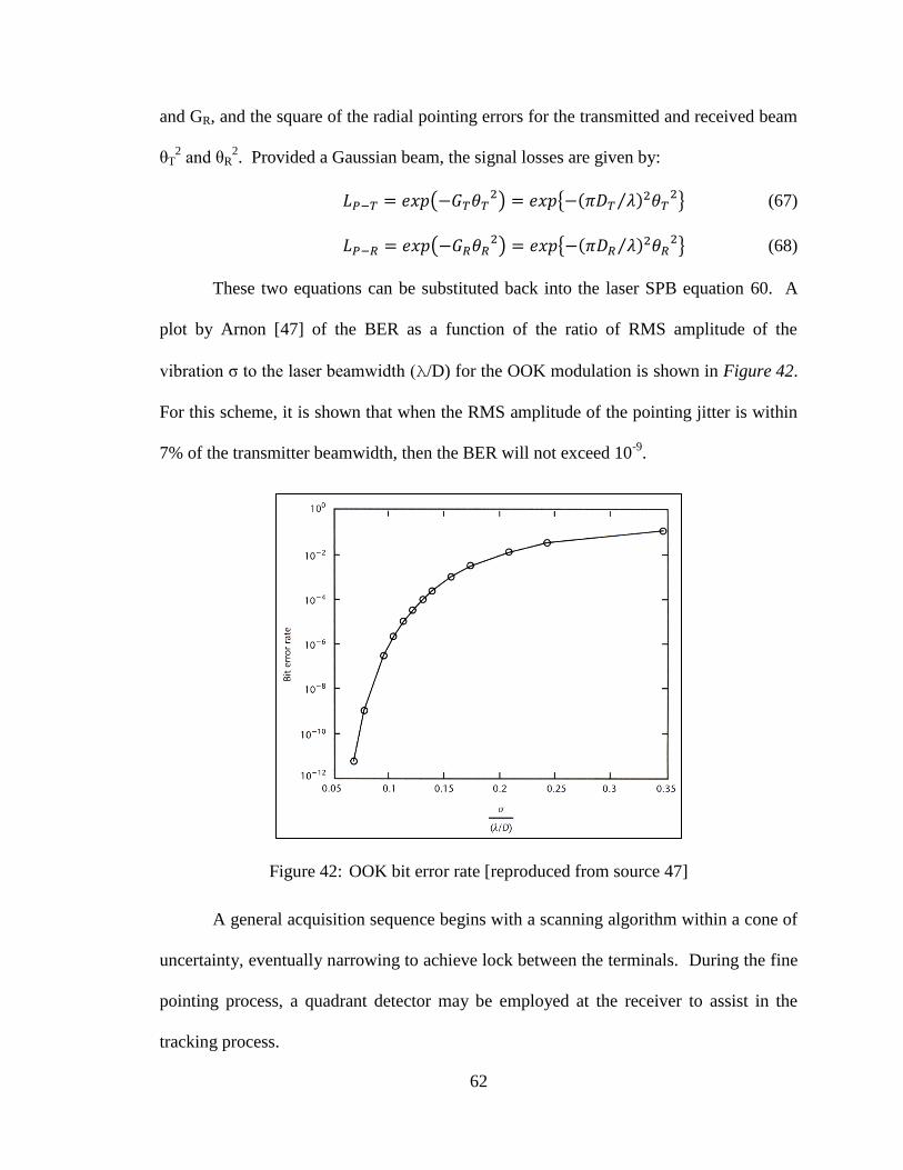
Figure 42: OOK bit error rate [reproduced from source 47] ...................................... 62
Figure 43: Cross-sectional stack-up of the power receiver ........................................ 64
Figure 44: Zalman heat pipe unit................................................................................ 65
Figure 45: Thermal analysis of the power receiver .................................................... 66
Figure 46: Two views of a complete HILPB receiver ................................................ 67
Figure 47: LIMO water-cooled turnkey laser diode system ....................................... 69
Figure 48: HILPB test facility at CSU ....................................................................... 70
Figure 49: Transmittance curve and coating on the protective fiber window ............ 71
Figure 50: Design and construction of the gimbaled yoke target mechanism ........... 72
Figure 51: Gimbal rig with receiver, power electronics and MUAV ......................... 72
Figure 52: Top level block diagram of the receiver electronics system ..................... 73
Page 20
xxiv
Figure 53: Flight ready power management and data handling system ..................... 74
Figure 54: DATAQ – functional block diagram ........................................................ 75
Figure 55: The data acquisition system GUI with example power curve .................. 75
Figure 56: Cell back-feeding with small overfill ....................................................... 77
Figure 57: Cell back-feeding with medium overfill ................................................... 77
Figure 58: Cell back-feeding with large overfill ........................................................ 77
Figure 59: Nine-cell square receiver .......................................................................... 79
Figure 60: Square receiver at 30% beam overfill, 23 W Pmp ..................................... 79
Figure 61: CAD layout of the radial orientation receiver design ............................... 80
Figure 62: Top cell I-V curve, 7.471 W Pmp .............................................................. 81
Figure 63: Right cell I-V curve, 7.467 W Pmp ............................................................ 81
Figure 64: Bottom cell I-V curve, 7.485 W Pmp ......................................................... 82
Figure 65: Left cell I-V curve, 7.385 W Pmp .............................................................. 82
Figure 66: Center cell I-V curve, 6.852 W Pmp .......................................................... 82
Figure 67: Four cell I-V curve, 19.976 W Pmp ........................................................... 83
Figure 68: Five cell I-V curve, 23.935 W Pmp ............................................................ 83
Figure 69: 48.09% illumination, 25.206 W Pmp at 26.2% Ƞ ...................................... 84
Figure 70: 37.72% illumination, 23.479 W Pmp at 31.12% Ƞ .................................... 85
Figure 71: 25.24% illumination, 22.488 W Pmp, at 44.39% Ƞ ................................... 85
Page 21
xxv
Figure 72: 9-cell radial array in the Northrop Grumman laser facility ...................... 86
Figure 73: Silicon spectral response ........................................................................... 87
Figure 74: Optical absorption for various semiconductor materials .......................... 89
Figure 75: Single VMJ cell laser power beaming test rig .......................................... 90
Figure 76: Wavelength maximum power I-V curves ................................................. 92
Figure 77: Wavelength input versus output................................................................ 93
Figure 78: Wavelength conversion efficiencies ......................................................... 93
Figure 79: Wavelength efficiency comparison ........................................................... 94
Figure 80: Wavelength output comparison ................................................................ 94
Figure 81: H and V profile cuts of the conditioned flat-top beam profile .................. 97
Figure 82: Mechanical illustration of the enclosed beam tube ................................... 97
Figure 83: Picture of the unenclosed beam homogenization optic stages .................. 98
Figure 84: Nine cell water cooled receiver illuminated with a flat-top beam ............ 99
Figure 85: Results of the flat-top beam with a 9-cell parallel array ........................... 99
Figure 86: Nine cell receiver illuminated with a Gaussian beam ............................. 100
Figure 87: Results of the Gaussian beam with a 9-cell parallel array ...................... 100
Figure 88: Peak power density test with a single VMJ cell ..................................... 101
Figure 89: Peak power density I-V curve with a single VMJ cell ............................ 101
Figure 90: LIMO laser system and diode module .................................................... 102
Page 22
xxvi
Figure 91: TEM00 model of the beam profile ........................................................... 103
Figure 92: Beam profiling setup ............................................................................... 104
Figure 93: Scanning to the extents of the beam profile ............................................ 105
Figure 94: Surface plot of the beam at 200 W of radiant power .............................. 106
Figure 95: Contour plot of the beam at 200 W of radiant power ............................. 106
Figure 96: 10th
order polynomial beam distribution ................................................. 107
Figure 97: Experiment setup for the off axis tests .................................................... 108
Figure 98: Progression of a horizontal axis rotation ................................................ 109
Figure 99: Progression of a vertical axis rotation ..................................................... 109
Figure 100: Horizontal and vertical off axis responses at 150 W radiant power ....... 110
Figure 101: Horizontal and vertical off axis responses at 200 W radiant power ....... 111
Figure 102: Horizontal and vertical off axis responses at 250 W radiant power ....... 111
Figure 103: Horizontal and vertical off axis responses at 300 W radiant power ....... 112
Figure 104: Horizontal and vertical off axis responses at 350 W radiant power ....... 112
Figure 105: Direct illumination at 350 W .................................................................. 113
Figure 106: Horizontal axis rotation of 45 degrees .................................................... 113
Figure 107: Vertical axis rotation of 45 degrees ........................................................ 113
Figure 108: Single (mono) crystalline photovoltaic cell ............................................ 114
Figure 109: 1 kHz clocking (top) of the laser diodes (bottom) .................................. 115
Page 23
xxvii
Figure 110: 10kHz clocking (top) of the laser diodes (bottom) ................................. 115
Figure 111: Mono-crystalline silicone photovoltaic cell output under 10 W
illumination exhibiting significant noise but good transient responsivity ...................... 116
Figure 112: Triple Junction TASC under pulsed illumination ................................... 117
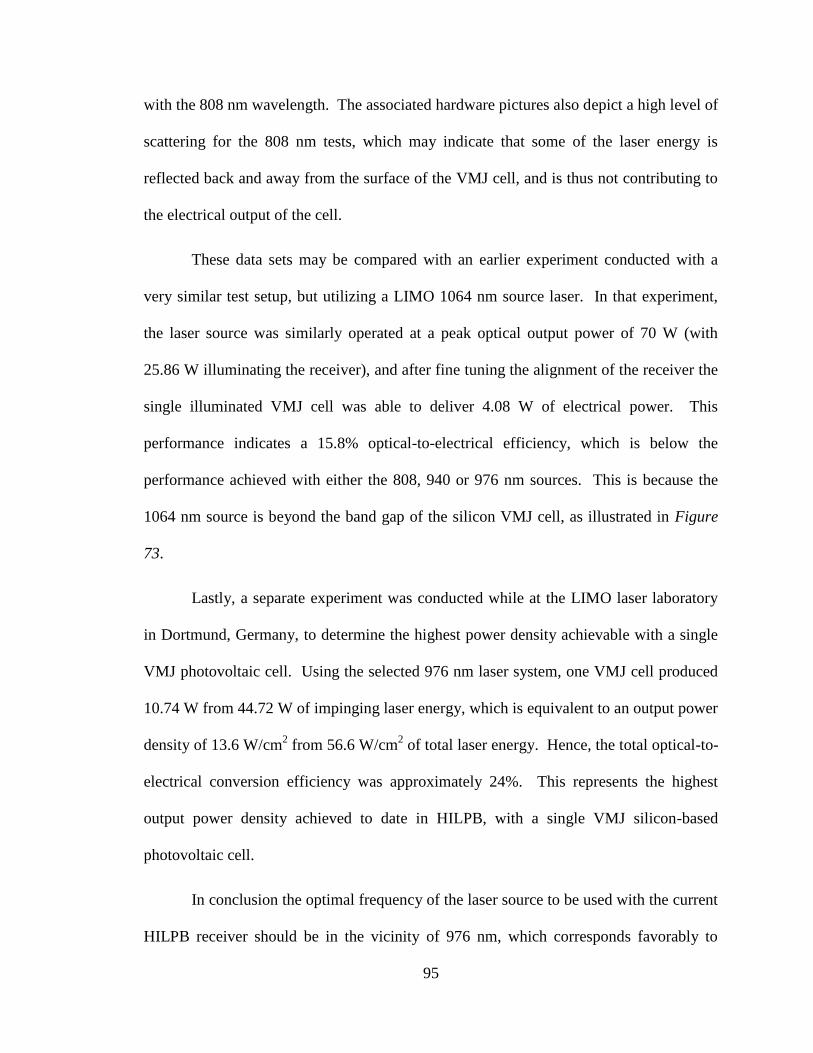
Figure 113: Triple junction photovoltaic cell output under 50 W illumination
exhibiting significant signal distortion............................................................................ 118
Figure 114: Quantum efficiency versus wavelength for a triple junction cell ........... 119
Figure 115: VMJ photovoltaic cell under pulsed illumination ................................... 119
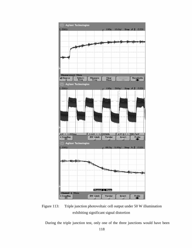
Figure 116: VMJ photovoltaic cell output under 30 W illumination ......................... 120
Figure 117: VMJ photovoltaic cell output under 75 W illumination ......................... 121
Figure 118: VMJ photovoltaic cell output under 120 W illumination ....................... 122
Figure 119: VMJ photovoltaic cell output under 165 W illumination ....................... 123
Figure 120: VMJ photovoltaic cell output under 210 W illumination ....................... 124
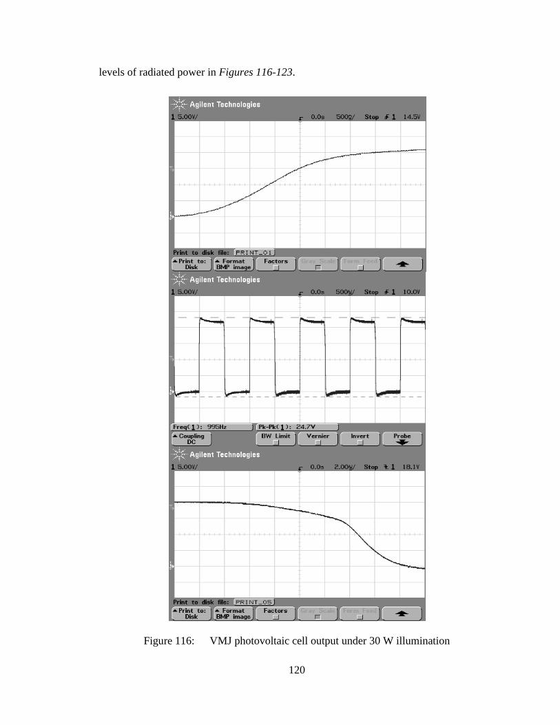
Figure 121: VMJ photovoltaic cell output under 255 W illumination ....................... 125
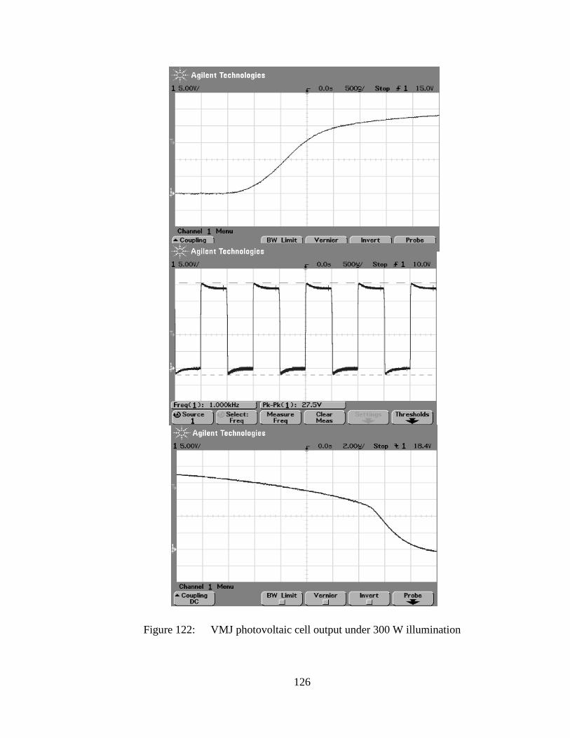
Figure 122: VMJ photovoltaic cell output under 300 W illumination ....................... 126
Figure 123: VMJ photovoltaic cell output under 345 W illumination ....................... 127
Figure 124: Discrete Fourier Transformation of the VMJ output .............................. 129
Figure 125: Optically-coupled switched-mode DC/DC power convertor abstraction for
the HILPB communications system................................................................................ 132
Page 24
xxviii
Figure 126: Clockwise from left: breadboard DC/DC convertor, data collection
electronics and active variable load ................................................................................ 133
Figure 127: Full duty cycle with 11.3327 W output .................................................. 134
Figure 128: Half duty cycle with 4.8078 W output .................................................... 135
Figure 129: Quarter duty cycle with 2.6789 W output ............................................... 135
Figure 130: Receiver output versus duty cycle .......................................................... 135
Figure 131: Source optics for the polarization experiment ........................................ 137
Figure 132: Rotating the linear source optic to characterize the dominant linear beam
polarization angle ............................................................................................................ 138
Figure 133: Introduction of the receiver optic for the polarization experiment ......... 139
Figure 134: Stage 1 (source) linear polarization rotation ........................................... 141
Figure 135: Stage 2 (receiver) linear polarization rotation ........................................ 141
Figure 136: Optical communications link budget ...................................................... 144
Figure 137: Modulating retro reflector ....................................................................... 146
Figure 138: Optical multi-function architecture schematic ........................................ 147
Figure 139: Potential integrated beamed energy representation ................................ 154
Page 25
1
CHAPTER I: INTRODUCTION
The heritage of optical communications extends back much farther than that of
RF technology, yet there is still a wide tradespace to explore in terms of exploiting the
capabilities offered in the optical domain. This chapter will highlight some of the major
advances in optical communication systems, and identify potential synergies with the
developed wireless power transmission system.
1.1 A Brief History of Free Space Optical Communications
The history of optical communications starts with using light for the
dissemination of news through what we could decipher with our own eyes, and over time
technology was developed to allow us to transmit and receive signals from increasing
distances. Some of the early incarnations included beacon fires, smoke signals, signal
markers and light houses. The achievable range was greatly increased through the use of
relay stations, such as with Chappe‟s optical telegraph system for the French military
during the early 1800‟s (Figure 1). Here, a series of mechanical lighted structures spaced
11 km apart could relay a message over 135 km in one minute, and reproduce 196
distinct symbols.
Page 26
2
Figure 1: Claude Chappe‟s optical telegraph
Later during the 1800‟s the optical telegraph system was widely adopted in both
the European and US railway systems in the form of semaphore signaling. In 1880,
Alexander Graham Bell patented what he referred to as his greatest invention, the
photophone (Figure 2). This system modulated human conversations onto visible light,
and demonstrated transmission across distances up to 200 m. This achievement may be
thought of as a very early predecessor to our modern fiber optic communications systems,
and legs of the system are still operational today.
Figure 2: Photophone transmitter and receiver set
Similar variations of the simple essence of these early forms of optical
Page 27
3
communication still exist today. The Navy has long used a signal lantern intermittently
covered with a shutter as a way to pass Morse code messages between vessels during
periods of radio silence [1]. Modern Air Traffic Control (ATC) towers still maintain a
multi-colored light gun as a backup device in case of radio failure, and all pilots are
versed in these procedures to accomplish safe queuing and landing in such an event. In
addition, the Federal Aviation Administration (FAA) employs a series of brightly colored
Fresnel lens instruments called Precision Approach Path Indicators (PAPI) which provide
a landing pilot visual feedback for the position of their aircraft relative to the optimal 3
degree glide slope [2]. These instruments are especially useful during night and carrier
operations where visual distortion is at its highest, and may be visible for several nautical
miles away depending on the atmospheric conditions.
Figure 3: Left: Naval signal lamp for transmitting Morse code, Right: PAPI indicating
glide slope of approaching aircraft
In the consumer electronics area, the first wireless remote control for television
was introduced by Zenith as the Flash Matic system in 1955 (Figure 4). This system
used four corner photocells to control the functionality of the set, and later evolved into
Page 28
4
the infrared remote control systems that are commonly used today.
Figure 4: Advertisement for the Zenith optical remote control
The advantages of high energy density and narrow beamwidth of the laser make it
a natural candidate for free space optical communication applications. These properties
allow for the propagation path of a laser communications link to extend farther than with
conventional lamps, favorably suggesting space-based communications applications.
After years of developing a direct detection system for the neodymium yttrium aluminum
garnet (Nd:YAG) laser operating at 1064 nm, the U. S. Air Force formalized an agenda to
develop and demonstrate a space-based laser crosslink in the early seventies. One of the
early stepping stones in developing the space-qualified laser communications hardware
for this directorate was the Airborne Flight Test System (AFTS), or the Air Force 405B
program, which was funded out of Wright Patterson Air Force Base (WPAFB) in Dayton,
Ohio. The 405B experiments consisted of an EC-135 test aircraft using a Nd:YAG laser
to prove the feasibility of transmitting information over a turbulent atmospheric channel
to a ground station. The program was successful in demonstrating up to 1 Gbps of
Page 29
5
optical data transfer rate, and achieved slant range distances to 100 km [3].
Following the success of the WPAFB 405B program, many investigations were
made into developing and refining the component technologies of the laser
communications system. Some of these advances were the emergence of avalanche
photodiode detectors, laser-diode pump sources, optical alignment techniques and
radiation hardening and optical coatings for system components. One notable
achievement made by the Massachusetts Institute of Technology‟s Lincoln Laboratory
(MITLL) was the development of a coherent optical communications system [4-6]. The
coherent system employed frequency shift keying (FSK) to modulate the transmitted
energy, and the receiver utilized a local oscillator laser source mixed with the received
signal to decode the message. Gallium-Arsenide photodiodes were used to detect the
energy, and data rates up to 220 Mbps were demonstrated in the lab.
In 1992, a breakthrough demonstration called the Galileo Optical Experiment
(GOPEX) demonstrated the ability to point ground-based lasers precisely to objects in
deep space, and to sense long-distance optical pulses. Both the Jet Propulsion
Laboratory‟s (JPL) Table Mountain Facility and the Starfire Optical Range (SOR) at
Kirtland Air Force base in Albuquerque, New Mexico were used to illuminate the charge
coupled device (CCD) camera on board the Galileo spacecraft at a range of six million
kilometers [7]. The optical pulses were successfully detected and then retransmitted back
to the ground for validation using the conventional spacecraft RF downlink.
A demonstrated study into atmospheric propagation effects has been made with
the European Semiconductor Laser Intersatellite Link Experiment (SILEX), in which one
link leg consisted of a 148 km horizontal terrestrial path along the sea between the
Page 30
6
Canary Islands [8]. The program utilized 0.79, 0.87, 1.064, 1.3 and 10.2 μm laser
wavelengths with up to 50 Mbps data rates, and measurements of absorption, scattering,
scintillations and turbulence were made. The signal strength and noise components from
the SILEX experiments across a 148 km terrestrial link are plotted simultaneously in
Figure 5, and it can be seen that the signal-to-noise ratio (SNR) when the sun is in the
field of view (FOV) of the receiver is approximately 25 dB, for the case when
atmospheric attenuation is at 4.5 dB.
Figure 5: SILEX signal strength and noise components [reproduced from source 8]
In a more recent measurement program conducted by the Lawrence Livermore
National Laboratory (LLNL), a 28 km laser link employing an adaptive optical system
was operated in Northern California [9]. Measurements of the wavefront distortion were
made at the receiver, and deformable mirror elements actuated by
Page 31
7
microelectromechanical systems (MEMS) corrected for the turbulence in the atmosphere.
This approach achieved a reduction in the bit-error-rate (BER) of the signal, and a data
rate of 20 Gbps was achieved.
In 2005, the Japan Aerospace Exploration Agency‟s (JAXA) Optical Intersatellite
Communications Engineering Test Satellite (OICETS) „KIRARI‟ in LEO and the
European Space Agency‟s (ESA) Advanced Relay and Technology Mission (ARTEMIS)
satellite in GEO successfully established an optical intersatellite communications link
[10]. Since then, the optical service has operated regularly and accumulated more than
1100 links totaling 230 hours to date, achieving 2 Mbps forward and 50 Mbps return
links.
Figure 6: ARTEMIS and OICETS optically linked
The maximum distance record for laser communications transmission was set in
2006 by NASA Goddard Space Flight Center‟s (GSFC) Geophysical and Astronomical
Observatory in Maryland, which successfully communicated with the Messenger
Page 32
8
spacecraft across a distance of approximately 25 million km [11]. Messenger was
outfitted with a Mercury Laser Altimeter (MLA), an instrument designed to map
Mercury's surface, and this was used to exchange laser pulses with the observatory to
demonstrate two-way deep space optical communication. The success of this technology
demonstration laid the groundwork for a proposed Mars Telecommunications Orbiter
(MTO) spacecraft to serve as a high speed optical data link for relaying scientific
information back to Earth from the other Mars orbiter and lander assets, but unfortunately
the program was cancelled due to funding problems [12].
In a more terrestrial accomplishment, within a few days of the World Trade
Center collapse in New York which severed many crucial fiber optic systems, high speed
communication services were reestablished to surrounding businesses clients through
deploying rooftop FSO systems from Lightpointe Communications, Inc. The systems
feature multi-Gb/s service across 1 km or better, depending on the atmospheric
conditions. The ability to quickly establish a backup network in an emergency situation
demonstrates the flexibility and rapid deployment capability of the FSO system, and its
ability to reduce downtime during periods of construction and repair.
Figure 7: FSO communications system deployed in an urban environment
Page 33
9
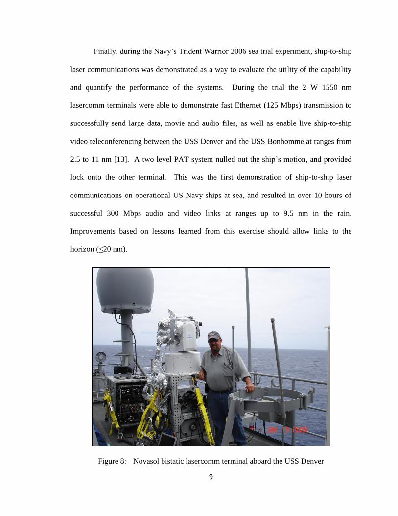
Finally, during the Navy‟s Trident Warrior 2006 sea trial experiment, ship-to-ship
laser communications was demonstrated as a way to evaluate the utility of the capability
and quantify the performance of the systems. During the trial the 2 W 1550 nm
lasercomm terminals were able to demonstrate fast Ethernet (125 Mbps) transmission to
successfully send large data, movie and audio files, as well as enable live ship-to-ship
video teleconferencing between the USS Denver and the USS Bonhomme at ranges from
2.5 to 11 nm [13]. A two level PAT system nulled out the ship‟s motion, and provided
lock onto the other terminal. This was the first demonstration of ship-to-ship laser
communications on operational US Navy ships at sea, and resulted in over 10 hours of
successful 300 Mbps audio and video links at ranges up to 9.5 nm in the rain.
Improvements based on lessons learned from this exercise should allow links to the
horizon (<20 nm).
Figure 8: Novasol bistatic lasercomm terminal aboard the USS Denver
Page 34
10
1.2 The HILPB System
A novel optical wireless power transmission system has been developed by a
cadre of researchers in the Industrial Space Systems Laboratory (ISSL) at Cleveland State
University (CSU) under contract (grant) from the Air Force Research Laboratory (AFRL)
Revolutionary Munitions Directorate at Eglin Air Force Base. This system utilizes
specially designed photovoltaic cells to receive and convert high radiant laser light into
electrical energy at appreciable efficiencies and substantial energy densities at the
receiver. The nominal optical-to-electrical conversion efficiency and output power
density at the cell level that has been achieved thus far are on the order of 44% and 20
W/cm2.
While typical photovoltaic devices may only handle broadband irradiances up to
100 mW/cm2, special photovoltaic cells developed by NASA John H. Glenn Research
Center (GRC) scientists at Lewis Field in the early 1990s, known as vertical multi-
junction (VMJ) cells, have demonstrated high conversion rates of 25% at up to 70 W/cm2
broadband solar irradiance. The primary application for the VMJ technology has been
for terrestrial solar concentration applications, such as the 1.5 kW integrated solar power
plants currently being deployed by Greenfield Solar Corporation [14].
Figure 9: Solar concentrator installation utilizing VMJ photovoltaic cells at NASA GRC
[reproduced from source 14]
Page 35
11
The silicon based VMJ cells differ fundamentally from conventional photovoltaic
devices, in that each individual chip contains multiple junctions of semiconductor
material, arranged to rest on its edge. This creates an edge-illuminated device, where the
electrical power may be easily routed through the low resistance junctions and delivered
on the outer edges of the cell. A typical 0.8 cm VMJ cell is constructed with 40 junctions
as shown in Figure 10, thus offering a nominal 24 V output, but this may easily be
tailored at the manufacturing stage to accommodate different bus voltages.
Figure 10: VMJ cell with attached silver ribbon electrical leads
The 25% optical-to-electrical efficiency figure for the VMJ cell is an average
value across all frequencies in the solar spectrum. The frequency dependent conversion
efficiency is the result of the silicon construction of the cell, and exhibits a peak at the
band gap (around 1.125-1.2 eV) of the silicon crystalline structure corresponding to the
near infrared region (IR-A) in Figure 11. It is this peak that may be exploited with
narrowband laser illumination, and it is expected that with further optimization, the
optical-to-electrical energy conversion efficiency of the cells may reach close to 60% for
incident laser light in the IR-A range.
Page 36
12
Figure 11: Spectral response plot for VMJ cell
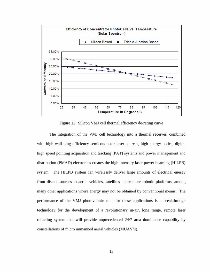
The VMJ cells are extremely robust and are able to withstand large thermal loads
because they are fabricated from high-grade silicon, and do not utilize the planar contacts
found in conventional solar cell topologies that trap heat under high irradiance levels. By
receiving the photonic energy through junction edges rather than on conventional wired
surfaces, the VMJ cell also maximizes the convertible photovoltaic surface area, and
eliminates exposing the contact wires to the high intensity light. As such, the cells are
able to operate continuously at high temperatures (with corresponding reduction in
efficiency-Figure 12) and are also able to survive and recover from exposure to
temperatures as high as 6000
C.
Page 37
13
Figure 12: Silicon VMJ cell thermal efficiency de-rating curve
The integration of the VMJ cell technology into a thermal receiver, combined
with high wall plug efficiency semiconductor laser sources, high energy optics, digital
high speed pointing acquisition and tracking (PAT) systems and power management and
distribution (PMAD) electronics creates the high intensity laser power beaming (HILPB)
system. The HILPB system can wirelessly deliver large amounts of electrical energy
from distant sources to aerial vehicles, satellites and remote robotic platforms, among
many other applications where energy may not be obtained by conventional means. The
performance of the VMJ photovoltaic cells for these applications is a breakthrough
technology for the development of a revolutionary in-air, long range, remote laser
refueling system that will provide unprecedented 24/7 area dominance capability by
constellations of micro unmanned aerial vehicles (MUAV‟s).
Page 38
14
Figure 13: Integrated HILPB system into an Air Force Pointer UAV
The ability to acquire and track a target, such as the UAV shown above, is a
critical system element to enabling the HILPB system. Synergies with the munitions
directorates may be identified, such as with the flagship megawatt class Airborne Laser
(ABL) research and development platform (Figure 14). Techniques such as on-line
sensing of the beam propagation through the atmosphere and adaptive optics have
successfully been employed to insure the integrity of the beam propagation and to reduce
jitter and compensate for air turbulence. The 600 km range of the ABL is a testament to
the maturity of the current HEL technologies, and these military successes can be
capitalized on with laser power beaming. The high-profile ABL program is an ongoing
effort, and new advances in laser control will be continually developed to increase the
range and accuracy of the beam.
Page 39
15
Figure 14: Boeing 747 ABL with laser turret [reproduced from source 15]
HEL laser tracking systems since the ABL have been progressively downsized,
resulting in a more portable source. The Navy laser weapons system (LaWS) is a ship
defense system currently under development. LaWS has been able to successfully
engage airborne targets in a marine environment, considering the atmospheric effects of
aerosols and dynamic platform motion. Such a system will see further downsizing and
tracking control capability in the future, realizing a more attractive deployable solution
for a HEL system.
Figure 15: Navy LaWS [reproduced from source 16]
Page 40
16
1.3 Future Potential for a High Intensity Laser Communications System
The current application for the Air Force HILPB program is to provide optical in-
air „refueling‟ of electric aircraft, which will allow indefinitely extended mission flight
times for 24/7 aerial domination. Beyond the immediate AFRL program, the HILPB
system can be used for many applications where power is needed but conventional
transmission lines are impracticality prohibitive. Examples may include deep space
exploration vehicles, reconfigurable power grids on the Moon and Mars, and establishing
ad-hoc emergency power to terrestrial areas in distress. By utilizing the VMJ cells as a
detector for communications, forward command and control information may be send
concurrently with the power transmission, resulting in a dual use system.
For example, the recent renewed interest in long duration, high altitude and
heavy-lift airship designs offers another opportunity for HILPB to extend mission
capability [17]. One of the primary applications for these proposed airships is to serve as
a stratospheric surveillance and communications relay platform that may be deployed for
a year at a time, and then be recovered for servicing and payload technology updating.
Among the propulsion sources considered for this application are electric motors, which
would operate off of onboard lithium-ion storage batteries and thin film photovoltaic
devices to supply the recharging energy. This type of platform may benefit from the
addition of a HILPB receiver to offset a portion of the photovoltaic array, which would
give it the ability to quickly recharge its power system from a remote location, or to
provide a transient enhanced capability.
Page 41
17
Figure 16: Airship optical link delivering power and/or communications
By incorporating a communications signal into the optical energy delivery path,
enormous amounts of data may be securely and covertly uplinked to the airship, and by
employing a modulated retro-reflector (MRR) on the airframe, comparable amounts of
data may be equally retrieved from the platform during the transmission [18]. Such a link
has been demonstrated by the Naval Research Laboratory (NRL) using a small UAV
helicopter as the flight platform to successfully return near-real time compressed video
information back to the interrogating ground station.
Figure 17: Data returned from UAV with a MRR to interrogating laser station
[reproduced from source 18]
Page 42
18
Beamed energy propulsion is a concept where directed energy is utilized to propel
a craft through a variety of means such as a thermal engine, or by generation of a plasma-
induced detonation wave (Figure 18). These types of beamed energy vehicles are being
developed as a low cost alternative way to achieve hypersonic velocities in the
atmosphere, and to launch payloads to orbit. The beam riding properties of the lightcraft
under conditions of intense directed illumination lend themselves favorably to utilizing
high energy photovoltaic devices that could enable both energy harvesting and
communications capability to the craft.
Figure 18: Flight model of the laser boosted lightcraft [reproduced from source 19]
In each of these scenarios, the ability to integrate communications capability with
wireless power transmission offers a high value added technology with a minimal amount
of modification to the existing system infrastructure. Uplinks, downlinks and crosslinks
to a satellite backbone system could be augmented with HILPB to develop a virtual
power and communications grid network that could deliver both information and power
Page 43
19
anywhere in the world and beyond. The performance metrics of such a system will be
discussed in the following chapters, along with design recommendations and avenues for
future research.
1.4 Document Organization
A literature review of optical communications systems including comparisons
with RF based systems, performance metrics, system trades and design parameters
appears in Chapter 2. The experimental setup and research methodology is described in
Chapter 3, and the experiments conducted and data analysis appears in Chapter 4.
Finally, the results and conclusions are stated in Chapter 5, with recommendation for
future work in Chapter 6.
Page 44
20
CHAPTER II: LITERATURE REVIEW OF LASER COMMUNICATIONS
2.1 Advantages of Optical Communications
As early as the first successful implementation of Light Amplification by
Stimulated Emission of Radiation, or LASER, in 1960, optical communications has been
one of the principal considered applications for the technology [20]. Lasers lend
themselves favorably to the field of communications because of several unique
characteristics inherent in the technology. The extreme directivity of the transmitted
photonic energy in the optical regime, when compared to that of conventional microwave
technology, results in several systems level benefits. The directionality of a beam
exhibiting a Gaussian energy profile is described by the angle of beam divergence θ,
subject to the diffraction limit, and as a function of the wavelength of the beam λlaser and
the diameter of the beam waist (Dlaser) at the aperture of the transmitting telescope. [21]
(1)
As an example, for a 1.0 micron laser with an aperture diameter Dlaser=10 cm the
resulting the beamwidth would be 22.4 μrad. Expression 1 may also be used to
approximate the directionality of a pattern transmitted from a microwave antenna with a
Page 45
21
diameter Dmicrowave and radiating at a wavelength of λmicrowave. By comparing both of
these calculations, the first benefit of laser optical communications is revealed. For the
X-band antenna dish onboard the workhorse Defense Satellite Communications System
(DSCS-2) satellite the resulting beamwidth would be 3° [22]. At the point of ground
intercept on the Earth‟s surface at the equator from a geosynchronous orbit
(approximately 35,786 km (22,236 mi) above mean sea level altitude at the equator), the
example laser beam would illuminate a circular area 800 m in diameter, while the
microwave footprint would encompass a diameter of 1,880 km as illustrated in Figure 19.
This is a best case scenario comparison of the two technologies, in the sense that as the
selected ground intercept area moves away from the equator longitudinally the circle of
illumination will elongate into an ellipse, and the ratio between the two intercept areas
will change. The difference in footprints will have privacy implications with securing a
monitored intercept area on the ground, and as previously shown in Equation 1 this is
wavelength driven.
Figure 19: Optical vs. RF ground intercept area [reproduced from source 23]
Page 46
22
With the comparably short optical wavelengths, high directivity may be achieved
even through relatively small apertures. This is demonstrated by:
(2)
The antenna/aperture directivity ratio may be expressed as:
(3)
In the aforementioned example for λlaser=1.0 micron with aperture Dlaser=10 cm
and beamwidth θlaser=22.4 μrad, the resulting antenna/aperture gain Glaser=104 dB. To
achieve that same amount of gain utilizing X-band RF (λmicrowave=3 cm) the antenna
surface would have to be 3 km across. Clearly this is a prohibitive size for operation in
space, even for lightweight deployable and inflatable apertures. In a general sense on the
receiving side, the microwave antenna needs to be much larger than the optical aperture
in order to appreciably encompass the transmitted energy. This creates a fundamental
constraint on the physical architecture of an RF based system design.
The narrow beamwidth of the optical system does impart a challenge to the
pointing, acquisition and tracking (PAT) system across long distances. By utilizing other
technologies such as GPS satellites, star trackers and inertial guidance instruments to
obtain attitude and position information, the acquisition process may be accomplished in
a timely manner. In addition a beacon may also be used to aid in the acquisition process,
in a similar manner to RF communications. Table I depicts a scenario in which a GEO
satellite accomplishes acquisition and closes the link with a LEO satellite to begin the
communications transmission within 7.5 seconds.
Page 47
23
TABLE I: GEO to LEO acquisition time sequence [reproduced from source 23]
Considering privacy comparisons between the interception of laser and
microwave footprints, Figure 20 shows a contrast of the relative received power with
respect to perpendicular distance from the beam‟s central axis. In the case of a 1 arcsec
(290 µrad) beamwidth laser, at 0.4 miles from the central axis the power is 40 dB down
from the peak at the aperture. With the 35 GHz microwave signal at ¼° beamwidth, the -
40 dB point would not occur until approximately 100 miles from the center of the beam.
This indicates a substantial loss of privacy in the microwave case.
Page 48
24
Figure 20: Laser and microwave privacy comparison [reproduced from source 23]
When comparing the atmospheric propagation implications of optical versus RF
bands electromagnetic radiation, it can be seen in Figure 21 that transmittance windows
exist across both spectral regions. Within the microwave RF regime the opacity is
relatively constant, while the optical bands vary greatly depending on wavelength. This
variability places a constraint on the design of an optical system, in that the frequency
must be carefully selected to optimize the overall system capability. At 1550 nm,
substantial investment has been made by the telecommunications industry to advance the
development of supporting components for fiber optic systems, and a significant
transmission window through the earth‟s atmosphere at this frequency also exists.
Page 49
25
Figure 21: Atmospheric opacity across the electromagnetic spectrum [reproduced from
source 24]
Another advantage that laser optical communications has over conventional RF is
the enormous amount of information carrying potential in the Terahertz carrier beam.
For example, a mode locked laser operating near 1 µm (2.86 x 10¹⁴
Hz) and producing 30
ps repetition rate pulses will have a bandwidth of at least 30 GHz. It is important to note
that the high rate of repetition is necessary to achieve the information bandwidth, and this
may be challenging to accomplish with current single laser implementations. One way to
achieve high repetition rates is to employ a system similar to that of a Gatlin gun, where
multiple laser sources, each producing picosecond pulses (offset from each other), are fed
Page 50
26
into a common aperture. This technique relaxes the pulse repetition requirement on any
one laser, and may be used to accomplish an information bandwidth of 30 GHz. In that
case, the bandwidth-to-frequency ratio would be:
(4)
In this example the optical carrier could accommodate 1,000 channels that are
each 30 GHz wide at a carrier capacity of 10% as given by:
(5)
This amount of bandwidth can be used to carry an enormous amount of
information, but the usefulness of this bandwidth will be limited by factors such as the
ease with which information can be imposed upon the beam, the ability for the channel to
support it and the capability of the receiver to detect and decode it. These factors will be
described in subsequent sections on modulation and demodulation techniques and
channel effects.
Finally, in comparing the future growth potential of RF versus optical systems, it
is important to note the diminishing available spectrum allocation for certification and
licensing in the RF domain from the International Telecommunications Union (ITU) and
the National Telecommunications and Information Administration (NTIA), while the
entire optical region still remains unregulated and free of license fees, beyond nominal
hazard zone restrictions. This currently frees optical technology from the frequency
allocation issues and interference problems encountered with RF counterparts.
Page 51
27
2.2 Beam Polarization
Before venturing into modulation and detection techniques, a discussion first must
be made into the polarization of light since this may serve as a unique optical tool to aid
in modulation process. At a given point in space and instant in time the electric-field of a
light wave points to a particular direction, and is described by a vector ε. This electric-
field lies in the x-y plane, and the vector is perpendicular to both the direction of travel of
the wave and the instantaneous direction of the magnetic-field of the wave. The direction
of the electric field-vector is described as the direction of polarization of light, and since
lasers produce light with highly oriented electric-fields, it follows that a degree and form
of polarization will also exist. Given a plane wave of frequency ν and an angular
frequency , and travelling in the z direction with a velocity c, the electric-field may
be represented as:
(6)
Where the complex envelope A has components Ax and Ay:
(7)
By tracing the endpoint of the vector at each position z as a function of
time t, the direction and type of polarization may be described. For example, the
complex components can be represented in terms of their magnitude and phase, given by:
(8)
(9)
Substituting into the electric-field equations obtains:
(10)
Page 52
28
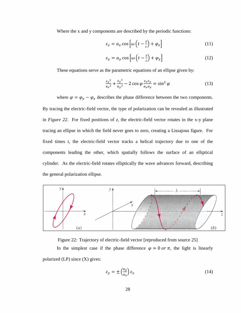
Where the x and y components are described by the periodic functions:
(11)
(12)
These equations serve as the parametric equations of an ellipse given by:
(13)
where describes the phase difference between the two components.
By tracing the electric-field vector, the type of polarization can be revealed as illustrated
in Figure 22. For fixed positions of z, the electric-field vector rotates in the x-y plane
tracing an ellipse in which the field never goes to zero, creating a Lissajous figure. For
fixed times t, the electric-field vector tracks a helical trajectory due to one of the
components leading the other, which spatially follows the surface of an elliptical
cylinder. As the electric-field rotates elliptically the wave advances forward, describing
the general polarization ellipse.
Figure 22: Trajectory of electric-field vector [reproduced from source 25]
In the simplest case if the phase difference , the light is linearly
polarized (LP) since (X) gives:
(14)
Page 53
29
Which describes a straight line of slope , where the + and – signs
correspond to . Here the polarization is planar, and the electric-field oscillates
in the direction of the slope as illustrated in Figure 23.
Figure 23: Linear polarization [reproduced from source 25]
If the phase difference , and the components are equivalent in
magnitude where , then the electric-field components can be written:
(15)
(16)
From which:
(17)
…describing the equation of a circle, due to the equivalent component
magnitudes. When , at a fixed position z the electric-field rotates in a
clockwise direction and this case is called right circular polarized (RCP). Conversely
when , at a fixed position z the electric-field rotates in a counter-clockwise
direction and this case is called left circular polarized (LCP), as illustrated in Figures 24a
and 24b.
Page 54
30
Figure 24: Circular polarization [reproduced from source 26]
There are several ways to manipulate the polarization of light. One of the most
familiar methods is through polarization by absorption, which is generally how
polarization is achieved in sunglasses for eye protection. Such an optical material
consists of elongated molecules oriented in a similar grid direction, which provides a path
for electrons to move. When an electromagnetic wave of random polarization passes
through the material, the electric field components that are aligned parallel to the material
grid will be absorbed and reflected. The resulting transmitted light will be LP at an axis
perpendicular to the molecular grid as shown in Figure 25, and will consist of roughly
one-half of the original light, minus any transmission losses in the optics. This axis is
called the polarizer axis.
Page 55
31
Figure 25: Grid polarizer [reproduced from source 26]
In the case that the impinging light is already linearly polarized, the amount of
transmitted light is dependent on the angle θ between the electric field vector of the
original light wave and the polarizer axis. The Law of Malus describes the resulting
irradiance function as:
(18)
as illustrated below in Figure 26. At , I0 is at its maximum transmitted
irradiance.
Figure 26: The law of Malus [reproduced from source 26]
Page 56
32
In polarization by reflection, the interaction of the light wave with the surface of a
material will allow for a manipulation of the beam. In this case the light component with
a polarization vector parallel to the surface face is preferentially reflected, while the
remaining light is refracted due to the refractive indices at a critical angle. The key is to
obtain an angle that allows for the maximum amount of transmission, while reflecting out
the undesired polarization components. This angle is referred to as the Brewster angle, as
given by:
(19)
where n1 and n2 are the refractive indices of the two respective transmission
mediums. Brewster‟s Law is illustrated using several stages in Figure 27. In this
example, a series of optical stages are used to separate the s-polarized (light polarized
perpendicular to the plane of incidence) and p-polarized (light polarized in the plane of
incidence) components of the light. For a Brewster angle where no p-polarized light is
reflected, only a portion of the s-polarized light is depleted. Hence, it is necessary to use
multiple optical stages in order to avoid reducing the p-polarized light while
simultaneously removing the s-polarized light.
Figure 27: Series Brewster angle plates [reproduced from source 26]
Page 57
33
Another way to manipulate the beam polarization is with birefringent crystals.
Within the crystal there are two perpendicular axes known as the fast axis and the slow
axis. The difference in these axes means that light with different polarizations will travel
through the crystal at different refractive indicies. Light with polarization parallel to the
fast axis will travel though the crystal faster than light with polarization parallel to the
slow axis. Such a crystal can be used as a retarder to a polarization component, and this
allows for a manipulation of the overall wave polarization as illustrated in Figure 28.
When used in this fashion the birefringent crystal is referred to as a wave plate.
Figure 28: Example of a half-wave plate [reproduced from source 27]
The amount of relative phase shift Γ imparted on the polarization is dependent on
the birefringence Δn and the length of the crystal L as given by:
(20)
The above example illustrates a half-wave plate, resulting in a transmitted wave
Page 58
34
that is orthogonal to the orthogonal polarization. Additionally, a quarter-wave plate
creates a quarter wavelength phase shift, and this can be used to change linearly polarized
light into circularly polarized light and vice-versa.
Figure 29: Birefringent wave plate [reproduced from source 27]
Extending the birefringent crystal further, the index of refraction of the fast axis
nfast is not equal to the index of refraction of the slow axis nslow. Therefore a beam of
light incident on the crystal may be partitioned into two component polarization waves
through selective refraction. By cutting the crystal at an oblique angle as shown in
Figure 30, the two linearly polarized rays leave the prism at separate diverging angles.
Such a device functions as a polarizing beam splitter, and is known as a Wollaston prism.
The device consists of two triangular Calcite prisms cemented together with orthogonal
crystal axes.
Figure 30: Illustration of a Wollaston prism [reproduced from source 26]
Page 59
35
There are many other methods for manipulating the polarization of the beam. The
output of many laser systems is predominantly linearly polarized, with a high degree
exceeding 1000:1 between the light polarized in one direction and the orthogonal
component. This is due to factors such as Brewster surfaces that may be employed
within the laser construction for efficiency, or birefringence associated with the optical
components. These techniques may be employed to further condition the beam for
communications purposes through optical multiplexing, as will be discussed in the next
section.
2.3 Modulation and Demodulation Techniques
The process of imposing an information signal on a laser beam carrier is known as
modulation, and this is achieved with a device called a modulator. Modulators may vary
in complexity from simple external electromechanical shutters to solid state electro-optic
(EO) devices positioned within the laser cavity. In total, there are five characteristics of a
laser beam that may be altered for the purpose of sending a message: power, frequency,
phase, polarization and direction. In practice, phase and direction modulation are seldom
used due to system complexity.
The detection process in an optical communication system is required to convert
the variations in received light to variations in signal voltage, in order to decode the
message. Historically, laser detectors have been divided into either thermal or quantum
detectors. Although thermal detectors cover a wide range of wavelengths due to their
response of the total absorbed energy, they are neither as fast nor as sensitive as quantum
detectors, such as with photomultiplier tubes and semiconductor photodiodes.
Page 60
36
Photomultiplier tubes are an appropriate detector in cases of low light levels and high
bandwidths, but they are generally bulky, not especially rugged, and require supply
voltages from hundreds to thousands of volts. Photodiodes also have a rapid response
time, but are generally limited to maximum radiant power levels of 1 to 100 mW, beyond
which permanent thermal damage may occur [28]. In addition, they also require a power
supply to operate, although the voltages are far lower than that of the photomultiplier
tube. The VMJ photovoltaic cells employed in HILPB share the same charge carrier
properties of the photodiode lending to high sensitivity, but they additionally offer
continuous operation under intense illumination, and do not require external biasing.
2.3.1 Direct Detection Receiver
The nature of the detection operation at the receiver is determined by the type of
modulation scheme chosen at the source. Whenever the message information is
contained through variations in the irradiance of the light, a direct detection scheme is
used at the receiver. Direct detection provides electrical variations proportional to the
light variations, and these signals can be processed by appropriate demodulation
algorithms. The direct detection receiver offers design simplicity, uses few components
and does not depend on the phase of the signal. Its main function is to identify when
more than a few photons have been collected per bit, indicating a binary 1. When fewer
photons are received, a 0 is indicated. By minimizing background noise, the
differentiation between a 0 and a 1 can be made more successfully. The signal-to-noise
ratio (SNR) for a direct detection receiver can be calculated by starting with the ratio of
optical power received PC to the energy per photon hν, resulting in the collected number
Page 61
37
of photons per second:
(21)
Considering charge q, and the quantum efficiency of the receiver Q (ratio of
output photoelectron rate to input photon rate), the signal current may be represented by:
(22)
By feeding the signal into a load resistor RL and considering the photoelectric
current gain G, the signal power Ps is expressed through:
(23)
The noise components at the receiver will consist of the shot noise (due to the
signal current iSS, the background current iBS and the dark current iD) and the thermal
noise inT. The total squared noise current is given by the following summation of
components:
(24)
Where the components are defined as:
(signal current) (25)
(background current) (26)
(dark current) (27)
(thermal noise current) (28)
Bn = noise bandwidth
NO = electronic thermal noise spectral density (watts/Hz)
The previous equation is multiplied by the load resistance, and divided into the
signal power to form the SNR ratio:
(30)
Page 62
38
The simplicity of the architecture of the direct detection receiver can be seen in
Figure 31. The primary reason for this simplicity is that the receiver is designed to
collect photons without any respect for the signal phase.
Figure 31: System block diagram for a direct detection laser receiver
On-off key (OOK) modulation of the laser beam is one of the most commonly
employed schemes with direct detection communications [29]. OOK is a simplification
of the amplitude shift keying (ASK) method, in that the source transmits a large
amplitude carrier when it wants to send a binary value of '1', and no carrier when it wants
to send a '0'. As illustrated in Figure 32a, a typical OOK waveform is shown
representing the binary string „10110‟. A modification to this scheme would be pulse
polarization binary modulation (PPBM) which may incorporate two orthogonal
polarization states for the laser beam to represent a binary value of 1 or 0, as shown in
Figure 32b. For example, these two polarization states could be horizontal and vertical
linear, or left and right circular, and this would offer an improved average received
laser oscillator
tracking
beam pointing
optical antenna
laser modulator
Data Transfer Link Model
data modulator
G
channel
(photons) Pc
(signal + background)
background noise (solar, stars, lunar & Earth shine)
photo detector
data demodulator
data decoder
optical antenna
data encoder
optical filter
P P E
current multiplication
(shot and preamp noise)
electronic filter
load
(thermal noise)RL
Page 63
39
energy for the HILPB case, along with allowing easy detection for loss of signal, since
the receiver is expecting a pulse at each time interval. PPBM also has the advantage of
operating in a noisy environment without substantially increasing the BER, when
compared with other modulation schemes. The implementation of a PPBM system
requires a dual channel polarized receiver.
Figure 32: OOK and PPBM waveforms
Pulse-gated binary modulation (PGBM) is a one-bit-per-pulse stream that is well
suited for a mode-locked laser with a high speed EO modulator, and when used in
conjunction with a pulse-gated receiver the system achieves high noise discrimination.
An illustration of the individual wave components that construct a PGBM system are
shown in Figure 33.
Page 64
40
Figure 33: Pulse-gated binary modulation waveform progression
Given a number of signal and background (noise) photoelectrons and extinction
ratio E (ratio between number of received signal photoelectrons during a desired pulse to
the total number of photoelectrons when no pulse is desired), an expression for the
probability of error is given:
(31)
Where the components are defined as:
p = probability of transmitting a pulse
(1- p) = probability of not transmitting a pulse
Pnd = probability of no detection for a transmitted pulse
Pfd = probability of false detection for no pulse
The signal and noise follow a Poisson distribution, and the probability of a false
detection of no pulse is described by [30]:
(32)
Where the components are defined as:
Page 65
41
T = optimum threshold (maximum likelihood ratio detection)
= mean number of signal photoelectrons per decision period
= mean number of background (noise) photoelectrons per period
Likewise the expression for the probability of no detection of a transmitted pulse
is described by:
(33)
The probability of a false detection by the receiver for a finite extinction ratio E
is:
(34)
For the PGBM modulation scheme, the error rates are plotted for different
numbers of photoelectrons with a constant extinction ratio E= 100 in Figure 34. The
average number of signal photoelectrons ranges from 0 to 100, and the resulting BER
ranges from near 1.0 to 10-8
. These values will be used later to demonstrate a laser signal
power budget.
Figure 34: BEP plot for PGBM [reproduced from source 30]
Page 66
42
2.3.2 Coherent Detection Receiver
Although many optical communications systems employ direct detection, it is
also possible for variations in the phase or frequency of the laser field to contain the
message information. A coherent detection method is used in these cases to measure the
variations using superposition, by comparing them with the stable phase or frequency
from a local coherent reference field using interferometric techniques as shown in
Figure 35. In this arrangement, the detector receives the signal-bearing laser beam
combined with energy from a local oscillator source, and the resulting interference
between the two fields will contain information about both the amplitude and the phase of
the signal. The coherent optical reception method is analogous to the superheterodyne
radio receiver, and likewise it offers a reduction of the accumulated noise effects.
Figure 35: Diagram of a coherent optical communication receiver system
laser oscillator
tracking
beam pointing
optical antenna
laser modulator
Data Transfer Link Model
data modulator
G
channel
(photons) Pc
(signal + background)
background noise (solar, stars, lunar & Earth shine)
photo detector
data demodulator
data decoder
optical antenna
data encoder
optical filter
P Pfo-fc
IF amp
(shot and preamp noise)
IF filter
load (thermal noise)
RL
beam combiner
local laser oscillator
local oscillator controller
Page 67
43
Considering ωS as the optical carrier frequency (on the order of 1013
to 1015
depending on the laser source) and the signal bearing modulation φ(t), then the electric
field of the incident signal waves can be described by:
(35)
In the case of frequency modulation dφ/dt is proportional to the message signal,
and in the case of phase modulation φ(t) is proportional to the message signal.
Considering ωR as the local oscillator frequency at the receiver (not necessarily the same
as ωS), then the electric field of the local oscillator can be described by:
(36)
By superposition, the composite of these two waves arriving at the detector can be
described by the total wave field:
(37)
The two optical frequencies, ωS and , ωR are much too high to be sensed by the
detector. Instead, the detector generates a voltage proportional to the total photon flux,
which is the time average of the square of the electric field. This expression is essentially
the mixer output and is proportional to:
(38)
In this expression, , and this difference can be chosen to be well
within the response performance of the detector. In the case , the local oscillator
equals the carrier frequency and the operation is described as homodyne detection. If
, then the local oscillator is different than the carrier frequency and the operation
is described as heterodyne detection. The output signal is converted back into the
original message information using conventional phase or frequency demodulation
Page 68
44
techniques, depending on which method was used at the transmitter.
In general, the coherent optical detection method has some critical issues
concerning practical implementation. The heterodyne receiver requires a high surface
quality optical coupler that can precisely align the mixed signals to prevent distortion of
the interference term. Many laser oscillators do not exhibit the necessary frequency
stability to make the communications scheme successful. Laser light, although
narrowband, is not truly monochromatic and thus small variations in would not be
able to be distinguished from in practice unless some degree of signal degradation
can be accepted. At the time of this writing frequency tunable lasers generally do not
approach the average power levels typically encountered with HILPB. In addition,
induced phase distortion in the received optical signal will introduce a higher BER when
compared with a direct detection scheme. Finally, the added system complexity of a
coherent system will limit its potential application to larger platforms.
2.4 Terrestrial and In-Space Issues
Clearly directionality and bandwidth are two inherent advantages of a laser based
communication system, but there are also a few unique challenges when considering the
channel. The optical path may be disturbed by turbulent atmospheric conditions, and rain
or fog may create significant signal attenuation. Additionally, a link across a
considerable distance such as one established in space will experience an appreciable
range loss.
Page 69
45
2.4.1 Terrestrial Links
Long range transmission of a laser signal beam through the atmosphere offers an
array of challenges. For a terrestrial communication link there are a number of
components that can cause signal loss such as absorption and scattering by airborne
molecules and aerosols. Wavefront distortion by atmospheric turbulence resulting from
variations of the index of refraction along the beam‟s path can create problems for
successful demodulation at the receiver, especially in the case of coherent detection. An
understanding of these channel effects may be used to correct such distortions with tools
such as an adaptive optics system (AOS), and this warrants a venture into describing the
phenomena.
The atmospheric turbulence parameters may be calculated by first starting with
the Hufnagle-Valley-Bufton model [31] for the atmospheric index of refraction structure
parameter across the range of visible frequencies:
(39)
Where the components are defined as:
h = altitude in meters
W = RMS windspeed in m/sec
A = nominal value of CN2(0) at the ground in m
-2/3
(approximately 1.7×10⁻⁴ m-2/3 during daytime and 8.4×10⁻¹⁵ m-2/3 at
Page 70
46
night)
In general, CN2 varies from 10
-13 m
-2/3 for strong turbulence to 10
-17 m
-2/3 for weak
turbulence, with 10-15
m-2/3
often defined as a typical average value [32]. The 0th
turbulence moment μO, for a 0° zenith angle is evaluated from:
(40)
The coherence diameter r0 is obtained from:
(41)
The turbulence signal coupling efficiency ΓT is given by:
(42)
The need for an AOS is determined from the expression for ΓT. If the ratio of
D/p0<<1, this indicates little distortion and thus does not require an AOS. Conversely, in
instances when D> p0, an AOS should be employed. In this case, the SPB should be
multiplied by the ΓT factor in order to remain an effective measure of photoelectrons per
bit during turbulent atmospheric conditions.
The basic attenuation constant for beam propagation through the atmosphere is
made up of the molecular and aerosol scatter and absorption constants as given by:
(43)
Where the components are defined as:
αM = molecular absorption constant
βM = molecular scattering constant
αA = aerosol absorption constant
βA = aerosol absorption constant
The attenuation is expressed using Beer‟s Law with:
Page 71
47
(44)
Where the components are defined as:
TR = transmittance
I0 = initial beam intensity
IZ = beam intensity at distance z from the aperture
The total molecular absorption constant αM is computed by summing over each of
the prevalent absorber components, such as H2O and CO2, when the wavelength of the
beam is greater than the size of the molecules.
The molecular scattering constant is derived from a harmonic field inducing a
dipole as discussed by Hugo Weichel [33], and it is described as the Rayleigh Scattering:
(45)
Where the components are defined as:
f‟ = effective number of electrons per molecule that oscillate at the natural
frequency ω0
e = charge of an electron
λ = wavelength of the laser beam
λ 0 = wavelength related to ω0
When the laser beam wavelength is similar to the size of the particles, and
interaction of Mie Scattering with small water droplets and aerosols occurs [34]. The
fractional decrease in laser intensity when passing through an elementary volume is given
by
(46)
Where the components are defined as:
Page 72
48
I = laser intensity
A = cross sectional area of element
dz = length of element
a2dz = volume of element
NAdzπa2 = total cross section of the particles
N = total number of particles in the elementary volume interacting with
the laser beam
K = attenuation factor from scattering and absorption of similarly-sized
particles as λ
By substitution, equation 46 may be rewritten as:
(47)
Where the components are defined as:
Nσ(a,λ)dz = Mie attenuation coefficient
σ = Kπa2 = Mie attenuation cross-section
Many empirical measurements of aerosol scattering coefficients as a function of
laser wavelength have been made across the world. Hugo Weichel [33] related the
scattering coefficient to both Mie and Rayleigh scattering by:
(48)
In this relation, the C1, C2 and δ constants are determined by the aerosol density
and the size distribution of the particle sizes. The second term may be effectively
neglected for most wavelengths exceeding the UV region.
The transmittance may be calculated by knowing the visible range and the relative
humidity. An example plot for the coefficient of extinction is shown in Figure 36 for a
Page 73
49
23 km visibility. In this example it can be seen that at 1.0 μm, the total aerosol extinction
is about 10-1
/km.
Figure 36: Aerosol absorption extinction [reproduced from source 33]
When calculating the beam propagation through weather particulates whose
physical size is beyond that of the laser wavelength, such as with haze, fog and rain, there
is a negligible dependency on wavelength and the scattering coefficient may be expressed
as:
(49)
Where the components are defined as:
Δx/Δt = rate of rainfall in centimeters of depth/sec
a = raindrop size in centimeters
An example with raindrop radii between 0.025 and 0.325-cm and a laser path-
length of 1.8-km is shown in Table II, with a transmittance ranging from 0.88 to 0.38
depending on the intensity of the rainfall.
Page 74
50
TABLE II: Laser transmittance through rainfall [reproduced from source 34]
For a similar cloudburst condition yielding a rainfall rate of 10-cm/hour, a range
of scattering coefficients as a function of drop radii and concentration of drops per square
cm are tabulated in Table III. These values may be used in the Beer‟s Law expression to
estimate the signal attenuation.
TABLE III: Cloudburst Scattering Coefficients [reproduced from source 35]
Page 75
51
Table IV is a collection of experimental measurements of signal attenuation due to
absorption and scattering in a range of environments, from clear weather to snow at
distances from 1- to 100-km [36, 37]. Extending the table, a 0.53 μm laser beam
penetrating a cumulus cloud containing a liquid water concentration of 1.77 gm/m3 and a
thickness of 230-m will produce an attenuation of 17-dB. At a thickness of 677-m the
attenuation becomes 50-dB, and at 2,100-m the attenuation becomes 156-dB [36]. These
losses were calculated from a number of software tools developed by the Air Force
Geological laboratory (AFGL), and can be used to determine repeater station placement
and give a measure for BER.
TABLE IV: Weather parameter attenuation [reproduced from source 36, 37]
Page 76
52
The Air Force Research Laboratory (AFRL) Space Vehicle Directorate, in
collaboration with Spectral Science, Inc. has developed MODerate spectral resolution
atmospheric TRANSsmittance algorithm and computer modeling (currently MODTRAN)
software that can calculate atmospheric transmittance and radiance for wavelengths from
200 nm to 100 μm with a spectral resolution of 1.0 cm-1
[38]. This code covers spherical
refraction geometry, solar and lunar background sources, Rayleigh, Mie and multiple-
scattered radiance, variable aerosol profiles such as clouds & rain, gas molecule
compositions and climatological descriptions such as tropical, midlatitude, summer,
winter, etc. For point design atmospheric laser communication system engineering and
analysis, MODTRAN may be used make predictions under most weather conditions.
2.4.2 Spatial Crosslink
For communications between two satellites orbiting in space, a laser signal power
budget (SPB) may be constructed to achieve a desired BER for a particular modulation
scheme. The generalized SPB assumes that the acquisition, tracking and pointing (ATP)
process is capable of firmly locking the optical pattern onto the receiver. In reality
factors such as systemic and random vibrations will require additional terms in the SPB,
which may be nullified by the ATP system.
The laser SPB is different than its RF counterpart, in that it considers the ratio of
signal to noise in terms of the number of photons per cycle (or bit). This is obtained by:
(50)
Where the components are defined as:
Page 77
53
n = number of photons per bit
PR = received optical power (watts)
h = 6.625x10⁻³⁴ watt-second (joule) per photon per Hz (Plank‟s constant)
ν = laser light frequency (Hz)
f = signal data rate (bits per second)
Therefore, the expression hν represents the energy (joules) per photon. This is
illustrated in Figure 37, and the received power is described by:
(51)
(52)
(53)
Where the components are defined as:
R = distance between the transmitter and the receiver aperture
aR = radius of receiver aperture
aT = radius of transmitter aperture
Page 78
54
Figure 37: Calculation of the received power [reproduced from source 39]
By substitution:
(54)
The received optical power PR is equivalent to the number of received photons per
bit:
or (55)
To obtain only the number of signal photoelectrons n‟, the quantum efficiency Q
(ratio of output photoelectrons to input photons) of the detector is used:
(56)
Equations 54 and 55 are combined, and extra terms are added to obtain the full
expression:
(57)
Where the components are defined as:
F = combined efficiencies of transmitter and receiver subsystems (LT*LR)
Page 79
55
M = margin (safety factor)
Θ = optical beamwidth of the transmitter
DR = diameter of the receiver aperture
R = range between the transmitter and the receiver
PT = transmitted power
An numerical example of the SPB can be made with a 1.064 μm Nd:YAG laser
[40]m at a distance of 45,000 mi (81,000 km). For a PGBM modulation scheme, in order
to achieve a 10-8
error rate with an extinction ratio of 20 dB, the required n‟
photoelectrons per bit is 40 (or 16 dB). Consider a detector‟s quantum efficiency of 30%
(5.2 dB), and n‟ becomes 133 required photons per bit (21.2 dB). For λ=1.064 µm
(ν=3x10¹⁴ Hz), hν=187.2 dB joules per photon. For the required BER, -187.2 dB (joules
per photons) + 21.2 dB (photons per bit) = -166 dB (joules per bit). For a signal data rate
of 109 bits per second, the power is computed from -166 dB (watt-sec per bit) + 90 dB
(bits per second) = -76 dBw (or 2.5x10⁻⁸
watts per bit). These values are tabulated in
Table V and Figure 38, along with similar calculations for a 0.780 μm GaAlAs
semiconductor laser with a data rate of 12.6 megabits per second.
TABLE V: Tabulated SPB calculations for two proposed spatial link systems
Page 80
56
Figure 38: Spatial link power budget [reproduced from source 23]
Background irradiance (noise) will interfere with the photonic signal, and
therefore needs to be quantified. Sources may include the moon, stars, sky and
earthshine, but these are typically 40 dB below the solar radiance and thus not a factor.
The background power due to the sun may be computed by:
(58)
Where the components are defined as:
Solar Irradiance = 7x10⁻²
watts/cm2/μm @ 1.06 μm
Receiver Aperture =
Filter Bandwidth = 1.0 nm
Solar Field of View = 870,000 miles (diameter of sun)/distance from sun
Page 81
57
An example computation is shown in Figure 39 for a Gb/sec system 93 million
miles away from the sun, resulting in a background power PB=1.08x10⁻⁸
watts. At this
rate, during one bit period lasting 10-9
seconds there will be 1.08x10⁻¹⁷
joules of
background energy.
Figure 39: Noise background calculations [reproduced from source 23]
2.4.3 Waveguide Medium
Although the basis of this research is on free-space systems, it is worth
mentioning an alternative medium for propagation. An optical waveguide may be
employed as a way to avoid the system considerations and detrimental effects of
atmospheric transmission. The waveguide consists of a flexible glass or plastic cable
called an optical fiber, which confines the beam through the property of total internal
reflection. The core material has a refractive index nc, and is surrounded by a cladding
material with a lower refractive index na. As demonstrated in Figure 40, all rays of light
indcident on the cladding from the core with a normal angle greater than θc remain in the
core due to total internal reflection, with θc given by [41]:
(59)
Page 82
58
Figure 40: Depiction of total internal reflection of light
Since optical fibers can easily be bundled together, a laser power beaming and
communications system may be developed in which the total transmitted energy is
distributed throughout the bundle, and individual fibers may carry unique modulations as
a way to capitalize on bandwidth multiplexing. Related work has been achieved in the
area of combining incoherent high-power fiber-laser beams, and the demonstrated results
are reaching a 90% propagation efficiency at a kilometer of free-space range [42].
Figure 41: Bundled fiber delivery system [reproduced from source 42]
Page 83
59
Additionally, the HILPB system to date has employed a fiber optic beam deliver
system from a semiconductor laser module [43]. The compact laser diode modules may
be power added together through a variety of beam combining techniques such as
frequency or time division multiplexing to easily realize a multi-kW source using COTS
hardware.
2.5 Beam Acquisition, Tracking and Pointing
For the case of spatial links between satellites, the SPB equation may be modified
to accommodate the effect of the platform‟s physical vibrations on the pointing quality
and the noise in the acquisition and tracking circuitry. The vibrations will cause the
transmit beam to move away from the center of the receiver‟s aperture. The frequency
and amplitude of these vibrations will have an effect on the achievable BER of the
communication link, and this is expressed with:
(60)
Where the components are defined as:
n‟ = number of photoelectrons per bit
PT = transmitted optical power
LT = total signal losses in the transmitter
GT = gain of the transmitter antenna
DT = diameter of the transmitter aperture
GR = gain of the receiver antenna
Page 84
60
DR = diameter of the receiver aperture
LT = total signal losses in the receiver system
f = signal data rate (bits per second)
LS = free space losses
R = range between the transmitter and the receiver
h = 6.625x10⁻³⁴ watt-second (joule) per photon per Hz (Plank‟s constant)
ν = laser light frequency (Hz)
hν = energy per photon
Q = quantum efficiency
LP-T = pointing error (loss) of the transmitting beam
LP-R = pointing error (loss) of the receiver‟s optical aperture beam
The pointing losses LP-T and LP-R may be derived from detailed research and
analysis of laser space communications performance in environments with physical
vibrations [44-50] and from engineering simulation work performed in this area at the Jet
Propulsion Laboratory (JPL) [51]. It is first assumed that the pointing error angle θR is
composed of both a steady-state pointing error and a random pointing error component.
The random portion is further composed of a pointing error angle along the azimuth axis
θaz, and the pointing error angle along the elevation axis θEL. Both of these angles are
assumed to be independent of each other and normally distributed. The probability
density function (PDF) of θaz is written as:
(61)
Page 85
61
(62)
Where the components are defined as:
σaz = standard deviation of the random component of the error angle along
the azimuth axis
μaz = mean value of the random component of the error angle along the
azimuth axis
σEL = standard deviation of the random component of the error angle along
the elevation axis
μEL = mean value of the random component of the error angle along the
elevation axis
Since the random error angles components are independent, the case is defined for
symmetry and no bias, therefore the radial angle error square may be expressed as:
(63)
Due to the symmetry assumption, the according variances of the error angles are
equivalent:
(64)
From the previous equations the Rayleigh distribution functions for the
transmitter and the receiver pointing error angles may be expressed, considering a case of
zero bias in the jitter environment:
(65)
(66)
The key parameters influencing the pointing error are the optical antenna gains GT
Page 86
62
and GR, and the square of the radial pointing errors for the transmitted and received beam
θT2 and θR
2. Provided a Gaussian beam, the signal losses are given by:
(67)
(68)
These two equations can be substituted back into the laser SPB equation 60. A
plot by Arnon [47] of the BER as a function of the ratio of RMS amplitude of the
vibration σ to the laser beamwidth (λ/D) for the OOK modulation is shown in Figure 42.
For this scheme, it is shown that when the RMS amplitude of the pointing jitter is within
7% of the transmitter beamwidth, then the BER will not exceed 10-9
.
Figure 42: OOK bit error rate [reproduced from source 47]
A general acquisition sequence begins with a scanning algorithm within a cone of
uncertainty, eventually narrowing to achieve lock between the terminals. During the fine
pointing process, a quadrant detector may be employed at the receiver to assist in the
tracking process.
Page 87
63
CHAPTER III: EXPERIMENT SETUP AND RESEARCH METHODOLOGY
3.1 System Description – Optical Receivers
The design and construction of the power receiver addresses four main issues.
First, the receiver needs to provide sufficient thermal dissipation in order to handle the
excess electrically unconvertible energy. Second, the materials in the power receiver
must have similar coefficients of thermal expansion to avoid stress fracturing during
thermal cycling. Third, the electrical paths and connections in the receiver must feature
low resistivity in order to maintain good end-to-end power efficiency. Lastly, the
receiver must provide electrical isolation for the VMJ cells as well as the electrical
routing and the interconnections.
The prototype of the HILPB receiver includes a high performance thermal
management system. One of the primary challenges with HILPB is how to efficiently
remove the undesirable thermal energy from the VMJ cell. The first part of the thermal
management system was determining how to mechanically attach the cell to the rest of
the receiver while providing good thermal conductivity along with electrical isolation.
The current design is constructed from a series of epoxies and substrate materials. A
cross-sectional illustration of the optical receiver is shown in Figure 43. The VMJ cell is
Page 88
64
mounted to a substrate with a boron nitride filled epoxy resin [52]. The resin features a
good thermal conductivity (1.5 W/mºK) and a relatively high operating temperature
(approximately 200ºC). In the center of the stack up is the polished aluminum nitride
substrate. Aluminum nitride offers very good thermal performance (175 W/mºK), low
coefficient of thermal expansion and good dielectric strength. Aluminum nitride is
commonly used as a substitute for the standard FR4 fiberglass in printed circuit board
(PCB) construction for better thermal conductivity in high power circuits. These
characteristics render it ideal for the power receiver application. The substrate is
mounted to the copper heat pipe unit using another layer of the boron nitride epoxy resin.
Figure 43: Cross-sectional stack-up of the power receiver
The electrical paths between the photovoltaic cells were routed with a ferrite-
nickel-cobalt alloy wire known as Kovar™ [53]. Kovar™ is a material commonly used
for bond wires within integrated circuit (IC) semiconductor constructions, since its
coefficient of thermal expansion is similar to that of silicon. A layer of 6% silver plating
was added to the Kovar™ wire, resulting in a low electrical resistance of 31.9 Ω per 1000
ft. The routing wires are electrically attached to the outer two junctions of each VMJ cell
with a silver-filled adhesive paste, called SPI Silver Paste PlusTM
[54]. The conductive
adhesive paste has a very high melting temperature (962º C) and exhibits low electrical
resistivity (3 X 10⁻⁵
Ω-cm), which meets the demands of the power receiver.
Page 89
65
The current prototype receiver focuses on a terrestrial application of providing
remote in-air refueling capability to an electric MUAV, and therefore the size and weight
constraints of the thermal control system are a significant consideration for the
prototypes. The initial anticipated maximum input radiance was to be less than 220 W of
optical energy with a desired receiver operating temperature of 60°C. A small
commercial off the shelf (COTS) Zalman microprocessor heat pipe unit, shown in
Figure 44, was employed as the primary means of thermal conduction, and modified to
maximize surface cooling effect by utilizing the airflow from the MUAV propeller. The
top mating surface of the unit is finely lapped to provide for maximum thermal transfer.
The unit is constructed out of copper, and features three heat pipes that are partially filled
with phase change fluid. The heat pipes traverse from the surface plate through a radial
array of fins, where airflow is supplied by a small DC fan. This original fan has been
replaced by a more powerful motor and propeller commonly used for propulsion on
military MUAVs, supplied by the AFRL, in order to increase the amount of cooling
beyond the manufacturer‟s specifications.
Figure 44: Zalman heat pipe unit
A heat transfer analysis may be performed on the receiver to obtain the theoretical
operating temperature at the surface of the VMJ cell during test. This is accomplished by
Page 90
66
calculating the thermal resistance for each material in the stack, considering the ambient
temperature, surface air velocity generated by the propeller, conversion efficiency and the
total optical input energy.
Figure 45: Thermal analysis of the power receiver
With an ambient laboratory temperature of 20º C, the original manufacturer‟s
cooling fan running at 2,600 RPM, an estimated 30% optical-to-electrical conversion
efficiency for the VMJ cells (70% thermal load assuming zero reflectivity with AR
coatings) and an input radiance of 130 W, the above equation yields a theoretical surface
temperature of 51.4º C. With an input radiance equal to 220 W, the resulting theoretical
surface temperature is 73.15º C. This is well within the operating limitations of the
prototype power receiver materials for the initial range of tests to be conducted.
A constructed prototype HILPB receiver featuring a parallel array of nine
photovoltaic VMJ cells is shown below in Figure 46. The red ring is manufactured from
GPO-3 electrical grade fiberglass, and serves as a mounting surface for the stainless
hardware. Optical mounting blocks have been machined to interface with standard 7/8”
optical rods, and have been bolted to the heat pipe unit. 1/32” channels were milled into
the top face of the copper plate, where several thermocouples have been embedded to
characterize the thermal profile of the interface between the copper and the aluminum-
Page 91
67
nitride substrate. There have been a few variations in the geometry of the receivers, each
featuring a different number and arrangement of VMJ cells to vary the total convertible
surface area to support a variety of experiments.
Figure 46: Two views of a complete HILPB receiver
As of 2010, a total of seventeen photovoltaic receiver prototypes have been
designed and constructed to undergo HILPB experiments in support of the AFRL funded
research program. Each of the receivers was designed to investigate a particular aspect of
the wireless power transmission system, in an effort to explore the performance
capabilities in the photonics, optics, materials and geometries.
In addition, a water-cooled receiver was also employed on several experiments.
This variation replaced the copper heat pipe unit and aluminum-nitride substrate material
with a custom machined aluminum cold plate, through which water recirculation
channels have been machined. A thin anodized coating was applied to the exterior
surfaces of the aluminum unit before mounting the VMJ cells to provide electrical
isolation to the face of the receiver.
Page 92
68
TABLE VI: HILPB Receiver Construction Log
Designator Cells Notes
MK-I H3-14 single, consistant side down, lead ripped off during testing
H3-11 obscured during assembly
MK-IB E12-11 rebuild double, consistant side up
H3-33 rebuild double, consistant side down
MK-II E12-4 single, consistant side up, lead ripped off during testing & repaired at Northrop
experienced a burn to the AR coating from the Gaussian laser set to 110W
MK-IIB K3-5 rebuild single
consistant side up
MK-III K1-C double, IR coating, thick cell
SCA9-A double, IR coating, small cell
MK-IV K3-23 double, IR coating
SCA9-B double IR coating, small cell
MK-V E12-10 top left corner
E12-13 top right corner
H3-7 bottom right corner
F1-5 bottom left corner
MK-VI K1-B top left corner
K3-3 top center
K3-4 top right corner
K3-15 right center
K3-20 bottom right corner
K3-19 bottom center
K3-17 bottom left corner
K3-8 left center
K3-12 center
MK-VII K3-1 top left corner
K3-27 top center
E12-8 top right corner
E12-20 right center
K3-11 bottom right corner
E12-17 bottom center
E12-18 bottom left corner
K3-10 left center
F3-13 center
MK-VIII-A H3-5 top left corner
(radial) K5-19 top center
H1-14 top right corner
K12-13 right center
H1-29 bottom right corner
K7-16 bottom center
H1-31 bottom left corner
K12-3 left center
K11-9 center
SCA9-D top-right small cell
SCA9-E bottom-left small cell
MK-IX K9-3 S1 top
(radial) K11-3 S1 left center
water-cooled K5-20 S1 center
K3-29 S2 right center
K12-9 S1 bottom
MK-X K5-8 top left corner
water-cooled D5-2 top center
K12-12 top right corner
K12-7 right center
K12-11 bottom right corner
K11-5 bottom center
K9-2 bottom left corner
K12-4 left center
K11-11 center
MK-XI no-number top (thin cell)
water-cooled no-number bottom (thick cell)
MK-XII E12-7 center
beam-profile,
air-cooled
MK-XIII D2-2 top left corner
flight-unit unmarked top center
air cooled unmarked top right corner
unmarked right center
unmarked bottom right corner
D3-2 bottom center
C5-10 bottom left corner
D1-10 left center
K12-10 S1 center
Construction Log
Page 93
69
3.2 System Description – Laser and Optics Bench
To support the variety of HILPB experiments, a laser facility was established at
CSU consisting of a fiber-coupled 350 W continuous wave (CW) semiconductor laser
(Figure 47), 4‟x10‟ optical bench, custom six-axis gimbaled target and variable air and
liquid chiller capabilities. The ability to conduct these experiments in house was crucial
to accomplishing the research objectives within the project timeframe by maintaining
complete control over the experimental process. The overall laboratory is depicted in
Figure 48.
Figure 47: LIMO water-cooled turnkey laser diode system
Page 94
70
Figure 48: HILPB test facility at CSU
In order to protect the end of the laser fiber from dust and disturbance, a shroud
was placed over it containing an optical window. This is a common manufacturing
practice in laser welding applications, and it increases the life expectancy of the cleaved
Page 95
71
fiber. The window is Melles Griot part 02WBK044 with HEBBAR AR coating /077.
There is a minor efficiency loss in using the optical window, and this is taken into
account in the analysis of the experimental results.
Figure 49: Transmittance curve and coating on the protective fiber window
The target range hardware was designed to perform a variety of functions. First,
it allows for a manual translation of the HILPB receiver in three axes to fine tune the
alignment of the laser beam and the range distance. Second, the gimbaled yoke performs
programmable rotations in three axes up to 75 degrees, to investigate the off-normal
performance and radial position of a receiver design within the field of illumination. This
capability is used to simulate the pitch, roll and yaw of an aircraft in flight during the
conduction of a laser test. Lastly, the target unit provides a quick-change mounting
surface and thermal interface for the prototype receivers, and offers a controllable high-
flow water-cooling option.
Page 96
72
Figure 50: Design and construction of the gimbaled yoke target mechanism
Figure 51: Gimbal rig with receiver, power electronics and MUAV
3.3 System Description – Data Acquisition System
A high speed data acquisition system was developed by the multi-disciplinary
ISSL team to sense the various temperatures, currents and voltages in the receiver and
load during the testing of the HILPB system, as well as provide a power management and
distribution (PMAD) system to sink the power generated by the receiver through either a
variable resistive load or through a battery charging circuit. The analog sensing circuitry
Page 97
73
has been designed to maximize accuracy while minimizing measurement noise and
parasitic impedance, and all of the digital logic control and functionality is achieved
through a Xilinx Spartan-3 FPGA. The electronics also provides remote data logging
capability of the performance parameters of the system for later analysis.
Figure 52: Top level block diagram of the receiver electronics system
The PMAD system is capable of handling input voltage swings from 9-28 V and
controllable current limits of 3-7 A, while delivering regulated power to the load (motor)
and charging the batteries. The individual Li+ cell voltages, currents and temperatures
are monitored, and the PMAD system provides for power shunting (cell balancing) and
charge rate control. All of the sensed data is sent through a wireless UART interface to a
custom graphical user interface (GUI) written using the C# language coupled with the
.NET framework, and the server was written in C under the Cygwin environment. The
GUI runs on the remote computer terminal for on-line system monitoring and data
analysis. Overall, the prototype electronics system stack weighs approximately 160
grams, making it appropriate for >5 lb MUAV‟s. Although some initial design work was
performed to minimize the form factor of the electronics, a major miniaturization
redesign may be performed in the future when a reduced functionality and form factor is
specified. In its current state, the electronics system may be used to conduct an initial
Page 98
74
flight experiment, and is easily reconfigurable to accommodate additional data collection
channels and operating ranges.
Figure 53: Flight ready power management and data handling system
In order to characterize the performance of the receiver, an automated, high
performance data acquisition (DATAQ) system was designed and constructed to record
voltage, current, and temperature information simultaneously. The DATAQ system is
made up of three individual subsystems: an active variable load that can be adjusted from
open-circuit to short-circuit in order to trace the characteristic I-V curve, sensing circuitry
and data processing. The focus during the design of the DATAQ system was to achieve
high data integrity and reliability. Many design decisions were made to improve the
accuracy and quality of the measured states, such as using open-loop/Hall-Effect current
sensors to minimize noise interference. For accuracy purposes, the information is
represented by 16-bit words (19 bits effective). In addition, to improve the overall
system reliability, the DATAQ has been divided into two separate printed circuit boards
(PCB), with special attention given to the board layout phase of the design. Data logging
Page 99
75
and processing is achieved by utilizing a Xilinx Spartan-3 development board, which
includes a field programmable gate array (FPGA) that contains a total of 200k gates.
Figure 54 illustrates the functional block diagram of the DATAQ system. The data
transmits via the RS-232 interface to a personal computer at a rate of 6 Hz. Lastly, a
custom Graphical User Interface (GUI) was designed to plot and display the I-V
characteristic curve of the receiver in real-time.
Figure 54: DATAQ – functional block diagram
Figure 55: The data acquisition system GUI with example power curve
Page 100
76
The HILPB receivers, together with the laser and optics bench and supporting
electrical and mechanical systems have been utilized to conduct several notable
experimental achievements. The results of this research are being chronicled in several
forthcoming reports and publications.
3.4 Photovoltaic Array Cell Back-feeding
The purpose of these experiments was to investigate the potential for current
back-feeding of VMJ cells when they are wired in a parallel arrangement. This effect is
encountered in a conventional solar array under conditions where the photovoltaic cells
are subjected to non-uniform illumination (such as from partial shading or debris on the
panel), and this is commonly solved by inserting blocking diodes between each cell and
the array bus to prevent the current flow from back-feeding into a weaker cell. The
downside of doing this is that a voltage drop will occur across the diodes during normal
operation of the array, resulting in slightly lower output power.
Since the beam profile of the laser is non-uniform, this phenomenon could be
encountered when using a parallel array of VMJ cells for HILPB. To investigate this, an
experiment was conducted on a multi-cell receiver, using two of the available VMJ cells
(referred to as the top and left cell) connected in parallel. These particular cells were
chosen because they represent two different grades of VMJ cells, with one offering
consistently better performance than the other in the NASA GRC flash lamp range. This
would establish the conditions for the imbalance to occur, even if both cells received
equal illumination. Low-loss diodes were selected for the blocking application, and these
could be introduced into the circuit to observe their effects. Ammeters were used to
Page 101
77
measure the amount and polarity of the individual branch current contributions from both
cells.
The tests were conducted using a 200 W continuous wave 980 nm laser, with the
beam illuminating the two cells in a manner as to allow for each to receive a similar
profile. Both of the cells were oriented with the direction of their junctions aligned
towards the center of the beam, so that they both received equivalent amounts and profile
of illumination. The test was conducted with three different amounts of beam overfill to
vary the overall profile illuminating the cells, and was repeated both with and without the
blocking diodes in the circuit. The receiver temperature was maintained within 50–60°C
for the duration of the experiment using a variable speed cooling fan flowing air across
the heat pipe unit. The results of these tests are shown below in Figures 56-58, and the
relative diameter and placement of the beam overfill is illustrated.
Figure 56: Cell back-feeding with small overfill
Figure 57: Cell back-feeding with medium overfill
Figure 58: Cell back-feeding with large overfill
Position Without Diodes With Diodes
Current (amps) Current (amps)
Top cell 0.233 A 0.147 A
Left cell -0.097A 0.0 A
Position Without Diodes With Diodes
Current (amps) Current (amps)
Top cell 0.151 A 0.129 A
Left cell -0.003A 0.0 A
Position Without Diodes With Diodes
Current (amps) Current (amps)
Top cell 0.189 A 0.122 A
Left cell -0.087A 0.004 A
Page 102
78
The negative currents may be observed in the above figures when the blocking
diodes are not present, and represent the back-feeding of the current from the strong cell
(top) into the weak cell (left). The addition of the blocking diodes does correct the
backflow, but at the expense of the inherent power loss through the diodes, to the extent
that the diodes did not improve the overall output power of the receiver for any of the
experimental results, and it was observed in these instances that their presence was more
detrimental than beneficial. This is due to the diode losses exceeding the branch current
gains, leading to a decrease in bulk output power.
It is therefore concluded that for HILPB applications, the use of blocking diodes
as typically employed in photovoltaic arrays is not necessary. Furthermore, the
detrimental receiver output power losses due to the inclusion of the blocking diodes
exceeds the parasitic losses induced from cell back-feeding. The omission of the diodes
yields a receiver design with fewer components, and permits a further investigation into
receiver geometries as presented in the next section.
3.5 Comparison of Receiver Geometries
To explore the hypothesis of an alternate cell configuration and quantify the
degree of its improvement, two receiver geometries are considered, a 9-cell square array
and a 9-cell radial orientation array. The 9-cell square array simply orients all of the
p+nn+ junctions for each cell in the same direction, which optimizes packing density but
generates the maximum possible junction-to-junction output variation when illuminated
with a Gaussian laser beam. The receiver is constructed in a similar manner to the initial
HILPB prototype [55], and is hard-wired to provide three separate stacks of three
Page 103
79
paralleled cells (Figure 59). For the purposes of these tests each stack is electrically
connected together to produce a total of nine parallel cells.
Figure 59: Nine-cell square receiver
The first objective of the experiment was to establish a baseline maximum power
measurement for the subsequent tests. The 9-cell square receiver was illuminated with a
980 nm fiber-coupled laser. The receiver position was adjusted in three axes to obtain the
maximum output power with the laser‟s radiant power set to 200 W, and the crest of this
procedure resulted in a 30% illumination as depicted in the Figure 60. The peak output
of the receiver in this configuration was measured to be 23 W, and the temperature at the
heat pipe face was regulated within 50–60 °C during the test.
Figure 60: Square receiver at 30% beam overfill, 23 W Pmp
Page 104
80
The 23 W output result represents a receiver with the maximum photovoltaic cell
packing density, and with no regard for accommodating the non-uniform profile of the
impinging beam. Next, an alternative receiver geometry will be compared with this
baseline figure.
The 9-cell radial orientation array places all of the junctions in eight of the cells
on a radial to the center-point of the receiver (Figure 61). When centered with the laser
beam, the Gaussian profile will extend down the length of each p+nn+ junction, rather
than appear across the junctions. In this way, the junction-to-junction delta is minimized,
resulting in an equal average illumination per cell. A compromise to this rule is made by
placing a single cell at the center of the array, for the purpose of maximizing packing
density.
Figure 61: CAD layout of the radial orientation receiver design
In this design each cell has its own dedicated pair of electrical leads, and as a
design tradeoff to implement the radial concept it can be seen that the packing density is
much lower than 9-cell square array. This receiver also features two additional miniature
Page 105
81
VMJ cells mounted in the vacant triangular corners, which were not used for this test.
For this part of the experiment, the radial orientation receiver was used with all 9
of the 40-junction VMJ cells connected in a parallel arrangement. The same conditions
were used as with the previous test to align the receiver at full (200 W) laser radiant
power, starting with the inner grouping of five cells. The z-axis was adjusted to achieve a
range that would maximize the overall power converted by the receiver array, resulting in
a peak overfill condition. Each of the individual cells in the array were then disconnected
and characterized in order to determine their contribution to the overall output of the
receiver. The resulting output I-V curves are shown below in Figures 62-66, and the
relative diameter and placement of the beam overfill is illustrated.
Figure 62: Top cell I-V curve, 7.471 W Pmp
Figure 63: Right cell I-V curve, 7.467 W Pmp
Page 106
82
Figure 64: Bottom cell I-V curve, 7.485 W Pmp
Figure 65: Left cell I-V curve, 7.385 W Pmp
Figure 66: Center cell I-V curve, 6.852 W Pmp
It is interesting to note that the center cell, where the beam profile contains the
most amount of energy, did not have a higher output power than the four immediately
surrounding cells. This may be attributed to the fact that unlike the surrounding cells, the
center cell does not comply with the radial configuration, and even though it is receiving
the highest intensity portion of the laser beam, it is unable to convert the energy
efficiently since it is seeing an uneven power distribution across its p+nn+ junctions.
Page 107
83
This is an indication into the magnitude of the detrimental effect of uneven power
distribution across the p+nn+ junctions, and is also a first glimpse into the validity of the
radial arrangement of the surrounding cells.
For the next part of the experiment, data sets were collected from both the inner
four and five cell arrangements wired in parallel. These tests were performed with an
optical alignment illuminating the five inner cells and at the 200 W laser output. The
resulting output I-V curves are shown below in Figures 67 & 68, and the relative
diameter and placement of the beam overfill is illustrated.
Figure 67: Four cell I-V curve, 19.976 W Pmp
Figure 68: Five cell I-V curve, 23.935 W Pmp
A comparison of the results obtained in the grouped cell tests with the single cell
tests shows that the four inner cells are again contributing the majority of the radial
Page 108
84
receiver‟s total output. Although the center cell is illuminated by the most intense part of
the laser beam, it is converting less energy than its four individual neighboring cells. As
stated earlier, this may be attributed to the center cell not complying with the radial
configuration.
The five-cell output power of 23.935 W was calculated to have an optical-to-
electrical conversion efficiency of 22.75% based on the overfill level of the beam.
Comparing these results with those of the square array demonstrates that five cells in the
radial orientation can outperform nine cells in the square orientation, even with the
packing density losses, providing further validation of the radial array concept.
For the final portion of the test, the overfill level of the receiver was incrementally
increased to involve more of the corner cells in the overall output. As with all of the
previous parts of this experiment the laser was operated at 200 W, and the receiver
temperature was regulated within 50–60° C. The results may be observed in Figures 69-
71.
Figure 69: 48.09% illumination, 25.206 W Pmp at 26.2% Ƞ
Page 109
85
Figure 70: 37.72% illumination, 23.479 W Pmp at 31.12% Ƞ
Figure 71: 25.24% illumination, 22.488 W Pmp, at 44.39% Ƞ
The smallest beam overfill level (Figure 69) yielded the highest output power
generated by a receiver during the experiment, at 25.206 W. At this level of overfill, the
optical-to-electrical conversion efficiency was calculated to be 26.2%. The highest
optical-to-electrical conversion efficiency was found to be with the largest beam overfill
level, at 44.39%, but this occurred at the expense of total receiver output power dropping
to 22.488 W. The receiver setup used to achieve these experiments is shown in Figure
72.
Page 110
86
Figure 72: 9-cell radial array in the Northrop Grumman laser facility
In summary, the radial orientation of the p+nn+ junctions was able to generate
over 25 W of continuous output power from only 9 small VMJ cells, and under different
overfill levels the same receiver was able to achieve 44.39% optical-to-electrical
conversion efficiency. This demonstrates one potential solution to the Gaussian
distribution issue, by outperforming the peak performance obtained from the
conventional 9-cell square receiver array.
3.6 Optical Frequency Optimization
Maximizing the conversion efficiency and power density of the HILPB system is
directly depended on matching the wavelength of the source laser with the frequency
response of the VMJ cell under high levels of illumination. The band-gap of the VMJ
cell can be determined directly from the semiconductor material used in the
Page 111
87
manufacturing process. These particular VMJ cells were constructed using silicon
wafers, and the characteristic frequency response of the cell is depicted in Figure X as
obtained from NASA GRC‟s Large Area Pulsed Solar Simulator. The silicon spectral
response of the VMJ cell clearly illustrates that a near infra-red (IR-A) laser with a
wavelength in the vicinity of 1000 nm would maximize the output performance of the
power receiver.
Figure 73: Silicon spectral response
One key aspect that is illustrated by the quantum efficiency plot shown in Figure
73 is the specific optimal conversion frequency of a VMJ cell. The quantum efficiency
and thus the conversion efficiency of a VMJ cell increases as the wavelength of the
incident photons approaches the band gap for silicon. The band gap for silicon ranges
from 1.125 to 1.2 eV, depending on its crystalline structure, in this particular case the
peak response is approximately 1000 nm. Based on the quantum efficiency peak range of
Figure 73, if incident laser energy in the vicinity of 800-1000 nm is used with a VMJ
cell, its theoretical conversion efficiency may approach 50-60%.
The linear transient and steady state behavior of a typical silicon based VMJ cell
Page 112
88
theoretically should be maintained even at high laser power concentrations. The peak
conversion efficiency at high intensities may be affected since high injection levels may
cause the band gap to narrow due to the change in the carrier generation and
recombination process, where the Shockley equations describing the current-voltage
relationship of p-n junctions become less applicable. Hence, in order to maintain high
conversion efficiency at high intensity levels the energy wavelength must be within this
nonlinear band gap [56, 57].
It must be noted here that for semiconductor materials, the coefficient of
absorption decreases significantly beyond the cutoff wavelength of the impinging energy,
as illustrated by the knee curves of Figure 74. At high injection levels the narrow band-
gap of silicon may be affected as there is a possibility that the knee of the silicon curve
may shift, further affecting the conversion efficiency of the VMJ cells. In addition, there
are two scenarios that may limit the overall conversion efficiency and creating additional
thermal stress due to the excess heat byproduct. First, the thickness of the semiconductor
material may lead to saturation by limiting the total depth of penetration for the
impinging energy, thus limiting the efficient photoelectric conversion. Another scenario
that may limit the overall conversion efficiency is the increase in wavelength of the
impinging light due to the oblique collisions in the capture cross section as the light
penetrates through the silicon material. Empirical investigation of the optimal frequency
under high levels of steady-state illumination is necessary to validate the transient
response.
Page 113
89
Figure 74: Optical absorption for various semiconductor materials
The best range of narrow band illumination for the VMJ cell was identified based
on the quantum efficiency plot shown in Figure 73. The particular peak frequency must
be verified experimentally to ensure that saturation does not occur at continuous high
intensities. The experimental set-up consists of a single VMJ cell receiver and three
similar continuous-wave, fiber-coupled semiconductor lasers with distinct operating
frequencies. Since the current technology does not offer a tunable laser at the wavelength
range of interest, three standard high intensity lasers were selected from Lissotschenko
Mikrooptik GmbH (LIMO) Laser Applications Laboratory in Dortmund, Germany. The
wavelengths of the three lasers were selected to be in close range of the VMJ narrow
band gap: 808 nm (LIMO70-F200-DL808), 940 nm (LIMO70-F200-DL940), and 976
nm (LIMO70-F200-DL976). All three LIMO lasers are complete systems that include
power, control, water chiller, and a laser diode module.
The experimental rig consists of the following components: a single VMJ cell
receiver mounted to a 3-axis translational positioned system, laser source, adjustable
mechanical stage for the optical fiber, cooling fan, custom data acquisition electronics
Page 114
90
(DATAQ), and a logging personal computer. A pictorial representation of the
experimental set-up is illustrated in Figure 75.
Figure 75: Single VMJ cell laser power beaming test rig
For experimental consistency purposes, all three lasers have a 70 W capacity and
the fiber is 200 µm in diameter. All optical equipment was fastened down to the work
surface, and only one laser fiber was used for all experiments; this way the laser diode
module became the only hardware variable during each test trial. An initial alignment
was performed prior to conducting all tests, by using the laser pilot beam to visually align
the laser beam at the center of the VMJ cell. At low laser intensities the receiver was
adjusted using the 3-axis translational stage positioners for peak output power generation.
For all tests, the laser power was increased to cover the full power range of each LIMO
laser system. The point of maximum output power was achieved when 26 W of laser
energy directly illuminated the VMJ cell, overfilling its surface area.
The experimental results from the conducted tests are illustrated in Tables VII,
VIII, and IX, and the maximum output power attained is highlighted in each
corresponding table.
Page 115
91
TABLE VII: 940 nm Wavelength Results
TABLE VIII: 976 nm Wavelength Results
TABLE IX: 808 nm Wavelength Results
Furthermore, the output power characteristic I-V curves corresponding to each
LIMO laser system are illustrated in Figure X. Corresponding images of the experiments
are also shown in Figure 76, and if viewing this document in color please note that the
images are shown in three different colors even though all three laser beams are in the
NIR region, which is invisible to the human eye. The coloring effect is due to the digital
camera used during the experiment aliasing the IR-A frequencies in the experimental
hardware rig.
Page 116
92
Figure 76: Wavelength maximum power I-V curves
Figures 77 and 78 illustrate the response at each frequency as a function of input
intensity, and conversion efficiency. It is shown here that the response across varying
irradiance is fairly linear, while the efficiency curve for the 808 nm test exhibits a strong
decrease above nominally low optical inputs.
Page 117
93
Figure 77: Wavelength input versus output
Figure 78: Wavelength conversion efficiencies
The experimental results illustrated in Tables VII, VIII, IX and Figures 76-78
Page 118
94
illustrate that the 976 nm wavelength laser offers the optimal performance when used
with the silicon based VMJ cells. Furthermore, the 976 nm wavelength laser offers better
efficiency and higher electrical output as depicted in Figure 79 and Figure 80
comparisons, respectively.
Figure 79: Wavelength efficiency comparison
Figure 80: Wavelength output comparison
An interesting phenomenon is illustrated in Figure 79. The 808 nm wavelength
laser is shown to achieve 50% efficiency at lower laser intensities, followed by a drop in
efficiency with increasing levels. At first, this is may indicate that the VMJ cell reached
saturation. However, that may not be the case since the sharp drop is only associated
Page 119
95
with the 808 nm wavelength. The associated hardware pictures also depict a high level of
scattering for the 808 nm tests, which may indicate that some of the laser energy is
reflected back and away from the surface of the VMJ cell, and is thus not contributing to
the electrical output of the cell.
These data sets may be compared with an earlier experiment conducted with a
very similar test setup, but utilizing a LIMO 1064 nm source laser. In that experiment,
the laser source was similarly operated at a peak optical output power of 70 W (with
25.86 W illuminating the receiver), and after fine tuning the alignment of the receiver the
single illuminated VMJ cell was able to deliver 4.08 W of electrical power. This
performance indicates a 15.8% optical-to-electrical efficiency, which is below the
performance achieved with either the 808, 940 or 976 nm sources. This is because the
1064 nm source is beyond the band gap of the silicon VMJ cell, as illustrated in Figure
73.
Lastly, a separate experiment was conducted while at the LIMO laser laboratory
in Dortmund, Germany, to determine the highest power density achievable with a single
VMJ photovoltaic cell. Using the selected 976 nm laser system, one VMJ cell produced
10.74 W from 44.72 W of impinging laser energy, which is equivalent to an output power
density of 13.6 W/cm2 from 56.6 W/cm
2 of total laser energy. Hence, the total optical-to-
electrical conversion efficiency was approximately 24%. This represents the highest
output power density achieved to date in HILPB, with a single VMJ silicon-based
photovoltaic cell.
In conclusion the optimal frequency of the laser source to be used with the current
HILPB receiver should be in the vicinity of 976 nm, which corresponds favorably to
Page 120
96
commercially available laser systems. Appreciative responses may be realized at adjacent
frequencies including 808, 940 and 1064 nm, but they are significantly reduced when
compared with the performance results obtained near 976 nm. This capability may be
utilized in a multi-beam/multi-wavelength system, in which the VMJ cells may act as
sensors for an acquisition beacon laser operating at an adjacent wavelength to the main
beam. Depending on the specific application, the cell design and semiconductor material
may also be selected to maximize different design parameters such as high output
voltages (high energy band-gaps) or high output currents (low energy band-gaps). These
tests also demonstrate the highest output power density achieved thus far with an air-
cooled receiver at 13.6 W/cm2.
3.7 Beam Homogenization Optics
A different approach to the handling of the Gaussian beam issue is to employ
conditioning optics stages that refocus the beam to create an even, or flat-top energy
distribution across the beam profile at the receiver. This type of method will insure an
even junction to junction illumination at the VMJ cell, but with the system cost of added
hardware and complexity, with some efficiency losses. To quantify the potential
performance gains with such a system, a comparison experiment was designed utilizing
two stages of fly-eye optics to create a beam homogenizer, and a focusing stage to create
a working field range. This optical arrangement can provide for an energy variation
within 1% at the receiver, at total transmission efficiencies around 80%.
Page 121
97
Figure 81: H and V profile cuts of the conditioned flat-top beam profile
Figure 82: Mechanical illustration of the enclosed beam tube
Page 122
98
Figure 83: Picture of the unenclosed beam homogenization optic stages
With the addition of the extra optics stages, the resulting field of illumination
could be imaged squarely on the target receiver, which coincides favorably with the
naturally forming square VMJ arrays. The square beam facilitates the optimal geometric
cell arrangement efficiency given the current square manufacturing of the VMJ cells,
when compared with the wasted energy overfill regions when utilizing a round beam.
The receiver construction for this experiment is based on a water cooled design
utilizing an anodized aluminum cold-block with machined internal recirculation channels.
This type of receiver offers an increased controllability during experimentation, since the
temperature at the face of the receiver may be closely regulated by adjusting the fluid
flow to maintain a steady state temperature independent of radiated power.
When the conditioned flat-top beam was focused at 19.1 W/cm2 on a 9-cell square
array containing 5.85 cm2 of convertible surface area, the receiver was able to perform at
Page 123
99
an optical-to-electrical conversion rate of 41%, yielding a total of 44.6 W output power
for a density of 7.62 W/cm2.
Figure 84: Nine cell water cooled receiver illuminated with a flat-top beam
Figure 85: Results of the flat-top beam with a 9-cell parallel array
The same experiment was conducted minus the beam homogenization optics with
the 9-cell parallel array. With an average 17.2 W/cm2 input irradiance on the cells, the
maximum output of the receiver using the Gaussian beam profile was 38.5 W at 6.58
W/cm2, which corresponds to 38% conversion efficiency. The data from these two
experiments demonstrates an approximate 10% absolute improvement in the efficiency of
the photovoltaic cells when employing a uniform profile beam versus a normal Gaussian
beam.
Page 124
100
Figure 86: Nine cell receiver illuminated with a Gaussian beam
Figure 87: Results of the Gaussian beam with a 9-cell parallel array
Given the ability to precisely control the temperature of the new water-cooled
receiver, an effort was made to determine the peak power density that a single 40-
junction VMJ cell could produce. For this experiment, the active water cooling system
was used behind the target to provide the maximum thermal transfer capacity of the
system. In addition, forced air was drawn across the face of the receiver to prevent
surface stagnation. The laser beam was focused down to illuminate a single VMJ cell,
and at an input optical power density of 67.5 W/cm2, one 0.81 cm
2 cell was able to
produce 12.7 W at 19.6 W/cm2 for an optical-to-electrical conversion efficiency of 24%.
Page 125
101
Figure 88: Peak power density test with a single VMJ cell
Figure 89: Peak power density I-V curve with a single VMJ cell
Page 126
102
CHAPTER IV: EXPERIMENT PROCEDURE AND ANALYSIS
4.1 Beam Profile Characterization
The first experiment to be conducted is an empirical characterization of the beam
profile for the current semiconductor fiber-coupled LIMO device in the HILPB
laboratory at CSU. The laser system, as shown in Figure 90, is a digitally controlled
continuous wave laser capable of delivering 368 watts of optical power at 977.2 nm, with
a spectral bandwidth of 2.9 nm.
Figure 90: LIMO laser system and diode module
Page 127
103
It is understood that the emitted wave-front is fundamentally Transverse Electro-
Magnetic Gaussian (TEM00) in profile [58], a model of which is shown in Figure 91:
Figure 91: TEM00 model of the beam profile
In order to better serve the ideas presented in this research, an empirical
investigation is made into the characterization of the profile of the raw, unconditioned
laser beam as it propagates in free space beyond the glass fiber. By taking a series of
measurements across the x-y plane with a small translatable photovoltaic cell serving as a
photo-detector, the piecewise spatial distribution of the profile may be found. An
illustration of such an apparatus is shown in Figure 92.
Page 128
104
Figure 92: Beam profiling setup
The results from the beam characterization serves both beam acquisition,
pointing & tracking and multiplexed communication purposes. For beam acquisition,
pointing & tracking the profile data establishes a spatial limit in the tail of the
distribution, beyond which the level of irradiance diminishes below the minimum amount
to forward bias a VMJ cell. The geometry and energy of the tail can be used to design a
perimeter photo-detection system that would serve as a way to fine tune the tracking
performance of a vibrating or moving platform by providing limited differential feedback
signals to a tracking control system.
In terms of optical communications, the profile data serves as the initial
topology to begin subdividing the receiver design into separate regions for the purpose of
multiplexing.
The test was performed as a way to characterize the profile of the beam, for the
purpose of receiver array design to quantify the energy available in the tails of the
laser fiber
imaging data
electronics
collection
computer
receiver
Beam
field
Y
X
Page 129
105
distribution. This energy may be used to provide beam tracking capabilities in an
implemented system, when coupled with a perimeter array of photodetectors looking for
either the full width half maximum (FWHM) or 1/e2 values of the beam waist. The test
sequence was performed at an output laser radiant power (flux) of 200 watts. The beam
was allowed to diverge naturally from its fiber termination, and a single VMJ cell was
scanned across the field of illumination using two manual translation stages. The
scanning was indexed in increments of 1 cm (4 turns), to construct a 19x19 array of
measurements (total of 361 I-V curves traced). These measurements are made at a
distance of 10 cm away from the laser fiber, and the receiver temperature was maintained
between 7-9° C during the beam scanning process.
Figure 93: Scanning to the extents of the beam profile
The resulting measurements at each location index are used to create a surface
plot of the energy available across the field of illumination. The total summed power
converted across the field is 45.39 watts, for a bulk conversion efficiency of 40.5%.
Page 130
106
Figure 94: Surface plot of the beam at 200 W of radiant power
Figure 95: Contour plot of the beam at 200 W of radiant power
To generate the polynomial function for the beam distribution and the list of
19
17
15
13
11
9
7
5
3
1
135791113151719
y-ax
is p
osi
tio
n (
cen
tim
ete
rs)
x-axis position (centimeters)
Beam Profile Characterization
0.0000-0.2000 0.2000-0.4000 0.4000-0.6000
Page 131
107
coefficients to the ith degree (see order = 10 in this case), an automated fit process may
be developed as shown in the Appendix. The general form of the equation is given as:
f(x,y) = c00 + c01*y + c10*x + c02*y*y + c11*x*y + c20*x*x + c03*y*y*y +
c12*x*y*y + c21*x*x*y + c30*x*x*x + c04*y*y*y*y + c13*x*y*y*y + c22*x*x*y*y +
c31*x*x*x*y + c40*x*x*x*x + c05*y*y*y*y*y + c14*x*y*y*y*y + c23*x*x*y*y*y +
c32*x*x*x*y*y + c41*x*x*x*x*y + c50*x*x*x*x*x + c06*y*y*y*y*y*y +
c15*x*y*y*y*y*y + c24*x*x*y*y*y*y + c33*x*x*x*y*y*y + c42*x*x*x*x*y*y +
c51*x*x*x*x*x*y + c60*x*x*x*x*x*x + c07*y*y*y*y*y*y*y + c16*x*y*y*y*y*y*y +
c25*x*x*y*y*y*y*y + c34*x*x*x*y*y*y*y + c43*x*x*x*x*y*y*y + c52*x*x*x*x*x*y*y +
c61*x*x*x*x*x*x*y + c70*x*x*x*x*x*x*x + c08*y*y*y*y*y*y*y*y +
c17*x*y*y*y*y*y*y*y + c26*x*x*y*y*y*y*y*y + c35*x*x*x*y*y*y*y*y +
c44*x*x*x*x*y*y*y*y + c53*x*x*x*x*x*y*y*y + c62*x*x*x*x*x*x*y*y +
c71*x*x*x*x*x*x*x*y + c80*x*x*x*x*x*x*x*x + c09*y*y*y*y*y*y*y*y*y +
c18*x*y*y*y*y*y*y*y*y + c27*x*x*y*y*y*y*y*y*y + c36*x*x*x*y*y*y*y*y*y +
c45*x*x*x*x*y*y*y*y*y + c54*x*x*x*x*x*y*y*y*y + c63*x*x*x*x*x*x*y*y*y +
c72*x*x*x*x*x*x*x*y*y + c81*x*x*x*x*x*x*x*x*y + c90*x*x*x*x*x*x*x*x*x +
c010*y*y*y*y*y*y*y*y*y*y + c19*x*y*y*y*y*y*y*y*y*y + c28*x*x*y*y*y*y*y*y*y*y +
c37*x*x*x*y*y*y*y*y*y*y + c46*x*x*x*x*y*y*y*y*y*y + c55*x*x*x*x*x*y*y*y*y*y +
c64*x*x*x*x*x*x*y*y*y*y + c73*x*x*x*x*x*x*x*y*y*y + c82*x*x*x*x*x*x*x*x*y*y +
c91*x*x*x*x*x*x*x*x*x*y + c100*x*x*x*x*x*x*x*x*x*x (69)
The coefficients are found after 23 iterations of convergence, with a final residual
RMS value of 0.028981 (computations in Appendix). The convergence of the particular
coefficients may be seen in the output file in the appendix, and result in the 10th
order
polynomial fit as shown in the Figure 96 gnuplot.
Figure 96: 10th
order polynomial beam distribution
In a typical high energy laser system employing adaptive optics, 10th
order
Page 132
108
aberration correction is a reasonable for atmospheric induced aberration. Such a system
would likely be able to correct for the Gaussian variances indicated here, which are likely
introduced by imperfections in the cleaved fiber optic end.
This experiment also demonstrates the capability of the VMJ technology to be
utilized as a direct measurement sensor for high power beam profiling, in a similar analog
to RF far field scanning ranges.
4.2 Off-Axis Illumination
The second experiment conducted was to determine the performance of the VMJ
cells under uneven illumination resulting from changes in the angle of beam incidence
during simulated flight operations. This was accomplished through the gimbaled yoke
hardware at the receiver as shown in Figure 97.
Figure 97: Experiment setup for the off axis tests
Page 133
109
The gimbal system is able to rotate the receiver up to 60 degrees in two axes, and
demonstrated in Figures 98 and 99.
Figure 98: Progression of a horizontal axis rotation
Figure 99: Progression of a vertical axis rotation
During a direct illumination test with orthogonal alignment and 200 watts of laser
illumination, the receiver was observed to generate 25.41 W of power, which the
temperature was maintained at 23 °C. This value establishes a baseline for comparisons
across the two axes of rotation. With the same amount of radiant power, the receiver was
incrementally tilted, and the resultant data is compiled in Table X.
Page 134
110
TABLE X: Measured off-axis power generated by the receiver
By plotting the off axis performance as a function of angle, the rate of
performance degradation may be visualized as in Figures 100-104.
Figure 100: Horizontal and vertical off axis responses at 150 W radiant power
Horizontal Axis
Rotation (θ) ° 150 200 250 300 350
0 11.2267 14.4593 17.2799 19.8647 22.0690
15 11.1667 14.3311 17.2298 19.7536 21.9559
30 10.5802 13.5921 16.3099 18.6517 20.8456
45 9.3802 11.9344 14.4754 16.5948 18.5797
60 7.8100 10.0007 12.1210 13.9915 15.6958
Vertical Axis
Rotation (θ) ° 150 200 250 300 350
0 11.2267 14.4593 17.2799 19.8647 22.0690
15 10.9278 14.0526 17.0027 19.6657 22.0601
30 9.3238 12.0850 14.6183 16.9224 18.9586
45 7.4762 9.6912 11.8106 13.7313 15.3878
60 5.9096 7.7255 9.3968 10.9618 12.3092
Total Radiant Power (W)
Total Radiant Power (W)
Page 135
111
Figure 101: Horizontal and vertical off axis responses at 200 W radiant power
Figure 102: Horizontal and vertical off axis responses at 250 W radiant power
Page 136
112
Figure 103: Horizontal and vertical off axis responses at 300 W radiant power
Figure 104: Horizontal and vertical off axis responses at 350 W radiant power
The off axis performance capability of the VMJ technology is very respectable,
and a further examination into the data quantifies the result. Figures 105-107 compare
the initial baseline performance curve against the individual 45° rotations.
Page 137
113
Figure 105: Direct illumination at 350 W
Figure 106: Horizontal axis rotation of 45 degrees
Figure 107: Vertical axis rotation of 45 degrees
During off-axis operation horizontally (45 degree off normal) the performance of
the VMJ cells was observed to decrease by only 12% (3.49 W). This relatively minor
drop in performance established a wide angle of acceptance when considering potential
mission geometries and tracking system metrics.
The results of this test show a tremendous promise toward the potential tracking
parameters in an implemented HILPB system, in that only a minimal amount of power is
lost at significant levels of off-normal alignment.
Page 138
114
4.3 Pulse Modulation
The purpose of this experiment is to investigate the ability for the VMJ cell to
respond to a pulsed waveform across a range of intensities, from the low forward-biased
threshold to a full 368 watts (the current maximum radiant capacity of the laser source).
This is achieved by implementing a modulator into the beam path to provide binary-
baseband on-off keying to encode information on the transmitted energy. The
modulation is accomplished through active solid-state switching of the output section of
the laser, as triggered by an external arbitrary waveform generator through the master
digital control system. There are hardware limitations in the performance of the laser
during this mode of operation since it is primarily a continuous wave device, and these
are manifested in a maximum pulse repetition rate of just over 1 kHz.
To set up a comparison of cell topologies, a standard one sun mono-crystalline
silicone photovoltaic cell was mounted to the water cooled receiver, and illuminated with
the pulsed 980 nm source.
Figure 108: Single (mono) crystalline photovoltaic cell
Figure 109 depicts the external 1 kHz clocking signal, and the resultant laser
diode current response as measured indirectly through magnetic induction. It can be seen
that the laser diodes exhibit a slew rate in their response, which is measured to average a
2-3 µs rise time in tracking the external signal.
Page 139
115
Figure 109: 1 kHz clocking (top) of the laser diodes (bottom)
In attempting to increase the repetition rate by clocking the laser at 10 kHz, it can
be seen in Figure 110 that the achievable output pulses peak at roughly 3 kHz.
Figure 110: 10kHz clocking (top) of the laser diodes (bottom)
The laser clocking rate is reduced back to 1 kHz, and the mono-crystalline
silicone photovoltaic cell is illuminated with the laser. At intensities greater than 10 W of
laser illumination, the cell is observed to rapidly decline in performance due to thermal
effects, and so data is collected at this level of output radiance. Figure 111 shows the
zoomed in leading edge, typical output pulse train, and zoomed in trailing edge. It can be
readily observed that the mono-crystalline silicone photovoltaic cell is capable of
reproducing the 2-3 µs rise and fall times of the laser pulse, but with a significant amount
Page 140
116
of noise present and an output of approximately 500 mV.
Figure 111: Mono-crystalline silicone photovoltaic cell output under 10 W
illumination exhibiting significant noise but good transient responsivity
Page 141
117
To get these results, every light in the room needed to be turned off and all bright
equipment LEDs had to be covered up, otherwise the floor of the waveform would rise
substantially. Also, the laser needed to be operated at a very low intensity, so as not to
damage the cell. This leads to a unique benefit of using VMJ's for laser communications
in practice since they require a relatively high energy density to become forward biased,
and therefore they will offer a large improvement in signal to noise ratio even in bright
environments, since these will register as relatively low dark current periods in the cell
when compared to typical photovoltaic cells.
Next, a triple junction photovoltaic cell is similarly tested on a water-cooled
receiver, as shown in Figure 112.
Figure 112: Triple Junction TASC under pulsed illumination
The triple junction cell was able to withstand up to 50 W of radiated power, but
greatly distorted the input pulse shape by exhibiting an output rise time of 50 µs. Similar
signal to noise performance can be observed, but now with an output voltage of 2.53 V.
Page 142
118
Figure 113: Triple junction photovoltaic cell output under 50 W illumination
exhibiting significant signal distortion
During the triple junction test, only one of the three junctions would have been
Page 143
119
forward biased from the laser source, and it is likely that the adjacent junctions
contributed parasitic losses evident in the pulse distortions. Additionally, the extra
junctions create a thermal barrier that limit the overall performance of the cell under
conditions of high irradiance.
Figure 114: Quantum efficiency versus wavelength for a triple junction cell
For the last part of the test, a water-cooled VMJ receiver is similarly tested as the
previous monocrystalline and triple junction cell, as shown in Figure 115.
Figure 115: VMJ photovoltaic cell under pulsed illumination
As demonstrated in many previous experiments, the VMJ cell is able to convert a
wide range of irradiance levels, and so a series of tests were conducted at increasing
Page 144
120
levels of radiated power in Figures 116-123.
Figure 116: VMJ photovoltaic cell output under 30 W illumination
Page 145
121
Figure 117: VMJ photovoltaic cell output under 75 W illumination
Page 146
122
Figure 118: VMJ photovoltaic cell output under 120 W illumination
Page 147
123
Figure 119: VMJ photovoltaic cell output under 165 W illumination
Page 148
124
Figure 120: VMJ photovoltaic cell output under 210 W illumination
Page 149
125
Figure 121: VMJ photovoltaic cell output under 255 W illumination
Page 150
126
Figure 122: VMJ photovoltaic cell output under 300 W illumination
Page 151
127
Figure 123: VMJ photovoltaic cell output under 345 W illumination
By analyzing the received pulse train at the receiver, critical aspects for the
Page 152
128
feasibility of a HILPB communication system may be inferred. The VMJ cell was able to
maintain the 2-3 µs rise time across the entire operating range of the laser, while also
delivering superior signal to noise due to the high voltage output.
To date the only data that exists on the performance of a VMJ cell has been
collected during steady state operation with high intensities for the purpose of
demonstrating a characteristic I-V curve during such conditions. The ability for the VMJ
cell to accurately track a photonic transient serves as an indicator for practical bandwidth
expectations for a HILPB communication system, which may also be examined in the
frequency domain by computing a Fast Fourier Transformation (FFT) on the received
signal in Figure 124.
Page 153
129
Figure 124: Discrete Fourier Transformation of the VMJ output
In the spectral plot, the DC power component of the VMJ cell delivered to the
load may be observed, as well as the pulse train information at 1 kHz. In addition,
spectral information representing the rise and fall time of the waveform and the harmonic
series is represented.
Page 154
130
From the various levels of irradiance, the responsivity (Ɽ) of the VMJ cell may be
calculated from the bulk current output and the per-junction illumination, as shown in
Table XI. From the responsivity values, the external quantum efficiency may be
calculated from the relation:
(70)
Furthermore, the fraction of electron-hole pairs contributing to the photocurrent
(ζ) may also be found by:
(71)
Where: R = surface reflectivity (0.073)
α = absorption coefficient (100 cm-1
)
δ = photodetector depth (0.04699 cm)
The calculated values are also shown in the table as a function of radiant flux. It
should be noted that the receiver did experience a thermal increase during the experiment,
which may partially influence the corresponding trend of decreased responsivity.
Page 155
131
TABLE XI: VMJ Responsivity at increasing irradiance levels
The transient responsivity of the VMJ cell has been demonstrated across the full
available range of radiance levels to prove that there are not any substantial nonlinear
signal distortions with the variable envelope. These results can be extended by
comparing the VMJ cell transient performance to that of a single and triple-junction
photovoltaic cell in the same environment. This comparison exploits the high voltage
output of the VMJ cell, which allows for it to provide a better signal to noise ratio since
stray photonic scattering would fall below the forward bias threshold. Additionally, the
low parasitic loss characteristic of the VMJ cell allows for it to reproduce transients on
the order of µs. This demonstrates a unique superior applicability for a HILPB
communications system in hostile environments requiring high SNR.
Total Radiant Irradiance Flux per Flux per Output Responsivity External Quantum Photonic Receiver
Flux (Φ) W (I) W/cm 2 Cell (Fc) W Junction (Fj) W Current (i) A (
ℜ
) A/W Efficiency (EQE) Efficiency (ζ) Temp (T) °C
30 2.5997 1.9279 0.0482 0.03190703 0.6620 0.8375 0.9089 5
45 3.8995 2.8919 0.0723 0.04823289 0.6672 0.8441 0.9159 5
60 5.1993 3.8558 0.0964 0.06455874 0.6697 0.8473 0.9195 5
75 6.4991 4.8198 0.1205 0.07743547 0.6427 0.8131 0.8823 5
90 7.7990 5.7837 0.1446 0.09261162 0.6405 0.8103 0.8793 6
105 9.0988 6.7477 0.1687 0.1085926 0.6437 0.8144 0.8838 7
120 10.3986 7.7116 0.1928 0.1219292 0.6324 0.8001 0.8683 7.5
135 11.6984 8.6756 0.2169 0.1361855 0.6279 0.7944 0.8620 8
150 12.9983 9.6395 0.2410 0.1481425 0.6147 0.7777 0.8439 8.5
165 14.2981 10.6035 0.2651 0.1607893 0.6066 0.7674 0.8327 9
180 15.5979 11.5674 0.2892 0.1761954 0.6093 0.7708 0.8365 10
195 16.8977 12.5314 0.3133 0.1884973 0.6017 0.7612 0.8260 9.3
210 18.1976 13.4953 0.3374 0.1997644 0.5921 0.7491 0.8129 9.7
225 19.4974 14.4593 0.3615 0.2136759 0.5911 0.7478 0.8115 10
240 20.7972 15.4232 0.3856 0.2268975 0.5885 0.7445 0.8079 10
255 22.0971 16.3872 0.4097 0.2404641 0.5870 0.7426 0.8058 10.25
270 23.3969 17.3511 0.4338 0.252421 0.5819 0.7362 0.7989 10.62
285 24.6967 18.3151 0.4579 0.2597792 0.5674 0.7178 0.7789 10
300 25.9965 19.2790 0.4820 0.2749553 0.5705 0.7217 0.7832 10
315 27.2964 20.2430 0.5061 0.2863374 0.5658 0.7158 0.7768 10.75
330 28.5962 21.2069 0.5302 0.2977195 0.5616 0.7104 0.7709 10
345 29.8960 22.1709 0.5543 0.3092166 0.5579 0.7058 0.7659 10
368 31.8891 23.6489 0.5912 0.3225532 0.5456 0.6902 0.7490 10
Page 156
132
4.4 Pulsed Power
The final progression of the modulation development is to investigate the impact
of power delivery with a HILPB communications system. Although the primary focus of
this research is the communications feasibility of the HILPB system, a first-order look at
the implications to power transmission is in order. One of the fundamental tasks at the
receiver is to condition the impinging photonic energy into separate components: an
information signal (or several) and usable energy for power distribution. The previous
set of tests were conducted while varying the irradiance of the cells under pulsed
conditions and recording any variations in performance. By pulsing the laser, the entire
HILPB system may be abstractly modeled as an optically-coupled switched-mode
DC/DC power convertor as shown in Figure 125, and these sets of data will give insight
into its response linearity.
Figure 125: Optically-coupled switched-mode DC/DC power convertor abstraction for
the HILPB communications system
Page 157
133
For the general purpose of fundamental research, the output component filtering
values were chosen to be sufficiently large at 10 mH and 1000 µF so as to provide
adequate signal stability to the data collection system under varying loads. For a specific
point design, these values would need to be selected more critically based on the system
criteria. Figure 126 shows the breadboard convertor, data collection electronics and the
active variable load.
Figure 126: Clockwise from left: breadboard DC/DC convertor, data collection
electronics and active variable load
For the first part of the experiment, data is recorded from the peak VMJ cell
output across a variable 2-50 kΩ resistive load under laser off conditions. This is done to
establish the output contributions (noise) from the broadband ambient light in the laser
laboratory. The test was repeated five times, and the average taken of the results. Next,
half of the overhead fluorescent lighting was turned off, and the tests repeated. Finally,
all of the laboratory lighting was turned off, along with shielding the stray radiance from
Page 158
134
the laser controller electronics and computer screens to get a series of dark
measurements. These values are shown in Table XII.
TABLE XII: Ambient and Dark Current Measurements
In addition to performing the measurements on VMJ cells, the same methodology
was also applied to triple-junction TASC and mono-crystalline silicon photovoltaic
devices to establish a baseline for low illuminations conditions.
Next, as with the previous experiment a 1 kHz switching frequency was used with
the 980 nm laser source and the beam homogenizer at a range of 13 cm to illuminate the
9-cell receiver. Here, a variable duty cycle was employed, and the power output from the
receiver was filtered to obtain average power measurements, at the expense of negligible
parasitic losses. The first test used a full 100% duty cycle, and obtained a bulk receiver
output of 11.3327 W as shown in Figure 127.
Figure 127: Full duty cycle with 11.3327 W output
Lab Measurement Current (I) mA Voltage (E) V Power (P) mW Current (I) mA Voltage (E) V Power (P) mW Current (I) mA Voltage (E) V Power (P) mW
1 0.9718 5.5363 5.3800 9.3690 0.5230 4.9000 11.4504 0.1310 1.5000
2 0.9258 5.9626 5.5200 8.3658 0.5140 4.3000 12.6866 0.1340 1.7000
3 1.0178 5.0602 5.1500 9.2843 0.5170 4.8000 12.8788 0.1320 1.7000
4 1.0408 5.7266 5.9600 9.0586 0.5630 5.1000 11.5702 0.1210 1.4000
5 1.0178 6.3473 6.4600 9.6774 0.5270 5.1000 12.1212 0.1320 1.6000
Average 0.9948 5.7266 5.6966 9.1510 0.5288 4.8400 12.1414 0.1300 1.5800
1 0.9488 5.5756 5.2900 8.3990 0.3810 3.2000 4.8193 0.0830 0.4000
2 0.9028 6.4135 5.7900 8.8542 0.3840 3.4000 5.9172 0.0845 0.5000
3 0.9373 5.4946 5.1500 9.9490 0.3920 3.9000 5.9524 0.0840 0.5000
4 0.9488 6.2607 5.9400 8.5271 0.3870 3.3000 6.0241 0.0830 0.5000
5 0.9718 4.4764 4.3500 8.6842 0.3800 3.3000 6.0241 0.0830 0.5000
Average 0.9419 5.6442 5.3161 8.8827 0.3848 3.4200 5.7474 0.0835 0.4800
1 0.8146 4.1002 3.3400 3.5088 0.0570 0.2000 0.0000 0.0000 0.0000
2 1.0195 4.1000 4.1800 3.3898 0.0590 0.2000 0.0000 0.0000 0.0000
3 0.9243 4.1004 3.7900 3.5088 0.0570 0.2000 0.0000 0.0000 0.0000
4 0.8658 4.1003 3.5500 3.5088 0.0570 0.2000 0.0000 0.0000 0.0000
5 0.6439 4.1000 2.6400 3.5714 0.0560 0.2000 0.0000 0.0000 0.0000
Average 0.8536 4.1002 3.5000 3.4975 0.0572 0.2000 0.0000 0.0000 0.0000
Dark
VMJ Output TASC Output Mono-Silicon Output
Full Light
Half light
Page 159
135
The second test used a 50% duty cycle at 1 kHz switching the laser diodes, and
obtained a bulk receiver output of 4.8078 W as shown in Figure 128.
Figure 128: Half duty cycle with 4.8078 W output
The second test used a 25% duty cycle at 1 kHz switching the laser diodes, and
obtained a bulk receiver output of 2.6789 W as shown in Figure 129.
Figure 129: Quarter duty cycle with 2.6789 W output
Plotting these receiver output values against the duty cycle inputs shows a linear
relationship, as shown in Figure 130.
Figure 130: Receiver output versus duty cycle
Page 160
136
Although this experiment involved full OOK of the laser diodes, it is important to
note that this is not the only way to realize the communications functionality of the VMJ
cells. From the dark information in Table XII (3.5 mW) and the peak single cell output
achieved in Figure 89 (12.7688), so far the maximum exhibited dynamic range of the
photovoltaic device has been 35.6 dB. The maximum capability of this range has yet to
be determined, as this is currently limited by the available source power, and could also
be dramatically improved with narrowband optical filtering at the receiver.
Typical Pin-Photodiodes would enter their saturation regions with a few
milliwatts of optical input power, and begin to slow up their response as they approach
this limit. By comparison, the avalanche photodiode (APD) has an even smaller dynamic
range, so neither device would be applicable for communications integration with a
HILPB receiver unless it had a substantial filter, which would then reduce the low range
sensitivity of the detector.
With such a substantial dynamic range available with the VMJ cell for
communications, the average beam energy may be maintained sufficiently high to enable
adequate power transmission by reducing the dynamic range. This could be
accomplished by combining a high power steady-state laser with a lower power
modulated source, which would be designed to deliver at least 3 dB of communication
margin to the receiver over the specific system‟s link losses. When comparing this to the
contemporary photovoltaic devices, the VMJ cells offer a far superior ability to
compensate for background noise and channel losses, while concurrently delivering
appreciable power to the receiver.
Page 161
137
4.5 Multi-Channel Polarization Optics
The final experiment to be conducted is an investigation into the optical
multiplexing capability of the HILPB communications system, by introducing
polarization states. In the beam path, the laser is first slightly collimated to allow for a
longer optical working field without a reduction in energy density, to accommodate the
polarization stages. In general, semiconductor lasers exhibit a predominantly linear
polarization state, and so for the purpose of this experiment linear polarization optics are
employed. An 8.0 mm linear polarizer is introduced into the beam path at the source,
approximately 18.0 mm from the cleaved fiber end, and slowly rotated to reveal the peak
polarization axis of the beam while monitoring the average output intensity with a
photovoltaic cell (Figure 131 & 132). This is done to provide for linearly polarized light
at the highest intensity possible at the receiver.
Figure 131: Source optics for the polarization experiment
Page 162
138
In this test, the first polarizer may be thought of as an optical communications
encoder at the physical layer on the transmitter side of the system. By rotating this optic
stage through its full range and monitoring the output at the receiver, the dominant linear
polarization axis of the laser may be identified as shown in (Table XIII).
Figure 132: Rotating the linear source optic to characterize the dominant linear beam
polarization angle
Next, a second 21.0 mm linear polarizer is placed in front of the receiver, and this
optical stage may be thought of as a physical layer optical decoder at the receiver side of
the system, as shown in Figure 133.
Page 163
139
Figure 133: Introduction of the receiver optic for the polarization experiment
By varying the angle of polarization of the second lens the ability for the receiver
to successfully decode the signal will vary as per Malus‟ law, also shown in Table XIII.
During this experiment, the receiver was maintained at a constant temperature of 23 °C,
and under a resistive load of 10 MΩ. The transmittance of the polarizing stages was
empirically measured to be 87.9%, which contributes a slight systems loss in
implementing this approach.
Page 164
140
TABLE XIII: Polarization rotation at both optic stages
In Table XIII, the first stage was found to be aligned with the predominant axis of
the beam at a linear angle of 90° (270° compliment). The peak and minimum values are
indicated in boldface, and a plot of the measurements taken at 10° increments may be
seen in Figure 134.
Clamp
Position (θ) ° Voltage (E) V Power (P) μW Power (P) dBm Voltage (E) V Power (P) μW Power (P) dBm
0 3.83 0.3830 -34.17 5.91 0.5910 -32.28
10 3.91 0.3910 -34.08 6.07 0.6070 -32.17
20 4.51 0.4510 -33.46 6.19 0.6190 -32.08
30 5.01 0.5010 -33.00 6.13 0.6130 -32.13
40 5.11 0.5110 -32.92 5.91 0.5910 -32.28
50 5.47 0.5470 -32.62 5.43 0.5430 -32.65
60 5.94 0.5940 -32.26 4.89 0.4890 -33.11
70 6.06 0.6060 -32.18 4.22 0.4220 -33.75
80 6.25 0.6250 -32.04 3.45 0.3450 -34.62
90 6.54 0.6540 -31.84 2.43 0.2430 -36.14
100 6.52 0.6520 -31.86 1.28 0.1280 -38.93
110 6.40 0.6400 -31.94 0.62 0.0620 -42.08
120 6.33 0.6330 -31.99 0.89 0.0890 -40.51
130 6.05 0.6050 -32.18 1.94 0.1940 -37.12
140 5.66 0.5660 -32.47 3.02 0.3020 -35.20
150 5.17 0.5170 -32.87 4.04 0.4040 -33.94
160 4.76 0.4760 -33.22 5.02 0.5020 -32.99
170 4.32 0.4320 -33.65 5.61 0.5610 -32.51
180 4.40 0.4400 -33.57 5.88 0.5880 -32.31
190 4.23 0.4230 -33.74 6.12 0.6120 -32.13
200 4.36 0.4360 -33.61 6.32 0.6320 -31.99
210 4.57 0.4570 -33.40 6.22 0.6220 -32.06
220 4.93 0.4930 -33.07 5.97 0.5970 -32.24
230 5.43 0.5430 -32.65 5.59 0.5590 -32.53
240 5.74 0.5740 -32.41 4.96 0.4960 -33.05
250 6.12 0.6120 -32.13 4.43 0.4430 -33.54
260 6.29 0.6290 -32.01 3.38 0.3380 -34.71
270 6.49 0.6490 -31.88 2.47 0.2470 -36.07
280 6.41 0.6410 -31.93 1.29 0.1290 -38.89
290 6.28 0.6280 -32.02 0.57 0.0570 -42.44
300 5.96 0.5960 -32.25 0.86 0.0860 -40.66
310 5.73 0.5730 -32.42 1.85 0.1850 -37.33
320 5.36 0.5360 -32.71 3.24 0.3240 -34.89
330 5.14 0.5140 -32.89 4.13 0.4130 -33.84
340 4.94 0.4940 -33.06 5.05 0.5050 -32.97
350 4.51 0.4510 -33.46 5.57 0.5570 -32.54
360 3.93 0.3930 -34.06 5.95 0.5950 -32.25
Stage 2 OpticStage 1 Optic
Page 165
141
Figure 134: Stage 1 (source) linear polarization rotation
In the second half of the experiment, the first stage was reset and held to the
predominant optical polarization axis to peak the output of the laser, and the second
(receiver) stage was rotated through its extents. The peak and minimum values are
indicated in boldface, and a plot of the measurements taken at 10° increments may be
seen in Figure 135.
Figure 135: Stage 2 (receiver) linear polarization rotation
3.00
3.50
4.00
4.50
5.00
5.50
6.00
6.50
7.00
0 50 100 150 200 250 300 350
Vo
ltag
e (
E) V
Position (θ) °
Stage 1 Polarizing Optic
0.00
1.00
2.00
3.00
4.00
5.00
6.00
7.00
0 50 100 150 200 250 300 350
Vo
ltag
e (
E) V
Position (θ) °
Stage 2 Polarizing Optic
Page 166
142
By examining the peak and minimum values of the second stage, the polarization
extinction ratio (ER) may be calculated by:
(72)
In this case the ER=10.448 dB, and this generous amount of dynamic range
demonstrates the feasibility of employing polarization states into the system. Extending
this idea further, the receiver may be partitioned into multiple detection regions, each
handling a different alignment of polarization with minimal crosstalk between them. At
the transmission side, the laser source may be delivered by multiple separate polarization
states, and each state could handle a unique message to be transmitted. These states
could traverse down their respective optical paths and combined together in free space as
they reach the surface of the receiver. In this way the average received energy could
remain high, while also increasing the bandwidth of the system by the number of states
employed. Alternatively, polarization states may be used to accomplish PPBM as
another way to keep the average power high. Furthermore, the introduction of
polarization states adds a further physical layer of privacy and security to the
communications system.
In practice it may be preferable to utilize circular polarization states rather than
linear, in a similar manner to that of many RF communications systems. In doing so, the
orientation constraint between the terminals would be eliminated, and the system would
be less sensitive to induced polarization distortions, although it was noted during the
SILEX experiment that the atmospheric polarization errors at the Canary Islands were
less than what was induced from the system optics.
Page 167
143
4.6 Link Budget and Applicable Systems
By utilizing variations of Frii‟s transmission equation [59] and geometric optics,
an embedded link budget worksheet may be constructed for a GEO to ground
transmission. In this example system, a one micron source is utilized to return scientific
data to a ground based 0.5 m telescope. This case-study system depicts the typical
atmospheric loss and background radiance parameters that are encountered with such a
link, and also employs a PPM scheme to gain approximately overall 6 dB, leaving a
healthy available link margin of 8.5 dB.
Page 168
144
Figure 136: Optical communications link budget
Parameter Expression Value Units Gain Units
Wavelength (l) 1064 nm
Laser Transmitter Average Optical Power (PT) 0.5 W -3.01 dBW
Tranceiver Aperture Diameter (DT) 10 cm
Tranceiver Aperture Far-Field On-Axis Gain (GT) 109.40 dBi
Beamwidth (Θt) 23.83 µrad
Tranceiver Efficiency (coupl ing, reflection, refraction, scattering) (LT) -3.46 dB
Pointing Loss (uncompensated jitter and pointing bias) (LP-T) -0.19 dB
Equivalent Isotropically Radiated Power (EIRP) 102.7394604 (dBW)
Range Between Transmitter and Receiver (R) 35,786 km
Range Between Transmitter and Receiver (R) 0.000239215 AU
Range (lm) 0.00 light minute
Illuminated Footprint Diameter (dbeam) 0.85 km
Illuminated Footprint Area (abeam) 571051.4841 m2
Total Signal Power at Earth distance (Pbeam) 0.41 W -3.92 dB
Signal Irradiance at Ground Receiver (E) 710059.50 pW/m2
Free-Space Loss (LS) -292.5152234 dB
Space Plasma Attenuation Due to Compton Scattering (LP) 0 dB
Earth's Atmospheric Attenuation (LA) within 30° zenith -0.91 dB
Ground Receiver Diameter (DR) 50 cm
Ground Receiver Obscuration (b) 12 cm
Obscuration Ratio (g) 0.0576
Ground Receiver Aperture Gain (GR) 123.36 dBi
Ground Receiver Efficiency (LR) -2.14 dB
Focal Plane Loss (spatial filtering & tilt/tip compensation) (LWF) -0.91 dB
Total Collected Optical Signal Power at Detector (PR) 91.81137149 nW -70.37 dBW
Photon Flux Incident on Detector ( ls) 116.91 dB-ph/sec
Photon Detection Efficiency (PDE) (β) 74.99 % -1.25 dB
Detected Average Signal Power (PRD) 68.84881583 nW -71.62103525 dBW
Detected Average Signal Photons (ns) 115.66 dB-ph/sec
Sky Radiance (W/cm2/sr/um) 2.70E-03 W/cm2/sr/um
Mars Radiance (W/cm2/sr/um) 1.46E-03 W/cm2/sr/um
Stray and Scattered Light Radiance (W/cm2/sr/um) 9.65E-04 W/cm2/sr/um
Nominal Fried parameter-atmospheric coherence diameter (ro) 21.5 cm
Filter Noise Equivalent Bandwidth (NEB) 0.2 nm
Detector Dark Noise (cps) 4.00E+04 cps
Incident Noise Photons (lb) 9.59E-05 W 57.1032 dB-ph/sec
Detected Average Noise Photons (nb) 54.96322113 dB-ph/sec
Desired Data Rate (Drate) 112500 Mbps
PPM slots per frame (M-ary) 32 slots
Duty Cycle (D) 0.03125
bits per frame (k) 5 bits
Turbo code Forward Error Correction (FEC) rate 0.5
Code Overhead (periodic symbol insertion) 3.5 %
Slot Width (Ts) 0.00 ns
Average Detected Signal Photons per Pulse/Slot (ns) -6.073697635 dB-ph/pulse
Average Detected noise per slot time (nb) -66.77513066 dB-ph/slot
Max Theoretical Channel Efficiency for 64-ary PPM (C) 6.989700043 dB bits/ph
Performance loss due to Additive Noise (dB) -0.78 dB
Performance loss due to code rate (dB) -1.38 dB
Code Gap Distance from Capacity (dB) -0.3 dB
Receiver/Decoder Implementation Loss (dB) -1.02 dB
Required signal (p) -3.509700043 dB-cts/bit
Detected signal (pD) 4.998402061 dB-cts/bit
Link Margin (M) 8.508102105 dB
Signaling Efficiency
Optical Communications Link Budget
Optical Space Flight Tranceiver Characteristics
Optical Channel
Earth Tranceiver(s) System Characteristics
Detection
Background Parameters Within Field of View (FOV)
24 RL S
2
4
AGT
T
tD
24.2
TPTT LLGEIRP
MD /1)(2 MLogk
Rlm 317.8
)5.0tan(2 tbeam Rd
2)5.0( beambeam da
APTbeam LLPP
beam
beam
a
PE
2
2
)5.0(
)5.0(
b
DR
)1(4 2
2
AGR
WFRRAPSR LLGLLLEIRPP
hc
PRs
RRD PP
ssn
bbn
ppM D
)(2 MLogC
sss Tn
sbb Tn
MD
MLogT
rate
s2
otherLCp
1
Page 169
145
It is important to note that in estimating such systems, nominal loss values are
used that usually represent a cumulative distribution function (CDF) generated from
empirical data, such as a atmospheric opacity value for a 95% clear sky. Such values are
in general sufficient for scientific data return, especially when spatial diversity is an
architectural option. For critical systems involving control and/or tactical time sensitive
information, the robustness of the link will become a primary performance metric.
Referring to the MODTRAN results, it is shown that during periods of fog, rain or
snow the atmospheric attenuation value may range from 0.9-6.9 dB per km, and
cumulous clouds would present another 17-156 dB of attenuation depending on their
thickness which would quickly eliminate the available margin and break the downlink.
Dependable terrestrial crosslinks through these conditions would be impossible unless
sufficient radiated power was available alone with detectors that could handle the large
dynamic fluctuations in irradiance. The VMJ technology, with its demonstrated dynamic
range of 35.6 dB under modulated conditions would be able to greatly enhance the
operating envelope of a forward link optical communications system under significant
and varying channel disturbances.
By employing a return sensor at the remote platform, asymmetrical bidirectional
communications may also be achieved using only one laser and telescope. Modulating
Retro-reflector (MRR) devices can be employed to enable high speed free space optical
communication links between the source and other potential resource constrained remote
platforms. This technology promises to eliminate the laser terminal and associated
gimbaled pointing and tracking system at the payload end of the link, thus reduces the
SWaP requirements without sacrificing performance and greatly reduces the tracking
Page 170
146
requirements at the source station.
The MRR devices redirect an incoming CW beam back to the source within an
acceptance angle of roughly 60°, modulating the return beam with an electro-optic shutter
at rates exceeding 10 Mbps. The MRR devices feature a small size (<10 cm), low mass
(<10 gm) and are energy efficient (<500 mW). Such a device could easily be powered by
harvesting energy from the interrogating HILPB system. Because of the round trip
distance of the photonic energy, systems utilizing the MRR technology experience a
range-to-the-fourth loss back at the source platform detectors. In the high radiant power
scenarios such as with HILPB, these losses would not pose a problem.
Figure 137: Modulating retro reflector
Such a system could be used to provide retro-directive beam control for the
transmitting station, by sending remote ephemeris data back to the source through the
MRR in a fully-cooperative target fashion. This information may contain differential fine
steering data from perimeter VMJ sensors at the receiver looking for the FWHM points
of the beam, or local control information of the remote receiver. In return, the source
terminal could use this information in a feed forward controller for point ahead tracking,
and the real time feedback is only limited by the round trip time (RTT) of the speed of
Page 171
147
light. A block diagram of such a system is illustrated in Figure 138, including the central
HILPB power receiver and the enabled forward and return optical communication paths.
Figure 138: Optical multi-function architecture schematic
In this general architecture, the pointing gimbal begins with GPS-based position
knowledge to project a cone of uncertainty in the direction of the target. An acquisition
sequence is initiated to scan for the receiver, utilizing the coarse gimbal control. During
this scan, the main beam may be regulated at a lower power and defocused to cover a
larger region, or a separate low pilot guidance beam may be used. Once an MRR return
is achieved, the link is established, and the relative platform pose may be determined
from the detected signals. From the ephemeris information transmitted to source
terminal, attitude correction may be applied to normalize the pose, and the acquisition
beam may be progressively focused to enable tracking & range determination. From here
the point ahead and fast beam steer tracking mirror systems are activated, achieving
transmitter-to-tracker pointing calibration where the beam is fully captured on the
primary receiving aperture. The differential photovoltaic sensors at the receiver capture
Page 172
148
the beam waist and then feedback the profile information to the transmitter through the
MRR devices to center the beam on the target. At this point the high energy beam is
activated enabling power transmission, during which time the feedback signals from
MRR‟s serve beam tracking and interlocking by continuing to transmit navigation and
beam quality information throughout the engagement. A loss of beam lock would shut
down the high energy laser and reinitialize the acquisition sequence.
In general, the utilization of VMJ technology for optical communications is most
applicable to architectures enabling high speed secure communication through scenarios
featuring considerable and/or varying channel losses, where the source is not power
constrained. This would exclude architectures such as deep space trunk lines and
dedicated inter-satellite links, since a great deal of work is being performed by
researchers at JPL in cryogenic nanowire single photon detectors and highly efficient
pulse position modulation (PPM) schemes to close links under these conditions [60].
However, one major limitation to space based optical communications is with small sun
pointing angles when the sun-probe-Earth angle approaches 3-5°, where the background
radiance greatly exceeds that of the emitted signal, and the receiver risks thermal damage.
An example of such a mission maximizing this geometry would be a solar probe, and it is
conceivable that VMJ technology could be utilized to enable high speed optical
communication data return from the probe to a GEO relay satellite, where a conventional
RF-band could then link down to the ground.
Finally, the military has been pursuing a multitude of technologies to enable
optical communications with submerged submarines from airborne platforms [61, 62].
Such a system would reduce the reliance on deployable towed surface buoys, which
Page 173
149
diminish the covert nature submarine operations. The considerable challenges
encountered include multivariable nonlinear dynamics such as the sea-spray, air-to-water
interface, biological matter present in the water, and the salinity. These properties are
regionally specific, vary between coastal and open waters and are subject to local weather
conditions, requiring a potential prototype system to handle a wide range of channel
losses. In general, such a system would employ a blue-green laser source with a wide
field of view to maximize propagation and handle refractive scattering. The detectors in
such a system may also need to accommodate Doppler effects due to Rayleigh scattering
from the bulk molecular motion in the turbulent medium [63]. The current silicon-based
VMJ technology has an appreciable responsivity in the visible range, and may offer the
necessary dynamic range to enable such submersible links.
Page 174
150
CHAPTER V: RESULTS AND CONCLUSIONS
The results presented in this work serve as a technical extension and enhancement
to the High Intensity Laser Power Beaming (HILPB) for wireless power transmission
research endeavor. The feasibility of utilizing the VMJ technology for free-space optical
communications has been demonstrated, by modulating information signals onto the
transmitted photonic energy. The system level implications and variations of potential
applications including beamwidth and directivity, signal-to-noise-ratio, spectrum
constraints, signal power budget, bit-error-rate, information bandwidth, privacy,
modulation and detection schemes, transmission channel attenuation and disturbances
(atmospheric turbulence, scintillation from index of refraction fluctuations, absorption
and scattering from thermal and moisture variation) and beam acquisition tracking and
pointing influence on the performance metrics of optical transmission technologies have
been investigated.
The high energy laser laboratory at Cleveland State University was also employed
to conduct experiments to investigate the feasibility of utilizing the VMJ technology for
optical communications, including:
Beam profiling (Gaussian beam waist may be detected for fine tracking)
Off axis performance (7% output decrease at 45° off-normal)
Page 175
151
Modulation (ability to track 1 kHz square OOK at 350 W, high SNR)
Dynamic range (35.6 dB, linear concurrent WPT and communications)
Polarization (multi-channel demonstrated with ER=10.448 dB)
Applications (challenging atmospheric/oceanographic environments)
Integration (multi-use beamed energy capability)
Beam profiling: The results from the beam profile characterization demonstrates
that the variances induced from the cleaved fiber optic end are minimal, and that the
Gaussian profile may be used in conjunction with VMJ sensors in order to enable a fine
tracking control system. The geometry and energy of the tail may be used to design a
perimeter photo-detection system that would serve as a way to fine tune the tracking
performance of a vibrating or moving platform by providing limited differential feedback
signals to a tracking control system by looking for either the full width half maximum
(FWHM) or 1/e2 values of the beam waist. The capability of the VMJ technology was
also demonstrated as a direct measurement sensor for high power beam profiling, in a
similar analog to RF far field scanning ranges.
Off axis performance: During off-axis operation horizontally (45 degree off
normal) the performance of the VMJ cells was observed to decrease by only 7% (1.77W).
This relatively minor drop in performance established a wide angle of acceptance when
considering potential mission geometries and tracking system metrics. The results of this
test show a tremendous promise toward the potential tracking parameters in an
implemented HILPB system, in that only a minimal amount of power is lost at significant
levels of off-normal alignment.
Page 176
152
Modulation: A laser modulator was implemented to exhibit the transient response
of the VMJ technology, and was demonstrated across the full available range of radiance
levels to prove that there are not any substantial nonlinear signal distortions with the
variable envelope. These results can be extended by comparing the VMJ cell transient
performance to that of a single and triple-junction photovoltaic cell in the same
environment. This comparison exploits the high voltage output of the VMJ cell, which
allows for it to provide a superior signal to noise ratio since stray photonic scattering
would generally fall below the forward bias threshold, when compared with single or
triple junction photovoltaic technologies. Additionally, the low parasitic loss
characteristic of the VMJ cell allows for it to reproduce transients on the order of µs or
better. This demonstrates a unique applicability for a HILPB communications system in
hostile environments requiring high SNR. For these types of applications, the simpler
OOK modulation techniques would be applicable, given the high average radiated
energy.
Dynamic range: The maximum exhibited dynamic range of the photovoltaic
device has been 35.6 dB, as limited by the available source power, and could also be
additionally improved with narrowband optical filtering at the receiver. With such a
substantial dynamic range available for communications, the average beam energy may
be maintained sufficiently high to enable adequate power transmission by reducing the
dynamic range. This could be accomplished by combining a high power steady-state
laser with a lower power modulated source, which would be designed to deliver at least 3
dB of communication margin to the receiver over the specific system‟s link losses. When
comparing this to the contemporary photovoltaic devices, the VMJ cells offer a far
Page 177
153
superior ability to compensate for background noise and channel losses, while
concurrently delivering appreciable power to the receiver.
Polarization: Further studies were also made into techniques for extending the
information bandwidth and security of a HILPB communication system through
employing polarization stages to demonstrate a secure multi-channel multiplexing
scheme with the VMJ cells. In this case the ER=10.448 dB, and this generous amount of
dynamic range demonstrates the feasibility of employing multiple polarization states into
the system. Extending this idea further, the receiver may be partitioned into multiple
detection regions, each handling a different alignment of polarization with minimal
crosstalk between them. At the transmission side, the laser source may be delivered by
multiple separate polarization states, and each state could handle a unique message to be
transmitted. These states could traverse down their respective optical paths and
combined together in free space as they reach the surface of the receiver. In this way the
average received energy could remain high, while also increasing the bandwidth of the
system by the number of states employed. Alternatively, polarization states may be used
to accomplish PPBM as another way to keep the average power high. Furthermore, the
introduction of polarization states adds a further physical layer of privacy and security to
the communications system.
Applications: In general, the utilization of VMJ technology for optical
communications is most applicable to architectures enabling high speed secure
communication through scenarios featuring considerable and/or varying channel losses,
where the source is not power constrained. Architectures including considerable
atmospheric or oceanographic challenges such as up/down links during theater of war
Page 178
154
operations, and submarine communications may be enabled with the VMJ technology.
Additionally, space missions requiring small sun pointing angles or systems requiring
concurrent WPT and optical communications capability are applicable.
Integration: The integration of the HILPB system with optical communications
has been demonstrated, and such a system may be used to enable a multi-use directed
energy system. By using the communications capability to send ephemeris data and
perform ranging, an integrated beamed energy (IBE) system may be realized. This type
of system could enable power and propulsion to a remote platform, while sending
forward control and navigation information over the communications channel. The IBE
system would maintain the power, sensing and computationally intensive operations at
the source, and therefore reducing the burden on the resource-constrained remote
platform.
Figure 139: Potential integrated beamed energy representation
Page 179
155
The result of this research demonstrates the feasibility of, and serves as a
comprehensive design guide for the implementation of a HILPB communication system.
In addition, the developed mathematical models and empirical data support the ongoing
wireless power transmission effort by expanding the fundamental knowledge base of the
HILPB technology.
Page 180
156
CHAPTER VI: RECOMMENDATIONS
Several avenues have been highlighted for follow-on work that is beyond the
original scope of this research. In considering the VMJ technology, there are 3 primary
areas of improvement for continuing research, including the development of a lower-loss
AR coating for the cells, optimizing the cell thickness for the fundamental operating
wavelength, and adjusting the cell chemistry to shift up to the “eye-safer” region of 1550
nm or beyond.
Currently, there is an estimated 20% back-reflection from the cells. This may be
reduced down to 5% through the proper application of AR coatings. This improvement
will influence the overall HILPB end-to-end system efficiency.
By adjusting the thickness of the VMJ cells during the manufacturing stage, an
improvement in performance may be obtained by tuning the penetration depth to the
operating wavelength of the laser. Determining this optimal thickness will present a
tradeoff against the induced thermal impedance of the excess material, and this must be
optimized around a desired system operating point.
Finally, a significant amount of laser energy is wasted due to the fact that the
active area of the photocells does not fully cover the aperture of the receiver. This in part
is due to the construction of the cells and their geometric layout on the surface of the
receiver. Future work in manufacturing chevron-shaped VMJ cells will have further
Page 181
157
potential improvements on array performance, by increasing the packing density in a
radial array. A different approach may be to investigate the possibility of manufacturing
curved junctions within the cell, to inversely match the profile of the impinging beam.
Page 182
158
REFERENCES
[1] “Signal Lamp,” Wikipedia, 2011, Wikipedia Foundation, Inc.,
http://en.wikipedia.org/wiki/Signal_lamp.
[2] “Aeronautical Lighting and Other Airport Visual Aids,” 2011, FAA Aeronautical
Information Manual, FAA Aeronautical Information Manual, Chapter 2 (Aeronautical
Lighting and Other Airport Visual Aids), Section 1 (Airport Lighting Aids).
[3] Katzman, M. Laser Satellite Communications, Englewood Cliffs, NJ: Prentice
Hall, 1987, pp. 56-67.
[4] Boronson, D. M. “An overview of Lincoln Lab Development of Lasercom
Technologies for Space,” SPIE OE-LASE ’93, Vol. 1866, Los Angeles, CA, Jan. 20-21,
1993.
[5] Pillsbury, A. D. “LITE Engineering Model-II: the Flight Qualified Subsystem,”
SPIE OE-LASE ’93, Vol. 1866, Los Angeles, CA, Jan. 20-21, 1993.
[6] Boronson, D. M. “LITE Engineering Model-I: Operation and Performance of the
Communications and Beam Control Subsystems,” SPIE OE-LASE ’93, Vol. 1866, Los
Angeles, CA, Jan. 20-21, 1993.
[7] “Optical Communications Group,” 2011, Jet Propulsion Laboratory,
http://lasers.jpl.nasa.gov/PAGES/about.html.
[8] Ruiz, D., R. Czichy, J. Bara, A. Cameron, A. Belmonte, P. Menendez-Valdes, F.
Blanco, and C. Pedreira, “Inter-Mountain Laser Communication Tests,” Free-Space
Laser Communication Technologies II, SPIE, Vol. 1218, 1990, pp. 419-430.
Page 183
159
[9] Wilks, S. C., J. R. Morris, J. M. Brase, S. S. Olivier, J. R. Henderson, C.
Thompson, M. Kartz, and A. J. Ruggiero, “Modeling of Adaptive Optics-Based Free
Space Communications Systems,” Proc. Of SPIE, Vol. 4281, 2002.
[10] “Optical Inter-orbit Communications Engineering Test Satellite "KIRARI",”
2009, Japanese Aerospace Exploration Agency,
http://www.jaxa.jp/projects/sat/oicets/index_e.html.
[11] “Record Set for Space Laser Communication,” 2006, Space,
http://www.space.com/missionlaunches/060104_laser_comm.html.
[12] “Mars Telecommunications Orbiter,” Wikipedia, 2011, Wikipedia Foundation,
Inc., http://en.wikipedia.org/wiki/Mars_Telecommunications_Orbiter.
[13] Moore, C.I.; Burris, H.R.; Rabinovich, W.S.; Suite, M.; Wasiczko, L.;
Jaremko, J.; Ibanez, J.; Georges, E.S.; Uecke, S.; Mock, J.; Sender, J.; Muth,
J.F.; Wood, T.S.; “Lasercomm demonstration during US navy trident warrior 06
forcenet exercise,” Antennas and Propagation Society International Symposium, 2007
IEEE, US Naval Res. Lab., Washington.
[14] Roguski, Randy,”Solar power 'concentrator' could revolutionize industry,
Cleveland inventors say”, The Plain Dealer, Sunday, November 16, 2008.
http://blog.cleveland.com/business/2008/11/greenfield_solargreenfield_sol.html.
[15] Cook, J. R.; Cusumano, S. J.; Whiteley, M. R., “Potential use of CW high energy
laser on an airborne platform,” AIP Conference Proceedings Fourth International
Symposium on Beamed Energy Propulsion n 830 2006 p.400-10.
[16] “Navy‟s Drone Death Ray Takes Out Targets at Sea,” 2010, Wired,
Page 184
160
http://www.wired.com/dangerroom/2010/05/navys-drone-death-ray-takes-out-targets-at-
sea/.
[17] Hochstetler, Ron, “Airships for the 21st Century,” IEEE Spectrum, October,
2010.http://spectrum.ieee.org/aerospace/aviation/airships-for-the-21st-
century/?utm_source=techalert&utm_medium=email&utm_campaign=100710.
[18] Gilbreath, G. C. ; Rabinovich, W. S. ; Meehan, T. J. ; Vilcheck, M. J. ; Mahon, R.
; Burris, Ray ; Ferraro, M. ; Sokolsky, I. ; Vasquez, J. A. ; Cochrell, K.,”Large-Aperture
Multiple Quantum Well Modulating Retroreflector for Free-Space Optical Data Transfer
on Unmanned Aerial Vehicles,” SPIE Optical Engineering, 40(7) 1348–1356, July, 2001.
[19] Leik N. Myrabo, John S. Lewis, “Lightcraft Flight Handbook,” Apogee Books,
2009.
[20] Schawlow et al., “Masers and Maser Communications System,” U.S. Patent No.
2929922, Mar 1960.
[21] O‟Shea, D., Callen, W., Rhodes, W., An Introduction to Lasers and Their
Applications, Reading, Massachusetts: Addison-Wesley Publishing Company, 1977,
Chapter 8.
[22] “Defense Satellite Communications System,” Wikipedia, 2011, Wikipedia
Foundation, http://en.wikipedia.org/wiki/Defense_Satellite_Communications_System.
[23] Aviv, David G., “Laser Space Communications”, Artech House Publishing,
Norword, MA, 2006, pg. 3.
[24] “Solar Energy in Earth‟s Atmosphere,” 2011, Windows to the Universe,
http://www.windows2universe.org/earth/Atmosphere/earth_atmosph_radiation_budget.ht
Page 185
161
ml.
[25] Saleh, B. E. A., Teich, M. C., “Fundamentals of Photonics”, Wiley-Interscience;
2nd edition, March 9, 2007.
[26] “Polarizer,” Wikipedia, 2011, Wikipedia Foundation,
http://en.wikipedia.org/wiki/Polarizer.
[27] “Wave plate,” Wikipedia, 2011, Wikipedia Foundation,
http://en.wikipedia.org/wiki/Waveplate.
[28] “Input Light Intensity,” 2011 OSI Optoelectronics,
http://www.osioptoelectronics.com/technology-corner/frequently-asked-questions/input-
light-intensity.aspx.
[29] P. Holenarsipur, “I'm OOK. You're OOK?,” Maxim Application Note 4439, April
08, 2009.
[30] Biswas, A., and S. Piazzola, “Deep-Space Optical Communications Downlink
Budget from Mars: System Parameters,” JPL-IPN Progress Report, 42-154, 2003.
[31] Hufnagle, R. E., and N. R. Stanley, “Modulation Transfer Function Associated
with Image Transmission Through Turbulent Media,” Journal of the Optical Society of
America, Vol. 54, Jan. 1964, pp. 52-61.
[32] J. W. Goodman, Statistical Optics, John Wiley &Sons, 1985.
[33] Weichel, H., Laser Beam Propagation in the Atmosphere, Volume TT-3,
Bellingham, WA: SPIE Optical Engineering Press, 1990.
[34] Chu, T. S., and D. C. Hogg, “Effects of Precipitation on Propagation at 0.53, 3.5,
Page 186
162
and 10.6 micron,” Bell System Technical Journal, Vol. 47, May-June 1968, pp 723-759.
[35] Hudson, R. D., Infrared Systems Engineering, New York: John Wiley and Sons,
1969.
[36] Subramanian, M., “Atmospheric Limitations for Laser Communications,”
EASCON Record, 1968.
[37] RCA Labs, Research Program on the Utilization of Coherent Light, AD 276526,
April 20, 1962.
[38] “MODTRAN 4 Software,” Kirtland Air Force Base, AFRL Space Vehicles
Directorate Public Affairs, Library Fact Sheets, 2007,
http://www.kirtland.af.mil/library/factsheets/factsheet.asp?id=7915.
[39] Ross, M., P. Freedman, J. Abernathy, G. Matassou, J. Wolf, and J.D.
Barry,”Spatial Optical Communications with the Nd:YAG Laser, Proc. IEEE Vol. 66,
No. 3, March 1978.
[40] Pratt, W. K., Laser Space Communications, New York: John Wiley & Sons 1971.
[41] Eugene Hecht: “Optics Fundamentals”, Addison Wesley; 4th edition, August 12,
2001, Chapter 5.6 Fiberoptics.
[42] Phillip Sprangle, Antonio Ting, Joseph Peñano, Richard Fischer, And Bahman
Hafizi, ”Beam Combining: High-power fiber-laser beams are combined incoherently”
OptoIQ, 2008.
http://www.laserfocusworld.com/display_article/331428/12/none/none/WebX/BEAM-
COMBINING:-High-power-fiber-laser-beams-are-combined-incoherentl.
Page 187
163
[43] “Fiber Optic Beam Delivery Systems,” US Laser Corporation Tech Note, 2011.
http://www.uslasercorp.com/envoy/fobd.html.
[44] Chen, C. C., and C. S. Gardner, “ Impact of Random Pointing and Tracking Error
on the Design of Coherent and Non Coherent Optical Intersatellite Communications,”
IEEE Trans. On Communication, Vol. 37, 1981, pp. 252-260.
[45] Barry, J. D., and G. S. Mecherle, “Beam Pointing Error Significant Design
Parameters for Satellite-born, Free Space Optimal Communications Systems,” Optical
Engineering, Vol. 24, pp. 1049-1054.
[46] Toyoshina, M, T. Jono, K. Nakagawa, and A. Yamamoto, “Optimum Divergence
Angles of a Gaussian Beam Wave in the Presence of Random Jitter in Free Space
Communication Systems, Journal of the Optical Society of America, Vol. A19, 2002,
pp.567-571.
[47] Polishuk, A., and S. Arnon, “Optimization of a Laser Satellite Communication
System with an Optical Preamplifier,” Journal of the Optical Society of America, Vol. 21,
No. 7, 2004.
[48] Arnon, S., S. R. Rotman, and N. S. Kopeika, “Performance Limitations of Free-
Space Optical Communication Satellite Networks Due to Vibrations: Direct Detection
Digital Mode,” SPIE/Optical Engineering, Vol. 36, No. 11, 1997, pp. 3148-3157.
[49] Arnon, S., S. R. Rotman, and N. S. Kopeika, “Beamwidth and Transmitter Power
Adaptive to Tracking System Performance for Free-Space Optical Communication,”
Applied Optics, Vol. 36, 1997, pp. 605-610.
[50] Arnon, S., S. R. Rotman, and N. S. Kopeika, “Bandwidth Maximization for
Page 188
164
Satellite Laser Communication,” IEEE Trans. On Aerospace and Electronic Systems,
Vol. 35, No. 2, 1999.
[51] Lee, S., G. G. Ortiz, J. W. Alexander, A. Portillo, and C. Jeppesen,
“Accelerometer-Assisted Tracking and Pointing for Deep Space Optical
Communications: Concept, Analysis, and Implementation,” IEEE Aerospace Conference,
Big Sky, MT, 2001.
[52] Bujard, P., “Thermal conductivity of boron nitride filled epoxy resins:temperature
dependence and influence of sample preparation ,”
Ciba-Geigy Ltd., Fribourg; Thermal Phenomena in the Fabrication and Operation of
Electronic Components: I-THERM '88, InterSociety Conference on; 11-13 May 1988.
[53] Liu, G; Cui, B; Chen, R J., “Thermal Expansion Behavior of Copper/Kovar Alloy
Composite ,” Northeast Univ. Technol. (China). Vol. 9, no. 4, pp. 498-501. Dec. 1988.
[54] SPI Silver Paste Plus datasheet, 2011, SPI,
http://www.2spi.com/catalog/spec_prep/plus_prop.html.
[55] D. E. Raible, “High intensity laser power beaming for wireless power transmission,”
Master‟s Thesis, Department of Electrical and Computer Engineering, Cleveland State
University, Cleveland, OH, May, 2008.
[56] S. Noor Mohammad, S. Abidi, “Theory of saturation photocurrent and photovoltage
in p-n junction solar cells, “Journal of Applied Physics. Vol. 61, pp.4909-4919. 15 May,
1987.
[57] E. D. Palik, “ Handbook of Optical Constants of Solids,” Academic Press, NY,
1985.
Page 189
165
[58] Alda, Javier, “Laser and Gaussian beam propagation and transformation,”
University Complutense of Madrid, Madrid, Spain, Encyclopedia of Optical Engineering,
2003.
[59] Bernard J. Klein, John J. Degnan, “Optical Antenna Gain 1: Transmitting
Antennas,” Applied Optics, Vol. 13, No. 9, September 1974.
[60] Abhijit Biswas, Hamid Hemmati, Sabino Piazolla, Bruce Moision, Kevin
Birnbaum, Kevin Quirk, “Deep-space optical terminals (DOT) systems engineering,” IPN
Progress Report 42-183, November 15, 2010.
[61] “Darpa Pushes Submarine Laser Communications Technology for ASW
Operations,” 2011, Military & Aerospace Electronics,
http://www.militaryaerospace.com/index/display/article-display/372765/articles/military-
aerospace-electronics/online-news-2/2010/01/darpa-pushes-submarine-laser-
communications-technology-for-asw-operations.html.
[62] “QinetiQ to demonstrate submarine laser communications system during
RIMPAC exercise in June 2012,” 2011, Military & Aerospace Electronics,
http://www.militaryaerospace.com/index/display/article-
display/9230722242/articles/military-aerospace-electronics/online-news-
2/2010/9/qinetiq-to_demonstrate.html?sms_ss=email&at_xt=4ca38bf0720ab839,0.
[63] “Rayleigh Scattering,” 2011, Optical Instrumentation and Nondestructive
Evaluation Branch, http://www.grc.nasa.gov/WWW/OptInstr/rayleigh.html.
Page 190
166
APPENDICES
The following C code is used to generate the general form polynomial and the list
of coefficients to the ith degree (see order = 10 in this case):
#include <stdio.h>
void main()
{
FILE *f;
f = fopen("lol.txt", "w");
int order = 10;
int i, j, k, l;
for (i = 0; i <= order; i++)
{
for(j = 0; j <= i; j++)
{
fprintf(f, "c%i%i", j, i-j);
for(k = 0; k < j; k++)
{
fprintf(f,"*x");
}
for(l = k; l < i; l++)
{
fprintf(f,"*y");
}
if(j < i || i != order)
fprintf(f," + ");
}
}
fprintf(f,"\n\n");
for(i = 0; i <= order; i++)
{
for(j = 0; j <= i; j++)
{
fprintf(f,"c%i%i", j, i-j);
if(i < order || j < i)
fprintf(f,",");
}
}
fprintf(f,"\n\n");
fclose(f);
}
Page 191
167
The following code generates the 10th
order coefficients and the gnuplot:
set ylabel "Y"
set xlabel "X"
set zlabel "Power"
set dgrid3d
set data style lines
set view ,50; set key 60,1.9,1
splot "dat" u 1:2:3 t "Original"
FIT_LIMIT=1e-16
f(x,y) = c00 + c01*y + c10*x + c02*y*y + c11*x*y + c20*x*x
+ c03*y*y*y + c12*x*y*y + c21*x*x*y + c30*x*x*x +
c04*y*y*y*y + c13*x*y*y*y + c22*x*x*y*y + c31*x*x*x*y +
c40*x*x*x*x + c05*y*y*y*y*y + c14*x*y*y*y*y + c23*x*x*y*y*y
+ c32*x*x*x*y*y + c41*x*x*x*x*y + c50*x*x*x*x*x +
c06*y*y*y*y*y*y + c15*x*y*y*y*y*y + c24*x*x*y*y*y*y +
c33*x*x*x*y*y*y + c42*x*x*x*x*y*y + c51*x*x*x*x*x*y +
c60*x*x*x*x*x*x + c07*y*y*y*y*y*y*y + c16*x*y*y*y*y*y*y +
c25*x*x*y*y*y*y*y + c34*x*x*x*y*y*y*y + c43*x*x*x*x*y*y*y +
c52*x*x*x*x*x*y*y + c61*x*x*x*x*x*x*y + c70*x*x*x*x*x*x*x +
c08*y*y*y*y*y*y*y*y + c17*x*y*y*y*y*y*y*y +
c26*x*x*y*y*y*y*y*y + c35*x*x*x*y*y*y*y*y +
c44*x*x*x*x*y*y*y*y + c53*x*x*x*x*x*y*y*y +
c62*x*x*x*x*x*x*y*y + c71*x*x*x*x*x*x*x*y +
c80*x*x*x*x*x*x*x*x + c09*y*y*y*y*y*y*y*y*y +
c18*x*y*y*y*y*y*y*y*y + c27*x*x*y*y*y*y*y*y*y +
c36*x*x*x*y*y*y*y*y*y + c45*x*x*x*x*y*y*y*y*y +
c54*x*x*x*x*x*y*y*y*y + c63*x*x*x*x*x*x*y*y*y +
c72*x*x*x*x*x*x*x*y*y + c81*x*x*x*x*x*x*x*x*y +
c90*x*x*x*x*x*x*x*x*x + c010*y*y*y*y*y*y*y*y*y*y +
c19*x*y*y*y*y*y*y*y*y*y + c28*x*x*y*y*y*y*y*y*y*y +
c37*x*x*x*y*y*y*y*y*y*y + c46*x*x*x*x*y*y*y*y*y*y +
c55*x*x*x*x*x*y*y*y*y*y + c64*x*x*x*x*x*x*y*y*y*y +
c73*x*x*x*x*x*x*x*y*y*y + c82*x*x*x*x*x*x*x*x*y*y +
c91*x*x*x*x*x*x*x*x*x*y + c100*x*x*x*x*x*x*x*x*x*x
fit f(x,y) "dat" u 1:2:3:(1) via
c00,c01,c10,c02,c11,c20,c03,c12,c21,c30,c04,c13,c22,c31,c40
,c05,c14,c23,c32,c41,c50,c06,c15,c24,c33,c42,c51,c60,c07,c1
6,c25,c34,c43,c52,c61,c70,c08,c17,c26,c35,c44,c53,c62,c71,c
80,c09,c18,c27,c36,c45,c54,c63,c72,c81,c90,c010,c19,c28,c37
,c46,c55,c64,c73,c82,c91,c100
replot f(x,y)
splot "dat" u 1:2:($3-f($1,$2)) not
set contour base; set noclabel
splot "dat" u 1:2:3
replot f(x,y)
Page 192
168
Lastly, the output iterations from the coefficient computational process are given:
After 23 iterations the fit converged.
final sum of squares of residuals : 0.24777
rel. change during last iteration : 0
degrees of freedom (FIT_NDF) : 295
rms of residuals (FIT_STDFIT) = sqrt(WSSR/ndf) : 0.028981
variance of residuals (reduced chisquare) = WSSR/ndf : 0.000839898
Final set of parameters Asymptotic Standard Error
======================= ==========================
c00 = 2.35554 +/- 0.4838 (20.54%)
c01 = -2.64328 +/- 0.6553 (24.79%)
c10 = -2.78066 +/- 0.6553 (23.57%)
c02 = 1.67979 +/- 0.4667 (27.78%)
c11 = 1.31206 +/- 0.2637 (20.1%)
c20 = 1.75502 +/- 0.4667 (26.59%)
c03 = -0.573947 +/- 0.1817 (31.66%)
c12 = -0.560686 +/- 0.09591 (17.11%)
c21 = -0.328353 +/- 0.09591 (29.21%)
c30 = -0.66403 +/- 0.1817 (27.36%)
c04 = 0.114384 +/- 0.04288 (37.49%)
c13 = 0.143737 +/- 0.0228 (15.86%)
c22 = 0.0788841 +/- 0.0193 (24.46%)
c31 = 0.0579267 +/- 0.0228 (39.36%)
c40 = 0.156539 +/- 0.04288 (27.39%)
c05 = -0.0139738 +/- 0.006476 (46.35%)
c14 = -0.0219248 +/- 0.00353 (16.1%)
c23 = -0.0140876 +/- 0.002803 (19.9%)
c32 = -0.00731975 +/- 0.002803 (38.29%)
c41 = -0.00712405 +/- 0.00353 (49.55%)
c50 = -0.023798 +/- 0.006476 (27.21%)
c06 = 0.00106355 +/- 0.00064 (60.18%)
c15 = 0.00204976 +/- 0.0003612 (17.62%)
c24 = 0.00162128 +/- 0.0002784 (17.17%)
c33 = 0.000786305 +/- 0.0002574 (32.73%)
c42 = 0.000527319 +/- 0.0002784 (52.79%)
c51 = 0.00057951 +/- 0.0003612 (62.32%)
c60 = 0.00237009 +/- 0.00064 (27%)
c07 = -4.94652e-05 +/- 4.118e-05 (83.25%)
c16 = -0.000118815 +/- 2.432e-05 (20.47%)
c25 = -0.000113955 +/- 1.851e-05 (16.24%)
c34 = -6.32413e-05 +/- 1.637e-05 (25.88%)
c43 = -2.77411e-05 +/- 1.637e-05 (59.01%)
c52 = -3.07293e-05 +/- 1.851e-05 (60.22%)
c61 = -2.92362e-05 +/- 2.432e-05 (83.18%)
c70 = -0.000153528 +/- 4.118e-05 (26.82%)
c08 = 1.30867e-06 +/- 1.661e-06 (127%)
c17 = 4.15136e-06 +/- 1.041e-06 (25.07%)
c26 = 4.79565e-06 +/- 7.962e-07 (16.6%)
c35 = 2.94809e-06 +/- 6.847e-07 (23.22%)
c44 = 1.55146e-06 +/- 6.524e-07 (42.05%)
c53 = 5.31753e-07 +/- 6.847e-07 (128.8%)
c62 = 1.36108e-06 +/- 7.962e-07 (58.5%)
c71 = 8.09287e-07 +/- 1.041e-06 (128.6%)
Page 193
169
c80 = 6.22511e-06 +/- 1.661e-06 (26.69%)
c09 = -1.62601e-08 +/- 3.815e-08 (234.6%)
c18 = -7.92923e-08 +/- 2.574e-08 (32.46%)
c27 = -1.13285e-07 +/- 2.04e-08 (18%)
c36 = -6.91627e-08 +/- 1.743e-08 (25.2%)
c45 = -4.86458e-08 +/- 1.607e-08 (33.03%)
c54 = -1.95973e-08 +/- 1.607e-08 (81.99%)
c63 = -1.81445e-09 +/- 1.743e-08 (960.7%)
c72 = -3.90972e-08 +/- 2.04e-08 (52.17%)
c81 = -8.43074e-09 +/- 2.574e-08 (305.3%)
c90 = -1.43397e-07 +/- 3.815e-08 (26.6%)
c010 = 4.46935e-11 +/- 3.801e-10 (850.5%)
c19 = 6.20246e-10 +/- 2.807e-10 (45.25%)
c28 = 1.21033e-09 +/- 2.41e-10 (19.91%)
c37 = 4.6609e-10 +/- 2.187e-10 (46.93%)
c46 = 9.47676e-10 +/- 2.069e-10 (21.83%)
c55 = -1.5371e-10 +/- 2.032e-10 (132.2%)
c64 = 4.40915e-10 +/- 2.069e-10 (46.93%)
c73 = -2.3252e-10 +/- 2.187e-10 (94.07%)
c82 = 5.51599e-10 +/- 2.41e-10 (43.7%)
c91 = -4.0046e-11 +/- 2.807e-10 (700.8%)
c100 = 1.43145e-09 +/- 3.801e-10 (26.56%)
Iteration 0
WSSR : 3.46733e+028 delta(WSSR)/WSSR : 0
delta(WSSR) : 0 limit for stopping : 1e-016
lambda : 4.36613e+011
initial set of free parameter values
c00 = 1
c01 = 1
c10 = 1 c02 = 1
c11 = 1
c20 = 1 c03 = 1
c12 = 1
c21 = 1 c30 = 1
c04 = 1
c13 = 1 c22 = 1
c31 = 1
c40 = 1 c05 = 1
c14 = 1
c23 = 1 c32 = 1
c41 = 1
c50 = 1 c06 = 1
c15 = 1
c24 = 1 c33 = 1
c42 = 1
c51 = 1 c60 = 1
c07 = 1
c16 = 1 c25 = 1
c34 = 1
Page 194
170
c43 = 1
c52 = 1 c61 = 1
c70 = 1
c08 = 1 c17 = 1
c26 = 1
c35 = 1 c44 = 1
c53 = 1
c62 = 1 c71 = 1
c80 = 1
c09 = 1 c18 = 1
c27 = 1
c36 = 1 c45 = 1
c54 = 1
c63 = 1 c72 = 1
c81 = 1
c90 = 1 c010 = 1
c19 = 1
c28 = 1 c37 = 1
c46 = 1 c55 = 1
c64 = 1
c73 = 1
c82 = 1
c91 = 1
c100 = 1 /
Iteration 1 WSSR : 1.72225e+023 delta(WSSR)/WSSR : -201325
delta(WSSR) : -3.46731e+028 limit for stopping : 1e-016
lambda : 4.36613e+010
resultant parameter values
c00 = 1
c01 = 1
c10 = 1 c02 = 1
c11 = 1
c20 = 1 c03 = 1
c12 = 1
c21 = 1 c30 = 1
c04 = 0.999999
c13 = 1 c22 = 1
c31 = 1
c40 = 0.999999 c05 = 0.999992
c14 = 0.999993
c23 = 0.999994 c32 = 0.999994
c41 = 0.999993
c50 = 0.999992 c06 = 0.999892
c15 = 0.99991
c24 = 0.999915 c33 = 0.999916
c42 = 0.999915
c51 = 0.99991
Page 195
171
c60 = 0.999892
c07 = 0.998579 c16 = 0.998813
c25 = 0.998887
c34 = 0.998917 c43 = 0.998917
c52 = 0.998887
c61 = 0.998813 c70 = 0.998579
c08 = 0.982655
c17 = 0.985435 c26 = 0.98628
c35 = 0.986748
c44 = 0.986911 c53 = 0.986748
c62 = 0.98628
c71 = 0.985435 c80 = 0.982655
c09 = 0.820557
c18 = 0.845579 c27 = 0.851657
c36 = 0.857204
c45 = 0.860737 c54 = 0.860737
c63 = 0.857204
c72 = 0.851657 c81 = 0.845579
c90 = 0.820557 c010 = -0.0475349
c19 = -0.0345137
c28 = -0.0957286
c37 = -0.0632466
c46 = -0.0116794
c55 = 0.0103841 c64 = -0.0116794
c73 = -0.0632466
c82 = -0.0957286 c91 = -0.0345137
c100 = -0.0475349
/
Iteration 2
WSSR : 1.53749e+021 delta(WSSR)/WSSR : -111.017 delta(WSSR) : -1.70687e+023 limit for stopping : 1e-016
lambda : 4.36613e+009
resultant parameter values
c00 = 1 c01 = 1
c10 = 1
c02 = 1 c11 = 1
c20 = 1
c03 = 1 c12 = 1
c21 = 1
c30 = 1 c04 = 0.999995
c13 = 0.999995
c22 = 0.999996 c31 = 0.999995
c40 = 0.999995
c05 = 0.999933 c14 = 0.999938
c23 = 0.99994
c32 = 0.99994 c41 = 0.999938
c50 = 0.999933
c06 = 0.999102
Page 196
172
c15 = 0.999177
c24 = 0.999215 c33 = 0.999225
c42 = 0.999215
c51 = 0.999177 c60 = 0.999102
c07 = 0.988613
c16 = 0.989632 c25 = 0.990176
c34 = 0.99039
c43 = 0.99039 c52 = 0.990176
c61 = 0.989632
c70 = 0.988613 c08 = 0.869977
c17 = 0.882111
c26 = 0.888917 c35 = 0.891958
c44 = 0.892894
c53 = 0.891958 c62 = 0.888917
c71 = 0.882111
c80 = 0.869977 c09 = -0.141494
c18 = -0.0333335
c27 = 0.0297186 c36 = 0.0586657
c45 = 0.0734535 c54 = 0.0734535
c63 = 0.0586657
c72 = 0.0297186
c81 = -0.0333335
c90 = -0.141494
c010 = 0.00474348 c19 = -0.000620472
c28 = 0.00960827
c37 = -0.0510975 c46 = 0.0031682
c55 = 0.0441814
c64 = 0.0031682 c73 = -0.0510975
c82 = 0.00960827
c91 = -0.000620472 c100 = 0.00474348
/
Iteration 3
WSSR : 6.29329e+018 delta(WSSR)/WSSR : -243.306
delta(WSSR) : -1.53119e+021 limit for stopping : 1e-016 lambda : 4.36613e+008
resultant parameter values
c00 = 1
c01 = 1 c10 = 1
c02 = 1
c11 = 1 c20 = 1
c03 = 0.999999
c12 = 0.999999 c21 = 0.999999
c30 = 0.999999
c04 = 0.999984 c13 = 0.999986
c22 = 0.999986
c31 = 0.999986 c40 = 0.999984
c05 = 0.999824
c14 = 0.999839
Page 197
173
c23 = 0.999843
c32 = 0.999843 c41 = 0.999839
c50 = 0.999824
c06 = 0.998092 c15 = 0.998229
c24 = 0.998292
c33 = 0.998314 c42 = 0.998292
c51 = 0.998229
c60 = 0.998092 c07 = 0.980777
c16 = 0.981766
c25 = 0.982422 c34 = 0.982826
c43 = 0.982826
c52 = 0.982422 c61 = 0.981766
c70 = 0.980777
c08 = 0.830673 c17 = 0.83355
c26 = 0.83896
c35 = 0.84403 c44 = 0.845956
c53 = 0.84403
c62 = 0.83896 c71 = 0.83355
c80 = 0.830673 c09 = -0.0993558
c18 = -0.143865
c27 = -0.117384
c36 = -0.0748079
c45 = -0.0480214
c54 = -0.0480214 c63 = -0.0748079
c72 = -0.117384
c81 = -0.143865 c90 = -0.0993558
c010 = 0.00279729
c19 = 0.00464952 c28 = 0.0068827
c37 = -0.00511263
c46 = 0.00061948 c55 = 0.00924664
c64 = 0.00061948
c73 = -0.00511263 c82 = 0.0068827
c91 = 0.00464952
c100 = 0.00279729 /
Iteration 4 WSSR : 3.02374e+017 delta(WSSR)/WSSR : -19.8129
delta(WSSR) : -5.99091e+018 limit for stopping : 1e-016
lambda : 4.36613e+007
resultant parameter values
c00 = 1
c01 = 1
c10 = 1 c02 = 0.999998
c11 = 0.999998
c20 = 0.999998 c03 = 0.999977
c12 = 0.99998
c21 = 0.99998 c30 = 0.999977
c04 = 0.999757
c13 = 0.999786
Page 198
174
c22 = 0.999793
c31 = 0.999786 c40 = 0.999757
c05 = 0.997504
c14 = 0.997831 c23 = 0.99793
c32 = 0.99793
c41 = 0.997831 c50 = 0.997504
c06 = 0.976413
c15 = 0.979668 c24 = 0.98077
c33 = 0.981072
c42 = 0.98077 c51 = 0.979668
c60 = 0.976413
c07 = 0.809669 c16 = 0.836713
c25 = 0.846178
c34 = 0.850092 c43 = 0.850092
c52 = 0.846178
c61 = 0.836713 c70 = 0.809669
c08 = -0.0767577
c17 = 0.073849 c26 = 0.123057
c35 = 0.152227 c44 = 0.162687
c53 = 0.152227
c62 = 0.123057
c71 = 0.073849
c80 = -0.0767577
c09 = -0.00163482 c18 = 0.00722741
c27 = -0.0898362
c36 = -0.0328748 c45 = 0.0384455
c54 = 0.0384455
c63 = -0.0328748 c72 = -0.0898362
c81 = 0.00722741
c90 = -0.00163482 c010 = 0.000175178
c19 = -0.000695369
c28 = 0.00319148 c37 = 0.00967725
c46 = -0.0305682
c55 = 0.0417574 c64 = -0.0305682
c73 = 0.00967725
c82 = 0.00319148 c91 = -0.000695369
c100 = 0.000175178
/
Iteration 5
WSSR : 6.41706e+014 delta(WSSR)/WSSR : -470.204 delta(WSSR) : -3.01732e+017 limit for stopping : 1e-016
lambda : 4.36613e+006
resultant parameter values
c00 = 1 c01 = 0.999999
c10 = 0.999999
c02 = 0.999993 c11 = 0.999993
c20 = 0.999993
c03 = 0.999935
Page 199
175
c12 = 0.999938
c21 = 0.999938 c30 = 0.999935
c04 = 0.999417
c13 = 0.999446 c22 = 0.999458
c31 = 0.999446
c40 = 0.999417 c05 = 0.995025
c14 = 0.995226
c23 = 0.995398 c32 = 0.995398
c41 = 0.995226
c50 = 0.995025 c06 = 0.961253
c15 = 0.962158
c24 = 0.963893 c33 = 0.964517
c42 = 0.963893
c51 = 0.962158 c60 = 0.961253
c07 = 0.745064
c16 = 0.744245 c25 = 0.757601
c34 = 0.765275
c43 = 0.765275 c52 = 0.757601
c61 = 0.744245 c70 = 0.745064
c08 = -0.162528
c17 = -0.208867
c26 = -0.143713
c35 = -0.0956068
c44 = -0.0770818 c53 = -0.0956068
c62 = -0.143713
c71 = -0.208867 c80 = -0.162528
c09 = 0.0104167
c18 = 0.0159456 c27 = 0.010663
c36 = -0.011641
c45 = 0.01651 c54 = 0.01651
c63 = -0.011641
c72 = 0.010663 c81 = 0.0159456
c90 = 0.0104167
c010 = -0.000214625 c19 = -0.000371147
c28 = -0.000367191
c37 = 0.00131138 c46 = -0.00267103
c55 = 0.00287881
c64 = -0.00267103 c73 = 0.00131138
c82 = -0.000367191
c91 = -0.000371147 c100 = -0.000214625
/
Iteration 6
WSSR : 2.48151e+013 delta(WSSR)/WSSR : -24.8594
delta(WSSR) : -6.16891e+014 limit for stopping : 1e-016 lambda : 436613
resultant parameter values
c00 = 0.999999
c01 = 0.999988
Page 200
176
c10 = 0.999988
c02 = 0.9999 c11 = 0.999908
c20 = 0.9999
c03 = 0.999164 c12 = 0.999253
c21 = 0.999253
c30 = 0.999164 c04 = 0.993377
c13 = 0.994182
c22 = 0.994335 c31 = 0.994182
c40 = 0.993377
c05 = 0.952512 c14 = 0.958699
c23 = 0.960278
c32 = 0.960278 c41 = 0.958699
c50 = 0.952512
c06 = 0.717118 c15 = 0.755023
c24 = 0.765504
c33 = 0.769004 c42 = 0.765504
c51 = 0.755023
c60 = 0.717118 c07 = -0.136824
c16 = 0.0077492 c25 = 0.0438448
c34 = 0.072696
c43 = 0.072696
c52 = 0.0438448
c61 = 0.00774921
c70 = -0.136824 c08 = 0.00761364
c17 = -0.0134038
c26 = -0.0960861 c35 = 0.00331389
c44 = 0.06204
c53 = 0.00331389 c62 = -0.0960861
c71 = -0.0134038
c80 = 0.00761364 c09 = -8.89457e-005
c18 = -2.15307e-005
c27 = 0.016236 c36 = -0.0203328
c45 = 0.00990908
c54 = 0.00990908 c63 = -0.0203328
c72 = 0.016236
c81 = -2.15308e-005 c90 = -8.89456e-005
c010 = -2.49969e-006
c19 = 3.56179e-005 c28 = -0.000660689
c37 = 0.0014202
c46 = -0.00204697 c55 = 0.00224348
c64 = -0.00204697
c73 = 0.0014202 c82 = -0.000660689
c91 = 3.56179e-005
c100 = -2.49969e-006 /
Iteration 7 WSSR : 1.44048e+011 delta(WSSR)/WSSR : -171.27
delta(WSSR) : -2.46711e+013 limit for stopping : 1e-016
lambda : 43661.3
Page 201
177
resultant parameter values
c00 = 0.99999
c01 = 0.999932 c10 = 0.999932
c02 = 0.999547
c11 = 0.999566 c20 = 0.999547
c03 = 0.997029
c12 = 0.9972 c21 = 0.9972
c30 = 0.997029
c04 = 0.981754 c13 = 0.982799
c22 = 0.98331
c31 = 0.982799 c40 = 0.981754
c05 = 0.900941
c14 = 0.905225 c23 = 0.91022
c32 = 0.91022
c41 = 0.905225 c50 = 0.900941
c06 = 0.569419
c15 = 0.57423 c24 = 0.604833
c33 = 0.616823 c42 = 0.604833
c51 = 0.57423
c60 = 0.569419
c07 = -0.202533
c16 = -0.258961
c25 = -0.154236 c34 = -0.0837496
c43 = -0.0837496
c52 = -0.154236 c61 = -0.258961
c70 = -0.202533
c08 = 0.0216501 c17 = 0.0359873
c26 = -0.00241398
c35 = 0.00838834 c44 = 0.0226256
c53 = 0.0083883
c62 = -0.00241395 c71 = 0.0359873
c80 = 0.0216501
c09 = -0.000964763 c18 = -0.00208442
c27 = 0.0016129
c36 = -0.00207223 c45 = 0.000112246
c54 = 0.000112244
c63 = -0.00207222 c72 = 0.00161289
c81 = -0.00208442
c90 = -0.000964764 c010 = 1.55773e-005
c19 = 4.2997e-005
c28 = -6.11585e-005 c37 = 9.85624e-005
c46 = -9.8591e-005
c55 = 0.000117735 c64 = -9.8591e-005
c73 = 9.85623e-005
c82 = -6.11584e-005 c91 = 4.29969e-005
c100 = 1.55773e-005
/
Page 202
178
Iteration 8 WSSR : 9.44905e+008 delta(WSSR)/WSSR : -151.447
delta(WSSR) : -1.43103e+011 limit for stopping : 1e-016
lambda : 4366.13
resultant parameter values
c00 = 0.999907
c01 = 0.999461
c10 = 0.999461 c02 = 0.996741
c11 = 0.996961
c20 = 0.996741 c03 = 0.980917
c12 = 0.982708
c21 = 0.982708 c30 = 0.980917
c04 = 0.898533
c13 = 0.909289 c22 = 0.911702
c31 = 0.909289
c40 = 0.898533 c05 = 0.555426
c14 = 0.604113
c23 = 0.61939 c32 = 0.619389
c41 = 0.604113 c50 = 0.555425
c06 = -0.294591
c15 = -0.166746
c24 = -0.11894
c33 = -0.101575
c42 = -0.11894 c51 = -0.166746
c60 = -0.294593
c07 = 0.0493688 c16 = -0.00316809
c25 = -0.00686547
c34 = 0.0320629 c43 = 0.0320629
c52 = -0.00686548
c61 = -0.00316793 c70 = 0.0493692
c08 = -0.00394496
c17 = 0.00321298 c26 = 0.000535919
c35 = -0.00611861
c44 = 0.005567 c53 = -0.00611861
c62 = 0.00053593
c71 = 0.00321296 c80 = -0.003945
c09 = 0.000154069
c18 = -0.000254951 c27 = 0.000143501
c36 = 2.68545e-005
c45 = 2.25315e-006 c54 = 2.25468e-006
c63 = 2.68544e-005
c72 = 0.0001435 c81 = -0.000254949
c90 = 0.00015407
c010 = -2.362e-006 c19 = 5.96471e-006
c28 = -7.0152e-006
c37 = 9.35954e-006 c46 = -1.48836e-005
c55 = 1.7215e-005
c64 = -1.48836e-005
Page 203
179
c73 = 9.35955e-006
c82 = -7.01518e-006 c91 = 5.96468e-006
c100 = -2.36202e-006
/
Iteration 9
WSSR : 2.98429e+007 delta(WSSR)/WSSR : -30.6627 delta(WSSR) : -9.15063e+008 limit for stopping : 1e-016
lambda : 436.613
resultant parameter values
c00 = 0.998814 c01 = 0.994724
c10 = 0.994724
c02 = 0.97613 c11 = 0.977614
c20 = 0.976129
c03 = 0.899487 c12 = 0.907977
c21 = 0.907976
c30 = 0.899485 c04 = 0.642475
c13 = 0.672507
c22 = 0.685478 c31 = 0.672503
c40 = 0.642467 c05 = 0.0914632
c14 = 0.138545
c23 = 0.203879
c32 = 0.203877
c41 = 0.138534
c50 = 0.0914443 c06 = -0.0985805
c15 = -0.197731
c24 = -0.0512448 c33 = 0.0207219
c42 = -0.0512367
c51 = -0.19773 c60 = -0.0985759
c07 = 0.0173075
c16 = 0.0438263 c25 = -0.0197344
c34 = 0.0171985
c43 = 0.0171997 c52 = -0.0197362
c61 = 0.0438264
c70 = 0.0173072 c08 = -0.00132836
c17 = -0.00392023
c26 = 0.00347813 c35 = -0.00407905
c44 = 0.00260876
c53 = -0.00407909 c62 = 0.00347826
c71 = -0.00392025
c80 = -0.00132836 c09 = 4.83889e-005
c18 = 0.000155102
c27 = -0.000164212 c36 = 0.000160529
c45 = -3.24519e-005
c54 = -3.24457e-005 c63 = 0.000160526
c72 = -0.000164215
c81 = 0.000155103 c90 = 4.83893e-005
c010 = -6.85262e-007
c19 = -2.26335e-006
Page 204
180
c28 = 2.40551e-006
c37 = -1.50942e-006 c46 = -1.28939e-006
c55 = 1.91102e-006
c64 = -1.2895e-006 c73 = -1.50932e-006
c82 = 2.40552e-006
c91 = -2.26336e-006 c100 = -6.85274e-007
/
Iteration 10
WSSR : 143401 delta(WSSR)/WSSR : -207.108
delta(WSSR) : -2.96995e+007 limit for stopping : 1e-016 lambda : 43.6613
resultant parameter values
c00 = 0.992014
c01 = 0.973293 c10 = 0.973297
c02 = 0.909058
c11 = 0.914567 c20 = 0.909071
c03 = 0.713249
c12 = 0.739095 c21 = 0.739095
c30 = 0.713281 c04 = 0.252399
c13 = 0.326503
c22 = 0.357592
c31 = 0.326471
c40 = 0.252428
c05 = -0.315875 c14 = -0.211506
c23 = -0.122532
c32 = -0.122555 c41 = -0.211618
c50 = -0.315958
c06 = 0.0825262 c15 = 0.0265234
c24 = 0.0182136
c33 = 0.0468584 c42 = 0.0182218
c51 = 0.0265535
c60 = 0.0825531 c07 = -0.00994614
c16 = -0.000156739
c25 = -0.00384829 c34 = -0.00285677
c43 = -0.00285639
c52 = -0.00385043 c61 = -0.000159424
c70 = -0.00994977
c08 = 0.000626668 c17 = -0.000151784
c26 = 0.000396726
c35 = -5.9851e-005 c44 = 0.000377561
c53 = -5.98781e-005
c62 = 0.000396939 c71 = -0.000151696
c80 = 0.000626915
c09 = -2.00519e-005 c18 = 9.01557e-006
c27 = -1.65579e-005
c36 = 4.97679e-006 c45 = -8.04696e-006
c54 = -8.04387e-006
c63 = 4.97583e-006
Page 205
181
c72 = -1.65665e-005
c81 = 9.01549e-006 c90 = -2.00603e-005
c010 = 2.57633e-007
c19 = -1.57552e-007 c28 = 2.4146e-007
c37 = -5.26577e-008
c46 = 1.39791e-008 c55 = 1.56548e-007
c64 = 1.39165e-008
c73 = -5.26088e-008 c82 = 2.41584e-007
c91 = -1.57585e-007
c100 = 2.57746e-007 /
Iteration 11 WSSR : 967.419 delta(WSSR)/WSSR : -147.23
delta(WSSR) : -142433 limit for stopping : 1e-016
lambda : 4.36613
resultant parameter values
c00 = 0.935436
c01 = 0.843572
c10 = 0.843652 c02 = 0.612021
c11 = 0.649691 c20 = 0.612352
c03 = 0.149001
c12 = 0.265231
c21 = 0.265092
c30 = 0.149846
c04 = -0.328158 c13 = -0.172512
c22 = -0.104451
c31 = -0.173265 c40 = -0.327034
c05 = 0.110034
c14 = 0.00693912 c23 = 0.0546943
c32 = 0.0556867
c41 = 0.00669349 c50 = 0.109388
c06 = -0.0170982
c15 = 0.00418062 c24 = -0.013049
c33 = -0.000143364
c42 = -0.0131955 c51 = 0.00426116
c60 = -0.0169632
c07 = 0.0014576 c16 = -0.00061343
c25 = 0.00113161
c34 = 0.000240391 c43 = 0.000250031
c52 = 0.00113846
c61 = -0.000621375 c70 = 0.00144316
c08 = -7.03212e-005
c17 = 3.52866e-005 c26 = -4.32183e-005
c35 = -3.5182e-005
c44 = 9.86914e-006 c53 = -3.58234e-005
c62 = -4.32116e-005
c71 = 3.56332e-005 c80 = -6.94781e-005
c09 = 1.80548e-006
c18 = -9.34115e-007
Page 206
182
c27 = 6.71031e-007
c36 = 1.37715e-006 c45 = -6.76034e-008
c54 = -5.62e-008
c63 = 1.39236e-006 c72 = 6.62287e-007
c81 = -9.40373e-007
c90 = 1.77987e-006 c010 = -1.92083e-008
c19 = 9.37971e-009
c28 = -1.9478e-009 c37 = -1.74069e-008
c46 = -4.4143e-009
c55 = 4.56914e-009 c64 = -4.61772e-009
c73 = -1.75135e-008
c82 = -1.77131e-009 c91 = 9.404e-009
c100 = -1.88912e-008
/
Iteration 12
WSSR : 7.63694 delta(WSSR)/WSSR : -125.676 delta(WSSR) : -959.782 limit for stopping : 1e-016
lambda : 0.436613
resultant parameter values
c00 = 0.612165
c01 = 0.382617
c10 = 0.379951
c02 = 0.0405578
c11 = 0.125506
c20 = 0.037303 c03 = -0.198618
c12 = -0.0814025
c21 = -0.0802712 c30 = -0.198053
c04 = 0.0633145
c13 = 0.0287255 c22 = 0.049954
c31 = 0.0197205
c40 = 0.068794 c05 = -0.0074514
c14 = -0.00862782
c23 = -0.00683538 c32 = -0.0065353
c41 = -0.00572259
c50 = -0.00987458 c06 = 0.000200447
c15 = 0.00146716
c24 = 0.000298111 c33 = 0.00115746
c42 = 0.000190773
c51 = 0.00106057 c60 = 0.000643316
c07 = 3.32111e-005
c16 = -0.000135686 c25 = -1.15092e-006
c34 = -6.75018e-005
c43 = -6.11577e-005 c52 = 9.00782e-006
c61 = -0.000103789
c70 = -9.65541e-006 c08 = -3.37077e-006
c17 = 6.93045e-006
c26 = -1.1391e-007 c35 = 1.56255e-006
c44 = 3.56769e-006
c53 = 1.04674e-006
Page 207
183
c62 = -5.24283e-007
c71 = 5.44887e-006 c80 = -1.05841e-006
c09 = 1.23371e-007
c18 = -1.84672e-007 c27 = -6.82579e-009
c36 = -3.27184e-009
c45 = -7.92653e-008 c54 = -6.93488e-008
c63 = 1.11917e-008
c72 = 2.46297e-010 c81 = -1.46281e-007
c90 = 5.75459e-008
c010 = -1.65395e-009 c19 = 2.00404e-009
c28 = 3.06897e-010
c37 = -4.40642e-010 c46 = 9.67998e-010
c55 = 4.1577e-010
c64 = 7.77769e-010 c73 = -5.69105e-010
c82 = 2.72022e-010
c91 = 1.57515e-009 c100 = -8.81835e-010
/
Iteration 13
WSSR : 0.293495 delta(WSSR)/WSSR : -25.0207 delta(WSSR) : -7.34344 limit for stopping : 1e-016
lambda : 0.0436613
resultant parameter values
c00 = 0.0407811 c01 = 0.0229523
c10 = -0.0119654
c02 = 0.0179133 c11 = 0.0682198
c20 = -0.0154791
c03 = -0.0142766 c12 = -0.0928267
c21 = 0.0496685
c30 = -0.0248191 c04 = 0.000822869
c13 = 0.0369077
c22 = -0.00264965 c31 = -0.0205187
c40 = 0.0162902
c05 = 0.000767166 c14 = -0.00679076
c23 = -0.00179684
c32 = 0.002421 c41 = 0.0039088
c50 = -0.00416597
c06 = -0.000191357 c15 = 0.000675965
c24 = 0.000430309
c33 = -0.000155138 c42 = -0.000283858
c51 = -0.00045954
c60 = 0.000577731 c07 = 2.03458e-005
c16 = -3.8598e-005
c25 = -4.05806e-005 c34 = -3.01389e-006
c43 = 2.08919e-005
c52 = 1.53902e-005 c61 = 3.49554e-005
c70 = -4.72053e-005
c08 = -1.13708e-006
Page 208
184
c17 = 1.23359e-006
c26 = 2.00975e-006 c35 = 5.68878e-007
c44 = -3.84816e-007
c53 = -1.10211e-006 c62 = -3.37183e-007
c71 = -1.67981e-006
c80 = 2.2741e-006 c09 = 3.27333e-008
c18 = -1.90792e-008
c27 = -5.37636e-008 c36 = -1.65421e-008
c45 = -4.75331e-009
c54 = 1.662e-008 c63 = 3.04607e-008
c72 = -2.75426e-009
c81 = 4.64239e-008 c90 = -5.98357e-008
c010 = -3.83328e-010
c19 = 8.14187e-011 c28 = 6.62301e-010
c37 = -3.27368e-011
c46 = 5.20696e-010 c55 = -5.09238e-010
c64 = 1.39862e-010
c73 = -5.16866e-010 c82 = 2.096e-010
c91 = -5.63688e-010 c100 = 6.63851e-010
/
Iteration 14
WSSR : 0.259229 delta(WSSR)/WSSR : -0.132183
delta(WSSR) : -0.0342657 limit for stopping : 1e-016 lambda : 0.00436613
resultant parameter values
c00 = 0.584592
c01 = -0.791879 c10 = -0.861258
c02 = 0.531963
c11 = 0.613324 c20 = 0.552605
c03 = -0.169754
c12 = -0.338154 c21 = -0.102036
c30 = -0.238322
c04 = 0.0273131 c13 = 0.0951943
c22 = 0.0401762
c31 = 0.00810182 c40 = 0.0644966
c05 = -0.00193339
c14 = -0.014961 c23 = -0.00904527
c32 = -0.00223139
c41 = 7.00052e-005 c50 = -0.011035
c06 = -2.75607e-005
c15 = 0.00139332 c24 = 0.00116335
c33 = 0.00038011
c42 = 6.23124e-005 c51 = -0.000102079
c60 = 0.001211
c07 = 1.49998e-005 c16 = -7.8581e-005
c25 = -8.62349e-005
c34 = -4.02923e-005
Page 209
185
c43 = -4.66448e-006
c52 = -2.43864e-006 c61 = 1.27123e-005
c70 = -8.49253e-005
c08 = -1.08315e-006 c17 = 2.60877e-006
c26 = 3.73433e-006
c35 = 2.10251e-006 c44 = 7.65434e-007
c53 = -3.22092e-007
c62 = 2.73149e-007 c71 = -8.04602e-007
c80 = 3.67607e-006
c09 = 3.43341e-008 c18 = -4.57027e-008
c27 = -9.00874e-008
c36 = -5.10834e-008 c45 = -3.26462e-008
c54 = -3.53928e-009
c63 = 1.65077e-008 c72 = -1.52259e-008
c81 = 2.68145e-008
c90 = -8.94109e-008 c010 = -4.20714e-010
c19 = 3.03268e-010
c28 = 9.90071e-010 c37 = 2.96612e-010
c46 = 8.02406e-010 c55 = -2.92012e-010
c64 = 2.94696e-010
c73 = -4.04844e-010
c82 = 3.24159e-010
c91 = -3.73483e-010
c100 = 9.34322e-010 /
Iteration 15 WSSR : 0.247776 delta(WSSR)/WSSR : -0.0462256
delta(WSSR) : -0.0114536 limit for stopping : 1e-016
lambda : 0.000436613
resultant parameter values
c00 = 2.31528
c01 = -2.60092
c10 = -2.73738 c02 = 1.65326
c11 = 1.29665
c20 = 1.72777 c03 = -0.564543
c12 = -0.555767
c21 = -0.32337 c30 = -0.654346
c04 = 0.112349
c13 = 0.142653 c22 = 0.0780443
c31 = 0.0568218
c40 = 0.15444 c05 = -0.0136914
c14 = -0.0217678
c23 = -0.0139782 c32 = -0.0072094
c41 = -0.00696341
c50 = -0.0235065 c06 = 0.00103789
c15 = 0.00203484
c24 = 0.00161129 c33 = 0.00077758
c42 = 0.000517178
c51 = 0.000564205
Page 210
186
c60 = 0.0023436
c07 = -4.79461e-005 c16 = -0.000117894
c25 = -0.000113345
c34 = -6.27489e-005 c43 = -2.72454e-005
c52 = -3.01081e-005
c61 = -2.82901e-005 c70 = -0.000151958
c08 = 1.25222e-006
c17 = 4.11586e-006 c26 = 4.77212e-006
c35 = 2.92988e-006
c44 = 1.53469e-006 c53 = 5.13336e-007
c62 = 1.33704e-006
c71 = 7.72762e-007 c80 = 6.16677e-006
c09 = -1.50644e-008
c18 = -7.85156e-008 c27 = -1.12767e-007
c36 = -6.87714e-008
c45 = -4.83049e-008 c54 = -1.92547e-008
c63 = -1.41707e-009
c72 = -3.85669e-008 c81 = -7.63092e-009
c90 = -1.42161e-007 c010 = 3.3683e-011
c19 = 6.12887e-010
c28 = 1.20538e-009
c37 = 4.62401e-010
c46 = 9.44574e-010
c55 = -1.56644e-010 c64 = 4.37786e-010
c73 = -2.36279e-010
c82 = 5.46524e-010 c91 = -4.76291e-011
c100 = 1.42007e-009
/
Iteration 16
WSSR : 0.24777 delta(WSSR)/WSSR : -2.38677e-005 delta(WSSR) : -5.91371e-006 limit for stopping : 1e-016
lambda : 4.36613e-005
resultant parameter values
c00 = 2.35553 c01 = -2.64327
c10 = -2.78065
c02 = 1.67978 c11 = 1.31206
c20 = 1.75502
c03 = -0.573944 c12 = -0.560685
c21 = -0.328353
c30 = -0.664028 c04 = 0.114383
c13 = 0.143736
c22 = 0.0788839 c31 = 0.0579265
c40 = 0.156538
c05 = -0.0139738 c14 = -0.0219247
c23 = -0.0140875
c32 = -0.00731974 c41 = -0.00712403
c50 = -0.023798
c06 = 0.00106354
Page 211
187
c15 = 0.00204975
c24 = 0.00162128 c33 = 0.000786303
c42 = 0.000527318
c51 = 0.000579508 c60 = 0.00237009
c07 = -4.94648e-005
c16 = -0.000118815 c25 = -0.000113954
c34 = -6.32412e-005
c43 = -2.7741e-005 c52 = -3.07292e-005
c61 = -2.92361e-005
c70 = -0.000153527 c08 = 1.30866e-006
c17 = 4.15135e-006
c26 = 4.79565e-006 c35 = 2.94809e-006
c44 = 1.55145e-006
c53 = 5.31751e-007 c62 = 1.36108e-006
c71 = 8.09281e-007
c80 = 6.2251e-006 c09 = -1.62597e-008
c18 = -7.92921e-008
c27 = -1.13285e-007 c36 = -6.91626e-008
c45 = -4.86457e-008 c54 = -1.95973e-008
c63 = -1.81442e-009
c72 = -3.90972e-008
c81 = -8.43061e-009
c90 = -1.43397e-007
c010 = 4.46902e-011 c19 = 6.20244e-010
c28 = 1.21033e-009
c37 = 4.66089e-010 c46 = 9.47675e-010
c55 = -1.53711e-010
c64 = 4.40914e-010 c73 = -2.32521e-010
c82 = 5.51599e-010
c91 = -4.00474e-011 c100 = 1.43145e-009
/
Iteration 17
WSSR : 0.24777 delta(WSSR)/WSSR : -1.42513e-011
delta(WSSR) : -3.53104e-012 limit for stopping : 1e-016 lambda : 4.36613e-006
resultant parameter values
c00 = 2.35554
c01 = -2.64329 c10 = -2.78066
c02 = 1.67979
c11 = 1.31207 c20 = 1.75503
c03 = -0.573949
c12 = -0.560687 c21 = -0.328354
c30 = -0.664031
c04 = 0.114384 c13 = 0.143737
c22 = 0.0788842
c31 = 0.0579268 c40 = 0.156539
c05 = -0.0139739
c14 = -0.0219248
Page 212
188
c23 = -0.0140876
c32 = -0.00731977 c41 = -0.00712407
c50 = -0.023798
c06 = 0.00106355 c15 = 0.00204976
c24 = 0.00162129
c33 = 0.000786306 c42 = 0.000527321
c51 = 0.000579512
c60 = 0.0023701 c07 = -4.94656e-005
c16 = -0.000118815
c25 = -0.000113955 c34 = -6.32414e-005
c43 = -2.77412e-005
c52 = -3.07294e-005 c61 = -2.92363e-005
c70 = -0.000153528
c08 = 1.30869e-006 c17 = 4.15137e-006
c26 = 4.79566e-006
c35 = 2.94809e-006 c44 = 1.55146e-006
c53 = 5.31755e-007
c62 = 1.36108e-006 c71 = 8.09291e-007
c80 = 6.22512e-006 c09 = -1.62604e-008
c18 = -7.92924e-008
c27 = -1.13285e-007
c36 = -6.91627e-008
c45 = -4.86459e-008
c54 = -1.95974e-008 c63 = -1.81449e-009
c72 = -3.90973e-008
c81 = -8.43083e-009 c90 = -1.43397e-007
c010 = 4.46965e-011
c19 = 6.20247e-010 c28 = 1.21033e-009
c37 = 4.66091e-010
c46 = 9.47676e-010 c55 = -1.53709e-010
c64 = 4.40915e-010
c73 = -2.3252e-010 c82 = 5.516e-010
c91 = -4.00453e-011
c100 = 1.43145e-009 /
Iteration 18 WSSR : 0.24777 delta(WSSR)/WSSR : -4.33265e-011
delta(WSSR) : -1.0735e-011 limit for stopping : 1e-016
lambda : 4.36613e-007
resultant parameter values
c00 = 2.35554
c01 = -2.64329
c10 = -2.78067 c02 = 1.67979
c11 = 1.31207
c20 = 1.75503 c03 = -0.573948
c12 = -0.560687
c21 = -0.328355 c30 = -0.664032
c04 = 0.114384
c13 = 0.143737
Page 213
189
c22 = 0.0788843
c31 = 0.057927 c40 = 0.156539
c05 = -0.0139739
c14 = -0.0219248 c23 = -0.0140876
c32 = -0.00731979
c41 = -0.0071241 c50 = -0.0237981
c06 = 0.00106355
c15 = 0.00204976 c24 = 0.00162129
c33 = 0.000786307
c42 = 0.000527323 c51 = 0.000579514
c60 = 0.0023701
c07 = -4.94655e-005 c16 = -0.000118815
c25 = -0.000113955
c34 = -6.32414e-005 c43 = -2.77413e-005
c52 = -3.07295e-005
c61 = -2.92365e-005 c70 = -0.000153528
c08 = 1.30868e-006
c17 = 4.15136e-006 c26 = 4.79566e-006
c35 = 2.94809e-006 c44 = 1.55146e-006
c53 = 5.3176e-007
c62 = 1.36109e-006
c71 = 8.09296e-007
c80 = 6.22512e-006
c09 = -1.62603e-008 c18 = -7.92924e-008
c27 = -1.13285e-007
c36 = -6.91628e-008 c45 = -4.86459e-008
c54 = -1.95974e-008
c63 = -1.8146e-009 c72 = -3.90974e-008
c81 = -8.43092e-009
c90 = -1.43397e-007 c010 = 4.46954e-011
c19 = 6.20246e-010
c28 = 1.21033e-009 c37 = 4.66091e-010
c46 = 9.47677e-010
c55 = -1.53709e-010 c64 = 4.40916e-010
c73 = -2.32519e-010
c82 = 5.51601e-010 c91 = -4.00444e-011
c100 = 1.43145e-009
************/
Iteration 19
WSSR : 0.24777 delta(WSSR)/WSSR : -6.70897e-013 delta(WSSR) : -1.66228e-013 limit for stopping : 1e-016
lambda : 43661.3
resultant parameter values
c00 = 2.35554 c01 = -2.64329
c10 = -2.78067
c02 = 1.67979 c11 = 1.31207
c20 = 1.75503
c03 = -0.573948
Page 214
190
c12 = -0.560687
c21 = -0.328355 c30 = -0.664032
c04 = 0.114384
c13 = 0.143737 c22 = 0.0788843
c31 = 0.057927
c40 = 0.156539 c05 = -0.0139739
c14 = -0.0219248
c23 = -0.0140876 c32 = -0.00731979
c41 = -0.0071241
c50 = -0.0237981 c06 = 0.00106355
c15 = 0.00204976
c24 = 0.00162129 c33 = 0.000786307
c42 = 0.000527323
c51 = 0.000579514 c60 = 0.0023701
c07 = -4.94655e-005
c16 = -0.000118815 c25 = -0.000113955
c34 = -6.32414e-005
c43 = -2.77413e-005 c52 = -3.07295e-005
c61 = -2.92365e-005 c70 = -0.000153528
c08 = 1.30868e-006
c17 = 4.15136e-006
c26 = 4.79566e-006
c35 = 2.94809e-006
c44 = 1.55146e-006 c53 = 5.3176e-007
c62 = 1.36109e-006
c71 = 8.09296e-007 c80 = 6.22512e-006
c09 = -1.62603e-008
c18 = -7.92924e-008 c27 = -1.13285e-007
c36 = -6.91628e-008
c45 = -4.86459e-008 c54 = -1.95974e-008
c63 = -1.8146e-009
c72 = -3.90974e-008 c81 = -8.43092e-009
c90 = -1.43397e-007
c010 = 4.46954e-011 c19 = 6.20246e-010
c28 = 1.21033e-009
c37 = 4.66091e-010 c46 = 9.47677e-010
c55 = -1.53709e-010
c64 = 4.40916e-010 c73 = -2.32519e-010
c82 = 5.51601e-010
c91 = -4.00444e-011 c100 = 1.43145e-009
********/
Iteration 20
WSSR : 0.24777 delta(WSSR)/WSSR : -1.71852e-012
delta(WSSR) : -4.25798e-013 limit for stopping : 1e-016 lambda : 4.36613e+011
resultant parameter values
c00 = 2.35554
c01 = -2.64329
Page 215
191
c10 = -2.78067
c02 = 1.67979 c11 = 1.31207
c20 = 1.75503
c03 = -0.573948 c12 = -0.560687
c21 = -0.328355
c30 = -0.664032 c04 = 0.114384
c13 = 0.143737
c22 = 0.0788843 c31 = 0.057927
c40 = 0.156539
c05 = -0.0139739 c14 = -0.0219248
c23 = -0.0140876
c32 = -0.00731979 c41 = -0.0071241
c50 = -0.0237981
c06 = 0.00106355 c15 = 0.00204976
c24 = 0.00162129
c33 = 0.000786307 c42 = 0.000527323
c51 = 0.000579514
c60 = 0.0023701 c07 = -4.94655e-005
c16 = -0.000118815 c25 = -0.000113955
c34 = -6.32414e-005
c43 = -2.77413e-005
c52 = -3.07295e-005
c61 = -2.92365e-005
c70 = -0.000153528 c08 = 1.30868e-006
c17 = 4.15136e-006
c26 = 4.79566e-006 c35 = 2.94809e-006
c44 = 1.55146e-006
c53 = 5.3176e-007 c62 = 1.36109e-006
c71 = 8.09296e-007
c80 = 6.22512e-006 c09 = -1.62603e-008
c18 = -7.92924e-008
c27 = -1.13285e-007 c36 = -6.91628e-008
c45 = -4.86459e-008
c54 = -1.95974e-008 c63 = -1.8146e-009
c72 = -3.90974e-008
c81 = -8.43092e-009 c90 = -1.43397e-007
c010 = 4.46954e-011
c19 = 6.20246e-010 c28 = 1.21033e-009
c37 = 4.66091e-010
c46 = 9.47677e-010 c55 = -1.53709e-010
c64 = 4.40916e-010
c73 = -2.32519e-010 c82 = 5.51601e-010
c91 = -4.00444e-011
c100 = 1.43145e-009 */
Iteration 21 WSSR : 0.24777 delta(WSSR)/WSSR : -3.20494e-013
delta(WSSR) : -7.94087e-014 limit for stopping : 1e-016
lambda : 4.36613e+011
Page 216
192
resultant parameter values
c00 = 2.35554
c01 = -2.64329 c10 = -2.78067
c02 = 1.67979
c11 = 1.31207 c20 = 1.75503
c03 = -0.573948
c12 = -0.560687 c21 = -0.328355
c30 = -0.664032
c04 = 0.114384 c13 = 0.143737
c22 = 0.0788843
c31 = 0.057927 c40 = 0.156539
c05 = -0.0139739
c14 = -0.0219248 c23 = -0.0140876
c32 = -0.00731979
c41 = -0.0071241 c50 = -0.0237981
c06 = 0.00106355
c15 = 0.00204976 c24 = 0.00162129
c33 = 0.000786307 c42 = 0.000527323
c51 = 0.000579514
c60 = 0.0023701
c07 = -4.94655e-005
c16 = -0.000118815
c25 = -0.000113955 c34 = -6.32414e-005
c43 = -2.77413e-005
c52 = -3.07295e-005 c61 = -2.92365e-005
c70 = -0.000153528
c08 = 1.30868e-006 c17 = 4.15136e-006
c26 = 4.79566e-006
c35 = 2.94809e-006 c44 = 1.55146e-006
c53 = 5.3176e-007
c62 = 1.36109e-006 c71 = 8.09296e-007
c80 = 6.22512e-006
c09 = -1.62603e-008 c18 = -7.92924e-008
c27 = -1.13285e-007
c36 = -6.91628e-008 c45 = -4.86459e-008
c54 = -1.95974e-008
c63 = -1.8146e-009 c72 = -3.90974e-008
c81 = -8.43092e-009
c90 = -1.43397e-007 c010 = 4.46954e-011
c19 = 6.20246e-010
c28 = 1.21033e-009 c37 = 4.66091e-010
c46 = 9.47677e-010
c55 = -1.53709e-010 c64 = 4.40916e-010
c73 = -2.32519e-010
c82 = 5.51601e-010 c91 = -4.00444e-011
c100 = 1.43145e-009
*********
Page 217
193
After 22 iterations the fit converged.
final sum of squares of residuals : 0.24777 rel. change during last iteration : 0
degrees of freedom (FIT_NDF) : 295 rms of residuals (FIT_STDFIT) = sqrt(WSSR/ndf) : 0.028981
variance of residuals (reduced chisquare) = WSSR/ndf : 0.000839898
Final set of parameters Asymptotic Standard Error
======================= ==========================
c00 = 2.35554 +/- 0.4838 (20.54%)
c01 = -2.64329 +/- 0.6553 (24.79%)
c10 = -2.78067 +/- 0.6553 (23.57%) c02 = 1.67979 +/- 0.4667 (27.78%)
c11 = 1.31207 +/- 0.2637 (20.1%)
c20 = 1.75503 +/- 0.4667 (26.59%) c03 = -0.573948 +/- 0.1817 (31.66%)
c12 = -0.560687 +/- 0.09591 (17.11%)
c21 = -0.328355 +/- 0.09591 (29.21%) c30 = -0.664032 +/- 0.1817 (27.36%)
c04 = 0.114384 +/- 0.04288 (37.49%)
c13 = 0.143737 +/- 0.0228 (15.86%) c22 = 0.0788843 +/- 0.0193 (24.46%)
c31 = 0.057927 +/- 0.0228 (39.36%)
c40 = 0.156539 +/- 0.04288 (27.39%) c05 = -0.0139739 +/- 0.006476 (46.35%)
c14 = -0.0219248 +/- 0.00353 (16.1%) c23 = -0.0140876 +/- 0.002803 (19.9%)
c32 = -0.00731979 +/- 0.002803 (38.29%)
c41 = -0.0071241 +/- 0.00353 (49.55%)
c50 = -0.0237981 +/- 0.006476 (27.21%)
c06 = 0.00106355 +/- 0.00064 (60.18%)
c15 = 0.00204976 +/- 0.0003612 (17.62%) c24 = 0.00162129 +/- 0.0002784 (17.17%)
c33 = 0.000786307 +/- 0.0002574 (32.73%)
c42 = 0.000527323 +/- 0.0002784 (52.79%) c51 = 0.000579514 +/- 0.0003612 (62.32%)
c60 = 0.0023701 +/- 0.00064 (27%)
c07 = -4.94655e-005 +/- 4.118e-005 (83.25%) c16 = -0.000118815 +/- 2.432e-005 (20.47%)
c25 = -0.000113955 +/- 1.851e-005 (16.24%)
c34 = -6.32414e-005 +/- 1.637e-005 (25.88%) c43 = -2.77413e-005 +/- 1.637e-005 (59.01%)
c52 = -3.07295e-005 +/- 1.851e-005 (60.22%)
c61 = -2.92365e-005 +/- 2.432e-005 (83.18%) c70 = -0.000153528 +/- 4.118e-005 (26.82%)
c08 = 1.30868e-006 +/- 1.661e-006 (127%)
c17 = 4.15136e-006 +/- 1.041e-006 (25.07%) c26 = 4.79566e-006 +/- 7.962e-007 (16.6%)
c35 = 2.94809e-006 +/- 6.847e-007 (23.22%)
c44 = 1.55146e-006 +/- 6.524e-007 (42.05%) c53 = 5.3176e-007 +/- 6.847e-007 (128.8%)
c62 = 1.36109e-006 +/- 7.962e-007 (58.5%)
c71 = 8.09296e-007 +/- 1.041e-006 (128.6%) c80 = 6.22512e-006 +/- 1.661e-006 (26.69%)
c09 = -1.62603e-008 +/- 3.815e-008 (234.6%)
c18 = -7.92924e-008 +/- 2.574e-008 (32.46%) c27 = -1.13285e-007 +/- 2.04e-008 (18%)
c36 = -6.91628e-008 +/- 1.743e-008 (25.2%)
c45 = -4.86459e-008 +/- 1.607e-008 (33.03%) c54 = -1.95974e-008 +/- 1.607e-008 (81.99%)
c63 = -1.8146e-009 +/- 1.743e-008 (960.7%)
c72 = -3.90974e-008 +/- 2.04e-008 (52.17%) c81 = -8.43092e-009 +/- 2.574e-008 (305.3%)
c90 = -1.43397e-007 +/- 3.815e-008 (26.6%)
c010 = 4.46954e-011 +/- 3.801e-010 (850.5%) c19 = 6.20246e-010 +/- 2.807e-010 (45.25%)
c28 = 1.21033e-009 +/- 2.41e-010 (19.91%)
c37 = 4.66091e-010 +/- 2.187e-010 (46.93%)
Page 218
194
c46 = 9.47677e-010 +/- 2.069e-010 (21.83%)
c55 = -1.53709e-010 +/- 2.032e-010 (132.2%) c64 = 4.40916e-010 +/- 2.069e-010 (46.93%)
c73 = -2.32519e-010 +/- 2.187e-010 (94.07%)
c82 = 5.51601e-010 +/- 2.41e-010 (43.7%) c91 = -4.00444e-011 +/- 2.807e-010 (700.9%)
c100 = 1.43145e-009 +/- 3.801e-010 (26.56%)
correlation matrix of the fit parameters:
c00 c01 c10 c02 c11 c20 c03 c12 c21 c30 c04 c13 c22 c31 c40 c05 c14 c23 c32
c41 c50 c06 c15 c24 c33 c42 c51 c60 c07 c16 c25 c34 c43 c52 c61 c70 c08 c17 c26 c35 c44
c53 c62 c71 c80 c09 c18 c27 c36 c45 c54 c63 c72 c81 c90 c010 c19 c28 c37 c46 c55 c64 c73 c82 c91 c100
c00 1.000
c01 -0.774 1.000 c10 -0.774 0.215 1.000
c02 0.663 -0.966 -0.096 1.000
c11 0.722 -0.557 -0.557 0.348 1.000 c20 0.663 -0.096 -0.966 0.023 0.348 1.000
c03 -0.592 0.908 0.053 -0.983 -0.224 -0.008 1.000
c12 -0.630 0.681 0.301 -0.515 -0.865 -0.118 0.371 1.000 c21 -0.630 0.301 0.681 -0.118 -0.865 -0.515 0.050 0.514 1.000
c30 -0.592 0.053 0.908 -0.008 -0.224 -0.983 0.002 0.050 0.371 1.000
c04 0.535 -0.846 -0.032 0.944 0.147 0.003 -0.988 -0.261 -0.022 -0.000 1.000 c13 0.575 -0.718 -0.189 0.608 0.676 0.048 -0.476 -0.935 -0.281 -0.013 0.357 1.000
c22 0.533 -0.419 -0.419 0.224 0.930 0.224 -0.114 -0.804 -0.804 -0.114 0.056 0.556 1.000 c31 0.575 -0.189 -0.718 0.048 0.676 0.608 -0.013 -0.281 -0.935 -0.476 0.004 0.105 0.556 1.000
c40 0.535 -0.032 -0.846 0.003 0.147 0.944 -0.000 -0.022 -0.261 -0.988 0.000 0.004 0.056 0.357 1.000
c05 -0.485 0.784 0.020 -0.896 -0.096 -0.001 0.959 0.180 0.010 0.000 -0.991 -0.257 -0.027 -0.001 -0.000 1.000
c14 -0.531 0.716 0.128 -0.653 -0.519 -0.022 0.543 0.809 0.151 0.004 -0.428 -0.958 -0.353 -0.038 -0.001 0.322
1.000
c23 -0.476 0.474 0.280 -0.305 -0.830 -0.107 0.178 0.911 0.537 0.038 -0.098 -0.756 -0.892 -0.270 -0.013 0.050 0.550 1.000
c32 -0.476 0.280 0.474 -0.107 -0.830 -0.305 0.038 0.537 0.911 0.178 -0.013 -0.270 -0.892 -0.756 -0.098 0.004
0.120 0.605 1.000 c41 -0.531 0.128 0.716 -0.022 -0.519 -0.653 0.004 0.151 0.809 0.543 -0.001 -0.038 -0.353 -0.958 -0.428 0.000
0.009 0.120 0.550 1.000
c50 -0.485 0.020 0.784 -0.001 -0.096 -0.896 0.000 0.010 0.180 0.959 -0.000 -0.001 -0.027 -0.257 -0.991 0.000 0.000 0.004 0.050 0.322 1.000
c06 0.441 -0.724 -0.012 0.843 0.061 0.000 -0.920 -0.120 -0.004 -0.000 0.968 0.178 0.012 0.000 0.000 -0.993 -
0.230 -0.023 -0.001 -0.000 -0.000 1.000 c15 0.487 -0.691 -0.090 0.663 0.395 0.010 -0.579 -0.671 -0.080 -0.001 0.476 0.862 0.210 0.013 0.000 -0.371 -
0.968 -0.365 -0.048 -0.002 -0.000 0.273 1.000
c24 0.435 -0.493 -0.199 0.359 0.698 0.055 -0.232 -0.901 -0.340 -0.013 0.138 0.858 0.692 0.121 0.003 -0.076 -0.701 -0.926 -0.345 -0.036 -0.001 0.037 0.512 1.000
c33 0.411 -0.328 -0.328 0.161 0.807 0.161 -0.069 -0.698 -0.698 -0.069 0.027 0.440 0.957 0.440 0.027 -0.009 -
0.234 -0.852 -0.852 -0.234 -0.009 0.003 0.106 0.602 1.000 c42 0.435 -0.199 -0.493 0.055 0.698 0.359 -0.013 -0.340 -0.901 -0.232 0.003 0.121 0.692 0.858 0.138 -0.001 -
0.036 -0.345 -0.926 -0.701 -0.076 0.000 0.009 0.136 0.602 1.000
c51 0.487 -0.090 -0.691 0.010 0.395 0.663 -0.001 -0.080 -0.671 -0.579 0.000 0.013 0.210 0.862 0.476 -0.000 -0.002 -0.048 -0.365 -0.968 -0.371 -0.000 0.000 0.009 0.106 0.512 1.000
c60 0.441 -0.012 -0.724 0.000 0.061 0.843 -0.000 -0.004 -0.120 -0.920 0.000 0.000 0.012 0.178 0.968 -0.000 -
0.000 -0.001 -0.023 -0.230 -0.993 0.000 0.000 0.000 0.003 0.037 0.273 1.000 c07 -0.402 0.668 0.007 -0.791 -0.037 -0.000 0.877 0.075 0.001 0.000 -0.936 -0.115 -0.004 -0.000 -0.000 0.974
0.154 0.009 0.000 0.000 0.000 -0.994 -0.187 -0.015 -0.000 -0.000 0.000 -0.000 1.000
c16 -0.442 0.648 0.064 -0.647 -0.297 -0.005 0.587 0.541 0.040 0.000 -0.499 -0.743 -0.116 -0.004 -0.000 0.401 0.888 0.220 0.016 0.000 0.000 -0.304 -0.973 -0.334 -0.039 -0.001 -0.000 -0.000 0.213 1.000
c25 -0.396 0.487 0.145 -0.387 -0.569 -0.029 0.270 0.825 0.208 0.005 -0.172 -0.876 -0.493 -0.051 -0.001 0.099
0.787 0.763 0.173 0.009 0.000 -0.051 -0.625 -0.941 -0.358 -0.042 -0.001 -0.000 0.022 0.439 1.000 c34 -0.364 0.346 0.237 -0.201 -0.717 -0.089 0.099 0.758 0.490 0.028 -0.043 -0.569 -0.853 -0.230 -0.007 0.016
0.349 0.940 0.586 0.085 0.001 -0.005 -0.180 -0.801 -0.890 -0.297 -0.024 -0.000 0.001 0.073 0.559 1.000
c43 -0.364 0.237 0.346 -0.089 -0.717 -0.201 0.028 0.490 0.758 0.099 -0.007 -0.230 -0.853 -0.569 -0.043 0.001 0.085 0.586 0.940 0.349 0.016 -0.000 -0.024 -0.297 -0.890 -0.801 -0.180 -0.005 0.000 0.004 0.112 0.594 1.000
c52 -0.396 0.145 0.487 -0.029 -0.569 -0.387 0.005 0.208 0.825 0.270 -0.001 -0.051 -0.493 -0.876 -0.172 0.000
0.009 0.173 0.763 0.787 0.099 -0.000 -0.001 -0.042 -0.358 -0.941 -0.625 -0.051 0.000 0.000 0.006 0.112 0.559 1.000 c61 -0.442 0.064 0.648 -0.005 -0.297 -0.647 0.000 0.040 0.541 0.587 -0.000 -0.004 -0.116 -0.743 -0.499 -0.000
0.000 0.016 0.220 0.888 0.401 0.000 0.000 -0.001 -0.039 -0.334 -0.973 -0.304 -0.000 -0.000 -0.000 0.004 0.073 0.439 1.000
c70 -0.402 0.007 0.668 -0.000 -0.037 -0.791 0.000 0.001 0.075 0.877 -0.000 -0.000 -0.004 -0.115 -0.936 0.000
Page 219
195
0.000 0.000 0.009 0.154 0.974 -0.000 -0.000 -0.000 -0.000 -0.015 -0.187 -0.994 0.000 0.000 0.000 0.000 0.001 0.022 0.213
1.000 c08 0.368 -0.617 -0.004 0.739 0.020 0.000 -0.831 -0.042 -0.000 -0.000 0.899 0.066 0.001 0.000 0.000 -0.948 -
0.091 -0.002 -0.000 -0.000 -0.000 0.979 0.113 0.004 0.000 0.000 -0.000 0.000 -0.995 -0.132 -0.006 -0.000 -0.000 -0.000 0.000 -
0.000 1.000 c17 0.395 -0.594 -0.045 0.611 0.221 0.002 -0.572 -0.425 -0.018 -0.000 0.500 0.618 0.056 0.001 0.000 -0.413 -
0.782 -0.114 -0.003 -0.000 -0.000 0.320 0.903 0.187 0.009 0.000 0.000 0.000 -0.230 -0.976 -0.262 -0.019 -0.000 -0.000 -0.000 -
0.000 0.145 1.000 c26 0.353 -0.459 -0.106 0.388 0.449 0.016 -0.288 -0.712 -0.123 -0.002 0.193 0.824 0.327 0.019 0.000 -0.117 -
0.804 -0.571 -0.073 -0.002 -0.000 0.063 0.687 0.793 0.174 0.008 -0.000 0.000 -0.028 -0.517 -0.946 -0.314 -0.026 0.000 0.000 -
0.000 0.008 0.328 1.000 c35 0.320 -0.341 -0.174 0.223 0.602 0.050 -0.123 -0.737 -0.326 -0.011 0.059 0.633 0.678 0.111 0.002 -0.024 -
0.440 -0.888 -0.348 -0.026 -0.000 0.008 0.252 0.889 0.653 0.114 0.003 -0.000 -0.002 -0.113 -0.720 -0.904 -0.292 -0.021 0.000
0.000 0.000 0.032 0.463 1.000 c44 0.308 -0.249 -0.249 0.115 0.654 0.115 -0.043 -0.566 -0.566 -0.043 0.013 0.329 0.835 0.329 0.013 -0.003 -
0.145 -0.740 -0.740 -0.145 -0.003 0.000 0.047 0.470 0.947 0.470 0.047 0.000 -0.000 -0.009 -0.216 -0.838 -0.838 -0.216 -0.009 -
0.000 0.000 0.000 0.060 0.530 1.000 c53 0.320 -0.174 -0.341 0.050 0.602 0.223 -0.011 -0.326 -0.737 -0.123 0.002 0.111 0.678 0.633 0.059 -0.000 -
0.026 -0.348 -0.888 -0.440 -0.024 0.000 0.003 0.114 0.653 0.889 0.252 0.008 -0.000 -0.000 -0.021 -0.292 -0.904 -0.720 -0.113 -
0.002 0.000 0.000 0.000 0.072 0.530 1.000 c62 0.353 -0.106 -0.459 0.016 0.449 0.388 -0.002 -0.123 -0.712 -0.288 0.000 0.019 0.327 0.824 0.193 -0.000 -
0.002 -0.073 -0.571 -0.804 -0.117 0.000 0.000 0.008 0.174 0.793 0.687 0.063 -0.000 -0.000 0.000 -0.026 -0.314 -0.946 -0.517 -
0.028 0.000 0.000 -0.000 -0.000 0.060 0.463 1.000 c71 0.395 -0.045 -0.594 0.002 0.221 0.611 -0.000 -0.018 -0.425 -0.572 -0.000 0.001 0.056 0.618 0.500 0.000
0.000 -0.003 -0.114 -0.782 -0.413 -0.000 -0.000 -0.000 0.009 0.187 0.903 0.320 0.000 0.000 0.000 0.000 -0.019 -0.262 -0.976 -
0.230 -0.000 -0.000 -0.000 -0.000 -0.000 0.032 0.328 1.000 c80 0.368 -0.004 -0.617 0.000 0.020 0.739 -0.000 -0.000 -0.042 -0.831 0.000 0.000 0.001 0.066 0.899 -0.000 -
0.000 -0.000 -0.002 -0.091 -0.948 0.000 0.000 0.000 0.000 0.004 0.113 0.979 -0.000 -0.000 -0.000 -0.000 -0.000 -0.006 -0.132 -0.995 0.000 0.000 0.000 -0.000 0.000 0.000 0.008 0.145 1.000
c09 -0.337 0.570 0.002 -0.690 -0.009 -0.000 0.785 0.018 0.000 0.000 -0.860 -0.029 -0.000 -0.000 -0.000 0.916
0.040 0.000 0.000 0.000 0.000 -0.956 -0.051 -0.000 -0.000 -0.000 0.000 -0.000 0.982 0.061 0.000 0.000 0.000 0.000 -0.000
0.000 -0.996 -0.068 -0.000 -0.000 -0.000 -0.000 -0.000 0.000 -0.000 1.000
c18 -0.347 0.532 0.032 -0.561 -0.161 -0.001 0.538 0.326 0.006 0.000 -0.483 -0.499 -0.020 -0.000 -0.000 0.408
0.664 0.044 0.000 0.000 0.000 -0.323 -0.806 -0.076 -0.000 -0.000 -0.000 -0.000 0.236 0.914 0.113 0.000 0.000 0.000 -0.000 0.000 -0.151 -0.979 -0.150 -0.000 -0.000 -0.000 -0.000 0.000 -0.000 0.072 1.000
c27 -0.302 0.409 0.075 -0.362 -0.339 -0.008 0.282 0.576 0.067 0.000 -0.198 -0.718 -0.199 -0.005 -0.000 0.125
0.751 0.388 0.022 0.000 0.000 -0.070 -0.686 -0.601 -0.059 -0.000 -0.000 -0.000 0.032 0.548 0.801 0.120 0.000 0.000 0.000 0.000 -0.010 -0.368 -0.946 -0.201 -0.000 -0.000 0.000 -0.000 -0.000 0.000 0.177 1.000
c36 -0.269 0.310 0.124 -0.221 -0.472 -0.028 0.132 0.645 0.202 0.004 -0.068 -0.618 -0.483 -0.047 -0.000 0.030
0.475 0.731 0.175 0.005 -0.000 -0.010 -0.299 -0.843 -0.396 -0.029 0.000 0.000 0.002 0.147 0.782 0.665 0.091 -0.000 -0.000 -0.000 -0.000 -0.045 -0.573 -0.899 -0.208 -0.000 0.000 0.000 0.000 0.000 0.000 0.283 1.000
c45 -0.254 0.236 0.176 -0.127 -0.542 -0.065 0.054 0.558 0.385 0.018 -0.019 -0.383 -0.696 -0.169 -0.004 0.005
0.197 0.755 0.483 0.050 0.000 -0.001 -0.074 -0.583 -0.791 -0.211 -0.008 0.000 0.000 0.016 0.322 0.900 0.505 0.049 -0.000 -0.000 -0.000 -0.000 -0.105 -0.733 -0.835 -0.169 0.000 0.000 0.000 0.000 0.000 0.000 0.367 1.000
c54 -0.254 0.176 0.236 -0.065 -0.542 -0.127 0.018 0.385 0.558 0.054 -0.004 -0.169 -0.696 -0.383 -0.019 0.000
0.050 0.483 0.755 0.197 0.005 -0.000 -0.008 -0.211 -0.791 -0.583 -0.074 -0.001 0.000 0.000 0.049 0.505 0.900 0.322 0.016 0.000 -0.000 -0.000 -0.000 -0.169 -0.835 -0.733 -0.105 -0.000 -0.000 0.000 0.000 0.000 0.000 0.400 1.000
c63 -0.269 0.124 0.310 -0.028 -0.472 -0.221 0.004 0.202 0.645 0.132 -0.000 -0.047 -0.483 -0.618 -0.068 0.000
0.005 0.175 0.731 0.475 0.030 -0.000 -0.000 -0.029 -0.396 -0.843 -0.299 -0.010 0.000 0.000 -0.000 0.091 0.665 0.782 0.147 0.002 -0.000 -0.000 0.000 0.000 -0.208 -0.899 -0.573 -0.045 -0.000 0.000 0.000 0.000 -0.000 -0.000 0.367 1.000
c72 -0.302 0.075 0.409 -0.008 -0.339 -0.362 0.000 0.067 0.576 0.282 0.000 -0.005 -0.199 -0.718 -0.198 -0.000
-0.000 0.022 0.388 0.751 0.125 0.000 0.000 0.000 -0.059 -0.601 -0.686 -0.070 -0.000 -0.000 -0.000 -0.000 0.120 0.801 0.548 0.032 0.000 -0.000 0.000 0.000 0.000 -0.201 -0.946 -0.368 -0.010 -0.000 0.000 -0.000 -0.000 -0.000 0.000 0.283 1.000
c81 -0.347 0.032 0.532 -0.001 -0.161 -0.561 -0.000 0.006 0.326 0.538 0.000 0.000 -0.020 -0.499 -0.483 -0.000
-0.000 -0.000 0.044 0.664 0.408 0.000 0.000 0.000 0.000 -0.076 -0.806 -0.323 -0.000 -0.000 -0.000 -0.000 0.000 0.113 0.914 0.236 0.000 0.000 0.000 0.000 0.000 -0.000 -0.150 -0.979 -0.151 -0.000 -0.000 0.000 -0.000 -0.000 0.000 -0.000 0.177 1.000
c90 -0.337 0.002 0.570 -0.000 -0.009 -0.690 0.000 0.000 0.018 0.785 -0.000 -0.000 -0.000 -0.029 -0.860 0.000
0.000 0.000 0.000 0.040 0.916 -0.000 -0.000 -0.000 -0.000 -0.000 -0.051 -0.956 0.000 0.000 0.000 0.000 0.000 -0.000 0.061 0.982 -0.000 -0.000 -0.000 0.000 -0.000 -0.000 0.000 -0.068 -0.996 0.000 0.000 0.000 -0.000 0.000 0.000 0.000 -0.000 0.072
1.000
c010 0.309 -0.527 -0.000 0.645 0.000 0.000 -0.741 -0.000 -0.000 -0.000 0.820 0.000 0.000 0.000 0.000 -0.882 0.000 -0.000 -0.000 -0.000 -0.000 0.930 -0.000 0.000 0.000 0.000 -0.000 0.000 -0.963 0.000 -0.000 -0.000 -0.000 -0.000 0.000 -
0.000 0.985 -0.000 0.000 0.000 0.000 0.000 0.000 -0.000 0.000 -0.996 0.000 -0.000 -0.000 -0.000 -0.000 -0.000 0.000 0.000 -
0.000 1.000 c19 0.299 -0.466 -0.022 0.502 0.116 0.000 -0.492 -0.244 -0.000 -0.000 0.451 0.392 0.000 0.000 0.000 -0.388 -
0.547 -0.000 -0.000 -0.000 -0.000 0.314 0.696 0.000 0.000 0.000 0.000 0.000 -0.233 -0.825 0.000 -0.000 -0.000 -0.000 0.000 -
0.000 0.152 0.923 -0.000 0.000 0.000 0.000 0.000 -0.000 0.000 -0.074 -0.981 0.000 -0.000 -0.000 -0.000 -0.000 -0.000 0.000 -0.000 -0.000 1.000
c28 0.243 -0.339 -0.051 0.312 0.241 0.004 -0.253 -0.434 -0.033 -0.000 0.184 0.575 0.108 0.000 0.000 -0.121 -
0.640 -0.234 -0.000 -0.000 -0.000 0.070 0.620 0.406 0.000 0.000 0.000 0.000 -0.033 -0.523 -0.605 -0.000 -0.000 -0.000 -0.000 -
Page 220
196
0.000 0.010 0.371 0.799 0.000 0.000 0.000 0.000 0.000 0.000 -0.000 -0.187 -0.945 -0.000 -0.000 -0.000 -0.000 -0.000 -0.000 -
0.000 0.000 -0.000 1.000 c37 0.202 -0.246 -0.079 0.187 0.326 0.014 -0.120 -0.486 -0.109 -0.001 0.066 0.509 0.294 0.015 -0.000 -0.031 -
0.427 -0.505 -0.067 0.000 0.000 0.011 0.292 0.660 0.183 0.000 -0.000 0.000 -0.002 -0.155 -0.695 -0.374 -0.000 0.000 0.000 -
0.000 0.000 0.052 0.577 0.626 0.000 0.000 -0.000 -0.000 0.000 -0.000 -0.000 -0.322 -0.878 -0.000 -0.000 0.000 0.000 0.000 -0.000 0.000 0.000 0.000 1.000
c46 0.179 -0.183 -0.108 0.110 0.371 0.032 -0.053 -0.436 -0.216 -0.006 0.020 0.341 0.459 0.069 0.001 -0.006 -
0.200 -0.588 -0.241 -0.011 0.000 0.001 0.085 0.537 0.489 0.061 -0.000 -0.000 -0.000 -0.021 -0.351 -0.698 -0.192 0.000 0.000 0.000 0.000 -0.000 0.136 0.725 0.438 -0.000 -0.000 -0.000 -0.000 -0.000 0.000 -0.000 -0.475 -0.773 -0.000 0.000 0.000 0.000
0.000 0.000 -0.000 0.000 0.000 1.000
c55 0.172 -0.140 -0.140 0.062 0.385 0.062 -0.020 -0.334 -0.334 -0.020 0.005 0.180 0.523 0.180 0.005 -0.001 -0.064 -0.461 -0.461 -0.064 -0.001 0.000 0.013 0.257 0.642 0.257 0.013 0.000 -0.000 -0.000 -0.077 -0.560 -0.560 -0.077 -0.000 -
0.000 0.000 0.000 0.000 0.268 0.779 0.268 -0.000 0.000 0.000 -0.000 -0.000 -0.000 -0.000 -0.632 -0.632 0.000 0.000 -0.000 -
0.000 0.000 0.000 0.000 0.000 0.000 1.000 c64 0.179 -0.108 -0.183 0.032 0.371 0.110 -0.006 -0.216 -0.436 -0.053 0.001 0.069 0.459 0.341 0.020 -0.000 -
0.011 -0.241 -0.588 -0.200 -0.006 0.000 0.000 0.061 0.489 0.537 0.085 0.001 -0.000 -0.000 -0.000 -0.192 -0.698 -0.351 -0.021 -
0.000 0.000 0.000 0.000 0.000 0.438 0.725 0.136 0.000 0.000 -0.000 -0.000 -0.000 -0.000 -0.000 -0.773 -0.475 -0.000 -0.000 -0.000 0.000 0.000 0.000 0.000 -0.000 0.000 1.000
c73 0.202 -0.079 -0.246 0.014 0.326 0.187 -0.001 -0.109 -0.486 -0.120 0.000 0.015 0.294 0.509 0.066 -0.000
0.000 -0.067 -0.505 -0.427 -0.031 0.000 0.000 -0.000 0.183 0.660 0.292 0.011 -0.000 -0.000 0.000 0.000 -0.374 -0.695 -0.155 -0.002 0.000 0.000 -0.000 -0.000 -0.000 0.626 0.577 0.052 -0.000 -0.000 -0.000 0.000 0.000 0.000 0.000 -0.878 -0.322 0.000
0.000 0.000 0.000 -0.000 -0.000 -0.000 -0.000 0.000 1.000
c82 0.243 -0.051 -0.339 0.004 0.241 0.312 0.000 -0.033 -0.434 -0.253 -0.000 -0.000 0.108 0.575 0.184 0.000 0.000 0.000 -0.234 -0.640 -0.121 -0.000 -0.000 -0.000 -0.000 0.406 0.620 0.070 0.000 0.000 0.000 0.000 -0.000 -0.605 -0.523 -
0.033 -0.000 -0.000 -0.000 -0.000 0.000 0.000 0.799 0.371 0.010 0.000 0.000 0.000 0.000 0.000 -0.000 -0.000 -0.945 -0.187
0.000 -0.000 -0.000 0.000 -0.000 -0.000 0.000 0.000 -0.000 1.000 c91 0.299 -0.022 -0.466 -0.000 0.116 0.502 0.000 0.000 -0.244 -0.492 -0.000 -0.000 -0.000 0.392 0.451 0.000
0.000 0.000 0.000 -0.547 -0.388 -0.000 -0.000 -0.000 -0.000 -0.000 0.696 0.314 0.000 0.000 0.000 0.000 0.000 0.000 -0.825 -0.233 -0.000 -0.000 -0.000 -0.000 -0.000 0.000 -0.000 0.923 0.152 0.000 0.000 -0.000 0.000 0.000 -0.000 0.000 0.000 -0.981 -
0.074 -0.000 -0.000 0.000 -0.000 -0.000 0.000 0.000 -0.000 -0.000 1.000
c100 0.309 -0.000 -0.527 0.000 0.000 0.645 -0.000 -0.000 -0.000 -0.741 0.000 0.000 0.000 -0.000 0.820 -0.000
-0.000 -0.000 -0.000 0.000 -0.882 0.000 0.000 0.000 0.000 0.000 -0.000 0.930 -0.000 -0.000 -0.000 -0.000 -0.000 -0.000 0.000 -
0.963 0.000 0.000 0.000 0.000 0.000 0.000 -0.000 -0.000 0.985 -0.000 -0.000 -0.000 -0.000 -0.000 -0.000 -0.000 0.000 0.000 -
0.996 0.000 0.000 0.000 0.000 -0.000 0.000 0.000 0.000 -0.000 -0.000 1.000 gnuplot> quit