”F. Hecht: The mesh adapting software; bang. INRIA report 1998.”
1.2 Source codes
These web sites contain the source files, examples and exec files for Macin-tosh PPC, Windows PC and Linux Unix machines.Some makefiles are given too. Recompilation of source files are easy on
• MetroWerks CodeWarrior C++compiler (Macs & PCs) version >3.0.It should be compiled as a ”SIOUX C++ application” or a ”SIOUXC++ Win32 appl” (with 16 bits alignment in link option for Windows).
• gnu gcc 2.7 or greater on unixx system.
We have made extensive use of templates so other compilers may work ifthey conform to the latest standard of the C++ language (which is not thecase of Visual C++ for instance).
4
1.3 Legal conditions
1.3.1 Warning
freefem is a scientific product to help you solve Partial Differential Equa-tions in 2 dimensions; it assumes a basic knowledge and understanding ofthe Finite Element Method and of the Operating System used. It is alsonecessary to read carefully this documentation to understand the possibili-ties and limitations of this product. the authors are not responsible for anyerrors or damage due to wrong results.
1.3.2 Freeware
freefem is a freeware. It is handed out on an ”as is” basis. The authors ex-clude any and all implied warranties, including warranties of merchantabili-ties and fitness for a particular purpose. Anyone is allowed to use it, exceptfor commercial purpose within another software. It is illegal to use part ofthe source code to develop another product without the authorization of theauthors. The banner in each source code file cannot be removed from anydistribuable copy.
2 Overview
Freefem is a user friendly software for solving systems of Partial Differen-tial Equations (PDEs) in two dimensions. It was released in 1995 by thesame authors together with C. Prud’homme and P. Parole as a followup ofMacFEM. The current version is freefem 3.0. It is based on a finite elementsolver, mesh adaption was introduced later in the software after completionby M. Castro’s thesis. MacGfem, PCGfem, XGfem are commercial WYSI-WYG encapsulation of freefem.But mesh adaption became an important feature of freefem; originally writ-ten in C we made some changes in C++ but the software became difficultto manage.
freefem+ is a proper implementation of the same idea entirely rewritten inin C++. The general philosophy of freefem is kept but there are a numberof new features which required some modification to the syntax of freefem.We give here an overview of these. The great power of freefem+ over freefemis:
5
• It can handle multiple meshes within one program
• It has an extremely powerful interpolator from one mesh to another
• It has a very robust an versatile mesh adaption module
• It can handle systemsof PDEs both in strong and weak forms
The drawback is that this piece of software is still a dynamite stick and itblast on the user more often than not because the number of ”errors” dueto a misunderstanding of freefem is large... very large! So if you like racingcars go on with freefem+, otherwise stick to freefem 3.0 and drive the VW.
To use freefem+ you should open your favorite text editor, type a pro-gram, name the file ”something.edp” then execute freefem+ on that file.Minimal graphics are displaid within freefem+ and more elaborate ones canbe obtained with other packages from files generated by freefem (gnuplot inparticular). We decided to concentrate on the applied math part rather thanon the interface, with the idea that everything should be possible (postscriptout of drawings especially).
2.1 Meshes
Mesh adaption is not efficient unless the grid points are allowed to slide onthe boundaries for optimal repartition. Hence borders are curves which nowexists by they analyical definition throughout the program:
This program creates two triangulations of the unit disk, one with 25 pointson the boundaryanother with 50. Then it prints the sum of the area of theunit disk with its circumference.
6
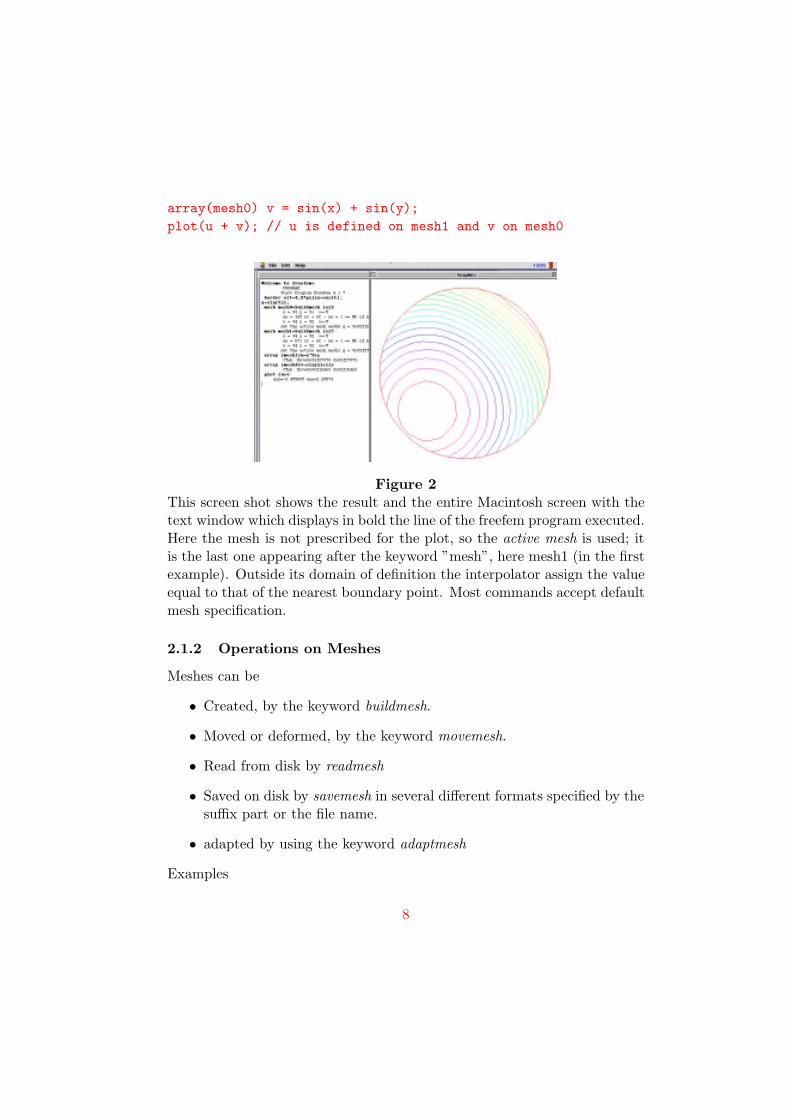
Figure 1This plot is a screen shot obtain by adding the two lines
Mesh adaption means that a finite element function u(x, y) is no longerdefined by an array of values on the vertices of a mesh but exists indepen-dantly of the mesh on which it was created. Interpolation becomes a realissue. Freefem+ provides a fast and efficient way to interpolate a functionon any mesh, it uses quadtrees, background meshes, virtual triangles... theresult is fast! You should not notice any difference in speed between the twoplots:
array(mesh1) u = x^2 + y^2;plot(mesh1,u); // plot u on its own meshplot(mesh0,u); // plot u interpolated on another mesh
How about this one:
7
array(mesh0) v = sin(x) + sin(y);plot(u + v); // u is defined on mesh1 and v on mesh0
Figure 2This screen shot shows the result and the entire Macintosh screen with thetext window which displays in bold the line of the freefem program executed.Here the mesh is not prescribed for the plot, so the active mesh is used; itis the last one appearing after the keyword ”mesh”, here mesh1 (in the firstexample). Outside its domain of definition the interpolator assign the valueequal to that of the nearest boundary point. Most commands accept defaultmesh specification.
2.1.2 Operations on Meshes
Meshes can be
• Created, by the keyword buildmesh.
• Moved or deformed, by the keyword movemesh.
• Read from disk by readmesh
• Saved on disk by savemesh in several different formats specified by thesuffix part or the file name.
• adapted by using the keyword adaptmesh
Examples
8
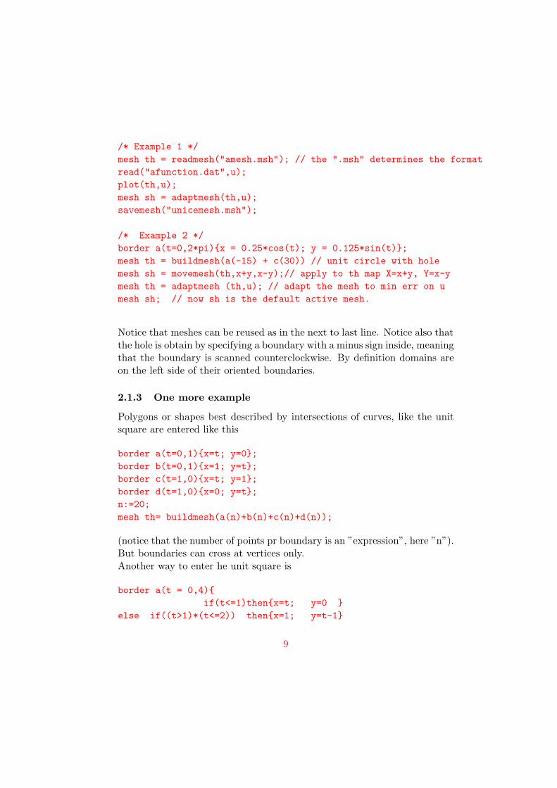
/* Example 1 */mesh th = readmesh("amesh.msh"); // the ".msh" determines the formatread("afunction.dat",u);plot(th,u);mesh sh = adaptmesh(th,u);savemesh("unicemesh.msh");
/* Example 2 */border a(t=0,2*pi)x = 0.25*cos(t); y = 0.125*sin(t);mesh th = buildmesh(a(-15) + c(30)) // unit circle with holemesh sh = movemesh(th,x+y,x-y);// apply to th map X=x+y, Y=x-ymesh th = adaptmesh (th,u); // adapt the mesh to min err on umesh sh; // now sh is the default active mesh.
Notice that meshes can be reused as in the next to last line. Notice also thatthe hole is obtain by specifying a boundary with a minus sign inside, meaningthat the boundary is scanned counterclockwise. By definition domains areon the left side of their oriented boundaries.
2.1.3 One more example
Polygons or shapes best described by intersections of curves, like the unitsquare are entered like this
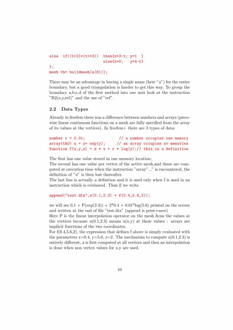
(notice that the number of points pr boundary is an ”expression”, here ”n”).But boundaries can cross at vertices only.Another way to enter he unit square is
There may be an advantage in having a single name (here ”a”) for the entireboundary, but a good triangulation is harder to get this way. To group theboundary a,b,c,d of the first method into one unit look at the instruction”R2(x,y,ref)” and the use of ”ref”.
2.2 Data Types
Already in freefem there was a difference between numbers and arrays (piece-wise linear continuous functions on a mesh are fully specified from the arrayof its values at the vertices). In freefem+ there are 3 types of data:
number r = 0.01; // a number occupies one memoryarray(th0) u = x+ exp(y); // an array occupies nv memoriesfunction f(x,y,z) = z * x + r * log(y);// this is a definition
The first has one value stored in one memory location;The second has one value per vertex of the active mesh,and these are com-puted at execution time when the instruction ”array”...” is encountered, thedefinition of ”u” is then lost thereafter.The last line is actually a definition and it is used only when f is used in aninstruction which is eveluated. Thus if we write
append("test.dta",u(0.1,2.3) + f(0.4,5.6,2));
we will see 0.1 + P(exp(2.3)) + 2*0.4 + 0.01*log(5.6) printed on the screenand written at the end of file ”test.dta” (append is print+save)Here P is the linear interpolation operator on the mesh from the values atthe vertices because u(0.1,2.3) means u(x,y) at these values : arrays areimplicit functions of the two coordinates.For f(0.4,5.6,2), the expression that defines f above is simply evaluated withthe parameters x=0.4, y=5.6, z=2. The mechanism to compute u(0.1,2.3) isentirely different, a is first computed at all vertices and then an interpolationis done when non vertex values for x,y are used.
10
2.2.1 Nearer to Math but ”racing car” Notations
We decided not to force type declaration for a data because it makes theprogram harder to read. A short form of the above is
r:= 0.01;array u = x+ exp(y);f(x,y,z) = z * x + r * log(y);
The default type is the function; to get a number one must use the := orthe ”number” qualifyer; to get an array one must explicitly use the qualifyer”array” the first time the variable is introduced. Arrays and numbers canbe reuseable but not functions. This means the following is valid
r := 0.02; // redefines r, OKarray u = x+ sin(y); // redefines u, OKg(z) = z * x + r * log(y);// same as f aboveh = x+log(y); // short for h(x,y) = x+log(y);f = x-log(y); // not allowed, redefines f
The last line will produce a compile time error because it redefines ”f”.
2.3 Partial Differential Equations
To input a PDE or a system of PDE one must use either its strong form orits weak form. Here is an example of the use of a strong form of
r:= 0.1;array u = x+y;f(x,y,z) = z * x + r * log(1+y);plot(f(x,y,0.3));
11
solve(th,w) pde(w) w - laplace(w) * 2 = f(x,y,0.3);on(c) w = u;on(b) dnu(w) + w = 1
;
plot(w);
Figure 3The results are shown on the left graphic above (the right one is the sameproblem solved by the weak form, the small differences are due to the dif-ferent quadrature formulae).Notice that on boundaries ”a” and ”d” we haven’t specified any condition;this means that it is homogeneous Neumann. Indeed, freefem builds theweak form from the data, discretizes it by the Finite Element Method ofdegree 1 on triangles and solves the discrete linear system by an LU Gaussfactorization.This is why ”dnu” is not the normal derivative but the conormal derivative,here twice the normal, i.e. for the PDE
αu+ v · ∇u−∇ · (A∇u) = f
the conormal is A n if n is the outer normal. This, by the way is the mostgeneral linear scalar second order PDE and freefem+ can solve it.The same example in weak form would be
12
varsolve(th) aa(w,W)with aa = int() (w*W + (dx(w)*dx(W)
freefem+ also handles systems (here Lam’s problem)
solve(u,v) pde(u) - laplace(u)*mu - dxx(u) - dxy(v) = f1;on(c) u = 0;pde(v) - laplace(v)*mu - dyy(v) - dyx(u) = f2;on(b) dnu(u) + v = 1;on(c) v = 0;
;
The general syntax is to write for each PDE the boundary conditions whichare naturally associated with it then the next PDE...The Stokes system in variational form is
All unknowns are followed by their corresponding test functions in the decla-ration ”varsolve”; here u1 is the test function corresponding to u... Dirichletconditions are declared by the keyword ”on” and the test function followingindicates the position of that equation in the linear system generated. Lin-ear sytems are solved by Gauss LU factorization and hence can be re-usedsuch as in
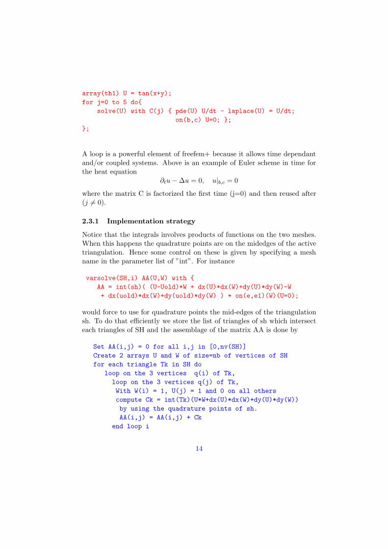
A loop is a powerful element of freefem+ because it allows time dependantand/or coupled systems. Above is an example of Euler scheme in time forthe heat equation
∂tu−∆u = 0, u|b,c = 0
where the matrix C is factorized the first time (j=0) and then reused after(j 6= 0).
2.3.1 Implementation strategy
Notice that the integrals involves products of functions on the two meshes.When this happens the quadrature points are on the midedges of the activetriangulation. Hence some control on these is given by specifying a meshname in the parameter list of ”int”. For instance
varsolve(SH,i) AA(U,W) with AA = int(sh)( (U-Uold)*W + dx(U)*dx(W)+dy(U)*dy(W)-W+ dx(uold)*dx(W)+dy(uold)*dy(W) ) + on(e,e1)(W)(U=0);
would force to use for quadrature points the mid-edges of the triangulationsh. To do that efficiently we store the list of triangles of sh which intersecteach triangles of SH and the assemblage of the matrix AA is done by
Set AA(i,j) = 0 for all i,j in [0,nv(SH)]Create 2 arrays U and W of size=nb of vertices of SHfor each triangle Tk in SH do
loop on the 3 vertices q(i) of Tk,loop on the 3 vertices q(j) of Tk,With W(i) = 1, U(j) = 1 and 0 on all otherscompute Ck = int(Tk)(U*W+dx(U)*dx(W)+dy(U)*dy(W))by using the quadrature points of sh.AA(i,j) = AA(i,j) + Ck
end loop i
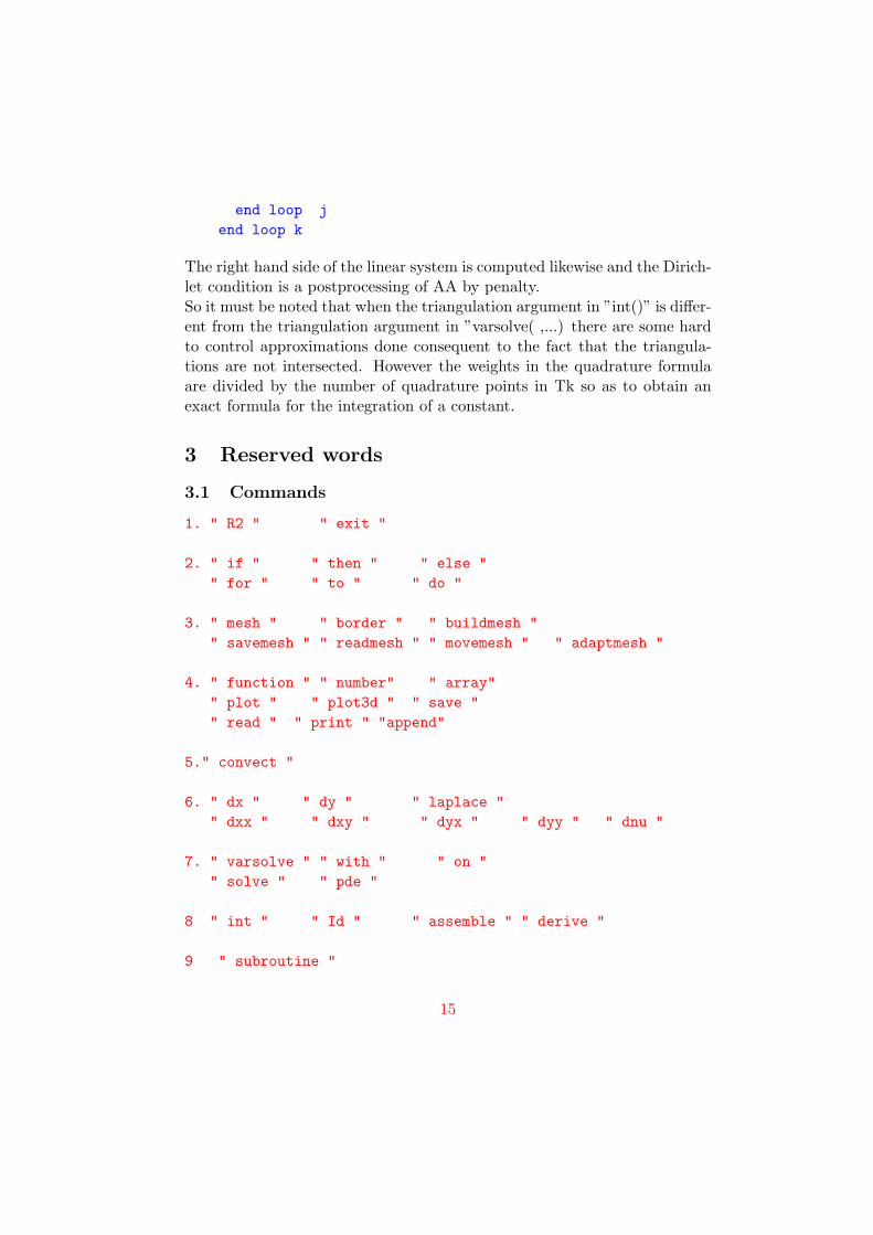
14
end loop jend loop k
The right hand side of the linear system is computed likewise and the Dirich-let condition is a postprocessing of AA by penalty.So it must be noted that when the triangulation argument in ”int()” is differ-ent from the triangulation argument in ”varsolve( ,...) there are some hardto control approximations done consequent to the fact that the triangula-tions are not intersected. However the weights in the quadrature formulaare divided by the number of quadrature points in Tk so as to obtain anexact formula for the integration of a constant.
• ”R2(x,y,ref)” means that the problem is 2D with variable x,y. Borderscan be grouped into one unit by assigning to each the same ”ref”.
• ”exit” is useful for program development.
• woX = convect(u,v,dt,w); means that w(x,y) is convected by the flowduring a time interval dt: woX(x, y) = w(X,Y ):
dX
dt= u(X,Y ),
dY
dt= v(X,Y ), X(t− δt) = x;Y (t− δt) = y.
• All the operators like dx(u) can be used inside and outside PDEs;dnu(u) is not the normal derivative of u by its conormal.
• Id(u > 1) is the Heavyside function; it is same as u > 1, only morereadible.
• ”assemble” and ”derive” are for future uses.
3.2 Reserved variables
• ”pi” = 4*atan(1.).
• ”wait”: if wait /∈ (−1, 0) graphics halt the program and the mousemust be clicked by the user. The variable wait controls also the wayplots are displaid and stored (see the section on ”plot”).
• ”nrmlx”, ”nrmly”: components of the normal. (=0 if not on boundary)
4 adaptmesh
4.1 Syntax
The syntax of the language underlying freefem, which we call Gfem , isdescribed by statements like
Here<exp> is any arithmetic expression involving functions or arrays and/orthe coordinates (x,y in general) as explicit or implicit parameters.The brackets [ ] means that the term is optional, the power n means that itcan be repeated any number of time.
16
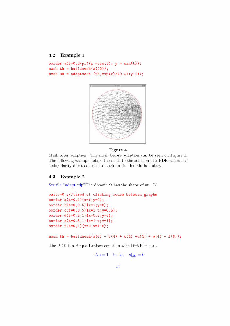
4.2 Example 1
border a(t=0,2*pi)x =cos(t); y = sin(t);mesh th = buildmesh(a(20));mesh sh = adaptmesh (th,exp(x)/(0.01+y^2));
Figure 4Mesh after adaption. The mesh before adaption can be seen on Figure 1.The following example adapt the mesh to the solution of a PDE which hasa singularity due to an obtuse angle in the domain boundary.
4.3 Example 2
See file ”adapt.edp”The domain Ω has the shape of an ”L”
wait:=0 ;//tired of clicking mouse between graphsborder a(t=0,1)x=t;y=0;border b(t=0,0.5)x=1;y=t;border c(t=0,0.5)x=1-t;y=0.5;border d(t=0.5,1)x=0.5;y=t;border e(t=0.5,1)x=1-t;y=1;border f(t=0,1)x=0;y=1-t;
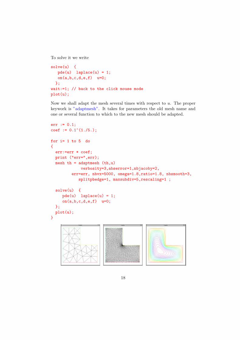
Now we shall adapt the mesh several times with respect to u. The properkeywork is ”adaptmesh”. It takes for parameters the old mesh name andone or several function to which to the new mesh should be adapted.
Figure 5The initial mesh, the final mesh, and the solution of the PDE on the finalmesh.
4.4 Example 3
See file ”fitmesh.edp”This example illustrate the power of the adaption byhessian metrics, the method underlying the mesh generator and adaptor”bang” which is used in freefem+.The idea is that the error of interpolation on a mesh is bounded by
‖u− uh‖ < C‖∇(∇u))‖h2
Therefore an attempt to keep ~hT∇(∇u)~h constant could pay. Bang doesjust that, and if you specify several function as input, like below it keeps~hT∇(∇s)∇(∇sy)~h constant. More precisely it applies the Delaunay-Voronoitriangulation algorithm with the distance function based on these Hessians(so that circles become ellpses). It is also substantially more complex be-cause, as in the example below the third function,sz, has a null Hessian, butbang has made provisions for these degenerate cases.
Figure 6Final mesh after 2 iterations, and the level lines of s (center) and sx (left)that the mesh has adapted to.
5 Expressions
Freefem+ uses regular arithmetic expressions, like most programming lan-guages. All expressions return a real value or an array of real values. As inC one can mixt booleans with reals, like x ∗ (y < 1). In addition there arenew operators.
5.1 dx,dy
Basically dx(u) is the x-derivative of u. There is some provision for formalderivatives in the language but it is not yet released, so onyl arrays can bedifferentiated.
array u = x*y;array v = dx(u);plot(y-v); // should see zero
5.2 Int
Computes integrals. It can be part of an arthmetic expression.
20
a := int(mesh0)(f+u);
It can occur in any expression; the syntax is
int([< mesh >][border[,border]n]) < expression >
• If no borders are specified it is a surface integral. Else it is a curveintegral.
• Borders can be refered by their name or their reference number.
• If the mesh is not mentionned then the default mesh is used.
• The expression may involve arrays defined on another mesh.
• The quadrature uses the mid edge of the mesh/curve.
• The curve should be made of edges which are part of the mesh else thereturn value is zero, because freefem+ loops on the edges of the meshand check if their label is in the list and add the contribution of thatedge to the result.
Warning Just like any other expressions, integrals are computed whenneeded. Hence if you write
array a = x*y - int()(x*y);
the integral will be computed 250 times if there are 250 vertices!! You shouldwrite
b:=int()(x*y);array a = x*y - b;
A similar bug, harder to catch:
f = x*y - int(x*y);....array a = f+1;
5.3 On
Used only with ”varsolve”
21
5.4 Convect
This operator performs one step of convection by the method of Characteristics-Galerkin. An equation like
∂tφ+ u∇φ = 0, φ(x, 0) = φ0(x)
is approximated by
1δt
(φn+1(x)− φn(Xn(x))) = 0
Roughly the term,φnoXn is approximated by φn(x−un(x)δt). Up to quadra-ture errors the scheme is unconditionnally stable.
• ”exp4 is the expression which is convected (u in the exemple above)
Warning ”convect” is a non local operator; in ”phi=convec(u1,u2,dt,phi0)”every values of phi0 are used to compute phi So ”phi=convec(u1,u2,dt,phi0)”won’t work won’t work.
5.4.2 Example 1
This a the rotating hill problem with one half turn. The surface (x, y, z =φ0(x, y) looks like a hill. The velociy is a pure rotation so the hill rotates.
wait:=0;border a(t=0, 2*pi)x := cos(t);y := sin(t); ;mesh th = buildmesh(a(70)); // triangulates the unit disk
• ”array” is either a new variable (which then becomes of array type oran existing array variable. There can be more than 1, up to 5 in thepresent implementation (it is easy to put more). These will be referedas ”unknowns”.
• ”with” is useful if you intend to save computing time by reusing thematrix factorized. It is imperative to check that no left hand side haschanged when you reuse a matrix, else the results will not be correct.
• ”matrix” is a new variable or a variable previously declared as a matrixi.e. appearing at the same place in a solve statement earlier.
24
• the expression after ”matrix” will be treated as a boolean (is it zeroor not?)
• if necessary regular instructions can be inserted within the solve state-ment; it is usueful if they use the arrays declared after ”solve”.
• for each unknown there must be a pde and its boundary conditions.
• each pde is restricted expression made of operators applied to any ofthe unknowns; pde(u) can involve dx(v)....
• ”borderList” is a list of names of borders separated by a comma and/ora list of integers which are the references to a set of borders.
where ”op” is a boundary operator, i.e. either any unknown or dnu(¡theUnknown¿)and ”theUnknown” is xxx the variable inside pde(xxx).
6.2 Example 1: the Stokes problem
The driven cavity flow problem is solved first at zero Reynolds numberThe velocity pressure formulation is used first and then the calculation isrepeated with the stream function vorticity formulation. The domain is theunit square
Then the system for the velocity ~u = (u, v) and the pressure p is
−∆~u+∇p = 0, ∇ · ~u = 0
25
and the boundary conditions are zero velocities except on the top boundarywhere u = 1. regularization is necessary to avoid checkerboard oscillationsso the div condition is replace by
Notice the last boundary condition which is a trick to impose ψ = 0.The problem is that we can only write boundary conditions on ω at thislevel,everything we could write on the level of the ψ equation has been done(one condition only per boundary). So by adding a tiny term ∂νω to theequation ψ = 0, the trick is plaid.
6.3 Example 2: Navier-Stokes equations
The Navier-Stokes equations offer an opportunity to illustrate the reusabilityof matrices.
∂t~u+ ~u · ∇~u− ν∆~u+∇p = 0, ∇ · ~u = 0
is approximated in time by
1δt
(un+1 − unoXn)− ν∆un+1 +∇pn+1 = 0, ∇ · un+1 = 0
The term,unoXn(x) ≈ un(x − un(x)δt) will be computed by the operator”convect”, so we obtain
nu:=0.01; dt :=0.1;for i=0 to 20 dosolve(u,v,p) with B(i)pde(u) u/dt- laplace(u)*nu + dx(p) = convect(u,v,dt,u)/dt;on(a,b,d) u =0;on(c) u = 1;pde(v) v/dt- laplace(v)*nu + dy(p) = convect(u,v,dt,v)/dt;on(a,b,c,d) v=0;pde(p) p*0.1*dt - laplace(p)*0.1*dt + dx(u)+dy(v) = 0;on(a,b,c,d) dnu(p)=0;;plot(u);;
27
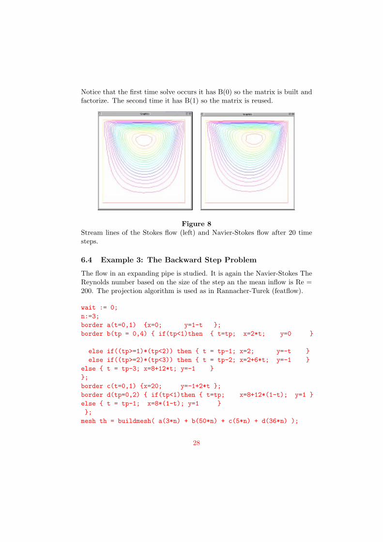
Notice that the first time solve occurs it has B(0) so the matrix is built andfactorize. The second time it has B(1) so the matrix is reused.
Figure 8Stream lines of the Stokes flow (left) and Navier-Stokes flow after 20 timesteps.
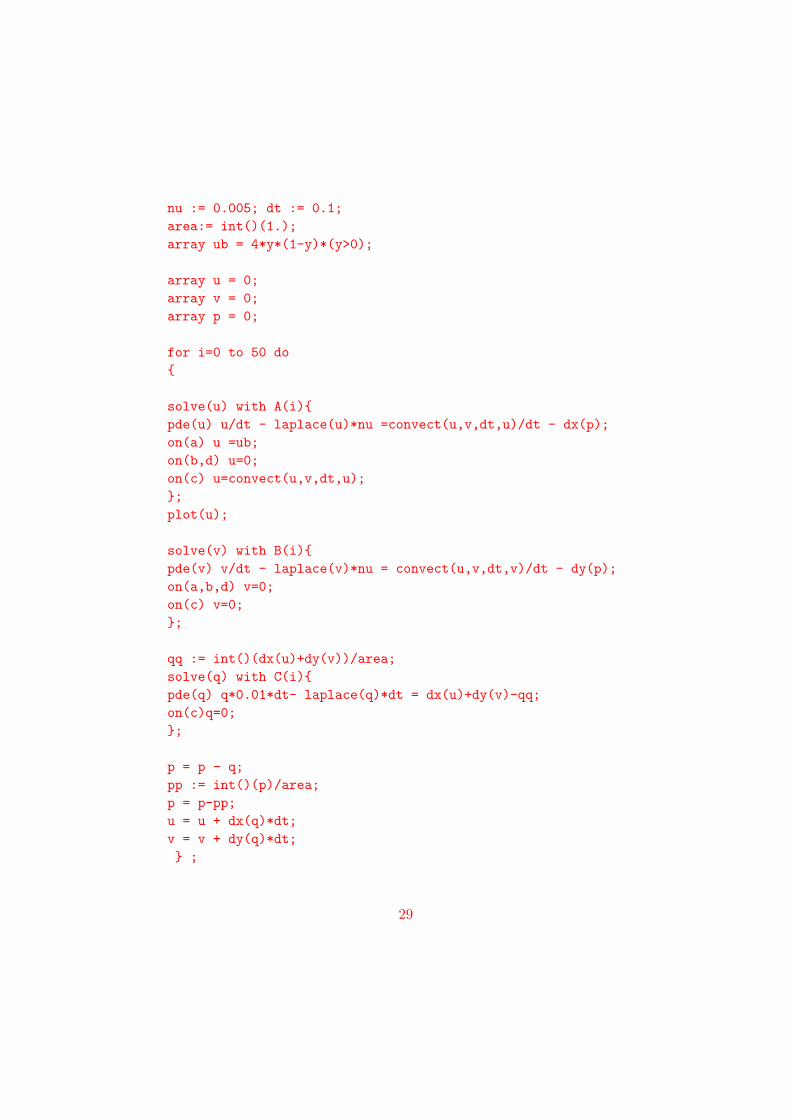
6.4 Example 3: The Backward Step Problem
The flow in an expanding pipe is studied. It is again the Navier-Stokes TheReynolds number based on the size of the step an the mean inflow is Re =200. The projection algorithm is used as in Rannacher-Turek (featflow).
qq := int()(dx(u)+dy(v))/area;solve(q) with C(i)pde(q) q*0.01*dt- laplace(q)*dt = dx(u)+dy(v)-qq;on(c)q=0;;
p = p - q;pp := int()(p)/area;p = p-pp;u = u + dx(q)*dt;v = v + dy(q)*dt; ;
29
wait:=1;plot(u);
Figure 9: The horizontal velocity after 100 time step.
7 Varsolve
This keyword triggers a very powerful feature of freefem+ where by thelinear system and right hand side of a variational equation is constructedautomatically and solved.
varsolve(th,i) aa(u,w) with aa = int()( dx(u)*dx(w)+dy(u)*dy(w)-w)+ int(a)(w*(u-g))
+ on(b,c)(w)(u=ugamma);;
If i = 0 it is used for the first time, else it is the second time it is usedand the right hand side of the variational formula (the theoretical one) haschanged only.The following should be noted:
30
• If no mesh is specified, the default mesh is used. If the mesh is specifiedit become the default mesh within the ”instruction”.
• The list of ”iden” betwen parenthesis is the variable list and the hatfunction list. Each variable is followed by its associated hat function.
• The ”instruction” should define the ”ident”. It is expected to be abilinear form in the variables. If it is not some kind of unpredictablelinearization with go on.
• The ”instruction” can be a block of instructions.
• To construct the matrix and linear system what freefem+ does is toloop on each triangle, treat all variables as hat functions, assign tothe hat functions a ”1” on one vertex, ”0” elsewhere and compute thevalue of the aa.
• The operator ”on” is a penalty operator, in this exemple it returns107w(qj)(u(qj)− uΓ(qj)) at vertex qj .
7.2 Example 1: Domain decomposition
Suppose an object Ω is made on two parts Ω = Ω1∪Ω2, Ω1∩Ω2 6= 0 and wehave a mesh for both parts but no mesh for the whole. We can still do bythe Schwarz algorithm. The idea is to compute the solution on one domainand use the value of this computation for the missing boundary conditionfor the computation on the other domain.
// Solution by Schwarz algorithmwait:=0;border a(t=0,1)x=t;y=0;border a1(t=1,2)x=t;y=0;border b(t=0,1)x=2;y=t;border c(t=2,0)x=t ;y=1;border d(t=1,0)x = 0; y = t;border e(t=0, pi/2)x= cos(t); y = sin(t);border e1(t=pi/2, 2*pi)x= cos(t); y = sin(t);n:=4;//Omega1mesh th = buildmesh( a(5*n) + a1(5*n) + b(5*n) + c(10*n) + d(5*n));//Omega2
31
mesh TH = buildmesh ( e(5*n) + e1(25*n) );//Omega1+Omega2 (only to compute the error)mesh sh = buildmesh (a1(5*n) + b(8*n) + c(10*n) + e1(25*n));
// usual FEM solutionvarsolve(sh,0) aa(uu,ww) with aa = int()( dx(uu)*dx(ww)+dy(uu)*dy(ww) - ww )+ on(a1,b,c,d,e1)(ww)(uu=0);;plot(sh,uu);
array(TH) uold=0;array(th) Uold=0;
CHI = (x^2+y^2) <= 1.0;chi = (x>=-0.01)*(y>=-0.0)*(x<=2.0)*(y<=1.0);
for i=0 to 10 dovarsolve(TH,i) AA(U,W) with AA = int(TH)( dx(U)*dx(W)+dy(U)*dy(W)-W)+ on(e,e1)(W)(U=uold*chi);;
varsolve(th,i) aa(u,w) with aa = int(th)( dx(u)*dx(w)+dy(u)*dy(w)-w)+ on(a,a1,b,c,d)(w)(u=Uold*CHI);;Uold = U*CHI;uold = u*chi;print("error=",int(th)((u-uu)^2 + (dx(u)-dx(uu))^2+(dy(u)-dy(uu))^2)+ int(TH)((U-uu)^2 + (dx(U)-dx(uu))^2+(dy(U)-dy(uu))^2) );
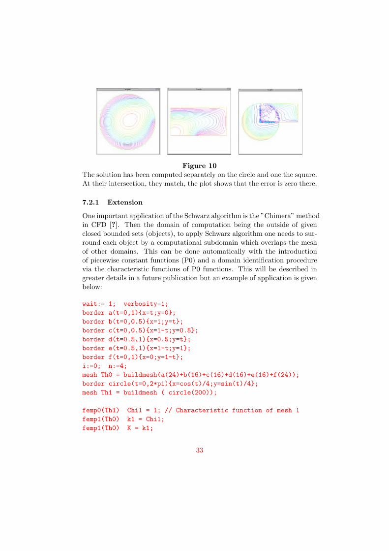
Figure 10The solution has been computed separately on the circle and one the square.At their intersection, they match, the plot shows that the error is zero there.
7.2.1 Extension
One important application of the Schwarz algorithm is the ”Chimera” methodin CFD [?]. Then the domain of computation being the outside of givenclosed bounded sets (objects), to apply Schwarz algorithm one needs to sur-round each object by a computational subdomain which overlaps the meshof other domains. This can be done automatically with the introductionof piecewise constant functions (P0) and a domain identification procedurevia the characteristic functions of P0 functions. This will be described ingreater details in a future publication but an example of application is givenbelow:
femp0(Th1) Chi1 = 1; // Characteristic function of mesh 1femp1(Th0) k1 = Chi1;femp1(Th0) K = k1;
33
plot(Th0,k1);
femp0(Th0) k0=k1;plotp0(Th0,k0>0);k1=k0; plot(Th0,k1);plotp0(Th0,k1-k0);k0=k1; plotp0 (Th1,1,Th0,k0>0);mesh Thr = Th0(k0>0,2);plot (Thr,1,Th1,2); // two plots on one screen
7.3 Example2: Fluid-Structure Interactions
We come back to the driven cavity with the Stokes equations of Example1 in the section on the keyword ”solve”. We add to it a plastic lead whichdeforms under its own weight. The box of fluid ”sh” with its lead th” ”aretriangulated as
The equations of elasticity are naturally written in variational form for thedisplacement vector u(x) ∈ V as∫
Ω[µεij(~u)εij(~w) + λtr(ε(u))tr(ε(w)] =
∫Ωf · w +
∫Γh · w, ∀w ∈ V
where ”tr” is the trace operator and with
εij(u) =12
(∂iuj + ∂jui)
The space V may contain constraints of Dirichlet type if the structure isclamped on part of its boundary. Here we assume that the lead is clampedon its vertical sides and that the only force is the gravity. Then the systemis solved by
The last line allows us to see the deformed structure. As we intend to reusethe matrix of the linear system and avoid factorization, we use a zero in theparameter.When the fluid rotates the lid of the cavity is subject to the normal stressdue to the fluid.
σn = ∇u+∇uT − pn
This surfacic force acts on the structure and deforms it. Now to include theeffect of the fluid surface stress we solve
varsolve(1) bb(uu,w,vv,s) with bb = int()( 2*mu*(e11*w11+e12*w12+e22*w22)
The ”mesh” is the one which determines the domain on which the functionis plotted. It does not have to be the one on which the function(s) is(are)defined.By translations (movemesh) one can control the layout of the plots.
8.1.1 Zooms and plots
Graphics may flow continuously or may halt the program to allow the userto study them. If wait ∈ [−1, 0] graphics do not halt the program. The”graphic window” is initialized at startup so that the domain fits and iscentered in the graphic window. If wait is active (i.e. wait /∈ [−1, 0]) thenwhile a graphic is displaid the user can redefine the layout of the graphic inthe graphic window by typing +,− or =.
36
If + (resp -) is typed the graphic is zoomed (resp unzoomed) around theposition of the cursor. If = is typed then the graphic position is reinitialzedto what it was at startup.
8.1.2 Plots and the variable ”wait”
If wait is active then it is possible to redefine it by typing
• r 0 : then no subsequent graphics will halt the program
• r 1 : all subsequent graphics will halt the program
• r -1 no subsequent graphics will halt the program and the graphicwindow is reinitialized to its values at startup.
• r -2 : all subsequent graphics will halt the program and the graphicwindow is reinitialized to its values at startup.
8.2 Summary of keyboard commands
If wait is active only:
• <Control> c : stops the program
• r : redraws the graphic
• r and 1,0,-1,-2: redraws the graphic and redefines ”wait” to the typedvalue (if in wait active mode)
• + : zoom in the current graphic and all subsequent ones (if in waitactive mode)
• - : unzoom the current graphic and all subsequent ones (if in waitactive mode)
• = : reinitialize the current graphic and all subsequent ones (if in waitactive mode)
37
8.3 The keywords ”readmesh”, ”savemesh”,”read” and ”save”
There are a number of formats to save meshes and arrays and freefem re-spond to the suffixe of the file name given.
savemesh(” < filename > ”[, < meshname >])
The string is the file name and if no mesh is specified then the defaultmesh is used. The filename is xxx or xxx.xxx where xxx is any number ofalphanumeric character. The last part after the ”.” is the suffix, if any. Bydefault the format is the same as in freefem 3.0.
mesh < name >= readmesh(” < filename > ”)
Mesh file formats are
• .amdba the INRIA amdba format
• .msh the freefem format
• .am fmt the EMC2 INRIA format
Note triangulations are not renumbered by the read statement. Labels forboundaries remain numerical but they can be used as label in statementslike ”on(4,5)....”.
Other data file format are
• .dbg an extended talkative format for debugging (savemesh only)
• .gnu a format to plot 3D surfaces with gnuplot ”with lines”. (saveonly)
• .ps a format to save the equivalent graphic (with its zoomed options)in PostScript
save(” < filename > ”, < arrayname >)
Saves in ¡filename¿ a function named ¡arrayname¿ on the active triangula-tion.
read(” < filename > ”, < arrayname >)
Reads from ¡filename¿ a function named ¡arrayname¿ on the active triangu-lation.
38
8.4 Save displaid plots
This section applies to the 3 keywords ”plot”, ”buildmesh”, ”adaptmesh”.
It is useful to be able to save graphics as displaid, in PostScript format.This can be done by putting a file name in the parameter list of the instruc-tion plot.Exampleplot(”f.ps”,th,f);
It is also useful to save a graphic withing an iteration loops. Then thefilename must change at each loop. There is provision for this by using afile name in the format
” < string > ” < var > ” < string”
Example
for i=0 to 10 do
varsolve(TH,i) AA(U,W) with .... // defines U
plot(U);save("U_"i".ps",U);
9 Application: Domain Decomposition
We recently ran into the following problem: is it possible to solve a PDE ina domain Ω − O where O is a hole in the domain without ever having togenerate the triangulation of Ω−O ?Here is an answer (Lions et al [1]).Let V = H1
0 (Ω). we look for u ∈ V such that∫Ω∇u∇v =
∫Ωfv ∀v ∈ V
Assume that Ω ait un trou O. Let Ω1 = Ω and let Ω2 be an open set thatcontains O and is contained in Ω1 Let Vi = H1
0 (Ωi) .
39
Algorithm Loop on un+11 ∈ V1 such that∫
Ω1
∇un+11 ∇v1 +
∫Ω12
∇un2∇v1 =∫
Ω1
fv1, ∀v1 ∈ V1
and loop on un+12 + un1 ∈ V2 such that∫
Ω2
∇un+12 ∇v2 +
∫Ω12
∇un2∇v2 =∫
Ω2
fv2, ∀vi ∈ Vi
The following program is an application of this idea to a schematic conterthall (Helmholtz equation) where rows of seats are inserted. The mesh of theconcert hall with the seats is not needed except to check the results.
Figure 12The full solution (right) is obtained by superposition of the local solutionsnear the holes (left) withthe solution in the big domain without the holes(middle).
10 References
1. J.L. Lions, O. Pironneau: Superpositions for composite domains (toappear)
2. B. Lucquin, O. Pironneau: Scientific Computing for Engineers Wiley1998.”


![[hal-00694787, v1] FreeFem++, a tool to solve PDEs numericallycalcul.math.cnrs.fr/Documents/Ecoles/LEM2I/Mod4/FreeFempp.pdf · FreeFem ++, a tool to solve PDEs numerically Georges](https://static.documents.pub/doc/80x56/5b012a507f8b9ab9598be717/hal-00694787-v1-freefem-a-tool-to-solve-pdes-a-tool-to-solve-pdes-numerically.jpg)


