Page 1
The problem: Dynamics of soliton in NLS with external potential Main Theorem Scheme of the proof
Freezing of energy of a soliton in an externalpotential
A. Maspero∗
joint work with D. Bambusi
∗Laboratoire de Mathematiques Jean Leray - Universite de Nantes, Nantes
November 27, 2015, Nantes
Page 2
The problem: Dynamics of soliton in NLS with external potential Main Theorem Scheme of the proof
Outline
1 The problem: Dynamics of soliton in NLS with external potential
2 Main Theorem
3 Scheme of the proof
Page 3
The problem: Dynamics of soliton in NLS with external potential Main Theorem Scheme of the proof
The equation
NLS with small external potential V
i∂tψ = −∆ψ − β′(|ψ|2)ψ + εV (x)ψ , x ∈ R3 ,
V Schwartz class
β focusing nonlinearity, β ∈ C∞(R,R)∣∣∣β(k)(u)∣∣∣ ≤ Ck 〈u〉1+p−k
, β′(0) = 0 p < 2/3 ,
Under this assumptions: global unique solution for initial data in H1
Problem: effective dynamics of solitary waves solutions
Page 4
The problem: Dynamics of soliton in NLS with external potential Main Theorem Scheme of the proof
Case ε = 0
Look for moving solitary waves:
ψ(x , t) = eiγ(t)eip(t)·(x−q(t))/m(t)ηm(t)(x − q(t))
where ηm is the ground state of NLS with mass m, and p, q ∈ R3, γ ∈ Rtime-dependent parameter which fulfill
p = 0
q = pm
m = 0
γ = E(m) + |p|24m
(1)
Invariant 8-dimensional symplectic manifold of solitary waves:
T =⋃
p,q∈R3
γ∈R,m∈I
eiγeip·(x−q)/mηm(x − q)
Solitary wave travels through space with constant velocity
hamiltonian equations of free mechanical particle
Page 5
The problem: Dynamics of soliton in NLS with external potential Main Theorem Scheme of the proof
Case ε 6= 0
T is not longer invariant. ”Symplectic Decomposition”:
ψ = e iγeip·(x−q)/mηm(· − q) + φ(x , t)
with time-dependent parameter p(t), q(t), γ(t),m(t) fulfillingp = −ε∇V eff (q) +O(ε2)
q = pm +O(ε2)
m = O(ε2)
γ = E(m) + |p|24m − εV
eff (q) +O(ε2)
(2)
with V eff (q) =∫R3 V (x + q) η2
m dxfirst two equations are hamiltonian equations of mechanical particle interactingwith external field
Hεmech(p, q) =|p|2
2m+ εV eff (q)
Solitary waves moves ”like a mechanical particle in an external potential”
for which interval of time is the argument rigorous?
Page 6
The problem: Dynamics of soliton in NLS with external potential Main Theorem Scheme of the proof
Case ε 6= 0
T is not longer invariant. ”Symplectic Decomposition”:
ψ = e iγeip·(x−q)/mηm(· − q) + φ(x , t)
with time-dependent parameter p(t), q(t), γ(t),m(t) fulfillingp = −ε∇V eff (q) +O(ε2)
q = pm +O(ε2)
m = O(ε2)
γ = E(m) + |p|24m − εV
eff (q) +O(ε2)
(2)
with V eff (q) =∫R3 V (x + q) η2
m dxfirst two equations are hamiltonian equations of mechanical particle interactingwith external field
Hεmech(p, q) =|p|2
2m+ εV eff (q)
Solitary waves moves ”like a mechanical particle in an external potential”
for which interval of time is the argument rigorous?
Page 7
The problem: Dynamics of soliton in NLS with external potential Main Theorem Scheme of the proof
Previous results
Frohlich-Gustafson-Jonsson-Sigal ’04, ’06, Holmer-Zworski ’08:
dist(
(p(t), q(t)), (pmech(t), qmech(t))) ε1/2 for times |t| ≤ T ε−3/2
Question: can we do better? Answer: NO!
Page 8
The problem: Dynamics of soliton in NLS with external potential Main Theorem Scheme of the proof
Previous results
Frohlich-Gustafson-Jonsson-Sigal ’04, ’06, Holmer-Zworski ’08:
dist(
(p(t), q(t)), (pmech(t), qmech(t))) ε1/2 for times |t| ≤ T ε−3/2
Question: can we do better? Answer: NO!
Page 9
The problem: Dynamics of soliton in NLS with external potential Main Theorem Scheme of the proof
Previous results
Frohlich-Gustafson-Jonsson-Sigal ’04, ’06, Holmer-Zworski ’08:
dist(
(p(t), q(t)), (pmech(t), qmech(t))) ε1/2 for times |t| ≤ T ε−3/2
Question: can we do better? Answer: NO!
true motions of the soliton are actually different from themechanical ones and the difference becomes macroscopic after aquite short time scale
Page 10
The problem: Dynamics of soliton in NLS with external potential Main Theorem Scheme of the proof
New point of view
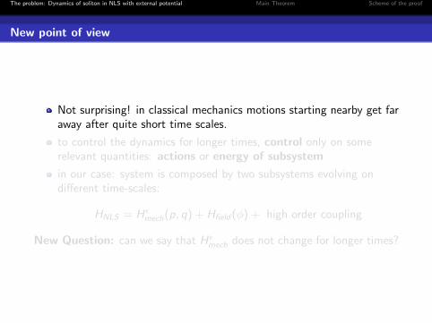
Not surprising! in classical mechanics motions starting nearby get faraway after quite short time scales.
to control the dynamics for longer times, control only on somerelevant quantities: actions or energy of subsystem
in our case: system is composed by two subsystems evolving ondifferent time-scales:
HNLS = Hεmech(p, q) + Hfield (φ) + high order coupling
New Question: can we say that Hεmech does not change for longer times?
Page 11
The problem: Dynamics of soliton in NLS with external potential Main Theorem Scheme of the proof
New point of view
Not surprising! in classical mechanics motions starting nearby get faraway after quite short time scales.
to control the dynamics for longer times, control only on somerelevant quantities: actions or energy of subsystem
in our case: system is composed by two subsystems evolving ondifferent time-scales:
HNLS = Hεmech(p, q) + Hfield (φ) + high order coupling
New Question: can we say that Hεmech does not change for longer times?
Page 12
The problem: Dynamics of soliton in NLS with external potential Main Theorem Scheme of the proof
New point of view
Not surprising! in classical mechanics motions starting nearby get faraway after quite short time scales.
to control the dynamics for longer times, control only on somerelevant quantities: actions or energy of subsystem
in our case: system is composed by two subsystems evolving ondifferent time-scales:
HNLS = Hεmech(p, q) + Hfield (φ) + high order coupling
New Question: can we say that Hεmech does not change for longer times?
Page 13
The problem: Dynamics of soliton in NLS with external potential Main Theorem Scheme of the proof
New point of view
Not surprising! in classical mechanics motions starting nearby get faraway after quite short time scales.
to control the dynamics for longer times, control only on somerelevant quantities: actions or energy of subsystem
in our case: system is composed by two subsystems evolving ondifferent time-scales:
HNLS = Hεmech(p, q) + Hfield (φ) + high order coupling
New Question: can we say that Hεmech does not change for longer times?
Page 14
The problem: Dynamics of soliton in NLS with external potential Main Theorem Scheme of the proof
Outline
1 The problem: Dynamics of soliton in NLS with external potential
2 Main Theorem
3 Scheme of the proof
Page 15
The problem: Dynamics of soliton in NLS with external potential Main Theorem Scheme of the proof
Assumptions
Linearization at the soliton: χ = L0χWe assume
1 σd (L0) = 0, σc (L0) =⋃±±i[E ,±∞)
2 Ker(L+) = span(ηm) , Ker(L−) = span(∂xjηm)j=1,...,3, 0 hasmultiplicity 8
3 ±iE are not resonances, i.e. L0χ = iEχ has no solution with〈x〉−δ χ ∈ L2,∀δ > 1/2
Page 16
The problem: Dynamics of soliton in NLS with external potential Main Theorem Scheme of the proof
Theorem (Bambusi, M.)
Fix arbitrary r ∈ N. Then ∃εr s.t. for 0 ≤ ε < εr , it holds the following:∀ψ0 ∈ H1 with
‖ψ0 − eiαηm(p, q)‖H1 ≤ K1ε1/2
Hεmech(p, q) < K2ε ,
(3)
then the solution ψ(t) admits the decomposition in H1
ψ(t) := eiα(t)ηm(p(t),q(t)) + φ(t) , (4)
with a constant m and smooth functions p(t),q(t), α(t) s.t.
|Hεmech(p(t),q(t))− Hε
mech(p(0),q(0))| ≤ C1ε3/2 , |t| ≤ T0
εr. (5)
Furthermore, for the same times one has
‖φ(t)‖H1 ≤ C1ε1/2 .
Page 17
The problem: Dynamics of soliton in NLS with external potential Main Theorem Scheme of the proof
Some remarks
the energy of the soliton freezes for times ∼ ε−r
Key point: frequency of the soliton ∼ ε1/2, frequency of the field ∼ 1
assume that V and ψ0 are symmetric around an axis, then themechanical hamiltonian is 1-dimensional. Then one can control alsothe orbit of the soliton
Page 18
The problem: Dynamics of soliton in NLS with external potential Main Theorem Scheme of the proof
Outline
1 The problem: Dynamics of soliton in NLS with external potential
2 Main Theorem
3 Scheme of the proof
Page 19
The problem: Dynamics of soliton in NLS with external potential Main Theorem Scheme of the proof
Main steps
1) Canonical variables (Darboux theorem ):
- ψ = eqj JAj (ηp + φ), but p, q, φ not canonical- Darboux theorem: canonical p′, q′, φ′ in a neighborhood of T
2) Birkhoff normal form (continuous spectrum)
- in Darboux coordinates
H = ε1/2Hmech(p′, q′) +1
2
⟨EL0φ
′, φ′⟩
+ ε3/4⟨Ψ(p′, q′), φ′
⟩+ h.o.t.
- cancel terms linear in φ′ up to order εr
3) dispersive estimates (Strichartz)
- φ = L0φ+ B(t)φ+ εr Ψ + h.o.t.with B(t) time-dependent unbounded operator
- Strichartz stable: ‖φ‖L2
t [0,T ]W1,6x
+ ‖φ‖L∞t [0,T ]H1x≤ Kε1/2 , ∀|t| ≤ T ε−r
- almost conservation of energy
|HL(φ(t))− HL(φ(0))| ≤ ε ∀|t| ≤ T ε−r
Page 20
The problem: Dynamics of soliton in NLS with external potential Main Theorem Scheme of the proof
Main steps
1) Canonical variables (Darboux theorem ):
- ψ = eqj JAj (ηp + φ), but p, q, φ not canonical- Darboux theorem: canonical p′, q′, φ′ in a neighborhood of T
2) Birkhoff normal form (continuous spectrum)
- in Darboux coordinates
H = ε1/2Hmech(p′, q′) +1
2
⟨EL0φ
′, φ′⟩
+ ε3/4⟨Ψ(p′, q′), φ′
⟩+ h.o.t.
- cancel terms linear in φ′ up to order εr
3) dispersive estimates (Strichartz)
- φ = L0φ+ B(t)φ+ εr Ψ + h.o.t.with B(t) time-dependent unbounded operator
- Strichartz stable: ‖φ‖L2
t [0,T ]W1,6x
+ ‖φ‖L∞t [0,T ]H1x≤ Kε1/2 , ∀|t| ≤ T ε−r
- almost conservation of energy
|HL(φ(t))− HL(φ(0))| ≤ ε ∀|t| ≤ T ε−r
Page 21
The problem: Dynamics of soliton in NLS with external potential Main Theorem Scheme of the proof
Main steps
1) Canonical variables (Darboux theorem ):
- ψ = eqj JAj (ηp + φ), but p, q, φ not canonical- Darboux theorem: canonical p′, q′, φ′ in a neighborhood of T
2) Birkhoff normal form (continuous spectrum)
- in Darboux coordinates
H = ε1/2Hmech(p′, q′) +1
2
⟨EL0φ
′, φ′⟩
+ ε3/4⟨Ψ(p′, q′), φ′
⟩+ h.o.t.
- cancel terms linear in φ′ up to order εr
3) dispersive estimates (Strichartz)
- φ = L0φ+ B(t)φ+ εr Ψ + h.o.t.with B(t) time-dependent unbounded operator
- Strichartz stable: ‖φ‖L2
t [0,T ]W1,6x
+ ‖φ‖L∞t [0,T ]H1x≤ Kε1/2 , ∀|t| ≤ T ε−r
- almost conservation of energy
|HL(φ(t))− HL(φ(0))| ≤ ε ∀|t| ≤ T ε−r
Page 22
The problem: Dynamics of soliton in NLS with external potential Main Theorem Scheme of the proof
Framework
Phase space:
Hs,k , scale of Hilbert spaces, ‖ψ‖Hs,k = ‖ 〈x〉s (∆− 1)k/2ψ‖L2
〈ψ1;ψ2〉 = 2Re∫ψ1ψ2
ω(ψ1, ψ2) := 〈Eψ1;ψ2〉, with E = i, J = E−1 Poisson tensor
Symmetries:
Aj := i∂xj , j = 1, 2, 3, A4 = 1,
eqj JAjψ ≡ ψ(· − qj ej )
Soliton manifold: T :=⋃q,p
eqj JAj ηp , where ηp := ei
pk xk
p4 ηp4
restriction ω|T = dp ∧ dq
Natural decomposition:
L2 ≡ Tηp L2 ' TηpT ⊕ T∠ηpT
with T∠ηpT :=
U : ω(U; X ) = 0 , ∀X ∈ TηpT
Let Πp : L2 → T∠
ηpT the projector on the symplectic orthogonal
Page 23
The problem: Dynamics of soliton in NLS with external potential Main Theorem Scheme of the proof
Framework
Phase space:
Hs,k , scale of Hilbert spaces, ‖ψ‖Hs,k = ‖ 〈x〉s (∆− 1)k/2ψ‖L2
〈ψ1;ψ2〉 = 2Re∫ψ1ψ2
ω(ψ1, ψ2) := 〈Eψ1;ψ2〉, with E = i, J = E−1 Poisson tensor
Symmetries:
Aj := i∂xj , j = 1, 2, 3, A4 = 1,
eqj JAjψ ≡ ψ(· − qj ej )
Soliton manifold: T :=⋃q,p
eqj JAj ηp , where ηp := ei
pk xk
p4 ηp4
restriction ω|T = dp ∧ dq
Natural decomposition:
L2 ≡ Tηp L2 ' TηpT ⊕ T∠ηpT
with T∠ηpT :=
U : ω(U; X ) = 0 , ∀X ∈ TηpT
Let Πp : L2 → T∠
ηpT the projector on the symplectic orthogonal
Page 24
The problem: Dynamics of soliton in NLS with external potential Main Theorem Scheme of the proof
Framework
Phase space:
Hs,k , scale of Hilbert spaces, ‖ψ‖Hs,k = ‖ 〈x〉s (∆− 1)k/2ψ‖L2
〈ψ1;ψ2〉 = 2Re∫ψ1ψ2
ω(ψ1, ψ2) := 〈Eψ1;ψ2〉, with E = i, J = E−1 Poisson tensor
Symmetries:
Aj := i∂xj , j = 1, 2, 3, A4 = 1,
eqj JAjψ ≡ ψ(· − qj ej )
Soliton manifold: T :=⋃q,p
eqj JAj ηp , where ηp := ei
pk xk
p4 ηp4
restriction ω|T = dp ∧ dq
Natural decomposition:
L2 ≡ Tηp L2 ' TηpT ⊕ T∠ηpT
with T∠ηpT :=
U : ω(U; X ) = 0 , ∀X ∈ TηpT
Let Πp : L2 → T∠
ηpT the projector on the symplectic orthogonal
Page 25
The problem: Dynamics of soliton in NLS with external potential Main Theorem Scheme of the proof
Framework
Phase space:
Hs,k , scale of Hilbert spaces, ‖ψ‖Hs,k = ‖ 〈x〉s (∆− 1)k/2ψ‖L2
〈ψ1;ψ2〉 = 2Re∫ψ1ψ2
ω(ψ1, ψ2) := 〈Eψ1;ψ2〉, with E = i, J = E−1 Poisson tensor
Symmetries:
Aj := i∂xj , j = 1, 2, 3, A4 = 1,
eqj JAjψ ≡ ψ(· − qj ej )
Soliton manifold: T :=⋃q,p
eqj JAj ηp , where ηp := ei
pk xk
p4 ηp4
restriction ω|T = dp ∧ dq
Natural decomposition:
L2 ≡ Tηp L2 ' TηpT ⊕ T∠ηpT
with T∠ηpT :=
U : ω(U; X ) = 0 , ∀X ∈ TηpT
Let Πp : L2 → T∠
ηpT the projector on the symplectic orthogonal
Page 26
The problem: Dynamics of soliton in NLS with external potential Main Theorem Scheme of the proof
Step 1: Canonical variables
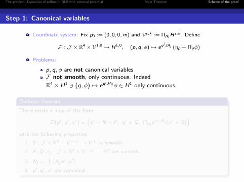
Coordinate system: Fix p0 := (0, 0, 0,m) and Vs,k := Πp0 Hs,k . Define
F : J × R4 × V1,0 → H1,0, (p, q, φ) 7→ eqj JAj (ηp + Πpφ)
Problems:
p, q, φ are not canonical variablesF not smooth, only continuous. Indeed
R4 × H1 3 (q, φ) 7→ eqj JAjφ ∈ H1 only continuous
Darboux theorem
There exists a map of the form
D(p′, q′, φ′) =(
p′ − N + P, q′ + Q, Πp0 eαj JAj (φ′ + S)),
with the following properties
1. S : J × R4 × V−∞ → V∞ is smooth.
2. P,Q, αj : J × R4 × V−∞ → R4 are smooth.
3. Nj := 12
⟨Ajφ′, φ′
⟩4. p′, q′, φ′ are canonical.
Page 27
The problem: Dynamics of soliton in NLS with external potential Main Theorem Scheme of the proof
Step 1: Canonical variables
Coordinate system: Fix p0 := (0, 0, 0,m) and Vs,k := Πp0 Hs,k . Define
F : J × R4 × V1,0 → H1,0, (p, q, φ) 7→ eqj JAj (ηp + Πpφ)
Problems:
p, q, φ are not canonical variablesF not smooth, only continuous. Indeed
R4 × H1 3 (q, φ) 7→ eqj JAjφ ∈ H1 only continuous
Darboux theorem
There exists a map of the form
D(p′, q′, φ′) =(
p′ − N + P, q′ + Q, Πp0 eαj JAj (φ′ + S)),
with the following properties
1. S : J × R4 × V−∞ → V∞ is smooth.
2. P,Q, αj : J × R4 × V−∞ → R4 are smooth.
3. Nj := 12
⟨Ajφ′, φ′
⟩4. p′, q′, φ′ are canonical.
Page 28
The problem: Dynamics of soliton in NLS with external potential Main Theorem Scheme of the proof
Proof of the Darboux theorem
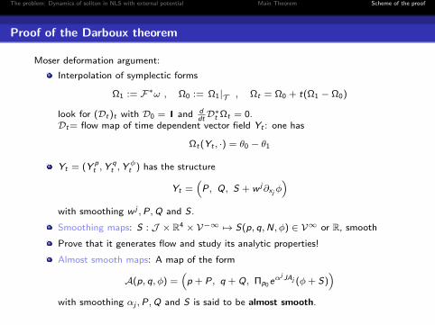
Moser deformation argument:
Interpolation of symplectic forms
Ω1 := F∗ω , Ω0 := Ω1|T , Ωt = Ω0 + t(Ω1 − Ω0)
look for (Dt )t with D0 = 1 and ddtD∗t Ωt = 0.
Dt = flow map of time dependent vector field Yt : one has
Ωt (Yt , ·) = θ0 − θ1
Yt = (Y pt ,Y
qt ,Y
φt ) has the structure
Yt =(
P, Q, S + w j∂xjφ)
with smoothing w j ,P,Q and S .
Smoothing maps: S : J × R4 × V−∞ 7→ S(p, q,N, φ) ∈ V∞ or R, smooth
Prove that it generates flow and study its analytic properties!
Almost smooth maps: A map of the form
A(p, q, φ) =(
p + P, q + Q, Πp0 eαj JAj (φ+ S)
)with smoothing αj ,P,Q and S is said to be almost smooth.
Page 29
The problem: Dynamics of soliton in NLS with external potential Main Theorem Scheme of the proof
Step 2: The Hamiltonian in Darboux coordinates and normal form
Hamiltonian in Darboux coordinates: Let D be the Darboux map. Then
H F D = ε1/2h + HL + ε3/4HR
with
h =p2
2m+ V eff (q), HL =
1
2〈EL0φ, φ〉
and
dφHR (0)[φ] = 〈S , φ〉 , S(p, q,N) smoothing (Nj =1
2
⟨i∂xjφ, φ
⟩)
Birkhoff normal form: eliminate terms linear in φ up to order r in ε.
Lie transform: flow map of χr = εr⟨χ(r)(N, p, q), φ
⟩Homological equation: L0χ
(r) = S , L0 with continuous spectrum
Flow: hamiltonian vector field of χr is not smooth
Xχr =(
P, Q, S + w j∂xjφ)
It generates an almost smooth map, furthermore H F D A has the samestructure, but with terms linear in φ at order εr+1
Page 30
The problem: Dynamics of soliton in NLS with external potential Main Theorem Scheme of the proof
Step 2: The Hamiltonian in Darboux coordinates and normal form
Hamiltonian in Darboux coordinates: Let D be the Darboux map. Then
H F D = ε1/2h + HL + ε3/4HR
with
h =p2
2m+ V eff (q), HL =
1
2〈EL0φ, φ〉
and
dφHR (0)[φ] = 〈S , φ〉 , S(p, q,N) smoothing (Nj =1
2
⟨i∂xjφ, φ
⟩)
Birkhoff normal form: eliminate terms linear in φ up to order r in ε.
Lie transform: flow map of χr = εr⟨χ(r)(N, p, q), φ
⟩Homological equation: L0χ
(r) = S , L0 with continuous spectrum
Flow: hamiltonian vector field of χr is not smooth
Xχr =(
P, Q, S + w j∂xjφ)
It generates an almost smooth map, furthermore H F D A has the samestructure, but with terms linear in φ at order εr+1
Page 31
The problem: Dynamics of soliton in NLS with external potential Main Theorem Scheme of the proof
Step 3: Analysis of the normal form
We have H T r+2 in normal form at order r + 2.
φ = L0φ+ ε3/4B(t)φ+ εr+2S + h.o.t.
and B(t) = w j (t)∂xj + V (x , t) time-dependent unbounded linear operator
Aim: Nonlinear stability for φ!
Remark: linearized equation has time-dependent unbounded operator: a disaster on acompact manifold!
Miracle: on Rn, Strichartz
Strichartz stable under some unbounded small perturbations (Perelman,Beceanu):
‖φ‖L2
t [0,T ]W1,6x
+ ‖φ‖L∞t [0,T ]H1x≤ Kε1/4 , ∀|t| ≤ T ε−r
Using this, one proves that
|HL(φ(t))− HL(φ(0))| ≤ ε ∀|t| ≤ T ε−r
conservation of energy implies conservation of Hεmech
Page 32
The problem: Dynamics of soliton in NLS with external potential Main Theorem Scheme of the proof
Step 3: Analysis of the normal form
We have H T r+2 in normal form at order r + 2.
φ = L0φ+ ε3/4B(t)φ+ εr+2S + h.o.t.
and B(t) = w j (t)∂xj + V (x , t) time-dependent unbounded linear operator
Aim: Nonlinear stability for φ!
Remark: linearized equation has time-dependent unbounded operator: a disaster on acompact manifold!
Miracle: on Rn, Strichartz
Strichartz stable under some unbounded small perturbations (Perelman,Beceanu):
‖φ‖L2
t [0,T ]W1,6x
+ ‖φ‖L∞t [0,T ]H1x≤ Kε1/4 , ∀|t| ≤ T ε−r
Using this, one proves that
|HL(φ(t))− HL(φ(0))| ≤ ε ∀|t| ≤ T ε−r
conservation of energy implies conservation of Hεmech
Page 33
The problem: Dynamics of soliton in NLS with external potential Main Theorem Scheme of the proof
Thanks for your attention!