56
Frequency distributions: Testing of goodness of fit and contingency tables
| Date post: | 22-Dec-2015 |
| Category: |
Documents |
| View: | 240 times |
| Download: | 2 times |

Frequency distributions: Testing of goodness of fit and contingency tables
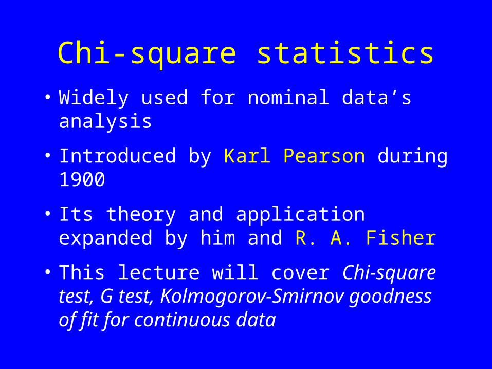
Chi-square statistics• Widely used for nominal data’s
analysis
• Introduced by Karl Pearson during 1900
• Its theory and application expanded by him and R. A. Fisher
• This lecture will cover Chi-square test, G test, Kolmogorov-Smirnov goodness of fit for continuous data
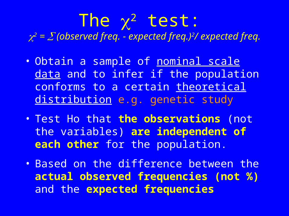
The 2 test: 2 = (observed freq. - expected freq.)2/ expected freq.
• Obtain a sample of nominal scale data and to infer if the population conforms to a certain theoretical distribution e.g. genetic study
• Test Ho that the observations (not the variables) are independent of each other for the population.
• Based on the difference between the actual observed frequencies (not %) and the expected frequencies

The 2 test: 2 = (observed freq. - expected freq.)2/ expected freq.
• As a measure of how far a sample distribution deviates from a theoretical distribution
• Ho: no difference between the observed and expected frequency (HA: they are different)
• If Ho is true: the difference and Chi-square SMALL
• If Ho is false: both measurements Large
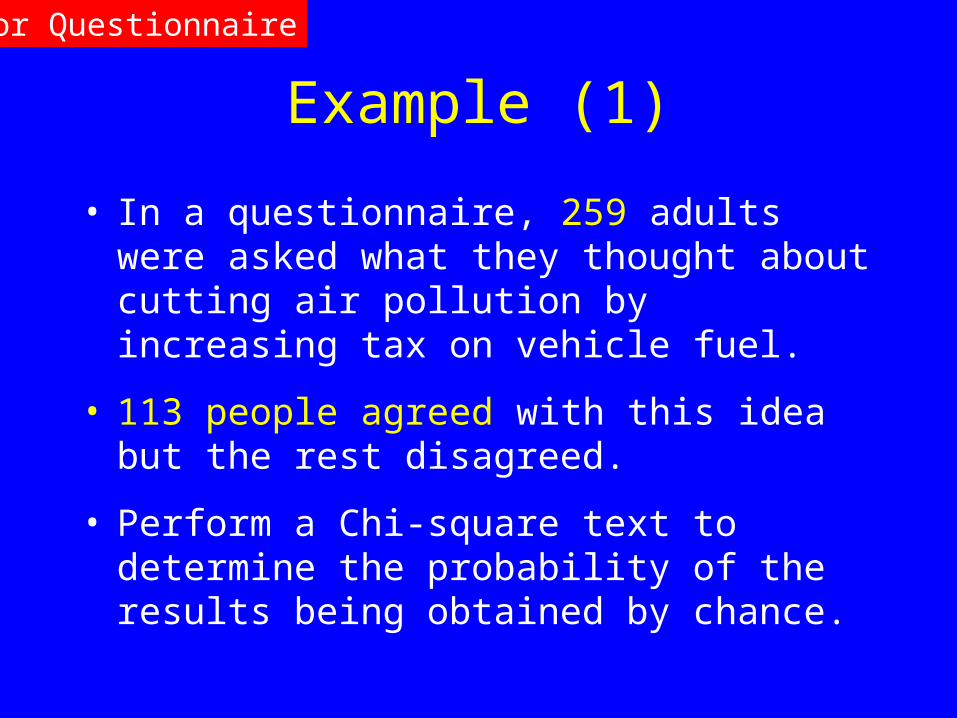
Example (1)
• In a questionnaire, 259 adults were asked what they thought about cutting air pollution by increasing tax on vehicle fuel.
• 113 people agreed with this idea but the rest disagreed.
• Perform a Chi-square text to determine the probability of the results being obtained by chance.
For Questionnaire

Agree Disagree
Observed 113 259 -113 = 146
Expected 259/2 = 129.5 259/2 = 129.5
Ho: Observed = Expected
2 = (113 - 129.5)2/129.5 + (146 - 129.5)2 /129.5
= 2.102 + 2.102 = 4.204
df = k - 1 = 2 - 1 = 1
From the Chi-square (Table B1 in Zar’s book)
2 ( = 0.05, df = 1)= 3.841 for 2 = 4.202, 0.025<p<0.05
Therefore, rejected Ho. The probability of the results being obtained by chance is between 0.025 and 0.05.
For Questionnaire

Practical (1)
• Calculate the Chi-square of data consisting of 100 flowers to a hypothesized color ratio of 3:1 (red: green) and test the Ho
• Ho: the sample data come from a population having a 3:1 ratio of red to green flowers
• Observation: 84 red and 16 green
• Expected frequency for 100 flowers:
– 75 red and 25 green Please Do it Now
For Genetics
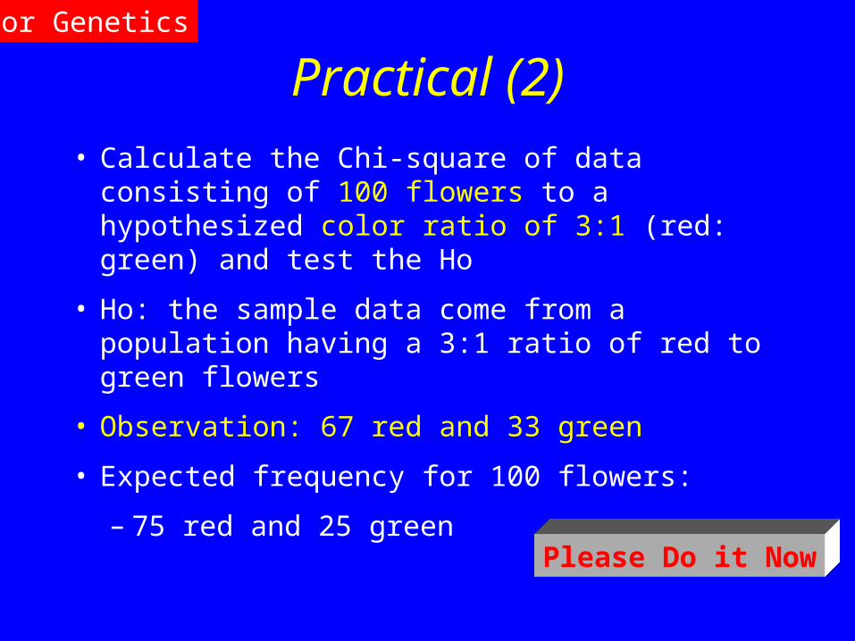
Practical (2)
• Calculate the Chi-square of data consisting of 100 flowers to a hypothesized color ratio of 3:1 (red: green) and test the Ho
• Ho: the sample data come from a population having a 3:1 ratio of red to green flowers
• Observation: 67 red and 33 green
• Expected frequency for 100 flowers:
– 75 red and 25 green Please Do it Now
For Genetics
For > 2 categories
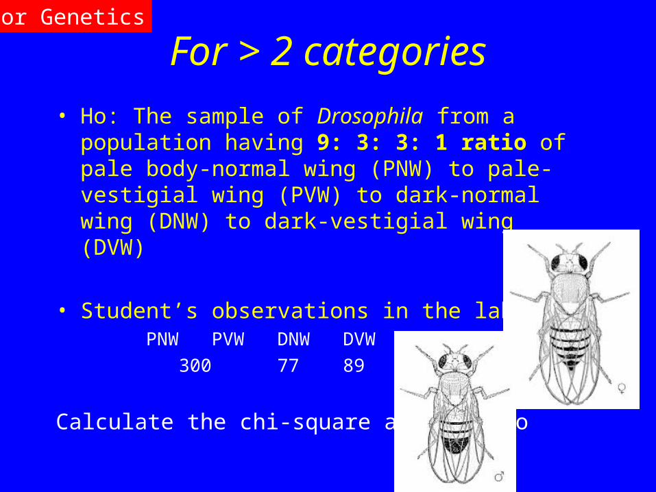
• Ho: The sample of Drosophila from a population having 9: 3: 3: 1 ratio of pale body-normal wing (PNW) to pale-vestigial wing (PVW) to dark-normal wing (DNW) to dark-vestigial wing (DVW)
• Student’s observations in the lab: PNW PVW DNW DVW Total
300 77 89 36 502
Calculate the chi-square and test Ho
For Genetics
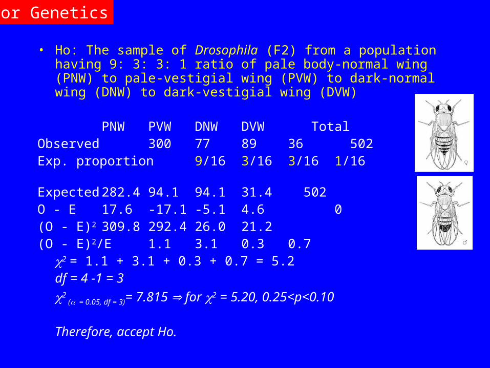
• Ho: The sample of Drosophila (F2) from a population having 9: 3: 3: 1 ratio of pale body-normal wing (PNW) to pale-vestigial wing (PVW) to dark-normal wing (DNW) to dark-vestigial wing (DVW)
PNW PVW DNW DVW TotalObserved 300 77 89 36 502Exp. proportion 9/16 3/16 3/16 1/16 1Expected 282.4 94.1 94.1 31.4 502O - E 17.6 -17.1 -5.1 4.6 0(O - E)2 309.8 292.4 26.0 21.2(O - E)2/E 1.1 3.1 0.3 0.7
2 = 1.1 + 3.1 + 0.3 + 0.7 = 5.2df = 4 -1 = 3
2 ( = 0.05, df = 3)= 7.815 for 2 = 5.20, 0.25<p<0.10
Therefore, accept Ho.
For Genetics
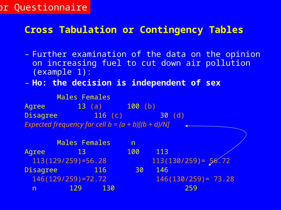
Cross Tabulation or Contingency Tables
– Further examination of the data on the opinion on increasing fuel to cut down air pollution (example 1):
– Ho: the decision is independent of sex
Males FemalesAgree 13 (a) 100 (b)Disagree 116 (c) 30 (d)Expected frequency for cell b = (a + b)[(b + d)/N]
Males Females nAgree 13 100 113
113(129/259)=56.28 113(130/259)= 56.72Disagree 116 30 146
146(129/259)=72.72 146(130/259)= 73.28n 129 130 259
For Questionnaire
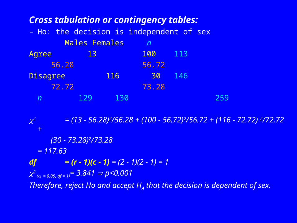
Cross tabulation or contingency tables:– Ho: the decision is independent of sex
Males Females n
Agree 13 100 113
56.28 56.72
Disagree 116 30 146
72.72 73.28
n 129 130 259
2 = (13 - 56.28)2/56.28 + (100 - 56.72)2/56.72 + (116 - 72.72) 2/72.72 +
(30 - 73.28)2/73.28
= 117.63
df = (r - 1)(c - 1) = (2 - 1)(2 - 1) = 1
2 ( = 0.05, df = 1)= 3.841 p<0.001
Therefore, reject Ho and accept HA that the decision is dependent of sex.

Quicker method for 2 x 2 cross tabulation:Class A Class B n
State 1 a b a + bState 2 c d c + d
n a + c b + d n = a + b + c +d2 = n (ad - bc)2/(a + b)(c + d)(a + c)(b + d)
Males FemalesAgree 13 100 113Disagree 116 30 146
129 130 2592 = 259(13 30 - 116 100)2/(113)(146)(129)(130) =
117.64
2 ( = 0.05, df = 1)= 3.841 p<0.001; Therefore, rejected Ho.
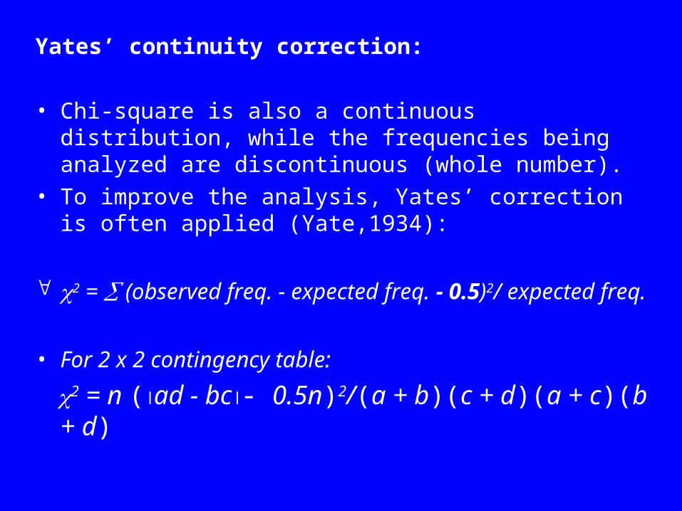
Yates’ continuity correction:
• Chi-square is also a continuous distribution, while the frequencies being analyzed are discontinuous (whole number).
• To improve the analysis, Yates’ correction is often applied (Yate,1934):
2 = (observed freq. - expected freq. - 0.5)2/ expected freq.
• For 2 x 2 contingency table:
2 = n (ad - bc- 0.5n)2/(a + b)(c + d)(a + c)(b + d)

Yates’ Correction (example 1):
2 = n (ad - bc- 0.5n)2/(a + b)(c + d)(a + c)(b + d)
Males Females
Agree 13 100 113
Disagree 116 30 146
129 130 259
2 = 259(1330 - 116100 -0.5259)2/(113)(146)(129)(130)
= 114.935 (smaller than 117.64, less bias)
2 ( = 0.05, df = 1)= 3.841 p<0.001; Therefore, rejected Ho.

Practical 3: 2 = n (ad - bc- 0.5n)2/(a + b)(c + d)(a + c)(b +
d)• For a drug test, Ho: The survival of the animals is
independent of whether the drug is administered
Dead Alive n
Treated 12 30 42
Not treated 27 31 58
n 39 61 100
Using Yates’ correction to calculate 2 and test the hypothesis
Please do it at home

Bias in Chi-square calculations
• If values of expected frequency (fi) are very small, the calculated 2 is biased in that it is larger than the theoretical 2 value and we shall tend to reject Ho.
• Rules: fi > 1 and no more than 20% of fi < 5.0.
• It may be conservative at significance levels < 5%, especially when the expected frequencies are all equal.
• If having small fi, (1) increase the sample size if possible, use G-test or (2) combine the categories if possible.

The G test (log-likelihood ratio)G = 2 O ln (O/E)
• Similar to the 2 test
• Many statisticians believe that the G test is superior to the 2 test (although at present it is not as popular)
• For 2 x 2 cross tabulation:
Class A Class B
State 1 a b
State 2 c dThe expected frequency for cell a = (a+b)[(a+c)/n]
Practical 3 Dead Alive n
Treated 12 (16.38) 30 (25.62) 42
Not treated 27 (22.62) 31 (35.38) 58
n 39 61 100
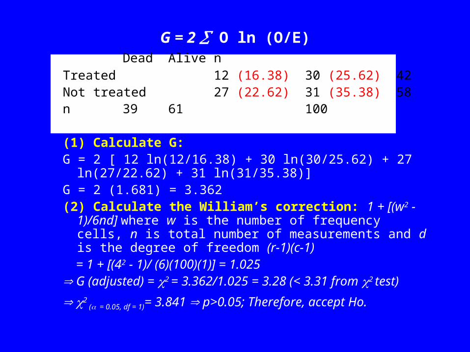
G = 2 O ln (O/E) Dead Alive n
Treated 12 (16.38) 30 (25.62) 42Not treated 27 (22.62) 31 (35.38) 58n 39 61 100
(1) Calculate G:G = 2 [ 12 ln(12/16.38) + 30 ln(30/25.62) + 27 ln(27/22.62) + 31
ln(31/35.38)]G = 2 (1.681) = 3.362(2) Calculate the William’s correction: 1 + [(w2 - 1)/6nd] where w
is the number of frequency cells, n is total number of measurements and d is the degree of freedom (r-1)(c-1)
= 1 + [(42 - 1)/ (6)(100)(1)] = 1.025 G (adjusted) = 2 = 3.362/1.025 = 3.28 (< 3.31 from 2 test)
2 ( = 0.05, df = 1)= 3.841 p>0.05; Therefore, accept Ho.

• Ho: The sample of Drosophila (F2) from a population having 9: 3: 3: 1 ratio of pale body-normal wing (PNW) to pale-vestigial wing (PVW) to dark-normal wing (DNW) to dark-vestigial wing (DVW)
PNW PVW DNW DVW Total
Observed 300 77 89 36 502
Expected 282.4 94.1 94.1 31.4
O ln(O/E) 18.14 -15.44 -4.96 4.92
G value: G = 2 (18.14 - 15.44 - 4.96 + 4.92) = 5.32
William’s correction: 1 + [(42 - 1)/6 (502) (3)] = 1.00166
G (adjusted): 5.32/1.00166 = 5.311
2 ( = 0.05, df = 3)= 7.815 for 2 = 5.20, 0.25<p<0.10
Therefore, accept Ho.
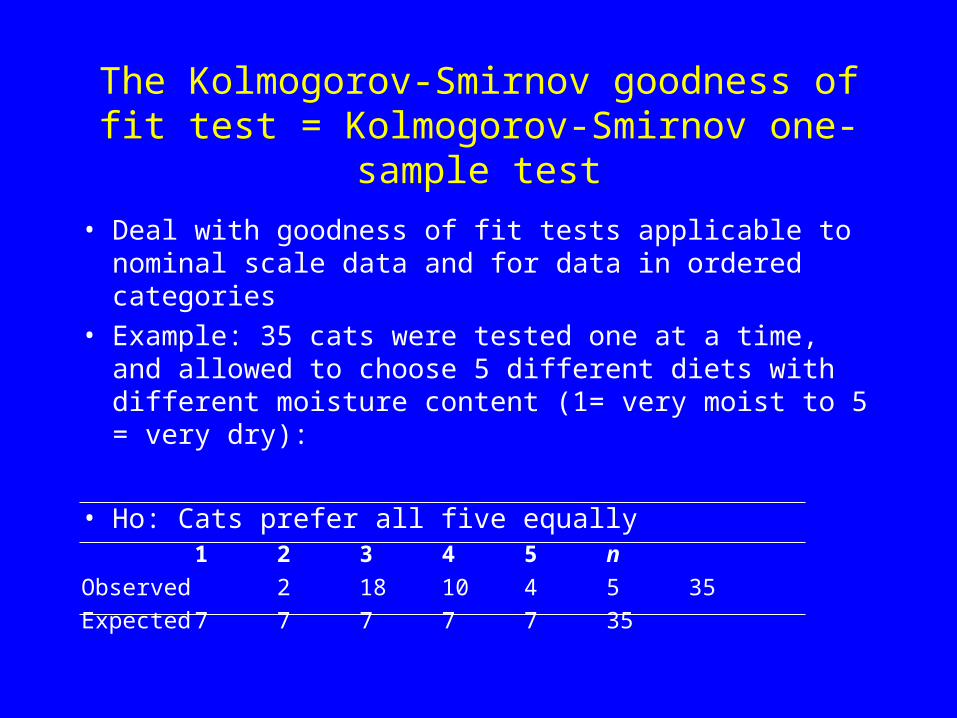
The Kolmogorov-Smirnov goodness of fit test = Kolmogorov-Smirnov one-sample test
• Deal with goodness of fit tests applicable to nominal scale data and for data in ordered categories
• Example: 35 cats were tested one at a time, and allowed to choose 5 different diets with different moisture content (1= very moist to 5 = very dry):
• Ho: Cats prefer all five equally 1 2 3 4 5 n
Observed 2 18 10 4 5 35
Expected 7 7 7 7 7 35
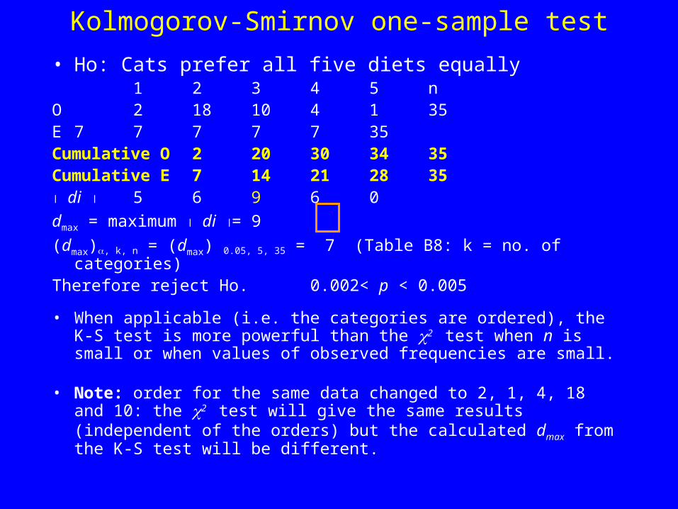
Kolmogorov-Smirnov one-sample test
• Ho: Cats prefer all five diets equally 1 2 3 4 5 n
O 2 18 10 4 1 35E 7 7 7 7 7 35Cumulative O 2 20 30 34 35Cumulative E 7 14 21 28 35 di 5 6 9 6 0
dmax = maximum di = 9
(dmax), k, n = (dmax) 0.05, 5, 35 = 7 (Table B8: k = no. of categories) Therefore reject Ho. 0.002< p < 0.005
• When applicable (i.e. the categories are ordered), the K-S test is more powerful than the 2 test when n is small or when values of observed frequencies are small.
• Note: order for the same data changed to 2, 1, 4, 18 and 10: the 2 test will give the same results (independent of the orders) but the calculated dmax from the K-S test will be different.
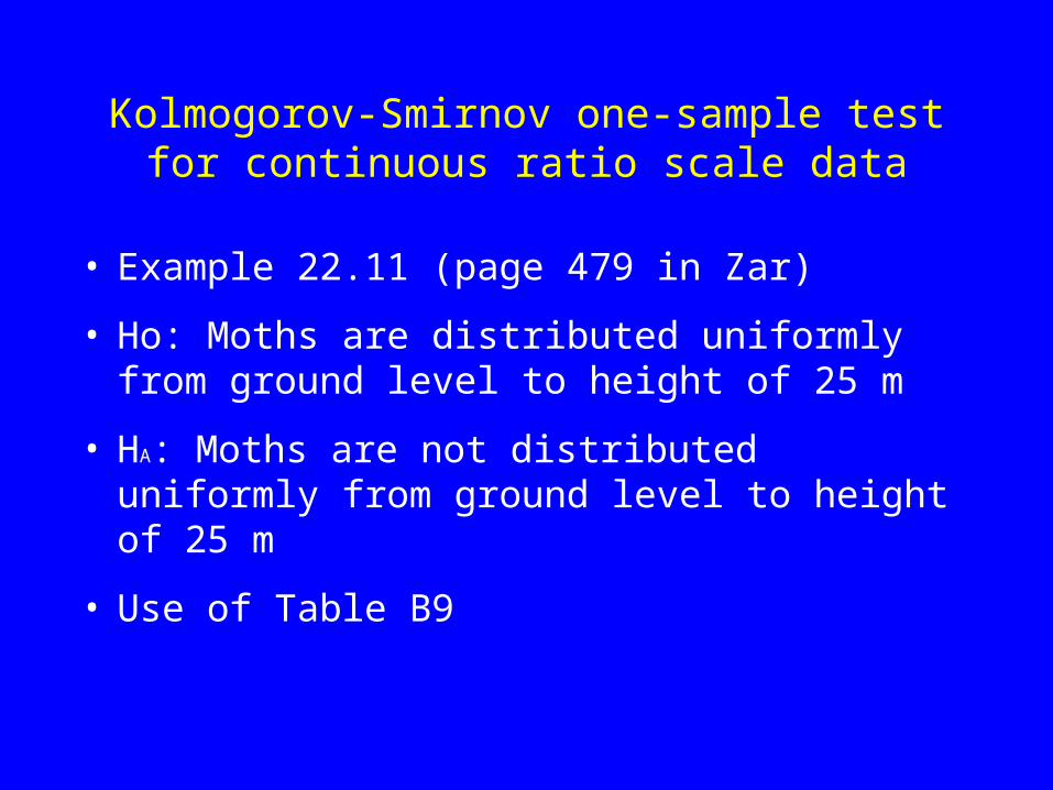
Kolmogorov-Smirnov one-sample test for continuous ratio scale data
• Example 22.11 (page 479 in Zar)
• Ho: Moths are distributed uniformly from ground level to height of 25 m
• HA: Moths are not distributed uniformly from ground level to height of 25 m
• Use of Table B9
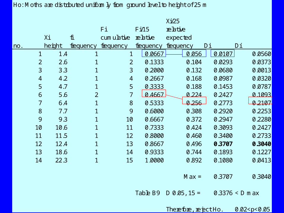
Ho: Moths are distributed uniformly from ground level to height of 25 m
Xi/25Fi Fi/15 relative
Xi fi cumulative relative expectedno. height frequency frequency frequency frequency Di Dí
1 1.4 1 1 0.0667 0.056 0.0107 0.05602 2.6 1 2 0.1333 0.104 0.0293 0.03733 3.3 1 3 0.2000 0.132 0.0680 0.00134 4.2 1 4 0.2667 0.168 0.0987 0.03205 4.7 1 5 0.3333 0.188 0.1453 0.07876 5.6 2 7 0.4667 0.224 0.2427 0.10937 6.4 1 8 0.5333 0.256 0.2773 0.21078 7.7 1 9 0.6000 0.308 0.2920 0.22539 9.3 1 10 0.6667 0.372 0.2947 0.2280
10 10.6 1 11 0.7333 0.424 0.3093 0.242711 11.5 1 12 0.8000 0.460 0.3400 0.273312 12.4 1 13 0.8667 0.496 0.3707 0.304013 18.6 1 14 0.9333 0.744 0.1893 0.122714 22.3 1 15 1.0000 0.892 0.1080 0.0413
Max = 0.3707 0.3040
Table B9 D 0.05, 15 = 0.3376 < D max
Therefore, reject Ho. 0.02<p<0.05
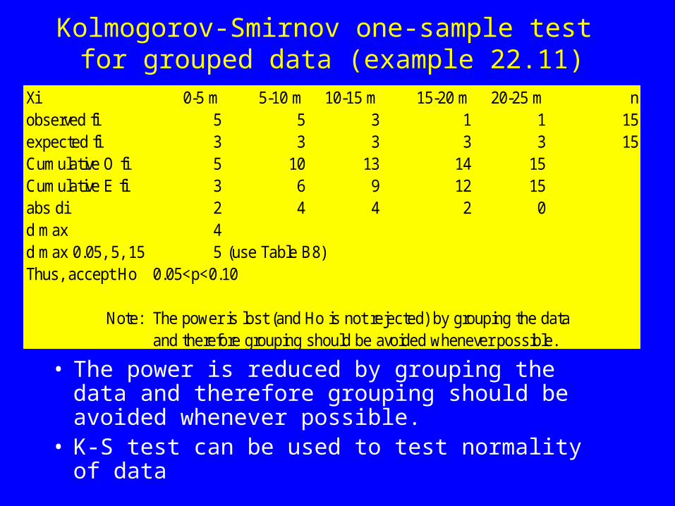
Kolmogorov-Smirnov one-sample test for grouped data (example 22.11)
• The power is reduced by grouping the data and therefore grouping should be avoided whenever possible.
• K-S test can be used to test normality of data
Xi 0-5 m 5-10 m 10-15 m 15-20 m 20-25 m nobserved fi 5 5 3 1 1 15expected fi 3 3 3 3 3 15Cumulative O fi 5 10 13 14 15Cumulative E fi 3 6 9 12 15abs di 2 4 4 2 0d max 4d max 0.05, 5, 15 5 (use Table B8)Thus, accept Ho 0.05<p<0.10
Note: The power is lost (and Ho is not rejected) by grouping the data and therefore grouping should be avoided whenever possible.

• Recognizing the distribution of your data is important – Provides a firm base on which to establish
and test hypotheses
– If data are normally distributed, you can use parametric tests;
– Otherwise transform data to normal distribution
– Or non-parametric tests should be performed
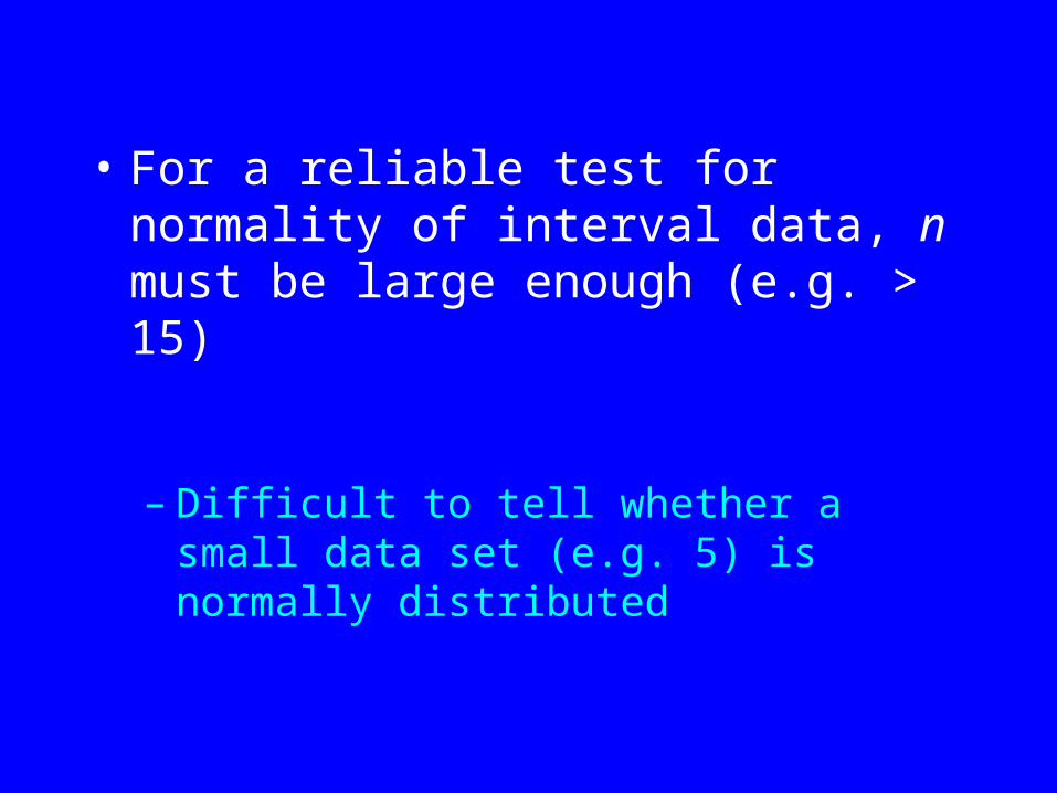
• For a reliable test for normality of interval data, n must be large enough (e.g. > 15)
– Difficult to tell whether a small data set (e.g. 5) is normally distributed

• Inspection of the frequency histogram
• Probability plot
• Chi-square goodness of fit
• Kolmogorov-Smirnov one-sample test
• Symmetry and Kurtosis: D’Agostino-Pearson K2 test (Chapters 6 & 7, Zar 99)
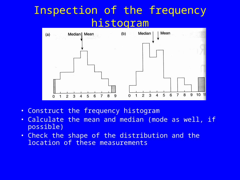
Inspection of the frequency histogram
• Construct the frequency histogram• Calculate the mean and median (mode as well, if possible)• Check the shape of the distribution and the location of
these measurements
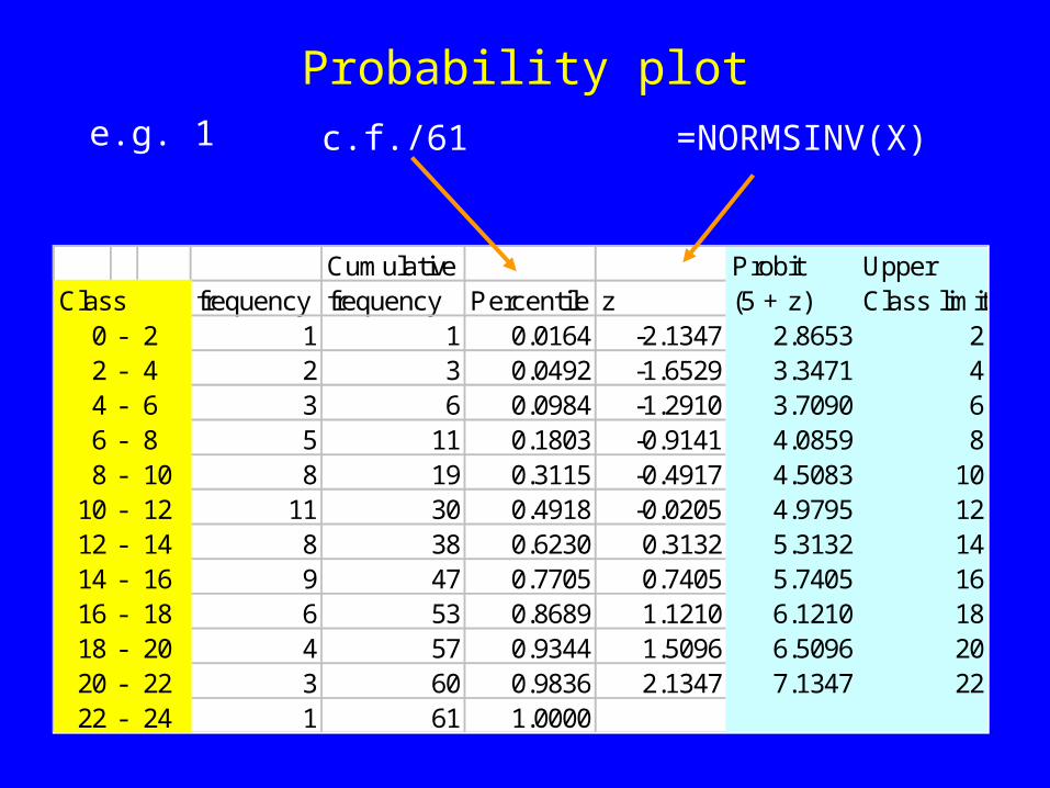
Probability plote.g. 1
Cumulative Probit UpperClass frequency frequency Percentile z (5 + z) Class limit
0 - 2 1 1 0.0164 -2.1347 2.8653 22 - 4 2 3 0.0492 -1.6529 3.3471 44 - 6 3 6 0.0984 -1.2910 3.7090 66 - 8 5 11 0.1803 -0.9141 4.0859 88 - 10 8 19 0.3115 -0.4917 4.5083 10
10 - 12 11 30 0.4918 -0.0205 4.9795 1212 - 14 8 38 0.6230 0.3132 5.3132 1414 - 16 9 47 0.7705 0.7405 5.7405 1616 - 18 6 53 0.8689 1.1210 6.1210 1818 - 20 4 57 0.9344 1.5096 6.5096 2020 - 22 3 60 0.9836 2.1347 7.1347 2222 - 24 1 61 1.0000
=NORMSINV(X)c.f./61

0
2
4
6
8
10
12
1 2 3 4 5 6 7 8 9 10 11 12
Bin number (bin size = 2)
fre
qu
en
cy
Probability plot
y = 0.8502x + 0.0736R2 = 0.9711
0.0
0.1
0.2
0.3
0.4
0.5
0.6
0.7
0.8
0.9
1.0
0.0 0.2 0.4 0.6 0.8 1.0
Observed cumulative p
Exp
ect
ed
cu
mu
lati
ve p
e.g. 1
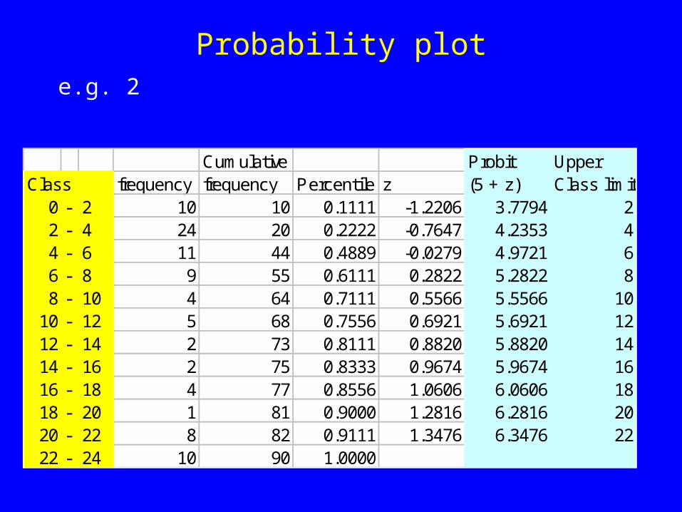
Cumulative Probit UpperClass frequency frequency Percentile z (5 + z) Class limit
0 - 2 10 10 0.1111 -1.2206 3.7794 22 - 4 24 20 0.2222 -0.7647 4.2353 44 - 6 11 44 0.4889 -0.0279 4.9721 66 - 8 9 55 0.6111 0.2822 5.2822 88 - 10 4 64 0.7111 0.5566 5.5566 10
10 - 12 5 68 0.7556 0.6921 5.6921 1212 - 14 2 73 0.8111 0.8820 5.8820 1414 - 16 2 75 0.8333 0.9674 5.9674 1616 - 18 4 77 0.8556 1.0606 6.0606 1818 - 20 1 81 0.9000 1.2816 6.2816 2020 - 22 8 82 0.9111 1.3476 6.3476 2222 - 24 10 90 1.0000
Probability plote.g. 2

• Obviously, the data is not distributed on the line.
• Based on the frequency distribution of the data, the distribution is positive skew (higher frequencies at lower classes)
0
5
10
15
20
25
30
1 2 3 4 5 6 7 8 9 10 11 12
Bin number (bin size = 2)
Fre
qu
en
cy
Probability plote.g. 2
y = 1.0876x - 0.2443R2 = 0.8576
0.0
0.1
0.2
0.3
0.4
0.5
0.6
0.7
0.8
0.9
1.0
0.0 0.2 0.4 0.6 0.8 1.0
Obs cum P
Exp
cu
m P

• Concave curve indicates positive skew which suggest a log-normal distribution (i.e. log-transformation of the upper class limit is required)
very common e.g. mortality rates
• Convex curve indicates negative skew less common (e.g. some binomial distribution)

• Bimodal distributions e.g. toxicity data produce a sigmoid probability plot
• Multi-modal distributions: data from animals with several age-classes; undulating wave-like curve
• S-shaped curve suggests ‘bad’ kurtosis: Normality departure but their mean, median, mode remain equal
• Leptokurtic distribution: data bunched around the mean, giving a sharp peak
• Platykurtic distribution: a board summit which falls rapidly in the tails
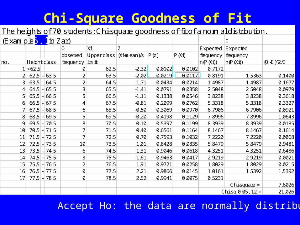
The heights of 70 students: Chi-square goodness of fit of a normal distribution.(Example 7.4 in Zar) E
O Xi Z Expected Expected observed Upper class (Xi-mean)/s P(z) P(Xi) frequency frequency
no. Height class frequency limit n(P(Xi)) n(P(Xi)) (O-E) 2̂/E1 <62.5 0 62.5 -2.32 0.0102 0.0102 0.71722 62.5 - 63.5 2 63.5 -2.02 0.0219 0.0117 0.8191 1.5363 0.14003 63.5 - 64.5 2 64.5 -1.71 0.0434 0.0214 1.4987 1.4987 0.16774 64.5 - 65.5 3 65.5 -1.41 0.0791 0.0358 2.5048 2.5048 0.09795 65.5 - 66.5 5 66.5 -1.11 0.1338 0.0546 3.8238 3.8238 0.36186 66.5 - 67.5 4 67.5 -0.81 0.2099 0.0762 5.3318 5.3318 0.33277 67.5 - 68.5 6 68.5 -0.50 0.3069 0.0970 6.7906 6.7906 0.09218 68.5 - 69.5 5 69.5 -0.20 0.4198 0.1129 7.8996 7.8996 1.06439 69.5 - 70.5 8 70.5 0.10 0.5397 0.1199 8.3939 8.3939 0.0185
10 70.5 - 71.5 7 71.5 0.40 0.6561 0.1164 8.1467 8.1467 0.161411 71.5 - 72.5 7 72.5 0.70 0.7593 0.1032 7.2220 7.2220 0.006812 72.5 - 73.5 10 73.5 1.01 0.8428 0.0835 5.8479 5.8479 2.948113 73.5 - 74.5 6 74.5 1.31 0.9046 0.0618 4.3251 4.3251 0.648614 74.5 - 75.5 3 75.5 1.61 0.9463 0.0417 2.9219 2.9219 0.002115 75.5 - 76.5 2 76.5 1.91 0.9721 0.0258 1.8029 1.8029 0.021516 76.5 - 77.5 0 77.5 2.21 0.9866 0.0145 1.0161 1.5392 1.539217 77.5 - 78.5 0 78.5 2.52 0.9941 0.0075 0.5231
Chi-square = 7.6026Chi-sq 0.05, 12 = 21.026
Chi-Square Goodness of Fit
Accept Ho: the data are normally distributed
6.1

Xi fi fiXi fi(Xi) 2̂Mid height freq
63 2 126 793864 2 128 819265 3 195 1267566 5 330 2178067 4 268 1795668 6 408 2774469 5 345 2380570 8 560 3920071 7 497 3528772 7 504 3628873 10 730 5329074 6 444 3285675 3 225 1687576 2 152 11552
sum 70 4912 345438
mean 70.17sd 3.310
0
2
4
6
8
10
12
60 65 70 75 80
Height (in), Xi
Fre
qu
en
cy
Observed
Expected
=(345438-(49122/70))/(70-1)
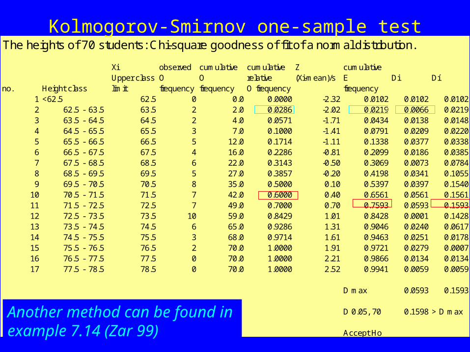
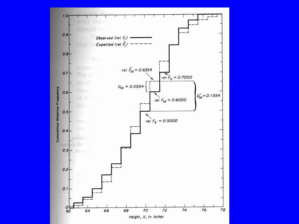
The heights of 70 students: Chi-square goodness of fit of a normal distribution.
Xi observed cumulative cumulative Z cumulative Upper class O O relative (Xi-mean)/s E Di Dí
no. Height class limit frequency frequency O frequency frequency1 <62.5 62.5 0 0.0 0.0000 -2.32 0.0102 0.0102 0.01022 62.5 - 63.5 63.5 2 2.0 0.0286 -2.02 0.0219 0.0066 0.02193 63.5 - 64.5 64.5 2 4.0 0.0571 -1.71 0.0434 0.0138 0.01484 64.5 - 65.5 65.5 3 7.0 0.1000 -1.41 0.0791 0.0209 0.02205 65.5 - 66.5 66.5 5 12.0 0.1714 -1.11 0.1338 0.0377 0.03386 66.5 - 67.5 67.5 4 16.0 0.2286 -0.81 0.2099 0.0186 0.03857 67.5 - 68.5 68.5 6 22.0 0.3143 -0.50 0.3069 0.0073 0.07848 68.5 - 69.5 69.5 5 27.0 0.3857 -0.20 0.4198 0.0341 0.10559 69.5 - 70.5 70.5 8 35.0 0.5000 0.10 0.5397 0.0397 0.1540
10 70.5 - 71.5 71.5 7 42.0 0.6000 0.40 0.6561 0.0561 0.156111 71.5 - 72.5 72.5 7 49.0 0.7000 0.70 0.7593 0.0593 0.159312 72.5 - 73.5 73.5 10 59.0 0.8429 1.01 0.8428 0.0001 0.142813 73.5 - 74.5 74.5 6 65.0 0.9286 1.31 0.9046 0.0240 0.061714 74.5 - 75.5 75.5 3 68.0 0.9714 1.61 0.9463 0.0251 0.017815 75.5 - 76.5 76.5 2 70.0 1.0000 1.91 0.9721 0.0279 0.000716 76.5 - 77.5 77.5 0 70.0 1.0000 2.21 0.9866 0.0134 0.013417 77.5 - 78.5 78.5 0 70.0 1.0000 2.52 0.9941 0.0059 0.0059
D max 0.0593 0.1593
D 0.05, 70 0.1598 > D max
Accept Ho
Kolmogorov-Smirnov one-sample test
Another method can be found in example 7.14 (Zar 99)

Symmetry (Skewness) and Kurtosis
Skewness
• A measure of the asymmetry of a distribution.
• The normal distribution is symmetric, and has a skewness value of zero.
• A distribution with a significant positive skewness has a long right tail.
• A distribution with a significant negative skewness has a long left tail.
• As a rough guide, a skewness value more than twice it's standard error is taken to indicate a departure from symmetry.

Symmetry (Skewness) and Kurtosis
Kurtosis
• A measure of the extent to which observations cluster around a central point.
• For a normal distribution, the value of the kurtosis statistic is 0.
• Positive kurtosis indicates that the observations cluster more and have longer tails than those in the normal distribution ( leptokurtic).
• Negative kurtosis indicates the observations cluster less and have shorter tails ( Platykurtic).

• You should read the Chapters 1-7 of Zar 1999 which have been covered by the five lectures so far.
• The frequency distribution of a sample can often be identified with a theoretical distribution, such as the normal distribution.
• Five methods for comparing a sample distribution: inspection of the frequency histogram; probability plot; Chi-square goodness of fit, Kolmogorov-Smirnov one-sample test and D’Agostino-Pearson K2 test.
• Probability plots can be used for testing normal and log-normal distributions.
• Graphical methods often provide evidence of non-normal distributions, such as skewness and kurtosis (Excel or SPSS can determine the degree of these two measurements).
• The Chi-square goodness of fit or Kolmogorov-Smirnov one-sample test also can be used to test of an unknown distribution against a theoretical distribution (apart from normal distribution).
Binomial & Poisson Distributions
and their Application
(Chapters 24 & 25, Zar 1999)
Binomial
• Consider nominal scale data that come from a population with only two categories
– members of a mammal litter may be classified as male or female
– victims of an epidemic as dead or alive
– progeny of a Drosophila cross as white-eyed or red-eyed

Binomial Distributions
The proportion of the population belonging to one of the two categories is denoted as:
– p, then the other q = 1- p
– e.g. if 48% male and 52% female so
p = 0.48 and q = 0.52

(Source of photos: BBC)
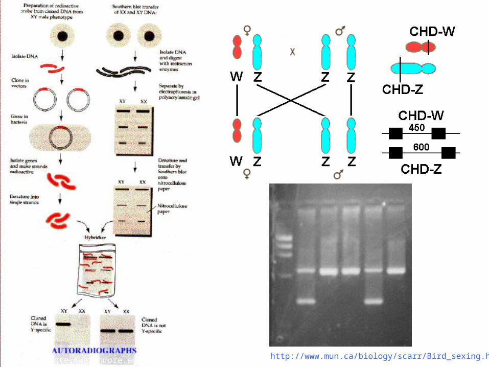
http://www.mun.ca/biology/scarr/Bird_sexing.htmhttp://zygote.swarthmore.edu/chap20.html

Binomial Distributions
• e.g. if p = 0.4 and q = 0.6: for taking 10 random samples, you will expect 4 males and 6 females; however, you might get 1 male and 9 females.
• The probabilities of two independent events both occurring is the product of the probabilities of the two separate events:
– (p)(q) = (0.4)(0.6) = 0.24;
– (p)(p) = 0.16; and
– (q)(q) = 0.36

Binomial Distributions
• e.g. if p = 0.4 and q = 0.6: for taking 10 random samples, you will expect 4 males and 6 females
• The probabilities of either of two independent events is sum of the probabilities of each event, e.g. for having one male and one female in the sample:
pq + qp = 2 pq = 2(0.4)(0.6) = 0.48
• For having all male, all female,
Both sexes = 0.16 + 0.36 + 0.48 = 1

Binomial Distributions
If a random sample of size n is taken from a binomial population, the probability of X individuals being in one category (other category = n - X) is
P(X) = [(n!)/(X!(n-X)!)](pX)(qn-X)
For n = 5, X = 3, p = q = 0.5, then P(X) = (5!/3!2!)(0.53)(0.52)P(X) = (10)(0.125)(0.25) = 0.3125
For X = 0, 1, 2 , 4, 5, P(X) = 0.03125, 0.15625, 0.31250, 0.15625, 0.03125, respectively
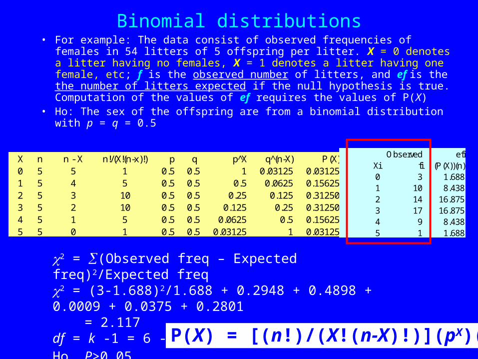
Binomial distributions• For example: The data consist of observed frequencies of females in 54
litters of 5 offspring per litter. X = 0 denotes a litter having no females, X = 1 denotes a litter having one female, etc; f is the observed number of litters, and ef is the the number of litters expected if the null hypothesis is true. Computation of the values of ef requires the values of P(X)
• Ho: The sex of the offspring are from a binomial distribution with p = q = 0.5
X n n - X n!/(X!(n-x)!) p q p^X q (̂n-X) P(X)0 5 5 1 0.5 0.5 1 0.03125 0.031251 5 4 5 0.5 0.5 0.5 0.0625 0.156252 5 3 10 0.5 0.5 0.25 0.125 0.312503 5 2 10 0.5 0.5 0.125 0.25 0.312504 5 1 5 0.5 0.5 0.0625 0.5 0.156255 5 0 1 0.5 0.5 0.03125 1 0.03125
Observed efiXi fi (P(X))(n)0 3 1.6881 10 8.4382 14 16.8753 17 16.8754 9 8.4385 1 1.688
2 = (Observed freq – Expected freq)2/Expected freq 2 = (3-1.688)2/1.688 + 0.2948 + 0.4898 + 0.0009 + 0.0375 + 0.2801 = 2.117df = k -1 = 6 -1 = 5; 2 0.05, 5 = 11.07 so accept Ho. P>0.05
P(X) = [(n!)/(X!(n-X)!)](pX)(qn-X)
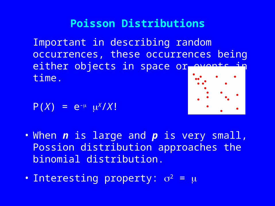
Poisson Distributions
Important in describing random occurrences, these occurrences being either objects in space or events in time.
P(X) = e- X/X!
• When n is large and p is very small, Possion distribution approaches the binomial distribution.
• Interesting property: 2 =

Poisson Distributions
P(X) = e- X/X! • e.g. The data are the number of sparrow nests in an
area of given size (8,000 m2). There are totally 40 areas of the same size surveyed. Then Xi is the number of nests in an area; fi is the frequency of Xi nests per hectare; and P(Xi) is the probability of Xi nests per hectare, if the nests are distributed randomly.
• Ho: the population of sparrow nests is distributed randomly
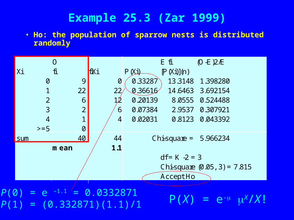
Example 25.3 (Zar 1999)
• Ho: the population of sparrow nests is distributed randomly
O E fi (O-E)2/EXi fi fiXi P(Xi) [P(Xi)](n)
0 9 0 0.33287 13.3148 1.3982801 22 22 0.36616 14.6463 3.6921542 6 12 0.20139 8.0555 0.5244883 2 6 0.07384 2.9537 0.3079214 1 4 0.02031 0.8123 0.043392
>=5 0sum 40 44 Chi-square = 5.966234
mean 1.1df = K -2 = 3Chi-square (0.05, 3) = 7.815Accept Ho
P(0) = e –1.1 = 0.0332871P(1) = (0.332871)(1.1)/1 P(X) = e- X/X!

For further reading on Binomial and Poisson distributions: Zar’s chapters 24 and 25


