E&CE 380 Frequency Response AnalysisE&CE 380 Frequency Response Analysis
Frequency Response MethodsFrequency Response MethodsStability AnalysisStability Analysis
• The Nyquist plot provides absolute and The Nyquist plot provides absolute and relative relative stabilitystability information about the information about the closed-loopclosed-loop system, based on a plot of the system, based on a plot of the loop loop characteristicscharacteristics of the system. of the system.
• The most important section of the Nyquist plot The most important section of the Nyquist plot corresponds to corresponds to section IIsection II of the Nyquist path, of the Nyquist path, ss = = jj, with , with = 0 = 0++
• This corresponds to the This corresponds to the frequency responsefrequency response characteristics of the characteristics of the looploop transfer function. transfer function.
E&CE 380 Frequency Response AnalysisE&CE 380 Frequency Response Analysis
Frequency Response MethodsFrequency Response MethodsStability AnalysisStability Analysis
• In the In the Nyquist plotNyquist plot, this information is plotted in , this information is plotted in polar form, magnitude and phase angle as frequency polar form, magnitude and phase angle as frequency is varied.is varied.
• This same information can be plotted in two This same information can be plotted in two rectangular plots of rectangular plots of magnitudemagnitude (in (in dBdB) vs. frequency ) vs. frequency and and phase anglephase angle vs. frequency ( vs. frequency (Bode plotsBode plots).).
• The same Nyquist The same Nyquist relative stability criteriarelative stability criteria can be can be interpreted in terms of these rectangular plots interpreted in terms of these rectangular plots
E&CE 380 Frequency Response AnalysisE&CE 380 Frequency Response Analysis
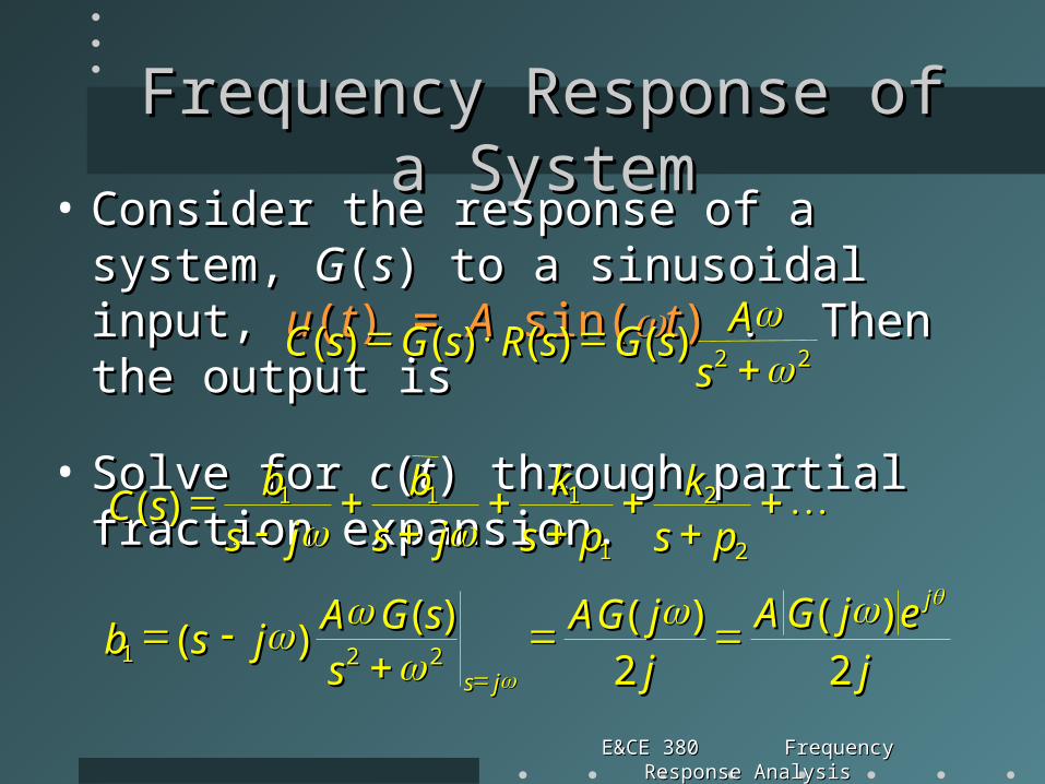
Frequency Response of a SystemFrequency Response of a System• Consider the response of a system, Consider the response of a system, GG((ss) to a ) to a
sinusoidal input, sinusoidal input, uu((tt) = ) = AA sin( sin(tt)) . Then the . Then the output isoutput is
• Solve for Solve for cc((tt) through partial fraction ) through partial fraction expansion.expansion.
2222))(())(())(())((
ss
AAssGGssRRssGGssCC
jjeejjGGAA
jjjjGGAA
ssssGGAA
jjssbbjj
jjss 22))((
22))(())((
))(( 222211
ppsskk
ppsskk
jjssbb
jjssbb
ssCC ))((22
22
11
111111
E&CE 380 Frequency Response AnalysisE&CE 380 Frequency Response Analysis
Frequency Response of a SystemFrequency Response of a System
))((// jjGG
22))((
22))(())((
))(( 222211
jjeejjGGAA
jjjjGGAA
ssssGGAA
jjssbbjj
jjss
wherewhere
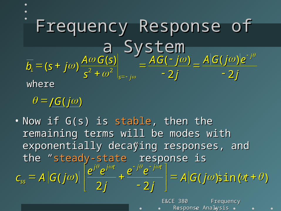
• Now if G(s) is Now if G(s) is stablestable, then the remaining terms , then the remaining terms will be modes with exponentially decaying will be modes with exponentially decaying responses, and the “responses, and the “steady-statesteady-state” response is” response is
))sin(sin())((2222
))((
ttjjGGAAjj
eeee
jjeeee
jjGGAAccttjjjjttjjjj
ssss
E&CE 380 Frequency Response AnalysisE&CE 380 Frequency Response Analysis
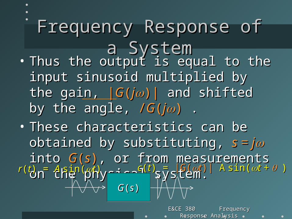
Frequency Response of a SystemFrequency Response of a System• Thus the output is equal to the input sinusoid Thus the output is equal to the input sinusoid
multiplied by the gain, multiplied by the gain, ||GG((jj)|)| and shifted by and shifted by the angle, the angle, //GG((jj)) . .
• These characteristics can be obtained by These characteristics can be obtained by substituting, substituting, s = js = j into into GG((ss)), or from , or from measurements on the physical system.measurements on the physical system.
GG((ss))GG((ss))
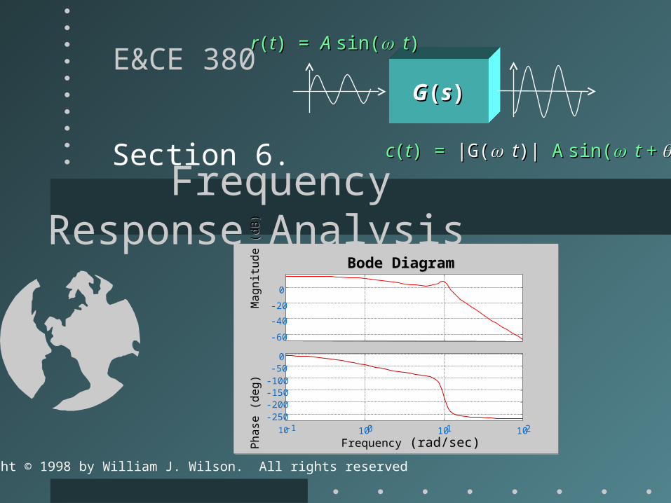
rr((tt) = ) = A A sin(sin(tt)) cc((tt) =) = |G(|G(tt)|)| AA sin(sin(t +t + ))
E&CE 380 Frequency Response AnalysisE&CE 380 Frequency Response Analysis
Frequency Response AnalysisFrequency Response AnalysisBode PlotsBode Plots
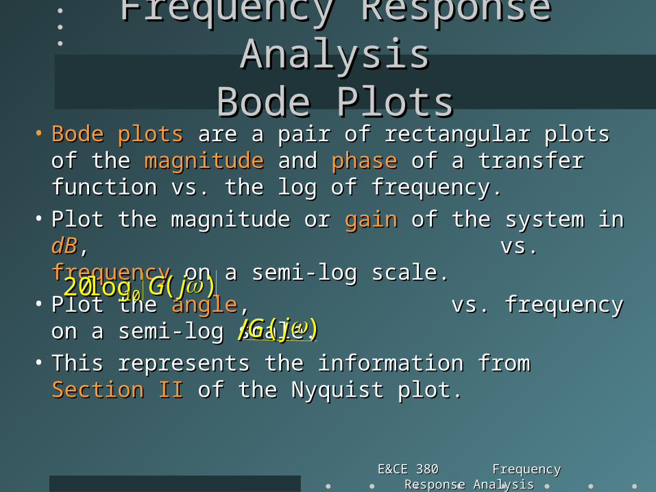
• Bode plotsBode plots are a pair of rectangular plots of the are a pair of rectangular plots of the magnitudemagnitude and and phasephase of a transfer function vs. the log of of a transfer function vs. the log of frequency.frequency.
• Plot the magnitude or Plot the magnitude or gaingain of the system in of the system in dBdB, , vs. vs. frequencyfrequency on a semi-log scale. on a semi-log scale.
• Plot the Plot the angleangle, vs. frequency on a semi-log , vs. frequency on a semi-log scale.scale.
• This represents the information from This represents the information from Section IISection II of the of the Nyquist plot.Nyquist plot.
))((loglog2020 1010 jjGG
))((// jjGG
E&CE 380 Frequency Response AnalysisE&CE 380 Frequency Response Analysis
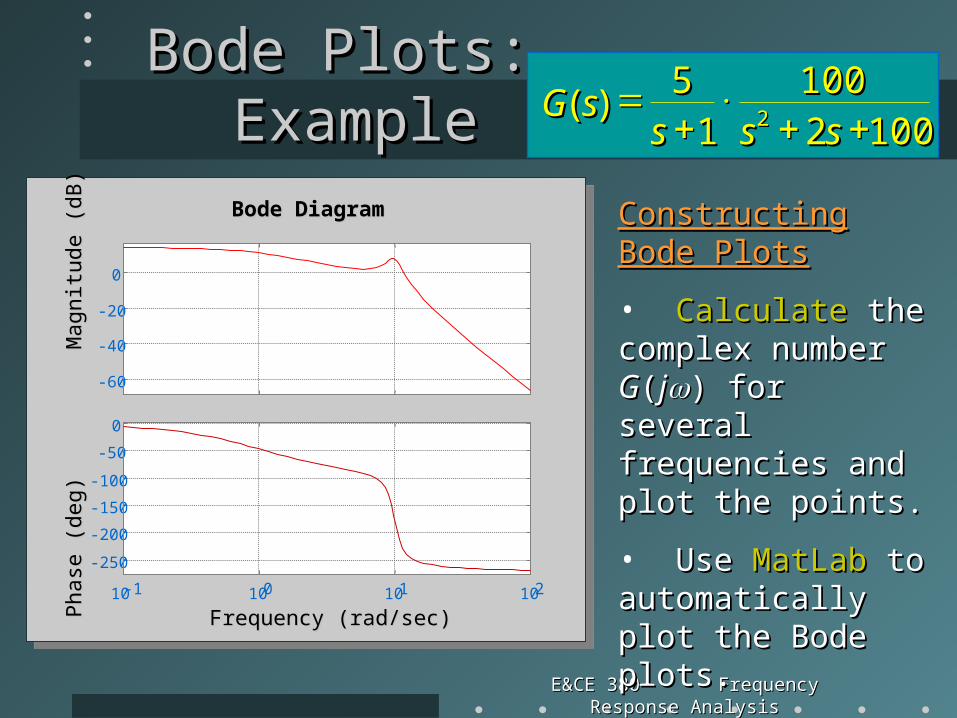
Bode Plots:Bode Plots: Example Example
Frequency (rad/sec)Frequency (rad/sec)
Pha
se (
deg)
M
agni
tude
(dB
)P
hase
(de
g)
Mag
nitu
de (
dB)
Bode DiagramBode Diagram
-60
-40
-20
0
10-1 100 101 102
-250
-200
-150
-100
-50
0
10010022100100
1155
))(( 22
ssssssssGG
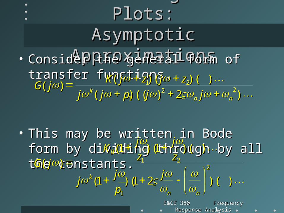
Constructing Bode Constructing Bode PlotsPlots
• CalculateCalculate the the complex number complex number GG((jj) ) for several frequencies for several frequencies and plot the points.and plot the points.
• Use Use MatLabMatLab to to automatically plot the automatically plot the Bode plots.Bode plots.
• Use Use asymptotic asymptotic approximationsapproximations..
E&CE 380 Frequency Response AnalysisE&CE 380 Frequency Response Analysis
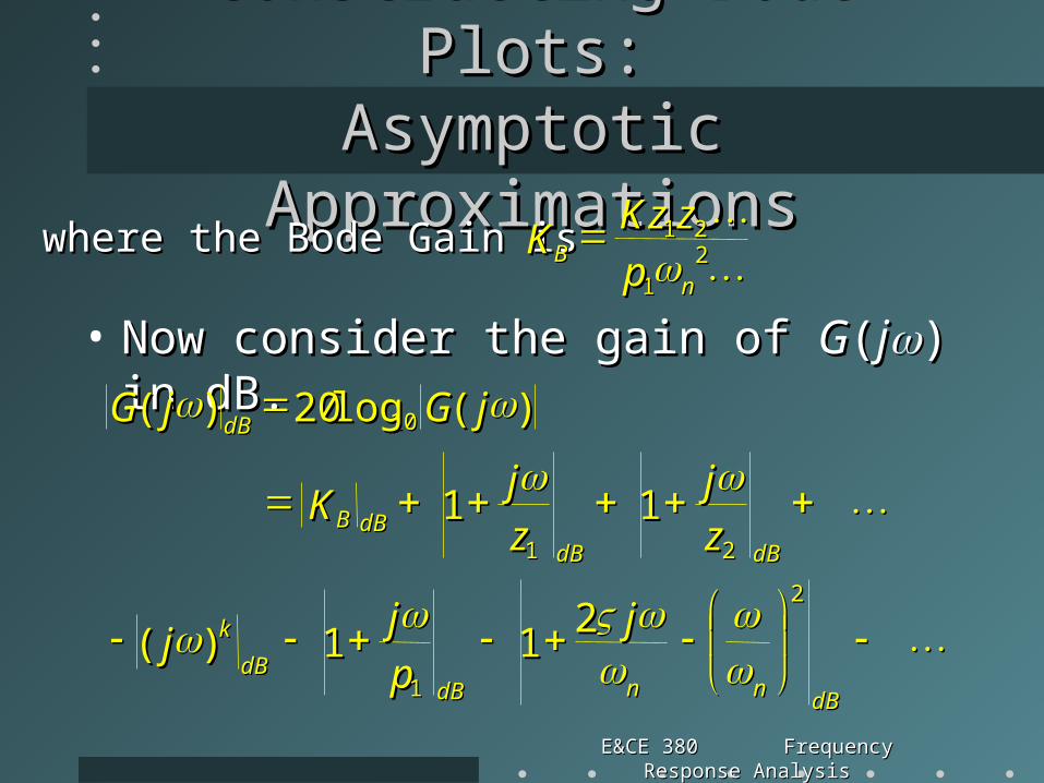
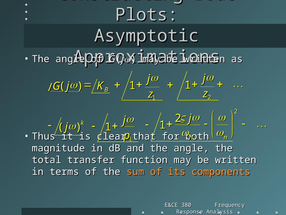
• The angle of The angle of GG((jj) may be written as) may be written as
• Thus it is clear that for both magnitude in dB Thus it is clear that for both magnitude in dB and the angle, the total transfer function may be and the angle, the total transfer function may be written in terms of the written in terms of the sum of its componentssum of its components
11
11))(( kk
ppjj
jj
22
2211
nnnn
jj
2211
1111 ))((// BB zzjj
zzjj
KKjjGG
E&CE 380 Frequency Response AnalysisE&CE 380 Frequency Response Analysis
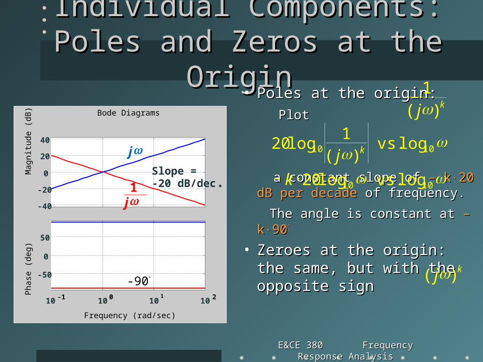
Individual Components:Individual Components:Poles and Zeros at the OriginPoles and Zeros at the Origin
• Poles at the origin:Poles at the origin:
PlotPlot
a constant slope of a constant slope of – k– k20 dB per20 dB per decadedecade of frequency. of frequency.
The angle is constant at The angle is constant at – k– k9090
• Zeroes at the origin:Zeroes at the origin:the same, but with the opposite the same, but with the opposite signsign
kj )(1
1010
1010
log vs.log20
log vs.)(
1log20
k
j k
kj )(
Frequency (rad/sec)
Ph
ase
(d
eg
)
M
ag
nitu
de
(d
B)
Bode Diagrams
-40
-20
0
20
40
10 -1 10 0 10 1
10 2
-50
0
50
j1
j
-90
Slope =-20 dB/dec.
E&CE 380 Frequency Response AnalysisE&CE 380 Frequency Response Analysis
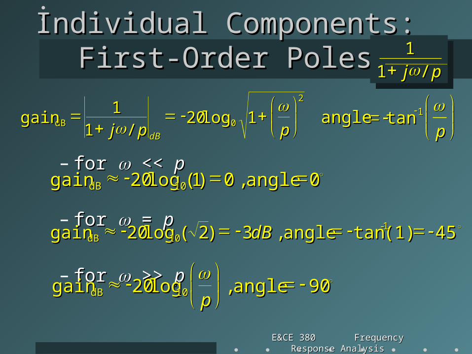
Individual Components:Individual Components:First-Order PolesFirst-Order Poles
E&CE 380 Frequency Response AnalysisE&CE 380 Frequency Response Analysis
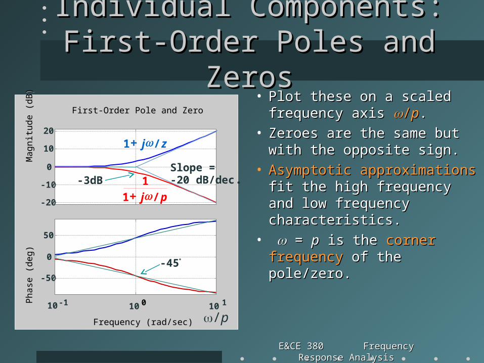
Individual Components:Individual Components:First-Order Poles and ZerosFirst-Order Poles and Zeros
• Plot these on a scaled Plot these on a scaled frequency axis frequency axis //pp..
• Zeroes are the same but with Zeroes are the same but with the opposite sign.the opposite sign.
• Asymptotic approximationsAsymptotic approximations fit the high frequency and fit the high frequency and low frequency characteristics.low frequency characteristics.
• = = pp is the is the corner frequencycorner frequency of the pole/zero.of the pole/zero.
Frequency (rad/sec)Frequency (rad/sec)
Pha
se (
deg)
M
agni
tude
(dB
)P
hase
(de
g)
Mag
nitu
de (
dB)
First-Order Pole and ZeroFirst-Order Pole and Zero
-20
-10
0
10
20
10 -1 10 0 10 1
-50
0
50
/p
pj /1
1
zj /1
Slope =-20 dB/dec.-3dB
-45
E&CE 380 Frequency Response AnalysisE&CE 380 Frequency Response Analysis
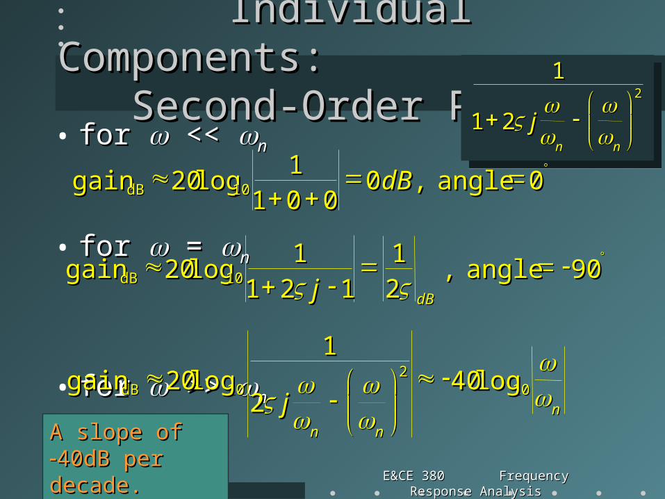
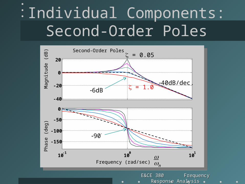
Individual Components:Individual Components: Second-Order Poles Second-Order Poles• for for << << nn
• for for = = nn
• for for >> >> nn
22
2211
11
nnnn
jj
000011
00angleangle,,00
11loglog2020gaingain 1010dBdB dBdB
9090angleangle,,2211
11221111
loglog2020gaingain 1010dBdB
dBdBjj
nn
nnnn
jj
1010
221010dBdB loglog4040
22
11
loglog2020gaingain
A slope of A slope of 40dB 40dB per decade.per decade.
E&CE 380 Frequency Response AnalysisE&CE 380 Frequency Response Analysis
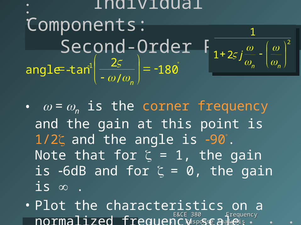
Individual Components: Second-Order Poles
• = n is the corner frequency and the gain at this point is 1/2and the angle is 90. Note that for = 1, the gain is 6dB and for = 0, the gain is .
• Plot the characteristics on a normalized frequency scale.
180/
2tan- angle 1-
n
2
21
1
nn
j
E&CE 380 Frequency Response AnalysisE&CE 380 Frequency Response Analysis
Individual Components:Second-Order Poles
Frequency (rad/sec)Frequency (rad/sec)
Pha
se (
deg)
M
agni
tude
(dB
)P
hase
(de
g)
Mag
nitu
de (
dB)
Second-Order PolesSecond-Order Poles
-40
-20
0
20
10-1
100
101
-150
-100
-50
0
nn
40dB/dec.6dB
= 0.05
= 1.0
90
E&CE 380 Frequency Response AnalysisE&CE 380 Frequency Response Analysis
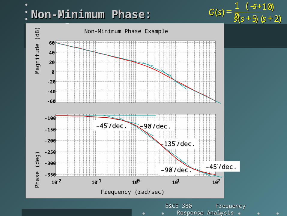
Individual Components:Non-Minimum Phase
• Non-minimum phase refers to a system with a final phase more negative than expected from the order of denominator and numerator.
• A zero in the RHS, (s + z) has the same magnitude characteristics as the zero in the LHS, but has the opposite angle. The final angle is 90 rather than +90 .
• The final phase of a system with a RHS zero will be 180 more negative than with a LHS zero
E&CE 380 Frequency Response AnalysisE&CE 380 Frequency Response Analysis
Individual Components:Non-Minimum Phase
• A second non-minimum phase component is a time delay or transportation lag which is represented by es, where is the delay time in seconds.
• The frequency characteristic is ej. The magnitude is 1.0 (0dB) for all frequencies and so it does not affect the magnitude plot.
• The phase angle is . When plotted against log10, this results in an exponential decrease in phase.
se
E&CE 380 Frequency Response AnalysisE&CE 380 Frequency Response Analysis
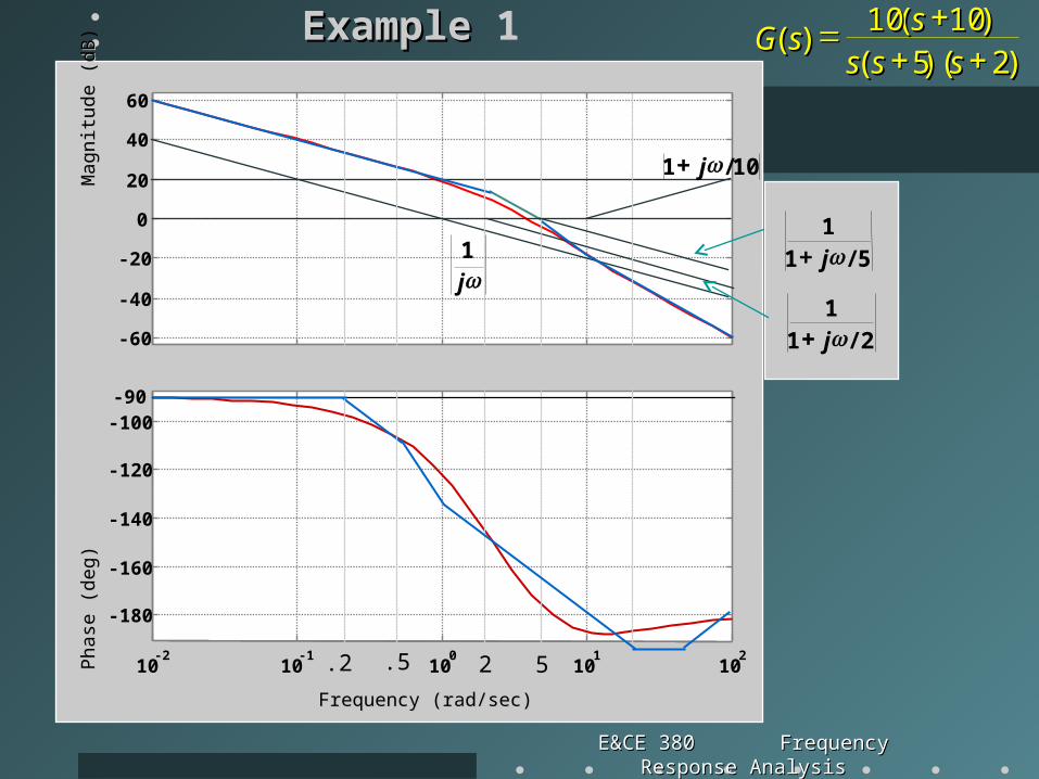
Bode Plot Construction:Bode Plot Construction: Example 1 Example 1
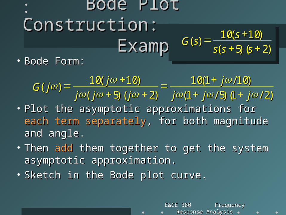
• Bode Form:Bode Form:
• Plot the asymptotic approximations for Plot the asymptotic approximations for each term each term separatelyseparately, for both magnitude and angle., for both magnitude and angle.
• Then Then addadd them together to get the system them together to get the system asymptotic approximation.asymptotic approximation.
• Sketch in the Bode plot curve.Sketch in the Bode plot curve.
))22)()(55(())1010((1010
))((
ssssss
ssssGG
))22//11)()(55//11(())1010//11((1010
))22)()(55(())1010((1010
))((
jjjjjjjj
jjjjjjjj
jjGG
E&CE 380 Frequency Response AnalysisE&CE 380 Frequency Response Analysis
))22)()(55(())1010((1010
))((
ssssss
ssssGGExampleExample 1
5/1
1j
2/1
1j
Frequency (rad/sec)Frequency (rad/sec)
Pha
se (
deg)
Mag
nitu
de (
dBP
hase
(de
g)
M
agni
tude
(dB
)
-60
-40
-20
0
20
40
60
10-2
10-1
100
101
102
-180
-160
-140
-120
-100
j1
2 5.2 .5
-90
10/1 j
E&CE 380 Frequency Response AnalysisE&CE 380 Frequency Response Analysis
))22)()(55(())1010(–(–11
00))((
ssssss
ssssGGNon-Minimum Phase: Example 1ANon-Minimum Phase: Example 1A
Frequency (rad/sec)Frequency (rad/sec)
Pha
se (
deg)
M
agni
tude
(dB
)P
hase
(de
g)
Mag
nitu
de (
dB)
Non-Minimum Phase ExampleNon-Minimum Phase Example
-60
-40
-20
0
20
40
60
10-2 10-1 100 101 102-350
-300
-250
-200
-150
-100
––4545/dec./dec. ––9090/dec./dec.
––135135/dec./dec.
––4545/dec./dec.––9090/dec./dec.
E&CE 380 Frequency Response AnalysisE&CE 380 Frequency Response Analysis
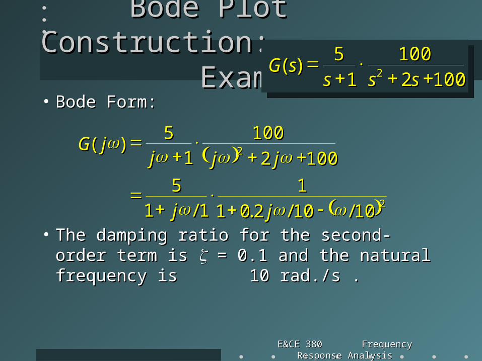
Bode Plot Construction:Bode Plot Construction: Example 2 Example 2• Bode Form:Bode Form:
• The damping ratio for the second-order term is The damping ratio for the second-order term is = 0.1 and the natural frequency is 10 = 0.1 and the natural frequency is 10 rad./s .rad./s .
10010022100100
1155
))(( 22
ssssssssGG
22
22
1010//1010//22..001111
11//1155
10010022100100
1155
))((
jjjj
jjjjjjjjGG
E&CE 380 Frequency Response AnalysisE&CE 380 Frequency Response Analysis
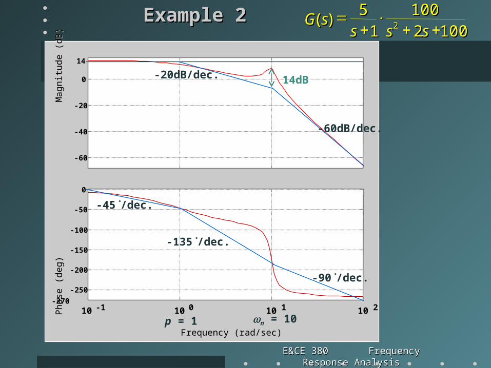
Example 2Example 2
Frequency (rad/sec)Frequency (rad/sec)
Pha
se (
deg)
M
agni
tude
(dB
)P
hase
(de
g)
Mag
nitu
de (
dB)
-60
-40
-20
0
10 -1 10 0 10 1 10 2
-250
-200
-150
-100
-50
0
14
-60dB/dec.
-20dB/dec.
-270
p = 1 n = 10
-45/dec.
-135/dec.
-90/dec.
14dB
10010022100100
1155
))(( 22
ssssssssGG
E&CE 380 Frequency Response AnalysisE&CE 380 Frequency Response Analysis
Transfer Function Identification• Frequency response characteristics can be be obtained
experimentally by applying sinusoidal inputs of various frequencies, and measuring the gain and phase relationships between input and output.
• By fitting asymptotic approximations to the frequency response characteristics obtain from experimental measurements, an approximate transfer function model of the system can be obtained.
E&CE 380 Frequency Response AnalysisE&CE 380 Frequency Response Analysis
Transfer Function Identification:Major Steps
1. Determine the initial slope order of poles at the origin.
2. Determine the final slope difference in order between the denominator and numerator (nm).
3. Determine the initial and final angle confirm the results from above or detect the presence of a non-minimum phase system (delays or zeroes in the RHS).
4. Determine the low frequency gain (Bode gain).
E&CE 380 Frequency Response AnalysisE&CE 380 Frequency Response Analysis
Transfer Function Identification:Major Steps
5. Detect the number and approximate location of corner frequencies and fit asymptotes.– possibly subtract well defined components.– examine expected -3dB points.– try to separate second-order terms and use the
standard responses to estimate damping.
6. Sketch the phase plot for the identified transfer function as a check of accuracy.
E&CE 380 Frequency Response AnalysisE&CE 380 Frequency Response Analysis
Transfer Function Identification:Major Steps
7. Use the phase plot to check for non-minimum phase terms and to calculate the time delay value if one is present.
8. Calculate the frequency response for the identified model and check against the experimental data (MatLab or a few points by hand calculation).
9. Iterate and refine the pole/zero locations and damping of second-order terms.
E&CE 380 Frequency Response AnalysisE&CE 380 Frequency Response Analysis
Frequency (rad/sec)Frequency (rad/sec)
Ph
ase
(deg
)
Mag
nit
ud
e (d
BP
has
e (d
eg)
M
agn
itu
de
(dB
)
)
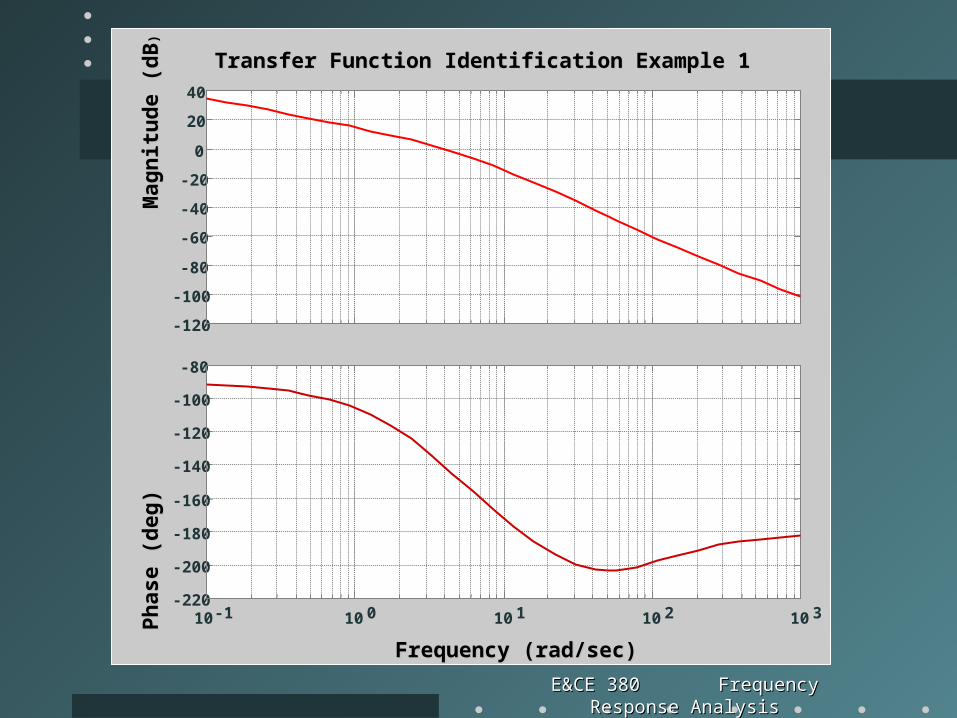
Transfer Function Identification Example 1Transfer Function Identification Example 1
-120
-100
-80
-60
-40
-20
0
20
40
10 -1 10 0 10 1 10 2 10 3-220
-200
-180
-160
-140
-120
-100
-80
E&CE 380 Frequency Response AnalysisE&CE 380 Frequency Response Analysis
Transfer Function Model Transfer Function Model Identification: Example 1Identification: Example 1
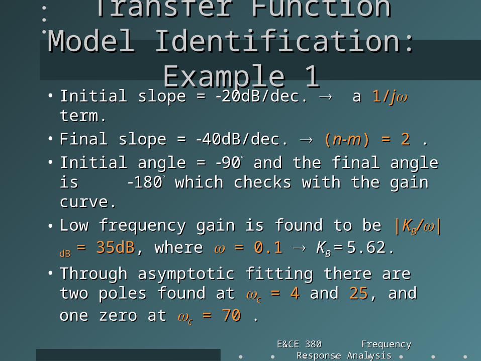
• Initial slope = Initial slope = 20dB/dec. 20dB/dec. a a 1/1/jj term. term.
• Final slope = Final slope = 40dB/dec. 40dB/dec. ((n-mn-m) = 2) = 2 . .
• Initial angle = Initial angle = 9090 and the final angle is and the final angle is 180180 which checks with the gain curve. which checks with the gain curve.
• Low frequency gain is found to be Low frequency gain is found to be ||KKBB//||dB dB = =
35dB35dB, where , where = 0.1 = 0.1 KKB B = = 5.625.62 . .
• Through asymptotic fitting there are two Through asymptotic fitting there are two poles found at poles found at cc = 4 = 4 and and 2525, and one zero at , and one zero at
cc = 70 = 70 . .
E&CE 380 Frequency Response AnalysisE&CE 380 Frequency Response Analysis
Frequency (rad/sec)Frequency (rad/sec)
Ph
ase
(deg
)
Mag
nit
ud
e (d
BP
has
e (d
eg)
M
agn
itu
de
(dB
)
)
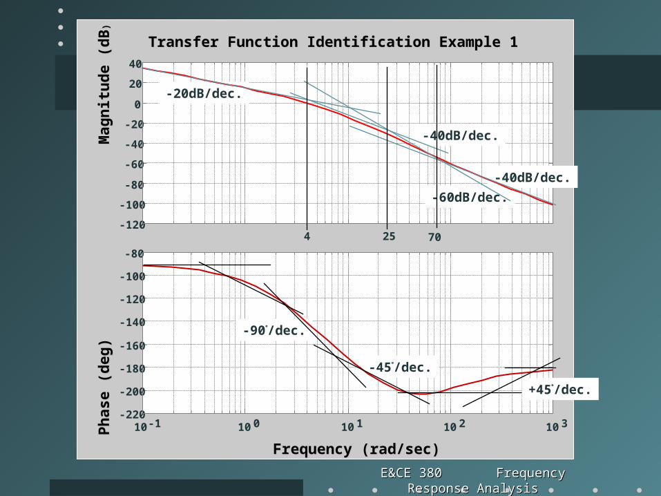
Transfer Function Identification Example 1Transfer Function Identification Example 1
-120
-100
-80
-60
-40
-20
0
20
40
10 -1 10 0 10 1 10 2 10 3-220
-200
-180
-160
-140
-120
-100
-80
-20dB/dec.
-40dB/dec.
-60dB/dec.
-40dB/dec.
4 25 70
-45/dec.
-90/dec.
+45/dec.
E&CE 380 Frequency Response AnalysisE&CE 380 Frequency Response Analysis
Transfer Function Model Transfer Function Model Identification: Example 1Identification: Example 1
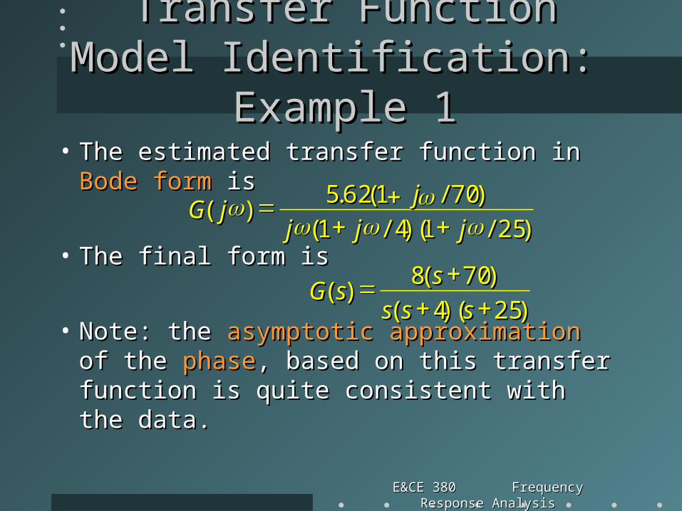
• The estimated transfer function in The estimated transfer function in Bode formBode form isis
• The final form isThe final form is
• Note: the Note: the asymptotic approximationasymptotic approximation of the of the phasephase, based on this transfer function is quite , based on this transfer function is quite consistent with the data.consistent with the data.
))2525)()(44(())7070((88
))((
ssssssss
ssGG
))2525//11)()(44//11((
))7070//11((6262..55))((
jjjjjjjj
jjGG
E&CE 380 Frequency Response AnalysisE&CE 380 Frequency Response Analysis
Frequency (rad/sec)Frequency (rad/sec)
Ph
ase
(deg
)
Mag
nit
ud
e (d
B)
Ph
ase
(deg
)
Mag
nit
ud
e (d
B)
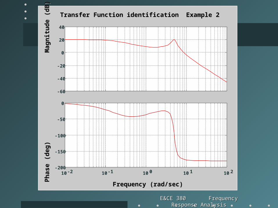
Transfer Function identification Example 2Transfer Function identification Example 2
-60
-40
-20
0
20
40
10 -2 10 -1 10 0 10 1 10 2-200
-150
-100
-50
0
E&CE 380 Frequency Response AnalysisE&CE 380 Frequency Response Analysis
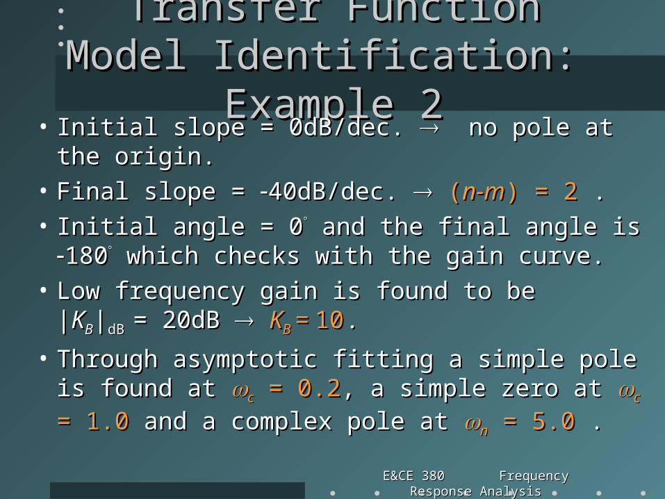
Transfer Function Model Transfer Function Model Identification: Example 2Identification: Example 2
• Initial slope = 0dB/dec. Initial slope = 0dB/dec. no pole at the origin. no pole at the origin.• Final slope = Final slope = 40dB/dec. 40dB/dec. ((n-mn-m) = 2) = 2 . .• Initial angle = 0Initial angle = 0 and the final angle is and the final angle is 180180 which which
checks with the gain curve.checks with the gain curve.• Low frequency gain is found to beLow frequency gain is found to be
||KKBB||dB dB = 20dB = 20dB KKB B = = 1010 . .
• Through asymptotic fitting a simple pole is found Through asymptotic fitting a simple pole is found at at cc = 0.2 = 0.2,, a simple zero ata simple zero at cc = 1.0 = 1.0 and a and a
complex pole at complex pole at nn = 5.0 = 5.0 . .
E&CE 380 Frequency Response AnalysisE&CE 380 Frequency Response Analysis
Frequency (rad/sec)Frequency (rad/sec)
Ph
ase
(deg
)
Mag
nit
ud
e (d
B)
Ph
ase
(deg
)
Mag
nit
ud
e (d
B)
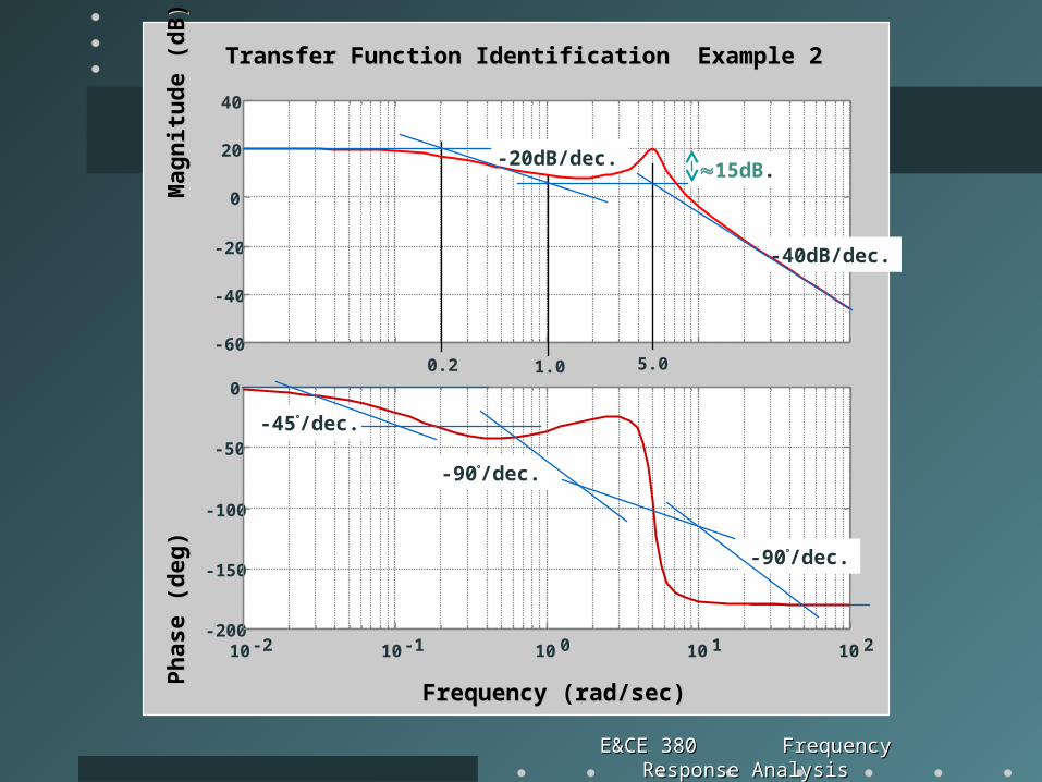
Transfer Function Identification Example 2Transfer Function Identification Example 2
-60
-40
-20
0
20
40
10 -2 10 -1 10 0 10 1 10 2-200
-150
-100
-50
0 0.2 1.0 5.0
-40dB/dec.
-20dB/dec.
-45/dec.
-90/dec.
-90/dec.
15dB.
E&CE 380 Frequency Response AnalysisE&CE 380 Frequency Response Analysis
Transfer Function Model Transfer Function Model Identification: Example 2Identification: Example 2
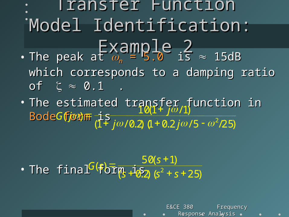
• The peak at The peak at nn = 5.0 = 5.0 is is 15dB which 15dB which
corresponds to a damping ratio of corresponds to a damping ratio of 0.1 . 0.1 .
• The estimated transfer function in The estimated transfer function in Bode formBode form is is
• The final form isThe final form is
)25)(2.0()1(50
)( 2
ssss
sG
)25/5/2.01)(2.0/1()1/1(10
)( 2
jjj
jG
E&CE 380 Frequency Response AnalysisE&CE 380 Frequency Response Analysis
Frequency (rad/sec)Frequency (rad/sec)
Pha
se (
deg)
Mag
nitu
de
(dB
)P
hase
(de
g)
M
agn
itud
e (d
B)
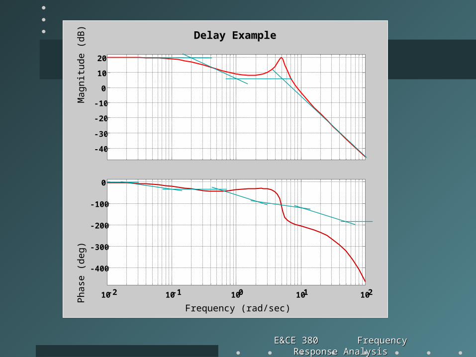
Delay ExampleDelay Example
-40
-30
-20
-10
0
10
20
10-2 10-1 100 101 102
-400
-300
-200
-100
0
E&CE 380 Frequency Response AnalysisE&CE 380 Frequency Response Analysis
Transfer Function Model Transfer Function Model Identification: Example 2AIdentification: Example 2A
• The magnitude plot is the same as the previous The magnitude plot is the same as the previous example.example.
• The angle plot continues to go more negative The angle plot continues to go more negative and and does notdoes not asymptotically approach asymptotically approach 180180 as as expected.expected.
• This is a non-minimum phase system with a This is a non-minimum phase system with a time delay, time delay, ee–s–s..
• How do we determine the time delay,How do we determine the time delay, ? ?
E&CE 380 Frequency Response AnalysisE&CE 380 Frequency Response Analysis
Transfer Function Model Transfer Function Model Identification: Example 2AIdentification: Example 2A
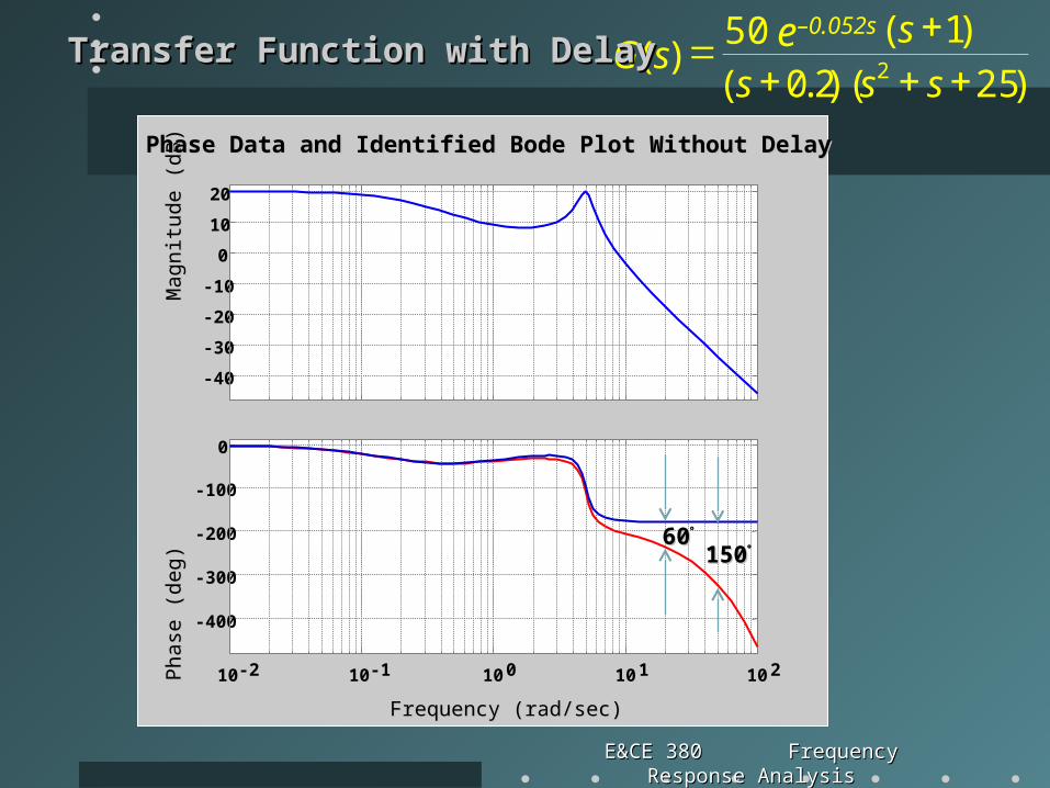
• Plot the phase of the transfer function identified from the magnitude plot and find the phase difference between this plot and the phase data.
• This difference represents the ee–j–jterm.term.
• At At = 20 = 20 rad/sec, – rad/sec, – – –/3 /3 0.052 s 0.052 s (– 60(– 60) )
• At At = 50 = 50 rad/sec, – rad/sec, – – 5 – 5/6 /6 0.052 s 0.052 s (– 150(– 150) )
E&CE 380 Frequency Response AnalysisE&CE 380 Frequency Response Analysis
Frequency (rad/sec)Frequency (rad/sec)
Pha
se (
deg)
Mag
nitu
de (
dB)
Pha
se (
deg)
Mag
nitu
de (
dB)
Phase Data and Identified Bode Plot Without DelayPhase Data and Identified Bode Plot Without Delay
-40
-30
-20
-10
0
10
20
10 -2 10 -1 10 0 10 1 10 2
-400
-300
-200
-100
0
6060
150150
)25)(2.0(
)1(50)( 2
sss
ssG
e–0.052sTransfer Function with DelayTransfer Function with Delay
E&CE 380 Frequency Response AnalysisE&CE 380 Frequency Response Analysis
Bode Plots and Stability AnalysisBode Plots and Stability Analysis• In the In the NyquistNyquist analysis, it became clear that analysis, it became clear that
Section II of the plot was the most critical in Section II of the plot was the most critical in determining the stability of the closed-loop system.determining the stability of the closed-loop system.
• The The Bode plotBode plot of the loop transfer function, of the loop transfer function, GHGH((jj)) provides the same magnitude and angle provides the same magnitude and angle information as Section II of the Nyquist plot.information as Section II of the Nyquist plot.
• Therefore, the Bode plot of Therefore, the Bode plot of GHGH((jj) can be used to ) can be used to evaluate the evaluate the stability of the closed-loopstability of the closed-loop system. system.
E&CE 380 Frequency Response AnalysisE&CE 380 Frequency Response Analysis
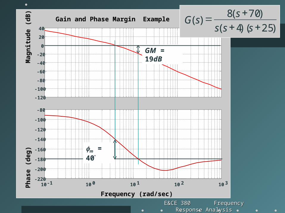
Bode Plots and Stability AnalysisBode Plots and Stability Analysis• Consider the definitions of the gain and phase margins Consider the definitions of the gain and phase margins
in relation to the Bode plot of in relation to the Bode plot of GHGH((jj) .) .– Gain MarginGain Margin: the : the additional gainadditional gain required to make required to make
| | GHGH((jj) | = 1) | = 1 when when //GHGH((jj)) = = 180180 . On the Bode plot this . On the Bode plot this is the distance, in is the distance, in dBdB, from the magnitude curve up to 0, from the magnitude curve up to 0dBdB when the angle curve crosses when the angle curve crosses 180180 ..
– Phase MarginPhase Margin: the : the additional phase lagadditional phase lag required to make required to make //GHGH((jj)) = = 180180 whenwhen | | GHGH((jj) | = 1) | = 1 . On the Bode plot this . On the Bode plot this is the distance in degrees from the phase curve to is the distance in degrees from the phase curve to 180180 when the gain curve crosses 0when the gain curve crosses 0dBdB..
E&CE 380 Frequency Response AnalysisE&CE 380 Frequency Response Analysis
Frequency (rad/sec)Frequency (rad/sec)
Ph
ase
(deg
)
Mag
nit
ud
e (d
B)
Ph
ase
(deg
)
Mag
nit
ud
e (d
B)
Gain and Phase Margin ExampleGain and Phase Margin Example
-120
-100
-80
-60
-40
-20
0
20
40
10 -1 10 0 10 1 10 2 10 3-220
-200
-180
-160
-140
-120
-100
-80
GM = 19dB
m = 40
)25)(4(
)70(8)(
sss
ssG
E&CE 380 Frequency Response AnalysisE&CE 380 Frequency Response Analysis
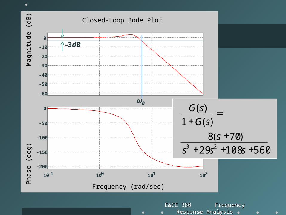
Closed-loop Frequency ResponseClosed-loop Frequency Response• Assuming the closed-loop system is stable, the Assuming the closed-loop system is stable, the
frequency response of the closed-loop system will frequency response of the closed-loop system will directly give the directly give the bandwidthbandwidth of the system, i.e. of the system, i.e. 33dBdB down from the steady-state gaindown from the steady-state gain..
• This will be related to the zero crossing frequency of This will be related to the zero crossing frequency of the loop transfer function plot.the loop transfer function plot.
• Information about the Information about the overshootovershoot of the step response of the step response can also be obtained from the can also be obtained from the peak of the magnitudepeak of the magnitude curve in the closed-loop Bode plot.curve in the closed-loop Bode plot.
E&CE 380 Frequency Response AnalysisE&CE 380 Frequency Response Analysis


![G ] e s t o s i s](https://static.documents.pub/doc/80x56/62322b787a682452315b4765/g-e-s-t-o-s-i-s.jpg)

![g n v R | S | U g R ¾ d e Y R W S [ v R i e W e S n Y R …...(Franciscans) (94) S j j g } R-3 U g i s Y U ] x T Y g T Z U c)))) g T) g .))](https://static.documents.pub/doc/80x56/5e2b0ff1c91523374e6767e0/g-n-v-r-s-u-g-r-d-e-y-r-w-s-v-r-i-e-w-e-s-n-y-r-franciscans-94.jpg)


