Frequency Selective Model Order Reduction via Spectral Zero Projection

Mehboob Alam Arthur Nieuwoudt Yehia Massoud

Department of Electrical and Computer Engineering

Rice University

Houston, TX 77005

Tel: 713-348-6706

Fax: 713-348-6196

e-mail: {alam,abnieu,massoud}@rice.edu

Abstract— As process technology continues to scale into thenanoscale regime, interconnect plays an ever increasing role in de-termining VLSI system performance. As the complexity of thesesystems increases, reduced order modeling becomes critical. Inthis paper, we develop a new method for the model order reduc-tion of interconnect using frequency restrictive selection of inter-polation points based on the spectral-zeros of the RLC intercon-nect model’s transfer function. The methodology uses the imagi-nary part of spectral zeros for frequency selective projection andprovides stable as well as passive reduced order models for in-terconnect in VLSI systems. For large order interconnect mod-els with realistic RLC parameters, the results indicate that ourmethod provides more accurate approximations than techniquesbased on balanced truncation and moment matching with excel-lent agreement with the original system’s transfer function.

I. INTRODUCTION

Aggressive feature scaling and increasing operating frequen-

cies are greatly impacting the performance of high speed inte-

grated circuits [1], Motivated by the expanding complexity of

nanoscale integrated circuits, the model order reduction (MOR)

of RLC interconnect models has been the focal point of sub-

stantial research efforts over the last decade [2, 3, 4]. The

methods used for the MOR of interconnects fall into two main

categories: Singular Value Decomposition (SVD) methods and

Krylov subspace projection methods. In SVD methods for lin-

ear systems, Hankel-norm approximation, balanced truncation,

and singular perturbation methods are well known. The most

popular technique is balanced approximation, in which the pri-

mary aim is to generate a balanced representation of the system

with same degree of reachability and observability. Balanced

approximation based algorithms such as PMTBR [5, 6], PR-

TBR [7] and FABT [8, 9] have been proposed for intercon-

nect model order reduction. However, SVD methods have high

computational complexity with dense computations of ordern3

and storage of order n2. As such, these methods are not suited

for reducing systems with high complexity.

For large scale systems, moment-matching projection meth-

ods [10] provide a tractable alternative to SVD methods. In

general, projection methods consist of iterations involving

the controllability and reachability subspaces (also known as

Krylov subspaces) spanned by a sequence of vectors. These

methods provide an iterative approximation of the eigenvalues

in order to match the system’s moments. A number of Krylov-

basedmodel order reduction implementations [11, 3] have been

proposed. These methods are attractive due to their iterative na-

ture and are computationally less expensive than balanced ap-

proximation. However, unlike balanced approximation meth-

ods, there is typically no guarantee of stability or an upper error

bound.

High performance interconnects have a frequency dependent

resistance and reactance that give rise to complex frequency

responses [9, 12]. The complex frequency response usually

gives rise to high frequency variations. To match these varia-

tions, a high order system is typically required to approximate

the original system response. This is computationally expen-

sive and may not be suitable for large scale VLSI systems.

In order to efficiently approximate large variations in the fre-

quency response, a frequency selective model order reduction

technique is well-suited to provide low order approximations

and to match the original system response over a given range

of frequencies.

In this paper, we develop a passivity preserving model order

reduction method with frequency selective interpolation points

derived from imaginary part of the spectral zeros of the sys-

tem. The reduced model preserves the properties of the origi-

nal system as well as the stability and passivity. The preserva-

tion of passivity is guaranteed by selecting interpolation points

as a subset of the stable system’s spectral zeros. The MOR

technique is implemented using Krylov projection methods to

ensure low complexity. The results indicate that our method

provides more accurate approximations than techniques based

on balanced truncation and moment matching.

II. MODEL ORDER REDUCTION PROBLEM FORMULATION

An RLC representation for a linear dynamic system can be

written using following state space representation:

Ex = Ax + Bu (1)

y = Cx + Du

where E ∈ �nxn, A ∈ �nxn, B ∈ �nxm, C ∈ �pxn andD ∈�pxm are the matrices defining the linear maps between inputs,

1-4244-0630-7/07/$20.00 ©2007 IEEE.

4A-5

379

outputs, and internal state variables generated using common

techniques such as modified nodal analysis. Without loss of

generality, we will assume E to be identity for the purpose of

theoretical analysis. We represent the state space system as a

linear dynamic system using the following representation

Σ =

[A|B

C|D

]∈ �(n+p)x(n+m). (2)

We then approximate the system using the following reduced

model order formulation

Σ =

[A|B

C|D

]∈ �(k+p)x(k+m) (3)

where k << n. When W ∗ and V are orthogonal (W ∗V =Ik)

and span the reduced order subspace, the reduced system is of

the form

A = W ∗AV, (4)

B = W ∗B,

C = CV,

D = D

where order of A << A. The most popular technique for com-

puting the orthogonal projectors used to generate the reduced

system is the Block Arnoldi method, which has been the basis

for several previous techniques [3, 13, 14]. The Block Arnoldi

method iteratively produces basis vectors of the following form

AVk = VkHk + rke∗k (5)

where Vk are the orthogonal basis vectors generated at iteration

k of the algorithm. Arnoldi implicitly forms the basis vectors

that span the Krylov subspace defined as

K(A, B) = [B, AB, A2B · · ·Ak−1B]. (6)

Several issues complicate the implementation of Krylov-based

projection methods. Numerical issues may cause the basis vec-

tors (Hk) to lose orthogonality, thereby corrupting the projec-

tors and mitigating the effectiveness of the reduced system ap-

proximation. The reduced system may also not be stable or

passive unless certain methods are employed [3, 14]. Since the

Arnoldi iteration first approximates the eigenvalues associated

with the high-frequency poles of the system, it may produce

reduced order models that do not match the original system’s

response in the frequencies of interest. By applying shifted-

Arnoldi to provide a multi-point interpolation of reduced sys-

tems at a different frequency points, the function can be ap-

proximated across a wide-range of frequencies [15]. However,

choosing these interpolation points to minimize the computa-

tional complexity may be problematic.

In the following sections, we derive and implement a new

method for choosing interpolation points based on the spectral

zeros of the system’s transfer function to match over the desired

frequency range. The method preserves the passivity of the

reduced order system by construction.

III. MODEL ORDER REDUCTION WITH

PRESERVATION OF PASSIVITY

Our proposed method of model order reduction with preser-

vation of passivity is based on the frequency selective posi-

tive real interpolation of linear time invariant systems. The

approach is inspired by frequency selection and projection of

systems with the desired dominant frequency band of interest.

The choice of interpolation points will guarantee the preser-

vation of passivity and can produce a lower order model when

compared with techniques such as balanced truncation and mo-

ment matching.

It is known that the passivity of a linear time invariant sys-

tem is preserved if its transfer function, G(s), is positive real.The positive realness of the Σ system is achieved if the transferfunction satisfies the following conditions [16, 17]:

1. G(s) is analytical for Re(s) > 0;2. G(s) = G(s) for all s ∈ C; and

3. G(s) + G(s)∗ ≥ for Re(s) > 0.

The second condition is satisfied for real systems and the

third condition implies the existence of a rational function with

a stable inverse. Therefore, there exists a set of projectors, V

andW ∗ with V W ∗ = 0 with V W ∗ �= 0 obtained by interpo-lating the transfer function so that the projected system is both

stable and passive. As a result, we seek interpolation points

that are positive real. In the linear system Σ defined in (2), (A,B) are reachable and (C, A) are observable. The matrix A is

also assumed to be stable with eigenvalues residing in the open

left-hand plane. The system passivity is then equivalent to the

positive realness of the associated transfer function

G(s) = D + C(sI − A)−1B. (7)

The spectral zeros of a system are defined as the zeros of thequantityG(s) + G(−s). Furthermore, it is true that

G(s) + G(−s) =r(s)r(−s)

d(s)d(−s), (8)

where d(s) and n(s) are the denominator and numerator of thetransfer function, respectively, and

r(s)r(−s) = n(s)d(−s) + d(s)n(−s). (9)

The roots of the polynomial r(s) are in the closed left-handplane and the coefficients are real. This means that the spec-

tral zeros cannot be purely imaginary. Additionally, the stablespectral zeros are defined as the roots of r(s). In terms of thesystem matrices, the stable spectral zeros are all λ that satisfy

Υ − λΦ = 0 (10)

where

Υ =

⎡⎣ A 0 B

0 −A∗ −C∗

C B∗ D + D∗

⎤⎦

Φ =

⎡⎣ E 0 0

0 E 00 0 0

⎤⎦ . (11)

4A-5

380

1010

1011

1012

−8

−6

−4

−2

0

2

4

6

8x 10

12

Real

Imag

inar

y

Spectral ZerosSelected Spectral Zeros

Selected Spectral Zeros

Fig. 1. Spectral zeros of an RLC circuit model with frequency selectivespectral zeros maked by ∗.

Moreover, if D + D∗ is invertible, these numbers are the gen-

eralized eigenvalues of the following Hamiltonianmatrix:[A 00 −A∗

]−

[B

−C∗

](D + D∗)−1(CB∗). (12)

The critical result is that if the interpolation points are cho-

sen to be the spectral zeros of the original system Σ, the re-duced system is both stable and passive. Equation (11) shows

that the method can also be applied to systems in descrip-

tor form. In our implementation, we have used Implicitly

Restarted Arnoldi to solve the generalized eigenvalue problem

to handle higher order systems [18]. This makes the computa-

tional cost comparable to Krylovmethods (O(kN 2)) and muchless than balanced truncation methods (O(N 3)). The eigenval-ues are the spectral zeros and lie on the left-half plane since

G∗(−λi) + G∗(λi) = 0.The generalized eigenvalues λ defined in (10) are the spec-

tral zeros of a given system. In order to obtain an accurate

approximation of the original system for the frequencies of in-

terest, we need to choose appropriate finite spectral zeros to

use as interpolation points. Figure 1 shows the spectral ze-

ros of an RLC circuit model and the selected spectral zeros.

We select the spectral zeros with imaginary part near the fre-

quency of interest to match the response close to the selected

frequency. In addition, for each spectral zero selected, we se-

lected its complex conjugate. Therefore, each spectral zero se-

lected as an interpolation point increases the reduced system

order by 2. Once we have chosen the spectral zeros, we use the

eigenvectors (Q) corresponding to the selected spectral zerosto construct the projectors V and W . In the implementation

of the proposed scheme, the state dimension of the model will

be reduced to k with k � n. Assuming V W ∗ �= 0, the pro-jected system Σ can interpolate the system transfer function atsi, i = 1, ..., 2k. The projectors V and W are used to reduce

the system in the following manner:

B = W ∗B, C = CV, E = W ∗EV, D = D. (13)

AlgorithmCn Gn Bn Ln

GnBnLnCnDn

Fig. 2. Pseudocode of frequency selective passivity preserving MORalgorithm.

TABLE I

DESIGN PROBLEM CHARACTERISTICS

RLC Inductor

Order 79 1008

Permuted Order 77 981

Reduced Order 28 64

Minimum Frequency (rads/sec) 109 109

Maximum Frequency (rads/sec) 1014 1014

Condition number (E−1G) 4.0189x1010 2.5309x1013

Condition numberA 801.1024 1.2909x105

Condition numberE ∞ ∞

The algorithm for the selection of spectral zeros is shown in

Figure 2. The frequency selection is performed using the ab-

solute value of the imaginary part of the spectral zeros. The

selected spectral zeros are then used to identify corresponding

eigenvectors, which are used to construct the projectors V and

W of the system. These projectors are orthogonal and dynam-

ically generate reduced order model.

IV. RESULTS

The first structure simulated is a simple RLC circuit repre-

senting an interconnect wire. The circuit used to model the

structure is presented in Figure 3(a). The model takes into

account the resistance, inductance, self-capacitance, coupling-

capacitance, and mutual-inductance between the segments in

the interconnect wire. Note that in Figure 3(a), not all of the

coupling-capacitances and mutual inductances are shown. In

creating state space models for the simulated circuit, we used

the field solvers FastCap and FastHenry for capacitance and

inductance extraction [19, 20] and finally combine the results

using modified nodal analysis [3]. The complexity of the ini-

tial system is n = 77. The original system is compared against

4A-5

381

Err

or

(a)

(b)

(c)

Fig. 3. System frequency response (a, b) and error (c) for an RLC networkwith original and reduced models of order n = 79 and n = 28, respectively.

model reductions performed by our proposed technique, bal-

anced truncation, and the Arnoldi based PRIMA method [3].

The order and condition of the system matrices is given by Ta-

ble I. It can be noted that matrix A is ill-conditioned, which

often leads to poor performance of balance truncation method.

The original system matrix E is singular and needs to be per-

muted to remove the singularities. The permuted system re-

duces the order of the system from 79 to 77. In carrying out

PRIMA computation also similar ill-conditioning leads the up-

per Heisenberg matrix H to loose orthogonality at each itera-

tive step. To compensate for ill-conditioning of system DGKS

correction is applied at each iteration to avoid ill-conditioning

and maintaining orthogonality of basis vectors. Figure 3(a)

compares the frequency response of our method, PRIMA, and

balanced truncation with the original system. It shows that

an order 28 system generated by balanced truncation does not

(b)

(b)

(a)

(a)Top View

Side View

Spiral

(a)Top View

Side View Spiral

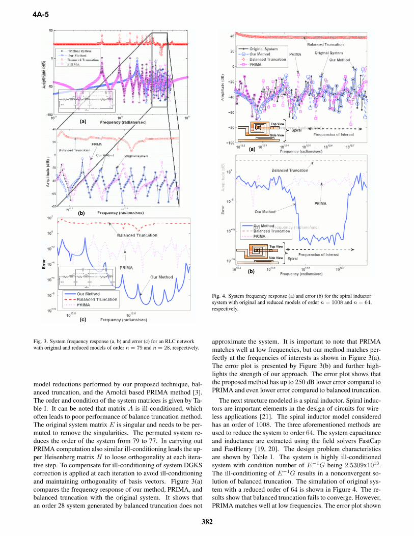
Fig. 4. System frequency response (a) and error (b) for the spiral inductorsystem with original and reduced models of order n = 1008 and n = 64,

respectively.

approximate the system. It is important to note that PRIMA

matches well at low frequencies, but our method matches per-

fectly at the frequencies of interests as shown in Figure 3(a).

The error plot is presented by Figure 3(b) and further high-

lights the strength of our approach. The error plot shows that

the proposed method has up to 250 dB lower error compared to

PRIMA and even lower error compared to balanced truncation.

The next structure modeled is a spiral inductor. Spiral induc-

tors are important elements in the design of circuits for wire-

less applications [21]. The spiral inductor model considered

has an order of 1008. The three aforementioned methods areused to reduce the system to order 64. The system capacitanceand inductance are extracted using the field solvers FastCap

and FastHenry [19, 20]. The design problem characteristics

are shown by Table I. The system is highly ill-conditioned

system with condition number of E−1G being 2.5309x1013.

The ill-conditioning of E−1G results in a nonconvergent so-

lution of balanced truncation. The simulation of original sys-

tem with a reduced order of 64 is shown in Figure 4. The re-sults show that balanced truncation fails to converge. However,

PRIMA matches well at low frequencies. The error plot shown

4A-5

382

in Figure 4(b) further highlights the strength of our method

and shows low error at the frequencies of interest compared to

PRIMA and balanced truncation. The example demonstrates

that for large scale systems, the proposed method accurately

approximates the original system.

V. CONCLUSION

In order to efficiently capture complex interconnect effects

in high performance VLSI systems, model order reduction can

provide tractable solutions to complex interconnect analysis

problems. In this paper, we present new method of model order

reduction for interconnects that uses the systematic selection of

the interpolation points to provide the advantage of generating

passive models. Our method is efficient as well as accurate and

generates stable reduced systems. The simulation results using

the new technique match closely with the results from the full

system. Additionally, the reduced order model preserves the

properties of the original system and due to its computational

performance, it can be effectively applied to reduce large scale

VLSI systems.

REFERENCES

[1] M. Mondal and Y. Massoud, “Reducing Pessimism in

RLCDelay Estimation Using an Accurate Analytical Fre-

quency Dependent Model for Inductance,” in Proceed-ings of ICCAD, November 2005, pp. 690–695.

[2] J. M. Wang, C.-C. Chu, Q. Yu, and E. S. Kuh, “On

Projection-Based Algorithms for Model-Order Reduction

of Interconnects,” IEEE Trans. Circuits Syst.- I, vol. 49,no. 11, pp. 1563–1585, November 2002.

[3] A. Odabasioglu, M. Celik, and L. T. Pileggi, “PRIMA:

Passive Reduced-Order Interconnect Macromodeling Al-

gorithm,” IEEE Trans. CAD, vol. 17, no. 8, pp. 645–654,August 1998.

[4] M. Kamon, F. Wang, and J. White, “Generating Nearly

Optimally Compact Models from Krylov-Subspace

Based Reduced-Order Models,” IEEE Trans. CircuitsSyst.- II, vol. 47, no. 4, pp. 239-248, April 2000.

[5] J. Phillips and L. M. Silveira, “Poor Man’s TBR: A Sim-

ple Model Reduction Scheme,” in Proceedings of DATE,Paris, France, February 2004, pp. 938–943.

[6] L. M. Silveira and J. Phillips, “Exploiting Input Infor-

mation in a Model Reduction Algorithm for Massively

Coupled Parasitic Networks,” in Proceedings of DAC, SanDiego, CA, June 2004, pp. 385–388.

[7] J. Phillips, L. Daniel, and L. M. Silveira, “Guaranteed

Passive Balancing Transformations for Model Order Re-

duction,” in Proceedings of DAC, New Orleans, LA, June2002, pp. 52–57.

[8] Q. Su, V. Balakrishnan, and C.-K. Koh, “Efficient Ap-

proximate Balanced Truncation of General Large-Scale

RLC Systems via KrylovMethods,” in Proceedings of the

15th International Conference on VLSI Design, pp. 311-316, January 2002.

[9] Y. Ismail, “Evaluating Noise Pulses in RC Networks due

to Capacitive Coupling,” in Proceedings of ISCAS, pp.653-656, vol. 5, May 2002.

[10] M. Alam, A. Nieuwoudt and Y. Massoud, “Dy-

namic Multi-Point Rational Interpolation for Frequency-

Selective Model Order Reduction,” in Proceedings ofIEEE DCAS, pp. 95-98, October 29-30, 2006.

[11] L. M. Silveira, M. Kamon, I. Elfadel, and J. White, “A

Coordinate Transformed Arnoldi Algorithm for Generat-

ing Guaranteed Stable Reduced Order Models of RLC

Circuits,” Proceedings of ICCAD, pp.288-294,San JoseNov 1996.

[12] A. Nieuwoudt and Y. Massoud, “Multi-level Approach

for Integrated Spiral Inductor Optimization,” in Proceed-ings of DAC, June 2005, pp. 648–651.

[13] H. Zheng and L. T. Pileggi, “Robust and Passive Model

Order Reduction for Circuits Containing Susceptance El-

ements,” in Proceedings of ICCAD, pp. 761-766, Novem-ber. 2002.

[14] P. Li, F. Liu, X. Li, L. T. Pileggi, and S. R. Nassif, “Mod-

eling Interconnect Variability Using Efficient Parametric

Model Order Reduction,” in Proceedings of DATE, pp.958- 963, Vol. 2 January. 2005.

[15] A. C. Antoulas, D. C. Sorensen, and S. Gugercin, “A Sur-

vey of Model. Reduction Methods for Large-scale Sys-

tems,” Contemp. Math, vol. 280, pp. 193–219, 2001.

[16] D. C. Sorensen, “Passivity Preserving Model Reduction

via Interpolation of Spectral Zeros,” Systems and ControlLetters, vol. 54, pp. 347-360, 2005.

[17] A. C. Antoulas, “A New Result on Pasivity Preserving

Model Reduction,” Systems and Control Letters, vol. 54,pp. 361–374, 2004.

[18] R. B. Lehoucq and D. C. Sorensen, “Deflation Techniques

for an Implicitly Re-Started Arnoldi Iteration,” SIAM J.Matrix Analysis and Applications, vol. 17, pp. 789-821,1996.

[19] M. Kamon, M. J. Tsuk, and J. White, “Fasthenry: A

Multipole-Accelerated 3-D Inductance Extraction Pro-

gram,” IEEE Transactions on Microwave Theory andTechniques, pp. 1750 – 1758, September 1994.

[20] K. Nabors and J. White, “Fastcap: A Multipole Acceler-

ated 3-D Capacitance Extraction Program,” IEEE Trans-actions on Computer-Aided Design of Integrated Circuitsand Systems, pp. 1447 – 1459, November 1991.

[21] A. Nieuwoudt, T. Ragheb, and Y. Massoud, “SOC-

NLNA: Synthesis and Optimization for Fully Integrated

Narrow-Band CMOS Low Noise Amplifiers,” in Pro-ceedings of DAC, pp. 879–884, July 2006.

4A-5

383