40 Statistics and Data Analysis for Social Science
INTRODUCTION
It is said that most communication is nonverbal and that a picture contains a thou-sand words. It can also be said that a table might contain nearly as many words as a picture. Scientists of all fields make extensive use of tables because they are excellent tools with which to communicate large amounts of data in very concise ways using frequencies and percentages. Therefore, it is important to know not only how to read tables but also how to create them. In this chapter, we learn how to read and construct a frequency table. Another type of table, called a cross-tabulation table, is discussed in greater detail in Chapter 8.
Before we begin, Table 2.1 contains a few important symbols and formulas that are used.
TOXIC WASTE AND “SUPERFUND”
In 1980, President Ronald Reagan signed into law the Comprehensive Environmental Response, Compensation, and Liability Act (CERCLA), otherwise known as “Superfund.” It is considered by many to be the most ambitious piece of environ-mental legislation ever written and, among other goals, was intended to help fund the cleanup of the nation’s worst hazardous waste sites.
The passage of Superfund came about when national news coverage of resi-dents of a neighborhood in Niagara Falls, New York, alerted the public to the like-lihood that the toxic wastes poisoning their community were also having severe
Data: Characteristics
that can be empirically
observed and measured.
Frequency: The number of times
an attribute occurs.
Frequency table: A table
for a single variable that indicates the
number of cases for each attribute
of the variable.
Cross-tabulation
table: A table that consists of two frequency tables, one in the rows and
the other in the columns.
Symbol Meaning of Symbol Formula
N The number of cases in a table
f The frequency of cases for an attribute
cf The cumulative frequency of cases for a group of attributes Σf
P The sample proportionP
f
N=
π The population proportionπ =
f
N
% Percent% ( )=
f
N100
c% Cumulative percentc
cf
N% ( )= 100
Ratio The relative frequency of cases across different populations
effects on their health. This neighborhood, Love Canal, is a typical blue-collar working-class community that in many ways could be considered “Anywhere USA.” As sociologist Andrew Szasz argued in Ecopopulism (1994), mass media coverage of these events brought the issue of toxic contamination into the homes of nearly all Americans. The news coverage was the result of the work of a citi-zen organization, the Niagara Falls homeowners Association (NFhA), led by local resident Lois Gibbs. Gibbs and some of her neighbors felt that their community contained unusually high numbers of miscarriages, stillbirths (babies born dead), and children with birth defects. Watching community activism unfold to reveal the extent of the toxic threat, millions of Americans were left with the feeling that if the Love Canal community was contaminated, almost any community could be contaminated.
Eventually, the federal government was persuaded to offer the residents of Love Canal a “buyout” option in which homeowners would be offered a “fair market value” for their homes. Most residents accepted the buyout to escape the toxic threats to their health; however, many noted that while their home ownership investments were saved, their community was ripped apart and lost.
Although many other communities around the country are well known for their fight to protect themselves (such as Times Beach, Missouri, and Warren County, North Carolina), Love Canal is credited as a landmark case that spurred the pas-sage of CERCLA in 1980. Superfund consists of a legal and financial plan to clean up the nation’s most contaminated toxic sites and deter companies from illegally dumping waste.
The “fund” in Superfund was originally a $1.6 billion trust fund to be used (1) for litigation against responsible parties and (2) for cleanup efforts when responsible parties could not be identified. In addition to holding polluters responsible for their wastes, Superfund included $10,000-per-day fines to be
42 Statistics and Data Analysis for Social Science
levied against responsible parties that do not come forward to claim their respon-sibility. To help ensure that they do come forward, Superfund can hold multiple parties responsible. Overall, the attempt was to persuade responsible parties that it no longer paid to pollute.
It is debatable how successful these efforts have proven to be. Certainly, a great deal more cleanup has been completed with Superfund than would have been done without it. And thanks to the Superfund Amendment and Reauthorization Act of 1986, new legislation, and an additional $5.8 billion to Superfund, citizens now have the rights and tools to find out what chemicals are being used and disposed of in their communities.
Approximately 1,300 active Superfund sites are scattered across the country, with tens of millions of Americans living within a few miles of at least one site. hundreds of other Superfund sites have been cleaned up or deemed not dan-gerous enough to qualify. Despite this alarming number of hazards, it is likely that tens or hundreds of thousands of other less dangerous sites exist across the country.
In fact, by the late 1980s, several scientific studies revealed that toxic waste sites are far more common than people previously believed. Superfund sites are but one type of hazard, and scientific investigations soon showed that other less dangerous sites were quite common in most communities. Leaking underground storage tanks, toxic spills, industrial emissions, waste transfer stations, and a variety of other ecological hazards pose a greater risk to overall public health than do Superfund sites listed on the National Priorities List (NPL) of the U.S. Environmental Protection Agency (EPA; 2018). Nevertheless, as of February 8, 2019, the NPL contained 1,337 active sites in the United States, Guam, Puerto Rico, U.S. Virgin Islands, Trust Territories, American Samoa, and Northern Mariana Islands.
Now is a good time to recap the difference between individual data and ecological data. Individual data are representative of a single person. For example, if we conduct a sample of college students, our unit of analysis is individual students. Ecological data, on the other hand, are representative of groups or areas. For example, the number of police cars in each town is a characteristic of the towns we are studying, not the individuals in the towns. The data generated in the U.S. Census are probably one of the best examples of ecological data. Data from the census can be used to generate thousands of statistics at the national, state, county, town, and even block levels; however, it is impossible to use census data to learn anything about any one individual. In this sense, census data are ecological data because they describe geographic areas, not individuals.
FREQUENCY TABLES
Frequency tables allow us to organize large quantities of data so that they can be described and communicated with others easily by summarizing the distribution of cases across the attributes of a single variable. Typically, frequency tables include more than just the frequencies of cases; they also include a variety of percentages. This chapter introduces readers to the role that frequencies, proportions, percent-ages, and cumulative percentages play in the use of tables. We look at how Superfund sites are classified and how they are geographically distributed nationwide by state. Before doing so, however, we first analyze some data representative of individuals.
Let’s take a moment to see what a frequency table actually looks like. Table 2.2 is a frequency table for the variable sex. Sex is operationalized as male or female. As you can see, the table provides a great deal of information, including the frequency of males (f = 2,003) and the frequency of females (f = 2,507). Together, these add up to the number of respondents (N = 4,510).
Often some respondents are unwilling or unable to provide data and are counted as “missing data.” They are typically shown in the frequency column below the total. Table 2.2, a graphic representation of which is shown in Figure 2.1, does not have any missing cases, but tables discussed later in the chapter do. It is important to realize that missing data are not included in the calculation of any statistics.
INTEGRATING TECHNOLOGY
If you would like to conduct research on your community, try visiting the EPA’s TRI Explorer (http://www.epa.gov/triexplorer/). This website includes a search engine that enables users to view many of the ecological hazards that may be present in their community, including the number of pounds of toxic wastes released directly into the environment since 1986, the number of NPL (Superfund) sites, and other hazards. It allows users to identify which companies are responsible for toxic waste releases, the amount of toxic wastes released, and how they were released (to the air, water, or soil or transferred off-site).
Individual data: Data that represent characteristics of individuals (people, houses, cars, dogs, etc.).
Ecological data: Data that represent characteristics of groups (towns, cities, counties, etc.).
44 Statistics and Data Analysis for Social Science
Proportions, Percentages, and Ratios
Proportions. It is important to understand the basics behind proportions and per-centages before working with frequency tables. Proportions and percentages allow us to describe groups of cases and allow us to make comparisons across populations.
Example 1: Satisfaction With Social Life
Suppose we sample 500 males and 600 females. Of the 500 males, 375 are satisfied with their social life. Of the 600 females, 425 are satisfied with their social life.
Based on these numbers, it is difficult to determine whether males or females tend to be more satisfied with their social life. Proportions and percentages allow us to overcome this problem. We can mathematically represent 375 of 500 males being satisfied with their social life with the following formula:
P fN
=
In this formula, f is equal to the number of males who indicate they are satisfied with their social life and N is equal to the total number of males who answered the ques-tion. Therefore,
P satisfiedtotal
= = =375
500375500
750.
Frequency Percent Valid Percent Cumulative Percent
Valid Male 2,003 44.4 44.4 44.4
Female 2,507 55.6 55.6 100.0
Total 4,510 100.0 100.0
Source: Data from the National Opinion Research Center, General Social Survey.
table 2.2 Respondent’s Sex
Respondent’s Sexfigure 2.1
Male0
500
1000
1500
2000
2500
3000
Female
Source: Data from the National Opinion Research Center, General Social Survey.
Therefore, the proportion (P) of males who are satisfied with their social life is .750.Using the same formula for females, we find that
P fN
satisfiedtotal
= = = =425
600425600
708.
Based on this, we can compare the proportion of males who are satisfied with the proportion of females who are satisfied and draw a conclusion as to which group is most likely to be satisfied with their social life. In this case, the answer is males because they have a higher proportion.
All proportions range between a low of 0 and a high of 1.0. This is because the value of the denominator in the proportion equation is always greater than or equal to the value of the numerator. In the calculation of a proportion, the numerator is never larger than the denominator.
Percentages. Percentages are extremely easy to calculate once you know how to calculate proportions. To determine a percentage, first calculate a proportion and then multiply the proportion by 100. That’s it! The formula for a percentage is
% =fN
( )100
Using our example above, we can calculate the percentage of males who are satis-fied with their social life as follows:
% . .= = = =fN
( ) ( ) ( )100 375500
100 75 100 75 0
That is, 75.0% of males are satisfied with their social life.
46 Statistics and Data Analysis for Social Science
Similarly, for females,
% . .= = = =fN
( ) ( ) ( )100 435600
100 71 100 70 8
As with proportions, we can now compare males with females. While 75.0% of males are satisfied with their social life, only 70.8% of females are satisfied.
Ratios. A ratio is another important statistical tool that allows us to communicate trends in our data more easily. Using our example above, suppose someone asked us “how many females are in your sample for each male?” In other words, somebody wants to know the ratio of females to males. We could say that for each 600 females, we have 500 males, but this is not easy to understand. A fairly simple solution is to use the following formula:
Ratio = ff
1
2
In this case, f1 is equal to the number of females and f2 is equal to the number of males. Essentially, we are standardizing the number of males as 1 by putting the frequency for males in the denominator of our equation:
Ratio ff
= = =1
2
600500
1 2.
This tells us that for each male, there are 1.2 females.A way to remember which frequency goes in the numerator and which goes in
the denominator is to use the phrasing of the question being asked. For example, if we want to know the ratio of females to males, we put the frequency for males in the denominator. If we want to know the ratio of males to females, we put the frequency of females in the denominator. Essentially, whichever variable follows the word to in our question is the denominator.
Ratio: A way to compare the relative
frequency of cases across populations.
NOW YOU TRY IT 2.1
Suppose we want to know about students’ atti-tudes toward a ban on tobacco use on campus. We decide to survey 500 students, 355 of whom live on campus and 145 of whom live off cam-pus. Of those who live on campus, 276 indicate that they approve of a tobacco ban; of those who live off campus, 92 approve of a smoking ban.
Use this information to answer the following questions:
1. What proportion of all students approves of a tobacco ban?
2. What percentage of on-campus students approves of a tobacco ban?
3. What percentage of off-campus students approves of a tobacco ban?
4. What is the ratio of on-campus to off-campus students?
Example 2: Public Opinion on Environmental Spending
how do people in the United States view the environment? Do they feel we are doing enough to protect it? These questions are easy to ask but difficult to answer.
Americans have an interesting relationship with their environments. In gen-eral, the U.S. population subscribes to a view of nature known as “Western dualism.” As the word dualism implies, it is really two views of nature held simultaneously. On the one hand, we tend to think of nature as an object—something that is “out there,” separate from us, and to be used to make our lives better (think of burning coal for electricity). On the other hand, we tend to think of nature as an extension of ourselves—a part of who we are that should be protected for its own sake. Although most of us probably lean toward one or the other of these two views, it is likely that we have a little of both in us.
Data from the 2014 General Social Survey shed light on which of these two views tends to dominate the American mindset. They represent varying opinions on whether we are spending too little, about right, or too much on improving environmental pro-tections (Figure 2.2). We might state that those claiming that we spend too little to protect the environment tend to feel that nature has intrinsic value and that those claiming that we spend too much to protect the environment tend to objectify nature.
Attitudes Toward Environmental Spendingfigure 2.2
Too Little About Right0
200
400
600
800
1,000
1,200
Too Much
Table 2.3 provides us with a great deal of information on the variable itself and the distribution of cases. As you can probably tell, the variable is ordinal because the attributes can be rank-ordered from high to low (from “too little” to “too much”). The table consists of a series of five columns: (1) Value Labels, (2) Frequencies, (3) Percents, (4) Valid Percents, and (5) Cumulative Percents.
Table 2.3 also tells us that the sample consisted of 2,538 respondents; however, it is important to note that 1,294 of those respondents are classified as “missing.” This means that, for whatever reasons, either the question did not apply to them (no answer) or they did not provide an answer to the question (don’t know). After remov-ing the missing cases (1,264 inapplicable cases, 29 don’t know cases, and 1 no answer case), we are left with 1,244 cases. Therefore, we really have two values of N, but for all intents and purposes missing cases are almost always excluded from the analysis. Consequently, N = 1,244.
Value labels: Descriptive labels for the attributes of a variable.
Frequency: A column in a frequency table that shows the number of times a particular attribute occurs.
Percent: A column in a frequency table that standardizes frequencies by expressing them as the number of times an attribute occurs per 100 cases. It is based on all cases.
Valid percent: A column in a frequency table that standardizes frequencies by expressing them as the number of times an attribute occurs per 100 cases. It is based on only those cases that provided data.
Cumulative percent: A column in a frequency table that shows the percent of cases above or below a certain point or attribute.
48 Statistics and Data Analysis for Social Science
The Frequency column in the table tells us that 731 respondents indicated that they feel the government is spending too little on protecting the environment. The Percent column tells us that these 731 respondents make up 28.8% of the 2,538 included in the sample. The Valid Percent column tells us that these 731 respondents make up 58.8% of the 1,244 respondents who provided data. Each row in the table (too little, about right, too much) is read the same way.
The last column in the table, the Cumulative Percent column, is read slightly differently. For example, the table tells us that 394 respondents felt that we are spending about the right amount to improve and protect the environment, which happens to be 31.7% of respondents who provided data. The 90.4% in the Cumulative Percent column is based on the total number of respondents who felt that we are spending either too little or about right. In other words, the 90.4% is calculated by adding the 731 who answered too little with the 394 who answered about right. This means that 1,125 respondents answered either too little or about right, and these 1,125 respondents comprise 90.4% of the 1,244 valid responses.
It is interesting that despite 58.8% of the American public claiming that we spend too little on environmental protection, we have such a staggering array and degree of environmental problems that have yet to be solved. We now analyze some Superfund data to see how they can be organized into frequency tables and described using the various percent column values.
SUPERFUND SITES: FREQUENCY TABLE FOR A NOMINAL VARIABLE
All Superfund waste sites are listed on the NPL. Not all of the sites on the list are currently active. Some sites are listed as active, while others are listed as deleted or proposed. The difference is that not all sites have undergone sufficient evaluation by
Improving and Protecting the Environmenttable 2.3
Value Label Frequency Percent Valid Percent Cumulative Percent
Valid Too little 731 28.8 58.8 58.8
About right 394 15.5 31.7 90.4
Too much 119 4.7 9.6 100.0
Total 1,244 49.0 100.0
Missing Inapplicable 1,264 49.8
Don’t know 29 1.1
No answer 1 .0
Total 1,294 51.0
Total 2,538 100.0
Source: Data from the National Opinion Research Center, General Social Survey.
the EPA to qualify for the Superfund program. Those that are still under review are considered proposed sites. Those that are either cleaned or not deemed dangerous enough to meet Superfund requirements are considered deleted. And those that are deemed worthy of Superfund actions are considered active.
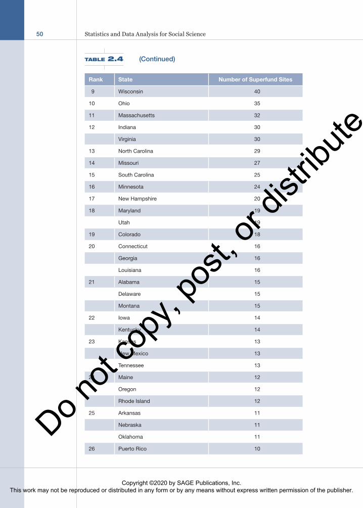
Table 2.4 was taken from the website http://scorecard.org on November 12, 2008. It ranks each state by the number of Superfund sites that were considered either “final” or “proposed” between 1993 and 2004. You can use the website to help assess the level of toxic contamination in your community.
Table 2.4 lists only sites that are either final or proposed and does not include all Superfund sites. A more complete list also includes those that are listed as deleted. In general, deleted sites are those that have been cleaned up. Including deleted sites gives us a better sense of the total hazards that a state has faced over time.
Using data collected directly from the EPA website on November 13, 2008, we see that each of the 1,650 sites falls into one and only one of these three attributes. Therefore, the variable is operationalized in a way that its attributes are both col-lectively exhaustive and mutually exclusive. By counting the number of sites in each attribute, we can quickly and easily describe the distribution of Superfund sites in Table 2.5.
Rank State Number of Superfund Sites
Vermont 10
27 Arizona 9
Idaho 9
West Virginia 9
28 Alaska 6
29 Mississippi 5
30 Hawaii 3
31 Guam 2
South Dakota 2
Virgin Islands 2
Wyoming 2
32 District of Columbia 1
Nevada 1
There is limited information about many potentially significant sources of contamination. Scorecard’s profiles of hazardous waste sites are limited to final and proposed sites on the National Priority List and are derived from multiple sources dating from 1993 to 2004.
Source: Data from the U.S. Environmental Protection Agency.
National Priorities List Statustable 2.5
Frequency Percent Valid Percent Cumulative Percent
Valid Deleted 330 20.0 20.0 20.0
Final 1,257 76.2 76.2 96.2
Proposed 63 3.8 3.8 100.0
Total 1,650 100.0 100.0
Source: Data from the U.S. Environmental Protection Agency.
52 Statistics and Data Analysis for Social Science
Status of Superfund Sitesfigure 2.4
63 Proposed
330 Deleted
1,257 Final
Status of Superfund Sitesfigure 2.3
Deleted Final0
200
400
600
800
1,000
1,200
1,400
Proposed
As you can see in the bar chart in Figure 2.3, the height of each bar corresponds to its frequency (or valid percent). Bar charts are a good way of displaying data at the nominal and ordinal levels. The data labels at the top of each bar can represent frequencies, percentages, or both depending on what you would like to display. In this case, they show frequencies. The same data are shown in the form of a pie chart in Figure 2.4. The relative size of each pie slice represents either the number of cases or the valid percent of cases.
Site Status is operationalized as a nominal variable because the attributes can-not be rank-ordered from high to low. It is often tempting to think of some nominal variables as ordinal variables. In the case of Site Status, for example, some might claim that we can rank the attributes because active sites pose a greater threat than do deleted or proposed sites. Two problems arise with this kind of logic. First, a proposed site could actually pose a much greater threat than an active site. Second,
Source: Data from the U.S. Environmental Protection Agency.
Source: Data from the U.S. Environmental Protection Agency.
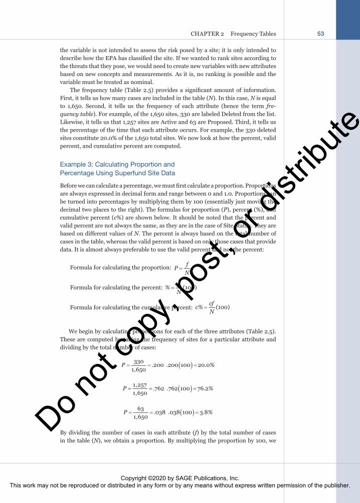
the variable is not intended to assess the risk posed by a site; it is only intended to describe how the EPA has classified the site. If we wanted to rank sites according to the threats that they pose, we would need to create new variables with new attributes based on new concepts and measurements. As it is, no ranking is possible and the variable must be treated as nominal.
The frequency table (Table 2.5) provides a significant amount of information. First, it tells us how many cases are included in the table (N). In this case, N is equal to 1,650. Second, it tells us the frequency of each attribute (hence the term fre-quency table). For example, of the 1,650 sites, 330 are labeled Deleted from the list. Likewise, it tells us that 1,257 sites are Active and 63 are Proposed. Third, it tells us the percentage of the time that each attribute occurs. For example, the 330 deleted sites constitute 20.0% of the 1,650 total sites. We now look at how the percent, valid percent, and cumulative percent are computed.
Example 3: Calculating Proportion and Percentage Using Superfund Site Data
Before we can calculate a percentage, we must first calculate a proportion. Proportions are always expressed in decimal form and range between 0 and 1.0. Proportions can be turned into percentages by multiplying them by 100 (essentially just moving the decimal two places to the right). The formulas for proportion (P), percent (%), and cumulative percent (c%) are shown below. It should be noted that the percent and valid percent are not always the same, as they are in the case of Site Status. They are based on different values of N. The percent is always based on the total number of cases in the table, whereas the valid percent is based on only those cases that provide data. It is almost always preferable to use the valid percent and not the percent:
Formula for calculating the proportion: P fN
=
Formula for calculating the percent: % =fN
( )100
Formula for calculating the cumulative percent: c cfN
% = ( )100
We begin by calculating proportions for each of the three attributes (Table 2.5). These are computed by taking the frequency of sites for a particular attribute and dividing by the total number of cases:
P = = =( )3301 650
200 200 100 20 0,
. . . %
P = = ( ) =1 2571 650
762 762 100 76 2,,
. . . %
P = ( )= =63
1 650038 038 100 3 8
,. . . %
By dividing the number of cases in each attribute (f) by the total number of cases in the table (N), we obtain a proportion. By multiplying the proportion by 100, we
54 Statistics and Data Analysis for Social Science
obtain a percent. For example, the proportion of cases that are deleted is .200 and the percent of cases that are deleted is 20.0%.
In Table 2.5, you can see that next to the Percent column in the text is a Valid Percent column. In this particular table, the two columns are the same; however, this is not always the case. Often frequency tables contain what are called “missing” cases. An example of a table with missing cases is presented later.
The final column in the frequency table is called the Cumulative Percent column. The Cumulative Percent column offers a running total of the Frequency column. For example, you can see that the first cumulative percent value is 20.0%. The next is 96.2%. This value is based on a cumulative frequency (cf) and is obtained by adding the frequency for deleted to the frequency for active and dividing by N. For example:
c% ,,
. %=+
=300 1 257
1 650100 96 2( )
This means that 96.2% of all Superfund sites are either deleted or active.
NOW YOU TRY IT 2.2
Suppose you are doing a study of student inte-gration into social life on campus and want to find out what percent of students live on cam-pus. Using a survey research method, you ask
students about their sex, class standing, and what percent of their time they spend on campus. You then test out your questionnaire on a group of students in a dining hall and find the following:
Respondent # Sex Class Standing Time on Campus
1 Male Freshman 90
2 Male Junior 75
3 Female Junior 60
4 Female Sophomore 85
5 Female Freshman 95
6 Male Senior 50
7 Female Junior 70
8 Female Senior 60
9 Male Sophomore 90
10 Female Junior 70
Using the data from the test of your ques-tionnaire, construct a frequency table for the variable sex. Be sure to include value labels,
frequencies, percents, valid percents, and cumulative percents. It is also standard proce-dure to include a title with each table.
For this example, the NPL sites are organized into four groups based on the number of sites in each state. Our unit of analysis is no longer waste sites. The unit of analysis is now states because we are looking at characteristics of states, not characteristics of waste sites. Therefore, the data presented here is ecological data. Territories were removed from the data, and only the 50 U.S. states and the District of Columbia are included. This reduces the overall number of cases to 51, so that N = 51. It also reduces the number of sites in these states from 1,650 to 1,616 because some geo-graphic regions have been left out of the analysis.
Example 4: Analyzing Superfund Site Data by State
The states are now organized into four groups (attributes) based on the number of waste sites. The first group of states consists of those that contain anywhere from 0 to 15 Superfund sites. The second group of states consists of those that contain any-where from 16 to 30 Superfund sites. The third group of states consists of those that contain anywhere from 31 to 45 Superfund sites. The final group of states consists of those that contain 46 or more sites. Table 2.6 shows the distribution, and Figure 2.5 shows the distribution in the form of a bar chart.
Frequency of Superfund Sitesfigure 2.5
0 to 15 Sites02468
101214161820
16 to 30 Sites 31 to 45 Sites 46 or More Sites
Frequency of Superfund Sitestable 2.6
Frequency Percent Valid Percent Cumulative Percent
Valid 0 to 15 sites 18 35.3 35.3 35.3
16 to 30 sites 16 31.4 31.4 66.7
31 to 45 sites 7 13.7 13.7 80.4
46 or more sites 10 19.6 19.6 100.0
Total 51 100.0 100.0
Source: Data from the U.S. Environmental Protection Agency.
Source: Data from the U.S. Environmental Protection Agency.
56 Statistics and Data Analysis for Social Science
Table 2.6 indicates that 18 states have between 0 and 15 sites, 16 states have between 16 and 30 sites, 7 states have between 31 and 45 sites, and 10 states have 46 or more sites. The attributes are mutually exclusive and collectively exhaustive. As you can see, the columns in the frequency table are the same as they were for the pre-vious one. They are the same for all frequency tables generated by SPSS for Windows.
This variable is ordinal, although it is easy to be fooled into thinking that it is interval/ratio because the attributes are represented as ranges of numbers. Here is the justification. When looking at the attributes in Table 2.6, it is possible to say that those states with 31 to 45 sites have more than those states with 16 to 30 sites. On the other hand, we cannot tell exactly how many more sites are in a state with 16 to 30 sites compared with a state with 0 to 15 sites. It could be 1 additional site, it could be 30 additional sites, or it could be anything in between. The point is that we just don’t know, nor can we tell from the table. Therefore, we can only say that one state has more or less sites than another state, thereby making the variable ordinal. Because we are unable to determine the exact difference in the frequency of sites between the two states, the variable is ordinal.
This is called grouped data, and it is important to realize that just because the table has numbers for the attributes does not make it an interval/ratio variable.
All percentages are calculated using the same methods and formulas that were used to calculate them in the previous table using the formula for percentage (%):
% =fN
( )100
0 to 15 sites: % .= =1851
100 35 3( ) . Therefore, 35.3% of all states contain 0 to 15
Superfund sites.
16 to 30 sites: % .= =1651
100 31 4( ) . Therefore, 31.4% of all states contain 16 to 30
Superfund sites.
31 to 45 sites: % .= =751
100 13 7( ) . Therefore, 13.7% of all states contain 31 to 45
Superfund sites.
46 or more sites: % .= =1051
100 19 6( ) . Therefore, 19.6% of all states contain 46 or
more Superfund sites.
The Cumulative Percent column is more applicable for tables with ordinal variables. Cumulative percents are calculated using the following formula:
c cfN
% = ( )100
0 to 15 sites: c% .= =1851
100 35 3( ) . Therefore, 35.3% of all states contain 0 to 15
Superfund sites.
0 to 30 sites: c% .=+
=18 16
51100 66 7( ) . Therefore, 66.7% of all states contain 0
51100 80 4( ) . Therefore, 80.4% of all states contain
0 to 45 Superfund sites.
0 to 46 or more sites: c% .=+ + +
=18 16 7 10
51100 100 0( ) . Therefore, 100.0% of
all states contain 0 to 46 or more Superfund sites.
NOW YOU TRY IT 2.3
Using the preliminary data from your study of integration into campus social life, construct a frequency table for the variable class standing.
Be sure to include value labels, frequencies, percents, valid percents, and cumulative percents.
Respondent # Sex Class Standing Time on Campus
1 Male Freshman 90
2 Male Junior 75
3 Female Junior 60
4 Female Sophomore 85
5 Female Freshman 95
6 Male Senior 50
7 Female Junior 70
8 Female Senior 60
9 Male Sophomore 90
10 Female Junior 70
FREQUENCY TABLE FOR AN INTERVAL/RATIO VARIABLE
For this example, the NPL sites are organized by states and the District of Columbia (hence N = 51 instead of 50). Unlike the last example, the states are not grouped into categories based on the number of sites they contain. Yet we use the same formula for percent (%) and cumulative percent (c%) that we used for the previous tables:
58 Statistics and Data Analysis for Social Science
Example 5: Looking at Interval/Ratio Variables in Superfund Site Data
Table 2.7 indicates that two states have 1 Superfund site, one state has 1 site, and so on:
For 1 Superfund site: % .= =2
51100 3 9states ( ) . Therefore, 3.9% of all states have
1 Superfund site.
For 2 Superfund sites: % .= =1
51100 2 0state ( ) . Therefore, 2.0% of all states have
2 Superfund sites.
For 3 Superfund sites: % .= =1
51100 2 0state ( ) . Therefore, 2.0% of all states have
3 Superfund sites.
This process is repeated for each row in the table, so that each row consists of a value, frequency, percent, valid percent, and cumulative percent. Cumulative percents are now discussed.
The Cumulative Percent column is particularly useful for tables with interval/ratio variables. For example, if we want to know how many states have 4 or fewer Superfund sites, we look at the first column of Table 2.7 and identify those rows in the table that indicate 0 to 4 sites. When we move across the table, we find that the cumulative percent for 4 sites is 11.8%. This means that 11.8% of all states have 4 or fewer Superfund sites.
The Cumulative Percent column is best thought of as a running total of the Valid Percent column. It is important to realize, however, that the calculation of cumula-tive percents cannot be accomplished by adding up the valid percents. The reason for this is that it is possible that the rounding error in each valid percent equation could be compounded when they are summed. The way to get around the possibil-ity of compounded rounding error is to base the cumulative percent on cumulative frequencies. Using our example of states with 0 to 4 Superfund sites, we find that two
60 Statistics and Data Analysis for Social Science
Constructing Frequency Tables From Raw Data
Constructing frequency tables is a relatively simple process, but it requires careful attention to detail. Imagine that you walk into a typical classroom on a college cam-pus and ask each student to tell you his or her age. You get the following results:
The following sections demonstrate how these data are organized into a frequency table.
The Frequency Column. Taking these 20 cases of raw data and organizing them into a frequency table begins with making a table with two columns, one that lists the attributes of our variable (the ages that respondents indicated) and one that lists the frequency (f) that each age occurred (Table 2.8).
The Percent Column. To calculate the Percent column, we divide each frequency by N to obtain the proportion. Then we multiply the proportion by 100 to obtain the percent:
Number of Sites Frequency Percent Valid Percent Cumulative Percent
36 1 2.0 2.0 74.5
40 1 2.0 2.0 76.5
44 1 2.0 2.0 78.4
45 1 2.0 2.0 80.4
46 1 2.0 2.0 82.4
51 1 2.0 2.0 84.3
59 1 2.0 2.0 86.3
65 1 2.0 2.0 88.2
72 1 2.0 2.0 90.2
84 1 2.0 2.0 92.2
107 1 2.0 2.0 94.1
110 1 2.0 2.0 96.1
123 1 2.0 2.0 98.0
140 1 2.0 2.0 100.0
Total 51 100.0 100.0
Source: Data from the U.S. Environmental Protection Agency.
62 Statistics and Data Analysis for Social Science
17 120
100 5 0: ( )% . %= =
18 220
100 10 0: ( )% . %= =
19 420
100 20 0: ( )% . %= =
20 720
100 35 0: ( )% . %= =
21 320
100 15 0: ( )% . %= =
22 120
100 5 0: ( )% . %= =
24 120
100 5 0: ( )% . %= =
25 120
100 5 0: ( )% . %= =
We can then add the percentages to the Percent column in Table 2.9.
table 2.9
Age Frequency Percent
17 1 5.0
18 2 10.0
19 4 20.0
20 7 35.0
21 3 15.0
22 1 5.0
24 1 5.0
25 1 5.0
Total 20 100.0
The Cumulative Percent Column. Finally, we can create a Cumulative Percent column (c%) using cumulative frequencies (cf). Remember, the Cumulative Percent column summarizes data up to a given point in a frequency table. For example, we may want to know what percent of respondents are younger than 20 years. To calculate this, we need to find out how many respondents are younger than 20 years (which, in this case, is another way of asking for the cumulative frequency for 17-, 18-, and 19-year-olds). We do this as follows:
These values can now be added as another column in Table 2.10.
table 2.10
Age Frequency Percent Cumulative Percent
17 1 5.0 5.0
18 2 10.0 15.0
19 4 20.0 35.0
20 7 35.0 70.0
21 3 15.0 85.0
22 1 5.0 90.0
24 1 5.0 95.0
25 1 5.0 100.0
Total 20 100.0
Getting back to our earlier question, because there are one 17-year-old, two 18-year-olds, and four 19-year-olds, the cumulative frequency is 1 + 2 + 4 = 7. Therefore, the cumulative percent for 19-year-olds is (7 ÷ 20)(100) = 35.0%. We can now state that 35.0% of the students in our sample are younger than 20 years old.
64 Statistics and Data Analysis for Social Science
How Satisfied Are You With Your College Experience?table 2.11
Frequency (f )
Very satisfied 342
Somewhat satisfied 116
Not satisfied 42
Total 500
INTEGRATING TECHNOLOGY
In its annual Human Development Report, the United Nations gathers tremendous amounts of data from countries all over the world and makes these data available to the public via the Internet. Data can be viewed online or downloaded into Microsoft Excel files (which can then be saved in a variety of formats that most statistics software programs can read). These include data on literacy rates, health care, carbon dioxide emissions, gender discrimination, vital statistics (births, deaths), and income inequality, among many others. Follow this link for a recent report: http://hdr.undp.org/en/
One interesting exercise is to sort countries from lowest to highest by different variables to see what other countries have similar characteristics. While we in the United States tend to compare the United States with many Western European countries, you may be surprised to see that in terms of income inequality, the United States is more similar to many nations with much less developed economies.
Example 6: Student Satisfaction With Their College Environment
Here is another example of how to use frequency tables. Suppose that for a class project, you are asked to survey students on their overall satisfaction with the overall quality of their college environment. You sample 500 students, asking them if they are “very satisfied,” “somewhat satisfied,” or “not satisfied.” You are now faced with the task of sifting through 500 sheets of paper with your respondents’ responses in an attempt to figure out how they tend to feel about their college experience. This is a good time to consider constructing a frequency table!
To construct a frequency table, tally the responses for each of the three attributes. Suppose you find that 342 respondents are “very satisfied,” 116 are “somewhat satis-fied,” and 42 are “not satisfied.” You can now summarize your responses in a table format like the one in Table 2.11.
The next task is to display these data in the form of percentages instead of fre-quencies. For example, if someone asked how satisfied students are with their college experience, you could answer that 342 of 500 are very satisfied. This kind of answer, however, is not easy to interpret. It makes more sense to state our response as a per-centage because it summarizes our findings by putting them into a format that is easy to understand and communicate.
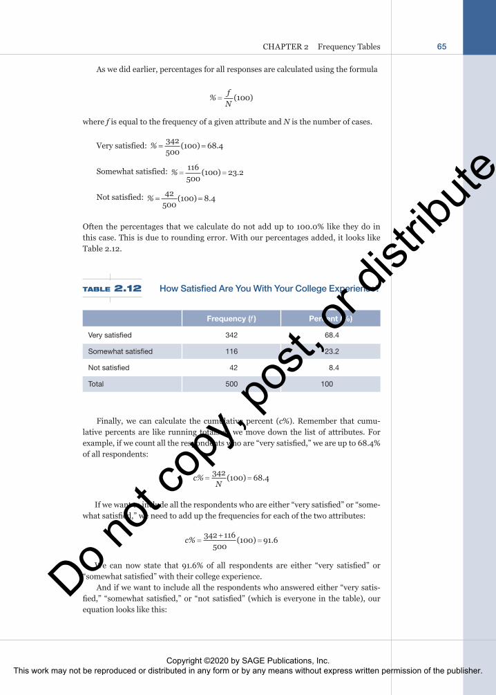
As we did earlier, percentages for all responses are calculated using the formula
% =fN
( )100
where f is equal to the frequency of a given attribute and N is the number of cases.
Very satisfied: % .= =342500
100 68 4( )
Somewhat satisfied: % .= =116500
100 23 2( )
Not satisfied: % .= =42
500100 8 4( )
Often the percentages that we calculate do not add up to 100.0% like they do in this case. This is due to rounding error. With our percentages added, it looks like Table 2.12.
How Satisfied Are You With Your College Experience?table 2.12
Frequency (f ) Percent (%)
Very satisfied 342 68.4
Somewhat satisfied 116 23.2
Not satisfied 42 8.4
Total 500 100
Finally, we can calculate the cumulative percent (c%). Remember that cumu-lative percents are like running totals as we move down the list of attributes. For example, if we count all the respondents who are “very satisfied,” we are up to 68.4% of all respondents:
cN
% .= =342 100 68 4( )
If we want to include all the respondents who are either “very satisfied” or “some-what satisfied,” we need to add up the frequencies for each of the two attributes:
c% .=+
=342 116
500100 91 6( )
We can now state that 91.6% of all respondents are either “very satisfied” or “somewhat satisfied” with their college experience.
And if we want to include all the respondents who answered either “very satis-fied,” “somewhat satisfied,” or “not satisfied” (which is everyone in the table), our equation looks like this:
66 Statistics and Data Analysis for Social Science
c% .=+ +
=342 116 42
500100 100 0( )
Of course, this is 100% of all the cases. It is tempting for many students to calcu-late the cumulative percent (c%) by adding percentages from the Percent column, for example, 68.4 + 23.2%. However, this is risky because of the potential for rounding error in each percent to add up to a more significant rounding error when we com-bine the percentages. When the Cumulative Percent column is added, it looks like Table 2.13.
How Satisfied Are You With Your College Experience?table 2.13
Frequency (f ) Percent (%) Cumulative Percent
Very satisfied 342 68.4 68.4
Somewhat satisfied 116 23.2 91.6
Not satisfied 42 8.4 100.0
Total 500 100.0
It is common for social scientists to use statistical software packages to enter and analyze their data. A common one is called SPSS for Windows. SPSS stands for Statistical Program for the Social Sciences. It is used to generate many of the tables and charts presented in this book. Table 2.14 is based on the same data as the one above and was generated using SPSS for Windows.
How Satisfied Are You With Your College Experience?table 2.14
Frequency Percent Valid Percent Cumulative Percent
Valid Very satisfied 342 68.4 68.4 68.4
Somewhat satisfied 116 23.2 23.2 91.6
Not satisfied 42 8.4 8.4 100.0
Total 500 100.0 100.0
The table is neat, orderly, and easily interpreted. Best of all, many statistical soft-ware packages automatically generate these tables with just a few clicks of the mouse. The chart in Figure 2.6 provides the same information as the table, yet it does so in a way that emphasizes the trend that most students are very satisfied.
STATISTICAL USES AND MISUSESBeware of “mind-blowing” statistics! Newspapers, magazines, and other media outlets often report on rapid change in society. For example, we may read in the local newspaper that our community’s murder rate has jumped by 50% relative to a year ago. This may or may not be cause for concern. If the number of murders at this time last year was two, then a 50% increase means that our commu-nity has had three murders this year. An increase from two to three is not much of an increase (at least in most cities), and to report that as a 50% increase, while statistically true, is to mislead the consumers of these statistics by making them think the problem is bigger than it really is.
Another problem that can arise with per-centages is related to the social and geographic specificity of statistics. Often statistics that are intended to represent an entire society represent only a portion of the population. For example, we may read that the number of murders so far this year is double the number of murders from
this time last year. This does not, however, mean that everyone is at twice the risk of being mur-dered. It may be that the majority of all murders take place in cities with populations of 250,000 or more. (I should state that this is only a hypo-thetical example and that I do not actually know where most murders take place.) Therefore, it is possible that the overall increase in murders in these urban areas is rising and causing the nationwide murder rate to rise, while other types of communities could be seeing declines in their murder rates.
The same could be true with any kind of social phenomena—child abductions, runaways, rapes, and so on. It is important to know what kinds of questions to ask when we hear these “mind-blowing” statistics. What are the frequencies on which these statistics are based? To what populations can these statistics be generalized? And maybe most important, who has an interest in reporting these kinds of statistics?
Satisfaction With College Experiencefigure 2.6
Very Satis�ed
400
350
300
250
200
150
100
50
0Somewhat Satis�ed Not Satis�ed
Frequency Tables and Missing Cases. To recap a discussion from earlier, be aware of which percent you are reading in a table. As you can see by comparing Tables 2.13 and 2.14, the one generated by SPSS for Windows provides an additional column that distinguishes valid percent from percent. The difference between percent and valid percent is important. While Percent columns are based on the total number of cases in the data, Valid Percent columns are based on only the cases that provided data for the variable being analyzed. In other words, the value of N is often different
The Valid Percent column values are based on an N of 1,517, which includes only those respondents who provided data for the table. The formula for the valid percent is
Valid % ,,
.= =1 3302 993
100 87 7( )
It is preferable to use the valid percent over the percent because missing cases really don’t tell us anything. Would you feel comfortable claiming that 87.7% of the sample has ever worked as long as one year when 2,988 (66.3%) of those people did not provide any data at all? Of course not! That is why we use the valid percent.
You can see that Table 2.15 indicates that 2,993 cases are missing. Cases may be missing for a variety of reasons. For example, in this table, 2,988 respondents indicated that the question was not applicable to them (we don’t know why) and that another 5 respondents did not answer the question (again, we do not know why).
Table 2.16 is a frequency table for a variable that describes respondents’ political views. The first column lists the attributes of the variable think of self as liberal or conservative. The frequency column shows the number of respondents who answered “extremely liberal,” “liberal,” and so on. The Percent column shows the percent of all 2,867 respondents who were presented with the questionnaire. The Valid Percent col-umn shows only the percent of responses based on the number of valid responses (N = 2,756). In other words, 2,867 respondents were included in the study, yet only 2,756 respondents provided valid responses. Of the 111 respondents who did not provide data, 81 did not know what to answer and 30 indicated that the questionnaire item was not applicable to them. Because these 111 respondents provide no data, they should be excluded from the analysis. Finally, the Cumulative Percent column, which is based on only those valid cases providing data, represents a “running total” of the data from one row to the next.
Do You Think of Yourself as Liberal or Conservative?table 2.16
Frequency Percent Valid Percent Cumulative Percent
Valid Extremely liberal 136 4.7 4.9 4.9
Liberal 350 12.2 12.7 17.6
Slightly liberal 310 10.8 11.2 28.9
Moderate 1,032 36.0 37.4 66.3
Slightly conservative 382 13.3 13.9 80.2
Conservative 426 14.9 15.5 95.6
Extremely conservative 120 4.2 4.4 100.0
Total 2,756 96.1 100.0
Missing Don’t know 81 2.8
Not applicable 30 1.0
Total 111 3.9
Total 2,867 100.0
Source: Data from the National Opinion Research Center, General Social Survey.
70 Statistics and Data Analysis for Social Science
In general, missing cases are left out of all analyses. Often students see this as problematic, but it is important to remember that the data are missing and, there-fore, do not exist. For whatever reason, respondents chose not to give us that infor-mation or the question did not apply to them. Therefore, it is common practice to exclude missing cases. The Valid Percent and Cumulative Percent columns in the frequency table are calculated on the basis of no missing cases. In Table 2.16, you can see that the response “extremely liberal” has a percent of 4.7 and a valid percent of 4.9. We see that 136 respondents are extremely liberal. This represents 4.7% of the 2,867 respondents surveyed and 4.9% of the 2,756 respondents who answered the question. The difference is this: The percent is based on 2,867 cases, and the valid percent is based on 2,756 cases. If you feel that it is important to include missing cases, read the Percent column instead of the Valid Percent column. A graphic repre-sentation (in this case it is a pie chart) of Table 2.16 is shown in Figure 2.8.
Think of Self as Liberal or Conservative?figure 2.8
Extremely Liberal
Slightly Liberal
Moderate
Slightly Conservative
Conservative
Extremely Conservative
Liberal
EYE ON THE APPLIEDDESCRIBING AND SUMMARIZING DATA
Frequency tables may be the most commonly used method of summarizing and communicating large amounts of data. They are much more common than you might think. A quick test of this can be done using a USA Today newspaper or a Time or Newsweek magazine. Take a few minutes and flip through the pages of one of these publications, making note of the number of pie charts and bar graphs you see. Each pie chart and bar graph is based on a frequency table. A wide array of computer software programs enable their users to quickly change the format in which data are presented from a table, which is understood by those trained to read tables, to graphic forms, which most people can easily understand. The example below shows the same data in three different formats.
Source: Data from the National Opinion Research Center, General Social Survey.
This chapter was all about how to organize data so that we can more easily summarize results, identify trends, and communicate results with others. A popular way to summarize data is by using frequency tables. Fre-quency tables show the distribution of cases across the attributes of a single variable and make extensive use of both frequencies and percentages (percent and valid percent). In addition to tables, this chapter empha-sized the presentation of data in visual forms such as charts (pie charts, bar charts). As a general rule, pie charts are used for nominal variables, while bar charts are used for either nominal or ordinal variables.
CHAPTER EXERCISES
Use Table 2.17 to answer the subsequent questions.
Religious Preferencetable 2.17
Frequency Percent Valid Percent Cumulative Percent
Valid Protestant 953 63.5 63.9 63.9
Catholic 333 22.2 22.3 86.2
Jewish 31 2.1 2.1 88.3
None 140 9.3 9.4 97.7
Other 35 2.3 2.3 100.0
Total 1,492 99.5 100.0
Missing DK 1 .1
NA 7 .5
Total 8 .5
Total 1,500 100.0
Source: Data from the National Opinion Research Center, General Social Survey.
Note: DK, don’t know; NA, no answer.
1. how many respondents provided data?
2. how many missing cases are there?
3. how many respondents are Protestant?
4. What percent of respondents are Protestant?
5. Is the variable nominal, ordinal, or interval/ratio?
6. What proportion of respondents are Catholic?
7. What proportion of respondents are Jewish?
8. What percent of respondents are either Protestant or Catholic?
Use Table 2.18 to answer the subsequent questions.
10. Is the variable nominal, ordinal, or interval/ratio?
11. how many respondents provided data for this table?
12. How many respondents walked to class?
13. What proportion of respondents walked to class?
14. What percent of respondents walked to class?
15. What percent of respondents do not take public transportation?
Use the frequencies in Table 2.19 to fill in the Percent, Valid Percent, and Cumulative Percent columns. Then use the table to answer the subsequent questions.
How Do You Get to Class?table 2.18
Mode of Transportation Frequency (f )
Car 37
Public transportation 18
Walk 28
Bike 12
Other 20
Total 115
Do You Think of Yourself as Liberal or Conservative?table 2.19
Frequency Percent Valid Percent Cumulative Percent
Valid Extremely liberal 139
Liberal 524
Slightly liberal 517
Moderate 1,683
Slightly conservative 618
Conservative 685
Extremely conservative 167
Total 4,333
Missing Don’t know 154
Not applicable 23
Total 177
Total 4,510 100.0
Source: Data from the National Opinion Research Center, General Social Survey.
16. Is this variable nominal, ordinal, or interval/ratio?
17. how many attributes does this variable have?
18. how many respondents provided data (what is N equal to)?
19. What percent of respondents are slightly conservative?
20. What percent of respondents are more liberal than slightly liberal?
IN-CLASS EXERCISES
In total, 23 college students taking statistics were surveyed. Each student responded to four questions. The results are shown in Tables 2.20 to 2.23. Use the frequency tables to answer Questions 1 to 14.
Is Respondent Graduating This Semester?table 2.20
Frequency Percent Valid Percent Cumulative Percent
Valid Yes 15 65.2 65.2 65.2
No 8 34.8 34.8 100.0
Total 23 100.0 100.0
How Worried Is Respondent About Statistics?table 2.21
Frequency Percent Valid Percent Cumulative Percent
Valid Not very 11 47.8 47.8 47.8
Somewhat 8 34.8 34.8 82.6
Very 4 17.4 17.4 100.0
Total 23 100.0 100.0
Does Respondent Own a Computer?table 2.22
Frequency Percent Valid Percent Cumulative Percent