Fresnel diffraction from curved fiber snippets with application to fiber diameter measurement Monty Glass Fiber curvature is examined for its effect on apparent measured fiber diameter in a double-diffraction- based instrument that is in widespread use in the wool industry. The development uses a two- dimensional Fresnel diffraction model. The magnitude of the effect is studied for 2-mm-long snippets of various diameters from 8 to 50 μm and with radii of curvature of 1 m 1straight2, 600 μm, 280 μm, 200 μm, and 160 μm. The two-dimensional Fresnel model gives rise to deeply nested vector integrations that make computations with a straightforward approach exceedingly time consuming and impractical. A number of simplifying techniques are used to facilitate and speed up the numerical computations, thereby permitting investigations to be carried out on a personal computer. Key words: Fresnel diffraction, double diffraction, fiber diameter, Gaussian beams, Laserscan. 1. Introduction The Laserscan is a laser-based instrument used to measure the distribution of wool fiber diameters within a sample of fiber snippets. The device in its present form relies on a light-scattering technique and was first described by Lynch and Michie. 1,2 The instrument is capable of accurately measuring fiber diameters in the typical range of 5–150 μm and is now in widespread use in the wool industry. A full and precise treatment of all the phenomena involved in light scattering from wool fibers would have to resort to the solution of Maxwell’s equations and would therefore take account of both surface geometry through the boundary conditions and also bulk properties by means of the complex refractive index. Fortunately, when the diameter of the scat- tering object 1wool fiber in this case2 is large com- pared with the wavelength of the incident light 1the size parameter, pd@l, is ,50 for a 10-μm-diameter fiber and red laser light2, the scattered light in the immediate vicinity of the geometric shadow is domi- nated by diffraction. 3 Although diffraction theory does not generally supply information with regard to polarization effects, the intensity and spacing of fringes can be accurately predicted by replacement of the wool fiber with an opaque diffracting strip whose width is equal to the fiber diameter. A simplified schematic diagram of the Laserscan measurement system is shown in Fig. 1. The beam from a helium–neon laser illuminates a round pin- hole that effectively resizes the beam at the measure- ment cell plane. Light emerges from the pinhole in a characteristic Airy diffraction ring pattern and passes through a glass-walled measurement flow cell, through which flows a dilute slurry of 1.2 mm long2 fiber snippets in isopropanol and 8% water by volume. Some of the light is split off from the laser beam before the cell and is monitored at the refer- ence detector for changes in laser power. A fiber in the cell, on passing through the beam, scatters and diffracts the laser light. The measure- ment detector catches some of the diffracted light from the wool fiber, and the drop in power, or the degree of beam occlusion seen by the detector, gives a direct measure of fiber diameter. Some of the light emerging from the cell is split off and diverted onto the face of an optical fiber discriminator, which is used to discriminate against invalid measurements such as dirt, fragments, snippets not fully intersect- ing the beam, and double or multiple fibers. The instrument is calibrated by the measurement of a number of known standard fiber samples whose diameter distributions have been previously deter- mined by the use of projection microscopy. A sample of crimped wool, prepared for measure- ment in a pinhole-apertured expanding beam Laser- The author is with the Division of Wool Technology, Sydney Laboratory, Commonwealth Scientific and Industrial Research Organization, P.O. Box 7, Ryde, New South Wales 2112, Australia. Received 26 June 1995; revised manuscript received 3 August 1995. 1 April 1996 @ Vol. 35, No. 10 @ APPLIED OPTICS 1605
Transcript
Fresnel diffraction from curved fiber snippetswith application to fiber diameter measurement
Monty Glass
Fiber curvature is examined for its effect on apparent measured fiber diameter in a double-diffraction-based instrument that is in widespread use in the wool industry. The development uses a two-dimensional Fresnel diffraction model. The magnitude of the effect is studied for 2-mm-long snippetsof various diameters from 8 to 50 µm and with radii of curvature of 1 m 1straight2, 600 µm, 280 µm, 200µm, and 160 µm. The two-dimensional Fresnel model gives rise to deeply nested vector integrationsthat make computations with a straightforward approach exceedingly time consuming and impractical.A number of simplifying techniques are used to facilitate and speed up the numerical computations,thereby permitting investigations to be carried out on a personal computer.Key words: Fresnel diffraction, double diffraction, fiber diameter, Gaussian beams, Laserscan.
1. Introduction
The Laserscan is a laser-based instrument used tomeasure the distribution of wool fiber diameterswithin a sample of fiber snippets. The device in itspresent form relies on a light-scattering techniqueand was first described by Lynch andMichie.1,2 Theinstrument is capable of accurately measuring fiberdiameters in the typical range of 5–150 µm and isnow in widespread use in the wool industry.A full and precise treatment of all the phenomena
involved in light scattering from wool fibers wouldhave to resort to the solution of Maxwell’s equationsand would therefore take account of both surfacegeometry through the boundary conditions and alsobulk properties by means of the complex refractiveindex. Fortunately, when the diameter of the scat-tering object 1wool fiber in this case2 is large com-pared with the wavelength of the incident light 1thesize parameter, pd@l, is ,50 for a 10-µm-diameterfiber and red laser light2, the scattered light in theimmediate vicinity of the geometric shadow is domi-nated by diffraction.3 Although diffraction theorydoes not generally supply information with regard topolarization effects, the intensity and spacing offringes can be accurately predicted by replacement
The author is with the Division of Wool Technology, SydneyLaboratory, Commonwealth Scientific and Industrial ResearchOrganization, P.O. Box 7, Ryde, New SouthWales 2112,Australia.Received 26 June 1995; revised manuscript received 3 August
1995.
of the wool fiber with an opaque diffracting stripwhose width is equal to the fiber diameter.A simplified schematic diagram of the Laserscan
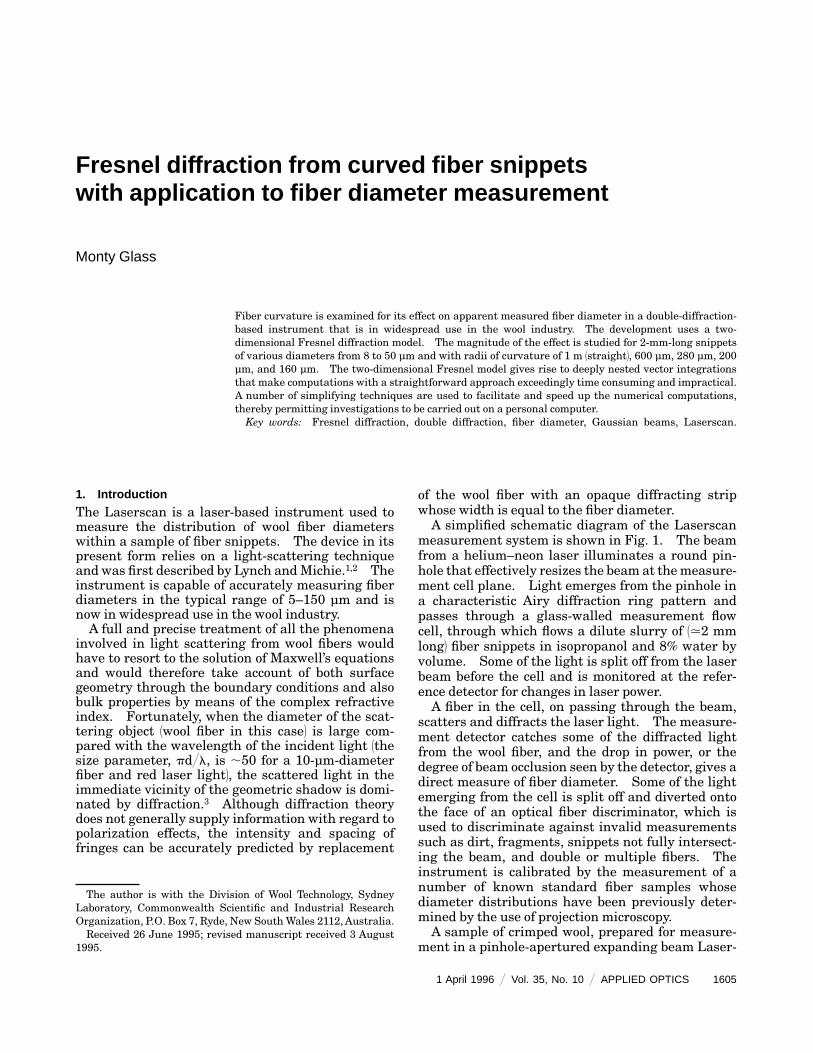
measurement system is shown in Fig. 1. The beamfrom a helium–neon laser illuminates a round pin-hole that effectively resizes the beam at themeasure-ment cell plane. Light emerges from the pinhole ina characteristic Airy diffraction ring pattern andpasses through a glass-walled measurement flowcell, through which flows a dilute slurry of 1.2 mmlong2 fiber snippets in isopropanol and 8% water byvolume. Some of the light is split off from the laserbeam before the cell and is monitored at the refer-ence detector for changes in laser power.A fiber in the cell, on passing through the beam,
scatters and diffracts the laser light. The measure-ment detector catches some of the diffracted lightfrom the wool fiber, and the drop in power, or thedegree of beam occlusion seen by the detector, gives adirect measure of fiber diameter. Some of the lightemerging from the cell is split off and diverted ontothe face of an optical fiber discriminator, which isused to discriminate against invalid measurementssuch as dirt, fragments, snippets not fully intersect-ing the beam, and double or multiple fibers. Theinstrument is calibrated by the measurement of anumber of known standard fiber samples whosediameter distributions have been previously deter-mined by the use of projection microscopy.A sample of crimped wool, prepared for measure-
scan 1EBL2, will inevitably contain curved fiber snip-pets. Viewed from the standpoint of a simplegeometric shadowingmodel 1seeAppendixA2, a curvedfiber snippet of given diameter will have a longerlength occluding the measurement beam than astraight snippet, and hence will show a highermeasured occlusion at the measurement detector.Although this geometrical opticsmodel gives a simplemethod of interpreting the effect caused by snippetcurvature, it ignores diffraction, and consequentlyestimates of the likely measurement differenceswith curved snippets are considerably in error.The optical phenomena that occur when a wire or
wool fiber traverses through the laser beam of anEBL are well described by a model based on diffrac-tion. An approximate one-dimensional diffractionanalysis of the EBL with infinitely long straightsnippets has been presented by Glass4 and Glass etal.5 Using a full two-dimensional diffraction model,this paper investigates the effect of snippet curva-ture and finite 2-mm snippet length on the diffrac-tion pattern at the detector and the consequentchanges in apparentmeasured diameter over straightsnippets.
2. Mathematical Model
A. Preliminary Considerations
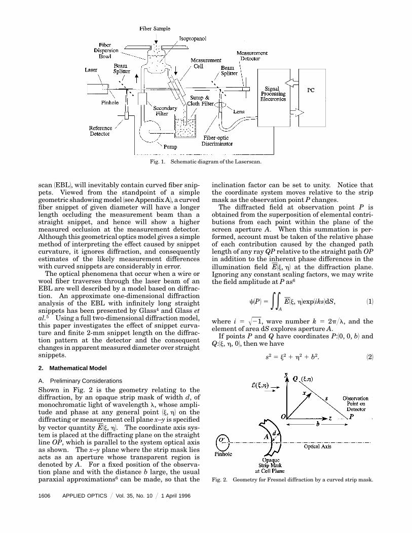
Shown in Fig. 2 is the geometry relating to thediffraction, by an opaque strip mask of width d, ofmonochromatic light of wavelength l, whose ampli-tude and phase at any general point 1j, h2 on thediffracting ormeasurement cell plane x–y is specifiedby vector quantity E1j, h2. The coordinate axis sys-tem is placed at the diffracting plane on the straightline OP, which is parallel to the system optical axisas shown. The x–y plane where the strip mask liesacts as an aperture whose transparent region isdenoted by A. For a fixed position of the observa-tion plane and with the distance b large, the usualparaxial approximations6 can be made, so that the
PLIED OPTICS @ Vol. 35, No. 10 @ 1 April 1996
inclination factor can be set to unity. Notice thatthe coordinate system moves relative to the stripmask as the observation point P changes.The diffracted field at observation point P is
obtained from the superposition of elemental contri-butions from each point within the plane of thescreen aperture A. When this summation is per-formed, account must be taken of the relative phaseof each contribution caused by the changed pathlength of any rayQP relative to the straight pathOPin addition to the inherent phase differences in theillumination field E1j, h2 at the diffraction plane.Ignoring any constant scaling factors, we may writethe field amplitude at P as6
c1P2 5 eeA
E1j, h2exp1iks2dS, 112
where i 5 Œ21, wave number k 5 2p@l, and theelement of area dS explores aperture A.If points P and Q have coordinates P:10, 0, b2 and
Q:1j, h, 02, then we have
s2 5 j2 1 h2 1 b2. 122
Fig. 2. Geometry for Fresnel diffraction by a curved strip mask.
Assuming that in the region of significant contribu-tion to the diffraction integral 112 the linear dimen-sions of the aperture are small in comparison with b,we may expand s as a power series in j@b and [email protected] terms up to the second order gives
s . b 1j2 1 h2
2b. 132
Now substituting relation 132 into Eq. 112 and againignoring any constant scaling factors, we see that thediffraction integral becomes
c1P2 5 eeA
E1j, h2exp3i p
lb1j2 1 h224djdh. 142
In its present form the diffraction integral of Eq. 142involves integration over the full transparent regionof the aperture at the diffraction plane denoted by A.In the previously treated one-dimensional model,4,5the Fresnel integrations to obtain the field at thedetector were in fact performed in this manner. Inthe present two-dimensional investigation this tech-nique is impractical, as the nested integrationsrequired to calculate the field at each point on thedetector make the calculation of detector power1involving another two-dimensional nested integra-tion2 computationally intensive and consequentlyenormously time consuming. A significant reduc-tion in computation time can be achieved by makinguse of Babinet’s principle6 to express the diffractionintegral as the difference of the unobstructed fieldseen by the detector and the field at the detector fromdiffraction by a region transparent only within theboundary of the strip mask. The field at the detec-tor may thus be written as
c1P2 5 eeA
5 eeunobstructedaperture
2 eeregion ofstrip mask
; c01P2 2 cm1P2, 152
where c01P2 is the unobstructed field on the detectorat point P and cm1P2 is the field on the detector atpoint P caused by a transparent strip mask at thediffraction plane.
B. Unobstructed Field at the Detector, c01P2, andCell, E1j, h2
For the purposes of this and the following section, itis convenient to use an alternative axis systemx8–y8–z8, as shown in Fig. 3, centered at O8 on theLaserscan optical axis at the pinhole. The pinholenow forms the diffraction aperture for computationof the unobstructed field at the detector, whichresults from truncation of the laser beam profile bythe pinhole. For any given point P:1x8, y8, z82 on the
detector and pointQ8:1j8, h8, h8, 02within the pinhole,distance s8 is
s82 5 1x8 2 j822 1 1 y8 2 h822 1 z82
5 1x82 1 y822 1 1j82 1 h8
22 2 21x8j8 1 y8h82 1 z82,
162
where
z8 5 a 1 b. 172
With the linear dimensions of the aperture small incomparison with z8, we may expand s8 as a powerseries in x8@z8, y8@z8, j8@z8, and h8@z8. Retainingterms up to the second order gives
s8 .1x82 1 y822
2z81
1j82 1 h8
22
2z82
1x8j8 1 y8h82
z81 z8. 182
In the case of the EBL, the circular pinhole ofdiameter D is illuminated by a laser wave frontwhose amplitude profile, with respect to the opticalaxis, is axisymmetric and Gaussian. It is thereforeprudent to change to the polar coordinates shown inFig. 3, as this brings about a considerable simplifica-tion in the mathematics. Substituting
j8 5 r cos u, 192
h8 5 r sin u, 1102
x8 5 r cos f, 1112
y8 5 r sin f 1122
into relation 182 then yields
s8 5r2
2z81
r2
2z82rr cos1u 2 f2
z81 z8. 1132
Noting that in polar coordinates an element ofarea dS 5 rdudr and denoting the illumination fieldat the pinhole by p 1r2, we find that the unobstructedfield at the detector resulting from diffraction at the
Fig. 3. Geometry for Fresnel diffraction by the Laserscan pin-hole.
Substituting from Eq. 1132 and ignoring the constantphase factor in z8, Eq. 1142 becomes
c01P2 5 exp1ikr2
2z8 2 e0D@2
p 1r2r exp1ikr2
2z8 2
3e0
2p
exp32 ikrr
z8cos1u2 f24dudr. 1152
Now for any fixed point P, angle f is also constant.Consequently the second integral of the expressionin Eq. 1152 can be written in terms of the zero-orderBessel function of the first kind,6 and
c01P2 5 exp1ikr2
2z8 2 e0D@2
p 1r2r exp1ikr2
2z8 22pJ01krrz8 2dr,
1162
as expected, is a function of r only. The illuminationfield on the pinhole or diffracting plane is Gaussianin amplitude and is given by7
p 1r, z082 5v0
vexp3if 1z082 2
r2
v21ikr2
2a0 4 , 1172
where v0 is the radius at the beam waist where theamplitude falls to 1@e of the centerline value, r is theradial distance from the beam centerline, and
v2 5 v0231 1 1z08zR 2
2
4 , 1182
a0 5 z0831 1 1zRz0822
4 , 1192
f 1z082 5 kz08 1 tan211z08zR 2 , 1202
with
zR 5pv0
2
l1212
being the Rayleigh range of the collimated waist.Equation 1172 represents a spherical wave whose
11@e2 size, at a distance z08 from the beam waist, is v
and whose wave-front radius of curvature is a0,whereas f 1z082 accounts for the phase of the wavefront relative to the beam waist. In the presentcase the laser beam waist is located on the frontresonator mirror of the laser. The first term with r2
in Eq. 1172 accounts for the Gaussian field profile,
whereas the second accounts for the approximatephase difference of the spherical wave front from aplanar surface. The beam may thus be thought ofas being represented by a point source at distance a0from the pinhole where the field amplitude is Gauss-ian. Substituting from Eq. 1172 for the field in Eq.1162 and ignoring any constant multipliers, we have
c01P2 5 exp1ikr2
2z8 2 e0D@2
r exp12 r2
v2 2J01krrz8 23 exp3ikr2
2 11z8 11
a024dr. 1222
Note that quantity r@z8 . U is the angle between thelineO8P and the z8 axis of Fig. 3.To obtain the field of illumination at the cell plane,
where the snippet or strip mask is located, oneproceeds as follows. If the coordinates of the axissystem centered on O at the cell plane are 1x8, y8, a2with respect to the x8–y8–z8 axis system centered atO8, then any general pointQ:1j, h2with respect to theaxis system centered at O will have coordinates1x8 1 j, y8 1 h2 with respect to the axes at O8.Equation 1222 can then be used to deduce E1j, h2 byputting z8 5 a and taking r2 5 1x8 1 j22 1 1 y8 1 h22.That is,
E1j, h2 5 exp5ik31x8 1 j22 1 1 y8 1 h224
2a 6 e0
D@2
r
3 exp12 r2
v22J05k31x8 1 j22 1 1 y8 1 h2241@2r
a 63 exp3ikr2
2 11a 11
a024dr. 1232
C. Phase and Amplitude Corrections
Throughout the above development, all constantamplitude and phase scaling factors associated withthe diffraction integrals have been ignored. Amorecareful treatment that uses Kirchhoff ’s diffractiontheory6 shows that the inclination factor in theFresnel diffraction integral used here has a phasefactor 2i associated with it. In the difference tech-nique used here, to compute the field at any point onthe detector Eq. 152 is used, with c01P2 coming fromEq. 1222 and E1j, h2 for integration in cm1P2 comingfrom Eq. 1232. Because of a double application of thediffraction integral to cm1P2, in order to maintainphase harmony, c01P2must be multiplied by i prior tosubstitution into Eq. 152.A number of unimportant amplitude factors have
also been omitted. Harmony between the ampli-tudes of c01P2 and cm1P2 was ensured by equalizationof the magnitude of the unobstructed field on theoptical centerline of the detector, computed from Eq.1222 and also directly from Eq. 142.
D. Curved Snippet Geometry
A number of different curved snippet geometricarrangements are possible for investigating the ef-fect of curvature on measurement in the Laserscan.The geometry chosen in this investigation was anattempt to look at the worst case. Provided theradius of curvature is greater than 2000@p 5 637µm, a 2000-µm long curved snippet can be unambigu-ously represented by an annular arc strip mask.For a snippet radius of curvature smaller than this,the curved snippet is represented by a strip maskcomprising a semicircular curved section plus hori-zontal end extensions, of the necessary length, tomake up a a total length of 2000 µm on the maskcenterline. In both cases the ends have been cutperpendicular to the snippet or mask centerline.The radii of curvature investigated were 1 m
1straight2, and 600, 280, 200, and 160 µm, whichcorrespond approximately to the different curlclasses, as defined by Dabbs et al.,8 seen by theLaserscan fiber-optic discriminator. Fiber diam-eters from 8 to 50 µmwere studied. Figure 4 shows,to scale, the various curved snippets studied, with asuperimposed circle representing the size of themeasurement laser beam, within the cell, at the firstminimum.It is necessary to determine the mathematical
boundary of the various curved masks in order toperform the integration for cm1P2 in Eq. 152. Figure51a2 shows the geometry in which the radius ofcurvature is greater than 637 µm and consequentlythe mask is an annular arc only. The boundaryequations are first determined with respect to thex8–y8 axes centered atO8 on the optical axis, and thenlater they are transformed to the mask diffractionintegral axes x–y, centered at O. The center of thecurved mask of width d is shown offset by an amountjoff from the y8 axis. If s is the radius of curvature ofthe mask centerline, then the radii of the inner andouter circular arcs are
respectively. Noting that consistent 1SI2 units mustbe used, we see that angle a of a radial line drawn tothe end of the curved mask as shown is
a 5 0.001@s, 1262
so that the distances from the x8 axis of the outer-most points on the inner and outer circular arcs are
hi,max8 5 si sin a, 1272
ho,max8 5 so sin a, 1282
respectively.For any given h8, we can now determine ji8 and jo8,
the inner and outer x8 values on the mask boundary,by using the equations for the inner and outer circlesand simple geometry in the region of the mask end.Such consideration shows that when 0h8 0 # hi,max8,
ji8 5 1si2 2 h8
221@2 2 s 1 joff ; 1292
when hi,max8 , 0h8 0 # ho,max8,
ji8 5h8
tan a2 s 1 joff ; 1302
1a2
1b2
Fig. 5. Curved Snippet geometry for 1a2 s . 637 µm, 1b2 s #
One accomplishes transformation of mask boundaryvalues in Eqs. 1292–1312 to diffraction integral coordi-nates 1j, h2 by noting that if the coordinates ofOwithrespect toO8 are 1x8, y82, then
j 5 j8 2 x8, 1322
h 5 h8 2 y8. 1332
The case when s , 637 µm is shown in Fig. 51b2,where the curved strip mask is now made up of asemiannulus of length ps, plus additional end sec-tions of length 1in SI units2 10.002 2 ps2@2, to makeup a total length of 0.002m. The distances from thex8 axis to the inner and outer strip mask boundariesare now simply si and so as given by Eqs. 1242 and1252. For any given h8, we can again determine ji8and jo8, the inner and outer x8 values on the maskboundary, by using the equations for the inner andouter circles and simple geometry in the region ofthe mask end. Such consideration shows that when0h8 0 , si , the inner boundary value ji8 is given by Eq.1292, and similarly for all 0h8 0 # so, the outer boundaryvalue jo8 can be found from Eq. 1312. The innerboundary value when si # 0h8 0 , so is given by
ji8 5 s1p2 2 12 1 joff 2 0.001. 1342
Conversion to diffraction integral coordinates takesplace again with the aid of Eqs. 1322 and 1332.
E. Optical Path-Length Corrections
As indicated in Fig. 1, the Laserscan optical pathincludes a 10-mm cube beam splitter on either side ofthe measurement cell, which itself has 4-mm-thickglass walls and a 2-mm-wide flow channel filled withisopropanol and 8% water. The refractive indices ofthese various components result in a change ofoptical path length, and it is therefore necessary tomake corrections to measured distances to obtainappropriate values of a and b.The diagram of Fig. 6 shows the path taken by a
ray of light QP8 passing through a slab of thickness t
and refractive index n relative to the surroundings.For paraxial rays the axial position difference of thepoint P8 and point P on the fictitious straight-through ray,QP, is 1see, e.g., Jenkins and White92
PP8 . t11 2 1@n2. 1352
By comparison with the straight-through path, QP,and by the use of simple geometry with paraxialapproximations, it is straightforward to show thatthe optical path length 1OPLQP82 of any general rayQP8 is
OPLQP8 . 1b 1j2 1 h2
2b 2 1 t1n 21
n2 , 1362
so that apart from a constant phase shift, the opticalpath length of ray QP8 is identical with that of rayQP 3cf. relation 1324. The real measured distanceOP8
must therefore be reduced by an amount PP8 toobtain the appropriate value of b for use in thediffraction integrals. Similar arguments apply to a.
3. Computational Technique
As noted above, the field at each point on the detectoris computed by the use of Eq. 152, with c01P2 beingcalculated from Eq. 1222 and cm1P2 being calculatedfrom Eq. 142, with the unobstructed field at the cell,E1j, h2, coming from Eq. 1232. Each of these integra-tions involves vector forms of modified Fresnel inte-grals,5 whose two-component 1real and imaginary2integrand comprises amplitude-modulated trigono-metric functions of rapidly increasing frequency andgenerally rapidly decreasing amplitude as the vari-ables of integration increase in magnitude. Be-cause the wavelength of the integrands changesrapidly, the integrations were performed one wave-length at a time by the use of a Simpson’s ruleapproximation, with 100 steps per wavelength inEqs. 1222 and 1232 and, in order to reduce computationtimes, 20 steps per wavelength in Eq. 142. Increas-ing this latter value from 20 to 30 steps was found todevelop differences only in the fourth significantfigure of c1P2. Some care must be exercised inchoosing values of the variables of integration, par-ticularly as they change sign.Both c01P2 and E1j, h2 are radially symmetric com-
plex functions of one variable only, and consequentlya significant further reduction in computation timewas achieved by generation of look-up tables for lateraccess by Eqs. 142 and 152. In the case of c01P2, thistable progressed in 1-µm steps to 1000 µm, whereasfor E1j, h2 the table consisted also of 1000 steps butwith approximately 2.6 µm per step because theintegration for cm1P2must go out to the farthest edgeof the snippet boundary. A quadratic interpolationscheme was used when values from these two tableswere obtained.Intensity I1x8, y82 at any point on the detector was
taken from the field times its complex conjugate,c1P2c*1P2, which was then used to compute the
received power on a circular detector of radius Rfrom
Power 5 e0
R e21R2
2y8221@2
1R22y8221@2
I1x8, y82dx8dy8. 1372
The integration for power was taken over only halfthe detector in the y8 direction because the diffrac-tion pattern in this direction is symmetric. Thisnumerical integration was performed by the use ofSimpson’s rule, with 20 steps in the x8 direction and10 steps in the y8 direction. Doubling the number ofsteps made no significant difference in the calculateddetector powers.
4. Results and Discussion
All calculations were made with l 5 0.6328 µm,v0 5 245 µm, z08 5 36mm,D5 275 µm, a5 79.7mm,b 5 106.9 mm, and R 5 0.5 mm. Appropriatecorrections for a and b were made, as outlined inSubsection 2.E., to account for the beam splitter, cellwall, and isopropanol thickness. The beam waistwithin the laser resonator cavity, in the present case,is on the output mirror and thus places the waistfairly close to the pinhole 1z08 5 36 mm2.Consequently the corrections, at the pinhole, for thewave-front radius of curvature implied by term 1@a0and increased in beam size 1v2 in Eq. 1222 are small.Profiles of the unoccluded beam intensity and phaseat the cell, and also at the detector plane, are firstpresented for reference purposes. As a means ofchecking the validity of the model, intensity profilesat the detector centerline, for straight snippets, arethen presented for a number of different snippetdiameters in addition to a theoretical calibrationcurve for the EBL. The apparent change in mea-sured diameter for different snippet curvatures isthen presented along with a number of two-dimen-sional computer-generated images of diffraction pat-terns at the detector, which provide a good illustra-tion of the general trends occurring for increasingsnippet curvature.Shown in Figs. 71a2 and 71b2 are curves of the
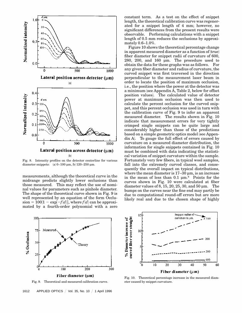
unobstructed beam intensity and phase at the celland detector planes, respectively. The location ofthe first minimum at ,236 µm at the cell and at,549 µm at the detector makes the actual profilesslightly wider than the equivalent Airy 53J11z2@z426pattern,6 which has its first minimum at 224 µm inthe cell and at 527 µm at the detector. This isexpected because the diffraction pattern at these twoplanes is not yet fully developed and will conse-quently be larger than the equivalent Airy pattern,which scales back to zero size at the pinhole.Figures 81a2 and 81b2 show profiles of intensity on
the detector centerline for essentially straight snip-pets 1s 5 1 m2 with various fiber diameters up to 250µm. The general shape of these curves is verysimilar to those generated with a one-dimensionalmodel.5 The first bright fringe in the 100-µm curveshown in Fig. 81a2 is slightly higher in magnitude
than the central bright fringe. This is unlike theone-dimensional predictions,5 in which the centraland the first bright fringes were found to be approxi-mately equal in size. Other differences appear inthe secondary fringe structure out between 500 and1000 µm, with the present results, in this region,more closely matching the measured profiles forlarge diameter fibers 1cf. Ref. 52. Notice that, unlikeFraunhofer diffraction, there is very little fringemovement with changing fiber diameter. As a checkon the validity of the computer code, the presenttwo-dimensional model was reduced to the one-dimensional equivalent used in Ref. 5 when E1j, h2 inEq. 142 was replaced with an Airy function and whenthe integration was ignored with respect to the hdirection. When this was done, identical resultswere obtained.The graph of Fig. 9 shows the theoretical calibra-
tion curve for the EBL with straight 2-mm-longsnippets compared with measurements on wirestaken from seven different Laserscan instruments.The experimental data were gathered by measure-ment of the occlusions at the detector, by the use of aTektronix 2465 digital readout oscilloscope and alsoby the use of software written for the purpose, and bymeasurement of wire diameters with the aid of aprojection microscope. The general shape of thetheoretical curve is in very good agreement with the
1a2
(b)
Fig. 7. Intensity and phase of the unobstructed beam at 1a2 thecell and 1b2 the detector from Fresnel diffraction of the Gaussianbeam at the pinhole.
measurements, although the theoretical curve in themidrange predicts slightly lower occlusions thanthose measured. This may reflect the use of nomi-nal values for parameters such as pinhole diameter.The shape of the theoretical curve shown in Fig. 9 iswell represented by an equation of the form Occlu-sion 5 10051 2 exp32f 1d246, where f 1d2 can be approxi-mated by a fourth-order polynomial with a zero
1a2
1b2
Fig. 8. Intensity profiles on the detector centerline for variousdiameter snippets: 1a2 0–100 µm, 1b2 120–250 µm.
Fig. 9. Theoretical and measured calibration curve.
constant term. As a test on the effect of snippetlength, the theoretical calibration curve was regener-ated for a snippet length of 4 mm; however, nosignificant differences from the present results wereobservable. Performing calculations with a snippetlength of 0.5 mm reduces the occlusions by approxi-mately 0.6–1.0%.Figure 10 shows the theoretical percentage change
in apparentmeasured diameter as a function of 1true2fiber diameter for snippet radii of curvature of 600,280, 200, and 160 µm. The procedure used toobtain the data for these graphs was as follows. Forany given fiber diameter and radius of curvature, thecurved snippet was first traversed in the directionperpendicular to the measurement laser beam inorder to locate the position of maximum occlusion,i.e., the position where the power at the detector wasa minimum 1see Appendix A, Table 2, below for offsetposition values2. The calculated value of detectorpower at maximum occlusion was then used tocalculate the percent occlusion for the curved snip-pet, and this percent occlusion was used in turn withthe calibration curve of Fig. 9 to infer an apparentmeasured diameter. The results shown in Fig. 10indicate that measurement errors for very tightlycrimped single snippets can be quite large andconsiderably higher than those of the predictionsbased on a simple geometric optics model 1see Appen-dix A2. To gauge the full effect of errors caused bycurvature on a measured diameter distribution, theinformation for single snippets contained in Fig. 10must be combined with data indicating the statisti-cal variation of snippet curvature within the sample.Fortunately very few fibers, in typical wool samples,fall into the extremely curved classes, and conse-quently the overall impact on typical distributions,where themean diameter is 17–30 µm, is an increasein the mean of less than 0.1 µm.8 Points for thecurves shown in Fig. 10 were calculated at fiberdiameter values of 8, 15, 20, 25, 30, and 50 µm. Thebumps on the curves near the fine end may partly bedue to computational round-off errors but are morelikely real and due to the chosen shape of highly
Fig. 10. Theoretical percentage increase in the measured diam-eter caused by snippet curvature.
curved snippets. Because of practical difficulties anaccurate experimental verification of the findingsshown in Fig. 10 has proved extremely difficult, butmeasurementsmade on straight and curved 1s , 200µm2 44-µm wires indicate that the results are of thecorrect magnitude.Figures 111a2–111c2 show computer-generated plots
of normalized intensity at the detector for a 50-µmsnippet with a radius of curvature of 1a2 1 m, 1b2 600µm, 1c2 280 µm, 1d2 200 µm, and 1e2 160 µm. Thebright circle near the periphery of these figuresindicates the edge of themeasurement photodetector.The apparent step nature of this circle, which is alsovisible as artifacts within the intensity plots, arisesfrom each image that is originally 128 3 128 pixelsin size being expanded to 512 3 512 pixels, whichoccurs through a simple scheme of setting each fouradjacent pixels to the same intensity. The fringestructure in the diffraction patterns is clearly vis-ible, as is the distortion of its symmetry with smallerradii of curvature. Although for larger radii ofcurvature the light from one of the bright secondaryfringes initially appears to be displaced into its
1a2 1b2
1c2 1d2
1e2
Fig. 11. Theoretically generated diffraction patterns at the mea-surement detector in the Laserscan resulting from a 50-µmdiameter snippet that is 1a2 straight or has a radius of curvature of1b2 600 µm, 1c2 280 µm, 1d2 200 µm, or 1e2 160 µm. The white circlesshow the location of the edge of themeasurement detector, and thesnippet ends curve progressively more to the left of each figure.
opposite partner, at the smaller radii of curvature adeep dark patch develops and results in a rapid lossof power at the detector.
5. Conclusions
The effect caused by snippet curvature on measure-ment in the pinhole-apertured expanding beam La-serscan has been modeled by the use of two-dimensional Fresnel diffraction. The magnitude ofthe effect for single curved snippets is considerablylarger than that of the predictions based on a simplegeometric shadowing model. The increase in beamocclusion at the detector can be explained by thedevelopment of a dark patch in the diffraction pat-tern at very small snippet radii of curvature. Anumber of simplifying techniques enable one tospeed up computations arising from the complextwo-dimensional Fresnel diffraction formulation by2–3 orders of magnitude, thereby permitting investi-gations to be performed on a personal computer.
Appendix A. Geometric Optics Estimation of Errors
The geometric optics model outlined here estimatesthe errors when curved snippets are measured in theLaserscan by considering the optics in terms of avery simple geometric shadowing model. The sizeof the measurement beam at the cell is first trans-formed to an equivalent top-hat or uniform intensityprofile beam, which would result in the correctmeasured beam occlusions at the detector. Simplegeometry is then used to find the longer length ofcurved fiber, in contrast to straight fiber, whichmasks light from the beam, and this subsequentlyallowsmeasurement differences between curved andstraight fibers to be expressed in terms of an errorratio.For a circular measurement beam of uniform
intensity I0 and radius R , the total power withinthe beam is I0pR 2. If a straight fiber of diameter dis placed in the beam so as to divide it symmetrically,then, ignoring any end effects, we see that the powermasked from the beam by the fiber is 2I0R d.Consequently the occlusion, O`, or fraction of powerlost from the beam is simply
O` 5 12I0R d2@1I0pR22
5 12d2@1pR2, 1A12
so that for any given beam occlusion associated witha given fiber diameter, the equivalent top-hat beamradius is
R 5 12d2@1pO`2. 1A22
Table 1 shows the equivalent top-hat beam radius forthree fiber diameters calculated from relation 1A22,with the values forO` coming directly from a polyno-mial fit to occlusionmeasurements made in the EBL.The geometry for determining the length of curved
snippet occluding a fictitious top-hat profile beam isshown in Fig. 12. The arc length c of the curvedfiber centerline, whose radius of curvature is s, is
so that again ignoring end effects, we see thatocclusionOs for a curved fiber is found from
Os 5 12I0sbd2@1I0pR22
5 12sbd2@1pR22. 1A42
Consequently the error ratio, e, of occlusion for thestraight fiber to occlusion for the curved fiber is
e 5 1sb2@R. 1A52
We can obtain angle b by noting that arc length c,and hence the occlusion, will be a maximum whenpoints of intersection T and U lie on the diameter ofthe circle defined by the top-hat beam periphery.From simple geometry we then have
b 5 sin211R@s2. 1A62
By also noting that
cos b 5 1s 2 joff2@s 1A72
and substituting for cos b in terms of sin b, we findthat the offset of the curved fiber centerline, atmaximum occlusion, is given by
joff 5 s 2 1s2 2 R 221@2. 1A82
By using the values of R shown in Table 1 andEqs. 1A52 and 1A62, we can calculate the occlusionerror ratio for a given fiber diameter and radius of
Table 1. Top-Hat Beam Radius for Given Fiber Diameters
curvature. This can then be used to calculate theapparent measured occlusion for the curved fiber,which in turn can be used to infer an apparentmeasured diameter from the polynomial fit to occlu-sion measurements made in the EBL. The result ofthese calculations is shown in Table 2 as the percent-age increase in apparent measured diameter, alongwith the 1geometric optics2 fiber offset at maximumocclusion from Eq. 1A82 compared with the offsetfound from the two-dimensional Fresnel diffractionmodel.The results summarized in Table 2, when com-
pared with the Fresnel diffraction results of Fig. 10,show that the geometric optics model generally givesa considerable underestimate of the apparent errorswhen measuring curved fibers. Note that the offsetfor maximum occlusion, in the Fresnel diffractionmodel, was found to be approximately constant foreach fiber radius of curvature. This is not the casein the geometric optics model.
Appendix B. Nomenclature
a, distance from pinhole to measurementcell plane,
a0, laser beam wave-front radius of curva-ture at the pinhole,
b, distance from measurement cell planeto detector plane,
A, aperture formed by transparent regionat the measurement cell plane,
c, curved fiber arc length in geometricoptics model,
d, diameter of snippet or width of opaquestrip mask,
D, pinhole diameter,dS, element of area djdh at the measure-
ment cell plane,E1j, h2, vector illumination field at themeasure-
ment cell plane,i, Œ21,
I1x8, y82, intensity at point P:1x8, y82 on the detec-tor,
I0, intensity of top-hat profile beam in geo-metrical optics model,
J0, zero-order Bessel function of the firstkind,
J1, first-order Bessel function of the firstkind,
k, wave number 2p@l,n, refractive index,O, origin of coordinate system x–y–z at the
measurement cell plane,O8, origin of coordinate system x8–y8–z8 at
the center of the pinhole,O`, occlusion of straight fiber in geometric
optics model,P, observation point on the detector,
Q, general point with coordinates 1j, h2 atthe measurement cell plane,
Q8, general point with coordinates 1j8, h82 atthe pinhole plane,
r, radial coordinate at the detector plane,R, radius of measurement detector,R , radius of top-hat profile beam in geomet-
ric optics model,s, distanceQP,s8, distanceQ8P,t, thickness of medium of refractive index
n,T,U, intersection points of curved fiber center-
line and periphery of top-hat profilebeam in geometric optics model,
x–y–z, coordinate system centered at O at themeasurement cell plane,
x8–y8–z8, coordinate system centered at O8 at thecenter of the pinhole,
x8, y8, z8, coordinates of point Pwith respect toO8,z8, a 1 b,z08, laser beam waist to pinhole spacing,zR, Rayleigh range of laser beam waist,
pv02@l,
a, angle subtended by the curved snippetin the Fresnel model,
b, half-angle subtended by the illuminatedcurved fiber in the geometric opticsmodel,
e, occlusion error ratio in the geometricoptics model,
hi,max8, distance from x8 axis to outermost pointon inner circular arc,
ho,max8, distance from x8 axis to outermost pointon outer circular arc,
u, angular coordinate at the pinhole plane,U, angle between lineO8P and z8 axis,l, wavelength,
joff, offset off snippet centerline from y8 axis,
ji8, x8 coordinate on inner circular arc forgiven h8,
jo8, x8 coordinate on outer circular arc forgiven h8,
j, h, coordinates of a general point Q withrespect to O at the measurement cellplane,
j8, h8, coordinates of a general point Q8 withrespect toO8 at the pinhole plane,
r, radial coordinate at the pinhole plane,s, radius of curvature of snippet or mask
centerline,si, radius of curvature of snippet inner
circular arc,so, radius of curvature of snippet outer
circular arc,f, angular coordinate at the detector plane,
c1P2, vector field at point P on the detector,c01P2, unobstructed vector field at point P on
the detector,cm1P2, vector field at point P on the detector
caused by a transparent strip mask atthe cell plane,
v, 1@e amplitude radius of the laser beam,v0, 1@e amplitude radius of the laser beam
at the beam waist.
Support for this project was provided by Austra-lian Woolgrowers and the Australian Governmentthrough the International Wool Secretariat and theCommonwealth Scientific and Industrial ResearchOrganization.
References1. L. J. Lynch and N. A. Michie, ‘‘Laser fineness distribution
analyser: a device for the rapid measurement of the meanand distribution of the fibre diameter,’’ Wool Technol. SheepBreed. 20, 22–27 119732.
2. L. J. Lynch and N. A. Michie, ‘‘An instrument for the rapid
automatic measurement of fiber fineness distribution,’’ Text.Res. J. 46, 653–660 119762.
3. M. Kerker, The Scattering of Light and Other ElectromagneticRadiation, 1st ed. 1Academic, New York, 19692, Chap. 4, p. 179.
4. M. Glass, ‘‘A mathematical model of the wool fiber diameteranalyser 1FDA2,’’ Lab. Note SN@125 1Commonwealth Scientificand Industrial Research Organization, Division of Wool Tech-nology, Sydney, Australia, 19912.
5. M. Glass, T. P. Dabbs, and P. W. Chudleigh, ‘‘The optics of thewool fiber diameter analyser,’’ Text. Res. J. 65, 85–94 119952.
6. M. Born and E. Wolf, Principles of Optics, 6th ed. 1Pergamon,NewYork, 19802, Chap. 8, p. 382.
7. H. Kogelnik, ‘‘On the propagation of Gaussian beams of lightthrough lenslike media including those with a loss or gainvariation,’’Appl. Opt. 4, 1562–1569 119652.
8. T. P. Dabbs, H. van Schie, and M. Glass, ‘‘The effect of fibercurvature on Laserscan diameter measurement,’’ presented atthe International Wool Textile Organisation Committee Meet-ing, Nice, France, 4–9 December 1994.
9. F. A. Jenkins and H. E. White, Fundamentals of Optics, 3rd ed.1McGraw-Hill, Tokyo, 19572, Chap. 2, p. 20.