Bachelor Thesis Friendly Interchange Heuristic for Vehicle Routing Problems with Time Windows Author: SSJ Jaheruddin Supervisor: M.J.P. Peeters 575600 A Thesis submitted in partial fulfillment of the requirements for the degree of Bachelor in Econometrics and Operations Research Faculty of Economics and Business Administration Tilburg University August 16, 2010
Transcript
Bachelor Thesis
Friendly Interchange Heuristic for Vehicle Routing Problems
A Thesis submitted in partial fulfillment of the requirements for the degree of Bachelor in Econometrics and Operations Research
Faculty of Economics and Business Administration Tilburg University
August 16, 2010
1
1. Abstract Vehicle Routing Problems with Time Windows (VRPTW) are hard to solve, and even small instances resist ways to find the optimal solution. Therefore heuristics are used to get good solutions. In this paper heuristics that are currently used to find the best known solutions are briefly described. Also the entirely new Friendly Interchange Heuristic (FIH) is introduced and its results are compared to the best known solutions for benchmark problems.
4. Tour Creation ...................................................................................................................................... 4
4.2.2 Multiple Ant Colony System ...................................................................................................... 5
5. Local Search ........................................................................................................................................ 6
5.1 General Pair wise Interchange Neighborhood .................................................................................. 6
5.2 General k-way Interchange Neighborhood ...................................................................................... 7
A4 Computation times .......................................................................................................................... 27
3
3. Introduction A Vehicle Routing Problem with Time Windows (VRPTW) is a problem where several cities have deterministic demand. Each city has to be visited exactly once, and within a specific time interval. There is one depot from which trucks with a certain loading capacity depart simultaneously. There are several possible objective functions that minimize combinations of the amount of trucks, the amount of kilometers, or even the amount of time required. In this paper the main goal is to minimize the number of vehicles, and as a tie breaker the number of kilometers is minimized. To test heuristics for VRPTW a set of benchmark problems has been created, the so called Solomon instances (Solomon 2005). Each problem consists of exactly 100 cities that can be either randomly distributed, clustered or both. Also the time constraints for the problem can be loose, or tight. The distances are Euclid, and one kilometer takes one unit of time. VRP is NP hard, as VRPTW can be reduced to VRP with some restrictions VRPTW is also NP hard (Solomon 1987). Considering this, solving for optimality is not an option for problems of some size, and therefore heuristics must be designed to find good solutions. In this paper we will construct a heuristic for VRPTW by using several elements from existing heuristics as a basis. After implementing and combining these, a new neighborhood will be added. The latter is called the Friendly Interchange Neighborhood, an extension of the general k-way Interchange Neighborhood that we shall describe in this paper.
4
4. Tour Creation When creating tours one can choose between a sequential and a parallel method (Solomon 1987). With a sequential method, in each step one truck is selected and customers are added to the route of that truck. When required a new truck is added, this goes on until all customers are served. With a parallel method a number of truck routes are being altered within one step. This means that there is some freedom in the number of trucks that is used in the beginning. Both the sequential and the parallel method can be applied deterministically, or generically. The main idea behind generic algorithms is that the sum of all best sub decisions, does not generally add up to the best total combination of decisions. But of course, the probability that a good sub decision is part of the best total solution is relatively high. Therefore generic algorithms often give sub decisions that seem favorable a higher probability. Now the decisions just need to be made many times, and hopefully one of all the solutions that are found is good. After all, when solving a problem the average solution that you find is not interesting, only the best one is.
4.1 Examples sequential method
4.1.1 Nearest Neighbor
There are many deterministic sequential tour creation algorithms like Nearest Neighbor and Insertion. To give simple deterministic example of a sequential tour creation we define the Nearest Neighbor algorithm NN1 as follows: 1) Start driving with 1 truck. 2) Add the available city with the lowest penalty cost Cij. 3) Repeat this until no city can be added. 4) Start driving with the next truck. 5) If not all customers are served go to 2). This is the Nearest Neighbor algorithm for which Solomon proposed a cost function. However, when the right parameters are set it is generally outperformed by Insertion (Solomon 1987). The mentioned cost function is defined as follows: Cij= δ1Dij+ δ2Tij+ δ3Vij s.t. δ1+ δ2+ δ3=1, δ1≥0, δ2≥0, δ3≥0
i is in the partial solution, j is not in the partial solution. with: Dij:= Euclid distance from i to j. Tij:= Time difference between completing i and starting j. Vij:= Time remaining until last possible start of j following i.
4.1.2 Probable Nearest Neighbor
Though generic sequential algorithms are not often used in practice, we can easily create an example by adapting step two of the Nearest Neighbor algorithm. Assuming positive costs, the second step could become: 2) Add an available city with probability SC/Cij. Where SC is defined as the sum of costs over all available cities j from current point i.
5
4.2 Examples parallel method
4.2.1 Savings Heuristic
An example of a deterministic parallel method is given by Solomon (1987):
1) Begin with n trucks that each serve 1 customer each.
2) Try to connect all end points of a truck to the starting point of all new trucks and calculate
costs.
3) Pick the single satisfactory connection with the lowest total Euclid distance.
4) If another satisfactory connection can be made go to 2).
Where a satisfactory connection is defined as feasible and with an increase in waiting time
lower than a constant upper bound. This upper bound should be set in advance.
4.2.2 Multiple Ant Colony System
To conclude this section we give a more interesting example of how important tour creation can be in a heuristic. Perhaps the best generic building method that exists today is the Multiple Ant Colony System (Gambardella 2000). This heuristic was based on the behavior of food searching ants in nature, and has one ant colony per objective. First of all a number of ants finds a feasible solution to the VRPTW problem by randomly choosing a feasible city to visit each time, while using a uniform distribution to choose between possible cities. When an ant visits the depot to drop its load, it counts as adding a truck. After the ants have completed their task their pheromone trace is left behind to attract ants from the next wave to the edges visited by the past ant wave. Every colony leaves a specific trace behind that is only picked up by other ants in the same colony. The strength of the pheromone trace of a single ant is correlated with the quality of the solution. For example, an ant that comes from a colony that has as objective to minimize the number of kilometers, will leave a trail with strength one over the number of kilometers it travelled before finding a feasible solution. After this first run, a second wave of ants sets out to search food. Again they randomly choose cities each time, but they do not use a uniform random distribution, but one that is affected by the pheromones. A stronger pheromone trail is more likely to attract an ant. Therefore they are more likely to take good routes than they would have been without the existing pheromone traces. Note that the ant leaves the same trace behind on all roads between cities it visited, so if an ant goes from the depot to A to B to C to D and another ant goes from the depot directly to C, then it can still pick up the pheromone trail which tells it that the other ant went to D afterwards, with good or bad result. Several groups of ants go out on a hunt for food after another and each group has better information than the previous one, resulting in better solutions. Initially the algorithm was designed in such a way that ants were attracted by the pheromones of all predecessors. However, the most recent version only uses information from the best solution to influence ants.
6
5. Local Search
A local search algorithm finds better solutions by browsing the neighborhood of an existing solution. It is customary to go by all neighbors 1 by 1 until a certain target is reached. This target can be the improvement of the current solution or finding the best neighbor. When using the first improvement the steps are faster as not all neighbors need to be checked. When using the best solution instead the number of required steps is generally lower and the result does not depend on the order in which you compare the neighbors. A more sophisticated target would be dependent on your objective function. For example, pick the first neighbor that requires less trucks, and otherwise the one with the least amount of kilometers. This is the criterion that is used in this paper. In this chapter several neighborhoods will be described, most of which form the foundation of the Friendly Interchange Heuristic.
5.1 General Pair wise Interchange Neighborhood
This is perhaps the most simple neighborhood. It selects two cities in the solution, not necessarily from one truck tour, and switches their places like shown in figure 1.
Figure 1: Pair wise Interchange move
This neighborhood is frequently used in job shop problems (Morton, T. E. & Pentico, D.W., 1993) but not in VRP heuristics as it cannot reduce the number of vehicles and cannot change sections of a tour. However, this algorithm is rather quick, and might be useful to improve the starting point.
7
5.2 General k-way Interchange Neighborhood
An extension of the GPIN is the Gk-IN as described by Morton, T. E. & Pentico, D.W. (1993). Now not only pairs are selected, but every combination of k points, not necessarily from 1 tour. And after selecting these k points try all possible ways of swapping and look for the best improvement. As searching the entire neighborhood is of O(Nk) this neighborhood is not frequently used for k>3. Despite the fact that this algorithm is very costly for large k, the required computational time can be managed by using it on problems with a small N. This could mean that it is used for VRPTW instances with not many cities, or that it is used for parts of an instance. For example it can be used to improve the efficiency of 1 truck. Or even to consider many interchanges of cities that are visited within a limited time interval. This can be particularly effective for instances with tight time constraints.
Another way to search the Gk-IN is by means of a trick we have invented to significantly reduce the number of solutions in the neighborhood. When observing a Gk-IN we noticed that many of the solutions are in fact in the G(k-1)-IN. For example the permutations of 1 2 3 and 4 can be divided in a group that is in the 3 Interchange Neighborhood, and a group that is not in the 3 Interchange Neighborhood. Note that solutions are not symmetric due to time windows, 3214 is not the same as 4123 as it might be possible to add a fifth city to 3214 while it may not be possible to add the same city to 4123. Here is an example of what the 4-way Interchange Neighborhood of a small tour looks like and how it is split up:
In 3-way Interchange Neighborhood Not in 3-way Interchange Neighborhood
1234 2143
1243 2341
1324 2413
1342 3142
1423 3412
1432 3421
2134 4123
2314 4312
2431 4321
3124
3214
3241
4132
4213
4231 Table 1: 4-way Interchange Neighborhood
This can be exploited by first performing 3-way Interchange, and after that only searching the solutions that are not in the 3-way Interchange Neighborhood. Of course after improving it in this way the other moves need to be checked again to make sure that it is not possible to improve further with 3-way Interchange moves, but as most solutions that are checked do not lead to improvements this can save much time. When no improvement is found this method takes less than half the time that normal k-way Interchange would take. In the worst case this way of doing k-way Interchange has the same complexity as normal k-way Interchange, the only drawback is that you can no longer compare all k-Interchange improvements if you First make a solution by executing all (k-1)-way Interchanges that lead to improvement, which probably leads to a loss in quality of the end result. Therefore this way of browsing the k-IN, Opt or Opt* Neighborhood has not been implemented in the final version of the Friendly Interchange Heuristic.
8
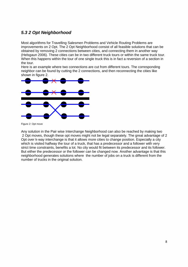
5.3 2 Opt Neighborhood
Most algorithms for Travelling Salesmen Problems and Vehicle Routing Problems are improvements on 2 Opt. The 2 Opt Neighborhood consist of all feasible solutions that can be obtained by removing 2 connections between cities, and connecting them in another way (Helsgaun 2006). These cities can be in two different truck tours or within the same truck tour. When this happens within the tour of one single truck this is in fact a reversion of a section in the tour. Here is an example where two connections are cut from different tours. The corresponding neighbor can be found by cutting the 2 connections, and then reconnecting the cities like shown in figure 2.
Figure 2: Opt move
Any solution in the Pair wise Interchange Neighborhood can also be reached by making two 2 Opt moves, though these opt moves might not be legal separately. The great advantage of 2 Opt over k-way interchange is that it allows more cities to change position. Especially a city which is visited halfway the tour of a truck, that has a predecessor and a follower with very strict time constraints, benefits a lot. No city would fit between its predecessor and its follower. But either the predecessor or the follower can be changed now. Another advantage is that this neighborhood generates solutions where the number of jobs on a truck is different from the number of trucks in the original solution.
9
5.4 k Opt Neighborhood
In general k Opt moves can be made by removing k connections and connecting them in all feasible ways (Helsgaun 2006). However, due to the strongly increasing computation time 2 Opt and 3 Opt are most popular, and k>5 is rarely used. This neighborhood seems to give very good results for VRP problems. Especially when combined with an algorithm that selects how large k is at each step, this is called the Lin-Kernighan heuristic.
5.4.1 Lin Kernighan Helsgaun
One of the best heuristics that uses local search was described in a paper by Lin, S.& Kernighan, B.W. (1973). It is called the Lin Kernighan heuristic and searches the k Opt Neighborhood for various k. The most popular implementation is Helsgaun’s. A Lin Kernighan heuristic with Helsgaun’s (2006) implementation is abbreviated to LKH. The LKH is used in the following way: First do a lot of trials and find many random feasible solutions. Note that LKH is not called a generic heuristic because creation of initial solutions is not considered to be part of the actual improvement algorithm. Then merge parts of good solutions by fixing edges that occur in many good solutions to get even better solutions. After this let a function determines which k Opt Neighborhood to search. For calculation purposes the Lin Kernighan Helsgaun implementation first tries to shift several sequential cities within a single truck route and check if the result is an improvement. The length of these segments of truck routes is at most k. When no more improvements are found a possible next step is again to fix the edges that appear in many good tours and then optimize the rest with larger k.
10
5.5 2 Opt* Neighborhood
This is a neighborhood that specifically has been designed for VRPTW problems (Thangiah, S.R., Sun, T. & Potvin, J., 1996). The neighborhood is a restricted version of the 2 Opt Neighborhood. Only Tails from two different tours are cut. As a result, when swapping tour sections, the order of cities within a tour section will not change.
5.6 k Opt* Neighborhood
As Thangiah, S.R., Sun, T. & Potvin, J. (1996) only defined 2 Opt*, we will define k Opt* here as k Opt with the restriction that the tails of k different truck tours are cut. This ensures that the order of cities within a tour section will not change.
5.6.1 LKH for VRPTW
An adaptation of the normal LKH has been made by Holden, N. & Hasle, G. (2009). Unfortunately the results did not turn out to be great. This might be caused by the fact that the merging of tours by fixing edges that occur in multiple good solutions has completely been removed to keep it simple, but it could also mean that LKH is not suitable for VRPTW. However, from this implementation we took the concept of not always making the same large move. When deciding on which problems to investigate first many Quick moves were made as will be described later.
11
5.6 Cross Exchange Neighborhood
A neighborhood that is particularly effective for solving VRPTW problems is the Cross Exchange Neighborhood as stated by Bai, R. Burke, E.K., Grendeau, M. &Kendall, G. (2007). This neighborhood is found by picking all possible sections from two different truck tours, and interchanging them. This has as an advantage that the order of cities within the segment is unchanged, and therefore time windows within the section are unlikely to cause problems. Figure 3 is an example of two tour sections with one two and one cities respectively that are exchanged.
Figure 3: Cross Exchange move
Note that the Cross Exchange Neighborhood also contains solutions which require fewer trucks then the initial solution. Cross exchange can move cities from a first truck to a second truck without moving any cities from the second truck to the first. And thus a truck can end up visiting zero cities and then the number of trucks will be decreased.
5.7 k Cross Exchange Neighborhood
The Cross Exchange Neighborhood has only been defined as interchanging two sections from two different tours. However, k Cross Exchange has not been defined yet. In this paper we define the k Cross Exchange Neighborhood as a generalization of the Cross Exchange Neighborhood. In the k Cross Exchange Neighborhood not only segments from two tours are exchanged. But all possible sections from k different truck tours are exchanged, while again the order of cities within a section remains the same. Like with Cross Exchange the length of these sections can be anything from zero to the size of the truck tour.
12
6. Friendly Interchange Heuristic In this paper we propose a new heuristic for Vehicle Routing Problems with Time Windows. The so called Friendly Interchange Heuristic (FIH) first creates a starting solution and then tries to improve it until a good solution is found. For creating an initial solution we created a cost function for the Nearest Neighbor heuristic that uses only two parameters and performs quite well compared to other tour creation heuristics. After this initial solution has been created, a Quick method is used to improve the initial solution to a decent solution. This Quick method searches a small part of the entire neighborhood that is searched for tour improvement. Though this is not a necessary in between step in the algorithm as it is possible to use all improvement methods on the initial solution. This Quick method is used to improve the starting solution with many quick steps in order to reduce calculation time. Once the Quick method can no longer find any improvements, the algorithm enters the final tour improvement stage. Here a large neighborhood is searched to look for improvements, this is a time consuming process but due to the Quick method only a few steps are required to reach the best possible solution.
6.1 Initial solution
It has been recommended to use Insertion for VRPTW problems as it outperforms Nearest Neighbor (Solomon 1987). The suggested insertion criterion I1 uses two insertion criteria: ‘Farthest unrouted customer’ or ‘Unrouted customer with earliest deadline’. This indeed outperforms the Nearest Neighbor algorithm NN1 when it uses a linear cost function that is both dependant on time and Euclid distance as described in Tour Creation: Cij= δ1Dij+ δ2Tij+ δ3Vij s.t. δ1+ δ2+ δ3=1, δ1≥0, δ2≥0, δ3≥0 i is in the partial solution, j is not in the partial solution. with: Dij:= Euclid distance from i to j. Tij:= Time difference between completing i and starting j. Vij:= Time remaining until last possible start of j following i. However, in this paper we provide a completely new Nearest Neighbor implementation, called NN2, a sequential algorithm that can compete with the suggested Insertion algorithm, and that outperforms Nearest Neighbor on almost every problem set while using one parameter less: Cij= δ1Dij Dij + δ2Tij Tij s.t. δ1+ δ2=1, δ1≥0, δ2≥0 i is in the partial solution, j is not in the partial solution. with: Dij:= Euclid distance from i to j. Tij:= Time difference between completing i and starting j.
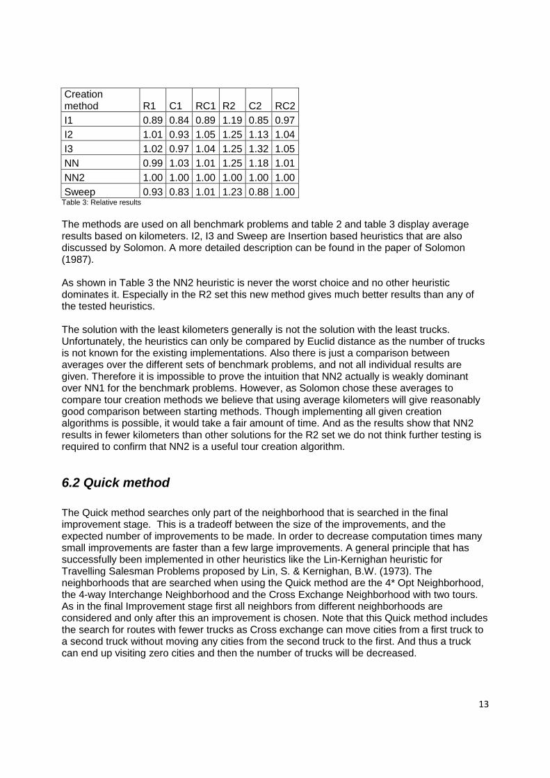
The methods are used on all benchmark problems and table 2 and table 3 display average results based on kilometers. I2, I3 and Sweep are Insertion based heuristics that are also discussed by Solomon. A more detailed description can be found in the paper of Solomon (1987). As shown in Table 3 the NN2 heuristic is never the worst choice and no other heuristic dominates it. Especially in the R2 set this new method gives much better results than any of the tested heuristics. The solution with the least kilometers generally is not the solution with the least trucks. Unfortunately, the heuristics can only be compared by Euclid distance as the number of trucks is not known for the existing implementations. Also there is just a comparison between averages over the different sets of benchmark problems, and not all individual results are given. Therefore it is impossible to prove the intuition that NN2 actually is weakly dominant over NN1 for the benchmark problems. However, as Solomon chose these averages to compare tour creation methods we believe that using average kilometers will give reasonably good comparison between starting methods. Though implementing all given creation algorithms is possible, it would take a fair amount of time. And as the results show that NN2 results in fewer kilometers than other solutions for the R2 set we do not think further testing is required to confirm that NN2 is a useful tour creation algorithm.
6.2 Quick method
The Quick method searches only part of the neighborhood that is searched in the final improvement stage. This is a tradeoff between the size of the improvements, and the expected number of improvements to be made. In order to decrease computation times many small improvements are faster than a few large improvements. A general principle that has successfully been implemented in other heuristics like the Lin-Kernighan heuristic for Travelling Salesman Problems proposed by Lin, S. & Kernighan, B.W. (1973). The neighborhoods that are searched when using the Quick method are the 4* Opt Neighborhood, the 4-way Interchange Neighborhood and the Cross Exchange Neighborhood with two tours. As in the final Improvement stage first all neighbors from different neighborhoods are considered and only after this an improvement is chosen. Note that this Quick method includes the search for routes with fewer trucks as Cross exchange can move cities from a first truck to a second truck without moving any cities from the second truck to the first. And thus a truck can end up visiting zero cities and then the number of trucks will be decreased.
14
6.3 Improvement Algorithm
The final stage of the Friendly Interchange Heuristic (FIH) consists of an improvement algorithm that searches a large neighborhood. It mainly focuses on decreasing the number of total kilometers as most of the minimization regarding the number of trucks has already taken place in creating the initial solution and by applying the Quick Method. However in each step it quickly checks if the number of trucks can be reduced. After several neighborhoods are searched, the best neighbor of all these neighborhoods combined is chosen and this will be seen as the new starting point. Three conventional methods have been combined to give this final improvement stage of the FIH a firm foundation. Note that these can partially be skipped when searching for the first improvement when the Quick method has been used to improve the initial solution. 1) As improvement by Opt* moves has provided good results (Holden, N. & Hasle, G., 2009) these Opt* moves are also used in FIH. As most best known solutions either use at most 5 or at least 10 trucks, 5 has been chosen as the largest Opt* Neighborhood that is searched. As only moves between tours are made 6 Opt* or higher does not add anything for solutions with at most 5 trucks. And as searching an Opt neighborhood becomes significantly more work when more trucks are used, anything over 5 Opt* is inapplicable to solutions with more than 10 trucks. For reference, checking the 5 Opt* neighborhood for a solution with 13 tours takes roughly 4.5 hours as shown in Appendix A4. 2) As it is a small step from Opt* to Interchange, the best 5-way Interchange move is also considered. Though Interchange itself is not as strong as Opt*, it is a useful combination as Interchange covers a major weakness in Opt*. Interchange has the ability to optimize the order of cities within a tour, a feature that Opt* lacks . 3) It is stated by Bai, R., Burke, E.K., Grendeau, M. & Kendall, G. (2007) that Cross Exchange is very effective for VRPTW problems. Cross Exchange was applied with segments from two tours, and we have improved on this by checking the Cross Exchange Neighborhood with segments from two or three tours. The Cross Exchange does not only allow for improvements in the number of kilometers, but also in the number of required trucks. Even though Cross Exchange with three tours is not mentioned in the description of any record holding VRPTW heuristic (Solomon 2005), implementing this does not yet lead to the best known results. Therefore we designed a completely new method to improve VRPTW solutions. Note that this new neighborhood is also completely searched like the neighborhoods corresponding with the three methods above, and only after this the best improvement from all these neighborhoods is selected and executed. For every city Ci a k-friend list is made based on time and location. The friend list is an entirely new concept we have developed and it will be described now. The ready time of the predecessor of Ci and the due date of the follower of Ci determine which cities are potential friends. For the calculations we have chosen to fill the friend list with Ci, the predecessor of Ci, the follower of Ci, and the k potential friends with the smallest Euclid distance from Ci. This could result in a friend list as displayed in figure 4.
15
Figure 4: Friend list
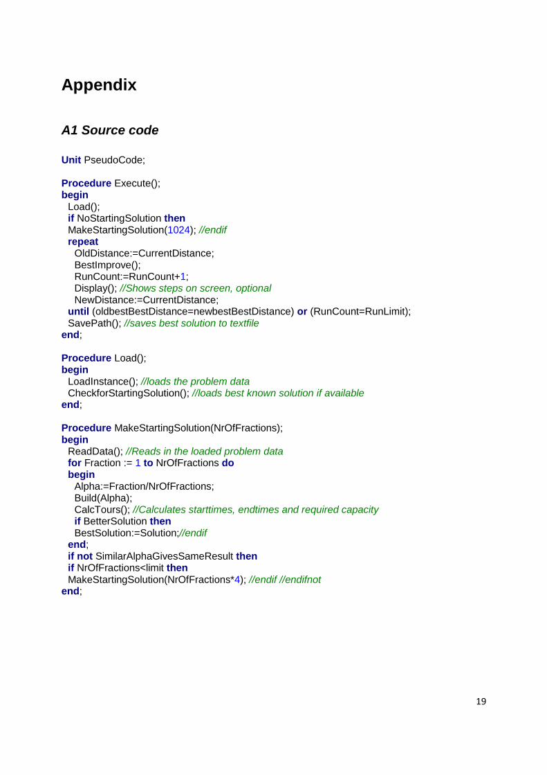
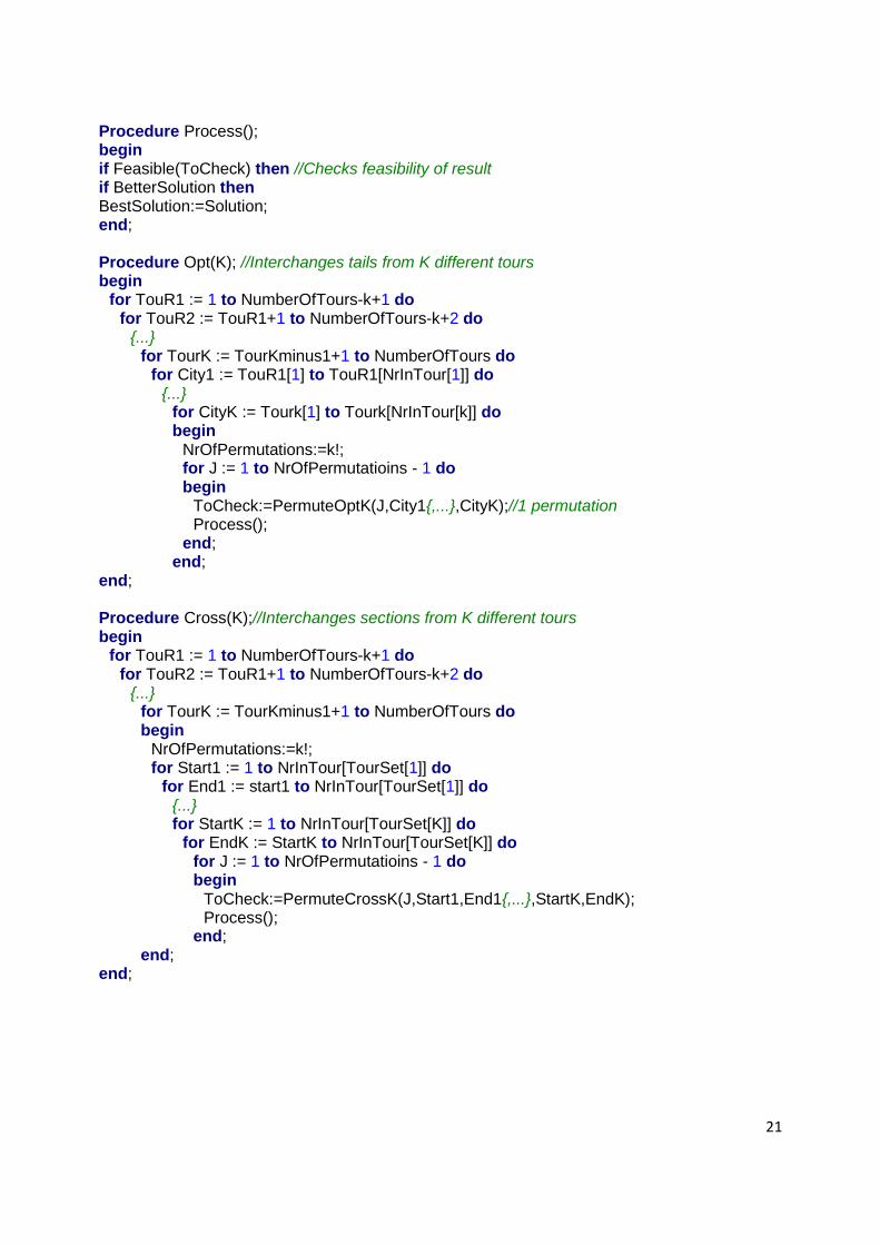
The large dot is city Ci, and together with the circled dots they make it makes up a friend list of size 10. This is the same size that has been used in the implementation as checking all interchange moves for the 100 cities roughly takes 20 minutes with 1GHZ available. Checking N friend lists of size 12 on the other hand, would take more than one day. After the friend list has been made all k! possible interchanges between these k points are considered for all N cities. As these points, given each city Ci with i 1 to N, are relatively close to each other in distance and time, it is likely that many interchanges are smart and feasible. This method is particularly interesting as it using it for all hundred cities in the benchmark problems is roughly as fast as normal 4-way Interchange, therefore it can make moves that would be incalculable when not only the friend list had to be considered. In addition to using this friend list for k-way Interchange, we have also implemented the check of all Opt* moves with these k starting points, even if they are not all in different tours. However, note that most Opt* moves will be infeasible unless a solution has many trucks that visit only a few cities. This was a brief description of the Friendly Interchange Heuristic, the entire program in pseudo code can be found in appendix A1.
16
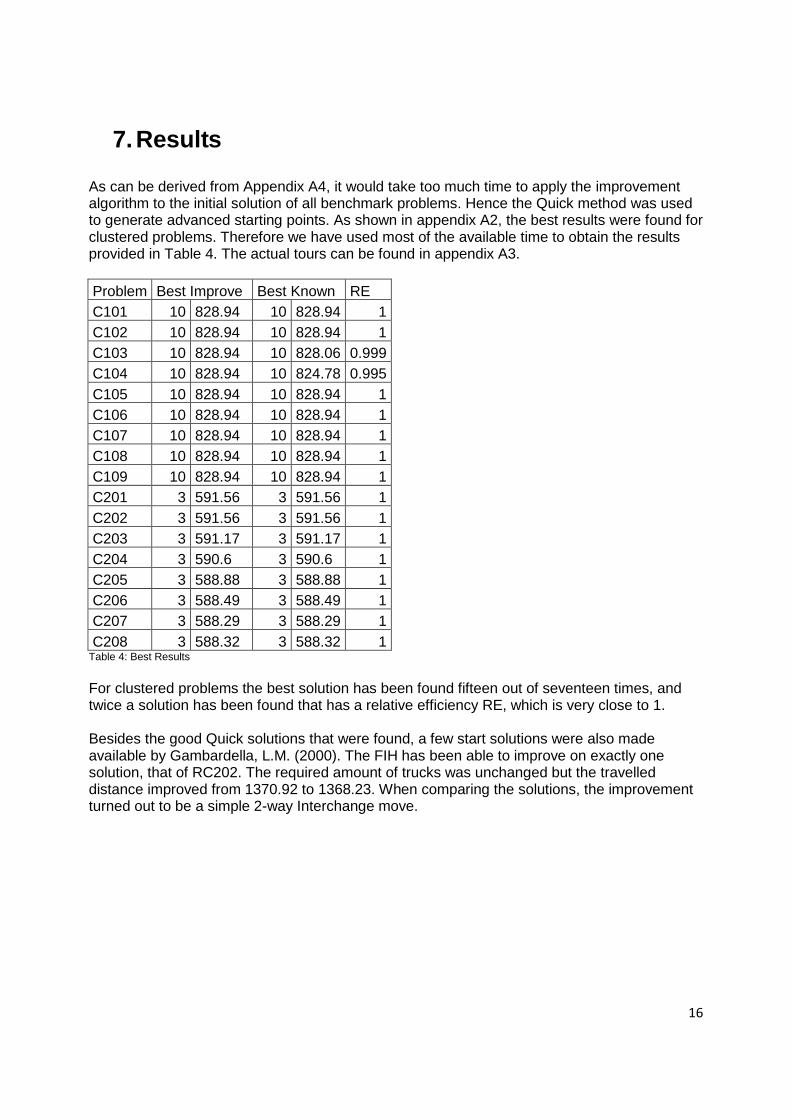
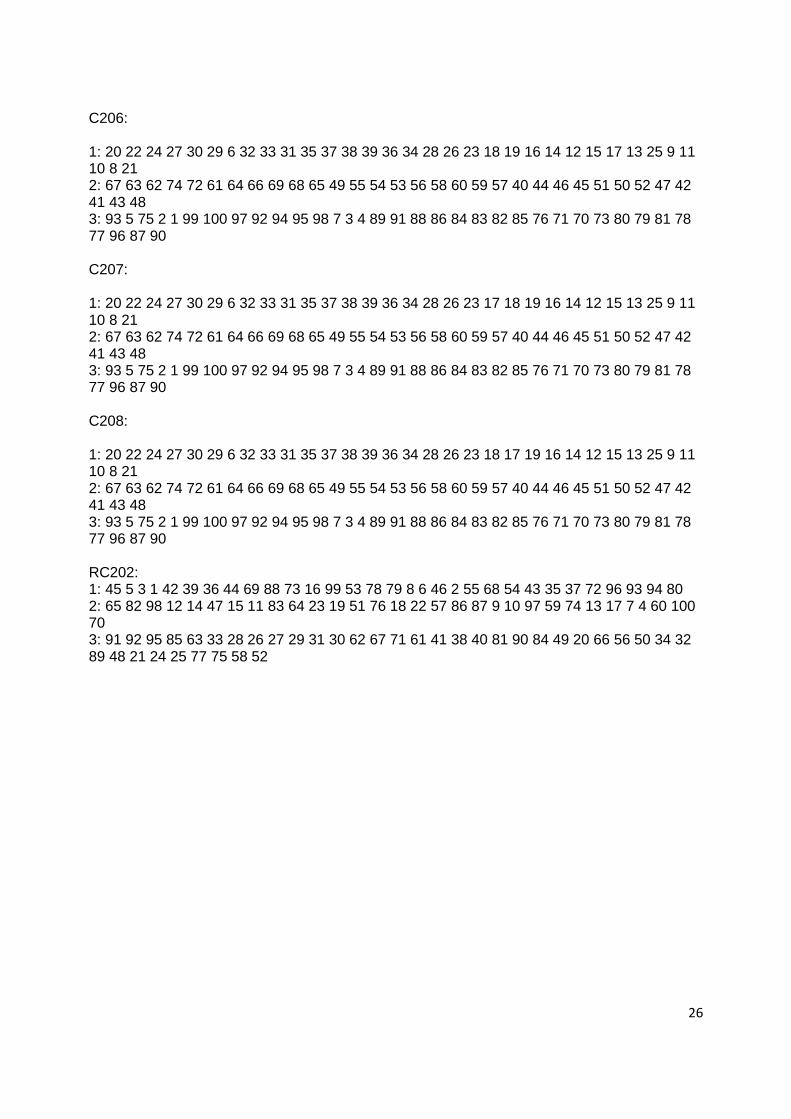
7. Results As can be derived from Appendix A4, it would take too much time to apply the improvement algorithm to the initial solution of all benchmark problems. Hence the Quick method was used to generate advanced starting points. As shown in appendix A2, the best results were found for clustered problems. Therefore we have used most of the available time to obtain the results provided in Table 4. The actual tours can be found in appendix A3.
Problem Best Improve Best Known RE
C101 10 828.94 10 828.94 1
C102 10 828.94 10 828.94 1
C103 10 828.94 10 828.06 0.999
C104 10 828.94 10 824.78 0.995
C105 10 828.94 10 828.94 1
C106 10 828.94 10 828.94 1
C107 10 828.94 10 828.94 1
C108 10 828.94 10 828.94 1
C109 10 828.94 10 828.94 1
C201 3 591.56 3 591.56 1
C202 3 591.56 3 591.56 1
C203 3 591.17 3 591.17 1
C204 3 590.6 3 590.6 1
C205 3 588.88 3 588.88 1
C206 3 588.49 3 588.49 1
C207 3 588.29 3 588.29 1
C208 3 588.32 3 588.32 1 Table 4: Best Results
For clustered problems the best solution has been found fifteen out of seventeen times, and twice a solution has been found that has a relative efficiency RE, which is very close to 1. Besides the good Quick solutions that were found, a few start solutions were also made available by Gambardella, L.M. (2000). The FIH has been able to improve on exactly one solution, that of RC202. The required amount of trucks was unchanged but the travelled distance improved from 1370.92 to 1368.23. When comparing the solutions, the improvement turned out to be a simple 2-way Interchange move.
17
8. Conclusion Though one cannot conclude NN2 is better at finding starting solutions is better than well parameterized insertion, it has been shown that in the RC2 set, NN2 can beat the starting solutions proposed by Solomon when measured in average kilometers. And relatively harder than it gets beaten on any of the other sets. Also, as it performs much better than the linear NN1 model while NN2 has fewer parameters, it is recommended to consider nonlinear cost functions when building tours. When observing the results of the FIH, we conclude that the simple improvement of the result provided by Gambardella, L.M. (2000) confirms the recommendation of it cannot be denied that it gives good results for clustered problems. The friend list makes the algorithm complete, because most best solutions had not been found before it got implemented. Amongst others it found a 7-way Interchange move that would have been incalculable without a friend list. There is one major downside to the algorithm as we have implemented it, this is the long runtime. A five opt move can take up to 4.5 hours. However, this is probably due to limited programming skill, and the key element, the best ten friend improvement, only takes a few minutes. This means it has potential and can be increased to at least 11 friends while remaining manageable computation times with regular computers.
18
References Arbelaitz, O. & Rodriguez, C. (2000) A High Efficiency Parallel Algorithm for the VRPTW based on Simulated Annealing. Proceedings of the Joint Conference on Information Sciences, JCIS-2000, 411 -416. Bai, R., Burke, E.K., Grendeau, M. & Kendall, G. (2007). A Simulated Annealing Hyperheuristic: Adaptive Heuristic Selection for Different Vehicle Routing Problems. The 3rd Multidisciplinary International Conference on Scheduling: Theory and Applications (MISTA 2007), Paris, France, August 28-31. Galíc, A., Caric, T., Fosin, J., Cavar, I. & Gold, H. (2006) Distributed Solving of the VRPTW with Coefficient Weighted Time Distance and Lambda Local Search Heuristics. Proceedings of the 29th International Convention on Information-Communications Technology, pp. 247252, Opatija, May 2006, MIPRO, Rijeka, Croatia. Gambardella, L.M. (2000). MACS-VRPTW: A Multiple Ant Colony Optimization System for Vehicle Routing Problems with Time Windows (VRPTW). Retrieved July 3, 2010, from http://www.idsia.ch/~luca/macs-vrptw/welcome.htm. Helsgaun, K. (2006) An Effective Implementation of K-opt Moves for the Lin-Kernighan TSP Heuristic. DATALOGISKE SKRIFTER (Writings on Computer Science) 109. Holden, N. & Hasle, G. (2009). Extending the Lin-Kernighan algorithm to improve solutions to VRPs with Time Windows. Sintef Report A13822. Lin, S. & Kernighan, B.W. (1973) An Effective Heuristic Algorithm for Traveling-Salesman Problem. Operations Research 21, 498-516. Thangiah, S.R., Sun, T. & Potvin, J. (1996) Heuristic Approaches to Vehicle Routing with Backhauls and Time Windows. Computers & Operations Research, 23(11), 1043-1057. Morton, T. E. & Pentico, D.W. (1993) Heuristic scheduling systems: With applications to production systems and project management, 82-85. Solomon, M.M. (1987). Algorithms for the Vehicle Routing and Scheduling Problems with Time Window Constraints. Operations Research, 35(2), 254-256. Solomon, M.M. (2005). VRPTW Benchmark Problems. Retrieved July 3, 2010 from
Northeastern University, Boston, Massachusetts Web site:
http://web.cba.neu.edu/~msolomon/problems.htm.
19
Appendix
A1 Source code
Unit PseudoCode; Procedure Execute(); begin
Load(); if NoStartingSolution then MakeStartingSolution(1024); //endif repeat
OldDistance:=CurrentDistance; BestImprove(); RunCount:=RunCount+1; Display(); //Shows steps on screen, optional NewDistance:=CurrentDistance;
until (oldbestBestDistance=newbestBestDistance) or (RunCount=RunLimit); SavePath(); //saves best solution to textfile
end; Procedure Load(); begin
LoadInstance(); //loads the problem data CheckforStartingSolution(); //loads best known solution if available
end; Procedure MakeStartingSolution(NrOfFractions); begin
ReadData(); //Reads in the loaded problem data for Fraction := 1 to NrOfFractions do begin
Alpha:=Fraction/NrOfFractions; Build(Alpha); CalcTours(); //Calculates starttimes, endtimes and required capacity if BetterSolution then BestSolution:=Solution;//endif
end; if not SimilarAlphaGivesSameResult then if NrOfFractions<limit then MakeStartingSolution(NrOfFractions*4); //endif //endifnot
end;
20
Procedure Build(Alpha); begin
T:=1; Repeat
Current:=Depot; BestAddition:=0; for I := 1 to NumberOfCitiesAvailable do //Just loop over available cities. begin
DCI:=Distance(Current,I); //Calculates distance between two points. TimeTillStart:=Min(DCI,Ready[I]-CompletionTime[current]); Criterion:=Alpha*TimeTillStart^2+(1-Alpha)*DCI^2; if Criterion<BestCriterion then begin
Procedure Process(); begin if Feasible(ToCheck) then //Checks feasibility of result if BetterSolution then BestSolution:=Solution; end; Procedure Opt(K); //Interchanges tails from K different tours begin
for TouR1 := 1 to NumberOfTours-k+1 do for TouR2 := TouR1+1 to NumberOfTours-k+2 do
{...} for TourK := TourKminus1+1 to NumberOfTours do
for City1 := TouR1[1] to TouR1[NrInTour[1]] do {...}
for CityK := Tourk[1] to Tourk[NrInTour[k]] do begin
NrOfPermutations:=k!; for J := 1 to NrOfPermutatioins - 1 do begin
MakeFriendList(Who,NrOfFriends); InterchangeFriends(NrOfFriends); //Like Interchange(K); OptFriendsAreStartOfTails(NrOfFriends); //Like Opt(K),with many infeasible attempts
end; end; Procedure MakeFriendList(Who,NrOfFriends); var I: Integer; begin
for I := 1 to NrOfFriends do begin
FriendList[I]:=Who; FriendDistance[I]:=Infinite;
end; StartBound:=CompletionTime[Predecessor[Who]]; EndBound:=DueDate[Follower[Who]]-ServiceTime[Follower[Who]]; for I := 1 to 100 do if DueDate[I ]-ServiceTime[I]>StartBound then if ReadyTime[I]+ServiceTime[I]<EndBound then if not NrOfFriendsAreCloser then ReplaceFurthest(); //Kick the furthest point from the friendlist, add I
end; end.
23
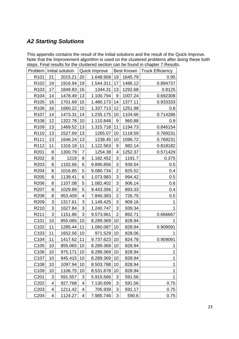
A2 Starting Solutions
This appendix contains the result of the Initial solutions and the result of the Quick Improve. Note that the Improvement algorithm is used on the clustered problems after doing these both steps. Final results for the clustered section can be found in chapter 7.Results.
Problem Initial solution Quick Improve Best Known Truck Efficiency
R101 21 2015.21 20 1.648.958 19 1645.79 0.95
R102 19 1916.94 19 1.544.311 17 1486.12 0.894737
R103 17 1849.83 16 1344.31 13 1292.68 0.8125
R104 14 1478.49 13 1.100.794 9 1007.24 0.692308
R105 16 1701.69 15 1.480.173 14 1377.11 0.933333
R106 16 1660.22 15 1.337.713 12 1251.98 0.8
R107 14 1473.31 14 1.235.175 10 1104.66 0.714286
R108 12 1322.78 10 1.110.848 9 960.88 0.9
R109 13 1469.52 13 1.315.718 11 1194.73 0.846154
R110 13 1527.69 13 1265.07 10 1118.59 0.769231
R111 13 1646.24 13 1238.45 10 1096.72 0.769231
R112 11 1316.18 11 1.122.563 9 982.14 0.818182
R201 8 1300.79 7 1254.38 4 1252.37 0.571429
R202 8 1219 8 1.182.452 3 1191.7 0.375
R203 8 1102.66 6 9.890.856 3 939.54 0.5
R204 8 1016.85 5 9.080.734 2 825.52 0.4
R205 8 1139.41 6 1.073.983 3 994.42 0.5
R206 8 1107.08 5 1.082.402 3 906.14 0.6
R207 8 1029.89 5 9.443.356 2 893.33 0.4
R208 8 953.409 4 7.840.383 2 726.75 0.5
R209 3 1317.61 3 1.149.425 3 909.16 1
R210 3 1627.84 3 1.240.747 3 939.34 1
R211 3 1151.86 3 9.573.961 2 892.71 0.666667
C101 10 855.065 10 8.289.369 10 828.94 1
C102 11 1285.44 11 1.060.087 10 828.94 0.909091
C103 11 1652.56 10 971.529 10 828.06 1
C104 11 1417.62 11 9.737.623 10 824.78 0.909091
C105 10 855.065 10 8.289.369 10 828.94 1
C106 10 975.171 10 8.289.369 10 828.94 1
C107 10 945.415 10 8.289.369 10 828.94 1
C108 10 1097.94 10 8.503.788 10 828.94 1
C109 10 1106.75 10 8.531.678 10 828.94 1
C201 3 591.557 3 5.915.566 3 591.56 1
C202 4 927.768 4 7.130.699 3 591.56 0.75
C203 4 1211.42 4 705.939 3 591.17 0.75
C204 4 1124.27 4 7.985.746 3 590.6 0.75
24
C205 3 627.918 3 6.270.945 3 588.88 1
C206 3 631.057 3 6.162.238 3 588.49 1
C207 4 745.767 3 6.461.871 3 588.29 1
C208 3 644.95 3 6.171.367 3 588.32 1
RC101 17 2108.46 17 1.715.033 14 1696.94 0.823529
RC102 16 1969.24 15 1.546.897 12 1554.75 0.8
RC103 14 1713.36 14 1.445.949 11 1261.67 0.785714
RC104 13 1658.36 12 1.286.674 10 1135.48 0.833333
RC105 18 1994.02 16 1.578.331 13 1629.44 0.8125
RC106 14 1715.06 13 1.437.741 11 1424.73 0.846154
RC107 14 1568.62 13 1.326.107 11 1230.48 0.846154
RC108 12 1543.85 12 1.320.572 10 1139.82 0.833333
RC201 5 2124.46 5 1.516.372 4 1406.91 0.8
RC202 4 1931.08 4 1.490.722 3 1367.09 0.75
RC203 4 1693.87 4 1.169.812 3 1049.62 0.75
RC204 4 1311.97 3 9.759.373 3 798.41 1
RC205 5 2007.99 5 1.407.424 4 1297.19 0.8
RC206 4 1716.24 4 1.381.135 3 1146.32 0.75
RC207 4 1737.11 4 1.301.147 3 1061.14 0.75
RC208 3 1361.24 3 1294.98 3 828.14 1 Table 5: Best found and best known results.
Problem Trucks Distance
R103 13 1292.68
R112 9 982.14
R201 4 1.253.234
R202 3 1.202.529
R204 2 856.364
R206 3 906.14
R207 2 894.889
R208 2 726.823
R209 3 921.659
R210 3 939.373
RC202 3 1370.92
RC203 3 1050.64
RC204 3 798.464
RC205 4 1297.65
RC206 3 1146.32
RC207 3 1.068.855
RC208 3 828.709 Table 6: Best found results by MACS.
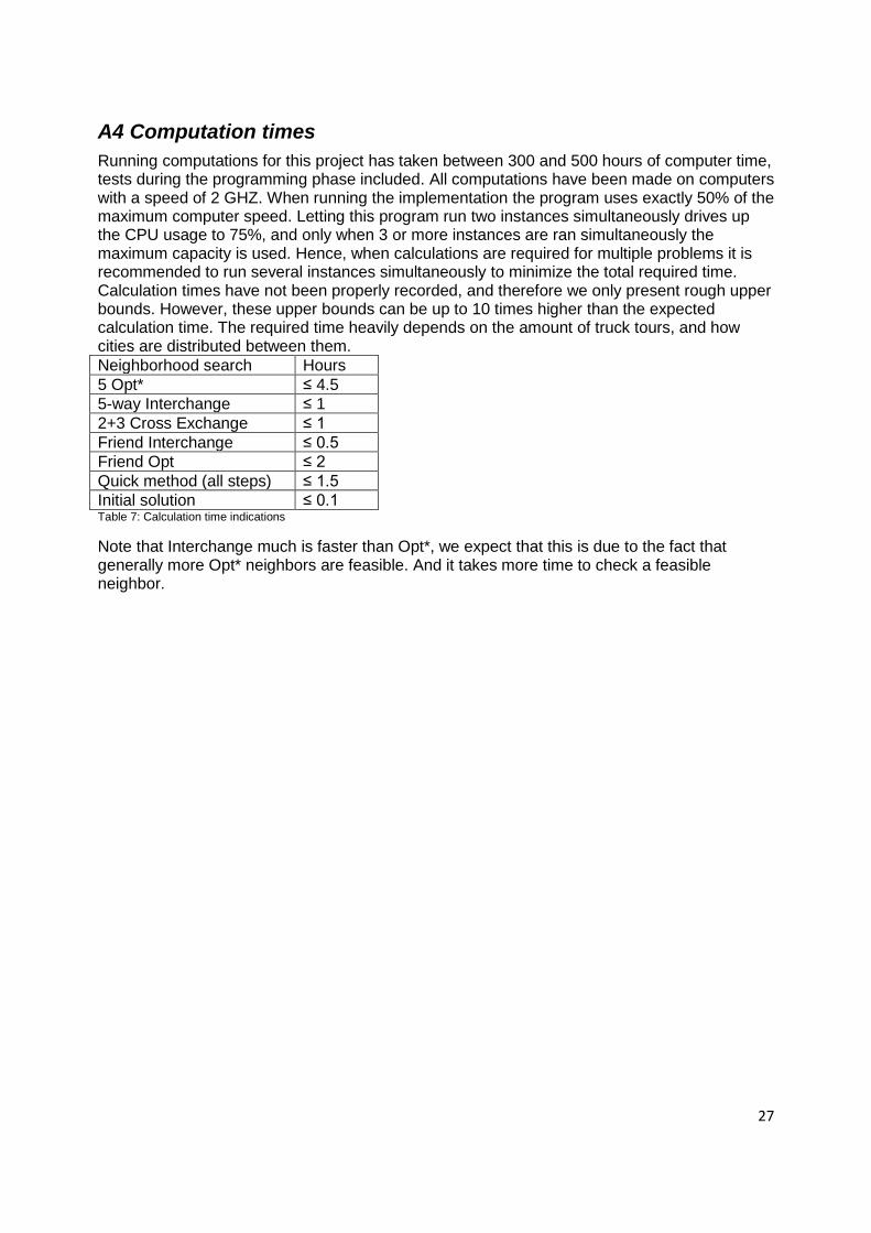
Running computations for this project has taken between 300 and 500 hours of computer time, tests during the programming phase included. All computations have been made on computers with a speed of 2 GHZ. When running the implementation the program uses exactly 50% of the maximum computer speed. Letting this program run two instances simultaneously drives up the CPU usage to 75%, and only when 3 or more instances are ran simultaneously the maximum capacity is used. Hence, when calculations are required for multiple problems it is recommended to run several instances simultaneously to minimize the total required time. Calculation times have not been properly recorded, and therefore we only present rough upper bounds. However, these upper bounds can be up to 10 times higher than the expected calculation time. The required time heavily depends on the amount of truck tours, and how cities are distributed between them.
Neighborhood search Hours
5 Opt* ≤ 4.5
5-way Interchange ≤ 1
2+3 Cross Exchange ≤ 1
Friend Interchange ≤ 0.5
Friend Opt ≤ 2
Quick method (all steps) ≤ 1.5
Initial solution ≤ 0.1 Table 7: Calculation time indications
Note that Interchange much is faster than Opt*, we expect that this is due to the fact that generally more Opt* neighbors are feasible. And it takes more time to check a feasible neighbor.