From Basic to Advanced PI Controllers: A Complexity vs ...cdn.intechopen.com/pdfs/19185.pdfAldo...

1. Introduction

The history of PIDs dates back to the beginning of the twentieth century when preliminaryworks of [Sperry (1922)] and [Minorski (1922)] provided mathematical results for the controlof the ship motion and of automatically steered bodies in general. In particular, Minorskiwas the first to introduce three-term controllers with Proportional-Integral-Derivative (PID)actions. The success of PID was fast and solid, as nowadays they still represent the mostpopular choice in most industrial process control applications. The main reasons for theirsuccess are:

• Reduced number of parameters: A process control engineer only has to tune a smallnumber of parameters to make the PID work effectively.

• Well-established tuning rules: There are predefined and well-known methods fordeciding the values of the PID regulators. The most popular methods were givenby [Ziegler and Nichols (1942)], [Astrom and Hagglund (1984)], and more recently[Zhuang and Atherton (1993)] and [Luyben and Eskinat (1994)]. Different tuning methodsare due to different control objectives (e.g. reference following, disturbance rejection) anddifferent plants (e.g. first-order model, second-order model).

• Good performances: The main reason for PID success is of course that good controlperformances are usually obtained; thus, the control engineer might not be interested indeveloping more complicated and less intuitive control schemes to improve somethingthat is already working fine.

The ideal equation of a PID controller is

uPID (t) = kp (r (t)− y (t)) + kp

{

∫ t

0

[

1

Ti(r (τ)− y (τ))

]

dτ + Tdd (r (t)− y (t))

dt

}

, (1)

where kp is the proportional gain, kp/Ti is the integral gain (sometimes denoted as ki) and kpTd

is the derivative gain (sometimes denoted as kd). According to conventional notation r(t), y(t)and u(t) denote respectively the reference, output and input signals. The error signal r(t)−y(t) is sometimes denoted as e(t). The classic feedback structure involving a PID controlleris shown in Figure 1. Equation (1) is sometimes considered an ideal equation for PIDs, as

From Basic to Advanced PI Controllers: A Complexity vs. Performance Comparison

Aldo Balestrino, Andrea Caiti, Vincenzo Calabró,

Emanuele Crisostomi and Alberto Landi

Department of Energy and Systems Engineering, University of Pisa

Italy

5

www.intechopen.com

2 Will-be-set-by-IN-TECH

Fig. 1. Classic Feedback PID Control Scheme

usually a few tricks are required to avoid some typical well-known problems associated withideal PIDs. For instance, a more realistic equation for PIDs is

uPID (t) = kp (b · r (t)− y (t)) + kp

{

∫ t

0

[

1

Ti(r (τ)− y (τ))

]

dτ − Tddy (t)

dt

}

, (2)

where the two main differences with the ideal equation (1) are the introduction of a set-pointweighting factor b [Rasmussen (2009)] and the absence of the reference in the derivative term.The term b is used to mitigate kicking phenomena, that usually occur when there is an abruptchange in the reference signal r(t). In the same circumstance, the derivative term of (1) is evenlarger, and a possible precaution is to relate the derivative only to the output signal. Assumingthat only piecewise constant reference signals should be followed, the derivative term of (2) isequal to that of (1) after the transient stage.Even the Equation (2) of a realistic PID is not always enough to obtain good controlperformances. One of the main drawbacks is that the PID’s parameters are fixed, thereforeif the plant’s parameters vary in time then the fixed PID can not always represent the optimalsolution. A simple way to deal with this problem is to use a relay auto-tuning procedure,i.e. the behaviour of the plant is continuously monitored, and the PID’s parameters areautomatically tuned in reaction to plant’s changes.A second drawback of conventional PIDs is that usually they are tuned either to have goodtracking performances or to have good disturbance rejection. Of course, in practice bothproperties are desirable at the same time, thus requiring the design of suitable filters thatseparate the high-frequency components of noise from the low-frequency components of thereference signal. Alternatively, it is possible to design two PIDs which are optimal with respectto reference tracking and disturbance rejection respectively, and a smart device that switchesbetween the two PIDs according to the most important objective in the particular moment.A last problem of PIDs is that an anti-windup scheme must be adopted, especially in thecommon case that the inputs to the actuators are bounded by physical constraints, see forinstance the tutorial [Peng et al. (1996)].A consequence of the previous remarks is that some modifications to the basic structure ofthe PIDs might be required to achieve better control performances. A classic improvement isobtained by considering PID-like regulators whose parameters are not fixed, but are allowedto be time variant to maintain good control performances in different operating conditions.Moreover, it is clear that time varying parameters introduce more degrees of freedom in thecontrol design, and in principle more flexibility in shaping the control response. Time variantPIDs can be designed according to several approaches well known in the literature: (a) fuzzyPIDs [Tang et al. (2001)]; in this case typically several fixed conventional PID controllers aredesigned for different operating conditions, and are then interpolated according to a set offuzzy logic rules. Alternatively, fuzzy rules are used only to improve one component of thePID, for instance the set-point weighting term as in [Visioli (2004)]. (b) nonlinear PIDs; see

86 Advances in PID Control

www.intechopen.com

From Basic to Advanced PI Controllers: a Complexity vs. Performance Comparison 3

for instance [Haj-Ali and Ying (2004)] for a comparison with fuzzy PIDs. (c) variable structurePIDs, see for instance [Scottedward Hodel and Hall (2001)] or [Visioli (1999)] where a classicPID is modified by adding a feedforward term.In this spirit, this work compares a traditional PI with three parameter varying PIs,characterised by an increasing level of complexity. As a support to the evalution of the controlperformance of each of the four regulators, conventional control indices, such as the integralof the absolute value or the square of the error signal, and the integral of the absolute valueof the input and its derivative, have been used, as further detailed in Section 4. The finalobjective is to establish some thumb rules that quantify how much (or when) it is convenientto complicate the original conventional PI, in terms of improved control performances.

The discussion in this paper is restricted to PIs rather than PIDs for two main reasons:

• Many industrial controllers are simple PIs.

• The design of the derivative action simply follows the design of the other components.Therefore the derivative component can be introduced without affecting the general resultsof this work. Simple rules to introduce the derivative component can be found in the recentreference [Leva and Maggio (2011)].

Furthermore, the discussion is here restricted to linear time invariant systems, as in practicemost industrial plants can be represented in such a form, eventually after a linearisationstep around the desired operating point. While PI are successful in most stabilization andcontrol problems, from a theoretical perspective there is a class of linear systems which arenot stabilizable via output PI feedback; however, such examples will not be trated in thischapter.This paper is organised as follows: next section introduces the 3 PIs that will be thoroughlycompared with a conventional PI in benchmark examples. Section 3 illustrates the tuningprocedures for all PIs. Section 4 compares the PI regulators in a challenging noisy referencetracking example, while Section 5 is dedicated to a realistic example. In the last section finalconclusions are given and future work is outlined.

2. PI-like regulators

This sections presents the four regulators that will be later compared in challenging controlproblems.

2.1 Conventional PI controller

The conventional PI is described by Equation 1, without the derivative term, i.e.

uPI (t) = kp (b · r (t)− y (t)) + kp

{

∫ t

0

[

1

Ti(r (τ)− y (τ))

]

dτ

}

, (3)

where all parameters are constant.

2.2 Variable Integral PI

A simple modification of the standard PI was proposed in [Balestrino et al. (2009)] and is herereproposed as a term of comparison as it represents a good trade-off between performances

87From Basic to Advanced PI Controllers: A Complexity vs. Performance Comparison

www.intechopen.com


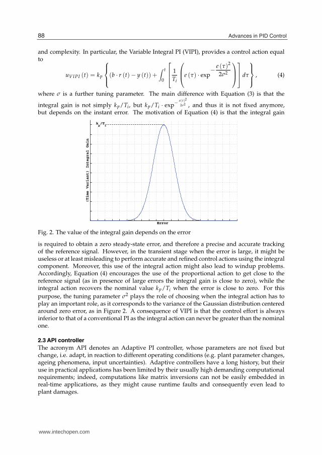
and complexity. In particular, the Variable Integral PI (VIPI), provides a control action equalto

uVIPI (t) = kp

⎧

⎪

⎨

⎪

⎩

(b · r (t)− y (t)) +∫ t

0

⎡

⎢

⎣

1

Ti

⎛

⎜

⎝e (τ) · exp

−e (τ)2

2σ2

⎞

⎟

⎠

⎤

⎥

⎦dτ

⎫

⎪

⎬

⎪

⎭

, (4)

where σ is a further tuning parameter. The main difference with Equation (3) is that the

integral gain is not simply kp/Ti, but kp/Ti · exp− e(τ)2

2σ2 , and thus it is not fixed anymore,but depends on the instant error. The motivation of Equation (4) is that the integral gain

Error

(Time Variant) Integral Gain

kp/T

i

Fig. 2. The value of the integral gain depends on the error

is required to obtain a zero steady-state error, and therefore a precise and accurate trackingof the reference signal. However, in the transient stage when the error is large, it might beuseless or at least misleading to perform accurate and refined control actions using the integralcomponent. Moreover, this use of the integral action might also lead to windup problems.Accordingly, Equation (4) encourages the use of the proportional action to get close to thereference signal (as in presence of large errors the integral gain is close to zero), while theintegral action recovers the nominal value kp/Ti when the error is close to zero. For this

purpose, the tuning parameter σ2 plays the role of choosing when the integral action has toplay an important role, as it corresponds to the variance of the Gaussian distribution centeredaround zero error, as in Figure 2. A consequence of VIPI is that the control effort is alwaysinferior to that of a conventional PI as the integral action can never be greater than the nominalone.

2.3 API controller

The acronym API denotes an Adaptive PI controller, whose parameters are not fixed butchange, i.e. adapt, in reaction to different operating conditions (e.g. plant parameter changes,ageing phenomena, input uncertainties). Adaptive controllers have a long history, but theiruse in practical applications has been limited by their usually high demanding computationalrequirements; indeed, computations like matrix inversions can not be easily embedded inreal-time applications, as they might cause runtime faults and consequently even lead toplant damages.


www.intechopen.com


More recently, adaptive techniques have been applied to PI controllers, as their simplestructure is very attractive, by including additional adaptive terms to extend and robustifysuch controllers. One example is given by [Fisher (2009)], where the authors compare threedifferent controllers: a classic PI, an Adaptive PI and a P-FI which is a Proportional+FuzzyIntegral term controller. In this paper, we use the second controller (API) as a term ofcomparison in our examples, because it is characterised by accurate and robust trackingperformances. The main property of adaptive controllers is that parameters are not fixed,but vary in time searching for an optimal configuration. In [Fisher (2009)] the controllerparameters update law is described by

kp = −γpkp + βpe2 (5)

ki = −γiki + βie∫ t

0e(τ)dτ (6)

with positive constant parameters γp, γi, βp , βi; the resulting control law is as usual

uAPI(t) = kpe(t) + ki

∫ t

0e(τ)dτ (7)

The rationale of this adaptive PI control is that the updating law is composed by a

dissipative term

{

−γpkp

−γiki(8)

and an

anti-dissipative term

{

βpe2

βie∫ t

0 e(τ)dτ. (9)

The dissipative term is used to decrease the value of the corresponding gain, once that theanti-dissipative terms becomes small. For instance, a large error will cause an increase of theproportional gain through the anti-dissipative term; thus the error will decrease, and whenclose to zero (e ≈ 0), the proportional gain decreases exponentially with decay rate γp.

2.4 FAPI controller

Similarly to many other recent approaches, we also propose here a Fuzzy variant of theAdaptive PI (FAPI). Fuzzy approximation property has been widely and successfully usedin robotics and control theory, to handle model uncertainties and external unpredictabledisturbances. A large number of controllers use the Wang universal approximation theorem[Wang (1997)], to design nonlinear integral terms to improve performance indices and addressrobustness issues. However, in many cases, as shown in [Fisher (2009)], the involvedadditional computational efforts do not match significative performance improvements, thusnot making fuzzy techniques particularly attractive.Here we present a different novel approach to fuzzy controllers, where the simplicity of theconventional PI regulator, the interesting idea of the VIPI integral action and the robustnessproperties of adaptive PI controllers, are all combined together into a single Fuzzy-AdaptivePI Control (FAPI).Next section is dedicated to recall the basic ideas of Fuzzy Logic Theory that, in the followingsection, will be used to implement the FAPI controller, which is one of the main contributionsof this paper.


www.intechopen.com


2.4.1 Fuzzy logic theory background

A fuzzy set A on a domain X is a set defined by the membership function μA(x) which is amapping from the domain X into the unit interval:

μA(·) : X → [0, 1]. (10)

There are several ways to define a fuzzy set, in particular we define it here using the analyticdescription of its membership function μA(x) = f (x). For instance (see Fig. 3), the triangularmembership function can be described as:

μ(x; a, b, c) = max

(

0, min

(

x − a

b − a, 1,

c − x

c − b

))

(11)

where a,b and c are parameters that is related to the coordinates of the triangle’s vertices,whereas a Gaussian membership function can be described as

μ(x; η, σ) = exp

[

−

(

x − η

σ

)2]

. (12)

A static or dynamic system which makes use of fuzzy sets and the correspondingmathematical framework is called a fuzzy system. In order to derivate the FAPI controller

−2 −1.5 −1 −0.5 0 0.5 1 1.5 20

0.1

0.2

0.3

0.4

0.5

0.6

0.7

0.8

0.9

1

x

µ(x)

Membership Functions

Triangular

Gaussian

Fig. 3. Example of Membership Functions: Triangular (a = −1, b = −0.5, c = 0) andGaussian (η = 0.5, σ = 0.4)

updating law, it is necessary to define the intersection of fuzzy sets (connective AND) ,obtained by considering a function t : [0, 1] × [0, 1] → [0, 1] that transforms the membershipfunctions of fuzzy sets A and B into the membership function of the intersection of A and B,that is:

t [μA(x), μB(x)] = μA∩B(x). (13)

A function t can be qualified as an intersection function, if it satisfies at least the followingfour requirements:

t(0, 0) = 0, t(a, 1) = t(1, a) = a boundary conditiont(a, b) = t(b, a) commutativity

t(a, b) ≤ t(a′, b′), ∀a ≤ a′, b ≤ b′ monotonicityt(t(a, b), c) = t(a, t(b, c)) associativity

. (14)


www.intechopen.com


In the following analysis, the probabilistic connective AND will be used:

μA∩B(x) = μA(x)μB(x). (15)

The most common fuzzy systems are defined by means of if-then rules: rule-based fuzzysystems. In the rule-based fuzzy systems, the relationships between variables are representedin the following general form:

if antecedent proposition then consequent proposition.

A fuzzy proposition is a statement like "x is big" where "big" is a linguistic label, defined by afuzzy set on the universe of discourse of variable x. In the linguistic fuzzy model developedby [Zadeh (1978)] and [Mamdani (1977)], both the antecedent and the consequent are fuzzypropositions:

Ri : if x is Ai then y is Bi , i = 1, ..., L, (16)

where L is the number of propositions (rules). Here x is the input (antecedent) linguisticvariable, and Ai are the antecedent linguistic terms (labels). Similarly, y is the output(consequent) linguistic variable and Bi are the consequent linguistic terms. The linguisticterms Ai,Bi are always fuzzy sets. After fuzzy theory gained popularity, many controlproblems have been recasted into control of Takagi-Sugeno-Kang (TSK) models:

Ri : if x is Ai then y = fi(x) , i = 1, ..., L (17)

which is a particular case of the general fuzzy model (16), obtained when the consequentfuzzy sets Bi are functions of the variable x. In systems and control theory, TSK models arefrequently used to model nonlinear systems over a fuzzy space. The resulting TSK modelcan efficiently clone the nonlinear system or alternatively, approximate it over a defineddomain. For such a nonlinear systems representation, stability and synthesis of controllersand observers can be expressed in terms of Linear Matrix Inequalities, which in turn can besolved adopting convex optimization techniques as shown in [Tanaka (2001)]. It is importantto mention that the output of a fuzzy system can be obtained using different defuzzificationmethods. In the remainder of this chapter we will use the following TSK model:

Ri : if x1 is Ai1 and ... xn is Ain then y = fi(x) , i = 1, ..., L (18)

where we consider that each rule has an antecedent proposition obtained by intersecting nfuzzy sets. The output can be evaluated by considering the Center of Gravity defuzzificationmethod

y =L

∑i=1

αi fi(x) (19)

where

α(t) = (α1(t), ..., αL(t)), αi(t) =βi(t)

∑Li=1 βi(t)

,

βi(t) =n

∏j=1

μAij(x). (20)


www.intechopen.com


2.4.2 FAPI parameters update law

According to the discussion on fuzzy sets and rules introduced in the previous section, weintroduce now the controller parameters update laws:

IF error is SMALL, then kp = −βpkp (21)

IF error is MEDIUM, then kp = −γp(kp − k∗p) (22)

IF error is LARGE, then kp = αpk∗pe2 (23)

for the proportional gain kp, while for the integral action we have

IF error is LARGE, then ki = −βiki (24)

IF error is MEDIUM, then ki = −γi(ki − k∗i ) (25)

IF error is SMALL, then ki = αik∗i e∫ t

0e(τ)dτ. (26)

The main difference with respect to the API regulator is the presence of the two terms k∗p andk∗i that are the gains of a reference model regulator K∗. In order to compute the correspondingtime-varying gain, we will consider a single Gaussian membership function μS(e) definedover the error domain to identify the fuzzy set SMALL (S), and also the fuzzy sets MEDIUM(M) and LARGE (L) as follows:

μS = e−(xσ )

2

, μL(e) = 1 − μS(e), μM(e) = μS∩L(e) = μS(e) · μL(e) (27)

The philosophy of shaping the control effort on the basis of the error value is analogous tothat of the previously introduced VIPI. The resulting kp gain law is obtained as

kp =1

1 + μM(e)

(

αpμL(e)k∗pe2 − βpμS(e)kp − γpμM(e)(kp − k∗p)

)

(28)

while the integral gain ki law is

ki =1

1 + μM(e)

(

αiμS(e)k∗i e∫ t

0e(τ)dτ − βiμL(e)ki − γiμM(e)(ki − k∗i ).

)

(29)

Each updating law it is composed of three terms:

dissipative term

{

−βpμS(e)kp

−βiμL(e)ki(30)

used to decrease the (absolute) value of the gains,

anti-dissipative term

{

αpμL(e)k∗pe2

αiμS(e)k∗i e∫ t

0 e(τ)dτ(31)

used to increase the gain values analogously to the API control philosophy, and

model reference tracking term

{

−γpμM(e)(kp − k∗p)

−γiμM(e)(ki − k∗i )(32)


www.intechopen.com


used to force the adapting law to generate controller gains sufficiently close to the idealcontroller K∗. In the end, the control law is as usual

uFAPI(t) = kpe(t) + ki

∫ t

0e(τ)dτ (33)

In practice, when the error is large, the parameter update laws make the proportional gainincrease due to its anti-dissipative term, while the integral action progressively disappears.This leads to a fast response (high proportional gain). On the other hand, when the error issmall, the proportional gain is subject to the dissipative term and gets negligible values, whilethe integral component grows. This will result in a disturbance rejection behaviour. In anymoment, good performances are guaranteed by the third term that makes the PI close to themodel reference controller K∗.Remark: Both the API controller developed in [Fisher (2009)] and the FAPI controller shownhere are not symmetrical with respect to the error signal as their update rules are a functionof the error, and thus depend on its sign. As a consequence, they can behave differently if thereference signal is larger or smaller than the actual output of the plant.

3. Tuning methods

3.1 Tuning of the conventional PI

In this paper we tune the conventional PI using Zhuang-Atherton optimal parameters[Zhuang and Atherton (1993)]. In particular we use the values of Table 1 of[Zhuang and Atherton (1993)], which correspond to PI tuning formulae for set-point changesin the case of first-order plus dead time plant model, optimised in order to minimise theIntegral of the Square Error (ISE) signal. The set-point weighting factor is usually not used(i.e. b = 1), as in the examples a time-varying reference signal is used.

3.2 Tuning of the VIPI

Tuning of the VIPI is a two-step procedure:

1. Conventional tuning is first performed, and values of kp and Ti are found according to theprocedure outlined in Section 3.1.

2. The further parameter σ is computed to decide at which point the integral action shouldcome into action. Namely, the integral action must already be active when the error isequal to the steady-state error obtained using only the proportional action.

Example :Let us consider a plant described by the transfer function

G(s) =4

s2 + 4s + 4(34)

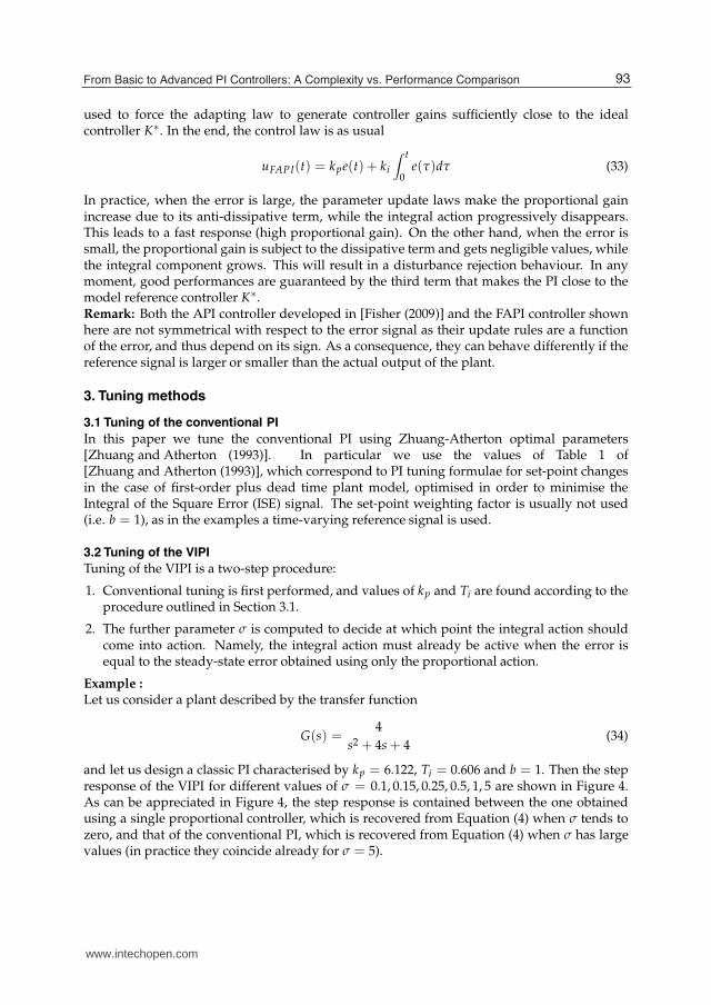
and let us design a classic PI characterised by kp = 6.122, Ti = 0.606 and b = 1. Then the stepresponse of the VIPI for different values of σ = 0.1, 0.15, 0.25, 0.5, 1, 5 are shown in Figure 4.As can be appreciated in Figure 4, the step response is contained between the one obtainedusing a single proportional controller, which is recovered from Equation (4) when σ tends tozero, and that of the conventional PI, which is recovered from Equation (4) when σ has largevalues (in practice they coincide already for σ = 5).


www.intechopen.com


0 1 2 3 4 5 6 7 8 9 100

0.5

1

1.5

Time (s)

ucontroller

Solid line: Conventional PI and single P

Dashed line: σ = 0.1, 0.15, 0.25, 0.5, 1, 5

Fig. 4. Different step responses as a function of the free parameter σ of the VISI. The stepresponse is contained between the one obtained using a single proportional controller (i.e.σ → 0) and high values of the parameter. In this case, the step response when σ = 5 alreadycoincides with the one obtained with the nominal PI.

3.3 Tuning of the API

Tuning of adaptive controllers is simpler than other PIs as the inner adaptive capacity allowsthe API to recover good performances against non optimal initial tunings. However, APIsare characterised by more degrees of freedom, e.g. parameters in the updating rules. For thepurpose of the example shown in the following sections, the adaptive PI control parametersγ and β have been optimally tuned (using genetic algorithms) in order to get a goodtrade-off between tracking and disturbance rejection. Particular care is required to handlethe anti-dissipative terms, which might yield to instability problems when a fault occurs. Infact, the anti-dissipative term should be neglected only when the error is close to zero.

3.4 Tuning of the FAPI

The FAPI controller parameters α, β, γ must be tuned, after a desired target controller K∗ ischosen. In this case, we use a conventional PI tuned according to Zhuang-Atherton rules (seeSection 3.1) as a reference model. Then, the parameters can be tuned keeping in mind thateach parameter directly affects a different controller property:

• α: Adapting

• β: Low Gain Trend

• γ: K∗ Model Reference Tracking.

Therefore, parameters are chosen in function of whether the priority objective is fast responseto variations, or no overshoots or adherence to the ideal model controller. Particular careshould be used in tuning α, that should be small in presence of significative system delays.

4. Comparison of the four PIs

As a preliminary comparison the step-responses of the four controllers are compared. Then,in the following sections, a more challenging example and a realistic scenario are simulatedto further establish the differences among the proposed PI regulators. The step response of


www.intechopen.com


the four controllers is shown in Figure 5, in the case of the system plant (34). The showncomparison is performed after a transient time given to the adaptive controllers to adapttheir parameters, and after Zhuang-Atherton tuning procedure for the other two controllers[Zhuang and Atherton (1993)]. The control performances of the four regulators are also

0 1 2 3 4 5 6 7 8 9 10−0.2

0

0.2

0.4

0.6

0.8

1

1.2

1.4

1.6

Ti ( )

y(t)

Reference Signal

PI

VIPI

API

FAPI

Fig. 5. Comparison of the four PI controllers in terms of the step response.

compared in Table 1 to further distinguish and classify the proposed regulators, where thefollowing well known control indices were used

• IAE: Integral of the Absolute value of the Error, IAE =∫ t

0 |e(τ)| dτ

• ISE: Integral of the Square Error, ISE =∫ t

0 (e(τ))2 dτ

• IAU: Integral of the Absolute value of the input u , IAU =∫ t

0 |u(τ)| dτ

• IADU: Integral of the Absolute value of the Derivative of the input u , IADU =∫ t

0

∣

∣

∣

du(τ)dτ

∣

∣

∣dτ

IAE ISE IAU IADU

PI 0.58 0.26 16.75 22.20

VIPI 0.46 0.21 16.10 18.42API 0.54 0.32 15.59 11.72

FAPI 0.50 0.27 15.47 8.69

Table 1. Comparison of the four controllers in terms of the Step Response. The best values ofthe indices have been highlighted in grey. The FAPI requires the least control effort, while theVIPI has the best overall control performances.

4.1 A more challenging example

The performances of the four controllers are again compared in a more challenging scenariowhere the plant transfer equation is the same (i.e. Equation (34)), but the reference signalis composed of a periodic sinusoidal component and of a pulse wave, plus a filteredGaussian random signal n(t) added to simulate sensor noise (i.e. e(t) = r(t)− y(t)− n(t)).As a consequence, this simulation is tailored on purpose to compare the robustness and


www.intechopen.com


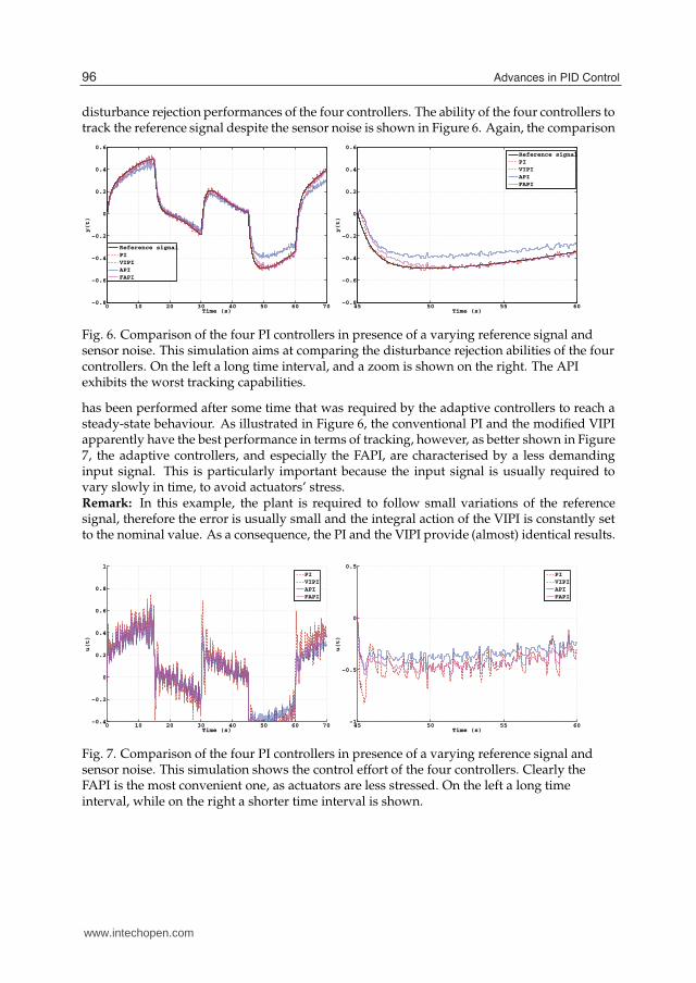
disturbance rejection performances of the four controllers. The ability of the four controllers totrack the reference signal despite the sensor noise is shown in Figure 6. Again, the comparison

0 10 20 30 40 50 60 70−0.8

−0.6

−0.4

−0.2

0

0.2

0.4

0.6

Time (s)

y(t)

Reference signal

PI

VIPI

API

FAPI

45 50 55 60−0.8

−0.6

−0.4

−0.2

0

0.2

0.4

0.6

Time (s)

y(t)

Reference signal

PI

VIPI

API

FAPI

Fig. 6. Comparison of the four PI controllers in presence of a varying reference signal andsensor noise. This simulation aims at comparing the disturbance rejection abilities of the fourcontrollers. On the left a long time interval, and a zoom is shown on the right. The APIexhibits the worst tracking capabilities.

has been performed after some time that was required by the adaptive controllers to reach asteady-state behaviour. As illustrated in Figure 6, the conventional PI and the modified VIPIapparently have the best performance in terms of tracking, however, as better shown in Figure7, the adaptive controllers, and especially the FAPI, are characterised by a less demandinginput signal. This is particularly important because the input signal is usually required tovary slowly in time, to avoid actuators’ stress.Remark: In this example, the plant is required to follow small variations of the referencesignal, therefore the error is usually small and the integral action of the VIPI is constantly setto the nominal value. As a consequence, the PI and the VIPI provide (almost) identical results.

0 10 20 30 40 50 60 70−0.4

−0.2

0

0.2

0.4

0.6

0.8

1

Time (s)

u(t)

PI

VIPI

API

FAPI

45 50 55 60−1

−0.5

0

0.5

Time (s)

u(t)

PI

VIPI

API

FAPI

Fig. 7. Comparison of the four PI controllers in presence of a varying reference signal andsensor noise. This simulation shows the control effort of the four controllers. Clearly theFAPI is the most convenient one, as actuators are less stressed. On the left a long timeinterval, while on the right a shorter time interval is shown.


www.intechopen.com


4.2 A realistic example: Ship course control

Let us consider a 3DoF model of a low-speed marine vessel [Fossen (2002)]:

Mν + C(ν)ν + Dν = τ + JT(η)τd (35)

η = J(η)ν (36)

where

• M represents the generalized mass-inertia matrix, including the added-massescontribution

• C(ν) contains the Coriolis-centripetal effects

• D represent the linear approximation of hydrodynamic drag

• τ is the generalized force-torque applied to the 3DoF model expressed in the body-fixedreference frame

• τd is an external disturbance expressed in the navigation referenceframe

• ν = [u, v, r]T ∈ R3 is the state variable related to the surge, sway and yaw rate speed

• η = [pn, pe, ψ] ∈ R3 represents the position and the orientation of the vessel with respect

to the navigation frame

• J(η) is the Jacobian matrix which relates body-fixed reference frame to navigation referenceframe:

J(η) =

⎡

⎣

cos ψ − sin ψ 0sin ψ cos ψ 0

0 0 1

⎤

⎦ (37)

Let us assume that the vessel is moving at constant speed u0 , and√

u20 + v2 ≈ u0, then

the previous 3DoF model can be decoupled into longitudinal and manoeuvring subsystems.Here we will analyse the manoeuvring subsystem in order to obtain a course control for avessel equipped with a single rudder. For low surge speed, in addition the Eq. (35) can beapproximated by:

M ˙ν + N(u0)ν = bδ (38)

where ν = [v, r]T, b = −[Yδ, Nδ]T ∈ R

2 and

M =

[

m − Yv mxg − Yr

mxg − Yr Iz − Nr

]

, N(u0) =

[

−Yv mu0 − Yr

−Nv mxgu0 − Nr

]

(39)

where the parameters Yδ, Nδ are used to model the force and the torque generated by therudder, Yv, Yr, Nr are parameters related to the added-masses, m, xg, Iz are parameter of therigid-body (mass, center of gravity and moment of inertia, respectively), Yv, Yr, Nv, Nr arecoefficients related to the drag effects and δ is the rudder deflection. The equivalent state-spacemodel of (38) can be found by observing that:

˙ν = −M−1N(u0)ν + M−1bδ = Aν + Bδ (40)

Considering the the parameters of the CyberShip II experimentally estimated in Fossen (2004),choosing a constant speed of u0 = 1.5m/s ≈ 3knots and defining the output y = r =


www.intechopen.com


Cr ν, Cr = [0, 1] ∈ R2, the following second linear time invariant system, also referred as

Nomoto 2nd order model is obtained:

Gr(s) = Cr (sI − A)−1 B =r(s)

δ(s)=

−0.09185s − 0.002137

s2 + 0.8165s + 0.04882(41)

Since the course angle derivative is related to the yaw-rate as ψ = r, we can finally derive thecourse model for the CyberShip II as:

Gψ(s) =ψ(s)

δ(s)=

1

sGr(s) =

−0.09185s − 0.002137

s3 + 0.8165s2 + 0.04882s(42)

The controller parameters used in the course-control problem are summarised in Table 2.

ZA VIPI API FAPI

K∗p 7.7220 7.7220 - 7.7220

K∗i = K∗

p/T∗i 0.0978 0.0978 - 0.0978

σ - 0.5 - 0.25

βp - - 1.1612 0.0087

βi - - 1.1343 0.1206γp - - 0.0151 0.1142

γi - - 0.1363 0.1671αp - - - 0.0011

αi - - - 0.7126

Table 2. Course Control Problem: controller parameters used in the simulation.

Note that we are not handling actuator saturations and limitations of the input rate.However, in order to use efficiently those controllers with such limitations the adoption ofanti-windup systems and reference filters is strongly recommended. In practice, the use ofa frequency-shaped reference signal causes a smoother and less demanding control actionwhich is expected to satisfy the actuator limitations.The four controllers are compared in the challenging scenario described in Figure 8. In thissimulation we assume that the reference signal is a desired course angle (i.e. not a stepreference, as it is not realistic in this context as previously remarked). Disturbance is modeledwith two components: a filtered Gaussian noise, of the order of 2− 3◦; and an aperiodic squarepulse which refers to unpredictable external disturbance (e.g. wave current, wind gust). Itis possible to note from Figure 8 that the API controller not always provide a satisfactorytracking of the reference signal. On the other hand, the other controllers have similar goodperformances, but the FAPI is characterised by a reduced control effort.

5. Conclusion

This chapter gives a comparison between a conventional PI regulator tuned according toZhuang-Atherton rules with three less conventional controllers: a variable integral componentPI (VIPI), an adaptive PI (API) and a fuzzy adaptive PI (FAPI). The VIPI is characterised byone time variant parameter, i.e. the integral one, and only one more degree of freedom (theparameter σ). Both the API and the FAPI have two time variant parameters and more degreesof freedom, as for instance the dissipative and anti-dissipative coefficients that regulate theparameters’ update laws.


www.intechopen.com


0 20 40 60 80 100 120 140−30

−20

−10

0

10

20

30

40

50

Time (s)

Course Angle

ψ (deg)

Reference signal

PI

VIPI

API

FAPI

0 20 40 60 80 100 120 140−80

−60

−40

−20

0

20

40

60

80

Time(s)

Rudder Deflection

δ(t) (deg)

PI

VIPI

API

FAPI

Fig. 8. Comparison of the four PI controllers in response to a course angle reference signal(on the left). Realistic disturbances are taken into consideration. On the right, the controleffort of the four controllers.

Simulations show that the VIPI generally outperforms the simple PI both in terms of thecontrol effort, which is always inferior, and in terms of settling time. The VIPI is veryconvenient, as it only contains one more parameter than the conventional PI, and betterperformances are usually achieved without requiring a complex tuning procedure for theextra parameter. On the other hand, the adaptive controllers require a more laborious tuningprocedure (as more parameters are involved), and not always the control performance isso satisfactory, especially for the API, at least for the proposed examples. However, theFAPI, although provides similar control results to the PI and the VIPI, is characterised by areduced small effort, both in terms of the absolute value and its derivative; for this reason it isparticularly suitable in particular control applications: for instance when control componentswith moving parts are involved (e.g. valves) frequent fluctuations of the control action shouldbe avoided to skip the high expenses of valve wear and maintenance programs.Ongoing and future work will follow several directions:

• Robustness performances will be further investigated, so to account for time variantprocess plants. In some industrial applications, the plant coefficients change accordingto different factors (e.g. temperature, age, wear and tear of the machines).

• The controllers can be further compared on their ability to prevent wind-up phenomena.

• The proposed framework can be easily extended to decentralised Multiple Input MultipleOutput (MIMO) control problems.

• The FAPI controller exhibits the best performance in terms of control effort, and for thisreason it will be used in a real application in underwater robotics.

6. References

E. Sperry, Automatic steering, Society of Naval Architects and Marine Engineers, 1922.N. Minorski, Directional stability of automatically steered bodies, Journal of American Society of

Naval Engineers, 1922.J. Ziegler and N. Nichols, Optimum settings for automatic controller, Trans. ASME, vol. 75,

pp.827–833, 1942.K. Astrom and E. Hagglund, Adaptive tuning of simple regulators with specifications on phase and

amplitude margins, Automatica, vol. 20, pp. 645–651, 1984.


www.intechopen.com


M. Zhuang and D.P. Atherton, Automatic tuning of optimum PID controllers, IEE Proceedings Don Control Theory and Applications, vol. 140, pp. 216–224, 1993.

W. Luyben and E. Eskinat, Nonlinear auto-tune identification, International Journal of Control,vol. 59, pp.595–626, 1994.

H. Rasmussen, Automatic tuning of pid-regulators, Textbook, Department of ControlEngineering, Aalborg University, Denmark, 2009.

Y. Peng, D. Vrancic and R. Hanus, Anti-windup, bumpless, and CT techniques for PID controllers,IEEE Control systems magazine, vol. 16, pp.48–56, 1996.

K. Tang, K. Man, G. Chen and S. Kwong, An optimal fuzzy PID controller, IEEE Transactions onIndustrial Electronics, vol. 48, pp. 757–765, 2001.

A. Visioli, A new design for a PID plus feedforward controller, Journal of Process Control, vol. 14,pp. 457–463, 2004.

A. Haj-Ali and H. Ying, Structural analysis of fuzzy controllers with nonlinear input fuzzy sets inrelation to nonlinear PID control with variable gain, Automatica, vol. 40, pp. 1551–1559,2004.

A. Scottedward Hodel and C.E. Hall, Variable-Structure PID control to prevent integrator windup,IEEE Transactions on Industrial Electronics, vol. 48, no. 2, 2001.

A. Visioli, Fuzzy logic based set-point weight tuning of PID controllers, IEEE Transactions onSystems, Man, and Cybernetics - Part A, vol. 29, no. 6, pp. 587–592, 1999.

A. Leva and M. Maggio, A systematic way to extend ideal PID tuning rules to the real structure,Journal of Process Control, vol. 21, pp. 130–136, 2011.

A. Balestrino, V. Biagini, P. Bolognesi and E. Crisostomi, Advanced variable structure PIcontrollers, IEEE Conference on Emerging Technologies and Factory Automation(ETFA), 2009.

A.D. Fisher, J.H. VanZwieten and T.S. VanZwieten, Adaptive Control of Small Outboard-PoweredBoats for Survey Applications, OCEANS 2009, MTS/IEEE Biloxi - Marine Technologyfor Our Future: Global and Local Challenges, 2009.

L.X. Wang, A Course in Fuzzy Systems and Control, Prentice Hall,1997.L.A. Zadeh, Fuzzy Sets as basis for a theory of possibility., Fuzzy Sets and System 1, 1978.E.H. Mamdani, Application of Fuzzy Logic to Approximate Reasoning Using Linguistic Synthesis,

IEEE Transaction on Computers, 1977.K. Tanaka and H.O. Wang, Fuzzy Control Systems Design and Analysis: A Linear Matrix Inequality

Approach, John Wiley and Sons, 2001.T.I. Fossen, Marine Control Systems: Guidance, Navigation and Control of Ships, Rigs and

Underwater Vehicles, Marine Cybernetics, 2002.T. I. Fossen, Modeling, Identification, and Adaptive Maneuvering of CyberShip II: A complete design

with experiments, Proc. of the IFAC CAMS’04, Ancona, Italy.


www.intechopen.com

Advances in PID ControlEdited by Dr. Valery D. Yurkevich

ISBN 978-953-307-267-8Hard cover, 274 pagesPublisher InTechPublished online 06, September, 2011Published in print edition September, 2011

InTech EuropeUniversity Campus STeP Ri Slavka Krautzeka 83/A 51000 Rijeka, Croatia Phone: +385 (51) 770 447 Fax: +385 (51) 686 166www.intechopen.com

InTech ChinaUnit 405, Office Block, Hotel Equatorial Shanghai No.65, Yan An Road (West), Shanghai, 200040, China

Phone: +86-21-62489820 Fax: +86-21-62489821

Since the foundation and up to the current state-of-the-art in control engineering, the problems of PID controlsteadily attract great attention of numerous researchers and remain inexhaustible source of new ideas forprocess of control system design and industrial applications. PID control effectiveness is usually caused by thenature of dynamical processes, conditioned that the majority of the industrial dynamical processes are welldescribed by simple dynamic model of the first or second order. The efficacy of PID controllers vastly falls incase of complicated dynamics, nonlinearities, and varying parameters of the plant. This gives a pulse to furtherresearches in the field of PID control. Consequently, the problems of advanced PID control system designmethodologies, rules of adaptive PID control, self-tuning procedures, and particularly robustness and transientperformance for nonlinear systems, still remain as the areas of the lively interests for many scientists andresearchers at the present time. The recent research results presented in this book provide new ideas forimproved performance of PID control applications.

How to referenceIn order to correctly reference this scholarly work, feel free to copy and paste the following:

Aldo Balestrino, Andrea Caiti, Vincenzo Calabro , Emanuele Crisostomi and Alberto Landi (2011). From Basicto Advanced PI Controllers: A Complexity vs. Performance Comparison, Advances in PID Control, Dr. Valery D.Yurkevich (Ed.), ISBN: 978-953-307-267-8, InTech, Available from:http://www.intechopen.com/books/advances-in-pid-control/from-basic-to-advanced-pi-controllers-a-complexity-vs-performance-comparison

Date post:	23-May-2018
Category:	Documents
Upload:	ngocong
View:	220 times
Download:	1 times

From Basic to Advanced PI Controllers: A Complexity vs ...cdn.intechopen.com/pdfs/19185.pdfAldo...

Documents