From Crisis to IMF-Supported Program:

Politics and the speed required by financial markets

Ashoka Mody and Diego Saravia1

Abstract

We examine the time span between the onset of a financial crisis and the agreement on an IMF-supported adjustment program. This span appears to have decreased over time, even before the rapidly concluded programs following the subprime crisis. More precisely, we find that the time from a crisis to the negotiation of a program has been smaller the more serious the crisis, responding to a widening range of financial vulnerabilities with the growing financial integration and threat of contagion. Politics—both in the international governance of the IMF and in domestic collective action—have been sensitive to time pressures. Key words: IMF, Financial Crises, Democracy JEL Codes: F33, G15, F55

1 The authors are respectively with the International Monetary Fund and the Central Bank of Chile. They are grateful to Carlos Alvarado and Dante Poblete for superb research assistance and to Graham Bird, Jim Boughton, Russell Kincaid, Franziska Ohnsorge, Hui Tong, Dennis Quinn, and Felipe Zurita for valuable feedback. Saravia also acknowledges financial support from DIPUC No. 282150781.The views expressed here are those of the authors and should not be attributed to the IMF’s management or Board of Directors.

1. Introduction

Following the onset of the “subprime” crisis in mid-2007, the International Monetary

Fund (the IMF or “the Fund”) agreed at rapid speed to lend sizeable resources to countries

facing pressures from international capital markets. Did this speed mark a departure from

past trends, or was it in line with tendencies that had been building up over time?

Much scholarly attention has focused on the factors that lead the Fund to lend to

countries facing balance of payments stress. The questions posed have been: why does the

IMF (or the Fund) lend and why do countries borrow?1 Policymakers have also been

concerned with the amount of lending, especially for countries facing “exceptional” balance

of payments difficulties.2 In contrast, surprisingly little attention has been directed to

analyzing the speed at which the Fund has responded to crises. While a few case studies have

documented the pressure to react quickly (Boughton 1997 and Bordo and James 2000), there

has been no systematic attempt to examine how rapidly, in fact, the IMF has responded by

lending to countries in the midst of external crises and what factors have contributed to the

response speed.

And, yet, with financial markets moving ever faster, the metric of speed is a valuable

one, not only to assess how the Fund has faced the challenge but also as a lens on broader

questions of international political economy. That is the purpose of this paper.

The Fund’s role is predicated on the basis that markets may “overreact to and

aggravate bad news” Boughton (1997, p. 3). That overreaction may inflict unnecessary

1 Bird (1996) reviews the early research; recent contributions include Thacker (1999), Vreeland (2002), and Barro and Lee (2005).

2 The Supplemental Reserve Facility was created to meet “large short-term financing” needs. See IMF (1997).

2

damage to the country facing the crisis, but, worse, may infect other countries. Hence,

orderly management of crises, under condition that the country adopts sensible policies, is a

public good provided by the Fund. It is not sufficient that the Fund lends when a country

faces a crisis. It is necessary that the lending occur in a timely manner.

The pressure on response speed has only increased with time. Boughton (1997)

regards the Latin American debt crisis of the early 1980s as pivotal in highlighting the need

for speed to counteract the risk of crises spreading beyond the original source of distress.

Bordo and James (2000) note that as capital inflows to emerging markets increased in the

1990s, the threat of rapid capital outflows—reflected in the string of emerging market crises

in the second half of the 1990s—reinforced the need for speed. These discussions continued

within the Fund, where the task was viewed as responding expeditiously and predictably to

maintain international financial stability while ensuring appropriate safeguards for the

judicious use of Fund resources. This led to the possibility of ex ante conditionality and

prequalifying borrowers, who would have ready access to Fund resources (IMF 2006). The

Flexible Credit Line, introduced in March 2009, was the result of these deliberations and the

needs following the onset of the subprime crisis.3

In examining the factors that may accelerate lending decisions, our research design

has been motivated by a number of questions. Does the Fund respond faster when a crisis is

more severe? Have the factors incorporated in vulnerability assessments changed over time?

Also of interest is the Fund’s governance structure, and, in particular, how major

shareholders have accommodated this demand for speed.

3 http://www.imf.org/external/np/exr/facts/conditio.htm.

3

An even more intriguing question is whether the pressures for speed have curtailed

democratic deliberation. Democracy is of particular interest because its recent evolution has,

in large measure, paralleled increased economic openness. The mid-1970s, about when our

study commences, is also the start of the so-called “third wave” of global democratization,

following a brief reversal in the previous decade (Huntington 1991). Quinn (2000) has noted

the striking comovement of democracy and financial liberalization. This we show for the

period 1975-2004 in Figure 1, which plots the average measure of democracy and capital

account openness across countries in each year, both variables normalized to lie between 0

and 100. Also trade openness started an upward climb in about the mid-1980s, at which point

trade and financial openness became closely correlated. Quinn (2000) offers an engaging

account of the long-term dynamics of this comovement. Our focus on IMF program allows a

perspective on the interplay of economic and political openness following financial crises.

Figure 1: Global Economic Openness and Democracy

020

40

60

80

100

Index

, 0-1

00

1970 1980 1990 2000 2010

year

Global Democracy Global Trade OpennessGlobal Capital Account Openness

Notes: For each variable, the global average (across countries) in a particular year is represented on scale from 0 to 100. The measure of democracy is based on the Polity IV scale from -10 to +10. Trade openness is the ratio of trade-to-GDP. Capital account openness is based on the Chinn-Ito Index. Further details of each variable are in the data appendix.

4

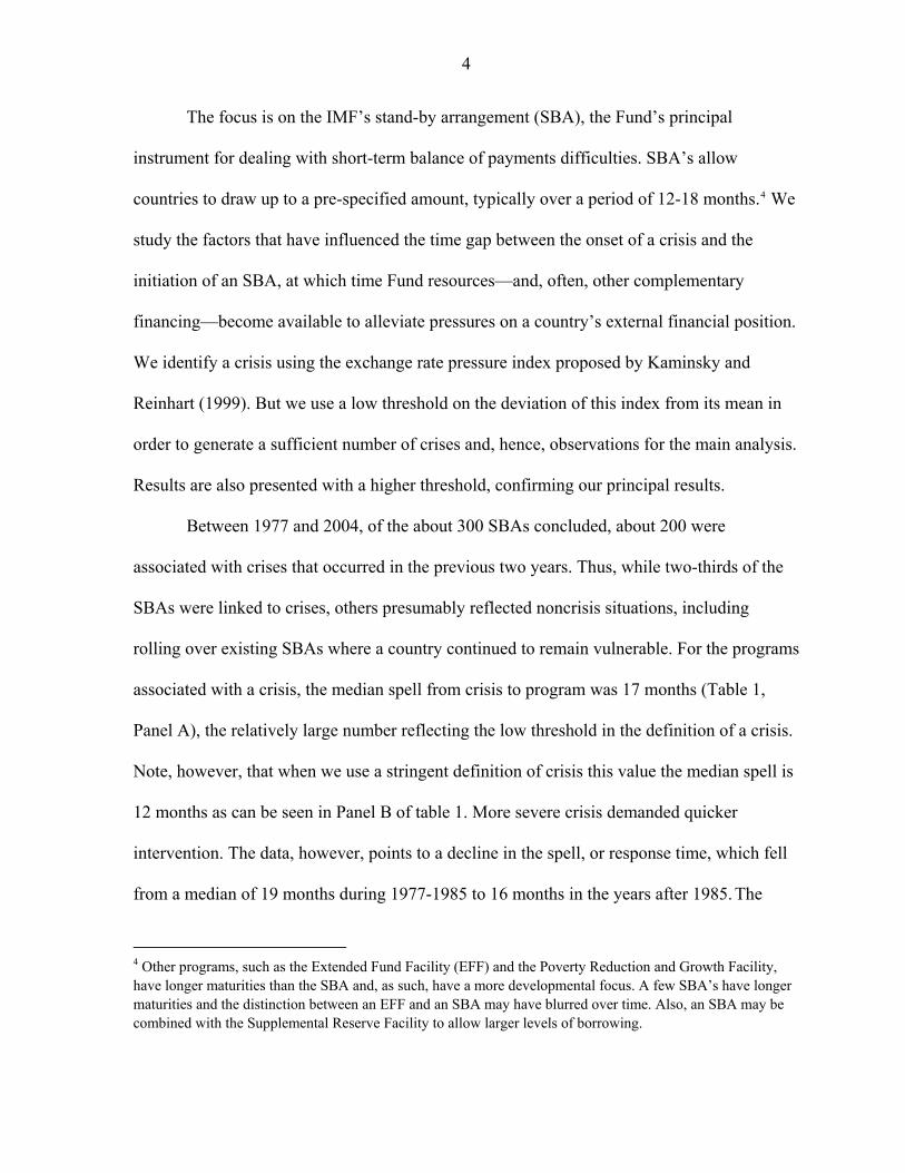
The focus is on the IMF’s stand-by arrangement (SBA), the Fund’s principal

instrument for dealing with short-term balance of payments difficulties. SBA’s allow

countries to draw up to a pre-specified amount, typically over a period of 12-18 months.4 We

study the factors that have influenced the time gap between the onset of a crisis and the

initiation of an SBA, at which time Fund resources—and, often, other complementary

financing—become available to alleviate pressures on a country’s external financial position.

We identify a crisis using the exchange rate pressure index proposed by Kaminsky and

Reinhart (1999). But we use a low threshold on the deviation of this index from its mean in

order to generate a sufficient number of crises and, hence, observations for the main analysis.

Results are also presented with a higher threshold, confirming our principal results.

Between 1977 and 2004, of the about 300 SBAs concluded, about 200 were

associated with crises that occurred in the previous two years. Thus, while two-thirds of the

SBAs were linked to crises, others presumably reflected noncrisis situations, including

rolling over existing SBAs where a country continued to remain vulnerable. For the programs

associated with a crisis, the median spell from crisis to program was 17 months (Table 1,

Panel A), the relatively large number reflecting the low threshold in the definition of a crisis.

Note, however, that when we use a stringent definition of crisis this value the median spell is

12 months as can be seen in Panel B of table 1. More severe crisis demanded quicker

intervention. The data, however, points to a decline in the spell, or response time, which fell

from a median of 19 months during 1977-1985 to 16 months in the years after 1985. The

4 Other programs, such as the Extended Fund Facility (EFF) and the Poverty Reduction and Growth Facility, have longer maturities than the SBA and, as such, have a more developmental focus. A few SBA’s have longer maturities and the distinction between an EFF and an SBA may have blurred over time. Also, an SBA may be combined with the Supplemental Reserve Facility to allow larger levels of borrowing.

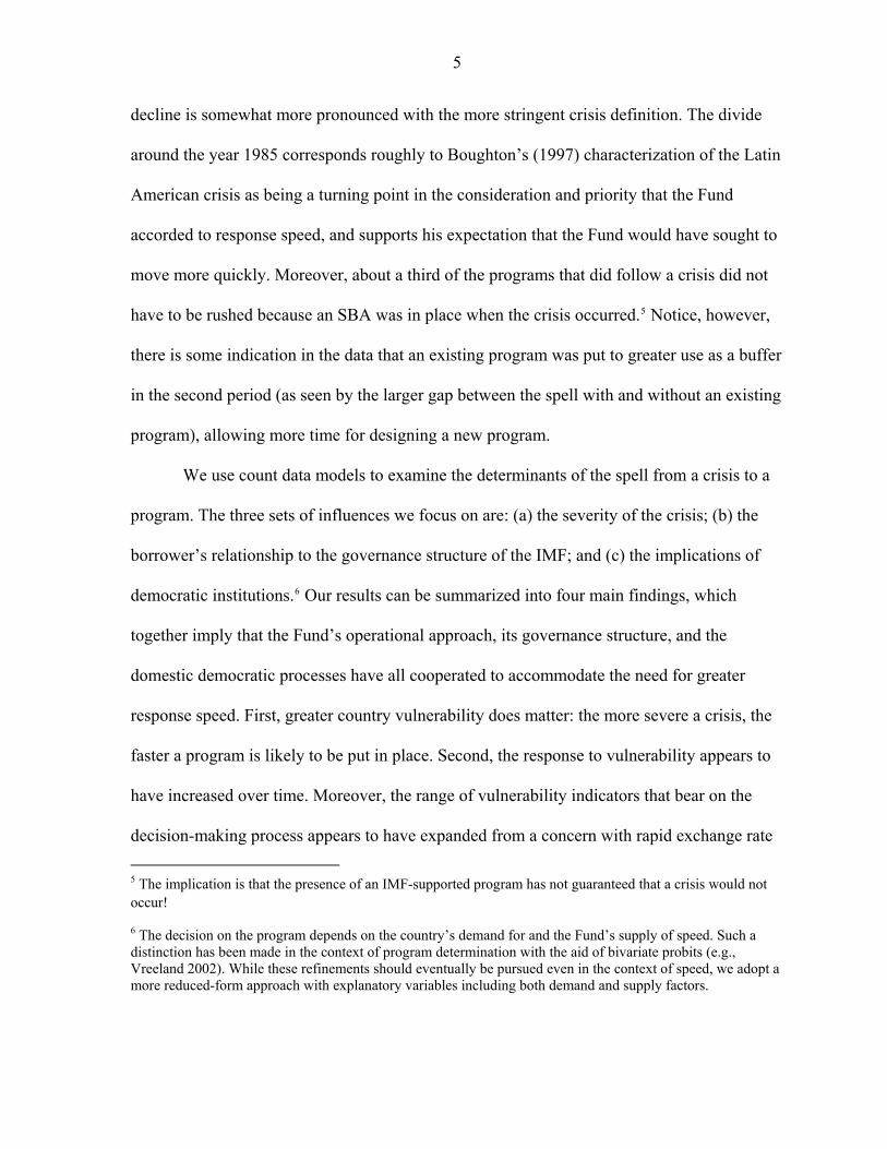
5

decline is somewhat more pronounced with the more stringent crisis definition. The divide

around the year 1985 corresponds roughly to Boughton’s (1997) characterization of the Latin

American crisis as being a turning point in the consideration and priority that the Fund

accorded to response speed, and supports his expectation that the Fund would have sought to

move more quickly. Moreover, about a third of the programs that did follow a crisis did not

have to be rushed because an SBA was in place when the crisis occurred.5 Notice, however,

there is some indication in the data that an existing program was put to greater use as a buffer

in the second period (as seen by the larger gap between the spell with and without an existing

program), allowing more time for designing a new program.

We use count data models to examine the determinants of the spell from a crisis to a

program. The three sets of influences we focus on are: (a) the severity of the crisis; (b) the

borrower’s relationship to the governance structure of the IMF; and (c) the implications of

democratic institutions.6 Our results can be summarized into four main findings, which

together imply that the Fund’s operational approach, its governance structure, and the

domestic democratic processes have all cooperated to accommodate the need for greater

response speed. First, greater country vulnerability does matter: the more severe a crisis, the

faster a program is likely to be put in place. Second, the response to vulnerability appears to

have increased over time. Moreover, the range of vulnerability indicators that bear on the

decision-making process appears to have expanded from a concern with rapid exchange rate

5 The implication is that the presence of an IMF-supported program has not guaranteed that a crisis would not occur!

6 The decision on the program depends on the country’s demand for and the Fund’s supply of speed. Such a distinction has been made in the context of program determination with the aid of bivariate probits (e.g., Vreeland 2002). While these refinements should eventually be pursued even in the context of speed, we adopt a more reduced-form approach with explanatory variables including both demand and supply factors.

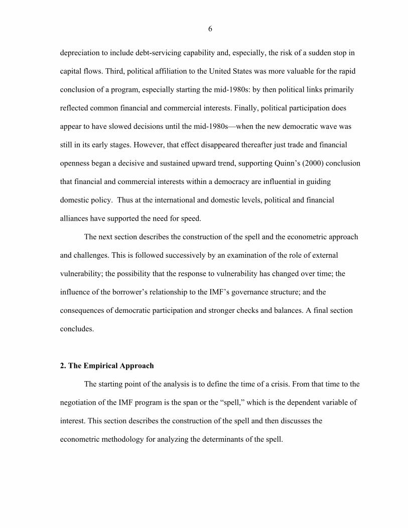
6

depreciation to include debt-servicing capability and, especially, the risk of a sudden stop in

capital flows. Third, political affiliation to the United States was more valuable for the rapid

conclusion of a program, especially starting the mid-1980s: by then political links primarily

reflected common financial and commercial interests. Finally, political participation does

appear to have slowed decisions until the mid-1980s—when the new democratic wave was

still in its early stages. However, that effect disappeared thereafter just trade and financial

openness began a decisive and sustained upward trend, supporting Quinn’s (2000) conclusion

that financial and commercial interests within a democracy are influential in guiding

domestic policy. Thus at the international and domestic levels, political and financial

alliances have supported the need for speed.

The next section describes the construction of the spell and the econometric approach

and challenges. This is followed successively by an examination of the role of external

vulnerability; the possibility that the response to vulnerability has changed over time; the

influence of the borrower’s relationship to the IMF’s governance structure; and the

consequences of democratic participation and stronger checks and balances. A final section

concludes.

2. The Empirical Approach

The starting point of the analysis is to define the time of a crisis. From that time to the

negotiation of the IMF program is the span or the “spell,” which is the dependent variable of

interest. This section describes the construction of the spell and then discusses the

econometric methodology for analyzing the determinants of the spell.

7

The spell: crisis and response

In defining a crisis, we were guided by the Kaminsky and Reinhart (1999) gauge of

the pressures faced by a country’s currency.7 These pressures can be captured by significant

variations in the exchange rate and foreign currency reserves. The larger the depreciation and

the loss of reserves, the greater is the pressure. Kaminsky and Reinhart propose a composite

indicator based on monthly changes in the exchange rate and reserves.

R

R

e

eI

R

e

“e” is the end-of-the-month exchange rate, “R” is the end-of-the-month reserves’ level, and

the Δ operator refers to monthly change.8 The rate of change of reserves is normalized by the

ratio of the standard deviation of exchange rate (σe) to the standard deviation of rate of

change of reserves (σr). In Kaminsky and Reinhart, a country is defined as entering a crisis in

the month when this indicator is three standard deviations off its mean for that country. Our

indicator is softer: it turns on when the index is one standard deviation above its mean. This

allows us to identify a larger number of events as “crises,” providing us with more data

points to analyze the duration from a crisis to a Fund program. We compensate for this by

allowing, in the regressions, for continuous variation in the severity of the crisis, as measured

by the extent of the depreciation and exchange rate loss.9 Kaminsky and Reinhart (1999)

show in their Figure 4 that a crisis evolves over time to reveal its severity. Thus, a slow drain 7 The focus on currency crises is determined by the practical difficulty of dating, for example, banking and debt crises.

8 Some also include the change in interest rate in this pressure index. However, the lack of comparable interest rate data across a broad range of countries typically limits this addition.

9 We also present results using a tighter crisis definition: a 1.5 standard deviation threshold: the number of observations drops considerably but the results remain qualitatively similar.

8

of reserves is followed initially by a sharp depreciation of the exchange rate. The “crisis”

month is typically the first in which a (generally overvalued) exchange rate makes a sizeable

move following the loss of reserves. Exchange rate depreciation then continues (while

reserves generally bottom out). Hence, the degree to which the exchange rate depreciation

persists and is subsequently followed by even more serious difficulties, such as a sudden stop

in capital flows determines how severe the crisis is. In our empirical analysis, we examine

the significance of this variation in crisis severity.

An observation enters our sample when an IMF stand-by arrangement (SBA) was

preceded by a crisis in the prior two years. We use the IMF’s “Date of Arrangement” as the

date on which the program came into effect. The span between the month of arrangement and

the month of the crisis gives us our dependent variable, the spell. Since we have no direct

way to link a crisis to a particular SBA, we assume that if a program was negotiated within

two years of the crisis, it was related to that particular crisis.10 Clearly, the two-year time

window within which we scanned was set arbitrarily. As with the definition of the crisis, it

was a compromise to generate a sufficient number of observations for analysis. In this way, it

was possible to relate around 200 SBA programs to our crisis indicator during the time span

January 1977 to December 2004. In practice, because the right-hand-side explanatory

variables were sometimes missing, we work with a sample of about 183 observations.

An alternative strategy—one that might be thought to be more natural and direct—

would be to identify all crises and then determine if and how long after the crisis an IMF

program followed. This would lead to the estimation of a hazard model. A key difficulty with

10 If there were multiple crises within the two-year period prior to the particular program, the first crisis was used to define the spell.

9

this approach in our context is that crises come in bunches. As such, it is often the case that a

crisis will follow one or more crises. In this case, it is unclear which crisis to associate with

the program—alternatively, we would have more than one spell associated to the same

program.11 Instead, the convention we adopt of using the earliest crisis in a two-year window

before a program implies that the first crisis, followed by other crisis events, triggered the

eventual program. To retain the information on the incidence of subsequent crises, we

include in the regressions dummy variables to reflect if a subsequent crisis occurred in the

first three months and the first six months following the original crisis.

As noted in the introduction, for the entire sample, the median time between crisis

and program initiation was 17 months. There was considerable variation in the spell, with the

25th percentile value of 9 months and the 75th percentile value of 22 months. Some programs

were rapidly negotiated, the 1995 Mexico SBA in 1 month and the 2002 Brazil and Uruguay

SBA’s in less than 2 months.

The presumption is that speed is necessary to prevent an economic slide in the

country hit by a crisis while also limiting contagion to other countries. For a first look at the

country’s circumstances, we examine the growth contraction in the year of the crisis and the

recovery in the three years thereafter. In line with Boughton’s periodization and our

subsequent analysis, we divide the sample period into two parts, 1977-1985 and 1986-2004.

Table 2 shows that growth shocks were greater in the first period, as seen in the larger

negative growth rates of per capita GDP in the year of the program. This was so whether a

program was in place or not. Following the shock, there is evidence of mean reversion in

11 This implies that we do not use censored observations in our regressions (i.e. a crisis not related to a program). Consequently, we are estimating the time span between a crisis and a program, conditional on a program being associated with a crisis.

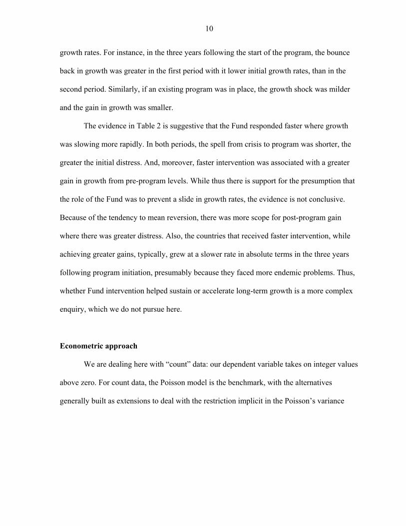
10

growth rates. For instance, in the three years following the start of the program, the bounce

back in growth was greater in the first period with it lower initial growth rates, than in the

second period. Similarly, if an existing program was in place, the growth shock was milder

and the gain in growth was smaller.

The evidence in Table 2 is suggestive that the Fund responded faster where growth

was slowing more rapidly. In both periods, the spell from crisis to program was shorter, the

greater the initial distress. And, moreover, faster intervention was associated with a greater

gain in growth from pre-program levels. While thus there is support for the presumption that

the role of the Fund was to prevent a slide in growth rates, the evidence is not conclusive.

Because of the tendency to mean reversion, there was more scope for post-program gain

where there was greater distress. Also, the countries that received faster intervention, while

achieving greater gains, typically, grew at a slower rate in absolute terms in the three years

following program initiation, presumably because they faced more endemic problems. Thus,

whether Fund intervention helped sustain or accelerate long-term growth is a more complex

enquiry, which we do not pursue here.

Econometric approach

We are dealing here with “count” data: our dependent variable takes on integer values

above zero. For count data, the Poisson model is the benchmark, with the alternatives

generally built as extensions to deal with the restriction implicit in the Poisson’s variance

11

structure.12 For a random variable, “y” that follows the Poisson distribution, the probability

that it takes the value “j” is given by13:

( )!

jeP y j

j

0, 0,1,2,...j

The parameter, λ, thus defines the distribution. In particular, the expected value and

the variance of y are equal to λ, i.e., ( )E y and var( )y . For economic applications, λ

is treated as a function of the variables of interest, represented by the vector x. As such, the

outcome for a particular observation “i”, “yi”—which, in our case, is the “spell” between the

crisis and program initiation—follows a Poisson distribution with the parameter ,

conditional on the vector of attributes “xi,” the observed influences,

i

( )i i iy Poisson x , where exp( )i i x

The econometric task is to estimate vector β, which contains the response parameters of

interest. Note, that larger values of the elements of β imply a larger spell and hence a slower

speed of response. Thus, for any observation “i,” conditional on observing the vector of

attributes “xi,” the probability of observing an outcome “yi” is given by:

exp( exp( )) exp( )( X )

!

iyi i

i i i ii

P Y yy

x xx 0,1, 2,...iy

12 Poisson estimation can be interpreted as a duration model with a constant hazard rate.

13 The presentation and notation here follows Winkelmann and Boes (2006). Early development of count data models was presented by Hausman, Hall, and Griliches (1984). A widely used text book treatment is Cameron and Trivedi (1998).

12

This probability function forms the basis for defining the likelihood function over the set of

observations, and the parameters are estimates are obtained by maximizing the function. The

expected value and the variance now are:

( ) exp( )i i iE y x x var( ) exp( )i i iy x x

Notice that as the expected value increases, so does the variance, implying heteroscedasticity.

However, a concern is that the variance may, in fact, rise even faster. If present, this

“unobserved heterogeneity,” would underestimate the variance and, hence, the standard

errors of the estimates. Thus, if the true Poisson parameter is i and i represents the

unobserved heterogeneity, then, i is related to the observed i as follows:

exp( )i i i x

exp( ) exp( ) exp( )i i i i iu ui i x x

i

exp( )i u , and it is assumed without loss of generality that ( )i iE u x 1

and 2var( )i i iu x . It follows that the expected value of i is i , which implies that the

Poisson parameter estimates are not biased. However, the Poisson model underestimates the

variance, which now is:

2 2var( )i i i i iy x

The problem is referred to as one of “over dispersion.” A commonly used solution is the

Negative Binomial model, which is based on the further assumption that has a gamma

distribution with parameter

iu

. Further, if:

13

21 i

ii

, 2var( ) (1 ) exp( )i i i iy x x .

A more complex likelihood function ensues, which can be found in standard

references such as Cameron and Trivedi (1998) or Winkelmann and Boes (2006). But while

it is expedient to employ a Negative Binomial model to allow for additional heterogeneity,

there are costs to doing so. The model specifies a very specific error structure of the

unobserved (and, hence, omitted) variables, with a very specific distribution. In practice, it

remains important to search for these unobserved variables directly. Thus, in their seminal

contribution, Hausman et al. (1984) point out that addition of plausible explanatory variables

is an important first step, which should have the effect of reducing the unobserved

component of the heterogeneity. In their application, they note, for example, that allowing for

time variation in the effectiveness of R&D in generating patents reduces such heterogeneity

and hence provides for a better empirical specification. As they also note, the same purpose

is served by fixed effects—in our case, country and time fixed effects. The country fixed

effects imply that unchanging but unobserved country-specific factors influence the spell;

and the time fixed effects allow for unobserved effects in different years, e.g., threat of

financial contagion across countries.

But there remain limits to adding explanatory variables. One solution lies then in

correcting for standard errors. As Winkelmann and Boes (2006, p. 289) point out, “there are

many possible reasons, apart from unobserved heterogeneity, why the conditional variance in

the Poisson model would depart from the conditional mean.” The departure has

consequences similar to those arising from heteroscedasticity in linear regression models:

“the parameter estimates remain consistent, but the usual variance matrix is inconsistent and

the estimator is inefficient.” They recommend using the Poisson model with robust standard

14

errors. They caution, moreover, that a mechanical resort to alternative estimators is risky

since the alternatives may fail even in generating consistent estimates if the underlying

assumptions are violated. Such would be the case for a Negative Binomial model if the

unobserved heterogeneity was not gamma distributed.

The procedure we follow, therefore, is to gradually build up the Poisson model by

adding explanatory variables and, in particular, allowing for time variation in response.

Throughout we include country and time dummies and report robust standard errors clustered

on the country. Use of country dummies is possible since virtually all countries in the sample

have multiple programs, allowing control for unchanging country-specific features that may

condition the negotiation with the IMF. We provide comparisons with the Negative Binomial

model and show that the fully-specified Poisson and Negative Binomial models have

virtually-indistinguishable results.14

3. Economic Vulnerability and Speed of Response

While preserving international stability requires acting expeditiously, program design

may imply proceeding more cautiously. In responding to financial crises, does the IMF

accord priority to speed of response necessary for stemming a country’s external

vulnerability or is the focus, instead, on the time needed to design complex reforms to

reverse the conditions that led to the crisis? If a country facing a crisis is a victim of events

14 The Negative Binomial model also includes country and time dummies, as recommended by Allison and Waterman (2002). These authors point out that the “fixed-effects” Negative Binomial model proposed by Hausman et al. (1984) is not a true fixed-effects model and suggest including fixed effects directly, advice we have followed. Also, the Poisson model can be interpreted as a duration model with a constant hazard rate. For robustness check, we ran duration models with different assumptions about the hazard rates and results are qualitatively similar. These estimations are not reported in the paper but they are available upon request.

15

beyond its control, speed is unequivocally of the essence. But typically the crisis reflects the

accumulation of imbalances from policy errors. Reversing policy is needed to set the country

on a more sustainable path and, in doing so, to safeguard the Fund’s resources being loaned

to the country. Balancing the need for speed with protecting its resources has been a

continuing challenge for the Fund. The operational question is whether the policy

conditionality accompanying a Fund-supported program can be agreed on rapidly. While

some programs (including with deep, possibly intrusive, conditionality) have been put

together quickly, the presumption is that this will generally not be the case.

Throughout, the regressions control for the presence of a pre-existing IMF program at

the time of the crisis and for the incidence of additional crises in the first and second quarters

after the first one in the time window of two years before the program. As expected, and as

reported in Table 3, if a program is already in place, all else equal, the existing program

appears to provide an umbrella for Fund assistance and hence reduces the urgency for a new

program.15 Also, the coefficient on the dummy variable that indicates the presence of a crisis

in the first quarter following the original crisis is almost never significant. The variable that

indicates the presence of a crisis in the second quarter after the original crisis is positive but

losses significance in the regressions where we split the period of analysis. The positive sign

suggests that the IMF takes more time to assist a country in more unstable situations.

With those controls in place, this section explores how the severity of the crisis

influences the speed of response. To that end, we employ several measures to assess the

country’s vulnerability, with a focus on the country’s balance of payments position. First, in

15 The Fund can modify the existing program to accommodate the new post-crisis situation, through a new “letter of intent” and fresh disbursement

16

line with Kaminsky and Reinhart (1999), and as noted above, we consider a crisis more

severe the larger is the loss of reserves (in the six months before the date of the crisis) and the

greater is the exchange rate depreciation (in the six months after the date of the crisis).16 The

results are as expected. A larger depreciation and a larger loss of reserves are, in fact,

associated with a faster response speed (a smaller spell). The level of statistical significance

does vary across specifications. In this full sample, exchange rate depreciation is always

significant at the conventional 5 percent level but reserve loss is significant only at around

the 10 percent significance level.

The influence of global conditions at the time of the crisis is less clear. A tight U.S.

monetary policy, reflected in a higher U.S. Federal Funds rate, is associated with restricted

emerging market access to international capital (Calvo, Leiderman, and Reinhart, 1996).

However, we find that a higher Federal Funds rate is actually associated with a slower

program conclusion (Columns 1 and 4). Petroleum prices do not have a significant effect.

There appears to be some collinearity between the Federal Funds rate and petroleum prices.

Also, both variables have offsetting effects. A higher interest rate increases the costs of

borrowing but also increases returns on reserves and other liquid assets. Higher petroleum

prices damage some current accounts (requiring external assistance) but they also increase

surpluses in oil-rich countries and recycling of these surpluses eases conditions in global

capital markets and hence reduce the pressure to respond speedily (see also Gupta,

16 We considered somewhat different time spans, but with qualitatively similar results.

17

Eichengreen, and Mody 2008). The possibility that these two effects of petroleum price have

changed in relative strength over time is pursued below.17

Next, in Table 4, we consider a variety of measures in the year the program was

initiated. Where the spell is short, they also reflect conditions close to the crisis; for longer

spells, they capture the evolution following the crisis and the conditions closer to the decision

on the IMF program. Rapid exchange rate depreciation remains a reason to speed program

initiation. Reserve loss maintains its sign, but is now not significant. Instead, the loss of

reserves is subsumed by a sudden stop in capital flows, which is a call to action and produces

a quick response. This is consistent with the Fund’s mandate to stem the after-shocks from

developments in international capital markets. A more rapid growth rate, not surprisingly,

slows down program speed, as the descriptive statistics in Table 2 had suggested. Inclusion

of growth rate reduces somewhat the strength of the sudden stop variable—again, not

surprising since sudden stops are correlated with slower growth. Finally, the debt service-to-

exports ratio and the occurrence of a systemic banking crisis apparently do not, on average,

speed up an IMF program.

While these results are suggestive, the test diagnostics for the Poisson regressions in

Table 4 suggest that “over dispersion” (variance of the Poisson parameter greater than its

mean) cannot be rejected. As discussed above, robust standard errors help correct for the

possibility that the standard errors are underestimated and the fact that the Negative Binomial

regression gives similar results indicates that there is merit to the basic specification

17 It is also likely that petroleum price will influence countries differently, depending, for example, on whether they are oil importers or exporters. However, inclusion of country dummies implies that controlling for country characteristics an increase over time in the prevailing petroleum price at successive crises reduced the urgency of a needed response from the IMF.

18

employed. But it is not precise enough. In the spirit, therefore, of Hausman et al. (1984), a

question of interest is whether the unobserved heterogeneity reflects changes over time in the

responsiveness to the triggers that lead to initiation of IMF programs. In other words, has

there been a change in how quickly a Fund program is established for a given exchange rate

depreciation? Has the demand for speed increased with more encompassing financial

globalization? The answer appears to be a clear “yes.”

4. Changes over Time

The debt crises of the 1980s highlighted the need for speed in responding to crises,

reflecting the increasing vulnerability to rapid capital outflows. By Boughton’s (1997, p.3)

assessment, prior to the international debt crisis of 1982, “... the Fund had helped countries

through numerous crises, but its role in those cases was essentially similar to its noncrisis

lending activities.” However, “... when the 1982 crisis erupted, the Fund’s response quickly

broadened into a more systemic function.” In particular, one country’s challenge to service

its debt placed other countries at risk since lenders’ balance sheets were weakened and/or

lenders perceived risks as correlated across countries. These lessons, he concludes, were

learnt gradually but came to be incorporated in the Fund’s operational approach by the

second half of the 1980s, as the Fund increasingly viewed itself as a “crisis manager.”

Bordo and James (2000, p. 32-33) also draw attention to the pressures to act quickly.

They point to the growing reliance of emerging market governments and businesses on

borrowing from dispersed lenders through international capital markets. Already, according

to Boughton, Mexico’s default on bank debt in 1982 had raised spillover and systemic

19

concerns and alerted the Fund on the need for speed. The next big test was Mexico’s

“tesobono” crisis of 1994-1995. The significant shift towards capital markets implied that:

“...much more rapid action was required, and also a greater commitment of funds, because the number of actors was so much greater. It was impossible to use the strategy of 1982, and corral the foreign investors (who were now not banks, but instead were represented in innumerable mutual and pension funds). There was a fear of a global contagion, and a belief that the only way to limit such contagion lay in the extension of some protection to investors.” The trend has been relentless. With financial markets larger and more integrated,

small shifts in sentiment can severely hurt not only the country directly affected but can,

through various channels of contagion, draw other countries, including so-called “innocent

bystanders,” into the financial turbulence. To limit this damage, speed is an important

element of the policy response.

To explore these considerations we divide the sample in two parts following the

above discussion: 1977-1985 and 1986-2004. The first period captures the second oil shock

(in 1979) and its aftermath; it is also the period of rapid build up of international debt,

followed by the debt crisis, centered on Latin America. Unable to repay debt used to finance

large current account deficits, several countries had to restructure their external debt, were

cut off temporarily from sources of external credit, and experienced negative growth

(Edwards 1995 and Table 2 above). The crisis, as Boughton has emphasized, was a turning

point in the Fund’s recognition of the need for speed. In the second period, the consolidation

following the Latin American debt crisis initially implied a withdrawal of foreign capital

flows from emerging markets but then witnessed a renewed inflow of international capital

that culminated in “irrationally exuberant” lending and the string of emerging market crises.

Since the two time periods cannot be dated exactly, we present some alternatives below.

20

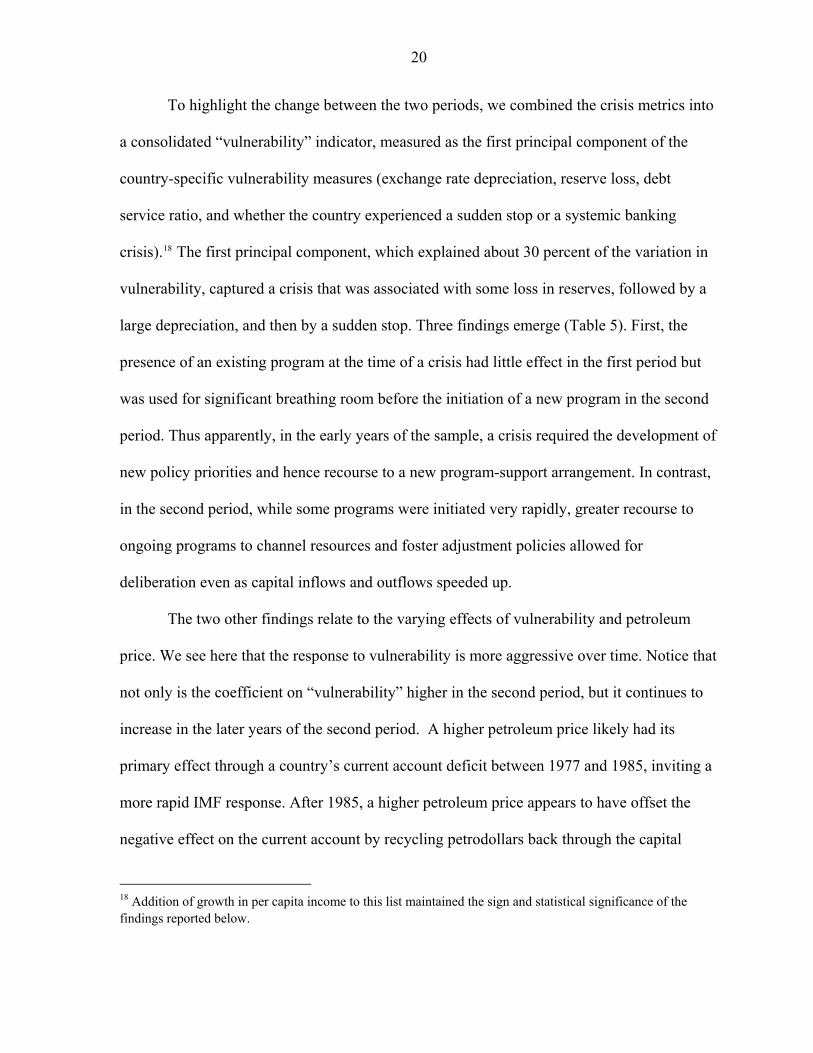
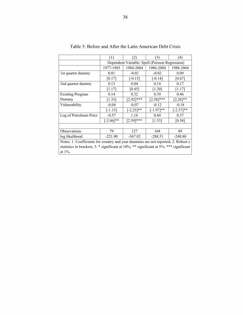
To highlight the change between the two periods, we combined the crisis metrics into

a consolidated “vulnerability” indicator, measured as the first principal component of the

country-specific vulnerability measures (exchange rate depreciation, reserve loss, debt

service ratio, and whether the country experienced a sudden stop or a systemic banking

crisis).18 The first principal component, which explained about 30 percent of the variation in

vulnerability, captured a crisis that was associated with some loss in reserves, followed by a

large depreciation, and then by a sudden stop. Three findings emerge (Table 5). First, the

presence of an existing program at the time of a crisis had little effect in the first period but

was used for significant breathing room before the initiation of a new program in the second

period. Thus apparently, in the early years of the sample, a crisis required the development of

new policy priorities and hence recourse to a new program-support arrangement. In contrast,

in the second period, while some programs were initiated very rapidly, greater recourse to

ongoing programs to channel resources and foster adjustment policies allowed for

deliberation even as capital inflows and outflows speeded up.

The two other findings relate to the varying effects of vulnerability and petroleum

price. We see here that the response to vulnerability is more aggressive over time. Notice that

not only is the coefficient on “vulnerability” higher in the second period, but it continues to

increase in the later years of the second period. A higher petroleum price likely had its

primary effect through a country’s current account deficit between 1977 and 1985, inviting a

more rapid IMF response. After 1985, a higher petroleum price appears to have offset the

negative effect on the current account by recycling petrodollars back through the capital

18 Addition of growth in per capita income to this list maintained the sign and statistical significance of the findings reported below.

21

account, reducing the urgency of response. The implication is that while larger capital

flows—and their easy reversibility, creating sudden stops—posed more of a threat in the

second period, the size of the international capital markets also provided financial recourse to

supplement IMF resources.

The test statistics are encouraging. The hypothesis of over dispersion is rejected for

the first period and the second period, if that is thought to have started from 1988. The

second period, either from 1984 or 1986 still tends to indicate the presence of unobserved

heterogeneity, implying further search for omitted variables.

4. The Borrower’s Relationship with the Fund

A feature of IMF governance, emphasized by Barro and Lee (2005), is the share of a

country’s quota in the aggregate “subscriptions” (funding) from all member countries.19

Barro and Lee find that a larger quota share raises the likelihood of a Fund program. Other

research, however, is less supportive of this conclusion (see, for example, Eichengreen,

Gupta, and Mody 2008). Countries with larger quota shares may have somewhat greater

clout but they may also be more reluctant to draw on the Fund for reputational reasons.

Moreover, as the British example following the Suez crisis shows, a significant quota may

yet prove insufficient. Boughton (2001) notes that the British, facing a run on the sterling in

the aftermath of the 1956 Suez crisis, looked to the “apolitical” support of the IMF to draw

on the large amounts to which they were “virtually entitled” as one of the two major

19 “Quota subscriptions generate most of the IMF's financial resources. Each member country of the IMF is assigned a quota, based broadly on its relative size in the world economy. A member’s quota determines its maximum financial commitment to the IMF, its voting power, and has a bearing on its access to IMF financing.” http://www.imf.org/external/np/exr/facts/quotas.htm.

22

founding countries and the second-largest member. But success in doing so hinged on

garnering U.S. backing through compliance with the U.S.-supported United Nations’

resolution to resolve the political crisis.

A growing number of statistical studies have concluded that political and economic

affinity with the major IMF shareholders places a country in a stronger position to obtain

IMF support. Thacker (1999) first showed that countries that have tended to vote with the

United States in the United Nations were also more likely to receive IMF program support.

Barro and Lee (2005) found that UN voting concordance and larger trade shares with the

United States were associated with stronger probabilities of obtaining IMF lending as well as

with a larger size of lending.20 The mechanism behind this result is in the Broz and Hawes

(2006) finding that private financial lobbies influence U.S. Congressional votes in favor of

IMF quota increases. Along with Oatley and Yackee (2004), they also report that, all else

equal, the likelihood of lending and the amount of IMF lending is higher the greater is the

exposure of U.S. money center banks in the borrowing countries.

Our results are reported in Table 6.21 We revert here to identifying the specific

vulnerability variables to examine their roles separately rather than in a composite indicator.

We present results for the two periods, with the full set of variables used so far and then

pared down to allow for multicollinearity. Column (2) is a more parsimonious version of

column (1) for the first period (i.e., before 1986). In that period, it appears that the two

sources of vulnerability were a country’s currency depreciation and a rise in the petroleum

20 Unlike in other studies, Barro and Lee (2005) also found similar effects vis-à-vis European shareholders.

21 A broader set of Fund incentives and capabilities for response could be considered but metrics for these are not easy to define. Similarly, of Fund conditionality and its intrusiveness could impact response speed. Once again, persuasively measures of conditionality (beyond just the number of conditions) are required.

23

price. This lends some plausibility to a view that most crises during this period had their

origins primarily in current account imbalances.22 Neither IMF governance variable is

statistically significant—closer affiliation with the U.S., if anything, slows down Fund

programs in that early period. In column (3), we add the country’s per capita GDP (in PPP

terms). This addition is another effort to control for institutional and other omitted variables.

The results reported remain unchanged but we do find in the first period that countries with

higher per capita incomes were prone to more speedily conclude negotiations. Presumably,

stronger institutions helped.

For the second period, starting in 1986, the results are different in important respects

(columns 4 and 5). The exchange rate depreciation variable turns statistically insignificant

but a broader range of vulnerability indices appear to have exercised influence. The

occurrence of a sudden stop was particularly potent. Loss of reserves and higher debt-service

to export ratio also elicited a faster response, although their statistical significance is reduced

when the country’s per capita income and growth rate are also included in the regression,

suggesting multicollinearity. Also, as reported above, the existing program dummy is

positive and significant, reaffirming the use in the second period of existing programs to

provide support when a new crisis emerged. The petroleum price variable turns positive as

before, but with varying significance levels.

The IMF quota share is, as in the first period, negative but insignificant. There is,

however, some evidence that closer affinity to the U.S. appears associated with faster

program negotiation. It is as if during this latter period the broader sources of vulnerability in

22 Their manifestation as debt crises with collateral implications for international banks and, hence, for possible contagion, raised the broader issues of the need for speed.

24

the context of faster moving capital markets increased the value of speed and induced

countries to use their political links to ensure timely decisions in the context of higher risks

from delays. This result echoes Thacker’s (1999) and Oatley and Yackee’s (2004) findings.

They report that the relevance of affinity with the U.S. in securing access to IMF lending

increased sharply in the late 1980s. We find that same trend for the speed of response.

Thacker (1999) notes but leaves unresolved the reason for this shift. The conclusion of the

Cold War may have led some to expect that the U.S. interest in political alliances would

diminish over time. While we do not pursue this question in any great depth, results in the

next section suggest that economic interests became a more salient basis for political

alliances, in line with Oatley and Yackee (2004) and Broz and Hawkes (2006).

With the addition of the governance variables in Table 6, even the results for the

1986-2004 period show no evidence of over dispersion. A longer “second period” starting in

1984 fails the over dispersion test and shows considerable differences in results from that

starting in 1986. In particular, the value of political affiliation to the United States kicks in

after 1988. Clearly, these are not formal tests given our short time periods and, as such, our

assumption of the timing of the break in 1985 should be treated as indicative.

5. Has Globalization Curtailed Deliberative Democracy?

Democracies are thought to be inherently slow because they are based on the

obligation to encourage consensus. It could be that more deeply-rooted, deliberative

democracies—with more voices included in achieving a policy consensus—slow down the

negotiations in agreeing on IMF programs. If so, this conflicts with the needs of fast-moving

financial markets, and these needs may trump deliberation. Quinn (2000), however, argues

25

that there may be no conflict. In his view, the interests supporting political participation and

economic openness are aligned because each views the other as reinforcement. As such, the

curtailment of deliberation may be a conscious choice backed by institutions that permit

rapid decisions.

The question we ask is whether democracies had an effect on the speed of concluding

an IMF program. Of course, empirical implementation is not straightforward. Democracies

come in many varieties. And the variations, which imply differing degrees of voice and

accountability, have significant implications for economic decisions. 23 The conventional

measure of political participation in democratic processes is the Polity IV measure. This

measure ranges for -10 representing the most autocratic regime to +10 for the most

democratic. As others have done (see Quinn 2000 and also the Polity IV webpage24), we

divide regimes into three categories. Observations with values of -5 to +5 are the base group

(with the democracy indicator taking the value zero): those with higher values are democratic

(and the indicator variable takes the value 1) and those with lower values are autocracies

(with the indicator variable defined as -1).25 In addition, for our purpose, Henisz’s (2002)

measure of veto points is particularly attractive. To contain the possibility of arbitrary

decision making, democratic institutions may introduce checks and balances. The PolConIII

indicator, which we use here, measures the extent to which the legislature can constrain the

23 While we have chosen to focus on democratic institutions as conditioning country incentives and capability for responding to crises, a variety of other political factors could, in principle, be influential. We leave that exploration for further research.

24 http://www.systemicpeace.org/polity/polity4.htm

25 In practice, various authors choose different cut off points. Our key results do not appear sensitive to the exact definition.

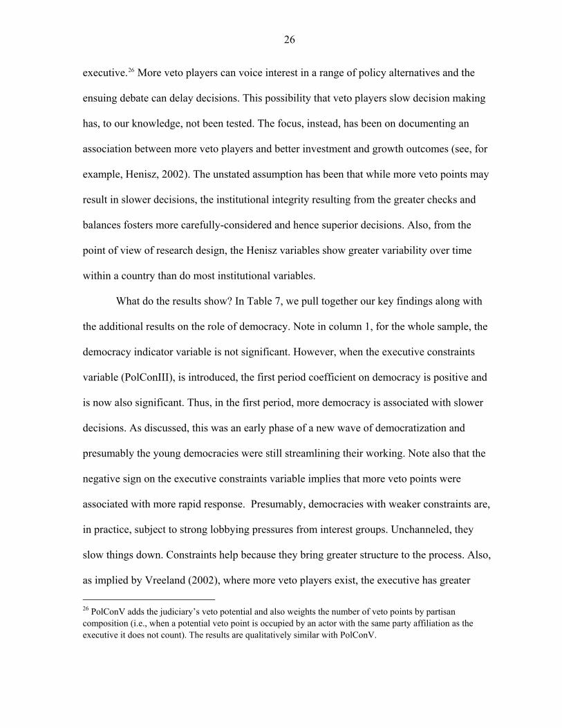
26

executive.26 More veto players can voice interest in a range of policy alternatives and the

ensuing debate can delay decisions. This possibility that veto players slow decision making

has, to our knowledge, not been tested. The focus, instead, has been on documenting an

association between more veto players and better investment and growth outcomes (see, for

example, Henisz, 2002). The unstated assumption has been that while more veto points may

result in slower decisions, the institutional integrity resulting from the greater checks and

balances fosters more carefully-considered and hence superior decisions. Also, from the

point of view of research design, the Henisz variables show greater variability over time

within a country than do most institutional variables.

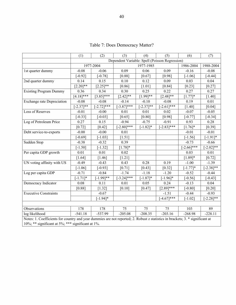
What do the results show? In Table 7, we pull together our key findings along with

the additional results on the role of democracy. Note in column 1, for the whole sample, the

democracy indicator variable is not significant. However, when the executive constraints

variable (PolConIII), is introduced, the first period coefficient on democracy is positive and

is now also significant. Thus, in the first period, more democracy is associated with slower

decisions. As discussed, this was an early phase of a new wave of democratization and

presumably the young democracies were still streamlining their working. Note also that the

negative sign on the executive constraints variable implies that more veto points were

associated with more rapid response. Presumably, democracies with weaker constraints are,

in practice, subject to strong lobbying pressures from interest groups. Unchanneled, they

slow things down. Constraints help because they bring greater structure to the process. Also,

as implied by Vreeland (2002), where more veto players exist, the executive has greater

26 PolConV adds the judiciary’s veto potential and also weights the number of veto points by partisan composition (i.e., when a potential veto point is occupied by an actor with the same party affiliation as the executive it does not count). The results are qualitatively similar with PolConV.

27

incentive to seek external support. In a crisis that incentive is exercised. Of course, the

Heinsz constraints variable may mainly be a measure of broader institutional quality

(carrying information that complements that in a country’s per capita income). The

accompanying policy credibility permits more rapid program negotiation. Thus democracies

have (at least two) divergent tendencies: political participation can slow things down but

institutions that curtail arbitrary decisions also create vents for quick decisions.

In the second period, the democracy variable is never significant. It could be that the

“wave” of democracy that emerged in the mid-1970s was still in its early stages during our

first period, 1977-1985, and that political participation had not matured in many of the new

democracies. Participants learned over time. The results for the second period continue to

show that the political constraints variable has a negative sign, but the magnitude of the

coefficient and its significance decline. This is especially so if the second period is

considered to start in 1986.

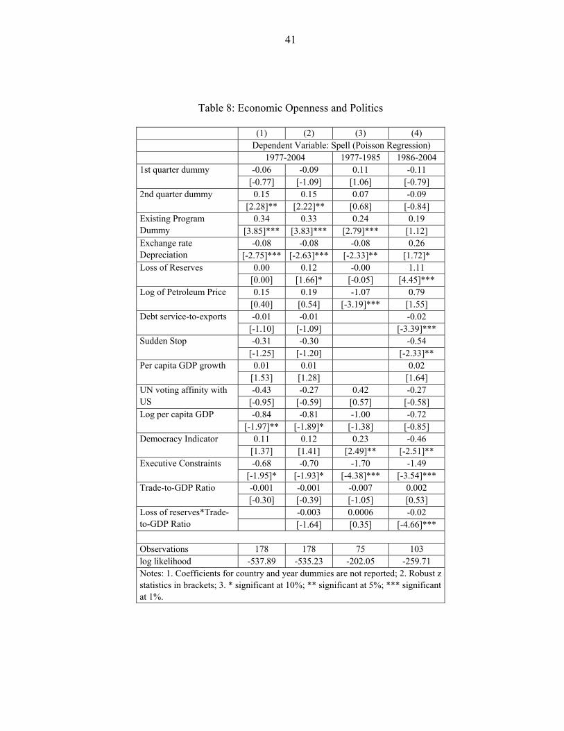
Consideration of a country’s economic openness further sharpens the results,

highlighting, in particular, the joint influences of economic and political openness. One

constraint on this analysis is the limited data on capital account openness, especially, but not

only, for the first period. However, a measure of trade openness, the sum of exports and

imports normalized by GDP, is available. The results we report here with trade openness are

largely corroborated by the smaller samples using the Chinn-Ito measure of capital account

openness, mirroring at the country level the aggregate trends in Figure 1.

With those preliminaries, the results in Table 8 show that openness by itself does not

influence speed. In the second period, however, the loss of reserves leads to more prompt

28

action, the more open the economy is.27 Thus, the effective response to loss of reserves (from

column 4 of Table 8) is 1.11 - 0.02*Trade/GDP. This is plotted in Figure 2(a) along with a 5

percent confidence interval band. For lower levels of trade-to-GDP, reserve loss is actually

associated with slower response and for the lowest 10 percent of the observations of the

trade-to-GDP ratio, the effective coefficient is marginally significant. However, as the trade-

to-GDP ratio increases, particularly beyond 56 percent, reserve losses begin to be viewed

with greater concern, leading to more rapid program conclusion. Notice in Figure 2(b) that

the trade-to-GDP ratio itself is never significant.

Figure 2(a): Effective Coefficient on Figure 2(b): Effective Coefficient on Reserve Loss Trade/GDP

-1.5

-1-.

50

.51

Effe

ctiv

e C

oef

ficie

nt o

f Re

serv

e L

oss

20 40 60 80 100

Trade/GDP (percent)

Effective Coefficient of Reserve Loss Lower BoundUpper Bound

-.02

-.01

0.0

1.0

2

Effe

ctiv

e C

oef

ficie

nt o

f Tra

de/G

DP

-1 -.5 0 .5

Reserve Loss

Effective Coefficient of Trade/GDP Lower BoundUpper Bound

Two by products of this exercise suggest interactions between economic openness

and politics. First, the executive constraints variable is now significant even in the second

period starting 1986 and with a point estimate that is much closer to that in the first period.

The inference is that some open countries experiencing loss of reserves had low executive

constraints. Once that influence is controlled for, the value of executive constraints is clearer

27 Other measures of crisis severity did not generate interesting results.

29

even in the second period. Second, the U.S. affinity variable reduces in significance in the

second period. This is the consequence of much greater correlation between trade openness

and the U.S. affinity variable in the second period (relative to the first). Thus, there is some

basis to the possibility that over time, in an increasingly integrated world economy, U.S.

political alliances are being driven by mutual commercial interests.

Finally, in Table 9, we reproduce Table 8 but using a tighter definition of crises.

Instead of a one standard deviation metric for the exchange rate pressure index, we report

results with 1.5 standard deviations. The results are interesting. With the tighter definition,

the variables that measure the intensity of the crisis become insignificant. This is not

surprising because crises in this sample are already more serious by definition—and the

results suggest that once this threshold is crossed, further variations in particular dimensions

of the crisis do not contribute to the speed of response. In contrast, the other variables retain

their sign and significance. Thus, our claim that politics—both international and domestic—

supports the need for speed continues to be validated.

6. Conclusions

This paper has made a first effort at mapping the Fund’s response speed and

examining its determinants. One of our conclusions is that the Fund’s approach to speed has

shifted in important ways since the mid-1980s as the pace of financial globalization has

increased. The relevance of financial integration is further supported by the finding that the

more open the economy the faster it responded to reserve losses in the second period. But the

data are limited and identifying these shifts is no easy matter. The results, although consistent

30

with the Fund’s increasing assumption of a crisis manager’s role in integrating global

economy, should be regarded as a benchmark for review and further analysis.

The common theme for the entire period of our study, from 1977 to 2004 is that the

Fund has responded faster when the threat of an economic slide has been greater. From 1977-

1985, crises took the form of current account distress, accompanied by large growth shocks.

More severe varieties of these crises motivated the Fund to move faster, but the pressure to

do so was less than after about 1985. The Latin American debt crisis, instigated by the

Mexican default in 1982, created greater awareness of international spillovers and systemic

risks. As international capital markets became more prominent, new facets of vulnerability

were revealed. The threat of a sudden stop, in particular, drew quick Fund attention as did

debt service obligations and reserve losses (for more open economies) in determining the

response speed. Recognizing the salience of these factors was, apparently, necessary to

contain the spread of the crisis with a view to maintaining international financial stability.

We did not pursue the difficult question of whether the Fund’s intervention helped raise the

country’s growth rate: that was not the intent of the intervention, in any case. Rather, growth

appears to have recovered, more so the greater the initial shock. While this may have mainly

reflected mean reversion, the finding does speak to the ongoing operational discussion on

design of rapid access Fund facilities. Prima facie quick and predictable delivery of support

necessary can help roll back a crisis while safeguarding the Fund’s financial position.

In line with case studies and statistical analyses, the role of the United States has

appeared as an important one. The results suggest that the U.S. has facilitated rapid decisions

and that this role has increased over time. The evidence in this paper also suggests that this

31

greater U.S. role has been associated with a shift from the Cold War period to greater interest

in economic alliances in an ever more integrated global market place.

Finally, with the onset of a new wave of global democratization in the mid-1970s,

political participation apparently hindered rapid response. But from the mid-1980s, political

participation appears to have evolved at least to the extent that it no longer slowed response

speed. A positive interpretation of this finding is that domestic democracy adapted to the

needs of these new generation crises. If true, the outcome is good for democracy and for the

future of financial globalization. But the finding is also consistent with better functioning

financial and commercial interests that are able to press for speed at times of crises.

32

References

Allison, Paul D. and Waterman, Richard P., 2002, “Fixed-Effects Negative Binomial Regression Models,” Sociological Methodology, 32, pp. 247-265.

Barro, Robert and Jong-Wha Lee, 200t, “IMF Programs: Who Is Chosen and What Are the

Effects,” Journal of Monetary Economics 52(7) 2005, pp. 1245-1269. Bird, Graham, 1996, “Borrowing from the IMF: the Policy Implications of Recent Empirical

Research,” World Development 24, pp. 1753-60. Bordo, Michael and Harold James, 2000, “The International Monetary Fund: Its Present Role

in Historical Perspective,” NBER Working Paper No. W7724. Boughton, James M., 1997, From Suez to Tequila: The IMF as Crisis Manager, IMF

Working Paper WP/97/90. A shorter version was subsequently published in The Economic Journal, 110 (460), pp. 273-291, 2000.

Boughton, James M., 2001, “Was Suez in 1956 the First Financial Crisis of the Twenty-First

Century?” Finance and Development 38 (3). http://www.imf.org/external/pubs/ft/fandd/2001/09/boughton.htm

Broz, J. Lawrence and Michael Brewster Hawes, 2006, “Congressional Politics of Financing

the International Monetary Fund,” International Organization 60 (Spring), pp. 367–399.

Calvo, G., L. Leiderman, and C. Reinhart, 1996, “Capital Flows to developing Countries in

the 1990s: Causes and Effects,” Journal of Economic Perspectives 10 (Spring), pp. 123-139.

Cameron, A.C. and P.K. Trivedi, 1998, Regression Analysis of Count Data, New York:

Cambridge University Press. Edwards, Sebastian, 1995, Crisis and Reform in Latin America: From Despair to Hope,

Washington D.C.: The World Bank. Eichengreen, B. and A. Mody, 1998, “Interest Rates in the North and Capital Flows to the

South: Is There a Missing Link?” International Finance 1, pp.35-58. Eichengreen, B., P. Gupta, and A. Mody, 2008, “Sudden Stops and IMF-Supported

Programs,” in Sebastian Edwards and Márcio G. P. Garcia, editors, Financial Markets Volatility and Performance in Emerging Markets, Chicago: University of Chicago Press.

33

Hausman, J.A., B.H. Hall, and Z. Griliches, 1984, “Econometric Models for Count Data with an Application to the Patents-R&D Relationship,” Econometrica 52, pp. 909-938.

Henisz, W. J. 2002, “The Institutional Environment for Infrastructure Investment,” Industrial

and Corporate Change 11(2), pp. 355-389. Huntington, Samuel P., 1991, The Third Wave: Democratization in the Late Twentieth

Century, Norman and London: University Of Oklahoma Press. International Monetary Fund, 1997, “IMF Approves Supplemental Reserve Facility,” Press

Release Number 97/59, http://www.imf.org/external/np/sec/pr/1997/PR9759.HTM International Monetary Fund, 2006, “IMF Executive Board Holds Board Seminar on

Consideration of a New Liquidity Instrument for Market Access Countries,” Public Information Notice (PIN) No. 06/104, September 13, 2006, http://www.imf.org/external/np/sec/pn/2006/pn06104.htm

Kaminsky, Graciela and Carmen Reinhart, 1999, “The twin Crisis: The Causes of Banking

and Balance of Payments Problems,” American Economic Review 89(3), pp. 473-500. Oatley, Thomas and Jason Yackee, 2004, “American Interests and IMF Lending,”

International Politics 41, pp. 415-429. Persson, T., and G. Tabellini, 2007, “Democratic Capital: The Nexus of Political and

Economic Change,” mimeo. Quinn, Dennis, 2000, “Democracy and International Financial Liberalization,” available at

http://faculty.msb.edu/quinnd/. Thacker, Strom, 1999, “The High Politics of IMF Lending,” World Politics 52, pp. 38-75. Thorsten B., G. Clarke, A. Groff, P. Keefer, and P. Walsh, 2001, “New tools in comparative

political economy: The Database of Political Institutions,” World Bank Economic Review 15(1), pp. 165-176.

Vreeland, 2002, “Institutional Determinants of IMF Agreements,”

www.yale.edu/macmillan/globalization/Institutional_Determinants_.pdf Winkelmann, R. and S. Boes, 2006, Analysis of Microdata, Berlin: Springer-Verlag.

34

Table 1: The Spell—from Crisis to Standby Arrangement (SBA)

Panel A: Softer Crisis Definition

Duration (median, in months) from Crisis to Standby Arrangement [in parentheses, average number of SBAs per year]

No existing program With Existing program at time of crisis

All SBAs

1977-1985 18 [5]

19 [3]

19 [9]

1986-2004 13 [4]

19 [2]

16 [5]

All SBAs 15 [4]

19 [2]

17 [7]

Notes: 1. A crisis is defined as a one-standard deviation [increase] in the exchange rate pressure index. 2. As discussed in the text, these SBAs refer only to those that were associated with a crisis.

Panel B: Stringent Crisis Definition

Duration (median, in months) from Crisis to Standby Arrangement [in parentheses, average number of SBAs per year]

No existing program With Existing program at time of crisis

All SBAs

1977-1985 15 [4]

15 [3]

15 [7]

1986-2004 9 [3]

13 [1]

11 [4]

All SBAs 11 [3]

15 [2]

12 [5]

Notes: 1. A crisis is defined as a 1.5-standard deviation [increase] in the exchange rate pressure index. 2. As discussed in the text, these SBAs refer only to those that were associated with a crisis.

35

Table 2: Change in per capita GDP growth rates following SBA 1977-1985 1986-2004 (1) (2) (3) (4) (5) (6)

Growth rate in year program starts

Three-year average growth rate after start of IMF program

Change in growth rate, (2)-(1)

Growth rate in year program starts

Three-year average growth rate after start of IMF program

Change in growth rate, (5)-(4)

All SBAs -1.3 0.7 2.0 -0.2 1.5 1.7 With existing program -0.2 1.3 1.5 1.7 3.1 1.4 No existing program -2.1 0.3 2.4 -1.0 0.8 1.8 Spell ≤8 -5.4 -0.4 5.0 -0.6 0.9 1.5 Spell 9-16 -2.3 -0.3 2.0 -0.2 2.6 2.8 Spell ≥17 -0.4 0.9 1.5 1.9 2.9 1.0

36

Table 3: Country and Global Conditions at the Time of Crisis

(1) (2) (3) (4) (6) (8) Dependent Variable: Spell Poisson Regression Negative Binomial Regression

-0.13 -0.14 -0.12 -0.13 -0.13 -0.12 1st quarter dummy [-1.66]* [-1.70]* [-1.39] [-1.62] [-1.64] [-1.39]

0.19 0.19 0.17 0.22 0.22 0.20 2nd quarter dummy [3.02]*** [2.84]*** [2.51]** [2.96]*** [2.82]*** [2.54]**

0.34 0.32 0.31 0.38 0.35 0.34 Existing Program Dummy [4.70]*** [4.00]*** [3.69]*** [4.29]*** [3.78]*** [3.61]***

-0.09 -0.09 -0.09 -0.09 -0.09 -0.08 Exchange rate Depreciation [-3.34]*** [-3.37]*** [-3.43]*** [-2.85]*** [-2.79]*** [-2.74]***

-0.03 -0.03 -0.02 -0.03 -0.03 -0.02 Loss of Reserves [-1.90]* [-1.90]* [-1.10] [-1.76]* [-1.77]* [-1.23]

0.05 0.04 0.04 0.04 Federal Funds Rate [2.05]** [1.91]* [1.79]* [1.62]

0.15 0.28 0.22 0.33 Log of Petroleum Price [0.41] [0.77] [0.53] [0.79] Observations 183 183 183 183 183 183 log likelihood -569.94 -569.56 -572.48 -557.85 -557.45 -558.61 Notes: 1. Coefficients for country and year dummies are not reported; 2. Robust z statistics in brackets; 3. * significant at 10%; ** significant at 5%; *** significant at 1%.

37

Table 4: Changes in Economic Conditions Following the Crisis (1) (2) (3) (4) (6) (8) Dependent Variable: Spell Poisson Regression Negative Binomial Regression

-0.08 -0.08 -0.05 -0.07 -0.07 -0.05 1st quarter dummy [-0.94] [-0.94] [-0.62] [-0.85] [-0.86] [-0.57] 0.19 0.20 0.18 0.22 0.23 0.21 2nd quarter dummy

[2.83]*** [2.98]*** [2.94]*** [2.83]*** [2.97]*** [2.70]*** 0.32 0.31 0.34 0.34 0.34 0.36 Existing Program Dummy

[3.78]*** [3.93]*** [4.14]*** [3.70]*** [3.78]*** [3.86]*** -0.07 -0.06 -0.07 -0.07 -0.06 -0.07 Exchange rate Depreciation

[-2.57]** [-2.11]** [-2.52]** [-2.27]** [-1.93]* [-2.13]** -0.01 -0.01 -0.01 -0.01 -0.01 -0.01 Loss of Reserves

[-0.67] [-0.62] [-0.62] [-0.80] [-0.73] [-0.77] 0.29 0.29 0.33 0.34 0.34 0.37 Log of Petroleum Price

[0.77] [0.76] [0.86] [0.82] [0.82] [0.94] -0.00 -0.00 -0.00 -0.00 -0.00 -0.00 Debt service-to-exports

[-0.21] [-0.27] [-0.36] [-0.43] [-0.50] [-0.60] -0.51 -0.52 -0.44 -0.54 -0.55 -0.46 Sudden Stop

[-2.10]** [-2.13]** [-1.87]* [-2.83]*** [-2.91]*** [-2.41]** -0.11 -0.13 Systemic Banking Crisis [-0.89] [-1.16] 0.02 0.01 Per capita GDP growth [2.02]** [2.19]**

Observations 183 183 181 183 183 181 log likelihood -565.12 -564.36 -554.80 -553.70 -553.08 -545.40 Notes: 1. Coefficients for country and year dummies are not reported; 2. Robust z statistics in brackets; 3. * significant at 10%; ** significant at 5%; *** significant at 1%.

38

Table 5: Before and After the Latin American Debt Crisis

(1) (2) (3) (4) Dependent Variable: Spell (Poisson Regression) 1977-1985 1984-2004 1986-2004 1988-2004

0.01 -0.02 -0.02 0.09 1st quarter dummy [0.17] [-0.15] [-0.14] [0.67] 0.13 0.04 0.14 0.17 2nd quarter dummy

[1.17] [0.45] [1.20] [1.17] 0.14 0.32 0.39 0.46 Existing Program

Dummy [1.33] [2.92]*** [2.58]*** [2.28]** -0.04 -0.07 -0.12 -0.18 Vulnerability

[-1.15] [-2.25]** [-1.97]** [-2.37]** -0.57 1.16 0.84 0.37 Log of Petroleum Price

[-2.06]** [2.59]*** [1.53] [0.58]

Observations 79 127 104 89 log likelihood -221.90 -367.82 -288.51 -240.80 Notes: 1. Coefficients for country and year dummies are not reported; 2. Robust z statistics in brackets; 3. * significant at 10%; ** significant at 5%; *** significant at 1%.

39

Table 6: IMF Governance (1) (2) (3) (4) (5) (6) Dependent Variable: Spell (Poisson Regression) 1977-1985 1986-2004 1988-2004

0.11 0.04 0.08 -0.16 -0.10 0.01 1st quarter dummy [1.05] [0.40] [0.93] [-1.03] [-0.71] [0.07] 0.14 0.16 0.12 0.05 0.11 0.08 2nd quarter dummy

[1.15] [1.39] [1.18] [0.48] [1.26] [0.74] 0.26 0.14 0.17 0.33 0.40 0.41 Existing Program Dummy

[1.97]** [1.26] [1.59] [2.16]** [2.51]** [2.36]** -0.10 -0.09 -0.11 0.17 0.14 -0.02 Exchange rate

Depreciation [-2.99]*** [-2.47]** [-3.00]*** [1.32] [1.27] [-0.18] 0.01 -0.11 -0.14 -0.17 Loss of Reserves

[0.54] [-1.49] [-2.03]** [-1.28] -0.77 -0.66 -0.82 1.00 0.85 0.11 Log of Petroleum Price

[-3.11]*** [-2.68]*** [-3.38]*** [2.03]** [1.67]* [0.16] 0.22 -0.85 -1.07 -1.01 Sudden Stop

[0.87] [-3.29]*** [-6.20]*** [-5.02]*** 0.01 -0.01 -0.01 -0.01 Debt service-to-exports

[1.08] [-1.58] [-1.80]* [-1.66]* 0.01 0.02 Per capita GDP growth

[0.90] [1.39] -1.03 -0.99 -1.48 -1.74 -2.45 0.33 IMF quota share

[-0.97] [-0.94] [-1.42] [-0.54] [-0.80] [0.09] 0.67 0.31 0.28 -0.89 -0.79 -1.24 UN voting affinity with US

[0.85] [0.44] [0.44] [-1.46] [-1.37] [-2.46]** -1.08 -0.32 Log per capita GDP [-1.83]* [-0.36]

Observations 77 79 75 103 104 89 log likelihood -211.77 -220.59 -207.76 -269.79 -273.95 -230.74 Notes: 1. Coefficients for country and year dummies are not reported; 2. Robust z statistics in brackets; 3. * significant at 10%; ** significant at 5%; *** significant at 1%.

40

Table 7: Does Democracy Matter?

(1) (2) (3) (4) (5) (6) (7) Dependent Variable: Spell (Poisson Regression) 1977-2004 1977-1985 1986-2004 1988-2004

-0.08 -0.06 0.09 0.06 0.09 -0.16 -0.08 1st quarter dummy [-0.92] [-0.78] [0.88] [0.67] [0.98] [-1.06] [-0.44] 0.14 0.15 0.10 0.12 0.09 0.03 0.04 2nd quarter dummy

[2.20]** [2.25]** [0.86] [1.01] [0.84] [0.23] [0.27] 0.36 0.34 0.30 0.25 0.22 0.27 0.27 Existing Program Dummy

[4.18]*** [3.85]*** [2.42]** [1.99]** [2.48]** [1.77]* [1.40] -0.08 -0.08 -0.14 -0.10 -0.08 0.19 0.01 Exchange rate Depreciation

[-2.37]** [-2.72]*** [-3.87]*** [-2.37]** [-2.61]*** [1.40] [0.04] -0.01 -0.00 0.01 0.01 0.02 -0.07 -0.05 Loss of Reserves

[-0.33] [-0.03] [0.65] [0.80] [0.98] [-0.77] [-0.34] 0.27 0.15 -0.94 -0.75 -0.91 0.93 0.28 Log of Petroleum Price

[0.72] [0.42] [-2.80]*** [-1.82]* [-2.83]*** [1.76]* [0.39] -0.00 -0.00 0.01 -0.01 -0.01 Debt service-to-exports

[-0.69] [-1.03] [1.51] [-1.56] [-1.91]* -0.38 -0.32 0.39 -0.73 -0.66 Sudden Stop

[-1.50] [-1.32] [1.78]* [-2.66]*** [-2.02]** 0.01 0.01 0.02 0.03 0.01 Per capita GDP growth

[1.64] [1.46] [1.21] [1.89]* [0.72] -0.49 -0.43 0.43 0.28 0.19 -1.00 -1.39 UN voting affinity with US

[-1.06] [-0.93] [0.71] [0.43] [0.32] [-1.77]* [-2.38]** -0.71 -0.84 -1.74 -1.18 -1.20 -0.52 -0.44 Log per capita GDP

[-1.71]* [-1.99]** [-3.24]*** [-1.87]* [-1.96]* [-0.56] [-0.43] 0.08 0.11 0.01 0.05 0.24 -0.13 0.04 Democracy Indicator

[0.88] [1.32] [0.10] [0.47] [2.89]*** [-0.80] [0.20] -0.67 -1.51 -0.44 -0.93 Executive Constraints [-1.94]* [-4.67]*** [-1.02] [-2.28]**

Observations 178 178 75 75 75 103 89 log likelihood -541.18 -537.99 -205.08 -208.35 -203.16 -268.98 -228.11 Notes: 1. Coefficients for country and year dummies are not reported; 2. Robust z statistics in brackets; 3. * significant at 10%; ** significant at 5%; *** significant at 1%.

41

Table 8: Economic Openness and Politics

(1) (2) (3) (4) Dependent Variable: Spell (Poisson Regression) 1977-2004 1977-1985 1986-2004

-0.06 -0.09 0.11 -0.11 1st quarter dummy [-0.77] [-1.09] [1.06] [-0.79] 0.15 0.15 0.07 -0.09 2nd quarter dummy

[2.28]** [2.22]** [0.68] [-0.84] 0.34 0.33 0.24 0.19 Existing Program

Dummy [3.85]*** [3.83]*** [2.79]*** [1.12] -0.08 -0.08 -0.08 0.26 Exchange rate

Depreciation [-2.75]*** [-2.63]*** [-2.33]** [1.72]* 0.00 0.12 -0.00 1.11 Loss of Reserves

[0.00] [1.66]* [-0.05] [4.45]*** 0.15 0.19 -1.07 0.79 Log of Petroleum Price

[0.40] [0.54] [-3.19]*** [1.55] -0.01 -0.01 -0.02 Debt service-to-exports

[-1.10] [-1.09] [-3.39]*** -0.31 -0.30 -0.54 Sudden Stop

[-1.25] [-1.20] [-2.33]** 0.01 0.01 0.02 Per capita GDP growth

[1.53] [1.28] [1.64] -0.43 -0.27 0.42 -0.27 UN voting affinity with

US [-0.95] [-0.59] [0.57] [-0.58] -0.84 -0.81 -1.00 -0.72 Log per capita GDP

[-1.97]** [-1.89]* [-1.38] [-0.85] 0.11 0.12 0.23 -0.46 Democracy Indicator

[1.37] [1.41] [2.49]** [-2.51]** -0.68 -0.70 -1.70 -1.49 Executive Constraints

[-1.95]* [-1.93]* [-4.38]*** [-3.54]*** -0.001 -0.001 -0.007 0.002 Trade-to-GDP Ratio [-0.30] [-0.39] [-1.05] [0.53]

-0.003 0.0006 -0.02 Loss of reserves*Trade-to-GDP Ratio [-1.64] [0.35] [-4.66]***

Observations 178 178 75 103 log likelihood -537.89 -535.23 -202.05 -259.71 Notes: 1. Coefficients for country and year dummies are not reported; 2. Robust z statistics in brackets; 3. * significant at 10%; ** significant at 5%; *** significant at 1%.

42

Table 9: Economic Openness and Politics – Stringent Crisis Definition

(1) (2) (3) (4) Dependent Variable: Spell (Poisson Regression) 1977-2004 1977-1985 1986-2004

0.19 0.19 0.19 0.80 1st quarter dummy [1.09] [1.08] [0.53] [3.34]*** -0.06 -0.06 -0.24 0.30 2nd quarter dummy

[-0.35] [-0.34] [-0.70] [0.42] 0.15 0.15 0.41 0.16 Existing Program Dummy

[0.72] [0.75] [1.14] [0.26] -0.18 -0.19 -0.34 -0.59 Exchange rate

Depreciation [-0.63] [-0.66] [-0.35] [-0.63] 0.05 0.00 -0.86 2.14 Loss of Reserves

[0.50] [0.01] [-1.21] [2.08]** -0.48 -0.48 -1.60 1.93 Log of Petroleum Price

[-1.31] [-1.35] [-4.43]*** [1.78]* -0.02 -0.02 0.01 Debt service-to-exports

[-2.55]** [-2.27]** [0.58] 0.06 0.06 -0.36 Sudden Stop

[0.21] [0.20] [-0.63] 0.01 0.01 0.08 Per capita GDP growth

[1.13] [1.05] [4.87]*** -0.61 -0.65 -2.54 -6.07 UN voting affinity with

US [-1.09] [-1.14] [-1.21] [-3.75]*** -0.88 -0.87 -2.36 -9.55 Log per capita GDP

[-1.19] [-1.20] [-1.31] [-3.30]*** -0.03 -0.02 -0.03 -1.05 Democracy Indicator

[-0.16] [-0.14] [-0.12] [-1.76]* -1.10 -1.09 -0.98 -2.22 Executive Constraints

[-2.24]** [-2.18]** [-0.86] [-2.13]** 0.00 0.00 0.01 -0.02 Trade-to-GDP Ratio

[0.03] [0.08] [0.58] [-1.74]* 0.00 0.02 -0.04 Loss of reserves*Trade-

to-GDP Ratio [0.16] [1.42] [-2.47]** Observations 132 132 58 74 log likelihood -394.36 -394.33 -158.00 -166.12 Notes: 1. Coefficients for country and year dummies are not reported; 2. Robust z statistics in brackets; 3. * significant at 10%; ** significant at 5%; *** significant at 1%.

43

Data Appendix

The dependent variable (Spell) is the number of months between the first “crisis” that

occurred in a time window of two years preceding the month of approval of an IMF program.

Thus the maximum value that this variable can take is 24. To define a crisis we construct an

indicator proposed in Kaminsky and Reinhart (1999). This index is constructed as:

R

R

e

eI

R

e

Where “R” is the monthly level of reserves and “e” is the monthly exchange rate.

e and R are, respectively, the standard deviations of the exchange rate changes and of

the reserves changes. A crisis month is one in which the index is off its mean by at least a

standard deviation.

The other variables used in the study and their sources are described in the following

table.

Variable Description and Source

Consumer Price Index

IFS, serie (64…zf)

Exchange Rate National Currency Per US Dollar. Monthly Periodicity (end of period). IFS, serie (..AE..ZF).

Reserves Total Reserves minus Gold. Millions of Dollars. Monthly Periodicity. IFS, serie (.IL.DZF).

Petroleum Price

World Petroleum Spot Price Index. Monthly Periodicity. IFS, serie (001176AADZF).

US Federal Funds Rates

Percentage Points. Monthly Periodicity. IFS, serie (11160B…ZF)

Total Debt Service/Exports

In percentage points. Global Development Finance Database, serie (DT_TDS_DECT_EX_ZS).

IMF quota share

Participation of each country’s quota in the total of quotas of countries included in the analysis. In percentage points. IFS, serie (.2F.SZF)

44

Appendix I: Desription and Sources of Variables (cont)

UN voting Data ranges from -1 (least similar interests) to 1 (most similar interests). Constructed following “The Affinity of Nations Index database”. Erik Gartzke, Columbia University. Raw data is provided by Erik Voeten and Adis Merdzanovic, “United Nations General Assembly Voting Data". http://www9.georgetown.edu/faculty/ev42/UNVoting.htm

Sudden Stops As in Eichengreen, Gupta and Mody (2008). GDP per capita

PPP terms. From Alan Heston, Robert Summers and Bettina Aten, Penn World Table Version 6.2, Center for International Comparisons of Production, Income and Prices at the University of Pennsylvania, September 2006.

Growth Growth of GDP per Capita in PPP terms. Same source as GDP per capita. Systemic Banking Crisis

From Gerard Caprio, World Bank Finance Group. Available at: http://econ-www.mit.edu/files/1370.

PolconIII Estimates the constraints imposed by veto points. Available at: http://www-management.wharton.upenn.edu/henisz/

PolconV Similar to PolconIII but also includes two additional veto points: the judiciary and sub-federal entities. Available at: www.management.wharton.upenn.edu/henisz

Democracy Presence of institutions and procedures through which citizens can express their preferences about alternative policies and leaders. Increasing scale from -10 to +10. Source: Polity IV Project, Center for Global Policy, School of Public Policy, George Mason University.

Capital Account Openness

The Chinn-Ito index of capital account openness based on the IMF’s detailed tabulations of restrictions on cross-border transactions in its annual Annual Report on ExchangeArrangements and Exchange Restrictions (AREAER).www.ssc.wisc.edu/~mchinn/Readme_kaopen163.pdf.

Trade Openness

Measured as the ratio of trade(exports plus imports)-to-GDP. Source: World Bank, World Development Indicators.

The countries included in the study are the following: Algeria, Argentina, Bolivia, Brazil, Bulgaria, Cameroon, Central African Republic, Chile, Costa Rica, Dominican Republic, Ecuador, Egypt, El Salvador, Estonia, Gabon, Gambia, Ghana, Guatemala, Haiti, Honduras, Hungary, India, Indonesia, Jamaica, Jordan, Kenya, Latvia, Lithuania, Madagascar, Malawi, Mauritius, Mexico, Morocco, Myanmar, Niger, Nigeria, Pakistan, Peru, Philippines, Poland, Romania, Russia, Senegal, Sudan, Tanzania, Thailand, Togo, Turkey, Uruguay, Venezuela.