From Final Goods to Inputs:the Protectionist Effect of Rules of Origin∗

Paola ConconiULB (ECARES) and CEPR

Laura PuccioEuropean Parliament

Manuel Garcıa-SantanaUPF, Barcelona GSE and CEPR

Roberto VenturiniULB (ECARES)

December 2015

Abstract

Recent decades have witnessed two major trends in international trade. First, tech-

nological progress and falling trade barriers have led to the emergence of global

value chains and a surge in trade in intermediate goods. Second, there has been a

proliferation of free trade agreements (FTAs). FTAs use rules of origin (RoO) to

distinguish goods originating from member countries from those originating from

third countries. In this paper, we show that RoO can greatly distort trade in in-

termediaries. We focus on the North American Free Trade Agreement (NAFTA),

the world’s largest FTA, and construct a unique dataset that allows us to map the

input-output linkages embedded in NAFTA RoO. Using a difference-in-differences

approach, we find that NAFTA RoO on final goods reduced imports of interme-

diate goods from non-member countries by around 30 percentage points. Our

analysis suggests that preferential RoO in FTAs may violate multilateral trade

rules, by substantially increasing the level of protection faced by non-members.

JEL classifications : F23, F53.

Keywords : Trade Agreements, Rules of Origin, Input-Output Linkages.

∗We wish to thank for their helpful comments and suggestions Pol Antras, Emily Blanchard, ChadBown, Lorenzo Caliendo, Hiau Looi Kee, James Lake, Petros Mavroidis, Mathieu Parenti, MartinPeitz, Andre Sapir, and participants to the annual ETSG conference at LMU Munich, the workshopon Global Fragmentation of Production and Trade Policy at ECARES, the DISSETTLE workshop atthe Graduate Institute of International and Development Studies in Geneva, the EEA annual meetingand the ENTER Jamboree, both hosted by the University of Mannheim, and seminars at DG Tradeand the World Bank. Funding from the FNRS and the European Commission (Grant Agreement No.FP7-PEOPLE-2010-ITN 264633) is gratefully acknowledged. Correspondence should be addressed toPaola Conconi, ECARES, Universite Libre de Bruxelles, CP 114, Avenue F. D. Roosevelt 50, 1050Brussels, Belgium. E-mail: pconconi@ulb.ac.be.

1 Introduction

Recent decades have witnessed the rapid emergence of global value chains. Increasingly,

different stages of the production process are geographically dispersed and firms source

their inputs from suppliers located in foreign markets. As a result, trade in intermediate

inputs now accounts for as much as two-thirds of international trade (Johnson and

Noguera, 2012).

These developments have motivated a recent wave of studies on firms’ sourcing deci-

sions. Antras et al. (2014) develop a model to analyze the margins of global sourcing in

a multi-country environment. In their model, a firm can add one country to the set of

countries from which it is able to import, but this requires incurring a market-specific

fixed cost. As a result, relatively unproductive firms opt out of importing from countries

that are not particularly attractive sources of inputs. The global sourcing strategy of

a firm is to determine the set of countries from which to source inputs, based on cross-

country differences in technology, trade costs, and wages. Related studies by Blaum

et al. (2013) and Ramanarayanan (2014) develop multi-country quantitative models to

study the effect of imported inputs on firm-level and aggregate productivity.

These studies abstract from the role of government policies. In particular, they do

not take into account a second important trend that has characterized recent decades:

the proliferation of regional trade agreements.1 Regional agreements allow substan-

tial liberalization of trade among members, without the need to reciprocate to other

GATT/WTO contracting parties.2 Around 90% of regional agreements are free trade

agreements (FTAs) and partial scope agreements, with customs unions accounting for

the remaining 10%.

In this paper, we show that FTAs can crucially distort trade in intermediate goods.

There are two channels through which these preferential trading arrangements can affect

sourcing decisions. First, imports of intermediaries from FTA partners face lower tariff

rates than imports from third countries. Second, FTAs use rules of origin (RoO) to

distinguish goods originating from member countries from those originating from third

countries. In principle, RoO are meant to prevent trade deflection, i.e. to ensure that

goods being exported at preferential rates from one FTA partner to another truly orig-

inate from the area and are not simply assembled from components originating from

1As of 1 December 2015, 619 notifications of regional trade agreements had been received by theGATT/WTO. Of these, 413 were in force (WTO Secretariat).

2Regional trade agreements constitute an exception to the so-called “Most Favored Nation” (MFN)principle stipulated by Article I of the GATT, according to which a country should grant equal treatmentto all imported goods, irrespective of their origin. Preferential agreements are allowed under ArticleXXIV of the GATT (or under the Enabling Clause for trade agreement involving developing countries).

1

third countries. In practice, they prevent firms from choosing the most efficient inter-

national suppliers, for fear of losing “origin status” and the preference it confers. Our

paper shows that RoO on final goods have a substantial negative effect on imports of

intermediate goods from non-FTA members.

The fragmentation of production across countries makes it increasingly difficult to

define the origin of a good. Between the “conception” of a product and its “delivery” to

the final consumer, a wide range of activities are involved (e.g. manufacturing, assembly,

packaging, transport), which might involve intermediate goods imported from different

countries. FTAs often define origin based on tariff classification shifts: a product earns

origin — and thus preferential tariff treatment — if it has a different Harmonised System

(HS) classification than its imported inputs thus complying with a shift at a specified

HS level (different chapter level, different heading level or different subheading level).

RoO based on change in tariff classification imply that, for a final good to be eligible for

preferential tariff treatment, the production or sourcing of some of its inputs must take

place within the FTA.3

Rules of origin constrain firms’ sourcing decisions. A final good producer faced with

RoO restrictions has two options. It can comply with the rules, in which case it can

export to FTA partners at preferential tariff rates, but must source certain inputs within

the FTA. Or it can decide not to comply with the rules, in which case it can source its

inputs from any supplier around the world, but faces MFN tariffs when exporting to

the FTA partners. Notice that the benefits of complying with RoO are larger when

the preferential margin — the difference between the MFN tariff and the preferential

tariff applied to the final good — is larger. RoO have thus a “cascade effect”, shifting

protection from final goods to intermediate inputs.4 This effect is particularly important

in the current context, in which tariffs on inputs are low compared to tariffs on final

goods (Miroudot et al., 2009). The presence of RoO implies that the tariffs on final goods

are actually part of the implicit cost of importing intermediate goods. The effective rate

of protection on these goods is thus much higher than what implied when looking only

at input tariffs.

Several theoretical studies have emphasized that rules of origins can give rise to trade

3 For example, the RoO contained in the North American Free Trade Agreement (NAFTA) stipulatethat watches (heading 91.02 in the HS classification) must undergo change of HS chapter, i.e. non-originating inputs must not fall under HS chapter 91. This rule implies that watches can only be tradedduty free among NAFTA members if the watch movements (HS 91.08), watch straps (HS 91.13) andwatch cases (HS 91.12) used to produce them are sourced from producers located within the FTA.

4Going back to NAFTA example above, the higher the MFN tariff applied on imports of the finalgood (watches), the stronger the incentives to comply with RoO, and thus the greater the potential fortrade diversion in intermediaries (watch movements, straps, and cases cases).

2

diversion in intermediate goods (e.g. Grossman, 1981; Falvey and Reed, 1998). On the

empirical front, however, direct evidence of this effect has been lacking, due to the legal

complexity of the rules, which makes measurement difficult. As stressed by Cadot et al.

(2006), while the “theoretical analysis of rules of origin has made considerable strides ...

their empirical analysis is still in its infancy.” To the best of our knowledge, this is the

first paper to study the impact of RoO on trade in intermediaries.

To carry out our analysis, we focus on NAFTA, the world’s largest FTA, linking 450

million people producing $17 trillion worth of goods and services.5 The focus on NAFTA

is due to the specific features of its RoO. First, the rules contained in the NAFTA

agreement are written at a disaggregated level, with specific rules for each product

(defined at the heading or sub-heading level of the Harmonized Schedule). Second, they

are mostly defined in terms of change of tariff classification, with few instances in which

these rules are combined with valued added rules.6 These features allow us to construct

a unique dataset, which maps the input-output linkages embedded in NAFTA RoO.

For every final good, we can trace all the inputs that are subject to RoO requirements.

Similarly, we can link every intermediate good to the final goods that impose RoO

restrictions on its sourcing.

To capture the effect of RoO, we construct different treatment variables. For each

intermediate good, we first consider all final goods that impose sourcing restrictions

on that particular input. We then exclude rules associated with final goods with zero

preference margin. These rules should have no impact on sourcing decisions, given that

final good producers have no incentives to comply with them. We then further exclude

flexible rules, i.e. cases in which final good producers can obtain origin by meeting a

value added requirement. We also experiment with weighting the rules by the importance

of the input-output linkages.

Using these variables, we investigate the impact of NAFTA RoO on imports of in-

termediate inputs. The political economy literature on RoO suggests that powerful

industry lobbies may shape the way FTA members draft the rules (e.g. Cadot et al.,

2006; Chase, 2008). To deal with concerns about the endogeneity of NAFTA RoO,

we focus our analysis on Mexico rather than the United States or Canada. We argue

that, from the point of view of Mexico, NAFTA rules were to a large extent inherited

from those of the Canada-United States Free Trade Agreement (CUSFTA). Indeed, the

5Http://www.ustr.gov/trade-agreements/free-trade-agreements/north-american-free-trade-agreement-nafta).

6Alongside tariff classification rules, FTAs may contain value added rules (requiring that the lastproduction process has created a certain percentage of value added content) or technical tests (whichset out certain production activities that may or may not confer originating status).

3

correlation between the RoO contained in the two agreements is very high (0.91).7

To study the impact of NAFTA RoO, we employ a difference-in-differences approach,

which allows us to account for the role of time-invariant unobservable product charac-

teristics. In particular, we examine changes in Mexican imports between 1991 and 2003

(before and after the entry into force of NAFTA). We compare changes in imports of

“treated” and “non-treated” inputs, depending on whether they were subject to NAFTA

sourcing restrictions. We also exploit variation in the intensity of treatment, both in

terms of the number and type of sourcing restrictions. To isolate the effect of RoO from

other determinants of Mexican imports, we control for changes in input tariffs faced by

third countries relative to NAFTA members and always include country of origin and

sector fixed effects.

Our results show that NAFTA RoO on final goods led to a significant reduction in

Mexican imports of intermediate goods from non-NAFTA countries. As expected, the

magnitude of this effect depends on whether or not producers have incentives to comply

with the rules (i.e. whether the preference margin on the final good is positive or zero)

and on whether they are flexible or strict (i.e. whether change in tariff classification rules

are combined with alternative value added rules). On average, RoO that producers had

incentives to comply and that are strict decreased imports of intermediaries by around

30 percentage points. We show that our results are robust to focusing on different sets

of rules, using alternative methodologies to construct the treatment variables, using

different samples of goods and countries, and instrumenting NAFTA RoO with those

contained in the CUSFTA agreement.

The rest of the paper is organized as follows. Section 2 briefly reviews the related

literature. In Section 3, we present an overview of the history of the NAFTA agreement.

In Section 4, we describe the data used in our empirical analysis. Section 5 presents our

empirical results. The last section concludes.

2 Related literature

As mentioned above, there is a relatively vast theoretical literature on the impact of

rules of origins. Early studies have been concerned with content protection, investigating

the effects of host government requirements that foreign firms use a certain proportion

(measured by quantity or value) of host country inputs for their output to be sold in the

host market (e.g. Grossman, 1981; Dixit and Grossman, 1982; Vousden, 1987). More

7See Section 5.4 for more details. Our results continue to hold if we instrument NAFTA sourcingrestrictions with those contained in the CUSFTA agreement.

4

recent studies focus directly on the effects of preferential rules of origin in FTAs. Krishna

and Krueger (1995) stress the potential hidden protectionism of RoO, showing that they

can induce a switch in the sourcing from low-cost non-regional to high-cost regional

inputs in order for final good producers to take advantage of the preferential rates.

Falvey and Reed (1998) analyze the impact of RoO on final good production and sourcing

decision under different scenarios. They conclude that RoO distort resource allocation

if final good producers can obtain preferential benefits by modifying their input mix

in order to satisfy RoO requirements. Ju and Krishna (2005) study firms’ incentives to

comply with RoO. They describe a three-country model with heterogeneous firms. They

show that two regimes can arise, depending on the level of the intra-regional intermediate

good price: a homogeneous regime (in which all final good producers conform to RoO

requirements/do not conform to RoO requirements) and a heterogeneous regime (in

which some final good producers conform to RoO requirements but others do not).

The empirical literature on RoO is more limited, due to to the legal complexity of

the rules, which makes measurement difficult. Several papers examine the impact of

RoO on trade flows (e.g. Carrere and de Melo, 2006). To capture the restrictiveness

of RoO, most of these studies use synthetic indices like the one constructed by Este-

vadeordal (2000), which do not allow to capture vertical linkages between goods.8 To

the best of our knowledge, this is the first paper to map the input-output linkages em-

bedded in preferential RoO and examine the impact of sourcing restrictions on trade in

intermediaries.9

A few studies focus on the political economy determinants of RoO. Cadot et al.

(2006) examine the impact of lobbying by U.S. intermediate good producers on rules of

origin in downstream sectors. In the spirit of Grossman and Helpman (1995), Duttagupta

and Panagariya (2007) show that trade-diverting RoO can help to make FTA politically

acceptable. Other studies focus on the interests of final good producers. Chase (2008)

argues that some final good producers will want lenient rules of origin to accommodate

foreign sourcing of inputs, while others might prefer tough rules to block foreign entrants.

These studies suggest that the stringency of rules of origins in a given sector may be

systematically linked to the trade policy interests of leading producers in that sector.

8The index constructed by Estevadeordal measures the restrictiveness of preferential rules of originfrom 1 (least restrictive) to 7 (most restrictive). Its construction is based on the assumption that achange in classification rule is less restrictive than a value-added rule, which in turn is less restrictivethan a technical requirement.

9A recent study by Bombarda and Gamberoni (2013) distinguishes between intermediate and finalgoods, but focuses on cumulation rules (defining the geographic area from which inputs can be sourcedand still be considered as originating in a FTA). The potential impact of final-good RoO on trade inintermediaries is illustrated in cases studies discussed in the legal literature (e.g. Vermulst, 1992).

5

This raises concerns about the endogeneity of RoO. We address these concerns in two

ways: we focus on Mexico, exploiting the fact that NAFTA RoO were largely inherited

from those contained in the FTA signed in 1988 between the United States and Canada;

and we employ a difference-in-differences approach, which allows us to account for the

role of time-invariant unobservable product characteristics.

Our work also contributes to the literature on the impact of preferential trade agree-

ments. In particular, it is closely related to recent studies that assess the trade and

welfare effects of NAFTA. Kehoe and Ruhl (2013) focus on changes in trade patterns

driven by countries starting to export goods that they had not exported before. They

find that the extensive margin is a crucial factor in explaining the increase in trade after

trade liberalizations. On average, it accounts for 9.9 percent of the growth in trade

for the NAFTA country pairs. Caliendo and Parro (2015) build on Eaton and Kortum

(2002) to develop a tractable model of tariff policy evaluation, which allows to decom-

pose and quantify the differential role of intermediate goods and sectoral linkages. They

find that the welfare effects of NAFTA were heterogeneous across members (Mexico’s

welfare increased by 1.31%, US’s welfare increased by 0.08%, and Canada’s welfare de-

clined by 0.06%) and that the trade created between members was larger than the trade

diverted from third countries. These studies abstract from the role of preferential RoO.

Our analysis shows that, when accounting for these sourcing restrictions, FTA give rise

to much a larger trade diversion than when considering only the role of preferential

tariffs.

Our analysis also contributes to the literature that examines third country effects

of discriminatory trade policies. Winters and Chang (2000) examine the impact of

preferential trade agreements on members’ and excluded countries’ export prices using

the Spanish entry into the EC as a case study. Chang and Winters (2002) show that

the creation of MERCOSUR led to significant declines in the prices of non-members’

exports to the bloc. Bown and Crowley (2007) examine whether a country’s use of

an import-restricting trade policy distorts a second country’s exports to third markets.

Bown and Crowley (2006) present an extension to the study that looks in depth at

the international externalities associated with US use of antidumping against Japanese

exports to the United States and the European Union.

Finally, our paper is related to recent work motivated by the emergence of global value

chains. Several papers use input-output tables to calculate the domestic value added of

exports (e.g. Johnson and Noguera, 2012; Koopman, Wang, and Wei, 2013). Focusing

on China, Kee and Tang (2013) find that the domestic value added ratio of its exports

increased by more than 10% over 2000-2006, as a result of firms substituting domestic

6

inputs for imported inputs, due to an expansion of domestic input variety triggered

by decreasing tariffs and increasing FDI. Related contributions use input-output tables

to measure the distance of an input relative to final demand (Antras and Chor, 2013;

Antras et al., 2012) or to construct an industry-pair specific measure of upstreamness

(Alfaro et al., 2015). Some studies combine input-output tables with information on

the production activities of firms operating in many countries and industries to study

vertical integration choices (e.g. Alfaro et al., 2013; Alfaro et al., 2015).

3 A brief history of the NAFTA agreement

The North American Free Trade Agreement (NAFTA) was signed in 1992 by Canada,

Mexico, and the United States and entered into force on January 1, 1994.

NAFTA superseded the Canada-United States Free Trade Agreement (CUSFTA),

signed in 1988 by Canada and the United States to eliminate tariffs and other trade

restrictions over a ten-year period. In 1990, Mexico approached the United States with

the idea of forming a free trade agreement. Mexico’s main motivation in pursuing an

FTA with the United States was to stabilize the Mexican economy and promote economic

development by attracting foreign direct investment (Villarreal, 2010).10 Canada joined

the negotiations the following year, with the goal of creating one free trade area in North

America.

Approximately 50 percent of the tariffs were abolished as soon as the agreement

took effect in January 1994. Most of the remaining tariffs were phased out during the

following five to ten years.

As the smaller members, Mexico and Canada have less diversified trade partners than

the United States and rely more on NAFTA for their exports and imports. For example,

in 2011, the share of Mexican imports and exports that took place within NAFTA were,

respectively, 52.59% and 81.72%, while the corresponding shares for the United States

were 25.83% and 32.32%.

In our empirical analysis, we examine the impact of NAFTA RoO on trade between

Mexico and third countries. The focus on Mexico allows us to deal with concerns about

the endogeneity of RoO, given that these rules can be taken as exogenous from the point

10During the 1980’s Mexico was marked by inflation and economic stagnation. The 1982 debt crisis,in which the Mexican government was unable to meet its foreign debt obligations, was a primary causeof the economic problems the country faced in the early to mid-1980’s. Much of the governmentsefforts in addressing the challenges were placed on privatizing state industries and moving toward tradeliberalization. In the late 1980s and early into the 1990s, the Mexican government implemented aseries of measures to restructure the economy, including steps toward unilateral trade liberalization andaccession to the GATT in 1986.

7

of view of the smaller NAFTA partner. There are two main reasons for this. First, the

rules contained in NAFTA were to a large extent inherited from those contained in the

Canada-US Free Trade Agreement.11 Second, to the extent that RoO were modified

during the NAFTA negotiations, Mexico had little power to affect such changes. The

predominant role was clearly played by the United States: in some sectors, U.S. negotia-

tors pushed for stricter rules, under the pressure of final good producers which wanted to

ensure that foreign assembly companies would not be eligible for favorable tariff treat-

ment.12 In other sectors, the U.S. pushed for more lenient rules, under the pressure of

firms that were highly dependent on multinational supply chains.13 During the NAFTA

negotiations, the interests of the United States often prevailed over those of its smaller

trading partners. For example, Mexico pushed without success for less stringent rules

of origin in the car and textile industries, to remain an attractive location for assembly

operations of European, Japanese and other East-Asian companies.14

4 Data and Variables

4.1 Dataset on NAFTA Rules of Origins

The rules of origin contained in Annex 401 of the NAFTA agreement determine the

conditions under which goods imported from the member countries are eligible to receive

preferential tariff treatment. The NAFTA Certificate of Origin is used by customs

officials in Canada, Mexico, and the Unites States to establish if the goods imported

from their NAFTA partners receive MFN or reduced duties.15 In the absence of such

certificate, MFN tariff rates are applied.

11The correlation between the RoO of CUSFTA and those of NAFTA is 0.91 (see Section 8).12This was for example the case of the automobile industry — in which U.S. producers were concerned

about competition from Japanese and European firms with plants in North America — and the textileindustry — in which the U.S. producers wanted to ensure that the Mexican apparel industry would useU.S. (rather than Chinese) textiles for NAFTA production.

13This was for example the case of IBM, which pushed to allow for lenient rules on inputs sourcingin the computer industry.

14Since 1965, Mexico had implemented the maquiladora program, permitting the establishment offoreign owned subsidiary plants in Mexico for the assembly, processing, and finishing of duty free foreignmaterials and components into products for export. The maquiladora program allowed the duty freeimportation of all machinery, equipment, raw materials, replacement parts and tools used by a foreignfirm in the assembly/processing operation. Following the introduction of NAFTA RoO, Mexico had tomodify its maquiladora program, terminating its duty drawback policy for exports under NAFTA.

15The Certificate of Origin must be completed by the exporter and sent to the importer. While thisdocument does not have to accompany the shipment, the importer must have a copy in hand beforeclaiming the NAFTA tariff preference at customs. See http://forms.cbp.gov/pdf/CBP_Form_434.pdffor the English version of the certificate.

8

As mentioned in the introduction, two features of NAFTA RoO make them appealing

for our purposes. First, they are written at a very disaggregated level, with specific rules

applying to each product. Second, they are mostly defined in terms of tariff classification

changes. This is not the case in other FTAs, in which valued added rules are predominant

(e.g. free trade agreements between the EU and third countries). In the case of value

added rules, different input mixes can achieve the same value added, making it harder

to identify which inputs are restricted.

As an example, consider a textile apparel falling under HS heading 6203.42 (“men’s

or boys’ trousers”). NAFTA rules of origin for this product require the following:

“change[s] to subheadings 6203.41 through 6203.49 from any other chapter, except

from headings 5106 through 5113, 5204 through 5212, 5307 through 5308 or 5310 through

5311, chapter 54, or heading 5508 through 5516, 5801 through 5802 or 6001 through

6002, provided that the good is both cut and sewn or otherwise assembled in the territory

of one or more of the NAFTA parties.”

We can divide this rule into a main rule and several additional requirements.16 The

first part (“A change to subheadings 6203.41 through 6203.49 from any other chapter”)

is the main rule and requires an HS chapter change, i.e. any non-originating input must

be sourced outside the chapter of the final good (in the example above chapter 62). In

other words, any input falling within chapter 62 must be sourced within NAFTA for

the textile fabric to obtain origin status. The second part (from “except from headings

5106 through 5113” till the end) imposes additional requirements: any input falling into

the listed tariff items must also be sourced within NAFTA, even though these products

don’t fall under the same chapter as the output (chapter 62).

Final good producers who do not fulfill these sourcing requirements are denied pref-

erential tariff treatment when exporting to NAFTA partners. Going back to the textile

example above, in 2001 a Mexican producer of trousers was denied origin status (and

thus reduced tariff when exporting to the United States) because he had used a cotton

fabric from the Philippines. To comply with the rules of origin, the Mexican producer

should have sourced both cotton yarn and fabric from NAFTA (falling under heading

16These additional requirements can be divided into two categories: those written at the HarmonizedSchedule level, i.e. at the chapter, heading or sub-heading level and those written at the nationalschedule level, i.e. at the 8-digit level and, for the United States, at the 8 or 10 digit level. Thoserequirements written at the Harmonized Schedule level apply to all partners, while the those writtenat the national level apply only to goods exported to that partner. In the example given here, alladditional requirements are written at the chapter, heading or sub-heading level.

9

5204 through 5212).17

In the NAFTA agreement, value added (VA) rules are only used in combination with

change of classification rules. There are two types of VA rules. In some cases, VA rules

are written as an alternative to change of classification rules, i.e. producers are given the

choice between complying with the tariff shift required by a change of classification rule

or with a value added requirement. In other cases, VA are complementary to change

of classification rules, i.e. producers have to comply with both requirements (fore more

details, see Puccio, 2013).

The goal of our empirical analysis is to examine the impact of RoO on final goods on

trade in intermediaries. To this purpose, we have constructed a dataset that codifies all

the change of classification requirements (main rule and additional requirements) con-

tained in Annex 401.18 We have also coded whether rules on change in tariff classification

are combined with alternative or complementary VA rules. In total, our dataset contains

more than 700,000 input-output pairs defining rules of origin. This dataset allows us to

link each final good to all the intermediate inputs that must be sourced within NAFTA

for the final good to obtain origin. Similarly, we can link each intermediate good to all

the final goods that impose restrictions on its sourcing.

We define the dummy variable RoOi,j, which is equal to 1 if RoO on final good

i impose sourcing restrictions on intermediate good j. To capture the overall impact

of NAFTA RoO on imports of intermediate good j, we count the number of sourcing

restrictions that apply to this good, i.e.∑

i RoOi,j.19 We construct three different

versions of this variable. RoO1i,j includes all rules on final goods i restricting the sourcing

of j. RoO2i,j excludes rules that Mexican producers have no incentives to comply with,

given that the preference margin on their final good is zero.20 RoO3i,j further excludes

change of classification rules that do not impose strict sourcing restrictions, i.e. instances

in which final good producers can obtain origin status by complying with value added

rules. In our empirical analysis, we will express our treatment variables in logs.

17Details of this ruling (HQ 562266) and other rulings issued by the U.S. Department for Customs andBorder Protection can be found in the Customs Rulings and Border Protection Online Search System(rulings.cbp.gov).

18Trade flows are expressed at the 6-digit HS level. We have converted all RoO to 6 digits, expandingthose written at the 2- or 4-digit level and dropping rules written at the national 8 or 10-digit levels.

19In robustness checks, we show that the results are very similar if we weight each RoOi,j by theimportance of the vertical linkage between i and j.

20As discussed in Section 4.2, we construct two versions of the variable Preference Margini,NAFTA:the first is an average between the preference margins of the U.S. and Canada; the second coincideswith the preference margin of the U.S., which is by far the most important trading partner of Mexico.

10

Table 1Descriptive statistics on NAFTA RoO

Panel (A): RoO1ij Panel (B): RoO2

ij Panel (C): RoO3ij

HS mean min max mean min max mean min max

01-05: Animal Products 57.39 0 87 18.01 0 24 17.86 0 24

06-15: Vegetables 39.77 0 57 23.43 0 43 22.80 0 41

16-24: Foodstuffs 23.60 0 44 18.49 0 37 17.95 0 36

25-27: Mineral Products 54.04 0 74 13.56 0 32 13.36 0 32

28-38: Chemicals 553.87 0 591 445.67 0 483 1.98 0 33

39-40: Plastics/Rubbers 21.03 1 61 12.89 0 36 10.69 0 28

41-43: Raw Hides, Skins, Leathers 21.39 9 34 18.82 4 30 17.44 4 27

44-49: Wood Products 38.52 0 93 27.89 0 77 19.11 0 58

50-63: Textiles 280.21 4 722 276.66 1 715 276.61 1 715

64-67: Footwear/Headgear 17.01 2 29 16.50 1 29 15.56 1 27

68-71: Stone/Glass 37.18 0 57 23.01 0 52 27.22 0 50

72-83: Metals 39.81 0 96 33.13 0 81 28.94 0 53

84-85: Machinery/Electrical 8.78 0 65 5.08 0 63 4.45 0 56

86-89: Transportation 9.54 1 22 8.30 0 20 6.81 0 20

90-97: Miscellaneous 19.94 0 44 15.59 0 41 13.96 0 41

Total number of RoO 746,383 625,957 281,976

The table provides descriptive statistics of our treatment variables. For each sector, we report the mean, minimum

and maximum number of sourcing restrictions imposed on intermediate goods in those sectors. RoOxi,j is the number

(in logs) of final goods i for which there is a NAFTA RoO restricting the sourcing of good j. When x = 1, the

treatment includes all final goods i. When x = 2, the treatment excludes rules associated to final goods i for which

Preference Margini,NAFTA = 0. When x = 3, the treatment further excludes change of tariff classification rules that

are combined with alternative value added rules.

11

Table 1 provides descriptive statistics for these variables. The reported numbers are

averages across intermediate goods j that fall within each of the broad sector categories.

Chemicals and textiles are the sectors with the highest prevalence of RoO when con-

sidering all rules (Panel A). When we exclude final goods with zero preference margin

from our measure (Panel B), the total number of rules decreases by around 132,000.

When producers can obtain origin by complying with alternative value added rules, we

find that the total number of rules significantly decreases (Panel C). This drop is mainly

driven by chemicals, for which the average number of outputs with sourcing restrictions

falls from 553.87 to 1.98.

Similar patters can be seen in Figure 1, which provides a graphical representation of

the three RoO measures. Outputs i are located on the horizontal axis, whereas inputs j

are on the vertical axes. Almost all intermediate goods have rules of origin associated to

several outputs and most of them with outputs that fall into the same sector category.

The figure represents well the input-output linkages in NAFTA RoO. However, it fails

to show the full richness of our dataset: given the high disaggregation of our data (HS6

digit). As it can be seen from Figure A-1 in the Appendix, which zooms into Panel A

of Figure 1, in many cases, there are hundreds or even thousands of RoO within each of

the blue dots.21

Crucially, rules of origin will only affect sourcing decisions if they apply to vertically-

related goods, i.e. if the restricted good j is actually used as an input in the production

of final good i. To verify this, we have matched the data on NAFTA RoO with the

direct requirements input-output tables provided by the Bureau of Economic Analysis

(BEA).22 While the BEA employs NAICS 6-digit classification, the rules of origin use

the HS trade classification. Unfortunately, the matching implied by the concordance

table provided by the BEA is not one-to-one. In particular, each of the NAICS products

is associated to several HS6 items.

To have an idea about how often the rules apply to vertically-related goods, we

randomly match each NAICS 6-digit good with one of the associated HS 6-digit goods.23

Each randomization allows us to generate an input-output table expressed in HS6 codes;

21See RoO movie.22In particular, we use the direct requirement matrix provided in the 1997 Benchmark Input-Output

Accounts. In contrast to earlier IO tables provided by the BEA, the 1997 one is constructed based onNAIC97 classification, which allows us to convert it to HS6 by using only one conversion table.

23Consider, for instance, the case of cement manufacturing. The NAICS 6-digit code for this goodis 327310. However, according to the concordance table provided by the BEA, there are six differentHS6 digit goods associated to it: “aluminous cement” (252330), “cement clinkers” (252310), “hydrauliclime” (252390), “portland cement except white portland cement” (252329), “white portland cement”(252321), and “hydraulic cement” (252390). In this case, we randomly match the the NAIC 6-digitproduct “cement manufacturing” with one of the HS6 goods associated to it.

12

Figure 1NAFTA Rules of Origin

A: RoO1i,j

B: RoO2i,j

C: RoO3i,j

Figure 1 provides a graphical representation of NAFTA rules of origin. Outputs i are on the horizontalaxis and inputs j are on the vertical axis. Each dot corresponds to RoOi,j = 1, i.e. a rule on final goodi that imposes sourcing restrictions on intermediate good j. Panel (A) shows RoO1

i,j , which is the set of

all rules. Panel (B) shows RoO2i,j , which includes only rules for which Preference Margini,NAFTA > 0.

In Panel (C) we plot RoO3i,j , which includes only rules for which the output has a positive preference

margin and with no facilitating value added rules.

we repeat the procedure 1000 times, to make sure that our results are stable across

13

randomizations.24 Using the input-output tables thus constructed, we can verify whether

RoO on a good i impose sourcing restrictions on goods j that are actually inputs in the

production of i. Formally, for each converted input-output table and each rule RoO ij,

we check whether i and j are vertically related, i.e. whether the input-output coefficient

IOij is positive.

We apply this procedure to different types of RoO. In particular, we compute the

percentage of rules defined at 2-, 4- and 6-digits of the HS classification that apply to

vertically-related goods. Not surprisingly, we find that change of tariff classification rules

that are written at a more disaggregated level are more likely to apply to goods that are

actually used as inputs in the production of the final good. Rules defined at the chapter

level (HS2) apply to vertically-related goods only in 50% of the cases on average (with

this number being very stable across randomizations). In the case of rules defined at

the heading level (HS4), this average increases to 68%. The higher percentage is found

among those defined at the sub-heading (HS6) level (96%).

In our benchmark regressions, we will focus on RoO written at the HS6 level, which

are more likely to identify vertically-related goods and thus provide a more accurate

measure of the treatment. In robustness checks, we will include rules written at the HS2

and HS4 level.

4.2 Trade data

In our empirical analysis, we examine the impact of NAFTA RoO Mexican imports from

third countries. As mentioned above, the focus on Mexico allows us to deal with concerns

about the endogeneity of rules of origin: Mexico had little saying in the drafting of the

rules that were included in Annex 401 of the NAFTA agreement, which were largely

inherited from those of the Canada-US Free Trade Agreement.

As discussed in the next section, we study the determinants of ∆Importsj,o, the log

change in Mexican imports of a HS6-digit good j from non-NAFTA country o between

1991 and 2003. The source of this data is the World Integrated Trade Solution (WITS).

We choose 1991 as our “before” period because this is the latest year before NAFTA

came into force for which WITS provides data on Mexican imports. We choose 2003 as

our “after” period to allow enough time for producers to learn about NAFTA sourcing

restrictions and adjust their decisions accordingly.25

24The input-output tables constructed using this randomization procedure do not contain all goodsand thus do not allow us to check wether a particular rule applies to vertically-related goods. To thispurpose, in robustness we use information on direct requirement coefficients of all possible i−j matches(see Section 5.3).

25NAFTA RoO were slightly modified after 2003. Before that date, there were only minor technical

14

The list of non-NAFTA countries included in our analysis can be found in Table A-1

in the Appendix. In our benchmark regressions, we focus on all GATT/WTO members

that had no preferential trade agreements with Mexico during our sample period, which

faced MFN tariffs when exporting to Mexico in 1991 and 2003. In robustness checks,

we also include countries with which Mexico had a FTA in force in 2003.26

We also collect from WITS data on import tariffs applied by Mexico. This is straight-

forward for our main sample of countries, for which we can simply look at the MFN tariffs

applied by Mexico in 1991 and 2003.27 Information on the preferential tariffs applied by

Mexico is not always available. For this reason, we can only include in our analysis a

subset of Mexico’s FTA partners.28

Table 2 reports descriptive statistics of Mexican imports and tariffs by sector in

1991 and 2003. In general, Mexican imports from third countries increased significantly

between 1991 and 2003. For the average product-origin, the increase in imports was

217.29%. Average tariffs fell in most sectors. However, this is due to the inclusion of the

preferential tariffs applied by Mexico on imports from FTA partners; the MFN tariffs

applied by Mexico actually increased during our sample period.29

To isolate the effects of preferential RoO from those of preferential tariff liberal-

ization, we construct the variable ∆Preferential Tariffj,o. This captures the extent to

which, following the implementation of the NAFTA agreement, Mexico lowered tariffs

on imports from Canada and the United States more than tariffs on imports from third

countries. ∆Preferential Tariffj,o is defined as ∆Tariffj,o−∆Tariffj,NAFTA. The variable

∆Tariffj,o, is the log change in the tariff applied by Mexico on imports of good j from

non-NAFTA country o between 1991 and 2003. The variable ∆Tariffj,NAFTA is the log

change in the tariff applied by Mexico to imports of good j from the US and Canada

changes, e.g. to make the rules compatible with changes in the harmonized classification.26The list of countries with which Mexico has FTAs and other types of preferential trade agreements

and the dates on entry into force can be found at http://fas.org/sgp/crs/row/R40784.pdf.27As mentioned before, before the NAFTA agreement, Mexico had a duty drawback scheme, which

allowed the refund, waiver, or reduction of customs duties owed on imported goods, on condition thatthe goods are subsequently exported (footnote 14). Data on the duty drawbacks granted by Mexico arenot available, so we use data on MFN applied tariffs to capture input tariffs in 1991.

28WITS provides data on Mexican preferential tariffs for three FTAs (with the EU, Chile and Is-rael). For these countries, we use the preferential tariffs applied by Mexico in 2004, due to the lack ofinformation for 2003.

29Upon accessing the GATT in 1986, Mexico bound 100% of its tariff lines, agreeing on the maximumtariff rates it could apply to other GATT members. Like most developing countries, Mexico had a big“tariff overhang”, i.e. there was a significant gap between its bound and applied MFN tariffs. Followingthe Uruguay Round of multilateral trade negotiations (1986-1994), Mexico reduced the level of its tariffbindings (Blackhurst et al., 1996). However, this did not result in lower applied MFN tariffs. Indeed, ifwe compare the MFN tariffs applied by Mexico in 1991 and 2003 (before and after the Uruguay Round),we find that on average they increased by 14.14 percent.

15

between 1991 and 2003. To construct this variable, we use information on Mexican

applied MFN tariffs in 1991 and on the preferential tariffs applied by Mexico to imports

from its NAFTA partners in 2003. The larger is ∆Preferential Tariffj,o, the larger is the

increase in protection on good j faced by producers from third countries relative to US

and Canadian producers when exporting to Mexico.

Table 2Descriptive statistics of Mexican imports and applied tariffs

Panel A Panel B

imports applied tariffs

HS 1991 2003 %∆ 1991 2003 %∆

01-05: Animal Products 104.73 356.35 122.45 13.97 19.40 30.89

06-15: Vegetables 154.15 204.50 28.26 12.77 10.44 -18.55

16-24: Foodstuffs 61.92 73.61 17.29 17.20 14.27 -17.55

25-27: Mineral Products 117.95 699.42 177.99 9.30 4.34 -65.73

28-38: Chemicals 101.34 715.27 195.41 11.23 5.74 -59.43

39-40: Plastics/Rubbers 114.26 1078.89 224.51 13.47 9.85 -28.71

41-43: Raw Hides, Skins, Leathers 20.49 214.15 234.68 13.55 13.02 -3.69

44-49: Wood Products 30.46 257.23 213.35 11.88 8.52 -30.22

50-63: Textiles 227.67 988.01 146.77 16.81 13.80 -18.50

64-67: Footwear/Headgear 52.11 242.24 153.64 19.17 18.75 -2.09

68-71: Stone/Glass 15.15 277.54 290.73 15.64 9.04 -50.53

72-83: Metals 141.39 1034.75 199.03 12.72 9.15 -30.06

84-85: Machinery/Electrical 721.99 19386.63 329.03 13.61 7.45 -54.69

86-89: Transportation 71.93 739.78 233.05 14.30 9.23 -40.27

90-97: Miscellaneous 221.41 1124.90 162.54 15.05 10.76 -31.06

Notes: Panel A of this table reports descriptive statistics on Mexican imports of goodj from non-NAFTA countries o in 1991 and 2003. Imports are measured in millions ofUS$ (current value). Changes in imports are computed as sectoral averages of log(1 +Importsj,o,2003)− log(1 + Importsj,o,1991). Panel B reports descriptive statistics of the tariffsapplied by Mexico to imports of good j from non-NAFTA country o in 1991 and 2003. Tariffsare expressed in percentage terms. Changes in tariffs are computed as sectoral averages oflog(1 + Tariffj,o,2003)− log(1 + Tariffj,o,1991).

RoO on final goods i should have a bigger impact of imports of intermediate goods j if

final good producers have stronger incentives to comply with them. In turn, these incen-

tives should depend on how much producers stand to gain from obtaining origin status.

Using information from WITS on MFN and preferential tariff rates applied by Canada

and the United States in 2003, we construct the variable Preference Margini,NAFTA,

which captures the tariff gain from obtaining origin for Mexican producers of good i.

16

This is defined as the average between the preference margins of Canada and the United

States.30 Notice that, unlike the variables ∆Importsj,o, ∆Tariffj,o and ∆Tariffj,NAFTA

the variable Preference Margini,NAFTA is not expressed as a difference between 1991 and

2003 values. This is because the impact of NAFTA RoO should depend only on the

preferential margin enjoyed by Mexican producers of i when exporting to Canada and

the United States after the implementation of the NAFTA agreement.31

Finally, to proxy for the importance of the export markets of NAFTA partners for

Mexican final good producers, we define the variable Exportsi,NAFTA, which is equal to

total Mexican exports of good i to the United States and Canada. To avoid endogeneity

concerns, we use pre-NAFTA (1991) exports to construct this measure.

5 Empirical analysis

To obtain origin status — and thus benefit from lower tariffs when exporting to Canada

and the United States — Mexican final good producers may have substituted inputs

produced by more efficient third-country suppliers with inputs produced by less efficient

NAFTA suppliers.

The goal of our analysis is to verify whether NAFTA RoO gave rise to this trade

diversion in intermediaries. Going back to the example mentioned in Section 4.1, we

want to verify whether NAFTA sourcing restrictions on “men’s or boys’ trousers” had

a detrimental effect on Mexican imports of the fabrics to which these restrictions apply.

5.1 Empirical methodology

To assess the impact of NAFTA rules of origin, we compare changes in Mexican imports

of “treated” goods — which became subject to RoO sourcing restrictions when NAFTA

entered into force — to changes in “non-treated” goods — which were not subject to

sourcing restrictions. In terms of notation, throughout this section, we refer to log

changes whenever we use a ∆.32 In addition, we express all the variables in logs unless

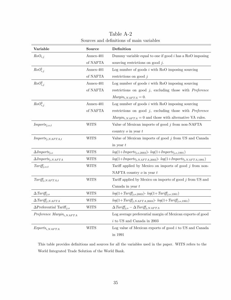
specified. The definition of the variables used in our empirical analysis and the sources

30We first average the preference margin across destination countries (Canada and the United States),for each final good i that imposes restriction on j. We then take the average across final goods. Giventhat the United States is by far the most important trading partner of Mexico, we have also tried touse a measure based on US tariffs only, obtaining similar results.

31Thus the effect of a RoO on final good i on imports of restricted input j does not depend on whetherCanada and the United States granted GSP preferences to Mexican producers of i before NAFTA.

32The ∆ variables thus represent percentage changes. Some variables y take values equal to zero. Inthese cases, we compute changes in log (1+y).

17

used to construct them can be found in Table A-2 in the Appendix.

In our benchmark regressions, we estimate

∆Importsj,o = α + β1 RoOxi,j + β2 ∆Preferential Tariffj,o + δj + δo + εj,o. (1)

This difference-in-differences approach allows us to remove any potential bias that could

be the result of time-invariant unobservable differences across goods. The dependent

variable, ∆Importsj,o, is the log change in Mexican imports of HS6-digit good j from non-

NAFTA country o between 1991 and 2003. The key regressor of interest is RoOxi,j, which

captures the effect of the introduction of NAFTA RoO on final goods i imposing sourcing

restrictions on intermediate j. As discussed in Section 4, we consider three versions of

the treatment variable RoOxi,j. In the first treatment (x = 1), we include all RoO on

final goods i imposing sourcing restrictions on good j. The second treatment (x = 2)

distinguishes the rules depending on the preference margin on the final good. This

measure excludes rules on final goods i for which the variable Preference Margini,NAFTA,

which producers have no incentives to comply with. The last treatment (x = 3) also

takes into account value added rules. This measure includes only rules for which the

preference margin on the final good is positive and for which there are no alternative

value added rules. We expect the estimated β1 coefficient to be negative and significant,

at least when using the more stringent treatment variables RoO2i,j and RoO3

i,j.

In all specifications, we include industry fixed effects δj (at HS3-digit level), which

allows us to control for sector-specific trends,33 as well as country-of-origin fixed effects,

which account for any country-specific determinants of Mexican imports (e.g. distance,

common language). In some specifications, we also include the variables ∆Preferential

Tariffj,o, the difference between the log change in the tariff applied by Mexico to imports

of good j from non-NAFTA country o and from NAFTA partners between 1991 and

2003. We expect the coefficient β2 to be negative, reflecting the trade diversion effect of

preferential tariff liberalization among NAFTA partners.

5.2 Baseline results (rules defined at 6 digits)

As mentioned in Section 4, some NAFTA RoO are defined at the chapter level (HS2),

others at the heading level (HS4) or sub-heading (HS6) level. In this section, we focus on

the impact of rules written at the HS6 level, which are more likely to identify vertically-

related goods (they apply to vertically-related goods in 96% of the cases). This allows

33For example, the inclusion of industry dummies accounts for sectoral changes in employment orproductivity, which may have affected Mexican imports from non-NAFTA countries.

18

us to have a more accurate measure of the treatment. In the next section, we show that

our results are robust to including rules defined at a more aggregate level.

Table 3 shows the results of estimating equation (1). In columns 1, 3 and 5, we report

the results of parsimonious specifications, in which we include only the RoO variables,

industry and country-of-origin fixed effects. In columns 2, 4 and 6, we also control for the

difference in the tariffs applied by Mexico to imports from third countries and NAFTA

partners.

Table 3NAFTA RoO and change in Mexican imports from non-NAFTA countries

(1) (2) (3) (4) (5) (6)

RoO1i,j 0.001 0.007

(0.086) (0.085)

RoO2i,j -0.267∗∗∗ -0.171∗∗

(0.083) (0.084)

RoO3i,j -0.306∗∗∗ -0.207∗∗

(0.084) (0.085)

∆Preferential Tariffj,o -0.574∗∗∗ -0.559∗∗ -0.555∗∗∗

(0.074) (0.084) (0.075)

Industry FE (HS3) yes yes yes yes yes yes

Country of origin FE yes yes yes yes yes yes

Observations 7,015 7,003 7,015 7,003 7,015 7,003

R-squared 0.244 0.252 0.245 0.252 0.245 0.252

This table shows the results of the estimation of equation (1). The dependent variable is

∆Importsj,o, the log change in Mexican imports of good j (defined at the HS 6-digit level) from

non-NAFTA country o between 1991 and 2003. The dependent variable includes goods for which

Mexican imports were positive in 1991 and 2003. RoOxi,j is the number (in logs) of final goods i

for which there is a NAFTA RoO restricting the sourcing of good j. When x = 1, the treatment

includes all final goods i. When x = 2, the treatment excludes rules associated to final goods i

for which Preference Margini,NAFTA = 0. When x = 3, the treatment further excludes change

of tariff classification rules that are combined with alternative value added rules. ∆Preferential

Tariffj,o is difference between the log change in the tariff applied by Mexico to imports of good j

from non-NAFTA country o and the log change in the tariff applied by Mexico to imports of good

j from NAFTA countries. Robust standard errors in parenthesis. Significance levels: ∗; 10%; ∗∗:

5%; ∗∗∗: 1%.

The key results of our analysis concern the coefficients of the RoO variables, which

capture the impact of NAFTA sourcing restrictions on Mexican imports of intermedi-

aries. Looking first at column 1 and 2, we find that the coefficient associated to RoO1i,j is

not insignificant. As discussed above, RoO on final goods should lead to trade diversion

in intermediaries only if the preference margin is positive. The fact that the coefficient

19

is insignificant in column (1) suggests that, by including in RoO1i,j final goods with zero

preference margin, we might be mis-measuring the treatment. Columns 3 and 4 show

that, when we use RoO2i,j as a treatment, our coefficient of interest becomes significant

at 1%. This finding confirms our prior: by including only final goods i for which the

variable Preference Margini,NAFTA is positive, we can isolate those RoO that constraint

producers’ sourcing decisions and better measure their effect on imports of intermediate

goods. In column 5 and 6, we use RoO3i,j to capture the impact of NAFTA sourcing

restrictions. This is our preferred treatment variable, because it only includes rules that

are relevant (final good producers have something to gain by complying to them) and

strict (origin can only be obtained if the restricted inputs are sourced within NAFTA).

Not surprisingly, the estimated coefficients for RoO3i,j are significant at 1% and larger

than for the weaker treatment variables.

How large was the trade diversion in intermediaries due to the introduction of

NAFTA sourcing restrictions? The estimate of column 6 in Table 3 indicates that

RoO of final goods decreased imports of affected intermediate goods from non-NAFTA

countries by around 26 percentage points.34 The effect was much larger for intermediate

goods that were subject to more sourcing restrictions. Consider for example the case of

“Other Positive Rotary Displacement Pumps” (HS6 841360). For this good, the variable

RoO3i,j was equal to 14, the 90th percentile in the distribution of treated goods. The

coefficient estimated in column 6 of Table 3 implies that NAFTA RoO reduced Mexican

imports from non-NAFTA by around 56 percentage points.

The results of Table 3 also confirm that NAFTA decreased imports from non-member

countries through a second more transparent channel, i.e. preferential tariff reduc-

tions vis-a-vis NAFTA partners. In columns 2, 4 and 6, the coefficient of the variable

∆Preferential Tariffj,o is negative and significant at 1%, indicating that the trade diver-

sion effect was larger in sectors characterized by larger reductions in Mexican tariffs on

imports from Canada and the United States relative to imports from third countries.35

In terms of magnitude, the estimated coefficient in column 6 indicates that preferential

tariff cuts vis-a-vis NAFTA partners decreased imports of intermediate goods from third

countries by around 155 percentage points.36

34The magnitude of the effect is obtained by multiplying the estimated coefficient of column 6 inTable 3 by the average of log RoO3

i,j (-0.207× 1.27 = −0.26). This reduction represents around 17% ofthe average actual change in imports of treated goods (0.26/1.53 = 0.17).

35Instead of ∆Preferential Tariffj,o ≡ ∆Tariffj,o −∆Tariffj,NAFTA, we can separately include in ourregressions the variables ∆Tariffj,o and ∆Tariffj,NAFTA. As expected, the estimated coefficients areboth negative and significant at 1%.

36The estimated coefficient of ∆Tariffj,o in column 6 of Table 3 is −0.55. The effect of input tariffs canbe computed multiplying this coefficient by the average of ∆Tariffj,o (−0.55∗2.8 = 1.55). The absolute

20

The results of Tables 3 should be considered as an underestimate of the effects of

RoO. There are two main reasons for this. First, in 2003 some Mexican producers

had still to fully understand and adjust to NAFTA sourcing restrictions.37 Second, in

our analysis so far, we have only looked at the impact of RoO that were written at

the sub-heading (HS6) level. As discussed in Section 4, these rules are more likely to

affect sourcing decisions, given that they apply to vertically-related goods in 96% of

the cases. By contrast, RoO defined at the chapter (HS2) and heading level (HS4)

apply to vertically-related goods in only 50% and 68% of the cases, respectively. By

excluding these rules, we have classified as “non treated” some intermediate goods that

were actually subject to sourcing restrictions. In the next section, we will extend the

analysis to NAFTA RoO defined at the chapter and heading level, exploiting information

from input-output tables to identify the rules that apply to vertically-related goods.

We next focus on intermediate goods that were subject to sourcing restrictions (i.e.

j goods for which the variable RoO3ij > 0) and exploit variation in the intensity of the

treatment. The negative impact of NAFTA RoO should be larger when Mexican final

good producers had stronger incentives to comply with them. The larger the difference

between the MFN and preferential tariffs applied by Canada and the United States

on their final goods, the stronger the incentives to source the restricted inputs within

NAFTA. The effect of RoO on Mexican imports of intermediaries from non-member

countries should thus be increasing in the variable Preference Margini,NAFTA.

The effect of NAFTA RoO should also have been more detrimental when the sourcing

restrictions apply to final goods for which Canada and the United States represent more

important export markets. To see this, consider the example of two Mexican producers,

selling different final goods. Before NAFTA, both producers some inputs from third

countries (e.g. Germany or Japan). Exports of the first producer were mostly destined

for the North American market, while the second producer exported more to the rest of

the world. Following the entry into force of the NAFTA agreement, the two producers

can export their goods to Canada and the United States at preferential rates, but only

if they stop importing certain inputs from third countries. NAFTA RoO should have a

stronger impact on the sourcing decisions of the first producer, who stands to gain more

from complying with them. The impact of RoO on Mexican imports of intermediate

goods j should thus depend on the importance of NAFTA export markets for Mexican

producers of final goods i. This is proxied by the variable Exportsi,NAFTA, the volume

value of this effect as a percentage of the change in imports of goods with RoO this is 1.55/1.53 = 1.01.37As mentioned before, many firms payed administrative and legal costs to comply with RoO, but

failed to obtain origin status (see footnote 17).

21

of pre-NAFTA (1991) Mexican exports of good i to Canada and the United States.

To verify these predictions, we run the following regression:

∆Importsj,o = α + β1 RoO3i,j × Preference Margini,NAFTA + β2 RoO3

i,j × Exportsi,NAFTA

+β3 RoO3i,j + β4 Preference Margini,NAFTA + β5 Exportsi,NAFTA

+β6 ∆Preferential Tariffj,o + δj + δo + εj,o. (2)

We expect trade diversion in intermediaries to be larger when final good producers have

stronger incentives to comply with NAFTA RoO. The estimated coefficients for β1 and

β2 should thus be negative and significant.

Table 4NAFTA RoO and change in Mexican imports from non-NAFTA countries

(1) (2) (3) (4) (5) (6)

RoO3i,j × Preference Margini,NAFTA -3.105 -3.780∗ -4.500∗∗ -5.615∗∗∗

(1.978) (2.017) 2.094 (2.167)

RoO3i,j × Exportsi,NAFTA -0.010∗ -0.021∗∗∗ -0.021∗∗ -0.023∗∗

(0.006) (0.007) (0.010) (0.010)

RoO3i,j 3.672 4.301∗ -1.334∗∗∗ -0.839∗∗ 5.548∗∗ 6.192∗∗

(2.364) (2.391) (0.365) (0.386) (2.592) (2.607)

Preference Margini,NAFTA 0.543 1.327 1.711 2.925∗

(1.522) (1.581) (1.648) (1.738)

Exportsi,NAFTA 0.056∗∗∗ 0.085∗∗∗ 0.062 0.079∗

(0.021) (0.024) (0.043) (.045)

∆Preferential tariffj,o -0.807∗∗ -0.700∗∗ -0.898∗∗

(0.383) (0.206) (0.397)

Industry FE (HS3) yes yes yes yes yes yes

Country of origin FE yes yes yes yes yes yes

Observations 348 346 600 598 348 346

R-squared 0.416 0.435 0.452 0.464 0.427 0.436

This table shows the results of the estimation of equation (2). The dependent variable is ∆Importsj,o, the

log change in Mexican imports of good j (defined at the HS 6-digit level) from non-NAFTA country o be-

tween 1991 and 2003. RoO3i,j is the number of final goods i that have a RoO restricting the sourcing of

good j, excluding those with Preference Margini,NAFTA = 0 and with alternative VA rules. The variable

Preference Margini,NAFTA is constructed based on the MFN and preferential tariffs applied by the US and

Canada in 2003. The variable Exportsi,NAFTA measures Mexican exports of final goods i to the US and

Canada in 1991. ∆Preferential Tariffj,o is difference between the log change in the tariff applied by Mexico to

imports of good j from non-NAFTA country o and the log change in the tariff applied by Mexico to imports

of good j from NAFTA countries. Significance levels: ∗; 10%; ∗∗: 5%; ∗∗∗: 1%.

The results are reported in Table 4. In all specifications, the interactions terms be-

tween the RoO variable and Preference Margini,NAFTA and Exportsi,NAFTA are negative

22

and significant. This confirms that the negative impact of NAFTA RoO on Mexican

imports of intermediate good j is larger when Mexican final good producers have more

to gain from obtaining origin status, i.e. when the preference margin is larger and

when NAFTA partners represent more important export markets. Based on the esti-

mates of Table 4, we can compute the effect of RoO for different levels of Preference

Margini,NAFTA and Exportsi,NAFTA. For example, the estimates in column (6) imply a

RoO coefficient of -3.01 for goods falling in the 90th percentile of the distribution of the

Preference Margini,NAFTA and a coefficient of -1.56 for goods in the 90th percentile of

the distribution of Exportsi,NAFTA.

In the Appendix, we report the results of additional estimations to verify the ro-

bustness of our main results. In our benchmark regressions, we include only goods that

Mexico imported from third countries in both 1991 and 2003. However, NAFTA sourcing

restrictions may have also affected whether or not Mexico imported at all a given inter-

mediate from non-member countries. To account for the effect of RoO on the extensive

margin, we reproduce all the specifications of Table 3, including in our analysis goods

that Mexico imported only in 1991 or 2003 (see Table A-3). The results confirm that

NAFTA RoO led to a reduction in Mexican imports of intermediaries from non-member

countries. As expected, the effect is stronger in columns 5 and 6, in which we consider

only change of classification rules that apply to final goods with a positive preference

margin and are not relaxed by alternative value added rules. We have also tried includ-

ing in our sample non-NAFTA countries that negotiated an FTA with Mexico during

our sample period (see Table A-4). The results continue to hold: NAFTA RoO had a

detrimental effect on Mexican imports of restricted inputs from third countries.38

5.3 Additional results (including rules defined at 2 and 4 digits)

RoO should only affect sourcing decisions if they apply to vertically-related goods, i.e.

if the restricted good j is actually used as an input in the production of final good i.

For this reason, in our analysis so far we have focused on RoO defined at the HS6 level,

which apply to vertically-related goods in almost 100% of the cases.39

38The sample used in these regressions includes EU members, Chile and Israel. As discussed inSection 4.2, for these countries, WITS provides data on the preferential tariffs applied by Mexico toimports from the FTA partners, which we can use to compute the variable ∆Preferential Tariffjo (seefootnote 28). Our analysis suggests that, to better explain changes in Mexican imports from these FTApartners, we would need to take into account the RoO contained in these trade agreements.

39Recall that, using information from input-output tables, we have computed the percentage ofNAFTA RoO defined at 2-, 4- and 6-digits of the HS classification restricting the sourcing of vertically-related goods (see Section 4.1). Rules defined at 6 digits apply to vertically-related goods in 96% of thecases. The number is much lower for rules defined at 2 and 4 digits (50% and 68%, respectively).

23

In this section, we show that the results continue to hold when we include RoO

defined at 2 and 4 digits. We follow three alternative approaches. First, we include all

rules, independently of vertical linkages. Second, we use information from input-output

tables to include only rules that apply to vertically-related goods. Finally, we allow the

impact of the rules to depend on the importance of the vertical linkages.

Table 5NAFTA RoO and change in Mexican imports from non-NAFTA countries

(including all rules)

(1) (2) (3) (4) (5) (6)

RoO1i,j -0.148∗ -0.080

(0.089) (0.088)

RoO2i,j -0.159∗∗ -0.096

(0.069) (0.069)

RoO3i,j -0.169∗∗∗ -0.112∗

(0.063) (0.063)

∆Preferential tariffj,o -0.567∗∗∗ -0.561∗∗∗ -0.554∗∗∗

(0.075) (0.075) (0.075)

Industry FE (HS3) yes yes yes yes yes yes

Country of origin FE yes yes yes yes yes yes

Observations 7,015 7,003 7,015 7,003 7,015 7,003

R-squared 0.244 0.252 0.244 0.252 0.245 0.252

This table shows the results of the estimation of equation (1). The dependent variable is

∆Importsj,o, the log change in Mexican imports of good j (defined at the HS 6-digit level) from

non-NAFTA country o between 1991 and 2003. The dependent variable includes goods for which

Mexican imports were positive in 1991 and 2003. RoOxi,j is the number (in logs) of final goods i

for which there is a NAFTA RoO restricting the sourcing of good j. When x = 1, the treatment

includes all final goods i. When x = 2, the treatment excludes rules associated to final goods i

for which Preference Margini,NAFTA = 0. When x = 3, the treatment further excludes change

of tariff classification rules that are combined with alternative value added rules. ∆Preferential

Tariffj,o is difference between the log change in the tariff applied by Mexico to imports of good j

from non-NAFTA country o and the log change in the tariff applied by Mexico to imports of good

j from NAFTA countries. Robust standard errors in parenthesis. Significance levels: ∗; 10%; ∗∗:

5%; ∗∗∗: 1%.

Table 5 reproduces the difference-in-differences specifications of Table 3, including

all rules contained in Annex 401 of the NAFTA agreement, independently of whether

or not they apply to vertically-related goods. Compared to our benchmark regressions,

here we account for the potential impact of all NAFTA RoO on Mexican imports of

intermediate goods. However, the treatment variables are less precisely measured, given

that many of the rules defined at 2 and 4 digits do not apply to vertically-related goods.

24

The results continue to hold. We find that NAFTA RoO on final goods led to a

reduction in Mexican imports of intermediaries from non-NAFTA countries. The effect

is significant only for rules that are relevant — apply to final goods with a positive

preference margin—and strict strict — are not relaxed by alternative value added rules.

In terms of magnitude, the estimated coefficient of column 6 in Table 5 implies that

RoO of final goods decreased intermediate imports from third countries by 32 percentage

points on average.40

Our next step is to exclude RoO that do not apply to vertically-related goods. To

check whether a given rule RoOij imposes a sourcing restriction, we must verify whether

good j is an input in the production of final good i. To this end, we exploit the infor-

mation contained in the IO Direct Requirement table 1997 provided by the BEA and

include in our treatment variables all rules for which dri,j > 0. Compared to the strategy

used in Table 5, this methodology allows us to eliminate from our treatment variables

RoO that do not impose any sourcing restrictions. However, the fact that IO tables are

RoO are written using different classifications (NAICS and HS) introduces some noise

in the measurement of vertical linkages. As discussed in Section 4.1, in the concordance

table provided by the BEA, each NAICS 6-digit good corresponds to more than one

HS 6-digit good. Imagine that, according to the concordance table, NAICS-6 good “a”

corresponds to HS6 goods “1” and “2”, and that NAICS-6 good “b” corresponds to HS6

goods “3” and “4”. To identify RoO that apply to vertically-related goods, we look

at the direct requirement coefficients of all matched NAICS-HS goods. If, for example,

NAICS 6-digit goods “a” and “b” are vertically related (i.e. dra,b > 0), we assume that

HS6 goods “1”, “2”, “3”, and “4” are all vertically related.

Using this methodology, in the regressions of Table 6 we exclude from our treatment

variables all rules that do not apply to vertically-related goods. Once again, we find a

negative relationship between the number of NAFTA sourcing restrictions applied to an

intermediate good and the change in Mexican imports of this good from non-member

countries. Once we control for the change in input tariffs, the effect is significant only

for rules with a positive preference margin and no alternative value added rules. The

effect is slightly smaller than in Table 5. The coefficient of RoO3 in column 6 implies

that NAFTA sourcing restrictions decreased Mexican imports of intermediaries by 18

percentage points.41

40This effect is computed by multiplying the estimated coefficient (−0.112) by the average of logRoO3

i,j for treated goods (2.839). This represents around 25% of the actual change in imports (computeddividing the 32 percentage points reduction by 1.246, the average log change in imports of treated goods.

41This reduction in imports is obtained by multiplying the estimated coefficient of column 6 in Table6 by the average of log RoO3

i,j (-0.069 × 2.65 = −0.18). This reduction represents around 15% of the

25

Table 6NAFTA RoO and change in Mexican imports from non-NAFTA countries

(including all rules for which dri,j > 0)

(1) (2) (3) (4) (5) (6)

RoO1i,j -0.058 -0.051

(0.041) (0.041)

RoO2i,j -0.026 -0.018

(0.038) (0.038)

RoO3i,j -0.082∗∗ -0.069∗

(0.041) (0.041)

∆Preferential tariffj,o -0.572∗∗∗ -0.573∗∗∗ -0.569∗∗∗

(0.074) (0.074) (0.074)

Industry FE (HS3) yes yes yes yes yes yes

Country of origin FE yes yes yes yes yes yes

Observations 7,015 7,003 7,015 7,003 7,015 7,003

R-squared 0.244 0.252 0.244 0.252 0.244 0.252

This table shows the results of the estimation of equation (1). The dependent variable is

∆Importsj,o, the log change in Mexican imports of good j (defined at the HS 6-digit level)

from non-NAFTA country o between 1991 and 2003. The dependent variable includes goods

for which Mexican imports were positive in 1991 and 2003. The variable RoOxi,j is the number

(in logs) of rules RoOi,j , weighted by the dri,j coefficients. When x = 1, the treatment includes

all final goods i. When x = 2, the treatment excludes rules associated to final goods i for which

Preference Margini,NAFTA = 0. When x = 3, the treatment further excludes change of tariff

classification rules that are combined with alternative value added rules. ∆Preferential Tariffj,o

is difference between the log change in the tariff applied by Mexico to imports of good j from

non-NAFTA country o and the log change in the tariff applied by Mexico to imports of good

j from NAFTA countries. Robust standard errors in parenthesis. Significance levels: ∗; 10%;∗∗: 5%; ∗∗∗: 1%.

The effect of RoO on imports of intermediaries may vary across final goods. Consider,

for example, two rules applying to final goods i and i′, both imposing sourcing restrictions

on intermediate good j. Suppose that j is a more important input in the production of

the first final good (i.e. dri,j > dri′,j). The effect of RoOi,j may be larger than the effect

of RoOi′,j, if the costs of switching to NAFTA suppliers is lower for i producers (which

could be the case if final good producers face fixed costs of searching for new suppliers).

The opposite may be true if the switching costs are higher for i producers (which could

be the case if higher dr coefficients proxy for higher quality inputs).42.

average change in imports of goods subject to sourcing restrictions (0.18/1.53 = 0.15).42The effect of RoO may also vary across different inputs. For example, RoO that apply to final

good i may restrict the sourcing of two different intermediate goods, j and j′. Suppose that j is a more

26

Table 7NAFTA RoO and change in Mexican imports from non-NAFTA countries

(weighting rules by dri,j)

(1) (2) (3) (4) (5) (6)

RoO1i,j -0.102 -0.116

(0.087) (0.088)

RoO2i,j -0.124 -0.130

(0.090) (0.091)

RoO3i,j -0.328∗∗∗ -0.317∗∗

(0.123) (0.124)

∆Preferential tariffj,o -0.576∗∗∗ -0.575∗∗∗ -0.571∗∗∗

(0.074) (0.074) (0.074)

Industry FE (HS3) yes yes yes yes yes yes

Country of origin FE yes yes yes yes yes yes

Observations 7,015 7,003 7,015 7,003 7,015 7,003

R-squared 0.244 0.252 0.244 0.252 0.245 0.253

This table shows the results of the estimation of equation (1). The dependent variable is

∆Importsj,o, the log change in Mexican imports of good j (defined at the HS 6-digit level)

from non-NAFTA country o between 1991 and 2003. The dependent variable includes goods

for which Mexican imports were positive in 1991 and 2003. The variable RoOxi,j is the number

(in logs) of rules RoOi,j , weighted by the dri,j coefficients. When x = 1, the treatment includes

all final goods i. When x = 2, the treatment excludes rules associated to final goods i for which

Preference Margini,NAFTA = 0. When x = 3, the treatment further excludes change of tariff

classification rules that are combined with alternative value added rules. ∆Preferential Tariffj,o

is difference between the log change in the tariff applied by Mexico to imports of good j from

non-NAFTA country o and the log change in the tariff applied by Mexico to imports of good j

from NAFTA countries. Robust standard errors in parenthesis. Significance levels: ∗; 10%; ∗∗:

5%; ∗∗∗: 1%.

To allow for these heterogeneous effects, we modify our treatment variables, weight-

ing each rule RoOij by the direct requirement coefficient drij. Table 7 reproduces our

difference-in-differences regressions when we use these alternative RoO regressors. Once

again, we find that NAFTA RoO reduced Mexican imports of intermediaries from non-

NAFTA countries. As in previous specifications, we also find that the effect is significant

only for RoO3. In terms of magnitude, the estimate in column 6 implies an average re-

duction in imports of affected intermediate goods of around 19 percentage points.43

important input in the production of i (i.e. dri,j > dri,j′). We would then expect Mexican imports of jto exceed imports of j′ both pre-and post-NAFTA. This type of heterogeneity is already accounted forin our empirical analysis: our dependent variable is expressed in percentage changes (log differences),so we already control for differences in the level of j and j′ imports.

43As before, this percentage points reduction in imports is obtained by multiplying the estimated

27

In this section we have shown that results on the effects of NAFTA RoO are ro-

bust to (i) including all rules, (ii) excluding rules that do not apply to vertically-related

goods, and (iii) taking into account the importance of the input-output linkages when

constructing our treatment variables. Our results show that preferential RoO on final

goods negatively affect imports of intermediaries from non-member countries. Not sur-

prisingly, the effect of RoO depends on whether final good producers have incentives to

comply with the sourcing restrictions and whether these are strict or flexible. In terms

of magnitude, the effect is quite stable across specifications. In the baseline regressions

in which we include all rules, imports of goods subject to sourcing restrictions fell by

more than 30 percentage points. In the other specifications, imports of restricted goods

feel by around 20 percentage points.

5.4 Instrumenting NAFTA rules with CUSFTA rules

As mentioned earlier, our focus on Mexico is due to the fact that NAFTA RoO were to

a large extent inherited from those contained in the Canada-United States Free Trade

Agreement (CUSFTA). The sourcing restrictions embedded in Annex 401 of the NAFTA

agreement can thus be considered as exogenous to Mexican final good producers.

To deal with any remaining endogeneity concerns, we next use the RoO contained in

the CUSFTA agreement to instrument for NAFTA RoO. We argue that CUSFTA RoO

satisfy the two requirements of an instrument. First, the extent to which the sourcing of

a given intermediate good was restricted by CUSFTA RoO is unlikely to be correlated

with any residual in equation (1). Second, the rules contained in the two agreements

are highly correlated, which makes the instrument very strong: the correlation between

the dummy variable RoOij in the two agreements is 0.91; the correlation between the

treatment variables is 0.97 for RoO1 and RoO2, and 0.98 for RoO3.44

Table 8 shows the results of estimating equation (1), when we instrument NAFTA

RoO with their CUSFTA counterparts.45 The first-stage coefficients associated to CUS-

FTA RoO1, RoO2 and RoO3 are 0.66, 0.79, and 0.85 respectively. The three of them

are statistically significant at 1%. As column (6) indicates, the effect of RoO on imports

of intermediate goods remains negative and significant. The coefficients are larger and

more precisely estimated than their OLS counterparts (see Table 5).coefficient of column 6 in Table 7 by the average of log RoO3

i,j (-0.317×0.63 = −0.20). The absolute valueof this effect as a percentage of the average change in imports of restricted goods is 0.20/1.23 = 0.16.

44We have performed the Hausman test by including as a regressor the residuals of the first stage inthe OLS regression. Endogeneity of the instrument is rejected at the 1% level in all cases.

45In this section, we report the IV results using all rules. The results continue to hold if we consideronly those rules defined at the HS-6 level in CUSFTA and NAFTA.

28

Table 8NAFTA RoO and change in Mexican imports from non-NAFTA countries

(Instrumenting NAFTA rules with CUSFTA rules)

(1) (2) (3) (4) (5) (6)

RoO1i,j -0.093 -0.098

(0.138) (0.135)

RoO2i,j -0.270∗∗∗ -0.167∗∗

(0.081) (0.081)

RoO3i,j -0.298∗∗∗ -0.199∗∗

(0.074) (0.074)

∆Preferential Tariffj,o -0.566∗∗∗ -0.552∗∗∗ -0.544∗∗∗

(0.075) (0.075) (0.074)

Industry FE (HS3) yes yes yes yes yes yes

Country of origin FE yes yes yes yes yes yes

Observations 7,015 7,003 7,015 7,003 7,015 7,003

R-squared 0.245 0.252 0.245 0.252 0.245 0.252

This table shows the results of the estimation of equation (1). The dependent variable is

∆Importsj,o, the log change in Mexican imports of good j (defined at the HS 6-digit level) from

non-NAFTA country o between 1991 and 2003. The dependent variable includes goods for which

Mexican imports were positive in 1991 and 2003. RoOxi,j is the number (in logs) of final goods i for

which there is a NAFTA RoO restricting the sourcing of good j, instrumented using CUSFTA RoO.

When x = 1, the treatment includes all final goods i. When x = 2, the treatment excludes rules

associated to final goods i for which Preference Margini,NAFTA = 0. When x = 3, the treatment

further excludes change of tariff classification rules that are combined with alternative value added

rules. ∆Preferential Tariffj,o is difference between the log change in the tariff applied by Mexico to

imports of good j from non-NAFTA country o and the log change in the tariff applied by Mexico

to imports of good j from NAFTA countries. Robust standard errors in parenthesis. Significance

levels: ∗; 10%; ∗∗: 5%; ∗∗∗: 1%.

6 Conclusions

Recent decades have witnessed a proliferation of free trade agreements. Preferential

rules of origin (RoO) are a key element in the functioning of these agreements: they

determine the conditions that a product must satisfy to be considered as originating

from the member countries and receive preferential tariff treatment.

Theoretical studies have long pointed out that RoO can give rise to trade diversion

in intermediaries (e.g. Grossman, 1981; Falvey and Reed, 1998). The distortive effect of

these sourcing restrictions is also emphasized in recent surveys. For example, in a study

by the International Trade Centre (2015) based on large-scale surveys of companies in

29

developing countries, RoO emerge as the most problematic non-tariff measure faced by

manufacturing firms.

However, systematic empirical evidence about the impact of RoO has been lacking,

due to their legal complexity, which makes measurement difficult. We have overcome

this difficulty by focusing on NAFTA, the world’s largest FTA. Thanks to the specific

legal features of Annex 401, we have been able to construct a unique dataset, which

allows to trace input-output linkages in NAFTA RoO: for each final good, we can trace

all the intermediate goods that are subject to sourcing restrictions; similarly, for every

intermediate good, we can trace all the final goods that impose RoO restrictions on its

sourcing.

NAFTA RoO were to a large extent inherited from those of its predecessor, the

Canada-United States Free Trade Agreement (the correlation between the rules con-

tained in the two agreements is 0.91). They can thus be considered as exogenous from

the point of view of Mexico, the country we focus our analysis on. Using a difference-

in-differences approach, we find that NAFTA RoO had a negative impact on Mexican

imports of intermediaries from third countries. The effect is sizable: in our preferred

specification based on rules defined at 6 digits, imports of restricted goods decreased by

26 percentage points on average; the corresponding effect is 32 percentage points when

we include all rules. The magnitude of the effect depends also on whether the rules are

strict or flexible, and on the incentives of final good producers to comply with them —

which, in turn, depend on the extent of the preference margin and the importance of

NAFTA export markets.

Our analysis has allowed us to identify the negative impact of the sourcing restrictions

embedded in free trade agreements (FTAs) on imports of intermediaries from non-FTA

members. An important avenue of future research is to quantify the impact of FTAs

on aggregate productivity and welfare, through their effect of firms’ sourcing decisions.

To this purpose, we could include preferential tariffs and RoO in a model of global

sourcing a la Antras et al. (2014) and combine our dataset on NAFTA RoO with

tariff data and Mexican firm-level trade data before and after NAFTA. Collecting firm-

level data would also allow us to study the trade creation effects of NAFTA RoO and

verify whether Mexican imports of intermediaries from third countries were displaced

by inputs produced domestically or imported from Canada and the United States.It

would also be interesting to study whether NAFTA sourcing restrictions led foreign

suppliers to relocated within the FTA. Identifying this “RoO-jumping” effect would

require disaggregated data on Mexican inward FDI.

It is well known that input tariffs are low compared to tariffs on final goods (e.g.

30

Miroudot et al., 2009). Our results show that, when accounting for the sourcing restric-

tions embedded in preferential trade agreements, the actual level of protection on these

goods is much higher. Our analysis also suggests that many FTAs, including NAFTA,

violate multilateral trade rules. Paragraph 5 (b) of Article XXIV of the GATT states

that “the duties and other regulations of commerce maintained in each of the constituent

territories and applicable at the formation of such free-trade area” (. . . ) “shall not be

higher or more restrictive than the corresponding duties and other regulations of com-

merce existing in the same constituent territories prior to the formation of the free trade

area”. Our findings show that, through their preferential RoO, FTAs can substantially

increase the level of protection faced by non-members.

References

Alfaro, L., P. Antras, D. Chor, and P. Conconi (2015). “Internalizing Global Value

Chains: A Firm-Level Analysis” , NBER Working Paper 21582.

Alfaro, L., P. Conconi, H. Fadinger, and A. Newman (2014). “Do Prices Determine

Vertical Integration?” , Review of Economic Studies, forthcoming.

Antras, P., and D. Chor (2013). “Organizing the Global Value Chain,” Econometrica

81, 2127-2204.

Antras, P., D. Chor, T. Fally, and R. Hillberry (2012). “Measuring the Upstreamness of

Production and Trade Flows,” American Economic Review Papers & Proceedings

102. 412-416.

Antras, P., T. Fort, and F. Tintelnot (2014). “The Margins of Global Sourcing: Theory

and Evidence from U.S.”, mimeo.

Blackhurst, R., A. Enders, and J. F. Francois (1996). “The Uruguay Round and Market

Access: Opportunities and Challenges for Developing Countries,” in W. Martin

and L. A. Winters (eds.), The Uruguay Round and the Developing Countries,

Cambridge University Press.

Bombarda, P., and E. Gamberoni (2013). “Firm Heterogeneity, Rules of Origin and

Rules of Cumulation,” International Economic Review 54, 307-328.

Bown, C. P., and M. A. Crowley (2006). “Policy Externalities: How US Antidumping

Affects Japanese Exports to the EU,” European Journal of Political Economy 22:

696-714.

Bown, C. P., and M. A. Crowley (2007). “Trade Deflection and Trade Depression,”

Journal of International Economics 72: 176-201.

31

Blaum, J., C. Lelarge, and M. Peters (2013). “Estimating the Productivity Gains from

Importing,” mimeo.

Caliendo, L., and F. Parro (2015). “Estimates of the Trade and Welfare Effects of

NAFTA,” Review of Economic Studies 82, 1-44.

Chang, W. and A. L. Winters (2002). “How Regional Blocs Affect Excluded Countries:

The Price Effects of MERCOSUR,” American Economic Review 92, 889-904.

Chase, Kerry A. (2008). “Protecting Free Trade: The Political Economy of Rules of

Origin,” International Organization 62, 507-530.

Carrere , C., and J. de Melo (2006). “Are different rules of origin equally costly?

estimates from NAFTA,” in O. Cadot, A. Estevadeordal, A. Suwa-Eisenmann

and T. Verdier (eds.) The origin of goods - Rules of Origin in Regional Trade

Agreements Oxford University Press, 191-212.

Dixit, A. K., and Grossman, G. M. (1982). “Trade and Protection with Multistage

Production,” Review of Economic Studies 49, 583-594.

Duttagupta, R., and A. Panagariya (2007). “Free Trade Areas and Rules of Origin:

Economics and Politics,” Economics and Politics 19, 169-190.

Eaton, J., and S. S. Kortum (2002). “Technology, Geography, and Trade,?” Economet-

rica 70, 1741-1779.

Estevadeordal, A. (2000). “Negotiating Preferential Market Access: The Case of the

North American Free Trade Agreement,” Journal of World Trade 34, 141-166.

Estevadeordal, A., and K. Suominem (2006). “Mapping and measuring rules of origin

around the world,” in O. Cadot, A. Estevadeordal, A. Suwa-Eisenmann and T.

Verdier (eds.) The origin of goods - Rules of Origin in Regional Trade Agreements

Oxford University Press, 69-113.

Falvey, R., and G. Reed (1998). “Economic Effects of Rules of Origin,” Review of World

Economics, 134, 209-229.

Grossman, G. M. (1981). “The Theory of Domestic Content Protection and Content

Preference, Quarterly Journal of Economics 96, 583-603.

Grossman, G., and E. Helpman (1995). “The Politics of Free Trade Agreements,”

American Economic Review 85, 667-690.

International Trade Centre (2015). “The Invisible Barriers to Trade: How Businesses

Experience Non-Tariff Measures.”

Johnson, R. C. and G. Noguera (2012). “Accounting for Intermediates: Production

Sharing and Trade in Value Added,” Journal of International Economics 86, 224-

236.

32

Ju, J., and K. Krishna (2005). “Firm behavior and Market Access in a Free Trade

Area,” Canadian Journal of Economics 38, 290-308.

Kee, H. L., and H. Tangi (2013). ¿‘Domestic Value Added in Exports: Theory and Firm

Evidence from China,” ?American Economic Review, forthcoming.

Koopman, R., Z. Wang, and S-J Wei (2013). ¿‘Tracing Value-Added and Double Count-

ing in Gross Exports,” ?American Economic Review, forthcoming.

Kehoe, T., and K. Ruhl (2013). “How Important is the New Goods Margin in Interna-

tional Trade?,” Journal of Political Economy 121(2), 358-392.

Koopman, R., Z. Wang, and S-J Wei (2013). ¿‘Tracing Value-Added and Double Count-

ing in Gross Exports,” ?American Economic Review, forthcoming.

Krishna, K., and A. O. Krueger (1995). “Implementing Free Trade Areas: Rules of

Origin and Hidden Protection,” in A. Deardorff, J. Levinsohn and R. Stern (eds.),

New Directions in Trade Theory, University of Michigan Press.

Miroudot, S. , Lanz, R. and A. Ragoussis (2009). “Trade in Intermediate Goods and

Services,” OECD Trade Policy Working Paper 93.

Puccio, L. (2013). Building Bridges between Regionalism and Multilateralism: Enquiries

on the Ways and Means to Internationally Regulate Rules of Origin and their

Impact on Systemic Problems of FTA. EUI Thesis - Cadmus Repository, 355.

Ramanarayanan, A. (2014). “Imported Inputs and the Gains from Trade,” mimeo.

Vermulst, E. A. (1992). “Rules of Origin as Commercial Policy Instruments - Revisited,”

Journal of World Trade 26, 61-102.

Vousden, N. (1987). “Content Protection and Tariffs under Monopoly and Competi-

tion,” Journal of International Economics 23, 263-282.

Winters, A. L., and W. Chang (2000). “Regional Integration and Import Prices: an

Empirical Investigation,” Journal of International Economics 51, 363-377.

Villarreal, M. A. (2010). “NAFTA and the Mexican Economy,” CRS Report for

Congress R40784.

33

Appendix

Table A-1Countries included in our empirical analysis

Africa Europe Asia America Oceania

Angola Albania Bahrain Antigua and Barbuda AustraliaBenin Armenia Bangladesh Barbados BruneiBotswana Bulgaria Cambodia Belize FijiBrunei Croatia China Canada New ZealandBurkina Faso Cyprus Egypt, Arab Rep. Chile Papua New GuineaBurundi Estonia Hong Kong, China Dominica Solomon IslandsCameroon EU (2003) countries India Dominican Republic TongaCape Verde Georgia Indonesia El SalvadorCentral African Republic Hungary Israel GrenadaChad Latvia Japan GuyanaCongo, Dem. Rep Lithuania Jordan HaitiCongo, Rep. Macedonia, FYR Korea, Rep. HondurasCote d’Ivoire Malta Kuwait JamaicaDjibouti Moldova Kyrgyz Republic Netherlands AntillesGabon Poland Malaysia SurinameGambia, The Slovak Republic Maldives Trinidad and TobagoGhana Slovenia Mongolia United StatesGuinea Turkey MyanmarGuinea-Bissau Tunisia NepalKenya Ukraine OmanLesotho PakistanMacao PhilippinesMadagascar QatarMalawi Saudi ArabiaMali SingaporeNiger Sri LankaNigeria Taiwan, ChinaSenegal ThailandSierra Leone United Arab EmiratesSouth Africa VietnamSwazilandTanzaniaTogoUgandaZambiaZimbabweNamibiaMozambiqueMoroccoMozambiqueMoroccoMauritus

This table lists all countries for which Mexico reported positive imports in 1991 and/or 2003, excluding

countries which during our sample period had i) free trade agreements with Mexico, for which data on

preferential tariffs are not available or ii) partial scope trade agreements with Mexico.

34

Table A-2Sources and definitions of main variables

Variable Source Definition

RoOi,j Annex-401 Dummy variable equal to one if good i has a RoO imposing

of NAFTA sourcing restrictions on good j.

RoO1i,j Annex-401 Log number of goods i with RoO imposing sourcing

of NAFTA restrictions on good j

RoO2i,j Annex-401 Log number of goods i with RoO imposing sourcing

of NAFTA restrictions on good j, excluding those with Preference

Margini,NAFTA = 0.

RoO3i,j Annex-401 Log number of goods i with RoO imposing sourcing

of NAFTA restrictions on good j, excluding those with Preference

Margini,NAFTA = 0 and those with alternative VA rules.

Importsj,o,t WITS Value of Mexican imports of good j from non-NAFTA

country o in year t

Importsj,NAFTA,t WITS Value of Mexican imports of good j from US and Canada

in year t

∆Importsj,o WITS log(1+Importsj,o,2003)- log(1+Importsj,o,1991)

∆Importsj,NAFTA WITS log(1+Importsj,NAFTA,2003)- log(1+Importsj,NAFTA,1991)

Tariffj,o,t WITS Tariff applied by Mexico on imports of good j from non-

NAFTA country o in year t

Tariffj,NAFTA,t WITS Tariff applied by Mexico on imports of good j from US and

Canada in year t

∆Tariffj,o WITS log(1+Tariffj,o,2003)- log(1+Tariffj,o,1991)

∆Tariffj,NAFTA WITS log(1+Tariffj,NAFTA,2003)- log(1+Tariffj,o,1991)

∆Preferential Tariffj,o WITS ∆Tariffj,o −∆Tariffj,NAFTA

Preference Margini,NAFTA Log average preferential margin of Mexican exports of good

i to US and Canada in 2003

Exportsi,NAFTA WITS Log value of Mexican exports of good i to US and Canada

in 1991

This table provides definitions and sources for all the variables used in the paper. WITS refers to the

World Integrated Trade Solution of the World Bank.

35

Table A-3NAFTA RoO and change in Mexican imports from non-NAFTA countries

(including zero imports)

(1) (2) (3) (4) (5) (6)

RoO1i,j 0.003 0.005

(0.044) (0.044)

RoO2i,j -0.141∗∗∗ -0.085∗∗

(0.044) (0.044)

RoO3i,j -0.156∗∗∗ -0.096∗∗

(0.045) (0.046)

∆Preferential tariffj,o -0.328∗∗∗ -0.319∗∗∗ -0.318∗∗∗

(0.040) (0.040) (0.040)

Industry FE (HS3) yes yes yes yes yes yes

Country of origin FE yes yes yes yes yes yes

Observations 29,057 28,067 29,057 28,067 29,057 28,067

R-squared 0.208 0.217 0.208 0.217 0.208 0.217

This table shows the results of the estimation of equation (1). The dependent variable is

∆Importsj,o, the log change in Mexican imports of good j (defined at the HS 6-digit level) from

non-NAFTA country o between 1991 and 2003. The dependent variable includes goods for which

Mexican imports were positive in 1991 and/or 2003. RoOxi,j is the number (in logs) of final goods

i for which there is a NAFTA RoO restricting the sourcing of good j. When x = 1, the treatment

includes all final goods i. When x = 2, the treatment excludes rules associated to final goods i

for which Preference Margini,NAFTA = 0. When x = 3, the treatment further excludes change

of tariff classification rules that are combined with alternative value added rules. ∆Preferential

Tariffj,o is difference between the log change in the tariff applied by Mexico to imports of good j

from non-NAFTA country o and the log change in the tariff applied by Mexico to imports of good

j from NAFTA countries. Robust standard errors in parenthesis. Significance levels: ∗; 10%; ∗∗:

5%; ∗∗∗: 1%.

36

Table A-4NAFTA RoO and change in Mexican imports from non-NAFTA countries

(including Mexico’s FTA partners)

(1) (2) (3) (4) (5) (6)

RoO1i,j -0.011 -0.011

(0.045) (0.045)

RoO2i,j -0.106∗∗ -0.086∗

(0.044) (0.044)

RoO3i,j -0.119∗∗∗ -0.098∗∗

(0.046) (0.046)

∆Preferential tariffj,o -0.155∗∗∗ -0.149∗∗∗ -0.148∗∗∗

(0.042) (0.042) (0.042)

Industry FE (HS3) yes yes yes yes yes yes

Country of origin FE yes yes yes yes yes yes

Observations 17,547 17,531 17,547 17,531 17,547 17,535

R-squared 0.139 0.140 0.139 0.140 0.139 0.146

This table shows the results of the estimation of equation (1). The dependent variable is

∆Importsj,o, the log change in Mexican imports of good j (defined at the HS 6-digit level) from

non-NAFTA country o between 1991 and 2003. The dependent variable includes goods for which

Mexican imports were positive in 1991 and 2003. RoOxi,j is the number (in logs) of final goods i

for which there is a NAFTA RoO restricting the sourcing of good j. When x = 1, the treatment

includes all final goods i. When x = 2, the treatment excludes rules associated to final goods i

for which Preference Margini,NAFTA = 0. When x = 3, the treatment further excludes change

of tariff classification rules that are combined with alternative value added rules. ∆Preferential

Tariffj,o is difference between the log change in the tariff applied by Mexico to imports of good j

from non-NAFTA country o and the log change in the tariff applied by Mexico to imports of good

j from NAFTA countries. Robust standard errors in parenthesis. Significance levels: ∗; 10%; ∗∗:

5%; ∗∗∗: 1%.

37

Figure A-1NAFTA RoO