From Numerical Analysis to Computational Science Bj¨ orn Engquist · Gene Golub 1. Introduction The modern development of numerical computing is driven by the rapid in- crease in computer performance. The present exponential growth approximately follows Moore’s law, doubling in capacity every eighteen months. Numerical computing has, of course, been part of mathematics for a very long time. Al- gorithms by the names of Euclid, Newton and Gauss, originally designed for computation “by hand”, are still used today in computer simulations. The electronic computer originated from the intense research and devel- opment done during the second world war. In the early applications of these computers the computational techniques that were designed for calculation by pencil and paper or tables and mechanical machines were directly implemented on the new devices. Together with a deeper understanding of the computational processes new algorithms soon emerged. The foundation of modern numerical analysis was built in the period from the late forties to the late fifties. It be- came justifiable to view numerical analysis as an emerging separate discipline of mathematics. Even the name, numerical analysis, originated during this pe- riod and was coined by the National Bureau of Standards in the name of its laboratory at UCLA, the Institute for Numerical Analysis. Basic concepts in numerical analysis became well defined and started to be understood during this time: • numerical algorithm • iteration and recursion • stability • local polynomial approximation • convergence • computational complexity The emerging capability of iteratively repeating a set of computational op- erations thousands or millions of times required carefully chosen algorithms. A theory of stability became necessary. All of the basic concepts were important but the development of the new mathematical theory of stability had the most immediate impact. The pioneers in the development of stability theory for finite difference approximations of partial differential equations were von Neumann, Lax and Kreiss, see e.g. the text by Richtmyer and Morton [16]. In numerical linear algebra the early analysis by Wilkinson was fundamental, [19] and the paper Page: 433 Engquist/Schmid (eds.) Mathematics Unlimited – 2001 and Beyond author: Engquis2 date/time: 29-Oct-2000 / 19:48
Transcript
From Numerical Analysisto Computational ScienceBjorn Engquist · Gene Golub
1. Introduction
The modern development of numerical computing is driven by the rapid in-crease in computer performance. The present exponential growth approximatelyfollows Moore’s law, doubling in capacity every eighteen months. Numericalcomputing has, of course, been part of mathematics for a very long time. Al-gorithms by the names of Euclid, Newton and Gauss, originally designed forcomputation “by hand”, are still used today in computer simulations.
The electronic computer originated from the intense research and devel-opment done during the second world war. In the early applications of thesecomputers the computational techniques that were designed for calculation bypencil and paper or tables and mechanical machines were directly implementedon the new devices. Together with a deeper understanding of the computationalprocesses new algorithms soon emerged. The foundation of modern numericalanalysis was built in the period from the late forties to the late fifties. It be-came justifiable to view numerical analysis as an emerging separate disciplineof mathematics. Even the name, numerical analysis, originated during this pe-riod and was coined by the National Bureau of Standards in the name of itslaboratory at UCLA, the Institute for Numerical Analysis. Basic concepts innumerical analysis became well defined and started to be understood duringthis time:
• numerical algorithm• iteration and recursion• stability• local polynomial approximation• convergence• computational complexity
The emerging capability of iteratively repeating a set of computational op-erations thousands or millions of times required carefully chosen algorithms. Atheory of stability became necessary. All of the basic concepts were importantbut the development of the new mathematical theory of stability had the mostimmediate impact.
The pioneers in the development of stability theory for finite differenceapproximations of partial differential equations were von Neumann, Lax andKreiss, see e.g. the text by Richtmyer and Morton [16]. In numerical linearalgebra the early analysis by Wilkinson was fundamental, [19] and the paper
[7] by Dahlquist gave the foundation for stability and convergence theory ofnumerical methods for ordinary differential equations.
The development of numerical computing has been gradual and based on theimprovements of both algorithms and computers. Therefore, labeling differentperiods becomes somewhat artificial. However, it is still useful to talk about anew area, often called scientific computing, which developed a couple of decadesafter the foundation of numerical analysis. The SIAM Journal of Scientific andStatistical Computing was started in 1980.
Numerical analysis has always been strongly linked to mathematics, appli-cations and the computer. It is a part of applied mathematics and its languageis mathematics. Its purpose is to solve real world problems from basic physicsto practical engineering. The tool used to obtain the solution is the computer.Thus its development is often driven by technology, both in terms of computercapacity and architecture and also by the many technological applications. Withthe term scientific computing we indicate a further strengthening of these links.It, therefore, became less viable to think of numerical computing as an isolatedtopic.
As the mathematical models to be numerically approximated became morecomplex, more advanced mathematical analysis was necessary. The emphasisshifted from linear to nonlinear problems, and it became possible to handlemore realistic applications. Yet, in order to construct efficient algorithms forthese applications, a more detailed knowledge of their properties was needed.The computer architecture changed. Vector and parallel architectures requireda rethinking of the basic algorithms. The powerful new computers also pro-duced enormous amounts of data and consequently visualization became moreimportant in order to understand the results of the calculations.
We use the label computational science for the latest shift in paradigms, thatis now occuring at the turn of the century. The links to the rest of mathematics, toapplication and the rest of the computer science are even further strengthened.However, the most significant change is that new fields of applications are beingconsidered.
We use the label computationalscience for the latest shift inparadigms, that is now occuringat the turn of the century.
Many important parts of numerical computing were established with littleinput from mathematicians specializing in numerical analysis or scientific com-puting. This includes simulations in large parts of physics, chemistry, biologyand material science. The scientists in these fields often developed their ownalgorithms. It is clear that it is of mutual benefit for both the scientists and theexperts in numerical analysis to initiate closer collaboration. The applied math-ematicians can analyze and improve the numerical methods and also adapt themto new areas of applications. This has happened in many fields in the past. Math-ematical analysis has been the basis for the derivation of new algorithms, whichoften have contributed more to the overall computational capability than theincrease in computer power. Computational science has also been a stimulatingsource for new problems in mathematics.
2. Two Computational Subfields
We shall discuss the two important fields of numerical linear algebra and com-putational fluid dynamics. The computer can only do logical and basic arith-
From Numerical Analysis to Computational Science 435
metical operations. Therefore the core of all numerical computation will be tosolve problems from linear algebra. Numerical linear algebra reached a maturestate quite early in terms of theory and software. It is, however, still developingpartly because it is very sensitive to changes in computer architecture.
The field of computational fluid dynamics has been a significant engine forthe development of numerical computing throughout the century. The reasonhas been the importance of applications such as weather prediction and aerody-namical simulations, but also the relative complexity of nonlinear mathematicalmodels requiring careful analysis in the development of numerical algorithms.
2.1 Numerical Linear Algebra
From the earliest days of modern electronic computers, the solution of partialdifferential equations and matrix equations have been of great interest and im-portance. Solving systems of equations was often a central issue in solving asparse system associated with an approximation to a partial differential equa-tion. There was significant interest in the solution of linear equations for suchproblems which often arise in scientific and engineering applications, as wellas in statistical problems. There has been from the earliest days a considerableeffort in solving numerical problems arising in linear algebra, a pursuit whichhas involved such distinguished mathematicians as von Neumann and Turing.However, the number of people involved in this effort has always been relativelysmall, probably less than 150 people at any given time. This estimate is based onthe attendance at the Householder meetings which is held approximately everythree years and is devoted to numerical linear algebra.
There are three important components that play a role in solving any prob-lem involving linear algebra. They are: perturbation theory, development andanalysis of numerical algorithms and software. We shall briefly describe someof the developments in each of these areas which has taken place in the last fiftyyears.
Let us consider a system of equations
Ax = b + r
where A is an m × n matrix, and b is a given vector. We desire to determinex so that the norm ‖r‖ = min. There are several “parameters” associated withthe numerical solution of such a problem. We list some of these below.
a) The relationship between m and n is of importance in any numerical proce-dure. Whenm ≥ n, then the system is overdetermined, but in many instances,the solution will be unique.
b) The rank of the matrix A may or may not be known explicitly. The realdifficulty arises when a small perturbation in A will change the rank.
c) The numerical algorithms will be dependent on the norm chosen. For instancewhen the least squares solution is computed, it is only necessary to solve asystem of linear equations, though this can have disastrous effects!
d) The structure of the matrixA plays an important role in any solution method.If the matrix, for example, is sparse or symmetric, specialized methods maybe used.
e) Another important consideration is the origin of the problem. For instance,if one is solving the approximation of an elliptic equation, then often onecan make use of this knowledge in developing an algorithm.
The interplay of these parameters with the structure of the matrix plays animportant role in the development of any numerical procedure.
Inherent in the solution of any problem is the basic stability of the solutionunder perturbation to the data. We describe this for the special case of linearequations where the matrix A has full rank; thus m = n = rank(A).
Consider the system of equations,
Ax = b, (1)and the perturbed system,
(A+∆)y = b + δ. (2)
How can we relate the solution of (1) and (2)? The perturbation theory givesus some sense of inherent accuracy of the problem. After a few simple matrixmanipulations, it can be shown that if,
‖∆‖‖A‖ ≤ ε,
‖δ‖‖b‖ ≤ ε and ρ < 1,
then, ‖x − y‖‖x‖ ≤ 2ε
1 − ρκ,
where,ρ = ‖∆‖ · ‖A−1‖ and κ(A) = ‖A‖ · ‖A−1‖.
The quantity κ(A) is called the condition number with respect to linear systems.Thus, even if ε is small, a large κ can be very destructive. These bounds areachievable; a matrix with large κ is said to be ill-conditioned. The bounds inthis crude form do not take into account the structure of the matrix A or therelationship of the vector b to the matrix. For instance, it may be that for somevectors b the problem is not ill-conditioned even though the matrix A is.
Condition numbers come up in many different contexts, e.g. in the solutionof linear equations, least squares problems, eigenvalue problems, etc. A detailedtheory of condition numbers was given by John Rice in 1966. A modern andcomplete theory of perturbation theory is contained in [18].
There are many direct methods for solving systems of linear equations.There are basically three different methods which are in common use: Gaussianelimination, the QR decomposition, and the Cholesky method. There are manyvariants of Gaussian elimination; we shall discuss the one which is most oftenimplemented.
The round-off error analysis of Gaussian elimination was considered by sev-eral mathematicians. The famous statistician Hotelling derived bounds that wereso pessimistic that he recommended that Gaussian elimination be abandonedfor large problems and that an iterative procedure be used instead. Goldstineand von Neumann analyzed the Cholesky method for fixed point arithmetic,and developed some of the machinery that now is used in matrix analysis. Fi-nally in 1961, Wilkinson gave a complete round-off error analysis of Gaussianelimination. Here, we describe some of the results of Wilkinson.
From Numerical Analysis to Computational Science 437
In order to do the analysis, it is necessary to make a model of the error inthe computation. The floating point computation is represented by the floatingpoint function f l(. . .). Then,
f l(x op y) = (x op y)(1 + ε), (3)
where op represents one of the operations +,−,×,÷. The error ε induced bythe floating point operation is dependent on the operation and the operands. Itis important, however, that there is a quantity independent of the operation andoperand. Not all computers satisfy the simple rule (3) but it’s violation does notchange the basic rules greatly. Note that (3) implies that,
f l(x + y) = x(1 + ε)+ y(1 + ε)
= x + y.
so that the numerical addition of two numbers implies that we are adding twonumbers which are slightly perturbed.
If Gaussian elimination is performed without any interchange strategy thenthe process may easily break down. For instance, if the upper left element ofA, a11 = 0, then the first step of the process is impossible. Wilkinson assumedthat an interchange strategy would be used. The row pivoting strategy consistsof looking for the largest element in magnitude on or below the diagonal of thereduced matrix.
As is well-known, Gaussian elimination performed with row pivoting isequivalent to computing the following decomposition:
ΠA = LU
where Π is a permutation matrix, L is a lower triangular matrix and U is anupper triangular matrix. This pivoting strategy guarantees that, if |ai,j | ≤ 1 then
maxi≤j |lij | = 1 and max
j≥i |uij | ≤ 2n−1.
Sparse matrices often arise in the solution of elliptic partial differentialequations and these matrix problems are prime candidates for iterative methods.We shall consider the situation where,
Ax = b, (4)
andA is symmetric and positive definite. A method which has been of great usehas been the conjugate gradient method of Hestenes and Stiefel. The basic ideais to construct approximations of the form,
x(k+1) = x(k) + αkp(k),
where the vectors p(k)nk=0 are generated in such a fashion such that,
p(i)T
Ap(j) = 0 for i = j. (5)
Condition (5) guarantees convergence in at most n iterations, though in manysituations the method converges in many fewer iterations. The reason for this is
that the conjugate gradient method is optimal in that it generates a polynomialapproximation which is best in some sense. The directions p(i) are generatedwithout explicitly changing the matrix A. This means that A can have a specialdata structure so that fewer than n2 elements are stored.
There was great interest in the conjugate gradient method when it was orig-inally proposed in the fifties. The method did not behave as predicted sincethe round-off destroyed the relationship (5). As computer memories becamelarger, it became imperative to solve very large systems, and the method was“re-discovered” by engineers. It is now the method of choice for many sparseproblems. It is best to consider the method as an acceleration procedure, ratherthan one which terminates in a finite number of iterations.
It is often important to re-write equation (4) as Ax = (M − N)x = b, forthe iteration,
Mx(k+1) = Nx(k) + b.
The matrix M is said to be the pre-conditioner. It is assumed that the matrix Mis “easy” to invert. Ideally the spectral radius of M−1N is small.
Often the problem suggests the pre-conditioner to be used. Many advanceshave been made in developing pre-conditioners which are effective for solvingspecialized problems.
The conjugate gradient method has the property that if the matrixM−1N hasp distinct eigenvalues, the method converges in at mostp iterations. This followsfrom the optimality of the conjugate gradient method. From this property, theconcept of domain decomposition has been developed. In many situations, thephysical domain can be broken up into smaller regions, where each subproblemcan be solved more efficiently. The conjugate gradient method is then used forpasting together the solution on the subdomain. This technique has proved tobe very effective in many situations.
The conjugate gradient method has been extended in many directions and isan example of a Krylov method i.e. x(k) is in the range of x(0), Ax(0), A2x(0),
. . . , Ak−1x(0).Many of the algorithms described above have been incorporated into soft-
ware packages which are available at either no cost or at a modest cost. Two of themost successful packages have been LINPACK and EISPACK. The programsin these packages have proved to be for the most part efficient and stable. Theindividual programs can be obtained directly from Netlib, a numerical softwaredistribution system. The new systems LAPACK and ScaLAPACK are now be-ing developed, and they have improved algorithms which are useful for sparseequations and modern computer architectures. The system called MATLAB,originally developed by Cleve Moler, has been very useful in performing sim-ple matrix manipulations. It has been extremely helpful as a testbed for tryingnew algorithms and ideas and is now also used in some production runs. Theroutines in BLAS are efficient interfaces between the computer and other linearalgebra routines.
2.2 Computational Fluid Dynamics
The computer simulation of fluid flow has importance in many applications, forexample in weather predictions, climate analysis, aerodynamics, hydrodynam-
From Numerical Analysis to Computational Science 439
ics and combustion. Computational fluid dynamics has also served as an inspi-ration for the development of large parts of numerical algorithms and theory.The equations of fluid mechanics are quite challenging and serious mathemat-ical analysis is needed in order to produce effective numerical methods. Oneexample of the challenging nature of the fluid equations is the fact that we stilldo not know if the Navier-Stokes equations have classical solutions for all time.
Although computational fluid dynamics began in earnest in the forties, onemust mention the bold attempt by L. F. Richardson to integrate a set of mete-orological equations numerically by hand in 1917, [15]. His efforts were un-successful not only because of the lack of computing machines needed to carryout the computations on a larger scale, but also due to the limited theoreticalunderstanding of stability. By its failure it underscored those areas of numericalanalysis that needed to be developed further.
The rapid evolution of computer capability during the last fifty years hasmade it possible to gradually upgrade the mathematical models for flow simu-lations.
The initial models were mainly one-dimensional nonlinear conservationlaws for shock computations, two-dimensional linear equations for potentialflows in aerodynamics and two-dimensional shallow water like equations forweather prediction. New models were added when the computers allowed for it.One important example was the two-dimensional simulations by Murman andCole in aerodynamics using the nonlinear transonic small disturbance equationaround 1970. In this example, type sensitive differencing was introduced and theearlier nonlinear shock capturing technique was extended to two dimensions.
After many improvements to the models, highly realistic three-dimensionalsimulations based on the Navier-Stokes equations with turbulence models be-came standard by the turn of the century. There are now many flow simulationsfor which the computations are as accurate or even better than actual measure-ments. There are, however, still many hard problems that can not be adequatelysolved. The prime examples are large classes of turbulent flows. Multiphase,non-Newtonian and reacting flows are also very challenging and require betteralgorithms.
There are, however, still manyhard problems that can not beadequately solved.
In numerical linear algebra, the improvement in algorithm efficiency hasoften matched the remarkable advances in computer speed. This has not beenthe case in computational fluid dynamics. In this field the improvements haverather been qualitative in nature. One example is the von Neumann stabilitycondition, which guides the algorithm design, based on the analysis of thegrowth of Fourier modes. Another is the Lax-Wendroff theorem for nonlinearconservation laws,
∂u(x, t)
∂t+ ∂
∂xf (u(x, t)) = 0. (6)
The theorem introduces the discrete conservation form and proves that withthis form converging difference methods will converge to the correct solution,[16].
The interaction between the development of computational methods andthe advancement of mathematical analysis of the fluid differential equationshave been strong. The nonlinear conservation law is a good example. Using
Riemann’s analytic construction of solutions with piecewise constant initialvalues, Godunov devised a computational method in 1969, [10], which be-came a model for future conservation law methods. The Godunov scheme waslater modified by Glimm in an elegant existence proof for solutions to (6).The averaging that Godunov uses in every time step to project onto the spaceof piecewise constant functions was replaced by sampling in Glimm’s proof.The Glimm scheme inspired both the further development of computationalmethods by Chorin [5] and the recent uniqueness proof by Bressan, [4]. Highresolution shock capturing schemes that were originally designed for nonlinearconservation laws have recently been applied to other areas. Examples ar imageprocessing, computational geometry and general Hamilton-Jacobi equations,[14].
There has also been important software developments during the last decades.There are many systems available today for industrial flow simulation based onfinite difference, finite element or finite volume techniques. These systems maynot only handle the standard compressible or incompressible problems but alsoextensions, for example, to non-Newtonian, multi-phase and combustion flows.The main challenge today is turbulence and other multiscale problems.
3. Three “Algorithms”
In [8], Dongarra and Sullivan list the “top ten algorithms”. See also [13] in thisbook. Three of the most important algorithms or methods are not found in thislist. We would like to mention them here, not only because of their importance,but also because they are excellent examples of significant trends in modernalgorithm development. As in [8], we use the word algorithm loosely and not inthe strict sense of theoretical computer science. We give the original “top ten list”for completeness: Monte Carlo method, simplex method for inear programming,Krylov subspace methods, decomposition approach to matrix computations,Fortran optimizing compiler, QR algorithm, quicksort, fast Fourier transform,integer relation detection algorithm and the fast multipole algorithm.
3.1 The Finite Element Method
The finite element method is a general technique for the numerical solution ofdifferential equations. Let us here exemplify it by the simple problem of thePoisson equation on the domain Ω ⊂ Rn with zero boundary values,
−∆u(x) = f (x), x ∈ Ω, (7)
u(x) = 0, x ∈ ∂Ω. (8)
The finite element method is based on the weak form of the equations. Thisform follows from multiplying (7) by a test function v(x) which also vanishat the boundary ∂Ω . After integration and application of Green’s theorem wehave, ∫
From Numerical Analysis to Computational Science 441
a(u, v) = (f, v). (10)
A weak form of (7), (8) is to find the solutionu in a spaceV such that (10) is validfor all v ∈ V . The spaceV is in this example the Sobolev spaceH 1
0 (Ω). The nextstep is to find a finite dimensional space Vh ⊂ V and to solve the approximateproblem in that space. That is, find uh ∈ Vh such that a(uh, v) = (f, v) for allv ∈ Vh. Let ϕj (x)Jj=1 be a basis for Vh. With v(x) = ϕk(x), k = 1, . . . , Jand,
u(x) ≈ uh(x) =J∑
j=1
αjϕj (x),
the numerical solution uh(x) is given by the system of linear equations,
J∑j=1
αja(ϕj , ϕk) = (f, ϕk), k = 1, . . . , J. (11)
This method, commonly called the Galerkin method is defined by the choicesof Vh and the basis functions. These basis functions are typically piecewisepolynomials with compact support and adjusted to allow for general domainsΩ . The procedure as given by (11) is otherwise quite rigid. This might bea drawback in some cases but also has the great advantage of guaranteeingstability and convergence for wide classes of problems. The method extends farbeyond the simple example above to systems, nonlinear problems and integralequations. In special cases it is also possible to relax the constraints as, forexample, Vh ⊂ V .
The finite element method was introduced by engineers in the late fifties forthe numerical solution of problems in structural engineering. This computationalmethod was thought of as a technique of subdividing beams and plates into smallpieces, or small finite elements, with predictable behavior.
The mathematical analysis of the finite element method started in the midsixties. The method was generalized and related to the mathematical develop-ment of variational techniques from the beginning of the twentieth century. Thegeneral mathematical framework made it easy to apply the method to otherfields, for example, in fluid mechanics, wave propagation, reaction-diffusionprocesses and in electro-magnetics. For presentations from the seventies of themathematical analysis see e.g. Ciarlet [6] and for engineering applications seee.g. Zienkiewicz [20].
We have mentioned the finite element method for two reasons. One is it’simportant impact in the engineering community. Today, there are hundreds oflarger software systems based on the method. The other reason is that it can beseen as a model for the development of new computational methods.
The benefit of the numericalanalysis is then to understand theinherent potential and limitationof the method and its generaliza-tion in order to increase its rangeof applicability.
It is quite natural that new algorithms are initially invented by scientists indifferent fields of applications. The benefit of the numerical analysis is then tounderstand the inherent potential and limitation of the method and its gener-alization in order to increase its range of applicability. It is also important tocouple the new technique to other already existing methods. In the finite ele-ment example, the fact that the bilinear form a(u, v) in (10) is positive definitemeans that an array of powerful computational methods can be used for the
positive definite linear systems in (11). One such method is the pre-conditionedconjugate gradient method, which was discussed in Section 2.1.
3.2 Multigrid Methods
The Jacobi and Gauss-Seidel methods are classical iterative methods for thesolution of systems of linear equations. They converge very slowly for largeclasses of problems that originate from discrete approximations of partial dif-ferential equations. However, the convergence is rapid for error componentswith a wave length of the order of the mesh size in the discretization.
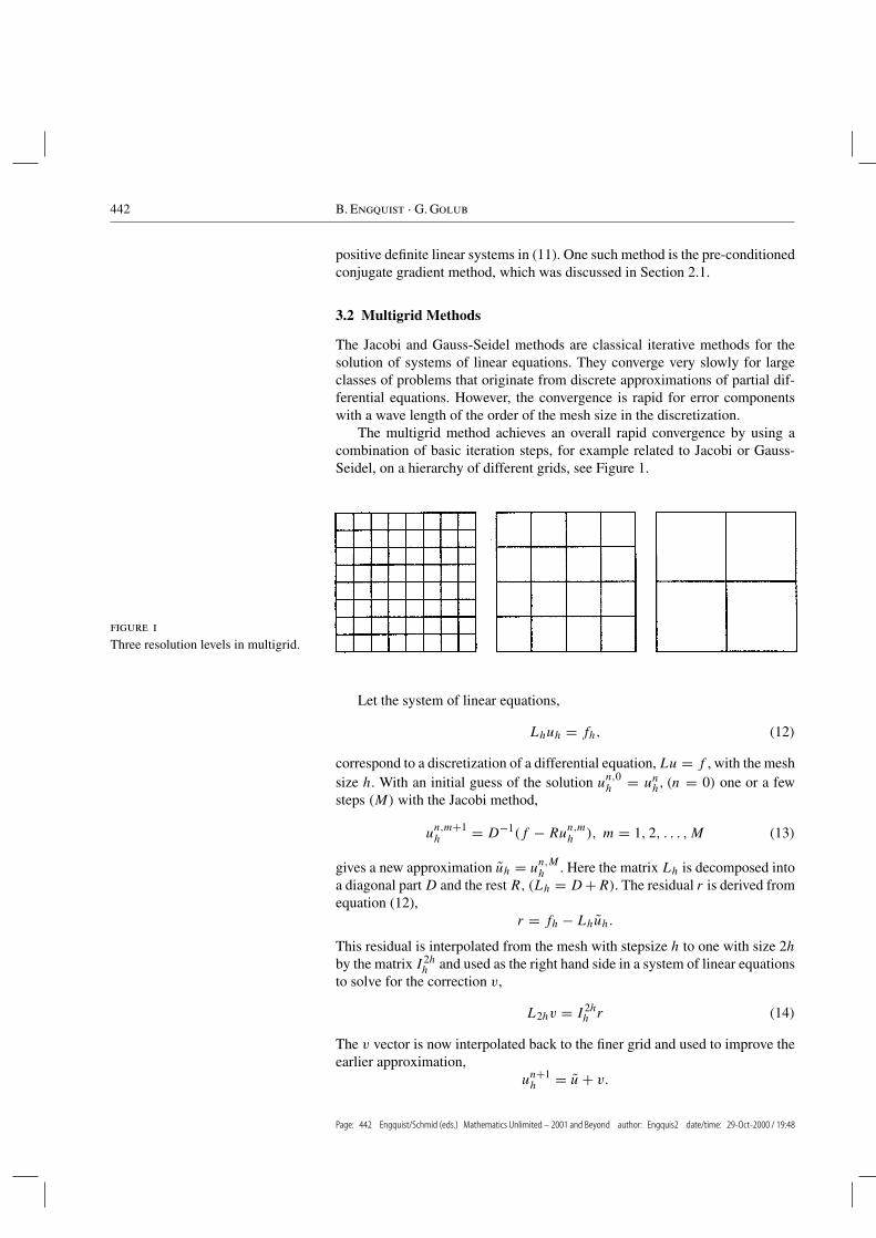
The multigrid method achieves an overall rapid convergence by using acombination of basic iteration steps, for example related to Jacobi or Gauss-Seidel, on a hierarchy of different grids, see Figure 1.
figure 1Three resolution levels in multigrid.
Let the system of linear equations,
Lhuh = fh, (12)
correspond to a discretization of a differential equation,Lu = f , with the meshsize h. With an initial guess of the solution u
n,0h = unh, (n = 0) one or a few
steps (M) with the Jacobi method,
un,m+1h = D−1(f − Ru
n,mh ), m = 1, 2, . . . ,M (13)
gives a new approximation uh = un,Mh . Here the matrix Lh is decomposed into
a diagonal part D and the rest R, (Lh = D+R). The residual r is derived fromequation (12),
r = fh − Lhuh.
This residual is interpolated from the mesh with stepsize h to one with size 2hby the matrix I 2h
h and used as the right hand side in a system of linear equationsto solve for the correction v,
L2hv = I 2hh r (14)
The v vector is now interpolated back to the finer grid and used to improve theearlier approximation,
From Numerical Analysis to Computational Science 443
The procedure can be repeated for n → n + 1 → n + 2 etc. So far this isonly a two-grid method. The full multigrid algorithm results if we again solvethe system (14) by the same procedure and thus involve approximations on ahierarchy of different grids.
The computational complexity for multigrid is optimal for many classes ofproblems. The number of operations required for the solution of a discretizedelliptic problem (12) on the grid in Figure 2 is O (h−2). This is an excellentexample of how much the invention of new algorithms may improve the com-putational cost. Classical Gaussian elimination would need O (h−6) operationsfor the same problem. For large systems (12), which correspond to small h, thegain could be many orders of magnitude.
The algorithm as outlined above can be generalized in many ways. Eventhe notion of grids can be eliminated as is the case in the algebraic multigridmethod and it also applies to the solution of nonlinear equations.
The earliest description of a multigrid method was given by Fedorenko [9]and the initial theory was done by Bakhvalov, [2]. In [3] Brandt demonstratedthe power of these techniques on a variety of problems. For the basic theory seethe classical text by Hackbusch [12].
For many problems today the multigrid method is the most efficient solutiontechnique and it is the standard tool in numerous applications. Multigrid is alsothe first computationally successful example of modern hierarchical methods.Other examples are domain decomposition, the fast multipole method and algo-rithms based on wavelet representations. In multigrid we also use a technique di-rectly adapted to multiscale problems. The different scales (h → 2h → 4h →)
are treated by separate iterations adjusted to the individual scales.
For many problems today themultigrid method is the most ef-ficient solution technique and itis the standard tool in numerousapplications.
3.3 The Singular Value Decomposition
The Singular Value Decomposition (SVD) has been known for many years butits use has become more prominent with the advent of good computational tech-niques. The decomposition has a long history and has often been re-discovered.It is known as the Eckert-Young decomposition in the psychometrics literature.
Let A be an m× n matrix. We assume m ≥ n. Then it can be shown that,
It is easy to show that the non-zero singular value of A are the square roots ofthe non-zero eigenvalues of ATA. Thus,
σi(A) = [λi(AT A)] 12 .
There are a number of interesting problems in matrix approximation thatcan be answered via the SVD. For instance, let A be an m× n matrix of rank r .Now determine a matrix Ak of rank k so that,
‖A− Ak‖2 = min .
The solution is given in a simple fashion:
Ak = UΣkVT ,
where Σk is the same as Σ above, but with σk+1 = · · · = σn = 0. This resultplays an important role in solving ill-posed problems.
The solution of the linear squares problem can be given in terms of the SVD.If we seek the vector x such that,
‖b − Ax‖2 = min and ‖x‖2 = min,
then,
x = A+b,
where A+ represents the pseudo-inverse of A. Then from the SVD of A, wehave,
A+ = VΣ+UT ,
where Σ+ is the n × m diagonal matrix with the reciprocal of the nonzerosingular values. Note that a small singular value can lead to a very large solutionvector x. To regularize the solution some of the small singular values are replacedby zero.
There are many efficient methods for computing the SVD. One of the mostfrequently used techniques is to first bi-diagonalize the matrix A so that,
XTAY =(B
0
),
where XTX = Im and YT Y = In and bij = 0 for i > j and i < j + 1.Then by using a variant of the QR method, the matrixB is diagonalized. The
algorithm is highly efficient and stable and is described in detail in [11]. Thesingular value decomposition has become a useful tool in many applications,and as a theoretical tool, it allows us to understand certain numerical processesmore deeply. It is an algorithm with applications in the traditional scientificfields but also in statistics and data mining, and it is essential in the analysis ofhard ill-posed problems.
The singular value decomposi-tion has become a useful toolin many applications, and asa theoretical tool, it allows usto understand certain numericalprocesses more deeply.
From Numerical Analysis to Computational Science 445
4. Extrapolation in Time – Future Challenges
Interpolation and extrapolation are standard computational techniques that aretaught in all elementary numerical analysis courses. In extrapolation, data rep-resenting a particular function over one domain is used to estimate the functionin another. Most predictions of the future follow simple extrapolation principlesby extending existing trends. The clever choice of exponential extrapolation inMoore’s law has been very successful in predicting the growth of computercapacity. This growth has also been an important driving force for algorithmdevelopment and related analysis.
It is, of course, difficult to predict the innovation of new numerical methodsor new analysis. It is somewhat easier to point to areas where the need fornew development is great. Historically, there has been important progress insuch areas. They contain exciting challenges and often also funding which is arequirement that should not be neglected.
There is a need for new techniques for solving problems where a moderateimprovement in computing power is not enough. These are the computationallyhard problems and the foremost examples are multiscale problems. Ill-posedand inverse problems are other examples.
In multiscale problems the smallest scales must often be resolved over thelength of the largest scales. This results in a very large number of unknowns.Complex interaction between the scales results in complicated equations forthese unknowns. New theories for homogenized or effective equations willbe required, as well as fast numerical algorithms. The methods should be atmost linear in complexity. This means that the number of algebraic operationsshould not grow more than linearly in the number of unknowns. Multigrid issuch an algorithm. It will also be desirable with sub-linear algorithms basedon sampling for very large systems. There are many examples of multiscaleproblems. Turbulence in fluid dynamics is a classical example. Simulation inphysics of any larger segment of scales from elementary particles to galaxiesclearly poses great challenges.
Another area in need of improvements is the user interaction with the com-putational hardware and software. The computation is becoming less expensivebut the cost for a qualified user is not decaying. The amount of data resultingfrom the simulations of tomorrow will be enormous. The development in thisarea will benefit from the general evolution of the fields of visualization, virtualreality, CAD and data mining. Specialized software for computational sciencewill still be needed in order to provide the ideal interactive environment in whichthe scientist can control the computation and easily study multidimensional data.
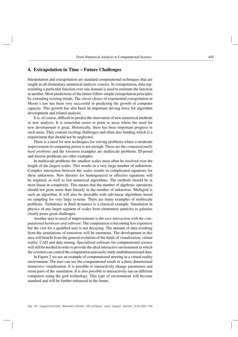
In Figure 2 we see an example of computational steering in a virtual realityenvironment. The user can see the computational result in a three dimensionalimmersive visualization. It is possible to interactively change parameters andrerun parts of the simulation. It is also possible to interactively run on differentcomputers using the grid technology. This type of environment will becomestandard and will be further enhanced in the future.
The user will also require automatically adaptive algorithms with realistica posterior error estimates. This is currently a very active area of research withearly results already in the seventies by Babuska, [1].
In the introduction we mentioned the strong links computational sciencehas to mathematics, the computer and applications. Progress in these fields willdirectly impact the development of computational algorithms.
figure 2Example of computational steering in avirtual reality environment.
The interaction with different branches of mathematics must be strength-ened. The models are becoming more complex and thus deeper mathematicalanalysis is required to understand their properties.
The interaction with differentbranches of mathematics mustbe strengthened.
We have stressed the importance of the increasing computer capability. Ifthere would be a drastic change in the computer architecture, this would imme-diately require substantial modifications of numerical algorithms, in particularin numerical linear algebra. One possible such change could be the introductionof quantum computers.
Fluid and structural mechanics have so far been the most prominent appli-cations influencing the development and analysis of numerical methods. Thiswill change as a broader spectrum of applications will increase in importance.Challenging examples are material science and other branches of fundamentalphysics and chemistry. Simulations in the biological sciences are rapidly becom-ing important tools in research, industrial development and medical practice.The ultimate challenge is a computer model of the human body, which is ascomplete as possible. Social and economical systems are highly complex andpose severe problems for modelling and simulations. Stochastic models will beof importance for these types of systems, which often lack adequate determin-istic descriptions. We are starting to see different interacting processes coupledtogether in the same simulation. This is sometimes called multi-physics com-
From Numerical Analysis to Computational Science 447
putations and it will become even more common in the future. We will alsohave more applications of larger systems for optimization and control whichare based on many algorithms for individual processes.
None of these predictions will come true and none of the challenges willbe met if education fails. Thus, the greatest challenge is the education of newgenerations of computational scientists, who have a thorough understanding ofmathematics, computer science and applications.
Thus, the greatest challenge isthe education of new generationsof computational scientists, whohave a thorough understandingof mathematics, computer sci-ence and applications.
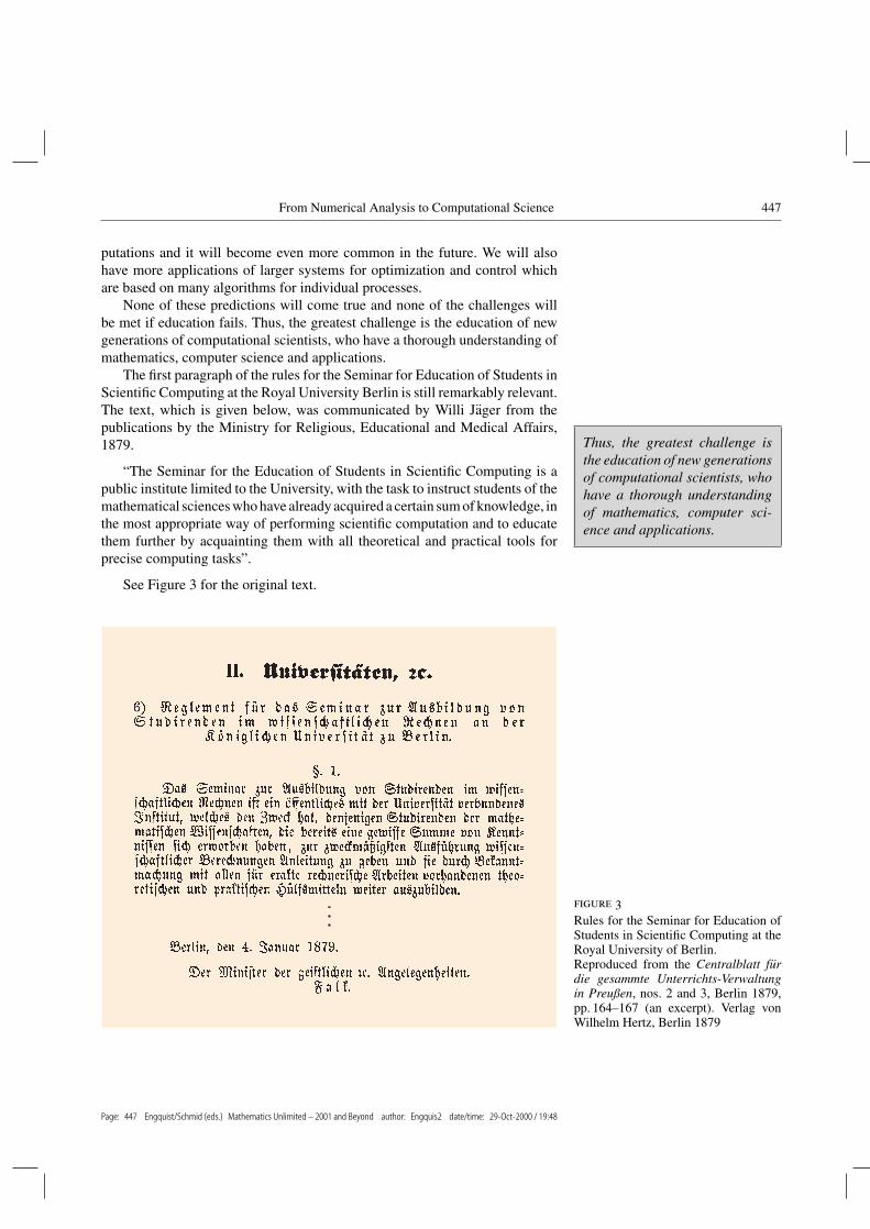
The first paragraph of the rules for the Seminar for Education of Students inScientific Computing at the Royal University Berlin is still remarkably relevant.The text, which is given below, was communicated by Willi Jager from thepublications by the Ministry for Religious, Educational and Medical Affairs,1879.
“The Seminar for the Education of Students in Scientific Computing is apublic institute limited to the University, with the task to instruct students of themathematical sciences who have already acquired a certain sum of knowledge, inthe most appropriate way of performing scientific computation and to educatethem further by acquainting them with all theoretical and practical tools forprecise computing tasks”.
See Figure 3 for the original text.
figure 3Rules for the Seminar for Education ofStudents in Scientific Computing at theRoyal University of Berlin.Reproduced from the Centralblatt furdie gesammte Unterrichts-Verwaltungin Preußen, nos. 2 and 3, Berlin 1879,pp. 164–167 (an excerpt). Verlag vonWilhelm Hertz, Berlin 1879
1. Babuska, I. and W. C. Reinboldt: Error estimates for adaptive finite element com-putations. SIAM J. Numer. Anal. 15 (1978) 736–754
2. Bakhvalov, N. S.: On the convergence of a relaxation method with natural constraintson the elliptic operator. USSR Computational Math. and Math. Phys. 6 (1996) 101–135
3. Brandt, A.: Multilevel adaptive solutions to boundary value problems. Math. Comp.31 (1977) 333–390
5. Chorin, A. J.: A random choice method in gas dynamics. Springer Lecture Notes inPhysics 59 (1976) 129–134
6. Ciarlet, P. G.: The finite element method for elliptic problems. North-Holland, 19787. Dahlquist, G.: Numerical integration of ordinary differential equations. Math. Scand.
4 (1956) 33–508. Dongarra, J. and Sullivan, F.: The top ten algorithms. Computing in Science and
Engineering (2000) 22–799. Fedorenko, R. P.: The speed of convergence of one iterative process, USSR Comput.
Math. and Math. Phys. 1 (1961) 1092–109610. Godunov, S. K.: A difference scheme for numerical computation of discontinuous
solution of hydrodynamic equations. Math. Sbornik 47 (1959) 271–30611. Golub, G. H. and C. Van Loan: Matrix computations. John Hopkins Press, Baltimore
198912. Hackbusch, W.: Multi-grid methods and applications. Springer, Berlin 198513. Nieminen, R. M.: From number crunching to virtual reality: mathematics, physics
and computation. This volume, pp. 937–96014. Osher, S. and J. A. Sethian: Fronts propagating with curvature dependent speed:
algorithms based on Hamilton-Jacobi formulation. J. Comp. Phys. 79 (1988) 12–4915. Richardson, L. F.: Weather predictions by numerical process. Cambridge University
Press, 192216. Richtmyer, R. D., and K.W. Morton: Difference methods for initial-value problems.
John Wiley and Sons, New York 196717. Saad, Y., Iterative methods for sparse linear systems. PWS, New York 199618. Stewart, G.W. and J.-G. Sun: Matrix perturbation theory. Academic Press, New York
199019. Wilkinson, J. H.: The algebraic eigenvalue problem. Clarendon Press, Oxford 196520. Zienkiewicz: The finite element method in engineering science. McGraw-Hill, 1971