From Pressure Maps and Wind Velocityto Northern Lights and Other FascinatingPhenomena on the Rotating EarthCite as: Phys. Teach. 59, 103 (2021); https://doi.org/10.1119/10.0003462Published Online: 11 February 2021
Andrea Gróf
ARTICLES YOU MAY BE INTERESTED IN
Energy CubesThe Physics Teacher 59, 89 (2021); https://doi.org/10.1119/10.0003457
Revisiting Standing Waves on a Circular PathThe Physics Teacher 59, 100 (2021); https://doi.org/10.1119/10.0003461
Surface Currents on the Plates of a Charging CapacitorThe Physics Teacher 59, 86 (2021); https://doi.org/10.1119/10.0003456
applications to atmospheric motions generally take a calcu-lus-based approach.3-5 The use of pressure maps, however, offers a convenient elementary treatment. High school stu-dents are aware that air currents are determined by the dis-tribution of atmospheric pressure, and physics students have presumably seen isobar charts in geography class. Although an isobar chart is the most widely known graphical represen-tation of pressure distribution, it is not easy to interpret the information conveyed by the curves. Before applying pressure maps to learn about wind speed and direction, it is essential to familiarize students with pressure maps. There are a lot of educational websites6 that offer student activities to introduce the pressure gradient force, that is, the force acting on an air parcel owing to pressure difference. In order to proceed, we will need the following result:
If the pressure difference over a small distance x is p, then the force acting on the air contained in a volume V be-tween two surfaces A normal to x is
(1)
The second factor is the pressure gradient that can be read from an isobar chart.
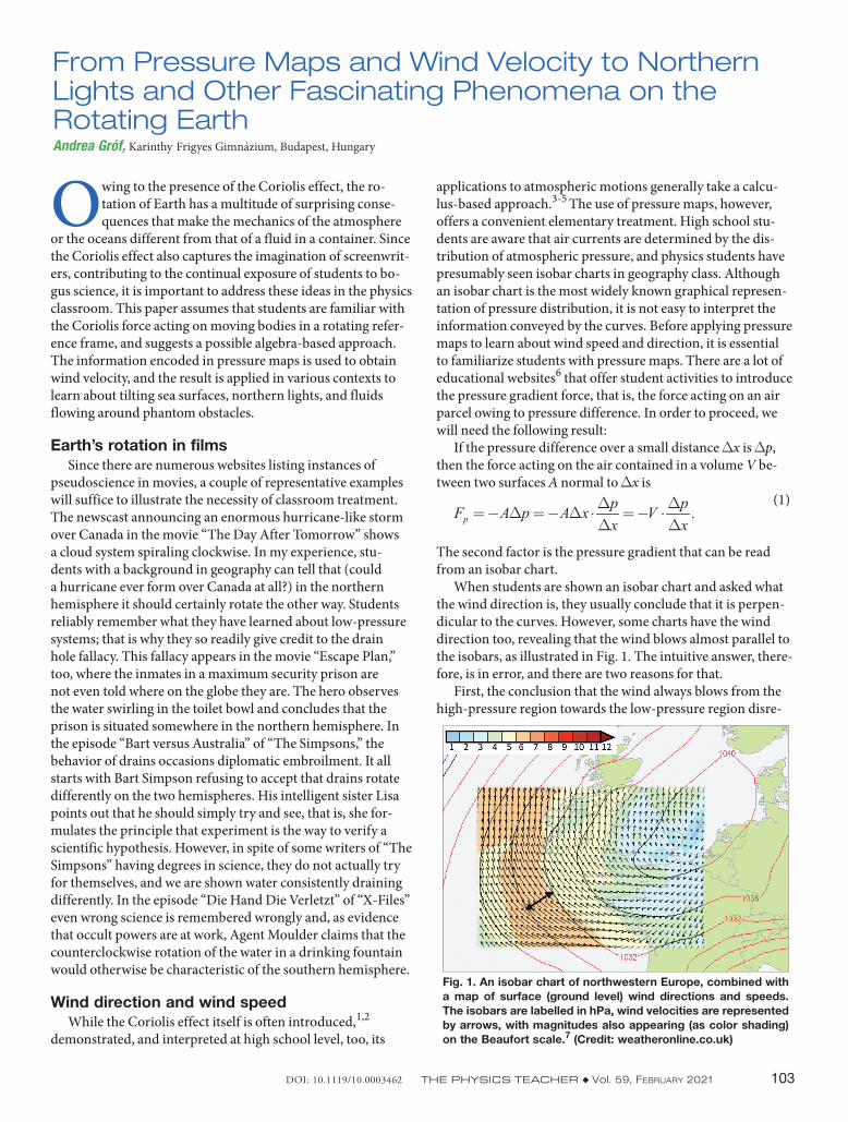
When students are shown an isobar chart and asked what the wind direction is, they usually conclude that it is perpen-dicular to the curves. However, some charts have the wind direction too, revealing that the wind blows almost parallel to the isobars, as illustrated in Fig. 1. The intuitive answer, there-fore, is in error, and there are two reasons for that.
First, the conclusion that the wind always blows from the high-pressure region towards the low-pressure region disre-
From Pressure Maps and Wind Velocity to Northern Lights and Other Fascinating Phenomena on the Rotating EarthAndrea Gróf, Karinthy Frigyes Gimnázium, Budapest, Hungary
Owing to the presence of the Coriolis effect, the ro-tation of Earth has a multitude of surprising conse-quences that make the mechanics of the atmosphere
or the oceans different from that of a fluid in a container. Since the Coriolis effect also captures the imagination of screenwrit-ers, contributing to the continual exposure of students to bo-gus science, it is important to address these ideas in the physics classroom. This paper assumes that students are familiar with the Coriolis force acting on moving bodies in a rotating refer-ence frame, and suggests a possible algebra-based approach. The information encoded in pressure maps is used to obtain wind velocity, and the result is applied in various contexts to learn about tilting sea surfaces, northern lights, and fluids flowing around phantom obstacles.
Earth’s rotation in filmsSince there are numerous websites listing instances of
pseudoscience in movies, a couple of representative examples will suffice to illustrate the necessity of classroom treatment. The newscast announcing an enormous hurricane-like storm over Canada in the movie “The Day After Tomorrow” shows a cloud system spiraling clockwise. In my experience, stu-dents with a background in geography can tell that (could a hurricane ever form over Canada at all?) in the northern hemisphere it should certainly rotate the other way. Students reliably remember what they have learned about low-pressure systems; that is why they so readily give credit to the drain hole fallacy. This fallacy appears in the movie “Escape Plan,” too, where the inmates in a maximum security prison are not even told where on the globe they are. The hero observes the water swirling in the toilet bowl and concludes that the prison is situated somewhere in the northern hemisphere. In the episode “Bart versus Australia” of “The Simpsons,” the behavior of drains occasions diplomatic embroilment. It all starts with Bart Simpson refusing to accept that drains rotate differently on the two hemispheres. His intelligent sister Lisa points out that he should simply try and see, that is, she for-mulates the principle that experiment is the way to verify a scientific hypothesis. However, in spite of some writers of “The Simpsons” having degrees in science, they do not actually try for themselves, and we are shown water consistently draining differently. In the episode “Die Hand Die Verletzt” of “X-Files” even wrong science is remembered wrongly and, as evidence that occult powers are at work, Agent Moulder claims that the counterclockwise rotation of the water in a drinking fountain would otherwise be characteristic of the southern hemisphere.
Wind direction and wind speedWhile the Coriolis effect itself is often introduced,1,2
demonstrated, and interpreted at high school level, too, its
Fig. 1. An isobar chart of northwestern Europe, combined with a map of surface (ground level) wind directions and speeds. The isobars are labelled in hPa, wind velocities are represented by arrows, with magnitudes also appearing (as color shading) on the Beaufort scale.7 (Credit: weatheronline.co.uk)
DOI: 10.1119/10.0003462 THE PHYSICS TEACHER ◆ Vol. 59, February 2021 103
is obtained. Since the Coriolis force acts sideways on a mov-ing object, the pressure gradient force is also sideways, which implies that wind blows along the isobars (called geostrophic wind, in meteorological terms) rather than across them.
Note that this conclusion only applies in the absence of other forces, which is normally the case at high altitudes. The wind velocity vectors representing surface wind in Fig. 1 make an angle with the isobars: at low elevations friction cannot be disregarded, and the equilibrium of forces is as shown9 in the right panel of Fig. 3. Since the pressure gradient force is now greater in magnitude than the Coriolis force, Eq. (2) will only provide a rough upper estimate for the wind speed. In Fig. 1, the thick black double-headed arrow at about 47° latitude marks a distance of approximately 200 km between two iso-bars 4 hPa apart. Substitution in Eq. (2), using an air density of 1.3 kg/m3, delivers a speed of
This would classify as a 7 on the Beaufort scale.7 In reality, Fig. 1 only indicates a level of 6.
The topography of pressure surfacesAlthough the counterintuitive result of wind blowing along
the isobars rather than across them is remarkable enough, by investigating pressure distribution in a little more depth we can also explain some further unexpected behavior of the atmosphere and the seas. Students are not likely to be aware
that isobars are only used in ground level pressure charts. The maps representing upper level pressure distributions are dif-ferent: they show lines of constant altitude for some specific isobaric surface. Meteorologists call these curves isohypses.10 Figure 4 is a 500-hPa isohypse chart, that is, it can be inter-preted as a chart showing the topographic contour lines of the surface enclosing the lower half of the atmospheric air.
In order to see why these curves are more helpful than iso-bars, consider the acceleration owing to the pressure gradient force (1), transformed a little further:
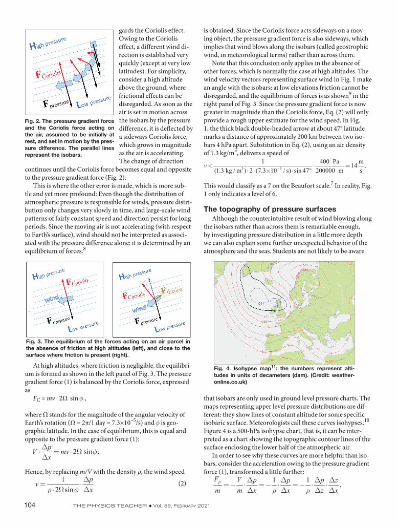
gards the Coriolis effect. Owing to the Coriolis effect, a different wind di-rection is established very quickly (except at very low latitudes). For simplicity, consider a high altitude above the ground, where frictional effects can be disregarded. As soon as the air is set in motion across the isobars by the pressure difference, it is deflected by a sideways Coriolis force, which grows in magnitude as the air is accelerating. The change of direction
continues until the Coriolis force becomes equal and opposite to the pressure gradient force (Fig. 2).
This is where the other error is made, which is more sub-tle and yet more profound: Even though the distribution of atmospheric pressure is responsible for winds, pressure distri-bution only changes very slowly in time, and large-scale wind patterns of fairly constant speed and direction persist for long periods. Since the moving air is not accelerating (with respect to Earth’s surface), wind should not be interpreted as associ-ated with the pressure difference alone: it is determined by an equilibrium of forces.8
At high altitudes, where friction is negligible, the equilibri-um is formed as shown in the left panel of Fig. 3. The pressure gradient force (1) is balanced by the Coriolis force, expressed as
FC = mv . 2Ω sin ,
where Ω stands for the magnitude of the angular velocity of Earth’s rotation (Ω = 2π/1 day = 7.3×10⁻⁵/s) and is geo-graphic latitude. In the case of equilibrium, this is equal and opposite to the pressure gradient force (1):
Hence, by replacing m/V with the density ρ, the wind speed (2)
Fig. 2. The pressure gradient force and the Coriolis force acting on the air, assumed to be initially at rest, and set in motion by the pres-sure difference. The parallel lines represent the isobars.
Fig. 3. The equilibrium of the forces acting on an air parcel in the absence of friction at high altitudes (left), and close to the surface where friction is present (right).
Fig. 4. Isohypse map11: the numbers represent alti-tudes in units of decameters (dam). (Credit: weather-online.co.uk)
104 THE PHYSICS TEACHER ◆ Vol. 59, February 2021
in the case of the sea there exists a natural isobaric surface: that of the sea level where the pressure equals the atmospheric pressure. The expression (3) thus implies that a current in dy-namic equilibrium involves a tilted surface. This is indeed the case with the Gulf Stream, a current that everyone is familiar with since it even features in the popular media, in the context of climate change scenarios.
For example, consider the section of the Gulf Stream where it flows towards the northeast at 36° northern latitude. The width of the stream is in the order of 100 km, and it flows at a rate of about 1 m/s. These data provide an order-of-mag-nitude estimate for the tilt of the sea surface across the Gulf Stream. The numerical value of the slope expressed from (3) is
where z stands for altitude. Students know from basic fluid mechanics that the pressure at a depth h in a lake is p = p0 + rgh, where p0 is the pressure at the surface. To gener-alize, we can observe that pressure decreases with altitude at a rate proportional to the density of the fluid. Density may vary with position, but in this way density will cancel out of the equation, leaving only the known value of g and the slope of the isobaric surface:
Under equilibrium conditions, this acceleration, expressed in terms of the slope of the isobaric surface, can again be set equal to the Coriolis acceleration, to yield a new expression for the speed:
(3)
For example, consider the region of the English Channel in Fig. 4. z = 240 m can be read from the contour lines and
x can be measured on a geographic map (about 660 km). We can use 51° for latitude. Figure 5 shows the region magnified, also indicating wind direction and the necessary geographic information.
With these data, the wind speed at a height of about 6 km (where g = 9.8 ms–2 is still applicable) above the English Channel is
Ω
Figure 6 shows a streamline map of actual wind velocities at 500 hPa height over the same region, a few hours earlier. Observe that at this high altitude the direction of the wind is, indeed, along the curves.
Where sea level is not levelNote that velocity depends (on geographic latitude and)
on the slope of the pressure surfaces. This is a conclusion that lends itself to further discussion. One interesting consequence is obtained if the result (3) is applied to the oceans. Evidently,
Fig. 5. Isohypse map with geographic data and wind direction.
Fig. 7. Map of sea surface topography obtained from satellite measurements, also showing fluid velocities represented by the black lines. The Gulf Stream is the narrow band separating the blue and light red regions. Observe the eddies accompanying the stream, and the depression of the surface inside the great counterclockwise eddy near the middle of the figure. (Credit: Gerald Dibarboure)
THE PHYSICS TEACHER ◆ Vol. 59, February 2021 105
be observed in nature, too: Polar lights often exhibit shapes13
resembling the fluid curtains of Fig. 8, and it is possible to ex-plain the formation of the curtain-like displays analogously.14
Polar lights are emitted in the upper atmosphere by air molecules excited by the charged particles that precipitate from the solar wind into the terrestrial atmosphere, along the lines of magnetic field. If density is uniform, the rate of pressure decrease with height, –ρg, is the same at all altitudes; therefore z/ x is the same at all altitudes, and the velocity of gas molecules situated along a vertical line is also independent of the altitude. The molecules will thus all move identically, that is, along identical trajectories, forming curtain-like struc-tures, as illustrated in Fig. 9. It is these curtain-like shapes that become visible if the gases are made to glow owing to excitation.
For a natural Taylor column, the most frequently cited example is the photograph in Fig. 10, showing the behavior of clouds over the Pacific island of Guadalupe. The clouds are a lot higher than the island, but the well-known pattern of the von Kármán vortex street reveals that the wind flows around the stationary air column over the island, as if it had hit an obstacle.
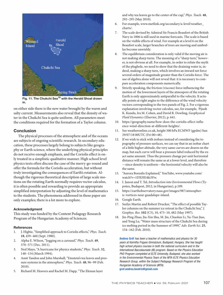
The example of the summer ice retreat on the Chukchi Sea is not so widely known, but no less instructive. The Chuk-chi Sea lies to the north of the Bering Strait, bounded by the coasts of Alaska and Siberia (and by the rim of the continental shelf on the north). The Herald Shoal rises about 20 meters above the seabed that has a roughly uniform depth of 50 me-ters (Fig. 11).
In summer, a warm current arriving from the Bering Strait regularly melts the ice cover of the Chukchi Sea. Research17,18 revealed that the ice retreat follows the same pattern year by year. Actually, even ship logs of 19th-century whalers contain the observation that warm water advances like a tongue on each side of the Herald Shoal, and when the ice has melted at the sides and even beyond the shoal, there is still an ice cover over the shoal itself, for a long time. Temperature measure-ments show a well-defined front at the edge of the shoal, and so do measurements of salinity. Under the persisting ice cover over the shoal, there is colder and less saline old water, while
That means a rise of about 1 m over a distance of 100 km northwest to southeast: in good agreement with values ob-tained by satellite altimetry, as represented in Fig. 7.
Fluid curtains and phantom columnsAnother interesting consequence follows when density
can be considered uniform in a fluid (be that air or water). In that case pressure decreases with height at the same rate, –ρg, along a vertical line erected at any point of the surface. Thus pressure surfaces have the same slope all along the vertical line, which results in the same horizontal velocity all along the vertical line.12
It should be borne in mind that this con-clusion only applies to fluids of uniform density that rotate fast enough for the Coriolis force to be important. The in-variance of rotated fluids under vertical translation can also be demonstrated in the laboratory. The picture of Fig. 8 shows a water tank placed on a rotating platform in the von
Kármán Laboratory for Environmental Flows at ELTE Uni-versity, Budapest. In the rotating water, a drop of dye has been injected. The same dye injected in a stationary tank would form a cloud showing turbulence in all three dimensions. Rotation, however, makes a great difference: the dye spreads along vertical surfaces resembling curtains.
Figure 8 demonstrates more than that: the most surprising behavior of a rotating fluid is observed if an obstacle is placed at the bottom of the tank. Although the obstacle is much
lower than the water level in the tank, the dye will not flow over the obstacle. The dye curtains not only flow around it at the bottom where the true obstacle is but also flow around an imagi-nary column over the obstacle.
Fluid curtains and the column remaining at rest over an obstacle (a so-called Taylor column) can both
Fig. 8. Dye curtains in a rotating water tank. Demonstration in the von Kármán Laboratory for Environmental Flows.
Fig. 9. When density is uniform, curtain-like shapes of polar lights result from the invari-ance of the flow under a vertical transla-tion.
Fig. 10. Kármán vortex street over the island of Guadalupe.15 (Credit: NASA/GSFC/JPL, MISR Team)
106 THE PHYSICS TEACHER ◆ Vol. 59, February 2021
and why tea leaves go to the center of the cup,” Phys. Teach. 48, 292−295 (May 2010).
6. For example, www.metlink.org/secondary/a-level/weather_charts/.
7. The scale devised by Admiral Sir Francis Beaufort of the British Navy in 1806 is still used in marine forecasts. The scale is based on the visible effects of wind. For example at a level 6 on the Beaufort scale, larger branches of trees are moving and umbrel-las become unwieldy.
8. The equilibrium consideration is only valid if the moving air is not making sharp turns. The meaning of a “sharp turn,” howev-er, is not obvious at all. For example, in order to refute the myth of the plughole, we need to show that the draining water is, in-deed, making a sharp turn, which involves an inward net force several orders of magnitude greater than the Coriolis force. The use of algebra alone will not reveal that: it is necessary to com-pare acceleration components numerically.
9. Strictly speaking, the friction (viscous) force influencing the motion of the lowermost layers of the atmospere of the rotating Earth is only approximately antiparallel to the velocity. It actu-ally points at right angles to the difference of the wind velocity vectors corresponding to the two panels of Fig. 2. For a rigorous explanation involving vector calculus, see, for example, Pijush K. Kundu, Ira M. Cohen, and David R. Dowling, Geophysical Fluid Dynamics (Elsevier, 2012), p. 641.
11. See weatheronline.co.uk, height 500 hPa ECMWF (gpdm) Sun 29/07/18 00UTC (Fri 00+48).
12. If we wish to stick with isobars instead of considering the to-pography of pressure surfaces, we can say that in an isobar chart of a little higher altitude, the very same curves are drawn on the map, but each curve will bear a pressure label reduced by the ex-act same amount. Thus the pressure change per unit horizontal distance will remain the same as at a lower level, and therefore —since density is uniform—the horizontal velocity will also be the same.
16. Google Earth.17. Seelye Martin and Robert Drucker, “The effect of possible Tay-
lor columns on the summer ice retreat in the Chukchi Sea,” J. Geophys. Res. 102 (C5), 10, 473−10, 482 (May 1997).
18. Jin-Ping Zhao, Jiu-Xin Shu, M. Jin, Chaolun Li, Yu-Tian Jiao, and Yong Lu, “Water mass structure of the Chukchi Sea during ice melting period in the Summer of 1999,” Adv. Earth Sci. 25, 154−162 (Feb. 2010).
Andrea Gróf has been a teacher of mathematics and physics for 30 years at Karinthy Frigyes Gimnázium, Budapest, Hungary. She has taught high school physics courses in both the national curriculum and in the International Baccalaureate (IB) program. Based on the Physics Education PhD Program completed at ELTE University, Budapest, she also worked in the Environmental Physics Team of the MTA-ELTE Physics Education Research Group, within the Subject Pedagogy Research Program of the Hungarian Academy of Sciences (MTA)[email protected]
on either side there is the new water brought by the warm and salty current. Measurements also reveal that the density of wa-ter in the Chukchi Sea is quite uniform. All parameters meet the conditions required for the formation of a Taylor column.
ConclusionThe physical processes of the atmosphere and of the oceans
are subjects of ongoing scientific research. In secondary edu-cation, these processes largely belong to subjects like geogra-phy or Earth science, where the underlying physical principles do not receive enough emphasis, and the Coriolis effect is on-ly treated in a simplistic qualitative manner. High school level physics texts often discuss the case of the merry-go-round and offer the formula for the Coriolis acceleration, but without truly investigating the consequences of Earth’s rotation. Al-though the rigorous theoretical description of large scale mo-tions on the rotating Earth normally requires vector calculus, it is often possible and rewarding to provide an appropriate simplified interpretation by adjusting the level of mathematics to the students. The phenomena addressed in these paper are only examples; there is a lot more to explore.
AcknowledgmentThis study was funded by the Content Pedagogy Research Program of the Hungarian Academy of Sciences.
References1. J. Higbie, “Simplified approach to Coriolis effects,” Phys. Teach.
18, 459−460 (Sept. 1980).2. Alpha E. Wilson, “Jogging on a carousel,” Phys. Teach. 49,
570−571 (Dec. 2011).3. Ned Mayo, “A hurricane for physics students,” Phys. Teach. 32,
148−154 (March 1994).4. Amit Tandon and John Marshall, “Einstein’s tea leaves and pres-
sure systems in the atmosphere,” Phys. Teach. 48, 96−99 (Feb. 2010).
5. Richard M. Heavers and Rachel M. Dapp, “The Ekman layer
Fig. 11. The Chukchi Sea16 with the Herald Shoal drawn in.