From Sweden to America:

Migrant Selection and Social Mobility During the Era of Mass Migration

Martin Dribe1, Björn Eriksson1 and Jonas Helgertz1,2

1. Centre for Economic Demography and Department of Economic History, Lund University

2. Minnesota Population Center, University of Minnesota

Martin.Dribe@ekh.lu.se, Bjorn.Eriksson@ekh.lu.se, Jonas.Helgertz@ekh.lu.se

This is a first draft of the proposed paper. In the final version we will also study social

mobility of Swedish migrants to the U.S. by linking the data to the U.S. full count censuses of

1900, 1910 and 1920. In the analysis the social mobility of migrants in the U.S. labor market

will be compared with similar stayers in Sweden using parish-of-origin and sibling fixed-

effects models. These comparisons will provide a good picture of individual-level

probabilities of social mobility related to long-range migration.

Introduction

Between 1850 and 1930 over 30 million people left Europe for North America, with the vast

majority ending up in the United States. Sweden was one of the most important sending

countries together with Ireland, Britain, Norway, Italy, Portugal and Spain (Baines 1991). In

total 1.1 million Swedes left for the United States during the whole period 1850-1930, and an

additional 20,000 left for Canada (Carlsson 1976). In 1900, Sweden had a population of about

5 million. About 18 percent of the emigrants returned to Sweden in the period 1875-1930

(Tedebrand 1976). The enormous scale of this flow of people across the Atlantic has triggered

a large body of research trying to understand why people left, how they fared in the new

country, and the impact of this flow on sending and receiving countries. This issue is of great

relevance not only to fully understand an important historical process, but also to gain better

knowledge about migration in contemporary societies; who moves, what factors are important

for immigrant integration in host societies, and what impact does large scale migration have

on sending and receiving countries. These questions are at the forefront of the policy

discussion in most Western societies of the early 21st century (see Abramitzky and Boustan

2017).

While there has been a great deal of research on mass migration across the Atlantic,

there has not been much research based on individual-level data analyzing the selection of

migrants. Instead, most research has either been based on qualitative accounts or aggregate

quantitative data focusing on the describing and explaining the migration process from a

regional or even country perspective (e.g. Hatton and Williamson 1994; Hatton 2010, for

Sweden, see e.g. Thomas 1941; Norström 1988; Runblom and Norman 1976). More recently,

there has been some efforts to look at migration selection also from an individual perspective,

most notably the work on Norway by Abramitzky et al. (2012, 2013).

The aim of this paper is to contribute to this line of research by studying the selection

mechanisms of migration from Sweden to the United States during the age of mass migration.

Were migrants positively or negatively selected on occupational status and social origin

(occupation of fathers)? Did the selection differ by gender, urbanicity and region as has

sometimes been argued in the literature? These questions are important to increase our

understanding of the forces behind the mass migration, but as pointed out by Abramitzky and

Boustan (2017), they it is also crucial to have a solid knowledge of selection mechanisms to

correctly assess the assimilation of immigrants into host societies.

We link individuals across the Swedish censuses 1880, 1890, 1900 and 1910 as well

as to emigration lists. The censuses provide information on occupation, household, and family

context as well as place of residence, and the migration registers give date of migration to the

United States. We use an occupation-based class scheme (HISCLASS) to measure of social

class and data on GDP/capita in both Sweden and the United States as a measure of

macroeconomic push and pull factors. Moreover, we look at selection patterns by region,

urban/rural, and over time to better understand the determinants of migration in this era.

Lastly, the ability to link individuals back to their childhood home allows for the estimation of

sibling fixed-effect models, cancelling out the influence of unobserved background

characteristics on the propensity to migrate.

Our findings suggest that migrants were disproportionally drawn from the working

class, and especially the skilled workers. White-collar workers were least prone to emigrate to

the United States, regardless of region, time period or detailed model specification. Overall,

farmers were less likely to emigrate as were farmer sons and daughters, but the pattern

differed by region and also changed over time. Similarly, the relative migration propensity of

unskilled workers depended on region and changed over time. All classes were similarly

affected by the economic push and pull factors, with a somewhat stronger response to the US

pull from the most migration prone groups. Selection patterns were similar for men and

women and for rural and urban areas, but differed in important ways across regions and over

time.

Background

Swedish emigration to the United States took off in earnest in the 1860s and peaked in the

1880s before gradually falling before the First World War, with a total around 1.1 million

Swedes crossing the Atlantic (see Figure 1). Long-range migration flows are typically

analyzed and understood as the result of economic differences between sending and receiving

regions. Within this paradigm, individuals from regions with a large endowment of labor

relative to capital migrate to destinations with higher wages and relatively lower endowments

of labor in order to improve their economic conditions, a process which continues until an

equilibrium state between the source and destination is met (Barro and Sala-i-Martin 1991;

Harris and Todaro 1970; Hatton and Williamson 1998). Empirically, basic economic

differences have been shown to be an important explanation for historical migration flows

from peripheral rural regions, with plentiful labor and low wages, to cities and industrializing

regions where labor was in demand and wages accordingly higher (Boyer 1997; Boyer and

Hatton 1997; Grant 2000; Bohlin and Eurenius 2010). As a consequence, emigration from

Europe to the United States eroded economic differences and drove wages to convergence

between countries in the 18th century (Taylor and Williamson 1997).

Economic conditions are not stable in the short and medium term, which creates

economic fluctuations in both sending and receiving countries. These fluctuations constitute

short-term push and pull factors creating cycles also in migration, which are evident for

Sweden in Figure 1 (e.g., Thomas 1941; Quigley 1972; Wilkinson 1967; see also Hatton

2010). The most important aspects of short-term economic fluctuations may not have been in

wages but in job opportunities linked business cycles in industry or agriculture (Gould 1979).

Figure 1 here

From an individual perspective, emigration may be conceptualized as a decision that

involves a cost-benefit analysis based on anticipated earnings, costs and other benefits. If the

net expected return from moving is positive, migration subsequently takes place (Sjastaad

1962; Todaro 1969). Economic conditions in the origin and destination must thus be

considered together with individual characteristics and intervening obstacles which also form

part of the decision process and affect the probability of migration and the destination choice

(Lee 1966; Harris and Todaro 1970). By moving to a location with better prospects for

upward occupational mobility or higher wages, anticipated earnings increase as a result

(Sjaastad 1962; Long 2005; Borjas 1994). These gains are weighed against costs, which,

particularly in the 18th and early 19th centuries, were primarily determined by migration

distance. The distance between two locations is a proxy for both monetary costs associated

with a particular move, uncertainty regarding conditions in the destination and the

psychological cost implied by the separation from amenities in the origin such as friends and

family (Sjaastad 1962; Schwartz 1973).

There are a number of factors which mediate the effect of distance. At the regional

level, access to transportation and communication infrastructure such as roads, railways and

postal services lowers travel and communication costs (Keeling 1999). Networks, defined as a

community of family and friends (kinship networks), or migrants from the same origin

(migrant network), can help to lower the migration costs (e.g. Wegge 1998). In particular,

psychological, information, job-search, and housing costs will be lower for individuals with

large networks, as previously settled migrants help more recent ones navigate life in the

destination.

The theoretical framework outlined above provides as useful starting point when

considering emigration from Sweden to the United States during the age of mass migration.

First it is important to point out that the US border in effect was open in this period, which

allows a study of migrant selection without the problematic legal concerns that affects

assessments of selection mechanisms in most contemporary contexts (Abramitzky and

Boustan 2017). In the 1860s a series of poor harvests in Sweden served as a push factor that

resulted in the first wave of emigration that quickly receded before picking up again in the

late 1870s and peaking in the 1880s (e.g. Carlsson 1976). During the 1880s import of cheap

grain from America and Russia led to falling grain prices and economic difficulties for many

farmers, which constituted a push factor in the emigration peak 1887-1888, before the

introduction of import tariffs on grain in 1888 (Schön 2010: 195-201; Carlsson 1976). Better

economic conditions in Sweden, economic crisis in the United States in the second half of the

1890s contributed to a decline in emigration in this period, but it was followed by a new peak

in the early years of the 1900s.

The transformation of the rural sector in the period of mass migration would lead us

to expect migrants to have been disproportionally drawn from the agricultural groups of

farmers and rural laborers, which is also confirmed by the aggregate statistics (cf. Carlsson

1976).

Throughout the period of mass migration, cheaper and safer forms of transportation

together with a growing expatriate community also made migration more affordable and

accessible. Simultaneously, in particular after 1880, rapid economic growth in Sweden meant

convergence relative to the United States. On the eve of World War I, the closing of the

American frontier and Sweden’s robust economic performance had eroded many of the

incentives that had attracted emigrants over the past 50 years. Still, emigration continued after

the war before diminishing in the late 1920s just before the depression (Carlsson 1976). Even

though emigration from Sweden to the United States did not completely stop, the era of mass

migration was definitely over by 1930.

Differences in economic conditions between Sweden and the United States did not

only affected the number of emigrants, but also determined who were able and willing to

move. Expectations, ability, benefits, costs and resources are all characteristics that vary

between individuals and simultaneously determine the returns to migration and the incidence

thereof. As a result, migration is a highly endogenous process undertaken by a certain groups

and individuals, each differently selected depending on individual characteristics and

circumstances. If costs are important, we expect migrants to be selected among the most able,

ambitious and entrepreneurial individuals who expect to be able to recoup costs in the form of

substantial returns (Lee 1966). Similarly, costs may affect selection if costs are a negative

function of ability, the able being “more efficient in migration” (Chiswick 1999). Upfront

costs also act as a more direct barrier by preventing the financially constrained from moving.

Even when costs are fixed, as in the case of a train or boat ticket, migration is still relatively

more expensive for the less skilled because fewer hours of work are required on the part of the

more able to cover expenses associated with a move.

Although migrants tend to be younger, the relationship between age and the

probability of migration is not straightforward. Becker (1964) argues that the propensity to

migrate decreases with age, because the net present value of benefits is higher for younger

prospective migrants due to greater duration of stay in a particular destination. Older workers

may also be less mobile the costs of liquidating physical and personal investments in the

origin is higher (Schwartz 1976). However, migration costs may be more affordable for older

prospective migrants than younger ones due to higher earnings and accumulated assets.

In a series of articles building on Roy (1951), Borjas (1987) shows how migrant

selection depends on differences in individual ability and returns to skills between locations.

The model’s point of departure is an initial mismatch between ability and the return to skills

in the place of origin. This mismatch is resolved through migration. In order to improve their

lot, high-ability individuals will move from countries with low returns to skills to countries

with high returns to skills, while low-ability individuals will move in the opposite direction.

As a result, migrant selection is driven by an interaction between economic conditions and

individual characteristics. The returns to skills are related to the level of income inequality in

the sending and receiving countries. Higher income inequality implies a higher return to

skills, and hence, the model predicts a negative selection on skills when the sending countries

have greater income inequality than receiving countries, while the selection will be positive in

terms of skills when the receiving country has greater income inequality than the sending

country. There is some discussion in the literature if it is absolute or relative differences in

income that are the most important (see Abramitzky and Boustan 2017). Research on the

transatlantic migration of the nineteenth century seems largely consistent with the Roy model

(e.g. Stolz and Baten 2012). Immigrants from Germany and England seem to have come from

the lower middle class or artisans and farmers, rather than from the poorest working class.

Immigrants from the peripheral countries, with greater inequality than the United States at the

time, were more negatively selected (Wegge 2002; Abramitzky and Boustan 2017). There

were, however, also important differences within countries, for example between rural and

urban areas (Abramitzky et al. 2012) and richer and poorer regions (Spitzer and Zimran

2018).

According to previous research on income inequality around the turn of the 20th

century, Sweden appears as slightly more unequal than the United States in terms of income.

Looking at the share of income earned by the top 1% it was about 20-25% in Sweden 1900-

1910, while it was below 20 in the United States in 1913 (Roine and Waldenström 2008,

2015: 494). Assuming that these differences reflect differences in returns to skills, we would

expect Swedish migrants to have been negatively selected on skills. We would thus expect

unskilled to be most migration prone, and highly skilled least migration prone.

Taken together, we expect migrants to have been selected among the less skilled, and

especially from the rural sector. We also expect economic fluctuations to have affected the

selection of migrants, and also that selection changed over time as well as differed across

regions.

Data and methods

Concerted efforts to digitalize complete censuses have made detailed individual-level data

available for the complete Swedish population in the decades around 1900 (1880, 1890, 1900,

and 1910). The census data have been digitized by the Swedish National Archives and are

published by the North Atlantic Population Project (NAPP, www.nappdata.org), which adopts

the same format as the Integrated Public Use Microdata Series (IPUMS). The Swedish

historical censuses differ from the US and British ones in that they were not done by

enumerators but instead the result of excerpts from continuous parish registers kept by the

Swedish Lutheran Church. Therefore, Swedish censuses do not suffer from quality issues

such as misreporting of age or birthplace which is common in other historical records. A final

unique feature of the Swedish historical censuses is that women consistently appear with their

maiden name recorded, even after marriage. This enables us to link women between sources

to nearly the same extent as men. To identify emigrants, we complement the censuses with

Swedish emigration registers which enables us to accurately identify emigrants (Emibas

2005).

To turn the cross-sectional population registers into panel data, the same individual

needs to be identified at various points in time in the sources. Unlike modern databases,

historical population registers do not contain any personal identification numbers.

Identification of individuals between the sources must therefore rely on matching based on

individual characteristics such as birth place, birth year, sex and names. As a result, we

employ methods which provide an objective measurement of the degree of similarity of

observations obtained from two separate sources of data (see Eriksson 2015; Feigenbaum

2016). The final result is a very large longitudinal data set which allows us to follow

individuals which remained in Sweden or emigrated to the United States between 1880 and

1920. The emigration registers allow for the precise identification of emigrants to the United

States, a substantial improvement on previous studies which have inferred emigration by

locating individuals with similar characteristics in different time periods in the sending

country and US censuses (e.g. Abramitzky et al. 2012).

We link each census to the next subsequent census and to the emigration registers for

the ten-year period following the census. For example, the 1880 census is linked to the 1890

census, and to emigrants in the emigration register departing Sweden between 1881 and 1890.

To deal with multiple emigration events, we identify multiple observations of the same

individual in the emigration registers and only consider the earliest departure when linking to

the censuses.

To avoid introducing bias, only time-invariant variables are used in matching

individuals between the sources: birth year, birth place, sex, and names (see Ruggles, 2006).

Birth year, sex, and birth place do not suffer from the problems of variation in spelling

associated with names and are therefore used to index the data. In practice, this means that

individuals are only compared to potential matches between censuses if the birth year, birth

parish and sex match exactly between the sources. Names (first names and surnames) are

matched using probabilistic linking. Prior to linking, names were subjected to some very

limited and basic standardization. To reduce the homogeneity of patronymic and noble

surnames, the suffixes -sson and -sdotter was parsed out and nobility particles (e.g., von and

af) were eliminated from the surname string. In the Swedish censuses children residing with

their parents rarely have a recorded surname. We deal with this problem by appending both

their father’s surname and a constructed patronymic surname based on the father’s first name.

An individual can thus be linked based on either the similarity of a recorded surname, or in

cases where no surname is recorded, the similarity of inferred family names or a patronymic

name. We evaluate the similarity of names using the Jaro-Winkler algorithm. The algorithm

produces a similarity score (ranging from 0 for completely dissimilar records to 1 for identical

records) by considering common characters, transpositions, and common character pairs. The

score increases if a string has the same initial characters, and it checks for more agreement

between long strings than between short ones and adjusts the score accordingly.

We apply a threshold which the Jaro-Winkler score must exceed for a link to be

considered true. We use individuals with multiple first and surnames to calibrate the

threshold. By plotting different threshold values against the share of links which we can

confirm as true based on the comparisons of names not used in the matching process itself we

are able to evaluate different threshold values in terms of both linkage rates and quality. We

find that beyond a Jaro-Winkler threshold of 0.85, the share of individuals that could be

confirmed when evaluating multiple names does not improve (see Eriksson 2015). Higher

thresholds do, however, result in lower linkage rates. To maximize the number of links while

simultaneously minimizing false positive links, a Jaro-Winkler threshold of 0.85 for

classifying a link as true is chosen. After creating an initial sample of primary links and

removing all ambiguous matches, an additional sample of secondary links is created from the

remaining unlinked pool of individuals by exploiting the indirect linking of households

created by primary links in the first stage.

The linkage rate between the sources is high; on average we link more than two

thirds of individuals between the censuses and to the emigration register. The analytical

capacity of these data sets has been demonstrated in Dribe et al. (2017), Dribe and Eriksson

(2018) and Eriksson et al. (2017). Importantly, the number of linked emigrants in every year

almost exactly mirror the aggregate flows of migrants from Sweden to the United States

between 1880 and 1920 (see figure 2).

Figure 2 here

In the empirical analysis we use two different analytical samples. Throughout, we

select men and women aged 20-44 at the time of the census. These ages are the most

important when it comes to examining emigration from Sweden during this period (e.g.

Carlsson 1976). When addressing the role of individual level characteristics, we rely on a

cross sectional data setup, where individuals in the four censuses are linked to the emigration

lists for the subsequent ten-year period (having emigrated to the United States). Consequently,

individuals observed in the 1880 census are at risk of emigrating between 1881-1890, whereas

those observed in the 1890 census are linked to emigration records between 1891-1900, and

so forth.

We study migrant selection in terms of occupational class attainment. Occupations in

the censuses have been coded in HISCO, an international comparative coding scheme for

occupations (Van Leeuwen et al., 2002). Based on HISCO social classes can be measured

using HISCLASS (Van Leeuwen and Maas, 2011), which is a 12-category classification

scheme based on skill level and degree of supervision, whether manual or non- manual and

whether urban or rural. It contains the following classes: 1) higher managers, 2) higher

professionals, 3) lower managers, 4) lower professionals and clerical and sales personnel, 5)

lower clerical and sales personnel, 6) foremen, 7) medium-skilled workers, 8) farmers and

fishermen, 9) lower-skilled workers, 10) lower-skilled farm workers, 11) unskilled workers,

and 12) unskilled farm workers. In order to make the results more easily interpretable, we

have grouped the HISCLASS categories into four groups (not counting those with a missing

observation on occupation): White-collar workers (HISCLASS 1-5), Skilled workers

(HISCLASS 6-7); Farmers and fishermen (HC8), and Unskilled workers (HISCLASS 9-12).

The white-collar group is quite heterogeneous but is still expected to have higher skills and

more education on average than the other groups, as well as higher earnings and social

prestige (especially the top groups of the white-collar workers). Farmers are distinctive due to

their strong connection to land and property, while the unskilled workers were at the bottom

of the social ladder, in terms of skills, education and earnings, as well as overall social

prestige.

In the analysis, we control for a range of individual and contextual factors. At the

individual level, we account for living in the parental home, region, place of residence

(rural/urban), marital status, migration history, and religion (Lutheran/other religion). At the

contextual level, we include number of variables at the parish level which are assumed to be

important for the migration decision. We expect the share of same-sex individuals to have a

positive effect on the propensity to migrate, as it, for example, should have implications for

the marriage market to which the individual has access. It is known that migration to a

considerable extent is a group phenomenon, where being acquainted with individuals who

either have already or have decided to emigrate will lower the experienced barriers to making

this transition (the so called friends and relative effect). While we are unable to measure this

information with a time lag, we believe it still captures differences over time across parishes

in the attitudes towards, and prevalence of, emigration to the United States. Lastly, as a rough

measurement the degree of industrialization, we include the share of industrial workers

(HISCO groups 7-9). Finally, as an indicator of the macroeconomic development of the

county of residence, we include the county GDP per capita relative to the national average

(Enflo et al. 2014). A value of 1 indicates that the county’s GDP per capita is equivalent to the

country average, whereas a value of 2 indicates that it is twice that of the country as a whole.

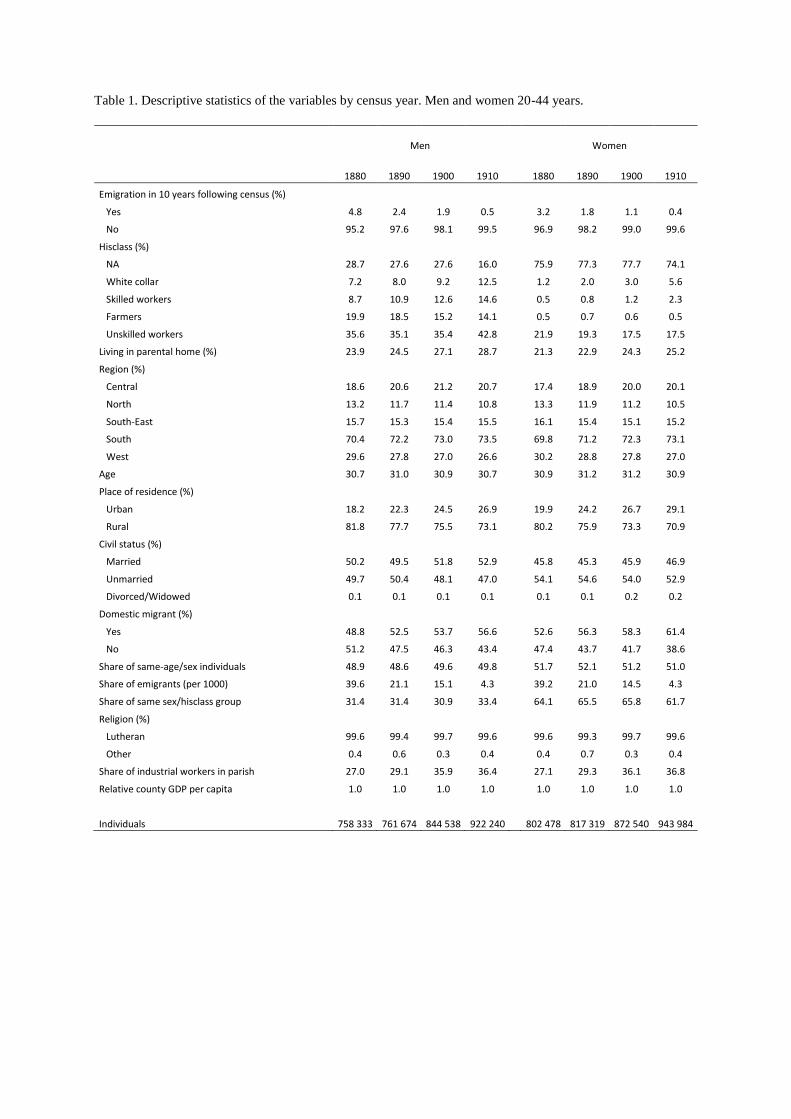
Descriptive statistics are presented in Table 1 and show a gradual decline in

emigration rates over the time period examined. In the period 1881-1890, we confidently link

4.8 and 3.2 percent of males and females, respectively, to emigration records, whereas the

figures for the 1911-1920 period are less than one percent. As expected, given that

occupational class is measured at the individual level, the majority of women have no

information (see discussion in Dribe et al. 2017). For women with a registered occupation a

great majority hold unskilled occupations, and very few are registered as farmers. This must

be kept in mind in the analysis and warrants caution in interpreting the findings for women.

For men, the distribution is expected, with an increase over time both in white-collar and

blue-collar occupations (both skilled and unskilled), at the expense of farmers. It should also

be noted that the share of individuals in the missing category decrease over time, suggesting

an increasing share of younger males in employment, despite at the same time the mean age

of the sample remaining constant, yet a larger share of the sample still living in their parental

home. A small minority of the missing class have some notation indicating a relation rather

than a proper occupation and have not been classified (e.g. son, daughter, wife). The vast

majority (97%) of the missing values result from missing occupations altogether or

occupational notations that have not been coded in HISCO due to uncertainties regarding

which occupation they refer to (abbreviations etc).

Table 1 here

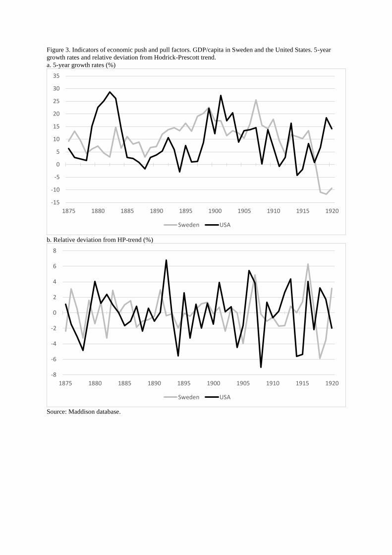
The second part of the analysis focuses on the role of push and pull factors for the

decision to migrate, using annual data on macroeconomic conditions. To exploit these annual

data, each census is expanded into a panel data set. Individuals observed in in a census and

not migrating in the subsequent ten-year period, contribute one person-year of observation for

each year of the inter-censal period. Individuals who migrate are censored upon migration and

only contributes time before migration to the risk set. Using GDP per capita (in constant

prices) for Sweden and the United States, from the Maddison database (2018), we first

measure the macroeconomic conditions as the percentage growth in GDP per capita

accumulated over the preceding five-year period. The logic behind this approach is that

individuals at the time may have been less than fully informed about the overall economic

conditions in their own country of origin, let alone some four thousand miles away. A

prolonged period of considerable economic growth (or the lack of it) should not, however,

have escaped the attention of anyone, in particular given the considerable size of the Swedish

born population in the United States already at the beginning of the study period. As an

alternative, we also use the relative deviation from a medium-term trend as a measure of the

push and pull. By processing the time series through a Hodrick-Prescott filter (factor 6.25),

the variable used expresses the relative GDP per capita variation around the trend. The

resulting series, for the time period 1875-1920, are displayed in Figure 3, showing that five-

year growth rates during the early 1880s in particular were much higher in the United States

than in Sweden. Indeed, between 1877 and 1882, the US GDP per capita grew by 29 percent,

with the Swedish growth was below 10 percent. During the 1890s, Sweden’s growth was

typically a bit higher than the one in the United States, whereas after the turn of the century

(with the exception of the last few years of the 1910s), Sweden and the United States took

turns displaying the highest five-year growth rate.

Figure 3 here

All estimates are derived from logit models of the transformed probability of

emigrating to the United States in the period of concern. In the cross-section model we study

emigration over the intercensal period (1881-1890, 1891-1900, 1901-1910 and 1911-1920),

and in the panel model we study the likelihood of emigration during one year. In all models,

standard errors are clustered at the individual level.

logit(mi)=log(mi/1-mi)=xi’β

where mi is the probability of emigrating to the United States for individual i in the time

period of concern, xi is a vector of covariates and β is the vector of parameters to be

estimated. We express the results as odds ratios derived as exp(b), where b is the estimated

regression coefficient. An odds ratio expresses the odds of emigration associated with the

category of a variable under consideration relative to the reference category (e.g. rural vs

urban), or alternatively the change in the odds of emigration associated with a one unit change

in a continuous variable (e.g., in GDP per capita).

We first look at migration selection based on individual occupational class. This will

provide a descriptive account from which occupations migrants to the United States were

primarily drawn. We first look at basic models without any control variables and then

stepwise add the full set of controls. These results will not tell us much about the causal

impact of occupational class on migration, because decisions on occupational choice and

emigration might be related and partly determined by unobserved variables, such as ability,

risk aversion, etc. As a different approach we also look at migration selection based on class

origin as measured by the occupation of the father. In this case the occupational choice (of the

father) and the decision to emigrate cannot be jointly determined. As a third approach to

migration selection, we exploit differences between siblings in occupational class and

migration propensity. Same-sex sibling combinations are by construction identified within

censuses, and census linkages across time allow us to examine individuals after they have left

their parental homes and thus embarked upon their own careers. While not exhaustively

canceling out all potential sources of bias in our estimates, exploiting between-sibling

differences allows us to obtain estimates that are free from bias from factors at the family-

level (see Abramitzky et al. 2012). Unmeasured individual-level differences between brothers

or sisters will not be captured and could still bias the estimates. In these models we restrict the

sample to siblings not residing in the parental home.

Results

Migration selection

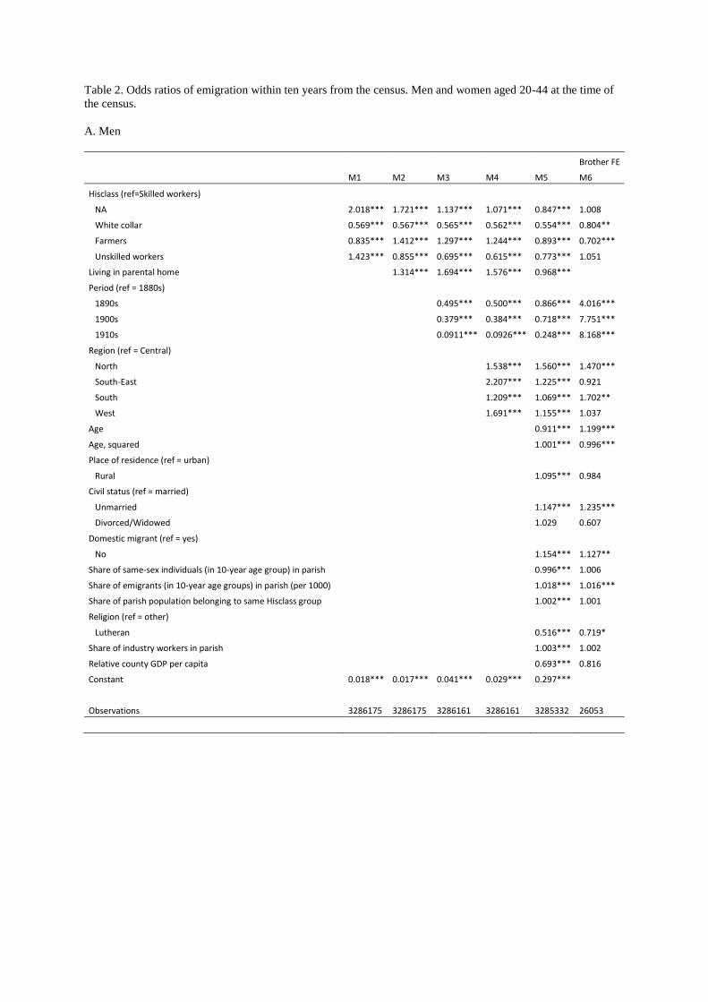
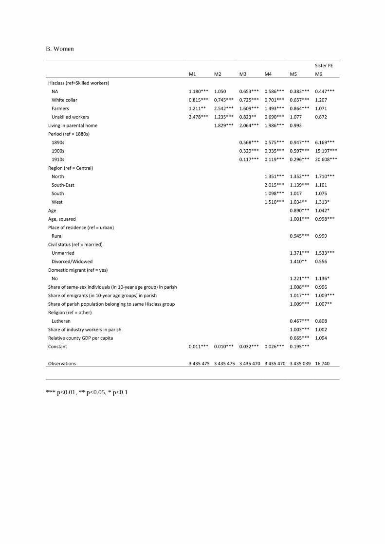
We start by looking at the cross section results where we study the probability of migrating

within the next ten years from the time of the census (1880, 1890, 1900 and 1910). Table 2

shows odds ratios for different models for men and women separately. In the basic model

without any control variables (M1), men with no occupational information and unskilled

workers have the highest migration propensity, while the white-collar groups have the lowest.

When adding a control for living in the parental home, farmers and those without an

occupation have the highest migration propensity, and white-collar groups the lowest. Blue-

collar workers are in-between, with skilled workers being somewhat more migration prone

than the unskilled. Adding the other control variables further changes the selection pattern,

but not until comprehensively controlling for both individual and contextual characteristics. In

the full model (M5), skilled workers are most prone to emigrate and the white-collar groups

least likely to do so. The other groups are in between, with the unskilled somewhat less likely

to move than the farmers. We also see that it is not controlling for time period and region that

makes the most difference, but adding the other variables (age, civil status etc). The pattern

for women is similar, with the exceptions that the group without an occupation have low

migration propensity and skilled and unskilled workers have similar migration propensities.

As was mentioned previously, however, a great majority of women are in the missing

category, which could help to explain this difference between men and women. The findings

so far seem to indicate that migrants to the United States are selected primarily among the

medium skilled, including farmers, while both the white-collar groups and the unskilled

working classes are less likely to leave Sweden for the United States.

Table 2 here

Looking at the control variables, there is a declining trend in decadal migration

propensities from the 1880s onwards, and there are also some noteworthy differences across

Swedish regions, which are both well-established in the previous literature (see Carlsson

1976). Emigration is high from the southern regions, especially from the Southwest and

Southeast, but also from the North, while it is the lowest from the central parts of Sweden

including the capital city of Stockholm. Men in rural areas are more likely to move than those

in urban areas, while the opposite is true for women for whom urban migrants dominate. The

unmarried are most likely to move, both among men and women, and among women the

previously married also have high migration propensities. People who have previously

migrated internally are less likely to emigrate, which does not seem to support ideas that

migration took place in stages from rural origins, often to domestic towns and then abroad

(see, e.g., Semmingsen 1972). More individuals of the same sex and age in the origin parish

promotes migration for women but lowers migration for men. More emigrants from the parish

in the same period increases migration propensities as does a higher share of people in the

same class. Industrialization is weakly positively related to emigration as shown by the share

of industrial workers in the place of origin. Finally, a higher than average GDP/capita in the

county of origin discourages emigration for both men and women. Overall, these findings are

line with the standard explanations of the emigration to North America.

Turning to the sibling fixed effect models (M6), the large period effects are linked to

the limited variation in this variable, since siblings tended to emigrate reasonably close

together in time. Looking at the estimates for occupational class selection for men, farmers

and white-collar workers are least likely to leave for the United States, while skilled and

unskilled workers have a similar and higher likelihood of emigration. For women, only the

lower emigration propensity of those with missing occupation is statistically significant. For

men these findings point to a selection of migrants that is stronger in the working classes, and

less pronounced among white-collar groups and farmers, while there is no consistent pattern

in terms of selection on skills within the working class. Instead, results depend on the

empirical design of each model.

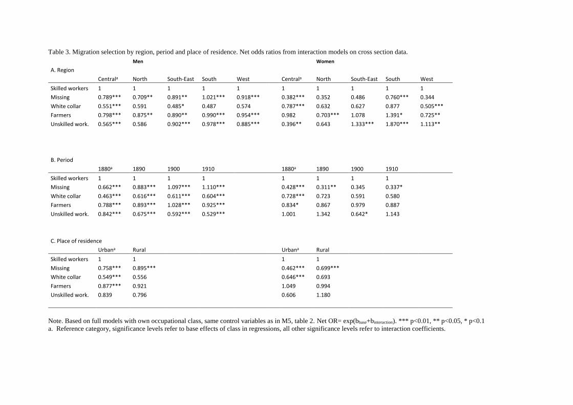
Next, we turn to the question whether the migration selection differs by region, over

time and between rural and urban areas. The estimates from interaction models on the full

sample are displayed in Table 3. Looking first at interactions between region and class, the

relatively low emigration in the white-collar group is evident in all regions to about the same

extent. The low migration propensities of the farmers and unskilled workers are most

pronounced in the Central and the North, while they are more similar to that of the skilled

workers in the southern parts. Hence, the pattern of medium-skill selection is most visible in

the Central and the North, while in the southern regions all groups except the white-collar

workers have similar propensities to migrate. For women, unskilled workers are the most

emigration prone class in the southern regions.

Table 3 here

Over time, men who are farmers become more relatively more likely to emigrate,

while unskilled workers become less likely to move, relative to skilled workers. This indicates

a less negative selection of migrants over time. Among women, there is less of a consistent

pattern over time in the selection into migration. There are no differences in the selection

pattern between rural and urban areas, except in the case of those without a registered

occupation who are relatively more likely to move when they reside in rural areas, but they

are still less likely to emigrate than the skilled workers. Hence, there is no evidence that the

selection patterns are diverging between rural and urban areas, which stands in contrast to the

findings for Norway by Abramitzky et al. (2012).

So far we have been looking at migration selection based on the individual class

position of the potential migrants. One problem with this analysis is that occupational choice

and migration might be jointly determined. As an alternative we also look at migration

selection for men and women by their social origin. Table 4 displays results from regressions

using father’s class and the same control variables as before. Father’s class was collected for

individuals linked to an earlier census when they were living in the parental home. This also

explains the large period effects, as we only have information on father’s class in 1880 for

those who still live in their parental home (who are less likely to emigrate). Comparing the

1900s and 1910s with the 1890s, the period effects are more in line with the previous results

and with expectations. More importantly, the class selection patterns are now very similar

between men and women. Sons and daughters to skilled workers are most likely to emigrate,

and those from white-collar families are least likely to move to the United States, with

farmers and unskilled in-between. Hence, the previous picture of a medium- to lower skill

selection is confirmed also when looking at origin class, but also shows notable differences

between skilled and unskilled workers.

Table 4 here

Push and pull factors

When analyzing the importance of economic cycles in the United States and Sweden, we use

the annual panel where all variables except age and the GDP variables are time-constant and

referring to the last census. Table 5 shows the results for the two different measures of push

and pull: the growth rate of GDP/capita in the previous five years, and the relative GDP/capita

deviation from trend. As before we estimated several models including different control

variables, from a simple model without controls to a fully controlled model. The estimates for

GDP/capita are similar across different model specifications, which shows that they are quite

independent of the control variables. In the full model (M6), a 1 percentage point increase in

the Swedish GDP/capita growth rate in the past five years lowers the emigration odds in the

following year by about 5 percent. A similar increase in the US growth rate instead increases

the emigration odds by almost 19 percent. If we instead look at the deviations from trend, a 1

percent higher GDP/capita in the previous year in Sweden lowers the migration odds by about

4 percent, and a similar elevated GDP in the US increases the migration odds by almost 9

percent. The figures for women are similar, which indicates that men and women are similarly

affected by the economic cycles in both Sweden and the United States. Thus, as expected,

migration is sensitive to both push and pull factors, and according to our estimates, the US

pull was more powerful than the Swedish push.

Table 5 here

The push factors also affected different occupational classes in about the same way,

for both men and women (Table 6). The only possible exception is a much weaker push for

unskilled women, when measured by the deviation from trend. All occupational classes are

also affected by the US pull, but to somewhat different degrees. For men, skilled workers and

those without a registered occupation are most affected by the US economic conditions, and

white-collar groups and unskilled workers are least affected. Among women, unskilled

workers are most affected and the while-collar groups least affected. It should be noted,

however, that all occupational classes are affected in the same direction by the US pull, and

the difference is only in the magnitude. Hence, it seems as the groups most prone to emigrate

are also the ones most affected by the US pull.

Table 6 here

Conclusion

In this paper we have taken a new look at an old question: who were the people leaving

Europe (in this case Sweden) for North America during the period of mass migration at the

turn of the last century? Previous research has focused on regional differences and differences

between countries in the timing of migration and linked it largely to economic conditions in

both sending and receiving areas. Apart from some notable research in more recent years,

there has not been many studies of the migration flows using individual-level data, trying to

determine selection patterns in more detail. To do so is important for a number of reasons.

Aggregated distributions of migrants by occupation or social class are informative to get an

idea of total flows from a country, but may not tell as much about the driving forces, as for

example regional differences in occupational structure and migration propensity may distort

the picture. Similarly, to more precisely assess the socioeconomic selection of migrants

requires careful control of other factors that have an impact on both migration and

socioeconomic attainment, such as age, marital status, contextual characteristics, etc. By using

micro-level, full count census data, linked to individual-level emigration records for Sweden

1880-1920, we studied the migration selection by occupational class and economic conditions

in both Sweden and the United States.

Given that Sweden was somewhat more unequal than the United States, as measured

by the share of income earned by the top 1 or 10 percent, we would expect migrants to have

been disproportionally selected from the lower skilled. Our findings only partly support this

prediction. The group of white-collar workers, constituting about 10 percent of our male study

population, were least likely of all groups to emigrate to the United States (except in one

specification, the brother fixed effects model, where the farmers had an even lower migration

propensity). It was a quite heterogeneous group, including the higher managers and

professionals (medical doctors, factory owners, lawyers, etc) as well as lower clerical and sale

personnel (i.e. shop assistants, lower office clerks etc). Many individuals in this group

belonged to the elite of Swedish society, with a lot to lose, and possibly not much to gain,

from moving to the United States. It is therefore expected to find that they were less likely

than other groups to move, regardless of time period, region, or detailed specification of the

empirical model. The low migration propensity in this group was clearly evident both when

we looked at selection on individual class and on father’s class.

Farmers (about 15-20 percent of out male study population depending on the census)

were mostly less likely to emigrate than the skilled workers, but more likely to emigrate than

the white-collar groups. This was particularly clear in the northern and central parts of

Sweden, and in the 1880s and 1890s. This pattern was also present for both own class and

father’s class. It is expected that farmers were less likely to pack up and leave for the United

States in the period we are studying, which largely falls after the closing of the agricultural

frontier, when most migrants headed for urban areas in the US. Therefore, it is somewhat

surprising to find similarly high migration rates for farmers and blue-collar workers, skilled as

well as unskilled, in the southern part of the country, which supplied the great majority of all

migrants. One reason for the high migration propensity of farmers in these areas could be the

increased competition from grain imports the last decades of the 1800s, which pressed

profitability of smaller farmsteads. It is also a period of a declining share of farmers in the

population, following continued industrialization and rationalization of agricultural

production.

The unskilled workers (about 35-40 percent of the male study population) were also

less likely to emigrate than the skilled workers in most specifications, except in the brother

fixed effects model where it was similar to the skilled workers. The low migration propensity

of the unskilled group was especially clear in the northern and central parts of Sweden, and in

the 1900-1920 period. It was also similar whether measured by own class or father’s class.

The unskilled workers could be expected to have most to gain from a move, as their skills

were low and hence easy to transfer to the new location, and the returns to their skills should

have been higher. However, they were supposedly also the group with the least skills to

migrate in terms of education and information. They might also have been selected among the

people with more risk aversion and lower general abilities, which may have hindered their

migration. Moreover, they might have faced the strongest financial constraints to migration.

Our findings also demonstrated the important role played by economic conditions in

both Sweden and the United States for fluctuations in migration. Both economic push and pull

factors, measured by GDP/capita, predicted migration in expected ways, which has been

shown by a number of previous studies as well. More importantly, however, out results

showed that the push and pull factors affected migration propensities in quite similar ways for

different classes. If anything, it seems that the classes with the highest migration propensities

overall, were also the ones most strongly affected by the US pull.

Finally, we attempted a comparison of the patterns for men and women. This was

made difficult for own class due to the frequent missing information on occupation for

women in the censuses. This is a well-known problem of census data in this period, not only

in Sweden, and partly reflect the low labor force participation rate of married women

especially in this period (see, e.g., Goldin 1995; Stanfors 2014; Stanfors and Goldscheider

2017). However, the censuses may also underestimate women’s participation, especially the

part time work done by many married women (see Humphries and Sarasúa 2012). About three

quarters of the women in our study population did not have a recorded occupation, which of

course distort the results of migration selection based on own occupation. Nonetheless, the

selection patterns for the groups with an occupation were usually quite similar for men and

women, and when we looked at the selection based on father’s class, the patterns for men and

women were almost identical. Hence, by and large, our analysis suggests that selection into

emigration was similar for men and women.

References

Abramitzky, R., L. P. Boustan, and K. Eriksson. 2012. Europe’s tired, poor, huddled masses:

Self-selection and economic outcomes in the age of mass migration. American Economic

Review 102: 1832-1856.

Abramitzky, R., L. P. Boustan, and K. Eriksson. 2014. A nation of immigrants: Assimilation

and economic outcomes in the age of mass migration. Journal of Political Economy 122:

467-506.

Abramitzky, R. and L. Boustan. 2017. Immigration in American economic history. Journal of

Economic Literature 55:1311-1345.

Baines, D. 1991. Emigration from Europe 1815-1930. London: Macmillan.

Barro R. J. and X. Sala-i-Martin. 1991. Convergence across States and Regions. Brookings

Papers on Economic Activity 1: 107-182.

Becker, G.S. 1964. Human Capital. Chicago: University Press.

Bohlin, J. and A-M. Eurenius. 2010. Why they moved — Emigration from the Swedish

countryside to the United States, 1881–1910. Explorations in Economic History 47: 533-

551.

Borjas, G. J. 1987. Self-selection and the earnings of immigrants. American Economic Review

77: 531-553.

Borjas, G. J. 1994. The economics of immigration. Journal of Economic Literature 32: 1667-

1717.

Boyer, G. R. 1997. Labour migration in southern and eastern England, 1861-1901. European

Review of Economic History 1:191-215.

Boyer, G. R. and T. J. Hatton. 1997. Migration and labour market integration in late

nineteenth century England and Wales. Economic History Review 50: 697-734

Carlsson, S. 1976. Chronology and composition of Swedish emigration to America. In H.

Runblom and H. Norman (eds.) From Sweden to America. A History of the Migration.

Minneapolis: University of Minnesota Press.

Chiswick, B. 1999. Are immigrants favorably self-selected? The American Economic Review,

89: 181-185.

Dribe, M. and B. Eriksson. 2018. Socioeconomic status and adult life expectancy in early

20th-century Sweden: Evidence from full-count micro census. Lund Papers in Economic

Demography 2018:1.

Dribe, M., B. Eriksson, and F. Scalone. 2017. Migration, marriage and social mobility:

women in Sweden 1880-1900. Lund Papers in Economic Demography 2017:1.

Enflo, K., M. Henning, and L. Schön. 2014. Swedish regional GDP 1855–2000: Estimations

and general trends in the Swedish regional system. In: C. Hanes and S. Wolcott (eds.),

Research in Economic History 30. Emerald Group Publishing Limited, pp. 47–89.

Eriksson, B. 2015. Dynamic Decades: A Micro Perspective on Late Nineteenth-Century

Sweden. Lund: Media-Tryck.

Eriksson, B., S. Aradhya, and F. Hedefalk. 2017. Pushing and pulling: Determinants of

migration during Sweden's industrialization. Unpublished manuscript.

Feigenbaum, J.J. 2016. A Machine Learning Approach to Census Record Linking.

Unpublished manuscript.

Goldin, C. 1995. The U-shaped female labor force function in economic development and

economic history. In T. P. Schultz (ed.) Investment in Women’s Human Capital and

Economic Development. Chicago: University of Chicago Press, pp. 60-91.

Gould, J. D. (1979). European inter-continental emigration 1815-1914: patterns and causes.

Journal of European Economic History 8: 593-679.

Harris, J. R. and M. P. Todaro. 1970. Migration, unemployment and development: A two-

sector analysis. American Economic Review 60: 126-142.

Hatton, T.J. 2010. The Cliometrics of international migration. Journal of Economic Surveys

24: 941-969.

Hatton, T. J. and J G. Williamson (1994). What Drove the Mass Migrations from Europe in

the Late Nineteenth Century? Population and Development Review 20: 533-559.

Hatton, T. J. and J. G. Williamson. 1998. The Age of Mass Migration: Causes and Economic

Impact. Oxford: Oxford University Press.

Humphries, J. and C. Sarasúa. 2012. Off the record: Reconstructing women’s labor force

participation in the European past. Feminist Economics 18:39-67

Keeling, D. The Transportation Revolution and Transatlantic Migration, 1850-1914. Research

in Economic History, 19: 39-74.

Lee, E.S. 1966. A Theory of Migration. Demography, 3: 47-57.

Long, J. 2005. Rural-urban migration and socioeconomic mobility in Victorian Britain.

Journal of Economic History 65: 1-35

Maddison Project Database, version 2018. Bolt, Jutta, Robert Inklaar, Herman de Jong and

Jan Luiten van Zanden (2018), “Rebasing ‘Maddison’: new income comparisons and the

shape of long-run economic development”, Maddison Project Working paper 10

Norström, T. 1988. Swedish emigration to the United States reconsidered. European

Sociological Review 4: 223-231.

Quigley, J. M. 1972. An economic model of Swedish emigration. Quarterly Journal of

Economics 86:111-126.

Roine, J. and D. Waldenström. 2015. Long-run trends in the distribution of income and

wealth. In A. B. Atkinson and F. Bourguignon (eds.) Handbook of Income Distribution.

Volume 2A. Amsterdam: Elsevier.

Roy, A. D. 1951. Some thoughts on the distribution of earnings. Oxford Economic Papers 3:

135-146.

Ruggles, S. 2006. Linking historical censuses: A new approach. History and Computing 14:

213-224.

Runblom, H. and H. Norman (eds.). 1976. From Sweden to America. A History of the

Migration. Minneapolis: University of Minnesota Press.

Schwartz, A. 1973. Interpreting the effect of distance on migration. Journal of Political

Economy, 81: 1153-1169.

Schön, L. 2010. Sweden’s Road to Modernity. An Economic History. Stockholm: SNS.

Semmingsen, I. 1972. Emigration from Scandinavia. Scandinavian Economic History Review

20: 45-60.

Sjaastad, L. A. 1962. The costs and returns of human migration. Journal of Political Economy

70: 80-93.

Spitzer, Y. and A. Zimran. 2018. Migrant self-selection: Anthropometric evidence from the

mass migration of Italians to the United States, 1907–1925. Journal of Development

Economics 134:226-247.

Stanfors, M. 2014. Women in a changing economy: The misleading tale of participation rates

in a historical perspective. History of the Family 19: 513-536.

Stanfors, M. and F. Goldscheider. 2017. The forest and the trees: Industrialization,

demographic change, and the ongoing gender revolution in Sweden and the United

States, 1870–2010. Demographic Research 36: 173-226.

Stoltz, Y. and J. Baten. 2012. Brain drain in the age of mass migration: Does relative

inequality explain migrant selectivity? Explorations in Economic History 49: 205-220.

Taylor, A. and J. G. Williamson. 1997. Convergence in the age of mass migration. European

Review of Economic History 1: 27-63.

Tedebrand, L.-G. 1976. Remigration from America to Sweden. In H. Runblom and H.

Norman (eds.) From Sweden to America. A History of the Migration. Minneapolis:

University of Minnesota Press.

Thomas, D.S. 1941. Social and Economic Aspects of Swedish Population Movements, 1750–

1933. New York: Macmillan.

Todaro, M. P. 1969. A model of labor migration and urban unemployment in less developed

countries. American Economic Review 59: 138-148.

Van Leeuwen, M. H. D. and I. Maas. 2011. HISCLASS. A Historical International Social

Class Scheme. Leuven: Leuven University Press.

Van Leeuwen, M. H. D., I. Maas, and A. Miles. 2002. HISCO. Historical international

standard classification of occupations. Leuven: Leuven University Press.

Wegge, S. 1998. Chain migration and information networks: evidence from nineteenth-

century Hesse-Cassel. Journal of Economic History 58:957-986.

Wegge, S. 2002. Occupational self-selection of European immigrants: Evidence from

nineteenth Hesse-Cassel. European Review of Economic History 6:365-394.

Wilkinson, M. 1967. Evidences of long swings in the growth of Swedish population and

related economic variables, 1860-1965. Journal of Economic History 27:17-38.

Figure 1. Migration totals from Sweden to the United States, 1851-1930

Figure 2. Migration events from Sweden to the United States in Emibas and linked sample, 1870-1930.

Note: Only includes first migration events.

0

5000

10000

15000

20000

25000

30000

35000

40000

45000

50000

18

51

18

54

18

57

18

60

18

63

18

66

18

69

18

72

18

75

18

78

18

81

18

84

18

87

18

90

18

93

18

96

18

99

19

02

19

05

19

08

19

11

19

14

19

17

19

20

19

23

19

26

19

29

Figure 3. Indicators of economic push and pull factors. GDP/capita in Sweden and the United States. 5-year

growth rates and relative deviation from Hodrick-Prescott trend.

a. 5-year growth rates (%)

b. Relative deviation from HP-trend (%)

Source: Maddison database.

-15

-10

-5

0

5

10

15

20

25

30

35

1875 1880 1885 1890 1895 1900 1905 1910 1915 1920

Sweden USA

-8

-6

-4

-2

0

2

4

6

8

1875 1880 1885 1890 1895 1900 1905 1910 1915 1920

Sweden USA

Table 1. Descriptive statistics of the variables by census year. Men and women 20-44 years.

Men

Women

1880 1890 1900 1910 1880 1890 1900 1910

Emigration in 10 years following census (%)

Yes 4.8 2.4 1.9 0.5 3.2 1.8 1.1 0.4

No 95.2 97.6 98.1 99.5 96.9 98.2 99.0 99.6

Hisclass (%)

NA 28.7 27.6 27.6 16.0 75.9 77.3 77.7 74.1

White collar 7.2 8.0 9.2 12.5 1.2 2.0 3.0 5.6

Skilled workers 8.7 10.9 12.6 14.6 0.5 0.8 1.2 2.3

Farmers 19.9 18.5 15.2 14.1 0.5 0.7 0.6 0.5

Unskilled workers 35.6 35.1 35.4 42.8 21.9 19.3 17.5 17.5

Living in parental home (%) 23.9 24.5 27.1 28.7 21.3 22.9 24.3 25.2

Region (%)

Central 18.6 20.6 21.2 20.7 17.4 18.9 20.0 20.1

North 13.2 11.7 11.4 10.8 13.3 11.9 11.2 10.5

South-East 15.7 15.3 15.4 15.5 16.1 15.4 15.1 15.2

South 70.4 72.2 73.0 73.5 69.8 71.2 72.3 73.1

West 29.6 27.8 27.0 26.6 30.2 28.8 27.8 27.0

Age 30.7 31.0 30.9 30.7 30.9 31.2 31.2 30.9

Place of residence (%)

Urban 18.2 22.3 24.5 26.9 19.9 24.2 26.7 29.1

Rural 81.8 77.7 75.5 73.1 80.2 75.9 73.3 70.9

Civil status (%)

Married 50.2 49.5 51.8 52.9 45.8 45.3 45.9 46.9

Unmarried 49.7 50.4 48.1 47.0 54.1 54.6 54.0 52.9

Divorced/Widowed 0.1 0.1 0.1 0.1 0.1 0.1 0.2 0.2

Domestic migrant (%)

Yes 48.8 52.5 53.7 56.6 52.6 56.3 58.3 61.4

No 51.2 47.5 46.3 43.4 47.4 43.7 41.7 38.6

Share of same-age/sex individuals 48.9 48.6 49.6 49.8 51.7 52.1 51.2 51.0

Share of emigrants (per 1000) 39.6 21.1 15.1 4.3 39.2 21.0 14.5 4.3

Share of same sex/hisclass group 31.4 31.4 30.9 33.4 64.1 65.5 65.8 61.7

Religion (%)

Lutheran 99.6 99.4 99.7 99.6 99.6 99.3 99.7 99.6

Other 0.4 0.6 0.3 0.4 0.4 0.7 0.3 0.4

Share of industrial workers in parish 27.0 29.1 35.9 36.4 27.1 29.3 36.1 36.8

Relative county GDP per capita 1.0 1.0 1.0 1.0 1.0 1.0 1.0 1.0

Individuals 758 333 761 674 844 538 922 240 802 478 817 319 872 540 943 984

Table 2. Odds ratios of emigration within ten years from the census. Men and women aged 20-44 at the time of

the census.

A. Men

Brother FE

M1 M2 M3 M4 M5 M6

Hisclass (ref=Skilled workers)

NA 2.018*** 1.721*** 1.137*** 1.071*** 0.847*** 1.008

White collar 0.569*** 0.567*** 0.565*** 0.562*** 0.554*** 0.804**

Farmers 0.835*** 1.412*** 1.297*** 1.244*** 0.893*** 0.702***

Unskilled workers 1.423*** 0.855*** 0.695*** 0.615*** 0.773*** 1.051

Living in parental home 1.314*** 1.694*** 1.576*** 0.968***

Period (ref = 1880s)

1890s 0.495*** 0.500*** 0.866*** 4.016***

1900s 0.379*** 0.384*** 0.718*** 7.751***

1910s 0.0911*** 0.0926*** 0.248*** 8.168***

Region (ref = Central)

North 1.538*** 1.560*** 1.470***

South-East 2.207*** 1.225*** 0.921

South 1.209*** 1.069*** 1.702**

West 1.691*** 1.155*** 1.037

Age 0.911*** 1.199***

Age, squared 1.001*** 0.996***

Place of residence (ref = urban)

Rural 1.095*** 0.984

Civil status (ref = married)

Unmarried 1.147*** 1.235***

Divorced/Widowed 1.029 0.607

Domestic migrant (ref = yes)

No 1.154*** 1.127**

Share of same-sex individuals (in 10-year age group) in parish 0.996*** 1.006

Share of emigrants (in 10-year age groups) in parish (per 1000) 1.018*** 1.016***

Share of parish population belonging to same Hisclass group 1.002*** 1.001

Religion (ref = other)

Lutheran 0.516*** 0.719*

Share of industry workers in parish 1.003*** 1.002

Relative county GDP per capita 0.693*** 0.816

Constant 0.018*** 0.017*** 0.041*** 0.029*** 0.297***

Observations 3286175 3286175 3286161 3286161 3285332 26053

B. Women

Sister FE

M1 M2 M3 M4 M5 M6

Hisclass (ref=Skilled workers)

NA 1.180*** 1.050 0.653*** 0.586*** 0.383*** 0.447***

White collar 0.815*** 0.745*** 0.725*** 0.701*** 0.657*** 1.207

Farmers 1.211** 2.542*** 1.609*** 1.493*** 0.864*** 1.071

Unskilled workers 2.478*** 1.235*** 0.823** 0.690*** 1.077 0.872

Living in parental home 1.829*** 2.064*** 1.986*** 0.993

Period (ref = 1880s)

1890s 0.568*** 0.575*** 0.947*** 6.169***

1900s 0.329*** 0.335*** 0.597*** 15.197***

1910s 0.117*** 0.119*** 0.296*** 20.608***

Region (ref = Central)

North 1.351*** 1.352*** 1.710***

South-East 2.015*** 1.139*** 1.101

South 1.098*** 1.017 1.075

West 1.510*** 1.034** 1.313*

Age 0.890*** 1.042*

Age, squared 1.001*** 0.998***

Place of residence (ref = urban)

Rural 0.945*** 0.999

Civil status (ref = married)

Unmarried 1.371*** 1.533***

Divorced/Widowed 1.410** 0.556

Domestic migrant (ref = yes)

No 1.221*** 1.136*

Share of same-sex individuals (in 10-year age group) in parish 1.008*** 0.996

Share of emigrants (in 10-year age groups) in parish 1.017*** 1.009***

Share of parish population belonging to same Hisclass group 1.009*** 1.007**

Religion (ref = other)

Lutheran 0.467*** 0.808

Share of industry workers in parish 1.003*** 1.002

Relative county GDP per capita 0.665*** 1.094

Constant 0.011*** 0.010*** 0.032*** 0.026*** 0.195***

Observations 3 435 475 3 435 475 3 435 470 3 435 470 3 435 039 16 740

*** p<0.01, ** p<0.05, * p<0.1

Table 3. Migration selection by region, period and place of residence. Net odds ratios from interaction models on cross section data.

Men Women

A. Region

Centrala North South-East South West Centrala North South-East South West

Skilled workers 1 1 1 1 1 1 1 1 1 1

Missing 0.789*** 0.709** 0.891** 1.021*** 0.918*** 0.382*** 0.352 0.486 0.760*** 0.344

White collar 0.551*** 0.591 0.485* 0.487 0.574 0.787*** 0.632 0.627 0.877 0.505***

Farmers 0.798*** 0.875** 0.890** 0.990*** 0.954*** 0.982 0.703*** 1.078 1.391* 0.725**

Unskilled work. 0.565*** 0.586 0.902*** 0.978*** 0.885*** 0.396** 0.643 1.333*** 1.870*** 1.113**

B. Period

1880a 1890 1900 1910 1880a 1890 1900 1910

Skilled workers 1 1 1 1 1 1 1 1 Missing 0.662*** 0.883*** 1.097*** 1.110*** 0.428*** 0.311** 0.345 0.337* White collar 0.463*** 0.616*** 0.611*** 0.604*** 0.728*** 0.723 0.591 0.580 Farmers 0.788*** 0.893*** 1.028*** 0.925*** 0.834* 0.867 0.979 0.887 Unskilled work. 0.842*** 0.675*** 0.592*** 0.529*** 1.001 1.342 0.642* 1.143

C. Place of residence

Urbana Rural Urbana Rural

Skilled workers 1 1 1 1

Missing 0.758*** 0.895*** 0.462*** 0.699***

White collar 0.549*** 0.556 0.646*** 0.693

Farmers 0.877*** 0.921 1.049 0.994

Unskilled work. 0.839 0.796 0.606 1.180

Note. Based on full models with own occupational class, same control variables as in M5, table 2. Net OR= exp(bbase+binteraction). *** p<0.01, ** p<0.05, * p<0.1

a. Reference category, significance levels refer to base effects of class in regressions, all other significance levels refer to interaction coefficients.

Table 4. Migration selection by class origin (father's occupation). Odds ratios of emigration within ten years

from the census. Men and women aged 20-44 at the time of the census.

Men Women

Origin Hisclass (ref=Skilled workers)

NA 0.774*** 0.768***

White collar 0.612*** 0.601***

Farmers 0.889*** 0.900***

Unskilled workers 0.894*** 0.895***

Living in parental home 0.955** 0.824***

Period (ref = 1880s)

1890s 4.131*** 5.693***

1900s 3.260*** 3.553***

1910s 1.390*** 2.062***

Region (ref = Central)

North 1.667*** 1.463***

South-East 1.188*** 1.133***

South 0.912*** 0.949**

West 1.136*** 1.094***

Age 0.888*** 0.855***

Age, squared 1.001*** 1.002***

Place of residence (ref = urban)

Rural 1.034** 0.903***

Civil status (ref = married)

Unmarried 1.324*** 2.124***

Divorced/Widowed 1.310 1.611*

Domestic migrant (ref = yes)

No 1.116*** 1.167***

Share of same-sex individuals (in 10-year age group) in parish 0.999 1.005***

Share of emigrants (in 10-year age groups) in parish 1.021*** 1.019***

Share of parish population belonging to same Hisclass group 1.003*** 0.999**

Religion (ref = other

Lutheran 0.552*** 0.529***

Share of industry workers in parish 1.005*** 1.004***

Relative county GDP per capita 0.623*** 0.717***

Constant 0.072*** 0.051***

Observations 2,658,488 2,723,959

*** p<0.01, ** p<0.05, * p<0.1

Table 5. Push and pull factors of Swedish emigration 1881-1919. ORs from logistic regression. Individual-level

panel data. Men and women aged 20-44 years.

M1 M2 M3 M4 M5 M6

A. Men

Sweden's GDP growth, past five years (%) 0.996 0.994 0.942 0.942 0.953 0.953

USA's GDP growth, past five years (%) 1.153 1.154 1.269 1.269 1.187 1.187

Sweden's GDP dev from trend (%) 0.978 0.978 0.964 0.964 0.960 0.960

USA's GDP dev from trend (%) 1.090 1.090 1.130 1.130 1.089 1.089

Observations 32,318,027 32,3180,27 32,318,027 32,318,027 32,318,027 32,318,027

B. Women

Sweden's GDP growth, past five years (%) 0.996 0.997 0.954 0.954 0.963 0.963

USA's GDP growth, past five years (%) 1.134 1.134 1.231 1.231 1.151 1.151

Sweden's GDP dev from trend (%) 0.992 0.992 0.986 0.986 0.978 0.978

USA's GDP dev from trend (%) 1.079 1.079 1.115 1.115 1.075 1.075

Observations 33,957,967 33,957,967 33,957,967 33,957,967 33,957,967 33,957,967

Note: All estimates are statistically significant, p<0.001.

M1: No controls

M2: Living in parental home

M3: M2+ class

M4: M3 + period and region

M5: M4 + age, civil status, migration history, proportion in same age same sex in parish, proportion of emigrants in

same age from parish, proportion same class in parish, proportion industrial workers in parish, religion

M6: M5 + relative county GDP/capita

Table 6. Push and pull factors by occupational class. Net odds ratios from interaction models.

Growth rates over past 5 years Deviation from trend

Sweden United States Sweden United States

A. Men

Skilled workersa 0.951*** 1.201*** 0.973*** 1.095***

Missing 0.953 1.207 0.959** 1.096

White collar 0.964*** 1.120*** 0.970 1.060***

Farmers 0.955*** 1.188 0.962* 1.091

Unskilled workers 0.940*** 1.133*** 0.936*** 1.063***

B. Women

Skilled workersa 0.978*** 1.149*** 0.966** 1.077***

Missing 0.960*** 1.144 0.975 1.071

White collar 0.979 1.069** 0.993 1.037**

Farmers 0.969** 1.171 0.983 1.086

Unskilled workers 0.966 1.214 1.062*** 1.103

*** p<0.01, ** p<0.05, * p<0.1 Note: Note. Based on full models with own occupational class, same control variables as in M5, table 2. Net

OR= exp(bbase+binteraction).

a. Reference category, significance levels refer to base coefficients of GDP in regressions, all other significance

levels refer to interaction coefficients.