Page 1
arX
iv:a
stro
-ph/
0609
585v
1 2
0 Se
p 20
06
DRAFT 2006.09.19: ApJ to be submitted
A Chandra Search for Coronal X Rays
from the Cool White Dwarf GD 356
Martin C. Weisskopf1, Kinwah Wu2, Virginia Trimble3,4, Stephen L. O’Dell5,
Ronald F. Elsner5, Vyacheslav E. Zavlin5,6, and Chryssa Kouveliotou5
ABSTRACT
We report observations with the Chandra X-ray Observatory of the single,
cool, magnetic white dwarf GD 356. For consistent comparison with other X-ray
observations of single white dwarfs, we also re-analyzed archival ROSAT data for
GD 356 (GJ 1205), G 99-47 (GR 290 = V1201 Ori), GD 90, G 195-19 (EG250 =
GJ 339.1), and WD 2316+123 and archival Chandra data for LHS 1038 (GJ 1004)
and GD 358 (V777 Her). Our Chandra observation detected no X rays from
GD 356, setting the most restrictive upper limit to the X-ray luminosity from
any cool white dwarf — LX < 6.0×1025 erg s−1, at 99.7% confidence, for a 1-
keV thermal-bremsstrahlung spectrum. The corresponding limit to the electron
density is n0 < 4.4×1011 cm−3. Our re-analysis of the archival data confirmed the
non-detections reported by the original investigators. We discuss the implications
of our and prior observations on models for coronal emission from white dwarfs.
For magnetic white dwarfs, we emphasize the more stringent constraints imposed
by cyclotron radiation. In addition, we describe (in an appendix) a statistical
methodology for detecting a source and for constraining the strength of a source,
which applies even when the number of source or background events is small.
Subject headings: X rays: individual (GD 356) — white dwarfs — stars: coro-
nae — radiation mechanisms: thermal — methods: statistical
1NASA Marshall Space Flight Center, VP60, Huntsville, AL 35812 ([email protected] )
2Mullard Space Science Laboratory, University College London, Holmbury St. Mary, Surrey RH5 6NT,
UK
3Dept. of Physics and Astronomy, University of California, Irvine, CA 92697-4575
4Las Cumbres Observatory, Goleta, CA 93117
5NASA Marshall Space Flight Center, VP62, Huntsville, AL 35812
6Research Fellow, NASA Postdoctoral Program (NPP)
Page 2
– 2 –
1. Introduction
Several theorists (e.g., Zheleznyakov & Litvinchuk 1984; Serber 1990; Thomas, Markiel,
& Van Horn 1995) have suggested that single, cool, magnetic white dwarfs might have coro-
nae. Some observers (Fontaine, Montmerle, & Michaud 1982; Arnaud et al. 1992; Cavallo,
Arnaud, & Trimble 1993; Musielak, Porter, & Davis 1995; Musielak et al. 2003) have pre-
viously searched for X radiation that might be emitted by hot gas above a white-dwarf
photosphere. There were no persuasive detections, despite one false alarm — GR 290, in
archival Einstein data (Arnaud et al. 1992). We here report another upper limit, more
stringent than the previous ones, for the white-dwarf star GD 356.
Three considerations motivated these X-ray searches: (a) the preponderance of mag-
netic white dwarfs among the X-ray emitting cataclysmic variables; (b) the possibility that
some features in the optical spectra of magnetic white dwarfs might be cyclotron resonances
(Zheleznyakov & Litvinchuk 1984); and (c) the feeling that coronal heating is not so well
understood that constraints from other kinds of stars wouldn’t be worthwhile. In the special
case of GD 356, the presence of Balmer lines in emission imply at least a chromosphere, mak-
ing more plausible the existence of a corona. Magnetic fields in most of the stars examined
so far (including GD 356) are 1 MG or more, thought to be fossils from the white dwarfs’
previous lives as Ap stars. More recent measurements of variable, weaker fields in some
white dwarfs — the DBV GD 358 (Winget et al. 1994) and the DA LHS 1038 (Schmidt &
Smith 1995) — suggest non-fossil magnetism. Calculations (Thomas, Markiel, & Van Horn
1995) indicate that cool white dwarfs with convective envelopes can support α–ω dynamos
capable of generating 100-kG fields.
Section 2 reviews recent theoretical considerations; Section 3, limits from previous
searches. Next, Section 4 presents the results of our Chandra observations of GD 356;
Section 5, our re-analysis of prior ROSAT and Chandra observations of GD 356 and of other
white dwarfs. Finally, Section 6 discusses the implications of the new and re-analyzed results
and emphasizes the importance of thermal cyclotron radiation in magnetic white dwarfs (cf.
Zheleznyakov, Koryagin, & Serber 2004, and references therein).
2. Magnetic coronal activity from white dwarfs with a convective layer
White dwarfs are the class of compact objects that we presumably understand best.
Nevertheless, several fundamental issues remain unresolved. For instance, are white-dwarf
magnetic fields all relic (fossil) or are there transient field components generated by dynamos?
What excites the mysterious line emission from some white dwarfs? Are X rays from white
Page 3
– 3 –
dwarfs, when detected, simply thermal emission from a deep photosphere?
All stars show a certain degree of magnetism. Quite often, coronal activity in non-
degenerate stars demonstrates the presence of a magnetic field, presumably produced via
magnetohydrodynamic (MHD) processes. In the canonical model, an α-ω dynamo in a
convective stellar envelope generates the field; acoustic waves emerging from deep beneath
the stellar atmosphere heat the corona. In contrast, the magnetic fields of degenerate stars —
such as white dwarfs — may be fossil fields. Such a fossil field, together with a small, static
atmospheric scale height, would lead one to conclude that white dwarfs should not have
coronae. However, some studies have challenged this conclusion. For example, theoretical
arguments (Wesmael et al. 1980; Koester 2002) suggest that the cooler (Teff < 18,000 K)
DA white dwarfs and (Teff < 30,000 K) DB white dwarfs could possess a convective zone —
a necessary ingredient for coronal X-ray emission. Further, differential rotation, if it occurs
in white dwarfs (cf. Kawaler, Sekii, & Gough 1999), might support a magnetic dynamo. As
noted above, the magnetic-field strength generated by an α–ω dynamo in a cool white dwarf
might approach 100 kG (Thomas, Markiel, & Van Horn 1995).
Most important is the presence of emission lines from some white dwarfs with no de-
tectable companion. Among these, and thus especially interesting, are the H-Balmer line
emission from the nearby (21.1 pc) white dwarf GD 356 (Greenstein & McCarthy 1985) and
the metal lines from G227-5 and from G35-26 (Provencal, Shipman, & MacDonald 2005).
For single white dwarfs, such emission lines indicate some chromospheric activity. Alterna-
tive models for the H emission lines in GD 356 include accretion of the interstellar medium
and the presence of an interacting companion star or even a planet (Greenstein & McCarthy
1985; Li, Wickramasinghe, & Ferrario 1998). The estimated luminosity of the Zeeman-split
Hα emission lines of GD 356 is ≈ 2.1 × 1027 erg s−1. Further, the flat Balmer decrement
(f(Hα)/f(Hβ) ≈ 1.2, Greenstein & McCarthy 1985) excludes photo-ionization and recom-
bination in an optically thin gas, suggesting instead a dense emission region with electron
number density ne ≈ 1014 cm−3 (Greenstein & McCarthy 1985). A possible cause of the
chromospheric Balmer line emission is irradiation by UV/X rays from a hot magnetic corona
above the cooler white-dwarf atmosphere. The presence of a white-dwarf magnetic corona
remains unverified, which motivated our Chandra observation. However, reported temporal
variations of the magnetic field of (DBV) GD 358 (Winget et al. 1994) and of (DA) LHS 1038
(Schmidt & Smith 1995) are consistent with a magnetic corona.
In addition to facilitating the MHD dynamo process, a convective zone (Bohm &
Cassinelli 1971) also results in acoustic-wave generation. Calculations show that the flux
of such acoustic waves can be as large as ≈1010 erg cm−2 s−1 (Musielak 1987). If the acous-
tic energy reaches the white-dwarf surface unabsorbed, it can provide a total luminosity
Page 4
– 4 –
≈ 5×1028 erg s−1. However, due to radiative damping and wave trapping, a substantial
fraction of this acoustic energy will not reach the white-dwarf atmosphere. For cool DA
and DB white dwarfs with sensible parameters, fast-mode acoustic waves would attenuate
to a negligible level at the white-dwarf atmosphere (Musielak 1987), thus failing to power
a magnetic corona. Instead, wave trapping excites p-mode stellar pulsations (Musielak &
Fontenla 1989). In contrast, if the white dwarf is magnetic (but not so much as to suppress
convection), transverse slow modes can propagate, carrying perhaps 60%–80% (Musielak
1987) of the wave energy into the stellar atmosphere.
3. Previous X-ray observations
The detection of X radiation from Sirius B (Mewe et al. 1975) established that white
dwarfs are soft-X-ray sources. Subsequent Einstein, EXOSAT and ROSAT observations (e.g.,
Musielak 1987; Kahn et al. 1984; Petre, Shipman, & Canizares 1986; Paerels & Heise 1989;
Koester et al. 1990; Kidder et al. 1992; Barstow, et al. 1993) detected X radiation from a num-
ber of hot (Teff > 30,000 K) white dwarfs. Thermal emission from the photosphere (Shipman
1976) accounts for the X-ray emission in all but one case: For the (DO) KPD 0005+5106,
optically thin thermal emission better fits the observed ROSAT data (Fleming, Werner,
& Barstow 1993), indicating a hot tenuous plasma layer enveloping the white dwarf. For
KPD 0005+5106, the inferred temperature of the X-ray emitting plasma is 0.2–0.3 MK,
lower than the typical temperature of magnetic coronae around late-type stars and perhaps
indicating a hot wind resembling those of O/B stars.
Searches, with Einstein and EXOSAT (Fontaine, Montmerle, & Michaud 1982; Arnaud
et al. 1992) and with ROSAT (Cavallo, Arnaud, & Trimble 1993; Musielak, Porter, & Davis
1995), for coronal X rays from cool white dwarfs yielded no firm detections. For searches with
the ROSAT Position-Sensitive Proportional Counter (PSPC), Cavallo, Arnaud, & Trimble
(1993) established X-ray upper limits for the white dwarfs G 99-47 and G 195-19; Musielak,
Porter, & Davis (1995), for GD 90, GD 356, and WD 2316+123. Likewise, observations
(Musielak et al. 2003) with the Chandra Advanced CCD Imaging Spectrometer (ACIS) of
reportedly magnetically-varying white dwarfs, detected X radiation neither from LHS 1038
nor from GD 358. Table 1 summarizes some relevant general properties of these white dwarfs:
Column 1 gives the name; columns 2 and 3, the epoch-2000 right ascension RA(J2000) and
declination Dec(J2000); columns 4 and 5, the proper-motion components; column 6, the
distance; column 7, the spectral type; and columns 8 and 9, the surface effective temperature
and magnetic field.
The previous searches determined upper limits to the X-ray luminosity for a thermal-
Page 5
– 5 –
bremsstrahlung spectrum with negligible interstellar absorption. Assuming a coronal tem-
perature of 11.6 MK (1.0 keV), Cavallo, Arnaud, & Trimble (1993) obtained ROSAT-PSPC
99%-confidence limits to the 0.1–2.5-keV luminosity of < 2.9×1026 erg s−1 for G 99-47 and
< 1.4×1026 erg s−1 for G 195-19. Assuming a coronal temperature of 2.5 MK (0.215 keV),
Musielak, Porter, & Davis (1995) obtained ROSAT-PSPC 99.7-%-confidence (3-σ) limits
to the 0.1–2.4-keV luminosity of < 7.8×1027 erg s−1 for GD 90, < 4.4×1026 erg s−1 for
GD 356, and < 3.4×1027 erg s−1 for WD 2316+123. Under the same assumptions but using
Chandra-ACIS observations, Musielak et al. (2003) found < 4.3×1026 erg s−1 for LHS 1038
and < 4.3×1027 erg s−1 for GD 358. These upper limits were comparable to the X-ray lumi-
nosities that Musielak et al. (2003) had predicted for LHS 1038 and GD 358 — 5×1026 erg s−1
and 5×1027 erg s−1, respectively. For uniform comparison of results over a wider range of
assumed parameters, we re-analyzed (§5 and Table 2) the relevant archived Chandra (§5.1)
and ROSAT (§5.2) data.
4. The Chandra observation of GD 356
We obtained a 31.8-ks Chandra observation (ObsID 4484, 2005 May 24) using the Ad-
vanced CCD Imaging Spectrometer (ACIS) S3 (back-illuminated) CCD in the faint, timed-
exposure mode, with 3.141-s frame time. Background levels were nominal throughout the
observation. Standard Chandra X-ray Center (CXC) processing (ASCDS version number
CIAO3.2) provided level-2 event files. In analyzing data, we utilized events in pulse-invariant
channels corresponding to 0.5 to 8.0 keV.
Our Chandra observation found no X rays in a 1′′-radius detect cell at the epoch-
2005.39 position of GD 356 — 16h 40m 57.s23 +53 41′ 8.′′6, after adjustment of the epoch-
2000 coordinates for proper motion (Table 1). The nearest detected X-ray source — #6
in Table 3 — lies 46′′ from GD 356. To determine the background, we “punched out” the
detected X-ray sources eliminating all counts within a 20-σ radius of each position in Table 3.
Table 2 summarizes the results for our Chandra observation of GD 356, as well as for our re-
analysis (§5) of previous Chandra (§5.1) and ROSAT (§5.2) searches for X-ray emission from
this and other single white dwarfs. Column 1 lists the name of the white dwarf; column 2,
the observatory used; column 3, the epoch relative to 2000.00 (used to adjust for proper
motion); and column 4, the integration time. Column 5 presents the number of detected
counts mT in the “Target” (detect) cell T and column 6, its solid angle ΩT . Analogously,
column 7 presents the number of detected counts mR in the “Reference” region R and
column 8, its solid angle ΩR. Finally, columns 9, 10, 11, and 12 list the confidence level for
detection of a source (§A.2), the 99.7%-confidence upper limit on the expectation value of the
Page 6
– 6 –
number of source counts (§A.3), and the corresponding limits on the X-ray luminosity (for
a 1-keV thermal-bremsstrahlung spectrum) and on the electron density, which follow from
the analysis below. Owing to the very small (1-′′ radius) detect cell afforded by Chandra’s
sub-arcsecond resolution, only two (2) counts in the Target aperture would have constituted
a (3-σ) 99.7%-confidence detection for either of the three Chandra data sets! Neither of the
three Chandra observations found an event in the detect cell.
A statistical analysis (Appendix A) of the data yields (Equation A8) the confidence
level for detection of a source within the Target (detect) cell and (Equation A22) a 99.7%-
confidence upper limit to the expected number of source counts in the Target (detection) cell
T . Before converting the source counts to a flux and luminosity, we correct for the fraction
of the point spread function (PSF) outside the detect cell. For Chandra and almost any
soft spectrum, about 90%1 of the source photons for an on-axis source would lie within the
chosen detect cell. To convert the resulting 5-count (4.5/0.9) limit to a flux, we calculated
the redistribution matrix (rmf) and effective area (arf) functions appropriate to the loca-
tion of GD 356 in the focal plane, using the Chandra CIAO 3.3 software tools mkacisarmf
and mkarf, following the analysis thread2 for creating these functions for a specific location.
Assuming a column NH = 5×1018 cm−2 and a thermal bremsstrahlung spectrum, we used
XSPEC (v11.3.2)3 with abund set to wilm, xsect set to vern, and tbabs(bremss) as the
model. For each assumed value for the coronal temperature, we adjusted the model normal-
ization until the absorbed flux produced 5.0 counts in the S3 detector in the observing time
of the Chandra observation. Feeding this normalization into XSPEC, we used the dummyrsp
feature to calculate the flux for 104 bins over the energy range 10−5 keV to 100 keV. We
used this approach to improve the accuracy of our flux calculations since the instrument
response is calculated over a more restricted energy range, and with cruder energy bins. We
then calculated fluxes over the band from 0.01 to 100 keV, now setting the column density
to zero to obtain the unabsorbed flux.
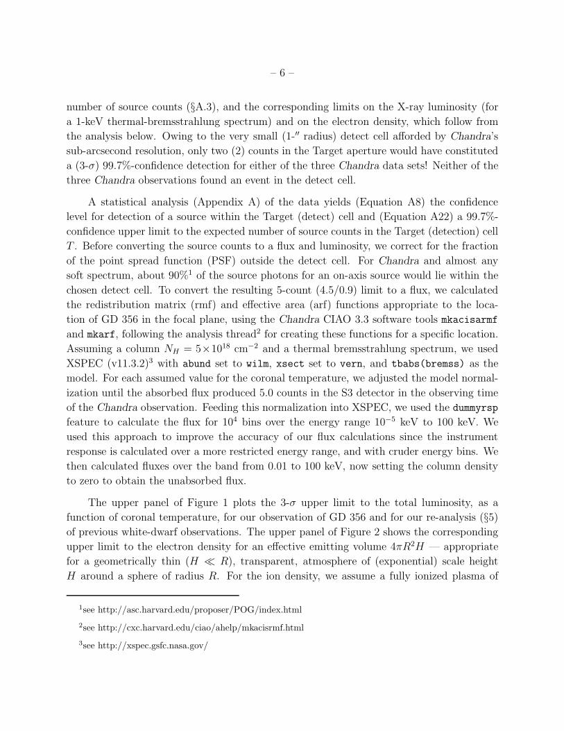
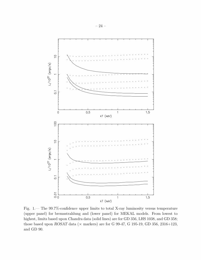
The upper panel of Figure 1 plots the 3-σ upper limit to the total luminosity, as a
function of coronal temperature, for our observation of GD 356 and for our re-analysis (§5)
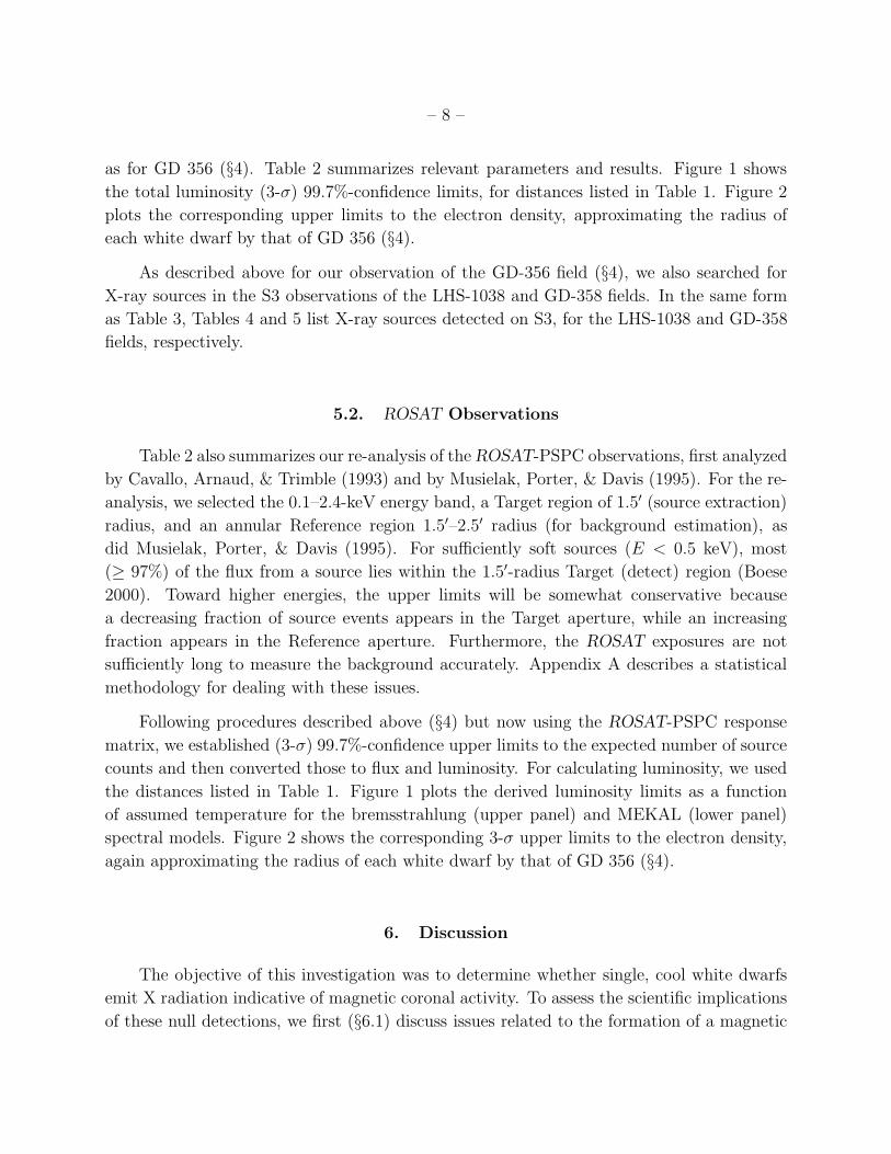
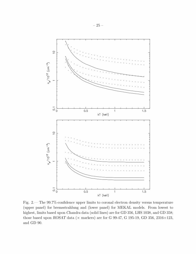
of previous white-dwarf observations. The upper panel of Figure 2 shows the corresponding
upper limit to the electron density for an effective emitting volume 4πR2H — appropriate
for a geometrically thin (H ≪ R), transparent, atmosphere of (exponential) scale height
H around a sphere of radius R. For the ion density, we assume a fully ionized plasma of
1see http://asc.harvard.edu/proposer/POG/index.html
2see http://cxc.harvard.edu/ciao/ahelp/mkacisrmf.html
3see http://xspec.gsfc.nasa.gov/
Page 7
– 7 –
hydrogen and helium with nHe/nH = 0.1, such that∑
niZ2i = 1.4ne. The bremsstrahlung
emissivity then goes as 1.4n2e = 1.4n2
0/2, where n0 is the electron density at the base of
an isothermal corona. Note that only about half the coronal emission emerges, due to
photospheric absorption of most of the downward coronal flux. Using GD 356’s 21.1-pc
parallax distance (van Altena, Lee, & Hoffleit 1995) and published UBV (Mermilliod &
Mermilliod 1994) and JHK (Skrutskie et al. 2006) photometry, we obtain the photospheric
temperature Ts = 7840 K and radius R = 0.0105R⊙ = 7.34×108 cm. For the coronal scale
height, we use H = (2×107 cm) kT/(1 keV), corresponding to a surface gravity log[g(cgs)]
= 8. The lower panels of Figures 1 and 2 display analogous limits for the tbabs(mekal)
Mewe–Kaastra–Liedahl (MEKAL) model with parameters as above, but abund set to lodd.
Besides examining the white-dwarf location for X rays, we searched for X-ray sources
anywhere on S3 employing techniques described in Tennant (2006). For the 31.8-ks Chan-
dra observation, Table 3 lists the X-ray properties of the 23 detected sources, each desig-
nated with a source number in column 1. Columns 2–5 give, respectively, right ascension
RA(J2000), declination Dec(J2000), extraction radius θext, and approximate number of X-ray
counts mD detected from the source. The single-axis RMS error in the X-ray-source position
is σX = [(σ2PSF/mD)+σ2
sys]1/2, where mD is the approximate number of detected events above
background, σPSF is the dispersion of the circular Gaussian that approximately matches the
PSF at the source location, and σsys is a systematic error. Uncertainties in the plate scale4
imply σsys ≈ 0.′′13: To be conservative, we set σsys = 0.′′2 (per axis). Column 6 gives the
radial uncertainty θ99 = 3.03 σX in the X-ray position — i.e., χ22 = 9.21 = 3.032 corresponds
to 99% confidence on 2 degrees of freedom, for inclusion of the true source position.
5. Re-analysis of previous observations.
For consistent comparison of X-ray observations, we also re-analyzed certain prior Chan-
dra (§5.1) and ROSAT (§5.2) observations of single, cool white dwarfs. The Chandra obser-
vations used the ACIS-S instrument; the ROSAT observations, the PSPC.
5.1. Prior Chandra Observations
We re-processed and analyzed previous Chandra observations of the cool white dwarfs
LHS 1038 (ObsID 1864, 5.88 ks) and GD 358 (ObsID 1865, 4.88 ks), in the same manner
4See http://asc.harvard.edu/cal/hrma/optaxis/platescale/
Page 8
– 8 –
as for GD 356 (§4). Table 2 summarizes relevant parameters and results. Figure 1 shows
the total luminosity (3-σ) 99.7%-confidence limits, for distances listed in Table 1. Figure 2
plots the corresponding upper limits to the electron density, approximating the radius of
each white dwarf by that of GD 356 (§4).
As described above for our observation of the GD-356 field (§4), we also searched for
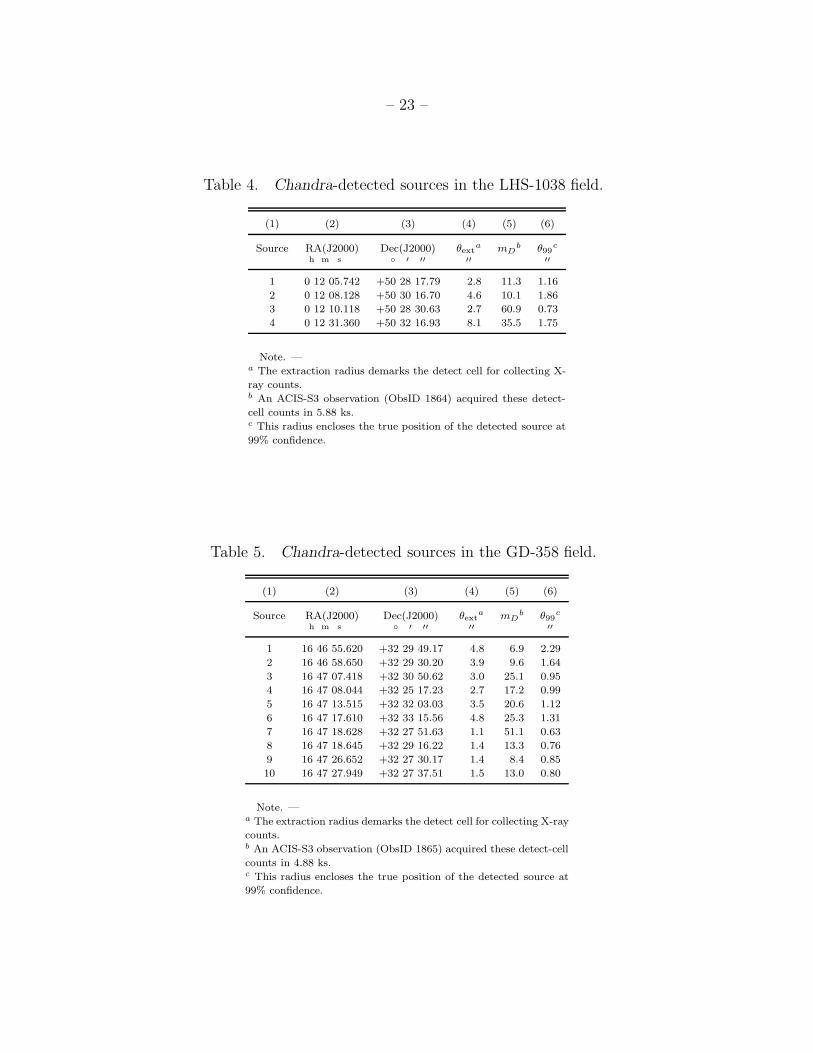
X-ray sources in the S3 observations of the LHS-1038 and GD-358 fields. In the same form
as Table 3, Tables 4 and 5 list X-ray sources detected on S3, for the LHS-1038 and GD-358
fields, respectively.
5.2. ROSAT Observations
Table 2 also summarizes our re-analysis of the ROSAT-PSPC observations, first analyzed
by Cavallo, Arnaud, & Trimble (1993) and by Musielak, Porter, & Davis (1995). For the re-
analysis, we selected the 0.1–2.4-keV energy band, a Target region of 1.5′ (source extraction)
radius, and an annular Reference region 1.5′–2.5′ radius (for background estimation), as
did Musielak, Porter, & Davis (1995). For sufficiently soft sources (E < 0.5 keV), most
(≥ 97%) of the flux from a source lies within the 1.5′-radius Target (detect) region (Boese
2000). Toward higher energies, the upper limits will be somewhat conservative because
a decreasing fraction of source events appears in the Target aperture, while an increasing
fraction appears in the Reference aperture. Furthermore, the ROSAT exposures are not
sufficiently long to measure the background accurately. Appendix A describes a statistical
methodology for dealing with these issues.
Following procedures described above (§4) but now using the ROSAT-PSPC response
matrix, we established (3-σ) 99.7%-confidence upper limits to the expected number of source
counts and then converted those to flux and luminosity. For calculating luminosity, we used
the distances listed in Table 1. Figure 1 plots the derived luminosity limits as a function
of assumed temperature for the bremsstrahlung (upper panel) and MEKAL (lower panel)
spectral models. Figure 2 shows the corresponding 3-σ upper limits to the electron density,
again approximating the radius of each white dwarf by that of GD 356 (§4).
6. Discussion
The objective of this investigation was to determine whether single, cool white dwarfs
emit X radiation indicative of magnetic coronal activity. To assess the scientific implications
of these null detections, we first (§6.1) discuss issues related to the formation of a magnetic
Page 9
– 9 –
corona around a white dwarf. We then (§6.2) examine the rather severe constraints that
cyclotron emission lines and radiative loss impose on a corona around a cool magnetic white
dwarf, such as GD 356. Finally (§6.3), we summarize our results and conclusions about
hypothesized hot coronae around magnetic white dwarfs.
6.1. Formation of a Corona
The existence of coronae around single, cool white dwarfs remains an unsettled issue:
This, of course, motivated our search for X-ray evidence. Here we briefly address some
questions relevant to the formation of a magnetic corona.
1. Is there a convection zone? Theoretical studies have indicated that convection can
occur in white dwarfs for certain temperature ranges. Analyses of white-dwarf at-
mospheric elemental abundance also evidence convective activity. Thus, it is quite
plausible that some white dwarfs possess a convection zone that generates acoustic
waves.
2. How much acoustic wave energy is generated in the convection zone? Calculations
(Musielak 1987; Winget et al. 1994) have shown that the convection-generated acoustic
flux could exceed 108 erg cm−2 s−1 and may reach 1010 erg cm−2 s−1 for DA white dwarfs
and 1011 erg cm−2 s−1 for DB white dwarfs.
3. What fraction of the acoustic wave energy is transmitted to the white-dwarf surface?
For white dwarf with a substantial magnetic field (B ≈ 104 G or higher), more than
half of the wave energy generated in the convection zone can reach the white-dwarf
atmosphere. If all the wave energy is converted into coronal X rays, the expected
luminosity will be ≈ 1027−1030 erg s−1. Our upper limit to the X-ray luminosity for
GD 356 is an order of magnitude below 1027 erg s−1 over most of the range of assumed
temperatures. This implies either that the putative convection zone generates less
acoustic energy, that the efficiency of acoustic-wave transmission to the surface is
smaller, or that a corona fails to form even if the acoustic energy reaches the white-
dwarf surface.
4. Can a magnetic corona form, given sufficient energy provided by the acoustic flux? The
null detection of coronal X rays from white dwarfs has led some (see e.g., Musielak,
Winget, & Montgomery 2005) to suggest that the emerging acoustic flux causes chro-
mospheric activity rather than formation of a hot corona. An example of such chromo-
spheric activity would be oscillations resulting from the stellar atmosphere to propa-
gating acoustic waves in the presence of a temperature inversion (Musielak, Winget, &
Page 10
– 10 –
Montgomery 2005). Whether acoustic waves generate chromospheric activity remains
unverified. Nevertheless, a number of systems exhibit chromospheric activity. The
luminosity of Hα emission lines in GD 356 is ≈ 1.8×1027 erg s−1 (see Greenstein &
McCarthy 1985). Our Chandra observation eliminates the possibility that irradiation
of the atmosphere by coronal X rays powers the Balmer lines. Further, it is not clear
that atmospheric oscillations can account for the luminosity of Balmer emission lines
in GD 356.
While coronal X radiation from cool (Teff < 10, 000 K) magnetic white dwarfs remains
undetected, X radiation from hot optically thin thermal plasmas appears to occur from
very hot (1.2 × 10⁵ K) white dwarf KPD 0005+5106. Now the question is this: Without a
magnetic corona, what supports the hot plasma envelope in the strong gravitational field of
the white dwarf? Radiation driven envelopes — predicted for hot white dwarfs (Bespalov &
Zheleznyakov 1990; Zheleznyakov, Serber, & Kuijpers 1996) — could provide this support.
Provided the white dwarf has a strong magnetic field, cyclotron-resonance radiation pressure
from photospheric radiation could drive the wind, with an estimated mass-loss rate ≈ 2×
1010 g s−1. Thus, a hot magnetic white dwarf could emit X rays from an optically thin,
thermal plasma in a radiation-driven outflow.
6.2. Cyclotron Radiation
The Chandra observation sets stringent constraints on a supposed hot corona above the
white-dwarf atmosphere. For GD 356, the X-ray luminosity LX < 6.0×1025 erg s−1 and
electron number density n0 < 4.4×1011 cm−3 at the base of a corona of (exponential) scale
height of 2.0×107 cm for a 1-keV plasma. However, for a magnetic white dwarf, Zheleznyakov,
Koryagin, & Serber (2004) note that electron-cyclotron emission lines and radiative losses
even more severely constrain the parameters of a hypothesized hot corona.
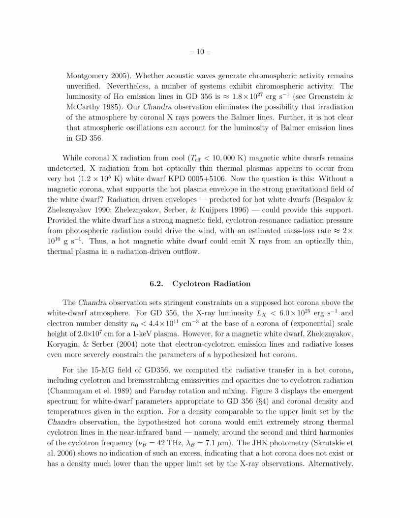
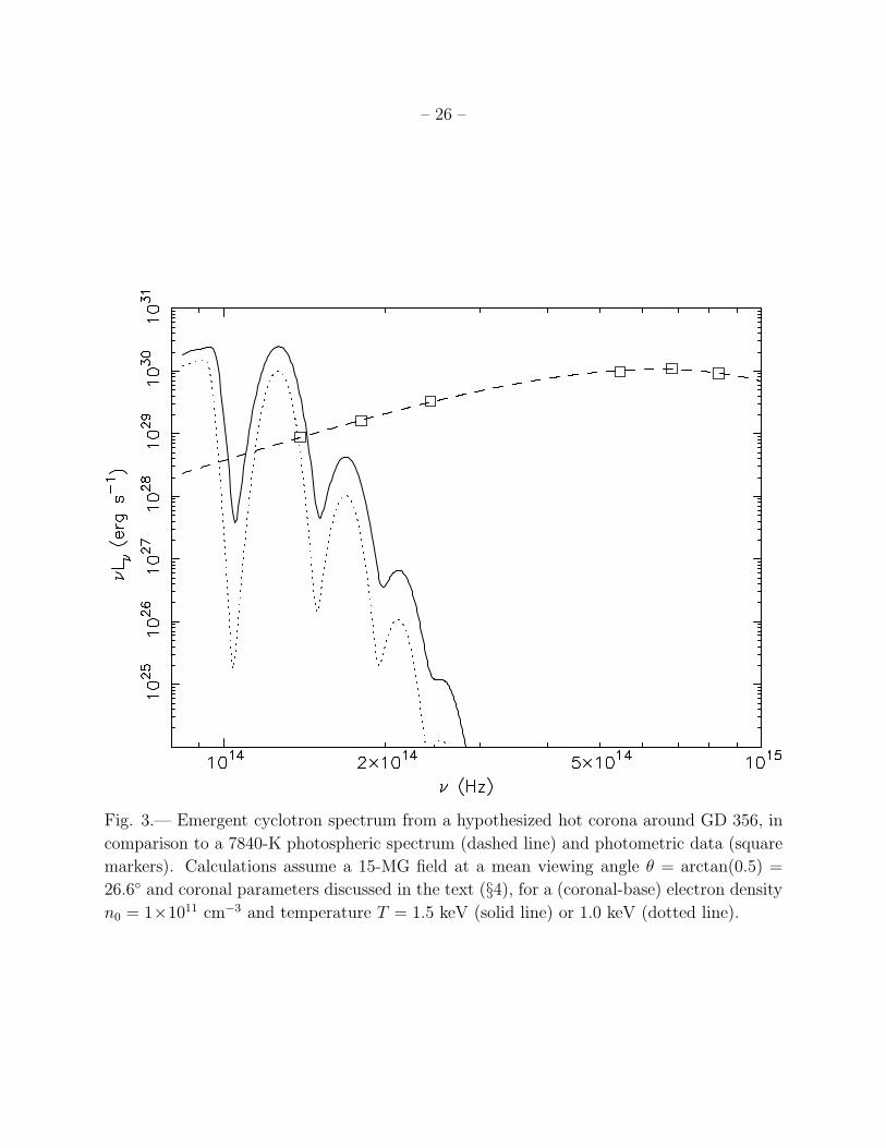
For the 15-MG field of GD356, we computed the radiative transfer in a hot corona,
including cyclotron and bremsstrahlung emissivities and opacities due to cyclotron radiation
(Chanmugam et el. 1989) and Faraday rotation and mixing. Figure 3 displays the emergent
spectrum for white-dwarf parameters appropriate to GD 356 (§4) and coronal density and
temperatures given in the caption. For a density comparable to the upper limit set by the
Chandra observation, the hypothesized hot corona would emit extremely strong thermal
cyclotron lines in the near-infrared band — namely, around the second and third harmonics
of the cyclotron frequency (νB = 42 THz, λB = 7.1 µm). The JHK photometry (Skrutskie et
al. 2006) shows no indication of such an excess, indicating that a hot corona does not exist or
has a density much lower than the upper limit set by the X-ray observations. Alternatively,
Page 11
– 11 –
the magnetic field could be somewhat weaker than 15 MG, which would shift the strong
third harmonic (ν3 = 126 THz, λ3 = 2.4 µm) to a lower frequency, longward of the Ks band.
Nevertheless, our calculation confirms the conclusion of Zheleznyakov, Koryagin, & Serber
(2004): Infrared–visible spectrophotometry is potentially a powerful probe of any hot corona
around a magnetic white dwarf.
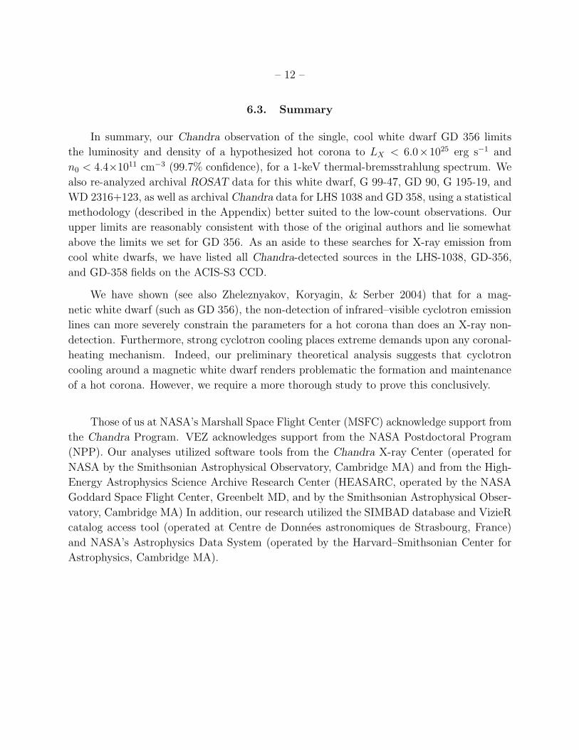
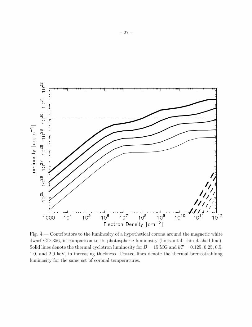
In addition to producing potentially detectable emission lines, thermal cyclotron radi-
ation would be the dominant cooling mechanism in a hot corona around a magnetic white
dwarf. Figure 4 displays the radiated thermal cyclotron and bremsstrahlung luminosity for
a supposed isothermal corona around GD 356 (B = 15 MG), as a function of density for
various electron temperatures between 0.125 keV and 2.0 keV. As the plot clearly shows,
cyclotron cooling dramatically exceeds bremsstrahlung cooling for a hot, tenuous plasma
above a magnetic white dwarf. Indeed, for GD 356, the coronal thermal cyclotron luminos-
ity rivals the photospheric luminosity unless the electron density is very much less than the
upper limit set by the X-ray observation.
Strong cyclotron cooling above a magnetic white dwarf imposes severe demands upon
any coronal heating mechanism. As Figure 4 demonstrates, even the weak requirement
(Zheleznyakov, Koryagin, & Serber 2004) that the coronal thermal cyclotron luminosity
not exceed the photospheric luminosity limits the electron density to n0 < 3×109 cm−3 for
kT = 1 keV. If an acoustic flux as large as 1010 erg cm−2 s−1 (Musielak 1987) efficiently heats
a corona around GD 356, this heating rate can balance cyclotron cooling for n0 ≈ 3×105 cm−3
for kT = 1 keV. This is about 6-orders-of-magnitude less than the density limit set by X-ray
non-detection!
For an electron density n0 < 3×106 cm−3 — approximately independent of temper-
ature — a corona above the white-dwarf photosphere would be transparent to cyclotron
radiation in the 15-MG field of GD 356. However, when transparent, the cyclotron cooling
time — again approximately independent of temperature — is only 2 µs in this magnetic
field. For electron densities and temperatures of interest, the mean time between colli-
sions — about (1.4×10⁹ s cm−3) (kT/(1 keV))1.5 ne−1 — is much longer than this cyclotron
cooling time. Thus, the plasma would not be in local thermodynamic equilibrium (LTE,
Zheleznyakov, Koryagin, & Serber 2004, and references therein), unless some collisionless
process — e.g., scattering by Alfven waves — intervenes to transfer energy to the electrons’
transverse degrees of freedom, on this very short timescale.
Page 12
– 12 –
6.3. Summary
In summary, our Chandra observation of the single, cool white dwarf GD 356 limits
the luminosity and density of a hypothesized hot corona to LX < 6.0×1025 erg s−1 and
n0 < 4.4×1011 cm−3 (99.7% confidence), for a 1-keV thermal-bremsstrahlung spectrum. We
also re-analyzed archival ROSAT data for this white dwarf, G 99-47, GD 90, G 195-19, and
WD 2316+123, as well as archival Chandra data for LHS 1038 and GD 358, using a statistical
methodology (described in the Appendix) better suited to the low-count observations. Our
upper limits are reasonably consistent with those of the original authors and lie somewhat
above the limits we set for GD 356. As an aside to these searches for X-ray emission from
cool white dwarfs, we have listed all Chandra-detected sources in the LHS-1038, GD-356,
and GD-358 fields on the ACIS-S3 CCD.
We have shown (see also Zheleznyakov, Koryagin, & Serber 2004) that for a mag-
netic white dwarf (such as GD 356), the non-detection of infrared–visible cyclotron emission
lines can more severely constrain the parameters for a hot corona than does an X-ray non-
detection. Furthermore, strong cyclotron cooling places extreme demands upon any coronal-
heating mechanism. Indeed, our preliminary theoretical analysis suggests that cyclotron
cooling around a magnetic white dwarf renders problematic the formation and maintenance
of a hot corona. However, we require a more thorough study to prove this conclusively.
Those of us at NASA’s Marshall Space Flight Center (MSFC) acknowledge support from
the Chandra Program. VEZ acknowledges support from the NASA Postdoctoral Program
(NPP). Our analyses utilized software tools from the Chandra X-ray Center (operated for
NASA by the Smithsonian Astrophysical Observatory, Cambridge MA) and from the High-
Energy Astrophysics Science Archive Research Center (HEASARC, operated by the NASA
Goddard Space Flight Center, Greenbelt MD, and by the Smithsonian Astrophysical Obser-
vatory, Cambridge MA) In addition, our research utilized the SIMBAD database and VizieR
catalog access tool (operated at Centre de Donnees astronomiques de Strasbourg, France)
and NASA’s Astrophysics Data System (operated by the Harvard–Smithsonian Center for
Astrophysics, Cambridge MA).
Page 13
– 13 –
A. Statistical Methodology
Statistical estimates of source and background counts and their errors often merely
approximately describe an observation or apply only in the large-number limit. Here we
present a statistical methodology that more generally describes apertured data (including
allowing for uncertainty in the background) and makes no large-number assumption. First
(§A.1) we obtain the probability distribution that accurately describes the observation and
provides the basis for the statistical analyses to follow. We then describe an appropriate
statistical test for detection of a source (§A.2) and one for constraining the expectation
value for the number of source events (§A.3).
A.1. Probability for Observed Events
We characterize a measurement (realization) in terms of the observed number of events
(counts) mT and mR in disjoint regions (apertures) T and R of known measure (solid-angle,
area, wavelength band, time interval, etc., as appropriate) ΩT and ΩR, respectively. We
regard T as a “Target” aperture that may contain a source with an expectation value mS
events (counts); R as a “Reference” aperture that contains no source. Although no source
lies within R, source events may occur in R if their distribution is not delta-distributed —
i.e., confined to a point. Thus, we define ΨT and ΨR to be the known fractions of source
events in the Target T and Reference R apertures, such that the expectation values for the
number of source events are mSΨT and mSΨR, respectively. In addition to source events,
apertures T and R contain background (non-source) events, with expectation values µBΩT
and µBΩR, with µB the expectation value for the density (per unit measure) of background
events. For convenience, we denote with a subscripted “U” parameters or values over the
combined aperture U ≡ T ∪R, with T ∩ R = 0 — namely, ΩU = ΩT + ΩR, ΨU = ΨT + ΨR,
and mU = mT +mR.
Consequently, the expectation values for the number of events (counts) in apertures T
and R are mT and mR, respectively:
mT = mSΨT + µBΩT , (A1)
mR = mSΨR + µBΩR . (A2)
Hence, the probability for mT and mR events in an observation (realization) is
PmT ,mR(mT , mR) = [ mmT
T e−mT /mT ! ] × [ mmR
R e−mR/mR! ] . (A3)
Upon substituting Equations A1 and A2 into Equation A3,
PmT ,mR(mS, µB; ΨT ,ΨR,ΩT ,ΩR) = [ (mSΨT + µBΩT )mT e−(mSΨT +µBΩT )/mT ! ] ×
Page 14
– 14 –
[ (mSΨR + µBΩR)mR e−(mSΨR+µBΩR)/mR! ] . (A4)
Given values for the known parameters (ΨT , ΨR, ΩT , and ΩR) and for the observed number
of events (mT and mR) in each aperture, Equation A4 provides the basis for statistical tests
to constrain expectation values for source events (mS) and for background event density
(µB).
A.2. Detection of a Source
The first type of statistical test addresses detection. Note that this is a test for detection
only: It provides neither a measured value nor an upper limit. In order to test for detection
of a source in the target aperture T , we investigate the hypothesis that there is no source —
i.e., that mS = 0. Under this null hypothesis, the conditional probability of obtaining mT
and mR (background) events in apertures T and R, given mU ≡ mT + mR events in both
apertures, is
PmT ,mR(0, µB; ΩT ,ΩR | mU) = PmT ,mR
(0, µB; ΩT ,ΩR) / PmU(0, µB; ΩU ) , (A5)
with ΩU ≡ ΩT + ΩR. From the Poisson distribution (Equation A4), the conditional proba-
bility (Equation A5) reduces to the obvious binomial distribution, independent of µB under
the null hypothesis:
PmT ,mR(ΩT ,ΩR | mU ; mS=0) = PmT ,mR
(ΩT ,ΩR) / PmU(ΩU)
=
(
ΩmT
T
mT !
) (
ΩmR
R
mR!
)
/
(
ΩmU
U
mU !
)
=mU !
mT !mR!
(
ΩT
ΩU
)mT(
ΩR
ΩU
)mR
. (A6)
The cumulative probability of obtaining mT or more events in the Target aperture T ,
given mS=0 and mU = mT +mR events in the combined aperture ΩU = ΩT + ΩR is then
P(≥ mT | mU ; mS=0) =
mU∑
m=mT
mU !
m! (mU −m)!
(
ΩT
ΩU
)m (
1 −ΩT
ΩU
)mU−m
. (A7)
Consequently, Equation A7 gives a confidence level C for detection of a source — i.e., for
showing that mS > 0.
C(mS>0 | mT , mR; ΩT ,ΩR) = P(< mT | mU ; mS=0) = 1 − P(≥mT |mU ; mS=0)
=
mT −1∑
m=0
mU !
m! (mU −m)!
(
ΩT
ΩU
)m (
1 −ΩT
ΩU
)mU−m
. (A8)
Page 15
– 15 –
This expression is valid for any number of events, in either the Target or the Reference
aperture. Thus, it does not require that the background event density (µB) is statistically
well determined.
If the expectation value for the background event density is well known, then we can
simplify Equation A4 to the more familiar
PmT(0, µB; ΩT ) =
(µBΩT )mT
mT !e−µBΩT . (A9)
Given µB, the corresponding cumulative probability of obtaining mT or more (background)
events in the Target aperture then becomes
P(≥ mT | µBΩT ; mS=0) =
∞∑
m=mT
(µBΩT )m
m!e−µBΩT . (A10)
Therefore, Equation A10 yields a confidence level C for detection of a source — i.e., for
showing that mS > 0.
C(mS>0 | mT ;µBΩT ) = P(< mT | µBΩT ; mS=0) = 1 − P(≥ mT | µBΩT ; mS=0)
=
mT −1∑
m=0
(µBΩT )m
m!e−µBΩT . (A11)
A.3. Measurement of Source
The second type of statistical test addresses measurement of the expectation value
mS for the number of source events. Using Equation A4 as a likelihood function for the
parameters mS and µB, we obtain maximum-likelihood estimators for each.
mS =mTΩR −mRΩT
ΨTΩR − ΨRΩT
, (A12)
µB =mRΨT −mTΨR
ΨTΩR − ΨRΩT
. (A13)
Evaluation of the second-order partial derivatives of these parameters about their maximum-
likelihood estimators leads to estimators for the components of the covariance matrix.
σ2mS
= covar(mS, mS) =
(
ΨT2
mT+
ΨR2
mR
)−1
, (A14)
σ2µB
= covar(µB, µB) =
(
ΩT2
mT+
ΩR2
mR
)−1
, (A15)
σmS ,µB= covar(mS, µB) =
(
ΨTΩT
mT+
ΨRΩR
mR
)−1
. (A16)
Page 16
– 16 –
Here, σmSand σµB
are the maximum-likelihood estimators for the standard deviation in mS
and µB; σmS ,µB6= 0 shows that the estimators for mS and µB are correlated.
Equations A14, A15, and A16 do not accurately describe the probability distribution
for mS and µB except in the large-number limit—i.e., when the probability is approximately
normally distributed. Thus, to obtain an accurate description of the probability density
function for mS and µB, we return to Equation A4.
Equation A4 gives the probability for mT and mT events in apertures T and S, given
the expectation values mS and µB — i.e., PmT ,mR(mS, µB) = P (mT , mR | mS, µB). From
this, one constructs a probability density function describing the (normalized) likelihood for
the expectation values, given the observed distribution of events — i.e., p(mS, µB |mT , mR).
In order to facilitate this construction, we rewrite Equation A4, after slightly redefining
variables and constant coefficients:
P (mT , mR | νS, νB) =(ψTνS + ωTνB)mT
mT !
(ψRνS + ωRνB)mR
mR!e−(νS+νB) . (A17)
The new variables are the expectation value for the number of source events in both apertures
combined — νS ≡ ΨUmS = (ΨT + ΨR)mS — and the expectation value for the number of
background events in both apertures combined — νB ≡ ΩUµB = (ΩT + ΩR)µB. The new
(constant, predetermined) coefficients are the expected fractions of total source events in
apertures T and R — ψT ≡ ΨT/ΨU = ΨT/(ΨT + ΨR) and ψR ≡ ΨR/ΨU = ΨR/(ΨT + ΨR),
respectively — and the expected fractions of total background events in apertures T and
R — ωT ≡ ΩT /ΩU = ΩT /(ΩT +ΩR) and ωR ≡ ΩR/ΩU = ΩR/(ΩT +ΩR), respectively. Thus,
ψT +ψR = 1, so that ψT or ψR is the probability that a given source event occurs in aperture
T or R, respectively. Analogously, ωT + ωR = 1, so that ωT or ωR is the probability that a
given background event occurs in aperture T or R, respectively. Expanding Equation A17
in terms of a double binomial series, we obtain
P (mT , mR | νS, νB) =
mT∑
i=0
mR∑
j=0
ψTi ψR
mR−j
i!(mR − j)!
ωRj ωT
mT −j
j!(mT − i)!
× νSi+mR−j νB
j+mT−i e−(νS+νB) . (A18)
Dividing Equation A18 by the partition function Z(mT , mR) — equivalent to normaliz-
ing the (unweighted, cf. Kraft, Burrows, & Nousek 1991) integral of P (mT , mR | νS, νB) over
all possible values (0,∞) of νS and νB — we derive the desired probability density function:
p(νS, νB |mT , mR) =P (mT , mR | νS, νB)
Z(mT , mR)
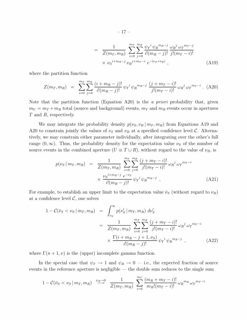
Page 17
– 17 –
=1
Z(mT , mR)
mT∑
i=0
mR∑
j=0
ψTi ψR
mR−j
i!(mR − j)!
ωRj ωT
mT −j
j!(mT − i)!
× νSi+mR−j νB
j+mT−i e−(νS+νB) , (A19)
where the partition function
Z(mT , mR) =
mT∑
i=0
mR∑
j=0
(i+mR − j)!
i!(mR − j)!ψT
i ψRmR−j (j +mT − i)!
j!(mT − i)!ωR
j ωTmT −i . (A20)
Note that the partition function (Equation A20) is the a priori probability that, given
mU = mT +mR total (source and background) events, mT and mR events occur in apertures
T and R, respectively.
We may integrate the probability density p(νS, νB |mT , mR) from Equations A19 and
A20 to constrain jointly the values of νS and νB at a specified confidence level C. Alterna-
tively, we may constrain either parameter individually, after integrating over the other’s full
range (0,∞). Thus, the probability density for the expectation value νS of the number of
source events in the combined aperture (U ≡ T ∪R), without regard to the value of νB, is
p(νS |mT , mR) =1
Z(mT , mR)
mT∑
i=0
mR∑
j=0
(j +mT − i)!
j!(mT − i)!ωR
j ωTmT −i
×νS
i+mR−j e−νS
i!(mR − j)!ψT
i ψRmR−j , (A21)
For example, to establish an upper limit to the expectation value νS (without regard to νB)
at a confidence level C, one solves
1 − C(νS < νS |mT , mR) =
∫ ∞
νS
p(ν ′S |mT , mR) dν ′S
=1
Z(mT , mR)
mT∑
i=0
mR∑
j=0
(j +mT − i)!
j!(mT − i)!ωR
j ωTmT −i
×Γ(i+mR − j + 1, νS)
i!(mR − j)!ψT
i ψRmR−j , (A22)
where Γ(n+ 1, ν) is the (upper) incomplete gamma function.
In the special case that ψT → 1 and ψR → 0 — i.e., the expected fraction of source
events in the reference aperture is negligible — the double sum reduces to the single sum
1 − C(νS < νS |mT , mR)ψR→0−→
1
Z(mT , mR)
mT∑
i=0
(mR +mT − i)!
mR!(mT − i)!ωR
mR ωTmT −i
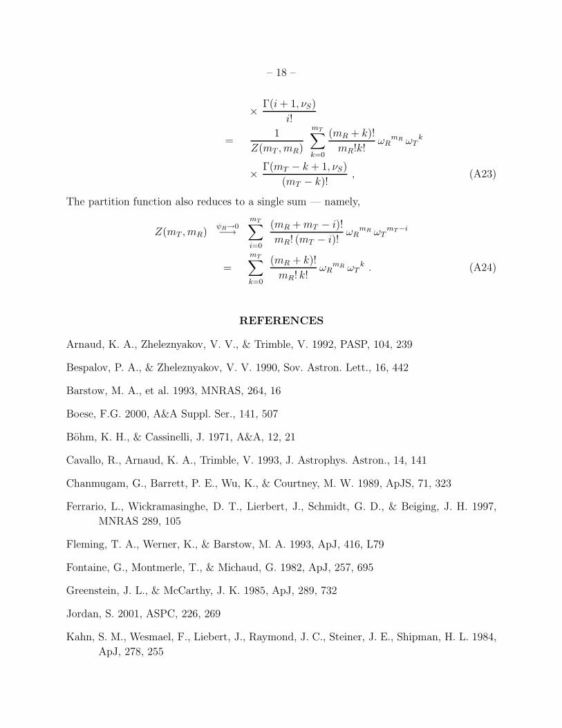
Page 18
– 18 –
×Γ(i+ 1, νS)
i!
=1
Z(mT , mR)
mT∑
k=0
(mR + k)!
mR!k!ωR
mR ωTk
×Γ(mT − k + 1, νS)
(mT − k)!, (A23)
The partition function also reduces to a single sum — namely,
Z(mT , mR)ψR→0−→
mT∑
i=0
(mR +mT − i)!
mR! (mT − i)!ωR
mR ωTmT −i
=
mT∑
k=0
(mR + k)!
mR! k!ωR
mR ωTk . (A24)
REFERENCES
Arnaud, K. A., Zheleznyakov, V. V., & Trimble, V. 1992, PASP, 104, 239
Bespalov, P. A., & Zheleznyakov, V. V. 1990, Sov. Astron. Lett., 16, 442
Barstow, M. A., et al. 1993, MNRAS, 264, 16
Boese, F.G. 2000, A&A Suppl. Ser., 141, 507
Bohm, K. H., & Cassinelli, J. 1971, A&A, 12, 21
Cavallo, R., Arnaud, K. A., Trimble, V. 1993, J. Astrophys. Astron., 14, 141
Chanmugam, G., Barrett, P. E., Wu, K., & Courtney, M. W. 1989, ApJS, 71, 323
Ferrario, L., Wickramasinghe, D. T., Lierbert, J., Schmidt, G. D., & Beiging, J. H. 1997,
MNRAS 289, 105
Fleming, T. A., Werner, K., & Barstow, M. A. 1993, ApJ, 416, L79
Fontaine, G., Montmerle, T., & Michaud, G. 1982, ApJ, 257, 695
Greenstein, J. L., & McCarthy, J. K. 1985, ApJ, 289, 732
Jordan, S. 2001, ASPC, 226, 269
Kahn, S. M., Wesmael, F., Liebert, J., Raymond, J. C., Steiner, J. E., Shipman, H. L. 1984,
ApJ, 278, 255
Page 19
– 19 –
Kawaler, S., Sekii, T., & Gough, D., 1999, ApJ, 516, 349
Kidder, K. M., Holberg, J. B., Barstow, M. A., Tweedy, R. W., & Wesmael, F. 1992, ApJ,
394, 288
Koester, D. 2002, A&A Rev., 11, 33
Koester, D., Beuermann, K., Thomas, H.-C., Graser, U., Giommi, P., & Tagliaferri, G. 1990,
A&A, 239, 260
Kraft, R. P., Burrows, D. N. & Nousek, J. A. 1991, ApJ, 374, 344
Li, J., Wickramasinghe, D. T., Ferrario, L. 1998, ApJ, 503, L151
McCook, G. P., & Sion, E. M. 1999, ApJS, 121, 1
Mermilliod, J.-C., & Mermilliod, M. 1994, Catalog of Mean UBV Data on Stars (New York:
Springer-Verlag)
Mewe, R., Heise, J., Gronenschild, E. H. B. M., Brinkman, A. C., Schrijver, J., & den
Boggende, A. J. F., 1975, Nature, 256, 711
Monet, D. G., et al. 2003, AJ,125, 984
Musielak, Z. E. 1987, ApJ, 322, 234
Musielak, Z. E., & Fontenla, J. M. 1989, ApJ, 346, 435
Musielak, Z. E., Porter, J. G., & Davis, J. M., 1995, ApJ, 453, L33
Musielak, Z.E., Noble, M., Porter, J. G. & Winget, D. E. 2003, ApJ, 593, 481
Musielak, Z. E., Winget, D. E., & Montgomery, M. H. 2005, ApJ, 630, 506
Ochsenbein, F., Bauer P., & Marcout, J. 2000, A&AS, 143, 221
Paerels, F. B. S., & Heise, J. 1989, ApJ, 339, 1000
Petre, R., Shipman, H. L., & Canizares, C. R. 1986, ApJ, 304, 356
Provencal, J. L., Shipman, H. L., & MacDonald, J. 2005, ApJ, 627, 418
Schmidt, G. D., & Smith, P. S. 1995, ApJ, 448, 305
Serber, A. V. 1990, Sov. Astron., 34, 291
Page 20
– 20 –
Shipman, H. L. 1976, ApJ, 206, L67
Skrutskie, M. F., et al. 2006, AJ, 131, 1163
Tennant, A. F. 2006, AJ, 132, 1372
Thomas, J. H., Markiel, J. A., & Van Horn, H. M. 1995, ApJ, 453, 403
van Altena, W. F., Lee, J. T., & Hoffleit, E. D. 1995, The General Catalogue of Trigonometric
Stellar Parallaxes, (4th ed.; New Haven CT: Yale University Observatory)
Wesmael, F., Auer, L. H., Van Horn, H. M., & Savedoff, M. P. 1980, ApJS, 43, 159
Winget, D. E. et al., 1994, ApJ, 430, 839
Zheleznyakov, V. V., Koryagin, S. A., & Serber, A. V. 2004, Astron. Reports, 31, 143
Zheleznyakov, V. V., & Litvinchuk, A. A. 1984, Ap&SS, 105, 73
Zheleznyakov, V. V., Serber, A. V., & Kuijpers, J. 1996, A&A, 308, 465
This preprint was prepared with the AAS LATEX macros v5.2.
Page 21
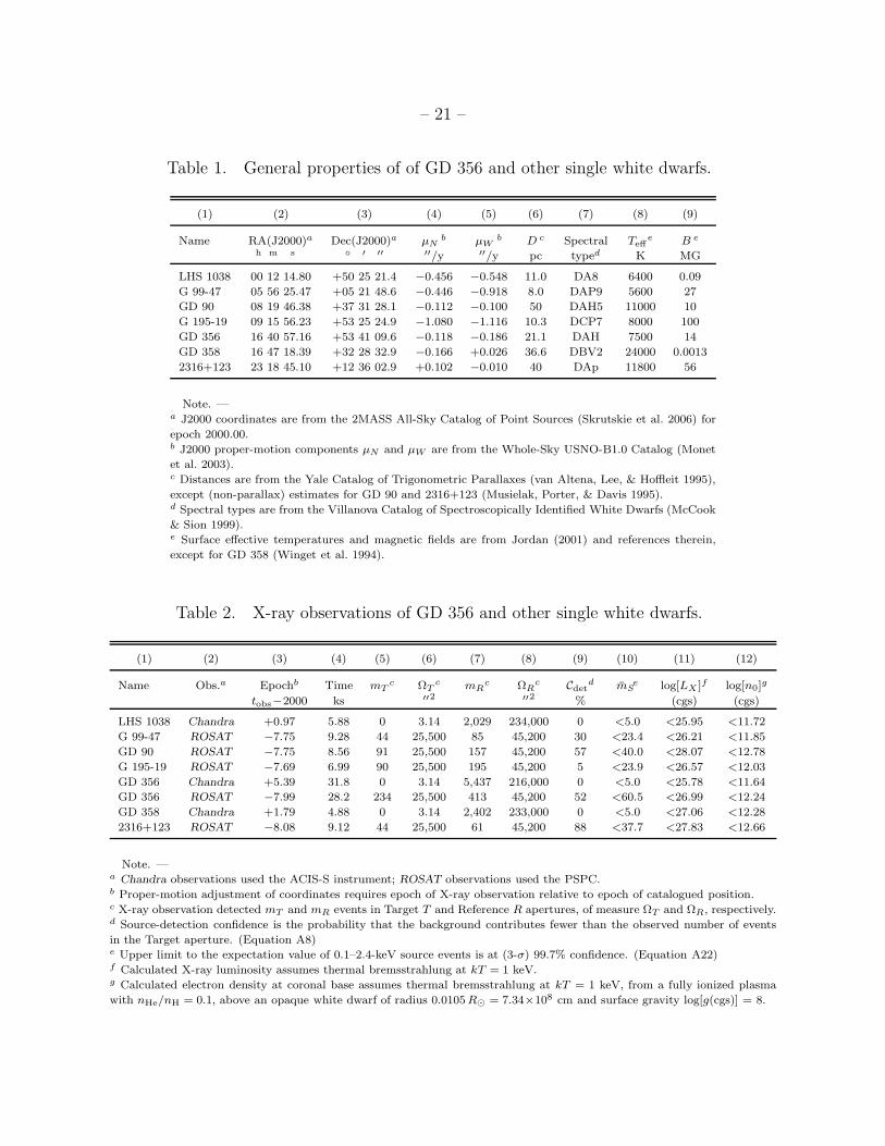
– 21 –
Table 1. General properties of of GD 356 and other single white dwarfs.
(1) (2) (3) (4) (5) (6) (7) (8) (9)
Name RA(J2000)a Dec(J2000)a µNb µW
b D c Spectral Teffe B e
h m s ′ ′′ ′′/y ′′/y pc typed K MG
LHS 1038 00 12 14.80 +50 25 21.4 −0.456 −0.548 11.0 DA8 6400 0.09
G 99-47 05 56 25.47 +05 21 48.6 −0.446 −0.918 8.0 DAP9 5600 27
GD 90 08 19 46.38 +37 31 28.1 −0.112 −0.100 50 DAH5 11000 10
G 195-19 09 15 56.23 +53 25 24.9 −1.080 −1.116 10.3 DCP7 8000 100
GD 356 16 40 57.16 +53 41 09.6 −0.118 −0.186 21.1 DAH 7500 14
GD 358 16 47 18.39 +32 28 32.9 −0.166 +0.026 36.6 DBV2 24000 0.0013
2316+123 23 18 45.10 +12 36 02.9 +0.102 −0.010 40 DAp 11800 56
Note. —a J2000 coordinates are from the 2MASS All-Sky Catalog of Point Sources (Skrutskie et al. 2006) for
epoch 2000.00.b J2000 proper-motion components µN and µW are from the Whole-Sky USNO-B1.0 Catalog (Monet
et al. 2003).c Distances are from the Yale Catalog of Trigonometric Parallaxes (van Altena, Lee, & Hoffleit 1995),
except (non-parallax) estimates for GD 90 and 2316+123 (Musielak, Porter, & Davis 1995).d Spectral types are from the Villanova Catalog of Spectroscopically Identified White Dwarfs (McCook
& Sion 1999).e Surface effective temperatures and magnetic fields are from Jordan (2001) and references therein,
except for GD 358 (Winget et al. 1994).
Table 2. X-ray observations of GD 356 and other single white dwarfs.
(1) (2) (3) (4) (5) (6) (7) (8) (9) (10) (11) (12)
Name Obs.a Epochb Time mTc ΩT
c mRc ΩR
c Cdetd mS
e log[LX ]f log[n0]g
tobs−2000 ks ′′2 ′′2 % (cgs) (cgs)
LHS 1038 Chandra +0.97 5.88 0 3.14 2,029 234,000 0 <5.0 <25.95 <11.72
G 99-47 ROSAT −7.75 9.28 44 25,500 85 45,200 30 <23.4 <26.21 <11.85
GD 90 ROSAT −7.75 8.56 91 25,500 157 45,200 57 <40.0 <28.07 <12.78
G 195-19 ROSAT −7.69 6.99 90 25,500 195 45,200 5 <23.9 <26.57 <12.03
GD 356 Chandra +5.39 31.8 0 3.14 5,437 216,000 0 <5.0 <25.78 <11.64
GD 356 ROSAT −7.99 28.2 234 25,500 413 45,200 52 <60.5 <26.99 <12.24
GD 358 Chandra +1.79 4.88 0 3.14 2,402 233,000 0 <5.0 <27.06 <12.28
2316+123 ROSAT −8.08 9.12 44 25,500 61 45,200 88 <37.7 <27.83 <12.66
Note. —a Chandra observations used the ACIS-S instrument; ROSAT observations used the PSPC.b Proper-motion adjustment of coordinates requires epoch of X-ray observation relative to epoch of catalogued position.c X-ray observation detected mT and mR events in Target T and Reference R apertures, of measure ΩT and ΩR, respectively.d Source-detection confidence is the probability that the background contributes fewer than the observed number of events
in the Target aperture. (Equation A8)e Upper limit to the expectation value of 0.1–2.4-keV source events is at (3-σ) 99.7% confidence. (Equation A22)f Calculated X-ray luminosity assumes thermal bremsstrahlung at kT = 1 keV.g Calculated electron density at coronal base assumes thermal bremsstrahlung at kT = 1 keV, from a fully ionized plasma
with nHe/nH = 0.1, above an opaque white dwarf of radius 0.0105R⊙ = 7.34×108 cm and surface gravity log[g(cgs)] = 8.
Page 22
– 22 –
Table 3. Chandra-detected sources in the GD-356 field.
(1) (2) (3) (4) (5) (6)
Source RA(J2000) Dec(J2000) θexta mD
b θ99c
h m s ′ ′′ ′′ ′′
1 16 40 45.029 +53 44 47.38 2.7 8.9 1.25
2 16 40 45.299 +53 45 13.15 3.1 13.6 1.18
3 16 40 53.706 +53 44 42.50 2.4 9.2 1.15
4 16 40 55.545 +53 40 25.24 1.3 22.0 0.69
5 16 40 56.104 +53 39 18.33 1.7 25.9 0.73
6 16 40 59.258 +53 41 59.41 1.2 36.4 0.66
7 16 41 00.438 +53 42 03.31 1.3 10.2 0.78
8 16 41 04.242 +53 40 20.98 1.6 7.3 0.94
9 16 41 05.997 +53 43 18.82 2.0 21.0 0.80
10 16 41 06.757 +53 37 52.85 3.3 30.6 0.94
11 16 41 07.650 +53 45 27.75 3.7 17.8 1.23
12 16 41 10.745 +53 44 36.43 3.2 16.5 1.13
13 16 41 13.050 +53 41 57.24 2.2 12.9 0.97
14 16 41 14.806 +53 41 41.18 2.4 12.6 1.02
15 16 41 15.481 +53 44 10.91 3.4 4559.0 0.61
16 16 41 16.876 +53 42 56.29 2.9 118.6 0.69
17 16 41 19.134 +53 44 11.29 3.9 32.1 1.03
18 16 41 21.033 +53 40 54.25 3.3 17.6 1.13
19 16 41 24.066 +53 41 48.86 3.8 8.2 1.71
20 16 41 30.445 +53 41 18.79 5.0 27.8 1.30
21 16 41 32.519 +53 36 40.09 8.4 17.8 2.49
22 16 41 33.184 +53 43 05.51 5.9 12.7 2.10
23 16 41 37.639 +53 39 57.65 6.9 8.5 2.93
Note. —a The extraction radius demarks the detect cell for collecting X-ray
counts.b An ACIS-S3 observation (ObsID 4484) acquired these detect-cell
counts in 31.8 ks.c This radius encloses the true position of the detected source at
99% confidence.
Page 23
– 23 –
Table 4. Chandra-detected sources in the LHS-1038 field.
(1) (2) (3) (4) (5) (6)
Source RA(J2000) Dec(J2000) θexta mD
b θ99c
h m s ′ ′′ ′′ ′′
1 0 12 05.742 +50 28 17.79 2.8 11.3 1.16
2 0 12 08.128 +50 30 16.70 4.6 10.1 1.86
3 0 12 10.118 +50 28 30.63 2.7 60.9 0.73
4 0 12 31.360 +50 32 16.93 8.1 35.5 1.75
Note. —a The extraction radius demarks the detect cell for collecting X-
ray counts.b An ACIS-S3 observation (ObsID 1864) acquired these detect-
cell counts in 5.88 ks.c This radius encloses the true position of the detected source at
99% confidence.
Table 5. Chandra-detected sources in the GD-358 field.
(1) (2) (3) (4) (5) (6)
Source RA(J2000) Dec(J2000) θexta mD
b θ99c
h m s ′ ′′ ′′ ′′
1 16 46 55.620 +32 29 49.17 4.8 6.9 2.29
2 16 46 58.650 +32 29 30.20 3.9 9.6 1.64
3 16 47 07.418 +32 30 50.62 3.0 25.1 0.95
4 16 47 08.044 +32 25 17.23 2.7 17.2 0.99
5 16 47 13.515 +32 32 03.03 3.5 20.6 1.12
6 16 47 17.610 +32 33 15.56 4.8 25.3 1.31
7 16 47 18.628 +32 27 51.63 1.1 51.1 0.63
8 16 47 18.645 +32 29 16.22 1.4 13.3 0.76
9 16 47 26.652 +32 27 30.17 1.4 8.4 0.85
10 16 47 27.949 +32 27 37.51 1.5 13.0 0.80
Note. —a The extraction radius demarks the detect cell for collecting X-ray
counts.b An ACIS-S3 observation (ObsID 1865) acquired these detect-cell
counts in 4.88 ks.c This radius encloses the true position of the detected source at
99% confidence.
Page 24
– 24 –
Fig. 1.— The 99.7%-confidence upper limits to total X-ray luminosity versus temperature
(upper panel) for bremsstrahlung and (lower panel) for MEKAL models. From lowest to
highest, limits based upon Chandra data (solid lines) are for GD 356, LHS 1038, and GD 358;
those based upon ROSAT data (× markers) are for G 99-47, G 195-19, GD 356, 2316+123,
and GD 90.
Page 25
– 25 –
Fig. 2.— The 99.7%-confidence upper limits to coronal electron density versus temperature
(upper panel) for bremsstrahlung and (lower panel) for MEKAL models. From lowest to
highest, limits based upon Chandra data (solid lines) are for GD 356, LHS 1038, and GD 358;
those based upon ROSAT data (× markers) are for G 99-47, G 195-19, GD 356, 2316+123,
and GD 90.
Page 26
– 26 –
Fig. 3.— Emergent cyclotron spectrum from a hypothesized hot corona around GD 356, in
comparison to a 7840-K photospheric spectrum (dashed line) and photometric data (square
markers). Calculations assume a 15-MG field at a mean viewing angle θ = arctan(0.5) =
26.6 and coronal parameters discussed in the text (§4), for a (coronal-base) electron density
n0 = 1×1011 cm−3 and temperature T = 1.5 keV (solid line) or 1.0 keV (dotted line).
Page 27
– 27 –
Fig. 4.— Contributors to the luminosity of a hypothetical corona around the magnetic white
dwarf GD 356, in comparison to its photospheric luminosity (horizontal, thin dashed line).
Solid lines denote the thermal cyclotron luminosity for B = 15 MG and kT = 0.125, 0.25, 0.5,
1.0, and 2.0 keV, in increasing thickness. Dotted lines denote the thermal-bremsstrahlung
luminosity for the same set of coronal temperatures.