706


ftoc.qxd 10/15/09 12:38 PM Page xviii

• Studentsachieveconceptmasteryinarich,structuredenvironmentthat’savailable24/7
From multiple study paths, to self-assessment, to a wealth of interactive
visual and audio resources, WileyPLUS gives you everything you need to
personalize the teaching and learning experience.
WithWileyPLUS:
»F indout how toMake It YourS »
This online teaching and learning environment integrates the entire digital textbook with the most effective instructor and student resources to fit every learning style.
• Instructorspersonalizeandmanagetheircoursemoreeffectivelywithassessment,assignments,gradetracking,andmore
•managetimebetter
•studysmarter
•savemoney
www.wileyplus.com

MakeItYourS!
aLL The heLP, reSoUrceS, and PerSonaL SUPPorTyoU and yoUr STUdenTS need!
technicalSupport24/7FaQs,onlinechat,andphonesupport
www.wileyplus.com/support
Studentsupportfromanexperiencedstudentuser
askyourlocalrepresentativefordetails!
YourWileyPLUSaccountManager
trainingandimplementationsupportwww.wileyplus.com/accountmanager
Collaboratewithyourcolleagues,findamentor,attendvirtualandlive
events,andviewresourceswww.WhereFacultyconnect.com
Pre-loaded,ready-to-useassignmentsandpresentations
www.wiley.com/college/quickstart
2-Minutetutorialsandalloftheresourcesyou&yourstudentsneedtogetstartedwww.wileyplus.com/firstday

StatisticsPrinciples and Methods
SIXTH EDITION
Richard A. JohnsonUniversity of Wisconsin at Madison
Gouri K. Bhattacharyya
John Wiley & Sons, Inc.
ffirs.qxd 10/15/09 12:24 PM Page iii

Vice President & Executive Publisher Laurie RosatoneProject Editor Ellen KeohaneSenior Development Editor Anne Scanlan-RohrerProduction Manager Dorothy SinclairSenior Production Editor Valerie A. VargasMarketing Manager Sarah DavisCreative Director Harry NolanDesign Director Jeof VitaProduction Management Services mb editorial services Photo Editor Sheena GoldsteinEditorial Assistant Beth PearsonMedia Editor Melissa EdwardsCover Photo Credit Gallo Images-Hein von
Horsten/Getty Images, Inc.Cover Designer Celia Wiley
This book was set in 10/12 Berling by Laserwords Private Limited, India and printed and bound by RR Donnelley-Crawsfordville. The cover was printed by RR Donnelley-Crawsfordville.
Copyright © 2010, 2006 John Wiley & Sons, Inc. All rights reserved. No part of this publicationmay be reproduced, stored in a retrieval system or transmitted in any form or by any means,electronic, mechanical, photocopying, recording, scanning or otherwise, except as permitted under Sections 107 or 108 of the 1976 United States Copyright Act, without either the prior written permission of the Publisher, or authorization through payment of the appropriate per-copyfee to the Copyright Clearance Center, Inc. 222 Rosewood Drive, Danvers, MA 01923, websitewww.copyright.com. Requests to the Publisher for permission should be addressed to the Permissions Department, John Wiley & Sons, Inc., 111 River Street, Hoboken, NJ 07030-5774,(201)748-6011, fax (201)748-6008, website http://www.wiley.com/go/permissions.
Evaluation copies are provided to qualified academics and professionals for review purposes only,for use in their courses during the next academic year. These copies are licensed and may not be sold or transferred to a third party. Upon completion of the review period, please return the evaluation copy to Wiley. Return instructions and a free of charge return shipping label are available at www.wiley.com/go/returnlabel. Outside of the United States, please contact your local representative.
ISBN-13 978-0-470-40927-5
Printed in the United States of America
10 9 8 7 6 5 4 3 2 1
ffirs.qxd 10/15/09 12:24 PM Page iv

Preface
THE NATURE OF THE BOOK
Conclusions, decisions, and actions that are data driven predominate in today'sworld. Statistics—the subject of data analysis and data-based reasoning—is neces-sarily playing a vital role in virtually all professions. Some familiarity with this sub-ject is now an essential component of any college education. Yet, pressures to ac-commodate a growing list of academic requirements often necessitate that thisexposure be brief. Keeping these conditions in mind, we have written this book toprovide students with a first exposure to the powerful ideas of modern statistics. Itpresents the key statistical concepts and the most commonly applied methods ofstatistical analysis. Moreover, to keep it accessible to freshmen and sophomoresfrom a wide range of disciplines, we have avoided mathematical derivations. Theyusually pose a stumbling block to learning the essentials in a short period of time.
This book is intended for students who do not have a strong background inmathematics but seek to learn the basic ideas of statistics and their applicationin a variety of practical settings. The core material of this book is common to al-most all first courses in statistics and is designed to be covered well within aone-semester course in introductory statistics for freshmen–seniors. It is supple-mented with some additional special-topics chapters.
ORIENTATION
The topics treated in this text are, by and large, the ones typically covered in anintroductory statistics course. They span three major areas: (i) descriptive statis-tics, which deals with summarization and description of data; (ii) ideas of proba-bility and an understanding of the manner in which sample-to-sample variationinfluences our conclusions; and (iii) a collection of statistical methods for analyz-ing the types of data that are of common occurrence. However, it is the treatmentof these topics that makes the text distinctive. Throughout, we have endeavoredto give clear and concise explanations of the concepts and important statisticalterminology and methods. By means of good motivation, sound explanations, andan abundance of illustrations given in a real-world context, it emphasizes morethan just a superficial understanding.
v
fpref.qxd 10/15/09 12:37 PM Page v

Each statistical concept or method is motivated by setting out its goal and thenfocusing on an example to further elaborate important aspects and to illustrate itsapplication. The subsequent discussion is not only limited to showing how amethod works but includes an explanation of the why. Even without recourse tomathematics, we are able to make the reader aware of possible pitfalls in the statis-tical analysis. Students can gain a proper appreciation of statistics only when theyare provided with a careful explanation of the underlying logic. Without this un-derstanding, a learning of elementary statistics is bound to be rote and transient.
When describing the various methods of statistical analysis, the reader iscontinually reminded that the validity of a statistical inference is contingentupon certain model assumptions. Misleading conclusions may result when theseassumptions are violated. We feel that the teaching of statistics, even at an intro-ductory level, should not be limited to the prescription of methods. Studentsshould be encouraged to develop a critical attitude in applying the methods andto be cautious when interpreting the results. This attitude is especially impor-tant in the study of relationship among variables, which is perhaps the mostwidely used (and also abused) area of statistics. In addition to discussing infer-ence procedures in this context, we have particularly stressed critical examina-tion of the model assumptions and careful interpretation of the conclusions.
SPECIAL FEATURES
1. Crucial elements are boxed to highlight important concepts and meth-ods. These boxes provide an ongoing summary of the important itemsessential for learning statistics. At the end of each chapter, all of its keyideas and formulas are summarized.
2. A rich collection of examples and exercises is included. These aredrawn from a large variety of real-life settings. In fact, many data setsstem from genuine experiments, surveys, or reports.
3. Exercises are provided at the end of each major section. These provide thereader with the opportunity to practice the ideas just learned. Occasion-ally, they supplement some points raised in the text. A larger collection ofexercises appears at the end of a chapter. The starred problems are rela-tively difficult and suited to the more mathematically competent student.
4. Using Statistics Wisely, a feature at the end of each chapter, providesimportant guidelines for the appropriate use of the statistical proce-dures presented in the chapter.
5. Statistics in Context sections, in four of the beginning chapters, each describe an important statistical application where a statistical approachto understanding variation is vital. These extended examples reveal, earlyon in the course, the value of understanding the subject of statistics.
6. P–values are emphasized in examples concerning tests of hypotheses.Graphs giving the relevant normal or t density curve, rejection region,and P–value are presented.
vi PREFACE
fpref.qxd 10/15/09 12:37 PM Page vi

7. Regression analysis is a primary statistical technique so we provide amore thorough coverage of the topic than is usual at this level. The ba-sics of regression are introduced in Chapter 11, whereas Chapter 12stretches the discussion to several issues of practical importance. Theseinclude methods of model checking, handling nonlinear relations, andmultiple regression analysis. Complex formulas and calculations are ju-diciously replaced by computer output so the main ideas can be learnedand appreciated with a minimum of stress.
8. Integrated Technology, at the end of most chapters, details the steps for us-ing MINITAB, EXCEL, and TI-84 calculator. With this presentation avail-able, with few exceptions, only computer output is needed in the text.Software packages remove much of the drudgery of hand calculationand they allow students to work with larger data sets where patterns aremore pronounced. Some computer exercises are included in all chap-ters where relevant.
9. Convenient Electronic Data Bank at the end of the book contains a sub-stantial collection of data. These data sets, together with numerous oth-ers throughout the book, allow for considerable flexibility in the choicebetween concept-orientated and applications-orientated exercises. TheData Bank and the other larger data sets are available for download onthe accompanying Web site located at www.wiley.com/college/johnson.
10. Technical Appendix A presents a few statistical facts of a mathematicalnature. These are separated from the main text so that they can be leftout if the instructor so desires.
ABOUT THE SIXTH EDITION
The sixth edition of STATISTICS—Principles and Methods maintains the objec-tives and level of presentation of the earlier editions. The goals are the develop-ing (i) of an understanding of the reasonings by which findings from sampledata can be extended to general conclusions and (ii) a familiarity with somebasic statistical methods. There are numerous data sets and computer outputswhich give an appreciation of the role of the computer in modern data analysis.
Clear and concise explanations introduce the concepts and important sta-tistical terminology and methods. Real-life settings are used to motivate thestatistical ideas and well organized discussions proceed to cover statisticalmethods with heavy emphasis on examples. The sixth edition enhances thesespecial features. The major improvements are:
Bayes’ Theorem. A new section is added to Chapter 4 to highlight the rea-soning underlying Bayes’s theorem and to present applications.
Approximate t. A new subsection is added to Chapter 7, which describesthe approximate two sample t statistic that is now pervasive in statistical soft-ware programs. For normal distributions, with unequal variances, this has be-come the preferred approach.
1
PREFACE vii
Commands and the worksheets with data sets pertain to EXCEL 2003.1
fpref.qxd 10/15/09 12:37 PM Page vii

New Examples. A substantial number of new examples are included, espe-cially in the core chapters, Chapter 11 on regression, and Chapter 13 on contin-gency tables.
More Data-Based Exercises. Most of the new exercises are keyed to newdata-based examples in the text. New data are also presented in the exercises.Other new exercises are based on the credit card use and opinion data that areadded to the data bank.
New Exercises. Numerous new exercises provide practice on understandingthe concepts and others address computations. These new exercises, which aug-ment the already rich collection, are placed in real-life settings to help promotea greater appreciation of the wide span of applicability of statistical methods.
ORGANIZATION
This book is organized into fifteen chapters, an optional technical appendix(Appendix A), and a collection of tables (Appendix B). Although designed for aone-semester or a two-quarter course, it is enriched with ample additional mate-rial to allow the instructor some choices of topics. Beyond Chapter 1, which setsthe theme of statistics and distinguishes population and sample, the subjectmatter could be classified as follows:
Topic Chapter
Descriptive study of data 2, 3
Probability and distributions 4, 5, 6
Sampling variability 7
Core ideas and methods of statistical inference 8, 9, 10
Special topics of statistical inference 11, 12, 13, 14, 15
We regard Chapters 1 to 10 as constituting the core material of an introduc-tory statistics course, with the exception of the starred sections in Chapter 6. Al-though this material is just about enough for a one-semester course, manyinstructors may wish to eliminate some sections in order to cover the basics of re-gression analysis in Chapter 11. This is most conveniently done by initially skippingChapter 3 and then taking up only those portions that are linked to Chapter 11.Also, instead of a thorough coverage of probability that is provided in Chapter 4,the later sections of that chapter may receive a lighter coverage.
SUPPLEMENTS
Instructor’s Solution Manual. (ISBN 978-0-470-53519-6) This manual con-tains complete solutions to all exercises.
viii PREFACE
fpref.qxd 10/15/09 12:37 PM Page viii

Test Bank. (Available on the accompanying website: www.wiley.com/college/johnson) Contains a large number of additional questions for each chapter.
Student Solutions Manual. (ISBN 978-0-470-53521-9) This manual con-tains complete solutions to all odd-numbered exercises.
Electronic Data Bank. (Available on the accompanying website: www.wiley.com/college/johnson) Contains interesting data sets used in the text but thatcan be used to perform additional analyses with statistical software packages.
WileyPLUS. This powerful online tool provides a completely integrated suiteof teaching and learning resources in one easy-to-use website. WileyPLUS offersan online assessment system with full gradebook capabilities and algorithmicallygenerated skill building questions. This online teaching and learning environmentalso integrates the entire digital textbook. To view a demo of WileyPLUS, contactyour local Wiley Sales Representative or visit: www.wiley.com/college/wileyplus.
ACKNOWLEDGMENTS
We thank Minitab (State College, Pa.) and the SAS Institute (Cary, N.C.) for per-mission to include commands and output from their software packages. A specialthanks to K. T. Wu and Kam Tsui for many helpful suggestions and comments onearlier editions. We also thank all those who have contributed the data sets whichenrich the presentation and all those who reviewed the previous editions. Thefollowing people gave their careful attention to this edition:
Hongshik Ahn, Stony Brook UniversityPrasanta Basak, Penn State University AltoonaAndrea Boito, Penn State University AltoonaPatricia M. Buchanan, Penn State UniversityNural Chowdhury, University of SaskatchewanS. Abdul Fazal, California State University StanislausChristian K. Hansen, Eastern Washington UniversitySusan Kay Herring, Sonoma State UniversityHui-Kuang Hsieh, University of Massachusetts AmherstHira L. Koul, Michigan State UniversityMelanie Martin, California State University StanislausMark McKibben, Goucher CollegeCharles H. Morgan, Jr., Lock Haven University of PennsylvaniaPerpetua Lynne Nielsen, Brigham Young UniversityAshish Kumar Srivastava, St. Louis UniversityJames Stamey, Baylor UniversityMasoud Tabatabai, Penn State University HarrisburgJed W. Utsinger, Ohio UniversityR. Patrick Vernon, Rhodes College
PREFACE ix
fpref.qxd 10/15/09 12:37 PM Page ix

Roumen Vesselinov, University of South CarolinaVladimir Vinogradov, Ohio UniversityA. G. Warrack, North Carolina A&T State University
Richard A. JohnsonGouri K. Bhattacharyya
x PREFACE
fpref.qxd 10/15/09 12:37 PM Page x

Contents
1 INTRODUCTION 1
1 What Is Statistics? 32 Statistics in Our Everyday Life 33 Statistics in Aid of Scientific Inquiry 54 Two Basic Concepts—Population and Sample 85 The Purposeful Collection of Data 146 Statistics in Context 157 Objectives of Statistics 178 Using Statistics Wisely 189 Key Ideas 18
10 Review Exercises 19
2 ORGANIZATION AND DESCRIPTION OF DATA 21
1 Introduction 232 Main Types of Data 233 Describing Data by Tables and Graphs 24
3.1 Categorical Data 243.2 Discrete Data 283.3 Data on a Continuous Variable 29
4 Measures of Center 405 Measures of Variation 486 Checking the Stability of the Observations over Time 607 More on Graphics 648 Statistics in Context 669 Using Statistics Wisely 68
10 Key Ideas and Formulas 6811 Technology 7012 Review Exercises 73
xi
ftoc.qxd 10/15/09 12:38 PM Page xi

xii CONTENTS
3 DESCRIPTIVE STUDY OF BIVARIATE DATA 81
1 Introduction 832 Summarization of Bivariate Categorical Data 833 A Designed Experiment for Making a Comparison 884 Scatter Diagram of Bivariate Measurement Data 905 The Correlation Coefficient—A Measure of Linear Relation 936 Prediction of One Variable from Another (Linear Regression) 1047 Using Statistics Wisely 1098 Key Ideas and Formulas 1099 Technology 110
10 Review Exercises 111
4 PROBABILITY 115
1 Introduction 1172 Probability of an Event 1183 Methods of Assigning Probability 124
3.1 Equally Likely Elementary Outcomes—The Uniform Probability Model 124
3.2 Probability As the Long-Run Relative Frequency 1264 Event Relations and Two Laws of Probability 1325 Conditional Probability and Independence 1416 Bayes’ Theorem 1407 Random Sampling from a Finite Population 1558 Using Statistics Wisely 1629 Key Ideas and Formulas 162
10 Technology 16411 Review Exercises 165
5 PROBABILITY DISTRIBUTIONS 171
1 Introduction 1732 Random Variables 1733 Probability Distribution of a Discrete Random Variable 1764 Expectation (Mean) and Standard Deviation
of a Probability Distribution 1855 Successes and Failures—Bernoulli Trials 1936 The Binomial Distribution 1987 The Binomial Distribution in Context 2088 Using Statistics Wisely 2119 Key Ideas and Formulas 212
10 Technology 21311 Review Exercises 215
ftoc.qxd 10/15/09 12:38 PM Page xii

6 THE NORMAL DISTRIBUTION 221
1 Probability Model for a Continuous Random Variable 223
2 The Normal Distribution—Its General Features 2303 The Standard Normal Distribution 2334 Probability Calculations with Normal Distributions 2385 The Normal Approximation to the Binomial 242
*6 Checking the Plausibility of a Normal Model 248*7 Transforming Observations to Attain
Near Normality 2518 Using Statistics Wisely 2549 Key Ideas and Formulas 255
10 Technology 25611 Review Exercises 257
7 VARIATION IN REPEATED SAMPLES—SAMPLING DISTRIBUTIONS 263
1 Introduction 2652 The Sampling Distribution of a Statistic 2663 Distribution of the Sample Mean and
the Central Limit Theorem 2734 Statistics in Context 2855 Using Statistics Wisely 2896 Key Ideas and Formulas 2897 Review Exercises 2908 Class Projects 2929 Computer Project 293
8 DRAWING INFERENCES FROM LARGE SAMPLES 295
1 Introduction 2972 Point Estimation of a Population Mean 2993 Confidence Interval for a Population Mean 3054 Testing Hypotheses about a Population Mean 3145 Inferences about a Population Proportion 3296 Using Statistics Wisely 3377 Key Ideas and Formulas 3388 Technology 3409 Review Exercises 343
CONTENTS xiii
ftoc.qxd 10/15/09 12:38 PM Page xiii

xiv CONTENTS
9 SMALL-SAMPLE INFERENCES FOR NORMAL POPULATIONS 349
1 Introduction 3512 Student’s t Distribution 3513 Inferences about �—Small Sample Size 355
3.1 Confidence Interval for � 3553.2 Hypotheses Tests for � 358
4 Relationship between Tests and Confidence Intervals 3635 Inferences about the Standard Deviation �
(The Chi-Square Distribution) 3666 Robustness of Inference Procedures 3717 Using Statistics Wisely 3728 Key Ideas and Formulas 3739 Technology 375
10 Review Exercises 376
10 COMPARING TWO TREATMENTS 381
1 Introduction 3832 Independent Random Samples from Two Populations 3863 Large Samples Inference about Difference of Two Means 3884 Inferences from Small Samples: Normal Populations with
Equal Variances 3945 Inferences from Small Samples: Normal Populations with Unequal
Variances 4005.1 A Conservative t Test 4005.2 An Approximate t Test—Satterthwaite Correction 402
6 Randomization and Its Role in Inference 4077 Matched Pairs Comparisons 409
7.1 Inferences from a Large Number of Matched Pairs 4127.2 Inferences from a Small Number of Matched Pairs 4137.3 Randomization with Matched Pairs 416
8 Choosing between Independent Samples and a Matched Pairs Sample 4189 Comparing Two Population Proportions 420
10 Using Statistics Wisely 42611 Key Ideas and Formulas 42712 Technology 43113 Review Exercises 434
11 REGRESSION ANALYSIS—ISimple Linear Regression 439
1 Introduction 4412 Regression with a Single Predictor 443
ftoc.qxd 10/15/09 12:38 PM Page xiv

CONTENTS xv
3 A Straight-Line Regression Model 4464 The Method of Least Squares 4485 The Sampling Variability of the Least Squares Estimators—
Tools for Inference 4566 Important Inference Problems 458
6.1. Inference Concerning the Slope � 4586.2. Inference about the Intercept � 4606.3. Estimation of the Mean Response for a Specified x Value 4606.4. Prediction of a Single Response for a Specified x Value 463
7 The Strength of a Linear Relation 4718 Remarks about the Straight Line Model Assumptions 4769 Using Statistics Wisely 476
10 Key Ideas and Formulas 47711 Technology 48012 Review Exercises 481
12 REGRESSION ANALYSIS—IIMultiple Linear Regression and Other Topics 485
1 Introduction 4872 Nonlinear Relations and Linearizing Transformations 4873 Multiple Linear Regression 4914 Residual Plots to Check the Adequacy of a Statistical Model 5035 Using Statistics Wisely 5076 Key Ideas and Formulas 5077 Technology 5088 Review Exercises 509
13 ANALYSIS OF CATEGORICAL DATA 513
1 Introduction 5152 Pearson’s Test for Goodness of Fit 5183 Contingency Table with One Margin Fixed
(Test of Homogeneity) 5224 Contingency Table with Neither Margin Fixed (Test of Independence) 5315 Using Statistics Wisely 5376 Key Ideas and Formulas 5377 Technology 5398 Review Exercises 540
14 ANALYSIS OF VARIANCE (ANOVA) 543
1 Introduction 5452 Comparison of Several Treatments—
The Completely Randomized Design 545
�2
0
1
ftoc.qxd 10/15/09 12:38 PM Page xv

xvi CONTENTS
3 Population Model and Inferences for a Completely Randomized Design 553
4 Simultaneous Confidence Intervals 5575 Graphical Diagnostics and Displays
to Supplement ANOVA 5616 Randomized Block Experiments
for Comparing k Treatments 5637 Using Statistics Wisely 5718 Key Ideas and Formulas 5729 Technology 573
10 Review Exercises 574
15 NONPARAMETRIC INFERENCE 577
1 Introduction 5792 The Wilcoxon Rank-Sum Test for Comparing
Two Treatments 5793 Matched Pairs Comparisons 5904 Measure of Correlation Based on Ranks 5995 Concluding Remarks 6036 Using Statistics Wisely 6047 Key Ideas and Formulas 6048 Technology 6059 Review Exercises 605
APPENDIX A1 SUMMATION NOTATION 609
APPENDIX A2 RULES FOR COUNTING 614
APPENDIX A3 EXPECTATION AND STANDARD DEVIATION—PROPERTIES 617
APPENDIX A4 THE EXPECTED VALUE AND STANDARD DEVIATION OF
_X 622
ftoc.qxd 10/15/09 12:38 PM Page xvi

APPENDIX B TABLES 624
Table 1 Random Digits 624Table 2 Cumulative Binomial Probabilities 627Table 3 Standard Normal Probabilities 634Table 4 Percentage Points of t Distributions 636Table 5 Percentage Points of Distributions 637Table 6 Percentage Points of F ( , ) Distributions 638Table 7 Selected Tail Probabilities for the Null Distribution of
Wilcoxon’s Rank-Sum Statistic 640Table 8 Selected Tail Probabilities for the Null Distribution
of Wilcoxon’s Signed-Rank Statistic 645
DATA BANK 647
ANSWERS TO SELECTED ODD-NUMBERED EXERCISES 665
INDEX 681
v2v1
�2
CONTENTS xvii
ftoc.qxd 10/15/09 12:38 PM Page xvii

ftoc.qxd 10/15/09 12:38 PM Page xviii

1. What Is Statistics?2. Statistics in Our Everyday Life3. Statistics in Aid of Scientific Inquiry4. Two Basic Concepts—Population and Sample5. The Purposeful Collection of Data6. Statistics in Context7. Objectives of Statistics8. Review Exercises
1
Introduction
c01.qxd 10/15/09 11:59 AM Page 1

Hometown fans attending today’s game are but a sample of the population of all localfootball fans. A self-selected sample may not be entirely representative of the populationon issues such as ticket price increases. Kiichiro Sato/ © AP/Wide World Photos
1These percentages are similar to those obtained by the ESPN Sports Poll, a service of TNS, in a2007 poll of over 27,000 fans.
Surveys Provide InformationAbout the Population
What is your favorite spectator sport?
Football 36.4%Baseball 12.7%Basketball 12.5%Other 38.4%
College and professional sports are combined in our summary.1 Clearly, footballis the most popular spectator sport. Actually, the National Football League byitself is more popular than baseball.
Until the mid 1960s, baseball was most popular according to similar surveys.Surveys, repeated at different times, can detect trends in opinion.
c01.qxd 10/15/09 11:59 AM Page 2

1. WHAT IS STATISTICS?
The word statistics originated from the Latin word “status,” meaning “state.” For along time, it was identified solely with the displays of data and charts pertainingto the economic, demographic, and political situations prevailing in a country.Even today, a major segment of the general public thinks of statistics as synony-mous with forbidding arrays of numbers and myriad graphs. This image is en-hanced by numerous government reports that contain a massive compilation ofnumbers and carry the word statistics in their titles: “Statistics of Farm Produc-tion,” “Statistics of Trade and Shipping,” “Labor Statistics,” to name a few. How-ever, gigantic advances during the twentieth century have enabled statistics togrow and assume its present importance as a discipline of data-based reasoning.Passive display of numbers and charts is now a minor aspect of statistics, andfew, if any, of today’s statisticians are engaged in the routine activities of tabula-tion and charting.
What, then, are the role and principal objectives of statistics as a scientificdiscipline? Stretching well beyond the confines of data display, statistics dealswith collecting informative data, interpreting these data, and drawing conclusionsabout a phenomenon under study. The scope of this subject naturally extends toall processes of acquiring knowledge that involve fact finding through collectionand examination of data. Opinion polls (surveys of households to study sociolog-ical, economic, or health-related issues), agricultural field experiments (with newseeds, pesticides, or farming equipment), clinical studies of vaccines, and cloudseeding for artificial rain production are just a few examples. The principles andmethodology of statistics are useful in answering questions such as, What kindand how much data need to be collected? How should we organize and interpretthe data? How can we analyze the data and draw conclusions? How do we assessthe strength of the conclusions and gauge their uncertainty?
2. STATISTICS IN OUR EVERYDAY LIFE 3
2. STATISTICS IN OUR EVERYDAY LIFE
Fact finding through the collection and interpretation of data is not confined to pro-fessional researchers. In our attempts to understand issues of environmental protec-tion, the state of unemployment, or the performance of competing football teams,numerical facts and figures need to be reviewed and interpreted. In our day-to-daylife, learning takes place through an often implicit analysis of factual information.
We are all familiar to some extent with reports in the news media on im-portant statistics.
Statistics as a subject provides a body of principles and methodology fordesigning the process of data collection, summarizing and interpretingthe data, and drawing conclusions or generalities.
c01.qxd 10/15/09 11:59 AM Page 3

Employment. Monthly, as part of the Current Population Survey, theBureau of Census collects information about employment status from a sample ofabout 65,000 households. Households are contacted on a rotating basis with three-fourths of the sample remaining the same for any two consecutive months.
The survey data are analyzed by the Bureau of Labor Statistics, which re-ports monthly unemployment rates. �
Cost of Living. The consumer price index (CPI) measures the cost of afixed market basket of over 400 goods and services. Each month, prices are ob-tained from a sample of over 18,000 retail stores that are distributed over 85metropolitan areas. These prices are then combined taking into account the rela-tive quantity of goods and services required by a hypothetical “1967 urban wageearner.” Let us not be concerned with the details of the sampling method andcalculations as these are quite intricate. They are, however, under close scrutinybecause of the importance to the hundreds of thousands of Americans whoseearnings or retirement benefits are tied to the CPI. �
Election time brings the pollsters into the limelight.
Gallup Poll. This, the best known of the national polls, produces esti-mates of the percentage of popular vote for each candidate based on interviewswith a minimum of 1500 adults. Beginning several months before the presiden-tial election, results are regularly published. These reports help predict winnersand track changes in voter preferences. �
Our sources of factual information range from individual experience to reportsin news media, government records, and articles in professional journals. As con-sumers of these reports, citizens need some idea of statistical reasoning to properlyinterpret the data and evaluate the conclusions. Statistical reasoning provides crite-ria for determining which conclusions are supported by the data and which are not.The credibility of conclusions also depends greatly on the use of statistical methodsat the data collection stage. Statistics provides a key ingredient for any systematicapproach to improve any type of process from manufacturing to service.
Quality and Productivity Improvement. In the past 30 years, theUnited States has faced increasing competition in the world marketplace. An in-ternational revolution in quality and productivity improvement has heightenedthe pressure on the U.S. economy. The ideas and teaching of W. Edwards Dem-ing helped rejuvenate Japan’s industry in the late 1940s and 1950s. In the 1980sand 1990s, Deming stressed to American executives that, in order to survive,they must mobilize their work force to make a continuing commitment to qual-ity improvement. His ideas have also been applied to government. The city ofMadison, WI, has implemented quality improvement projects in the police de-partment and in bus repair and scheduling. In each case, the project goal wasbetter service at less cost. Treating citizens as the customers of government ser-vices, the first step was to collect information from them in order to identify sit-uations that needed improvement. One end result was the strategic placementof a new police substation and a subsequent increase in the number of foot pa-trol persons to interact with the community.
4 CHAPTER 1/INTRODUCTION
c01.qxd 10/15/09 11:59 AM Page 4

Once a candidate project is selected for improvement, data must be col-lected to assess the current status and then more data collected on the effects ofpossible changes. At this stage, statistical skills in the collection and presentationof summaries are not only valuable but necessary for all participants.
In an industrial setting, statistical training for all employees—productionline and office workers, supervisors, and managers—is vital to the quality trans-formation of American industry. �
3. STATISTICS IN AID OF SCIENTIFIC INQUIRY
The phrase scientific inquiry refers to a systematic process of learning. A scien-tist sets the goal of an investigation, collects relevant factual information (ordata), analyzes the data, draws conclusions, and decides further courses of ac-tion. We briefly outline a few illustrative scenarios.
Training Programs. Training or teaching programs in many fields designedfor a specific type of clientele (college students, industrial workers, minority groups,physically handicapped people, retarded children, etc.) are continually monitored,evaluated, and modified to improve their usefulness to society. To learn about thecomparative effectiveness of different programs, it is essential to collect data on theachievement or growth of skill of the trainees at the completion of each program. �
Monitoring Advertising Claims. The public is constantly bombardedwith commercials that claim the superiority of one product brand in comparison toothers. When such comparisons are founded on sound experimental evidence, they
3. STATISTICS IN AID OF SCIENTIFIC INQUIRY 5
Statistical reasoning can guide the purposeful collection and analysis of data toward thecontinuous improvement of any process. © Andrew Sacks/Stone/Getty Images
c01.qxd 10/15/09 11:59 AM Page 5

serve to educate the consumer. Not infrequently, however, misleading advertisingclaims are made due to insufficient experimentation, faulty analysis of data, or evenblatant manipulation of experimental results. Government agencies and consumergroups must be prepared to verify the comparative quality of products by using ad-equate data collection procedures and proper methods of statistical analysis. �
Plant Breeding. To increase food production, agricultural scientistsdevelop new hybrids by cross-fertilizing different plant species. Promising newstrains need to be compared with the current best ones. Their relative produc-tivity is assessed by planting some of each variety at a number of sites. Yields arerecorded and then analyzed for apparent differences. The strains may also becompared on the basis of disease resistance or fertilizer requirements. �
Genomics. This century’s most exciting scientific advances are occurringin biology and genetics. Scientists can now study the genome, or sum total of allof a living organism’s genes. The human DNA sequence is now known alongwith the DNA sequences of hundreds of other organisms.
A primary goal of many studies is to identify the specific genes and related ge-netic states that give rise to complex traits (e.g., diabetes, heart disease, cancer).New instruments for measuring genes and their products are continually beingdeveloped. One popular technology is the microarray, a rectangular array of tens ofthousands of genes. The power of microarray technologies derives from the abilityto compare, for instance, healthy and diseased tissue. Two-color microarrays havetwo kinds of DNA material deposited at each site in the array. Due to the impact
6 CHAPTER 1/INTRODUCTION
Statistically designed experiments are needed to document the advantages of the newhybrid versus the old species. © Mitch Wojnarowicz/The Image Works
c01.qxd 10/15/09 11:59 AM Page 6

of the disease and the availability of human tumor specimens, many early microarraystudies focused on human cancer. Significant advances have been made in cancerclassification, knowledge of cancer biology, and prognostic prediction.A hallmark ex-ample of the power of microarrays used in prognostic prediction is Mammaprintapproved by the FDA in 2007. This, the first approved microarray based test, clas-sifies a breast cancer patient as low or high risk for recurrence.
This is clearly only the beginning, as numerous groups are employing mi-croarrays and other high-throughput technologies in their research studies. Typi-cally, genomics experiments feature the simultaneous measurement of a greatnumber of responses. As more and more data are collected, there is a growingneed for novel statistical methods for analyzing data and thereby addressing crit-ical scientific questions. Statisticians and other computational scientists are play-ing a major role in these efforts to better human health. �
Factual information is crucial to any investigation. The branch of statisticscalled experimental design can guide the investigator in planning the mannerand extent of data collection.
3. STATISTICS IN AID OF SCIENTIFIC INQUIRY 7
The Conjecture-Experiment-Analysis Learning CycleInvention of the Sandwich by the Earl of Sandwich
(According to Woody Allen, Humorist)*
Experiment
First completedwork:
a slice of bread, aslice of bread and aslice of turkey on topof both
fails miserably
two slices of turkeywith a slice of breadin the middle
three consecutiveslices of ham stackedon one another
three slices of bread
several strips of ham,enclosed top and bot-tom by two slices ofbread
Analysis
Conjecture
*Copyright © 1966 by Woody Allen. Adapted by permission of Random House, Inc. from Getting Even, by Woody Allen.
C
C
C
rejected
improved reputation
immediate success
some interest,mostly in intellec-tual circles
c01.qxd 10/15/09 11:59 AM Page 7

After the data are collected, statistical methods are available that summa-rize and describe the prominent features of data. These are commonly known asdescriptive statistics. Today, a major thrust of the subject is the evaluation of in-formation present in data and the assessment of the new learning gained fromthis information. This is the area of inferential statistics and its associated meth-ods are known as the methods of statistical inference.
It must be realized that a scientific investigation is typically a process of trialand error. Rarely, if ever, can a phenomenon be completely understood or a the-ory perfected by means of a single, definitive experiment. It is too much to ex-pect to get it all right in one shot. Even after his first success with the electriclight bulb, Thomas Edison had to continue to experiment with numerous mate-rials for the filament before it was perfected. Data obtained from an experimentprovide new knowledge. This knowledge often suggests a revision of an existingtheory, and this itself may require further investigation through more experi-ments and analysis of data. Humorous as it may appear, the excerpt boxedabove from a Woody Allen writing captures the vital point that a scientificprocess of learning is essentially iterative in nature.
4. TWO BASIC CONCEPTS—POPULATION AND SAMPLE
In the preceding sections, we cited a few examples of situations where evalua-tion of factual information is essential for acquiring new knowledge. Althoughthese examples are drawn from widely differing fields and only sketchy descrip-tions of the scope and objectives of the studies are provided, a few commoncharacteristics are readily discernible.
First, in order to acquire new knowledge, relevant data must be collected.Second, some amount of variability in the data is unavoidable even though ob-servations are made under the same or closely similar conditions. For instance,the treatment for an allergy may provide long-lasting relief for some individualswhereas it may bring only transient relief or even none at all to others. Like-wise, it is unrealistic to expect that college freshmen whose high school recordswere alike would perform equally well in college. Nature does not follow sucha rigid law.
A third notable feature is that access to a complete set of data is eitherphysically impossible or from a practical standpoint not feasible. When data areobtained from laboratory experiments or field trials, no matter how much ex-perimentation has been performed, more can always be done. In public opinionor consumer expenditure studies, a complete body of information wouldemerge only if data were gathered from every individual in the nation—un-doubtedly a monumental if not an impossible task. To collect an exhaustive setof data related to the damage sustained by all cars of a particular model undercollision at a specified speed, every car of that model coming off the productionlines would have to be subjected to a collision! Thus, the limitations of time, re-sources, and facilities, and sometimes the destructive nature of the testing, meanthat we must work with incomplete information—the data that are actuallycollected in the course of an experimental study.
8 CHAPTER 1/INTRODUCTION
c01.qxd 10/15/09 11:59 AM Page 8

The preceding discussions highlight a distinction between the data set thatis actually acquired through the process of observation and the vast collection ofall potential observations that can be conceived in a given context. The statisti-cal name for the former is sample; for the latter, it is population, or statisticalpopulation. To further elucidate these concepts, we observe that each measure-ment in a data set originates from a distinct source which may be a patient, tree,farm, household, or some other entity depending on the object of a study. Thesource of each measurement is called a sampling unit, or simply, a unit.
To emphasize population as the entire collection of units, we term it thepopulation of units.
4. TWO BASIC CONCEPTS—POPULATION AND SAMPLE 9
A unit is a single entity, usually a person or an object, whose charac-teristics are of interest.
The population of units is the complete collection of units aboutwhich information is sought.
There is another aspect to any population and that is the value, for each unit, ofa characteristic or variable of interest. There can be several characteristics of in-terest for a given population of units, as indicated in Table 1.
TABLE 1 Populations, Units, and Variables
Population Unit Variables/Characteristics
Registered voters in your state Voter Political partyVoted or not in last electionAgeSexConservative/liberal
All rental apartments near Apartment Rentcampus Size in square feet
Number of bedroomsNumber of bathroomsTV and Internet connections
All campus fast food restaurants Restaurant Number of employeesSeating capacityHiring/not hiring
All computers owned by Computer Speed of processorstudents at your school Size of hard disk
Speed of Internet connectionScreen size
For a given variable or characteristic of interest, we call the collection of val-ues, evaluated for every unit in the population, the statistical population or just
c01.qxd 10/15/09 11:59 AM Page 9

the population. We refer to the collection of units as the population of unitswhen there is a need to differentiate it from the collection of values.
10 CHAPTER 1/INTRODUCTION
A statistical population is the set of measurements (or record of somequalitative trait) corresponding to the entire collection of units aboutwhich information is sought.
A sample from a statistical population is the subset of measurements thatare actually collected in the course of an investigation.
The population represents the target of an investigation. We learn about thepopulation by taking a sample from the population. A sample or sample dataset then consists of measurements recorded for those units that are actually ob-served. It constitutes a part of a far larger collection about which we wish tomake inferences—the set of measurements that would result if all the units inthe population could be observed.
Example 1 Identifying the Population and Sample
Questions concerning the effect on health of two or fewer cups of coffee aday are still largely unresolved. Current studies seek to find physiologicalchanges that could prove harmful. An article carried the headline CAFFEINEDECREASES CEREBRAL BLOOD FLOW. It describes a study2 which es-tablishes a physiological side effect—a substantial decrease in cerebral bloodflow for persons drinking two to three cups of coffee daily.
The cerebral blood flow was measured twice on each of 20 subjects. It wasmeasured once after taking an oral dose of caffeine equivalent to two to threecups of coffee and then, on another day, after taking a look-alike dose but with-out caffeine. The order of the two tests was random and subjects were not toldwhich dose they received. The measured decrease in cerebral blood flow wassignificant.
Identify the population and sample.
SOLUTION As the article implies, the conclusion should apply to you and me. The popu-lation could well be the potential decreases in cerebral blood flow for alladults living in the United States. It might even apply to all the decrease inblood flow for all caffeine users in the world, although the cultural customs
2A. Field et al. “Dietary Caffeine Consumption and Withdrawal: Confounding Variables in Quantita-tive Cerebral Perfusion Studies?” Radiology 227 (2003), pp. 129–135.
c01.qxd 10/15/09 11:59 AM Page 10

may vary the type of caffeine consumption from coffee breaks to tea time tokola nut chewing.
The sample consists of the decreases in blood flow for the 20 subjects whoagreed to participate in the study.
Example 2 A Misleading Sample
A host of a radio music show announced that she wants to know whichsinger is the favorite among city residents. Listeners were then asked to call inand name their favorite singer.
Identify the population and sample. Comment on how to get a samplethat is more representative of the city’s population.
SOLUTION The population is the collection of singer preferences of all city residents andthe purported goal was to learn who was the favorite singer. Because it wouldbe nearly impossible to question all the residents in a large city, one mustnecessarily settle for taking a sample.
Having residents make a local call is certainly a low-cost method of get-ting a sample. The sample would then consist of the singers named by eachperson who calls the radio station. Unfortunately, with this selection procedure,the sample is not very representative of the responses from all city residents.Those who listen to the particular radio station are already a special subgroupwith similar listening tastes. Furthermore, those listeners who take the timeand effort to call are usually those who feel strongest about their opinions.The resulting responses could well be much stronger in favor of a particularcountry western or rock singer than is the case for preference among the totalpopulation of city residents or even those who listen to the station.
If the purpose of asking the question is really to determine the favoritesinger of the city’s residents, we have to proceed otherwise. One procedurecommonly employed is a phone survey where the phone numbers are chosenat random. For instance, one can imagine that the numbers 0, 1, 2, 3, 4, 5, 6,7, 8, and 9 are written on separate pieces of paper and placed in a hat. Slipsare then drawn one at a time and replaced between drawings. Later, we willsee that computers can mimic this selection quickly and easily. Four drawswill produce a random telephone number within a three-digit exchange.Telephone numbers chosen in this manner will certainly produce a muchmore representative sample than the self-selected sample of persons who callthe station.
Self-selected samples consisting of responses to call-in or write-in requestswill, in general, not be representative of the population. They arise primarilyfrom subjects who feel strongly about the issue in question. To their credit,many TV news and entertainment programs now state that their call-in polls arenonscientific and merely reflect the opinions of those persons who responded.
4. TWO BASIC CONCEPTS—POPULATION AND SAMPLE 11
c01.qxd 10/15/09 11:59 AM Page 11

USING A RANDOM NUMBER TABLE TO SELECT A SAMPLE
The choice of which population units to include in a sample must be impartialand objective. When the total number of units is finite, the name or number ofeach population unit could be written on a separate slip of paper and the slipsplaced in a box. Slips could be drawn one at a time without replacement andthe corresponding units selected as the sample of units. Unfortunately, this sim-ple and intuitive procedure is cumbersome to implement. Also, it is difficult tomix the slips well enough to ensure impartiality.
Alternatively, a better method is to take 10 identical marbles, number them0 through 9, and place them in an urn. After shuffling, select 1 marble. After re-placing the marble, shuffle and draw again. Continuing in this way, we create asequence of random digits. Each digit has an equal chance of appearing in anygiven position, all pairs have the same chance of appearing in any two given po-sitions, and so on. Further, any digit or collection of digits is unrelated to anyother disjoint subset of digits. For convenience of use, these digits can be placedin a table called a random number table.
The digits in Table 1 of Appendix B were actually generated using computersoftware that closely mimics the drawing of marbles. A portion of this table isshown here as Table 2.
To obtain a random sample of units from a population of size N, we firstnumber the units from 1 to N. Then numbers are read from the table of randomdigits until enough different numbers in the appropriate range are selected.
12 CHAPTER 1/INTRODUCTION
TABLE 2 Random Digits: A Portion of Table 1, Appendix B
Row
1 0695 7741 8254 4297 0000 5277 6563 9265 1023 59252 0437 5434 8503 3928 6979 9393 8936 9088 5744 47903 6242 2998 0205 5469 3365 7950 7256 3716 8385 02534 7090 4074 1257 7175 3310 0712 4748 4226 0604 38045 0683 6999 4828 7888 0087 9288 7855 2678 3315 6718
6 7013 4300 3768 2572 6473 2411 6285 0069 5422 61757 8808 2786 5369 9571 3412 2465 6419 3990 0294 08968 9876 3602 5812 0124 1997 6445 3176 2682 1259 17289 1873 1065 8976 1295 9434 3178 0602 0732 6616 7972
10 2581 3075 4622 2974 7069 5605 0420 2949 4387 7679
11 3785 6401 0540 5077 7132 4135 4646 3834 6753 159312 8626 4017 1544 4202 8986 1432 2810 2418 8052 271013 6253 0726 9483 6753 4732 2284 0421 3010 7885 843614 0113 4546 2212 9829 2351 1370 2707 3329 6574 700215 4646 6474 9983 8738 1603 8671 0489 9588 3309 5860
c01.qxd 10/15/09 11:59 AM Page 12

Example 3 Using the Table of Random Digits to Select Items for a Price Check
One week, the advertisement for a large grocery store contains 72 special saleitems. Five items will be selected with the intention of comparing the salesprice with the scan price at the checkout counter. Select the five items at ran-dom to avoid partiality.
SOLUTION The 72 sale items are first numbered from 1 to 72. Since the population size N � 72 has two digits, we will select random digits two at a time fromTable 2. Arbitrarily, we decide to start in row 7 and columns 19 and 20. Start-ing with the two digits in columns 19 and 20 and reading down, we obtain
12 97 34 69 32 86 32 51
We ignore 97 and 86 because they are larger than the population size 72. Wealso ignore any number when it appears a second time as 32 does here. Con-sequently, the sale items numbered
12 34 69 32 51
are selected for the price check.
For large sample size situations or frequent applications, it is often moreconvenient to use computer software to choose the random numbers.
Example 4 Selecting a Sample by Random Digit Dialing
A major Internet service provider wants to learn about the proportion ofpeople in one target area who are aware of its latest product. Suppose thereis a single three-digit telephone exchange that covers the target area. UseTable 1, in Appendix B, to select six telephone numbers for a phone survey.
SOLUTION We arbitrarily decide to start at row 31 and columns 25 to 28. Proceedingupward, we obtain
7566 0766 1619 9320 1307 6435
Together with the three-digit exchange, these six numbers form the phonenumbers called in the survey. Every phone number, listed or unlisted, has thesame chance of being selected. The same holds for every pair, every triplet,and so on. Commercial phones may have to be discarded and another fourdigits selected. If there are two exchanges in the area, separate selectionscould be done for each exchange.
For large sample sizes, it is better to use computer-generated random dig-its or even computer-dialed random phone numbers.
Data collected with a clear-cut purpose in mind are very different from anec-dotal data. Most of us have heard people say they won money at a casino, butcertainly most people cannot win most of the time as casinos are not in the busi-ness of giving away money. People tend to tell good things about themselves. In a
4. TWO BASIC CONCEPTS—POPULATION AND SAMPLE 13
c01.qxd 10/15/09 11:59 AM Page 13

similar vein, some drivers’ lives are saved when they are thrown free of carwrecks because they were not wearing seat belts. Although such stories are toldand retold, you must remember that there is really no opportunity to hear fromthose who would have lived if they had worn their seat belts. Anecdotal informa-tion is usually repeated because it has some striking feature that may not be rep-resentative of the mass of cases in the population. Consequently, it is not apt toprovide reliable answers to questions.
5. THE PURPOSEFUL COLLECTION OF DATA
Many poor decisions are made, in both business and everyday activities, becauseof the failure to understand and account for variability. Certainly, the purchasinghabits of one person may not represent those of the population, or the reactionof one mouse, on exposure to a potentially toxic chemical compound, may notrepresent that of a large population of mice. However, despite diversity amongthe purchasing habits of individuals, we can obtain accurate information aboutthe purchasing habits of the population by collecting data on a large number ofpersons. By the same token, much can be learned about the toxicity of a chemi-cal if many mice are exposed.
Just making the decision to collect data to answer a question, to provide thebasis for taking action, or to improve a process is a key step. Once that decisionhas been made, an important next step is to develop a statement of purpose thatis both specific and unambiguous. If the subject of the study is public trans-portation being behind schedule, you must carefully specify what is meant bylate. Is it 1 minute, 5 minutes, or more than 10 minutes behind scheduled timesthat should result in calling a bus or commuter train late? Words like soft or un-comfortable in a statement are even harder to quantify. One common approach,for a quality like comfort, is to ask passengers to rate the ride on public trans-portation on the five-point scale
where the numbers 1 through 5 are attached to the scale, with 1 for very un-comfortable and so on through 5 for very comfortable.
We might conclude that the ride is comfortable if the majority of persons inthe sample check either of the top two boxes.
Example 5 A Clear Statement of Purpose Concerning Water Quality
Each day, a city must sample the lake water in and around a swimming beach todetermine if the water is safe for swimming. During late summer, the primarydifficulty is algae growth and the safe limit has been set in terms of water clarity.
SOLUTION The problem is already well defined so the statement of purpose is straight-forward.
Very uncomfortable
1 2 3 4 5
Neutral Very comfortable
14 CHAPTER 1/INTRODUCTION
c01.qxd 10/15/09 11:59 AM Page 14

PURPOSE: Determine whether or not the water clarity at the beach isbelow the safe limit.
The city has already decided to take measurements of clarity at three sepa-rated locations. In Chapter 8, we will learn how to decide if the water is safedespite the variation in the three sample values.
The overall purpose can be quite general but a specific statement of purpose isrequired at each step to guide the collection of data. For instance:
GENERAL PURPOSE: Design a data collection and monitoring programat a completely automated plant that handles radioactive materials.
One issue is to ensure that the production plant will shut down quickly if mate-rials start accumulating anywhere along the production line. More specifically,the weight of materials could be measured at critical positions. A quick shut-down will be implemented if any of these exceed a safe limit. For this step, astatement of purpose could be:
PURPOSE: Implement a fast shutdown if the weight at any critical posi-tion exceeds 1.2 kilograms.
The safe limit 1.2 kilograms should be obtained from experts; preferrably itwould be a consensus of expert opinion.
There still remain statistical issues of how many critical positions to chooseand how often to measure the weight. These are followed with questions onhow to analyze data and specify a rule for implementing a fast shutdown.
A clearly specified statement of purpose will guide the choice of what datato collect and help ensure that it will be relevant to the purpose. Without aclearly specified purpose, or terms unambiguously defined, much effort can bewasted in collecting data that will not answer the question of interest.
6. STATISTICS IN CONTEXT
A primary health facility became aware that sometimes it was taking too long toreturn patients’ phone calls. That is, patients would phone in with requests forinformation. These requests, in turn, had to be turned over to doctors or nurseswho would collect the information and return the call. The overall objective wasto understand the current procedure and then improve on it. As a good firststep, it was decided to find how long it was taking to return calls under the cur-rent procedure. Variation in times from call to call is expected, so the purpose ofthe initial investigation is to benchmark the variability with the current proce-dure by collecting a sample of times.
PURPOSE: Obtain a reference or benchmark for the current procedure by collecting a sample of times to return a patient’s call under the currentprocedure.
6. STATISTICS IN CONTEXT 15
c01.qxd 10/15/09 11:59 AM Page 15

For a sample of incoming calls collected during the week, the time received wasnoted along with the request. When the return call was completed, the elapsedtime, in minutes, was recorded. Each of these times is represented as a dot inFigure 1. Notice that over one-third of the calls took over 120 minutes, or overtwo hours, to return. This could be a long time to wait for information if it con-cerns a child with a high fever or an adult with acute symptoms. If the purposewas to determine what proportion of calls took too long to return, we wouldneed to agree on a more precise definition of “too long” in terms of number ofminutes. Instead, these data clearly indicate that the process needs improvementand the next step is to proceed in that direction.
16 CHAPTER 1/INTRODUCTION
400 80 120 160 200 240
Time (min)
Figure 1 Time in minutes to return call.
In any context, to pursue potential improvements of a process, one needs tofocus more closely on particulars. Three questions
When Where Who
should always be asked before gathering further data. More specifically, datashould be sought that will answer the following questions.
When do the difficulties arise? Is it during certain hours, certain days of theweek or month, or in coincidence with some other activities?
Where do the difficulties arise? Try to identify the locations of bottlenecksand unnecessary delays.
Who was performing the activity and who was supervising? The idea is notto pin blame, but to understand the roles of participants with the goal of mak-ing improvements.
It is often helpful to construct a cause-and-effect diagram or fishbone dia-gram. The main centerline represents the problem or the effect. A somewhatsimplified fishbone chart is shown in Figure 2 for the where question regardingthe location of delays when returning patients’ phone calls. The main centerlinerepresents the problem: Where are delays occurring? Calls come to the recep-tion desk, but when these lines are busy, the calls go directly to nurses on thethird or fourth floor. The main diagonal arms in Figure 2 represent the floorsand the smaller horizontal lines more specific locations on the floor where thedelay could occur. For instance, the horizontal line representing a delay in re-trieving a patient’s medical record connects to the second floor diagonal line.The resulting figure resembles the skeleton of a fish. Consideration of the dia-gram can help guide the choice of what new data to collect.
Fortunately, the quality team conducting this study had already given pre-liminary consideration to the When, Where, and Who questions and recorded notonly the time of day but also the day and person receiving the call. That is, their
c01.qxd 10/15/09 11:59 AM Page 16

current data gave them a start on determining if the time to return calls de-pends on when or where the call is received.
Although we go no further with this application here, the quality team nextdeveloped more detailed diagrams to study the flow of paper between the timethe call is received and when it is returned. They then identified bottlenecks inthe flow of information that were removed and the process was improved. Inlater chapters, you will learn how to compare and display data from two loca-tions or old and new processes, but the key idea emphasized here is the pur-poseful collection of relevant data.
7. OBJECTIVES OF STATISTICS 17
Lab
X-ray
Records
2nd Floor 4th Floor
Receptionist
1st Floor 3rd Floor
WHEREARE THEDELAYS?
Figure 2 A cause-and-effect diagram for the location of delays.
7. OBJECTIVES OF STATISTICS
The subject of statistics provides the methodology to make inferences about thepopulation from the collection and analysis of sample data. These methods en-able one to derive plausible generalizations and then assess the extent of uncer-tainty underlying these generalizations. Statistical concepts are also essentialduring the planning stage of an investigation when decisions must be made as tothe mode and extent of the sampling process.
The major objectives of statistics are:1. To make inferences about a population from an analysis of informa-
tion contained in sample data. This includes assessments of the extentof uncertainty involved in these inferences.
2. To design the process and the extent of sampling so that the observa-tions form a basis for drawing valid inferences.
The design of the sampling process is an important step. A good design forthe process of data collection permits efficient inferences to be made, often with
c01.qxd 10/15/09 11:59 AM Page 17

18 CHAPTER 1/INTRODUCTION
a straightforward analysis. Unfortunately, even the most sophisticated methodsof data analysis cannot, in themselves, salvage much information from data thatare produced by a poorly planned experiment or survey.
The early use of statistics in the compilation and passive presentation ofdata has been largely superseded by the modern role of providing analyticaltools with which data can be efficiently gathered, understood, and interpreted.Statistical concepts and methods make it possible to draw valid conclusionsabout the population on the basis of a sample. Given its extended goal, the sub-ject of statistics has penetrated all fields of human endeavor in which the evalu-ation of information must be grounded in data-based evidence.
The basic statistical concepts and methods described in this book form thecore in all areas of application. We present examples drawn from a wide rangeof applications to help develop an appreciation of various statistical methods,their potential uses, and their vulnerabilities to misuse.
USING STATISTICS WISELY
1. Compose a clear statement of purpose and use it to help decide upon whichvariables to observe.
2. Carefully define the population of interest.
3. Whenever possible, select samples using a random device or random num-ber table.
4. Do not unquestionably accept conclusions based on self-selected samples.
5. Remember that conclusions reached in TV, magazine, or newspaper reportsmight not be as obvious as reported. When reading or listening to reports,you must be aware that the advocate, often a politician or advertiser, mayonly be presenting statistics that emphasize positive features.
KEY IDEAS
Before gathering data, on a characteristic of interest, identify a unit or samplingunit. This is usually a person or object. The population of units is the completecollection of units. In statistics we concentrate on the collection of values of thecharacteristic, or record of a qualitative trait, evaluated for each unit in the popu-lation. We call this the statistical population or just the population.
A sample or sample data set from the population is the subset of measure-ments that are actually collected.
Statistics is a body of principles that helps to first design the process and ex-tent of sampling and then guides the making of inferences about the popula-tion (inferential statistics). Descriptive statistics help summarize the sample.Procedures for statistical inference allow us to make generalizations about thepopulation from the information in the sample.
A statement of purpose is a key step in designing the data collection process.
c01.qxd 10/15/09 11:59 AM Page 18

1.1 A newspaper headline reads,
U.S. TEENS TRUST, FEAR THEIR PEERS
and the article explains that a telephone poll wasconducted of 1055 persons 13 to 17 years old.Identify a statistical population and the sample.
1.2 Consider the population of all students at yourcollege. You want to learn about total monthlyentertainment expenses for a student.
(a) Specify the population unit.
(b) Specify the variable of interest.
(c) Specify the statistical population.
1.3 Consider the population of persons living inChicago. You want to learn about the proportionwhich are illegal aliens.
(a) Specify the population unit.
(b) Specify the variable of interest.
(c) Specify the statistical population.
1.4 A student is asked to estimate the mean heightof all male students on campus. She decides touse the heights of members of the basketballteam because they are conveniently printed inthe game program.
(a) Identify the statistical population and thesample.
(b) Comment on the selection of the sample.
(c) How should a sample of males be selected?
1.5 Psychologists3 asked 46 golfers, after they playeda round, to estimate the diameter of the hole onthe green by visually selecting one of nine holescut in a board.
(a) Specify the population unit.
(b) Specify the statistical population and sample.
1.6 A phone survey in 20084 of 1010 adults includeda response to the number of leisure hours perweek. Identify the population unit, statisticalpopulation, and sample.
8. REVIEW EXERCISES 19
1.7 It is often easy to put off doing an unpleasant task.At a Web site,5 persons can take a test and receivea score that determines if they have a seriousproblem with procrastination. Should the scoresfrom people who take this test on-line be consid-ered a random sample? Explain your reasoning.
1.8 A magazine that features the latest electronicsand computer software for homes enclosed ashort questionnaire on a postcard. Readers wereasked to answer questions concerning their useand ownership of various software and hardwareproducts, and to then send the card to the pub-lisher. A summary of the results appeared in alater issue of the magazine that used the data tomake statements such as 40% of readers have pur-chased program X. Identify a population and sam-ple and comment on the representativeness of thesample. Are readers who have not purchased anynew products mentioned in the questionnaire aslikely to respond as those who have purchased?
1.9 Each year a local weekly newspaper gives out“Best of the City” awards in categories such asrestaurant, deli, pastry shop, and so on. Readersare asked to fill in their favorites on a form en-closed in this free weekly paper and then send itto the publisher. The establishment receiving themost votes is declared the winner in its category.Identify the population and sample and com-ment on the representativeness of the sample.
1.10 Which of the following are anecdotal and whichare based on sample?
(a) Out of 200 students questioned, 40 admit-ted they lied regularly.
(b) Bobbie says the produce at Market W is thefreshest in the city.
(c) Out of 50 persons interviewed at a shop-ping mall, 18 had made a purchase that day.
1.11 Which of the following are anecdotal and whichare based on a sample?
(a) Tom says he gets the best prices on electron-ics at the www.bestelc.com Internet site.
8. REVIEW EXERCISES
3J. Witt et al. “Putting to a bigger hole: Golf performance relatesto perceived size,” Psychonomic Bulletin and Review 15(3)(2008), pp. 581–586.4Harris Interactive telephone survey (October 16–19, 2008).
5http://psychologytoday.psychtests.com/tests/procrastination_access.html
c01.qxd 10/15/09 11:59 AM Page 19

(b) Out of 22 students, 6 had multiple creditcards.
(c) Among 55 people checking in at the air-port, 12 were going to destinations outsideof the continental United States.
1.12 What is wrong with this statement of purpose?
PURPOSE: Determine if a newly designed roller-ball pen is comfortable to hold when writing.
Give an improved statement of purpose.
1.13 What is wrong with this statement of purpose?
PURPOSE: Determine if it takes too long to getcash from the automated teller machine during thelunch hour.
Give an improved statement of purpose.
1.14 Give a statement of purpose for determining theamount of time it takes to make hotel reserva-tions in San Francisco using the Internet.
1.15 Thirty-five classrooms on campus are equipedfor multimedia instruction. Use Table 1, Appen-dix B, to select 4 of these classrooms to visit andcheck whether or not the instructor is using theequipment during that day’s first hour lecture.
1.16 Fifty band members would like to ride the bandbus to an out-of-town game. However, there isroom for only 44. Use Table 1, Appendix B, toselect the 44 persons who will go. Determinehow to make your selection by taking only a fewtwo-digit selections.
1.17 Eight young students need mentors. Of these,there are three whom you enjoy being with whileyou are indifferent about the others. Two of thestudents will be randomly assigned to you. Labelthe students you like by 0, 1, and 2 and the oth-ers by 3, 4, 5, 6, and 7. Then, the process of as-signing two students at random is equivalent tochoosing two different digits from the table ofrandom digits and ignoring any 8 or 9. Repeatthe experiment of assigning two students 20times by using the table of random digits. Recordthe pairs of digits you draw for each experiment.
(a) What is the proportion of the 20 exper-iments that give two students that you like?
20 CHAPTER 1/INTRODUCTION
6http://www.epa.gov/epawaste/nonhaz/index.htm
(b) What is the proportion of the 20 experi-ments that give one of the students you likeand one other?
(c) What is the proportion of the 20 experi-ments that give none of the students youlike?
1.18 According to the cause-and-effect diagram onpage 17, where are the possible delays on thefirst floor?
1.19 Refer to the cause-and-effect diagram on page17. The workers have now noticed that a delaycould occur:
(i) On the fourth floor at the pharmacy
(ii) On the third floor at the practitioners’ sta-tion
Redraw the diagram and include this added in-formation.
1.20 The United States Environmental ProtectionAgency6 reports that in 2006, each Americangenerated 4.6 pounds of solid waste a day.
(a) Does this mean every single American pro-duces the same amount of garbage? Whatdo you think this statement means?
(b) Was the number 4.6 obtained from a sam-ple? Explain.
(c) How would you select a sample?
1.21 As a very extreme case of self-selection, imaginea five-foot-high solid wood fence surrounding acollection of Great Danes and Miniature Poo-dles. You want to estimate the proportion ofGreat Danes inside and decide to collect yoursample by observing the first seven dogs to jumphigh enough to be seen above the fence.
(a) Explain how this is a self-selected samplethat is, of course, very misleading.
(b) How is this sample selection procedure likea call-in election poll?
c01.qxd 10/15/09 11:59 AM Page 20

1. Introduction2. Main Types of Data3. Describing Data by Tables and Graphs4. Measures of Center5. Measures of Variation6. Checking the Stability of the Observations over Time7. More on Graphics8. Statistics in Context9. Review Exercises
2
Organization and Description of Data
c02a.qxd 10/15/09 12:02 PM Page 21
Acid Rain Is Killing Our Lakes
3.0 3.5 4.0
2
10
25
9
4
4.5
Histogram of acid rain data
5.0 5.5 6.0 pH
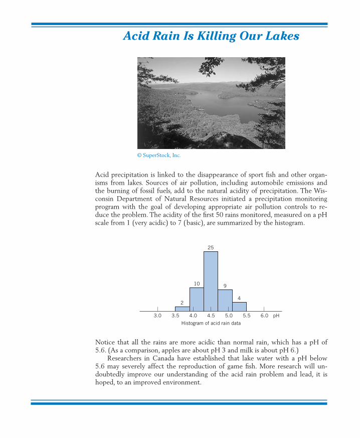
Acid precipitation is linked to the disappearance of sport fish and other organ-isms from lakes. Sources of air pollution, including automobile emissions andthe burning of fossil fuels, add to the natural acidity of precipitation. The Wis-consin Department of Natural Resources initiated a precipitation monitoringprogram with the goal of developing appropriate air pollution controls to re-duce the problem. The acidity of the first 50 rains monitored, measured on a pHscale from 1 (very acidic) to 7 (basic), are summarized by the histogram.
Notice that all the rains are more acidic than normal rain, which has a pH of5.6. (As a comparison, apples are about pH 3 and milk is about pH 6.)
Researchers in Canada have established that lake water with a pH below5.6 may severely affect the reproduction of game fish. More research will un-doubtedly improve our understanding of the acid rain problem and lead, it ishoped, to an improved environment.
© SuperStock, Inc.
c02a.qxd 10/15/09 12:02 PM Page 22

1. INTRODUCTION
In Chapter 1, we cited several examples of situations where the collection ofdata by appropriate processes of experimentation or observation is essential toacquire new knowledge. A data set may range in complexity from a few entriesto hundreds or even thousands of them. Each entry corresponds to the observa-tion of a specified characteristic of a sampling unit. For example, a nutritionistmay provide an experimental diet to 30 undernourished children and recordtheir weight gains after two months. Here, children are the sampling units, andthe data set would consist of 30 measurements of weight gains. Once the dataare collected, a primary step is to organize the information and extract a de-scriptive summary that highlights its salient features. In this chapter, we learnhow to organize and describe a set of data by means of tables, graphs, and calcu-lation of some numerical summary measures.
2. MAIN TYPES OF DATA
In discussing the methods for providing summary descriptions of data, it helpsto distinguish between the two basic types:
1. Qualitative or categorical data
2. Numerical or measurement data
When the characteristic under study concerns a qualitative trait that is onlyclassified in categories and not numerically measured, the resulting data arecalled categorical data. Hair color (blond, brown, red, black), employment sta-tus (employed, unemployed), and blood type (O, A, B, AB) are but some exam-ples. If, on the other hand, the characteristic is measured on a numerical scale,the resulting data consist of a set of numbers and are called measurement data.We will use the term numerical-valued variable or just variable to refer to acharacteristic that is measured on a numerical scale. The word “variable” signifiesthat the measurements vary over different sampling units. In this terminology,observations of a numerical-valued variable yield measurement data. A few ex-amples of numerical-valued variables are the shoe size of an adult male, dailynumber of traffic fatalities in a state, intensity of an earthquake, height of a 1-year-old pine seedling, the time in line at an automated teller, and the numberof offspring in an animal litter.
Although in all these examples the stated characteristic can be numeri-cally measured, a close scrutiny reveals two distinct types of underlying scaleof measurement. Shoe sizes are numbers such as 6, 6 7, 7 . . . , whichproceed in steps of The count of traffic fatalities can only be an integer andso is the number of offspring in an animal litter. These are examples of dis-crete variables. The name discrete draws from the fact that the scale is madeup of distinct numbers with gaps in between. On the other hand, some vari-ables such as height, weight, and survival time can ideally take any value in an
12 .
12 ,1
2 ,
2. MAIN TYPES OF DATA 23
c02a.qxd 10/15/09 12:02 PM Page 23

interval. Since the measurement scale does not have gaps, such variables arecalled continuous.
We must admit that a truly continuous scale of measurement is an idealiza-tion. Measurements actually recorded in a data set are always rounded either forthe sake of simplicity or because the measuring device has a limited accuracy.Still, even though weights may be recorded in the nearest pounds or timerecorded in the whole hours, their actual values occur on a continuous scale sothe data are referred to as continuous. Counts are inherently discrete andtreated as such, provided that they take relatively few distinct values (e.g., thenumber of children in a family or the number of traffic violations of a driver).But when a count spans a wide range of values, it is often treated as a continu-ous variable. For example, the count of white blood cells, number of insects in acolony, and number of shares of stock traded per day are strictly discrete, but forpractical purposes, they are viewed as continuous.
A summary description of categorical data is discussed in Section 3.1. Theremainder of this chapter is devoted to a descriptive study of measurementdata, both discrete and continuous. As in the case of summarization and com-mentary on a long, wordy document, it is difficult to prescribe concrete steps forsummary descriptions that work well for all types of measurement data. How-ever, a few important aspects that deserve special attention are outlined here toprovide general guidelines for this process.
3. DESCRIBING DATA BY TABLES AND GRAPHS
3.1 CATEGORICAL DATA
When a qualitative trait is observed for a sample of units, each observation isrecorded as a member of one of several categories. Such data are readily orga-nized in the form of a frequency table that shows the counts (frequencies) ofthe individual categories. Our understanding of the data is further enhanced by
24 CHAPTER 2/ORGANIZATION AND DESCRIPTION OF DATA
Describing a Data Set of Measurements
1. Summarization and description of the overall pattern.(a) Presentation of tables and graphs.(b) Noting important features of the graphed data including symme-
try or departures from it.(c) Scanning the graphed data to detect any observations that seem
to stick far out from the major mass of the data—the outliers.
2. Computation of numerical measures.(a) A typical or representative value that indicates the center of the
data.(b) The amount of spread or variation present in the data.
c02a.qxd 10/15/09 12:02 PM Page 24

calculation of the proportion (also called relative frequency) of observations ineach category.
Example 1 Calculating Relative Frequencies to Summarize an Opinion PollA campus press polled a sample of 280 undergraduate students in order tostudy student attitude toward a proposed change in the dormitory regula-tions. Each student was to respond as support, oppose, or neutral in regard tothe issue. The numbers were 152 support, 77 neutral, and 51 opposed. Tabu-late the results and calculate the relative frequencies for the three responsecategories.
SOLUTION Table 1 records the frequencies in the second column, and the relative fre-quencies are calculated in the third column. The relative frequencies showthat about 54% of the polled students supported the change, 18% opposed,and 28% were neutral.
Remark: The relative frequencies provide the most relevant informationas to the pattern of the data. One should also state the sample size, whichserves as an indicator of the credibility of the relative frequencies. (More onthis in Chapter 8.)
Categorical data are often presented graphically as a pie chart in which thesegments of a circle exhibit the relative frequencies of the categories. To obtainthe angle for any category, we multiply the relative frequency by 360 degrees,
3. DESCRIBING DATA BY TABLES AND GRAPHS 25
Relative frequencyof a category �
Frequency in the categoryTotal number of observations
TABLE 1 Summary Resultsof an Opinion Poll
RelativeResponses Frequency Frequency
Support 152
Neutral 77
Oppose 51
Total 280 1.000
51280
� .182
77280
� .275
152280
� .543
c02a.qxd 10/15/09 12:02 PM Page 25

which corresponds to the complete circle. Although laying out the angles byhand can be tedious, many software packages generate the chart with a singlecommand. Figure 1 presents a pie chart for the data in Example 1.
When questions arise that need answering but the decision makers lack pre-cise knowledge of the state of nature or the full ramifications of their decisions,the best procedure is often to collect more data. In the context of quality im-provement, if a problem is recognized, the first step is to collect data on themagnitude and possible causes. This information is most effectively communi-cated through graphical presentations.
A Pareto diagram is a powerful graphical technique for displaying eventsaccording to their frequency. According to Pareto’s empirical law, any collectionof events consists of only a few that are major in that they are the ones that oc-cur most of the time.
Figure 2 gives a Pareto diagram for the type of defects found in a day’s pro-duction of facial tissues. The cumulative frequency is 22 for the first cause and
26 CHAPTER 2/ORGANIZATION AND DESCRIPTION OF DATA
Oppose18%
Neutral28%
Support54%
20
15
10
Freq
uenc
y
Tears Holes Folds Other
5
0
Figure 1 Pie chart of studentopinion on change in dormitoryregulations.
Figure 2 Pareto diagram of facial tissue defects.
c02a.qxd 10/15/09 12:02 PM Page 26

22 � 15 � 37 for the first and second causes combined. This illustratesPareto’s rule, with two of the causes being responsible for 37 out of 50, or 74%,of the defects.
Example 2 A Pareto Diagram Clarifies Circumstances Needing ImprovementGraduate students in a counseling course were asked to choose one of theirpersonal habits that needed improvement. In order to reduce the effect ofthis habit, they were asked to first gather data on the frequency of the occur-rence and the circumstances. One student collected the following frequencydata on fingernail biting over a two-week period.
Make a Pareto diagram showing the relationship between nail biting andtype of activity.
SOLUTION The cumulative frequencies are 58, 58 � 21 � 79, and so on, out of 115.The Pareto diagram is shown in Figure 3, where watching TV accounts for50.4% of the instances.
The next step for this person would be to try and find a substitute fornail biting while watching television.
3. DESCRIBING DATA BY TABLES AND GRAPHS 27
60
Freq
uenc
y
50
40
30
20
10
0TV Paper Phone Driving Shopping Other
Figure 3 Pareto diagram for nail biting example.
Frequency Activity
58 Watching television21 Reading newspaper14 Talking on phone7 Driving a car3 Grocery shopping
12 Other
c02a.qxd 10/15/09 12:02 PM Page 27

3.2 DISCRETE DATA
We next consider summary descriptions of measurement data and begin our dis-cussion with discrete measurement scales. As explained in Section 2, a data setis identified as discrete when the underlying scale is discrete and the distinct val-ues observed are not too numerous.
Similar to our description of categorical data, the information in a discretedata set can be summarized in a frequency table, or frequency distributionthat includes a calculation of the relative frequencies. In place of the qualitativecategories, we now list the distinct numerical measurements that appear in thedata set and then count their frequencies.
Example 3 Creating a Frequency DistributionRetail stores experience their heaviest returns on December 26 and December27 each year. Most are gifts that, for some reason, did not please the recipient.The number of items returned, by a sample of 30 persons at a large discount de-partment store, are observed and the data of Table 2 are obtained. Determinethe frequency distribution.
SOLUTION The frequency distribution of these data is presented in Table 3. The valuesare paired with the frequency and the calculated relative frequency.
28 CHAPTER 2/ORGANIZATION AND DESCRIPTION OF DATA
TABLE 2 Number of items returned
1 4 3 2 3 4 5 1 2 12 5 1 4 2 1 3 2 4 12 3 2 3 2 1 4 3 2 5
TABLE 3 Frequency Distribution forNumber (x) of Items Returned
Value x Frequency Relative Frequency
1 7 .2332 9 .3003 6 .2004 5 .1675 3 .100
Total 30 1.000
c02a.qxd 10/15/09 12:02 PM Page 28

The frequency distribution of a discrete variable can be presented pictori-ally by drawing either lines or rectangles to represent the relative frequencies.First, the distinct values of the variable are located on the horizontal axis. For aline diagram, we draw a vertical line at each value and make the height of theline equal to the relative frequency. A histogram employs vertical rectanglesinstead of lines. These rectangles are centered at the values and their areas rep-resent relative frequencies. Typically, the values proceed in equal steps so therectangles are all of the same width and their heights are proportional to the rel-ative frequencies as well as frequencies. Figure 4(a) shows the line diagram and4(b) the histogram of the frequency distribution of Table 3.
3.3 DATA ON A CONTINUOUS VARIABLE
We now consider tabular and graphical presentations of data sets that containnumerical measurements on a virtually continuous scale. Of course, therecorded measurements are always rounded. In contrast with the discrete case, adata set of measurements on a continuous variable may contain many distinctvalues. Then, a table or plot of all distinct values and their frequencies will notprovide a condensed or informative summary of the data.
The two main graphical methods used to display a data set of measure-ments are the dot diagram and the histogram. Dot diagrams are employedwhen there are relatively few observations (say, less than 20 or 25); histogramsare used with a larger number of observations.
Dot Diagram
When the data consist of a small set of numbers, they can be graphically repre-sented by drawing a line with a scale covering the range of values of the mea-surements. Individual measurements are plotted above this line as prominentdots. The resulting diagram is called a dot diagram.
3. DESCRIBING DATA BY TABLES AND GRAPHS 29
Figure 4 Graphic display of the frequency distribution of data in Table 3.
0 1 2 3 4(a) Line diagram
5 x 0 1 2 3 4(b) Histogram
5 x
Rel
ativ
e fr
eque
ncy
0.3
0.2
0.1
0.3
0.2
0.1Rel
ativ
e fr
eque
ncy
c02a.qxd 10/15/09 12:02 PM Page 29

Example 4 A Dot Diagram Reveals an Unusual ObservationThe number of days the first six heart transplant patients at Stanford sur-vived after their operations were 15, 3, 46, 623, 126, 64. Make a dot diagram.
SOLUTION These survival times extended from 3 to 623 days. Drawing a line segmentfrom 0 to 700, we can plot the data as shown in Figure 5. This dot diagramshows a cluster of small survival times and a single, rather large value.
Frequency Distribution on Intervals
When the data consist of a large number of measurements, a dot diagram maybe quite tedious to construct. More seriously, overcrowding of the dots willcause them to smear and mar the clarity of the diagram. In such cases, it is con-venient to condense the data by grouping the observations according to intervalsand recording the frequencies of the intervals. Unlike a discrete frequency distri-bution, where grouping naturally takes place on points, here we use intervals ofvalues. The main steps in this process are outlined as follows.
The choice of the number and position of the class intervals is primarily amatter of judgment guided by the following considerations. The number of
30 CHAPTER 2/ORGANIZATION AND DESCRIPTION OF DATA
0 100 200 300Survival time (days)
400 500 600 700
Figure 5 Dot diagram for the heart transplant data.
Constructing a Frequency Distribution for a Continuous Variable
1. Find the minimum and the maximum values in the data set.
2. Choose intervals or cells of equal length that cover the range betweenthe minimum and the maximum without overlapping. These arecalled class intervals, and their endpoints class boundaries.
3. Count the number of observations in the data that belong to eachclass interval. The count in each class is the class frequency or cell fre-quency.
4. Calculate the relative frequency of each class by dividing the class fre-quency by the total number of observations in the data:
Relative frequency �Class frequency
Total number of observations
c02a.qxd 10/15/09 12:02 PM Page 30

Paying Attention
First-grade teachers allot a portion of each day to mathematics. An ed-ucator, concerned about how students utilize this time, selected 24 stu-dents and observed them for a total of 20 minutes spread over severaldays. The number of minutes, out of 20, that the student was not on taskwas recorded (courtesy of T. Romberg). These lack-of-attention times aregraphically portrayed in the dot diagram in Figure 6. The student with 13out of 20 minutes off-task stands out enough to merit further considera-tion. Is this a student who finds the subject too difficult or might it be avery bright child who is bored?
classes usually ranges from 5 to 15, depending on the number of observations inthe data. Grouping the observations sacrifices information concerning how theobservations are distributed within each cell. With too few cells, the loss of in-formation is serious. On the other hand, if one chooses too many cells and the
3. DESCRIBING DATA BY TABLES AND GRAPHS 31
Figure 6 Time not concentrating on the mathe-matics assignment (out of 20 minutes).
0 1
Paying attention in class. Observations on 24 rst grade students.
2 3 4 5 6 7Minutes
8 9 10 11 12 13
Paying attention in class. Observations on 24 first-grade students.© Britt Erlanson/The Image Bank/Getty Images
c02a.qxd 10/15/09 12:02 PM Page 31

data set is relatively small, the frequencies from one cell to the next wouldjump up and down in a chaotic manner and no overall pattern would emerge.As an initial step, frequencies may be determined with a large number of inter-vals that can later be combined as desired in order to obtain a smooth pattern ofthe distribution.
Computers conveniently order data from smallest to largest so that the ob-servations in any cell can easily be counted. The construction of a frequency dis-tribution is illustrated in Example 5.
Example 5 Creating a Frequency Distribution for Hours of SleepStudents require different amounts of sleep. A sample of 59 students at a largemidwest university reported the following hours of sleep the previous night.
Construct a frequency distribution of the sleep data.
SOLUTION To construct a frequency distribution, we first notice that the minimumhours of sleep is 4.5 and the maximum is 10.0. We choose class intervals oflength 1.2 hours as a matter of convenience.
The selection of class boundaries is a bit of fussy work. Because the datahave one decimal place, we could add a second decimal to avoid the possibil-ity of any observation falling exactly on the boundary. For example, we couldend the first class interval at 5.45. Alternatively, and more neatly, we couldwrite 4.3–5.5 and make the endpoint convention that the left-hand endpoint is included but not the right.
The first interval contains 5 observations so its frequency is 5 and its rel-ative frequency is Table 5 gives the frequency distribution. Therelative frequencies add to 1, as they should (up to rounding error) for anyfrequency distribution. We see, for instance, that just about one-third of thestudents .271 + .051 = .322 got 7.9 hours or more of sleep.
Remark: The rule requiring equal class intervals is inconvenient whenthe data are spread over a wide range but are highly concentrated in asmall part of the range with relatively few numbers elsewhere. Usingsmaller intervals where the data are highly concentrated and larger inter-vals where the data are sparse helps to reduce the loss of information dueto grouping.
559 � .085.
32 CHAPTER 2/ORGANIZATION AND DESCRIPTION OF DATA
TABLE 4 Hours of Sleep for Fifty-nine Students
4.5 4.7 5.0 5.0 5.3 5.5 5.5 5.7 5.7 5.76.0 6.0 6.0 6.0 6.3 6.3 6.3 6.5 6.5 6.56.7 6.7 6.7 6.7 7.0 7.0 7.0 7.0 7.3 7.37.3 7.3 7.5 7.5 7.5 7.5 7.7 7.7 7.7 7.78.0 8.0 8.0 8.0 8.3 8.3 8.3 8.5 8.5 8.58.5 8.7 8.7 9.0 9.0 9.0 9.3 9.3 10.0
c02a.qxd 10/15/09 12:02 PM Page 32

In every application involving an endpoint convention, it is important that youclearly state which endpoint is included and which is excluded. This informationshould be presented in the title or in a footnote of any frequency distribution.
Histogram
A frequency distribution can be graphically presented as a histogram. To draw ahistogram, we first mark the class intervals on the horizontal axis. On each interval,we then draw a vertical rectangle whose area represents the relative frequency—that is, the proportion of the observations occurring in that class interval.
To create rectangles whose area is equal to relative frequency, use the rule
The total area of all rectangles equals 1, the sum of the relative frequencies.
The histogram for Table 5 is shown in Figure 7. For example, the rectangledrawn on the class interval 4.3–5.5 has area � .071 � 1.2 � .085, which isthe relative frequency of this class. Actually, we determined the height .071 as
The units on the vertical axis can be viewed as relative frequencies per unitof the horizontal scale. For instance, .071 is the relative frequency per hour forthe interval 4.3–5.5.
Height �Relative frequencyWidth of interval
�.0851.2
� .071
Height �Relative frequencyWidth of interval
3. DESCRIBING DATA BY TABLES AND GRAPHS 33
The total area of a histogram is 1.
TABLE 5 Frequency Distribution for Hours of Sleep Data (leftendpoints included but right endpoints excluded)
Class Interval Frequency Relative Frequency
4.3–5.5 5
5.5–6.7 15
6.7–7.9 20
7.9–9.1 16
9.1–10.3 3
Total 59 1.000
359
� .051
1659
� .271
2059
� .339
1559
� .254
559
� .085
c02a.qxd 10/15/09 12:02 PM Page 33

Visually, we note that the rectangle having largest area, or most frequent classinterval, is 6.7–7.9. Also, proportion .085 � .254 � .339 of the students sleptless than 6.7 hours.
Remark: When all class intervals have equal widths, the heights of the rectan-gles are proportional to the relative frequencies that the areas represent. Theformal calculation of height, as area divided by the width, is then redundant. In-stead, one can mark the vertical scale according to the relative frequencies—that is, make the heights of the rectangles equal to the relative frequencies. Theresulting picture also makes the areas represent the relative frequencies if weread the vertical scale as if it is in units of the class interval. This leeway whenplotting the histogram is not permitted in the case of unequal class intervals.
Figure 8 shows one ingenious way of displaying two histograms for comparison.In spite of their complicated shapes, their back-to-back plot as a “tree” allows foreasy visual comparison. Females are the clear majority in the last age groups ofthe male and female age distributions.
Stem-and-Leaf Display
A stem-and-leaf display provides a more efficient variant of the histogram fordisplaying data, especially when the observations are two-digit numbers. Thisplot is obtained by sorting the observations into rows according to their leadingdigit. The stem-and-leaf display for the data of Table 6 is shown in Table 7. Tomake this display:
1. List the digits 0 through 9 in a column and draw a vertical line. Thesecorrespond to the leading digit.
2. For each observation, record its second digit to the right of this verticalline in the row where the first digit appears.
3. Finally, arrange the second digits in each row so they are in increasing order.
34 CHAPTER 2/ORGANIZATION AND DESCRIPTION OF DATA
0.3
0.2
Rel
ativ
e fr
eque
ncy
per
hour
0.1
0.4
4.3 5.5
.085
.254
.339
.271
.051
6.7
Hours sleep
7.9 9.1 10.3
Figure 7 Histogram of the sleep data of Tables 4 and 5.Sample size � 59.
c02a.qxd 10/15/09 12:02 PM Page 34

3. DESCRIBING DATA BY TABLES AND GRAPHS 35
0 100 100 and overAge
N = 148.7 million
N = 153.0 million
Mal
eFe
mal
e10 20 30 40 50 60 70 80 90
Figure 8 Population tree (histograms) of the male and female age distribu-tions in the United States in 2007. (Source: U.S. Bureau of the Census.)
TABLE 6 Examination Scores of 50 Students
75 98 42 75 84 87 65 59 6386 78 37 99 66 90 79 80 8968 57 95 55 79 88 76 60 7749 92 83 71 78 53 81 77 5893 85 70 62 80 74 69 90 6284 64 73 48 72
TABLE 7 Stem-and-Leaf Display for the Examination Scores
0123 74 2895 357896 0223456897 012345567788998 001344567899 0023589
c02a.qxd 10/15/09 12:02 PM Page 35

2.1 Cities must find better ways to dispose ofsolid waste. According to the EnvironmentalProtection Agency, the composition of the 254million tons of solid municipal waste createdin 2007 was
(a) Determine the percentage of other mate-rials in the solid waste. This category in-cludes glass, wood, rubber, and so on.
(b) Create a Pareto chart.
(c) What percentage of the total solid wasteis paper or paperboard? What percentageis from the top two categories? What per-centage is from the top five categories?
2.2 Recorded here are the blood types of 40 per-sons who have volunteered to donate blood ata plasma center. Summarize the data in a fre-quency table. Include calculations of the rela-tive frequencies.
In the stem-and-leaf display, the column of first digits to the left of the ver-tical line is viewed as the stem, and the second digits as the leaves. Viewed side-wise, it looks like a histogram with a cell width equal to 10. However, it is moreinformative than a histogram because the actual data points are retained. In fact,every observation can be recovered exactly from this stem-and-leaf display.
A stem-and-leaf display retains all the information in the leading digits ofthe data. When the leaf unit � .01, 3.5&0 2 3 7 8 presents the data 3.50, 3.52,3.53, 3.57, and 3.58. Leaves may also be two-digit at times. When the first leaf digit� .01, .4&07 13 82 90 presents the data 0.407, 0.413, 0.482, and 0.490.
Further variants of the stem-and-leaf display are described in Exercises 2.25and 2.26. This versatile display is one of the most applicable techniques of ex-ploratory data analysis.
When the sample size is small or moderate, no information is lost with thestem-and-leaf diagram because you can see every data point. The major disad-vantage is that, when the sample size is large, diagrams with hundreds of num-bers in a row cannot be constructed in a legible manner.
Exercises
36 CHAPTER 2/ORGANIZATION AND DESCRIPTION OF DATA
Paper and paperboard 32.7%Yard waste 12.8%Food waste 12.5%Plastics 12.1%Metals 8.2%Other materials
O O A B A O A A A OB O B O O A O O A AA A AB A B A A O O AO O A A A O A O O AB
2.3 A student at the University of Wisconsin surveyed40 students in her dorm concerning their partic-ipation in extracurricular activities during thepast week. The data on number of activities are
1 5 0 1 4 3 0 2 1 6 1 1 0 02 0 0 3 1 2 1 2 2 2 2 2 1 02 2 3 4 2 7 2 2 3 3 1 1
Present these data in a frequency table and in arelative frequency bar chart.
2.4 The number of automobile accidents reportedper month helps to identify intersections that re-quire improvement. Beginning January 2004 andending November 2008, the number of crashesper month reported at an intersection near a uni-versity campus in Madison,Wisconsin, are
1 3 3 3 2 2 3 1 2 4 1 41 3 1 1 1 0 1 2 2 5 5 25 5 4 3 3 6 1 2 3 2 4 34 4 3 5 3 3 3 5 1 5 5 34 2 2 0 0 1 4 1 0 2 0
c02a.qxd 10/15/09 12:02 PM Page 36

Present these data in a frequency table and in arelative frequency bar chart.
2.5 The following table shows how workers in onedepartment get to work.
(a) Calculate the relative frequency of eachmode of transportation.
(b) Construct a pie chart.
2.6 Of the $207 million raised by a major uni-versity’s fund drive, $117 million came fromindividuals and bequests, $24 million from in-dustry and business, and $66 million fromfoundations and associations. Present this in-formation in the form of a pie chart.
2.7 Data from one campus dorm on the number ofburglaries are collected each week of the se-mester. These data are to be grouped into theclasses 0–1, 2–3, 3–5, 6 or more. Both end-points included. Explain where a difficultymight arise.
2.8 Data from one campus dorm, on the numberof complaints about the dorm food are col-lected each week of the semester. These weeklycounts are to be grouped into the classes 0–1,2–3, 4–5, 7 or more. Both endpoints are in-cluded. Explain where a difficulty might arise.
2.9 A sample of persons will each be asked to givethe number of their close friends. The re-sponses are to be grouped into the followingclasses: 0, 1–3, 3–5, 6 or more. Left endpoint isincluded. Explain where difficulties might arise.
2.10 The weights of the players on the universityfootball team (to the nearest pound) are to begrouped into the following classes: 160–175,175–190, 190–205, 205–220, 220–235, 235or more. The left endpoint is included but notthe right endpoint. Explain where difficultiesmight arise.
2.11 On flights from San Francisco to Chicago, thenumber of empty seats are to be grouped intothe following classes: 0–4, 5–9, 10–14, 15–19,more than 19.
Is it possible to determine from this frequencydistribution the exact number of flights onwhich there were:
(a) Fewer than 10 empty seats?
(b) More than 14 empty seats?
(c) At least 5 empty seats?
(d) Exactly 9 empty seats?
(e) Between 5 and 15 empty seats inclusively?
2.12 A major West Coast power company sur-veyed 50 customers who were asked to re-spond to the statement, “People should relymainly on themselves to solve problemscaused by power outages” with one of the fol-lowing responses.
1. Definitely agree.
2. Somewhat agree.
3. Somewhat disagree.
4. Definitely disagree.
The responses are as follows:
4 2 1 3 3 2 4 2 1 1 2 2 2 2 1 3 41 4 4 1 3 2 4 1 4 3 3 1 1 1 2 1 14 4 4 4 4 1 2 2 2 4 4 4 1 3 4 2
Construct a frequency table.
2.13 A sample of 50 departing airline passengers atthe main check-in counter produced the fol-lowing number of bags checked through to fi-nal destinations.
0 1 2 2 1 2 1 2 3 0 1 01 1 0 1 3 0 1 2 1 1 1 21 2 2 1 2 0 0 2 2 1 1 11 1 1 1 2 0 1 3 0 1 2 11 3
(a) Make a relative frequency line diagram.
(b) Comment on the pattern.
(c) What proportion of passengers whocheck in at the main counter fail to checkany bags?
3. DESCRIBING DATA BY TABLES AND GRAPHS 37
Mode ofTransportation Frequency
Drive alone 25Car pool 3Ride bus 7Other 5
c02a.qxd 10/15/09 12:02 PM Page 37

2.14 A person with asthma took measurements byblowing into a peak-flow meter on seven con-secutive days.
429 425 471 422 432 444 454
Display the data in a dot diagram.
2.15 Before microwave ovens are sold, the manu-facturer must check to ensure that the radia-tion coming through the door is below a speci-fied safe limit. The amounts of radiationleakage (mW/cm2) with the door closed from25 ovens are as follows (courtesy of JohnCryer):
15 9 18 10 5 12 85 8 10 7 2 15 3 5 15 10 159 8 18 1 2 11
Display the data in a dot diagram.
2.16 A campus area merchant recorded the numberof bad checks received per month, for fivemonths
4 5 4 7 6
Display the data in a dot diagram.
2.17 The city of Madison regularly checks the water quality at swimming beaches locatedon area lakes. The concentration of fecal coliforms, in number of colony forming units (CFU) per 100 ml of water, was mea-sured on fifteen days during the summer atone beach.
180 1600 90 140 50 260 400 90380 110 10 60 20 340 80
(a) Make a dot diagram.
(b) Comment on the pattern and any unusualfeatures.
(c) The city closes any swimming beach if acount is over 1350. What proportion ofdays, among the fifteen, was this beachclosed?
38 CHAPTER 2/ORGANIZATION AND DESCRIPTION OF DATA
Number of Deaths Frequency
24 or less 225–49 2050–74 1875–99 7
100–149 6150–199 2200–249 1
250 or more 3
Total 59
(a) Calculate the relative frequency for theintervals [0, 25), [25, 50) and so onwhere the right-hand endpoint is ex-cluded. Take the last interval to be[250, 550).
(b) Plot the relative frequency histogram.(Hint: Since the intervals have unequalwidths, make the height of each rectangleequal to the relative frequency divided bythe width of the interval.)
(c) What proportion of the years had 49 orfewer deaths due to tornadoes?
(d) Comment on the shape of the distribution.
2.19 A zoologist collected wild lizards in theSouthwestern United States. Thirty lizardsfrom the genus Phrynosoma were placed ona treadmill and their speed measured. Therecorded speed (meters/second) is thefastest time to run a half meter. (Courtesy ofK. Bonine.)
1.28 1.36 1.24 2.47 1.94 2.52 2.67 1.291.56 2.66 2.17 1.57 2.10 2.54 1.63 2.112.57 1.72 0.76 1.02 1.78 0.50 1.49 1.571.04 1.92 1.55 1.78 1.70 1.20
2.18 Tornadoes kill many people every year in theUnited States. The yearly number of lives lostduring the 59 years 1950 through 2008 aresummarized in the following table.
c02a.qxd 10/15/09 12:02 PM Page 38

(a) Construct a frequency distribution usingthe class intervals 0.45–0.90, 0.90–1.35,and so on, with the endpoint conventionthat the left endpoint is included and theright endpoint is excluded. Calculate therelative frequencies.
(b) Make a histogram.
2.20 The United States Geological Survey main-tains data on large earthquakes including thoseof magnitude greater than 6.0 in California.Through 2008, the ordered magnitudes of the55 quakes are
6.1 6.1 6.1 6.1 6.1 6.2 6.2 6.2 6.2 6.3 6.36.3 6.4 6.4 6.4 6.4 6.4 6.4 6.4 6.5 6.5 6.56.5 6.5 6.6 6.6 6.6 6.7 6.7 6.7 6.8 6.8 6.86.8 6.8 6.9 6.9 7.0 7.0 7.0 7.1 7.1 7.1 7.27.2 7.2 7.2 7.3 7.3 7.3 7.3 7.4 7.8 7.8 7.9
Construct a histogram using equal-length in-tervals starting with (6.0, 6.3] where theright-hand endpoint is included but not theleft-hand endpoint.
2.21 Referring to Exercise 2.20, construct a densityhistogram using the intervals (6.0, 6.3], (6.3,6.6], (6.6, 6.9], (6.9, 7.2], and (7.2, 7.9].
2.22 The following data represent the scores of 40students on a college qualification test (cour-tesy of R. W. Johnson).
162 171 138 145 144 126 145 162 174 178167 98 161 152 182 136 165 137 133 143184 166 115 115 95 190 119 144 176 135194 147 160 158 178 162 131 106 157 154
Make a stem-and-leaf display.
2.23 A federal government study of the oil reservesin Elk Hills, CA, included a study of theamount of iron present in the oil.
3. DESCRIBING DATA BY TABLES AND GRAPHS 39
Make a stem-and-leaf display.
2.24 The following is a stem-and-leaf display withtwo-digit leaves. (The leading leaf digit � 10.0.)
12 46 68 933 19 44 71 82 974 05 26 43 905 04 686 13
List the corresponding measurements.
2.25 If there are too many leaves on some stems ina stem-and-leaf display, we might double thenumber of stems. The leaves 0–4 could hangon one stem and 5–9 on the repeated stem. Forthe observations
193 198 200 202 203 203 205 205 206 207207 208 212 213 214 217 219 220 222 226 237
we would get the double-stem display
19 319 820 023320 55677821 23421 7922 0222 62323 7
Amount of Iron (percent ash)
20 18 25 26 1714 20 14 18 1522 15 17 25 2212 52 27 24 4134 20 17 20 1920 16 20 15 3422 29 29 34 2713 6 24 47 3212 17 36 35 4136 32 46 30 51
c02a.qxd 10/15/09 12:02 PM Page 39

Construct a double-stem display with one-digit leaves for the data of Exercise 2.22.
2.26 If the double-stem display still has too fewstems, we may wish to construct a stem-and-leaf display with a separate stem to hold leaves0 and 1, 2 and 3, 4 and 5, 6 and 7, and a stemto hold 8 and 9. The resulting stem-and-leafdisplay is called a five-stem display. The fol-lowing is a five-digit stem-and-leaf display.(Leaf unit � 1.0)
1 82 0012 22332 4445552 6672 93 0
List the corresponding measurements.
2.27 The following table lists values of the Con-sumer Price Index for 24 selected areas bothfor 2007 and 2001. Construct a five-stem dis-play for the consumer price index in 2007.
40 CHAPTER 2/ORGANIZATION AND DESCRIPTION OF DATA
2007 2001
Anchorage 181 155Atlanta 198 176Boston 227 191Chicago 198 178Cincinnati 188 168Cleveland 186 173Dallas 195 170Denver 194 181Detroit 195 174Honolulu 219 178Houston 182 159Kansas City 186 172Los Angeles 210 177Miami 210 173Milwaukee 198 172Minneapolis 195 177New York 221 187Philadelphia 216 181Pittsburgh 194 173Portland 203 182St. Louis 192 167San Diego 218 191San Francisco 211 190Seattle 210 186
4. MEASURES OF CENTER
The graphic procedures described in Section 3 help us to visualize the pattern ofa data set of measurements. To obtain a more objective summary description anda comparison of data sets, we must go one step further and obtain numerical val-ues for the location or center of the data and the amount of variability present.Because data are normally obtained by sampling from a large population, our dis-cussion of numerical measures is restricted to data arising in this context. More-over, when the population is finite and completely sampled, the same arithmeticoperations can be carried out to obtain numerical measures for the population.
To effectively present the ideas and associated calculations, it is convenientto represent a data set by symbols to prevent the discussion from becoming an-chored to a specific set of numbers. A data set consists of a number of measure-ments which are symbolically represented by , , . . . , . The last sub-script n denotes the number of measurements in the data, and , , . . .represent the first observation, the second observation, and so on. For instance, adata set consisting of the five measurements 2.1, 3.2, 4.1, 5.6, and 3.7 is repre-sented in symbols by , , , , , where � 2.1, � 3.2, � 4.1,
� 5.6, and � 3.7.x 5x 4
x 3x 2x1x 5x 4x 3x 2x1
x 2x1
x nx 2x1
c02a.qxd 10/15/09 12:02 PM Page 40

The most important aspect of studying the distribution of a sample of mea-surements is locating the position of a central value about which the measure-ments are distributed. The two most commonly used indicators of center are themean and the median.
The mean, or average, of a set of measurements is the sum of the measure-ments divided by their number. For instance, the mean of the five measurements2.1, 3.2, 4.1, 5.6, and 3.7 is
To state this idea in general terms, we use symbols. If a sample consists of nmeasurements , . . . , , the mean of the sample is
The notation will be used to represent a sample mean. To further simplify the writing of a sum, the Greek capital letter � (sigma) is used as a statistical short-hand. With this symbol:
For example, represents the sum
Remark: When the number of terms being summed is understood from
the context, we often simplify to � , instead of . Some further oper-
ations with the � notation are discussed in Appendix A1.
We are now ready to formally define the sample mean.
xi�n
i � 1xi
x1 � x2 � x3 � x4 � x5 .xi�5
i � 1
x
x 1 � x 2 � � � � � x n
n�
sum of the n measurementsn
xnx2x1,
2.1 � 3.2 � 4.1 � 5.6 � 3.75
�18.7
5� 3.74
4. MEASURES OF CENTER 41
The sum � � . . . � is denoted as .
Read this as “the sum of all with i ranging from 1 to n.”xi
xi�n
i � 1xnx2x1
The sample mean of a set of n measurements . . . , is the sumof these measurements divided by n. The sample mean is denoted by
x �
�n
i � 1 xi
n or � xi
n
x.xnx2,x1,
c02a.qxd 10/15/09 12:02 PM Page 41

According to the concept of “average,” the mean represents a center of adata set. If we picture the dot diagram of a data set as a thin weightless horizon-tal bar on which balls of equal size and weight are placed at the positions of thedata points, then the mean represents the point on which the bar will balance.The computation of the sample mean and its physical interpretation are illus-trated in Example 6.
Example 6 Calculating and Interpreting the Sample MeanThe birth weights in pounds of five babies born in a hospital on a certain day are9.2, 6.4, 10.5, 8.1, and 7.8. Obtain the sample mean and create a dot diagram.
SOLUTION The mean birth weight for these data is
The dot diagram of the data appears in Figure 9, where the sample mean(marked by �) is the balancing point or center of the picture.
Another measure of center is the middle value.
Roughly speaking, the median is the value that divides the data into two equalhalves. In other words, 50% of the data lie below the median and 50% above it.If n is an odd number, there is a unique middle value and it is the median. If n isan even number, there are two middle values and the median is defined as theiraverage. For instance, the ordered data 3, 5, 7, 8 have two middle values 5 and 7,so the median � (5 � 7)/2 � 6.
Example 7 Calculating the Sample MedianFind the median of the birth-weight data given in Example 6.
x �9.2 � 6.4 � 10.5 � 8.1 � 7.8
5�
42.05
� 8.4 pounds
x
42 CHAPTER 2/ORGANIZATION AND DESCRIPTION OF DATA
6 7 8 9 Poundsx
10 11
Figure 9 Dot diagram and the sample mean for the birth-weight data.
The sample median of a set of n measurements , . . . , is the mid-dle value when the measurements are arranged from smallest to largest.
xnx1
c02a.qxd 10/15/09 12:02 PM Page 42

SOLUTION The measurements, ordered from smallest to largest, are
6.4 7.8 9.2 10.5
The middle value is 8.1, and the median is therefore 8.1 pounds.
Example 8 Choosing between the Mean and MedianCalculate the median of the survival times given in Example 4. Also calculatethe mean and compare.
SOLUTION To find the median, first we order the data. The ordered values are
3 15 46 64 126 623
There are two middle values, so
The sample mean is
Note that one large survival time greatly inflates the mean. Only 1 out of the6 patients survived longer than days. Here the median of 55 daysappears to be a better indicator of the center than the mean.
Example 8 demonstrates that the median is not affected by a few very smallor very large observations, whereas the presence of such extremes can have aconsiderable effect on the mean. For extremely asymmetrical distributions, themedian is likely to be a more sensible measure of center than the mean. That iswhy government reports on income distribution quote the median income as asummary, rather than the mean. A relatively small number of very highly paidpersons can have a great effect on the mean salary.
If the number of observations is quite large (greater than, say, 25 or 30), it issometimes useful to extend the notion of the median and divide the ordereddata set into quarters. Just as the point for division into halves is called the me-dian, the points for division into quarters are called quartiles. The points of divi-sion into more general fractions are called percentiles.
The sample 100 p-th percentile is a value such that after the data areordered from smallest to largest, at least 100 p % of the observa-tions are at or below this value and at least 100 ( 1 � p ) % are ator above this value.
If we take the above conceptual description of the sample 100(.5) �50th percentile specifies that at least half the observations are equal or smaller
p � .5,
x � 146.2
x �3 � 15 � 46 � 64 � 126 � 623
6�
8776
� 146.2 days
Median �46 � 64
2� 55 days
8.1
4. MEASURES OF CENTER 43
c02a.qxd 10/15/09 12:02 PM Page 43

and at least half are equal or larger. If we take the sample 100(.25) �25th percentile has proportion one-fourth of the observations that are the sameor smaller and proportion three-fourths that are the same or larger.
We adopt the convention of taking an observed value for the sample per-centile except when two adjacent values satisfy the definition, in which casetheir average is taken as the percentile. This coincides with the way the medianis defined when the sample size is even. When all values in an interval satisfy thedefinition of a percentile, the particular convention used to locate a point in theinterval does not appreciably alter the results in large data sets, except perhapsfor the determination of extreme percentiles (those before the 5th or after the95th percentile).
The following operating rule will simplify the calculation of the sample per-centile.
The quartiles are simply the 25th, 50th, and 75th percentiles.
Example 9 Calculating Quartiles to Summarize Length of Phone CallsAn administrator wanted to study the utilization of long-distance telephoneservice by a department. One variable of interest is the length, in minutes, oflong-distance calls made during one month. There were 38 calls that resultedin a connection. The lengths of calls, already ordered from smallest to largest,are presented in Table 8. Locate the quartiles and also determine the 90thpercentile.
p � .25,
44 CHAPTER 2/ORGANIZATION AND DESCRIPTION OF DATA
Calculating the Sample 100p-th Percentile
1. Order the data from smallest to largest.
2. Determine the product (sample size) � ( proportion) � np.
If np is not an integer, round it up to the next integer and find the corre-sponding ordered value.
If np is an integer, say k, calculate the average of the kth and (k � 1)stordered values.
Sample Quartiles
Lower (first) quartile � 25th percentileSecond quartile (or median) � 50th percentileUpper (third) quartile � 75th percentileQ3
Q2
Q1
c02a.qxd 10/15/09 12:02 PM Page 44

SOLUTION To determine the first quartile, we take p � .25 and calculate the product38 � .25 � 9.5. Because 9.5 is not an integer, we take the next largest inte-ger, 10. In Table 8, we see that the 10th ordered observation is 4.4 so the firstquartile is � 4.4 minutes.
We confirm that this observation has 10 values at or below it and 29 val-ues at or above so that it does satisfy the conceptual definition of the firstquartile.
For the median, we take p � .5 and calculate 38 � .5 � 19. Becausethis is an integer, we average the 19th and 20th smallest observations to ob-tain the median, (9.3 � 9.5)/ 2 � 9.4 minutes.
Next, to determine the third quartile, we take p � .75 and calculate 38 � .75 � 28.5. The next largest integer is 29, so the 29th ordered obser-vation is the third quartile � 17.5 minutes. More simply, we couldmimic the calculation of the first quartile but now count down 10 observa-tions starting with the largest value.
For the 90th percentile, we determine 38 � .90 � 34.2, which we in-crease to 35. The 90th percentile is 31.7 minutes. Only 10% of calls last 31.7minutes or longer.
Exercises
Q3
Q1
4. MEASURES OF CENTER 45
2.28 Calculate the mean and median for each of thefollowing data sets.
(a) 3 7 4 11 5
(b) 3 1 7 3 1
2.29 Calculate the mean and median for each of thefollowing data sets.
(a) 2 5 1 4 3
(b) 26 30 38 32 26 31
(c) �1 2 0 1 4 �1 2
2.30 The height that bread rises may be one indica-tor of how light it will be. As a first step, before
modifying her existing recipe, a student cookmeasured the raise height (cm) on eight occa-sions:
6.3 6.9 5.7 5.4 5.6 5.5 6.6 6.5
Find the mean and median of the raised heights.
2.31 With reference to the water quality in Exercise2.17:
(a) Find the sample mean.
(b) Does the sample mean or the mediangive a better indication of the water qual-ity of a “typical” day? Why?
Table 8 The Lengths of Long-Distance Phone Calls in Minutes
1.6 1.7 1.8 1.8 1.9 2.1 2.5 3.0 3.0 4.44.5 4.5 5.9 7.1 7.4 7.5 7.7 8.6 9.3 9.5
12.7 15.3 15.5 15.9 15.9 16.1 16.5 17.3 17.5 19.019.4 22.5 23.5 24.0 31.7 32.8 43.5 53.3
c02a.qxd 10/15/09 12:02 PM Page 45

2.32 The monthly income in dollars for seven salespersons at a car dealership are
2450 2275 2425 4700 2650 2350 2475
(a) Calculate the mean and median salary.
(b) Which of the two is preferable as a mea-sure of center and why?
2.33 Records show that in Las Vegas, NV, the nor-mal daily maximum temperature (°F) for eachmonth starting in January is
56 62 68 77 87 99 105 102 95 82 66 57
Verify that the mean of these figures is 79.67.Comment on the claim that the daily maxi-mum temperature in Las Vegas averages apleasant 79.67.
2.34 A major wine producer reported sales (in hun-dreds of cases) for two-week periods duringone summer:
85 82 77 83 80 77 94
Obtain the sample mean and median.
2.35 With reference to the radiation leakage datagiven in Exercise 2.15:
(a) Calculate the sample mean.
(b) Which gives a better indication of theamount of radiation leakage, the samplemean or the median?
2.36 Recent crime reports on the number of aggra-vated assaults at each of the 27 largest univer-sities reporting for the year are summarized inthe computer output
Descriptive Statistics: AggAslt
Variable N Mean Median StDevAggAslt 27 10.30 10.00 7.61
Locate two measures of center tendency, or lo-cation, and interpret the values.
2.37 The weights (oz) of nineteen babies born inMadison, Wisconsin, are summarized in thecomputer output
Descriptive Statistics: Weight
Variable N Mean Median StDevWeight 19 118.05 117.00 15.47
46 CHAPTER 2/ORGANIZATION AND DESCRIPTION OF DATA
Locate two measures of center tendency, or lo-cation, and interpret the values.
2.38 With reference to the extracurricular activitiesdata in Exercise 2.3, obtain the
(a) sample mean.
(b) sample median.
(c) Comment on the effect of a large obser-vation.
2.39 With reference to the number of returns inExample 3, obtain the sample (a) mean and(b) median.
2.40 Old Faithful, the most famous geyser in Yellow-stone Park, had the following durations (mea-sured in seconds) in six consecutive eruptions:
240 248 113 268 117 253
(a) Find the sample median.
(b) Find the sample mean.
2.41 Loss of calcium is a serious problem for olderwomen. To investigate the amount of loss, a re-searcher measured the initial amount of bonemineral content in the radius bone of the dom-inant hand of elderly women and then theamount remaining after one year. The differ-ences, representing the loss of bone mineralcontent, are given in the following table (cour-tesy of E. Smith).
8 7 13 3 64 8 6 3 40 1 11 7 18 6 12 13 109 11 3 2 97 1 16 3 2
10 15 2 5 817 8 2 5 5
(a) Find the sample mean.
(b) Does the sample mean or the mediangive a better indication of the amount ofmineral loss?
2.42 Physical education researchers interested inthe development of the overarm throw mea-sured the horizontal velocity of a thrown ball
c02a.qxd 10/15/09 12:02 PM Page 46

at the time of release. The results for first-gradechildren (in feet/second) (courtesy of L.Halverson and M. Roberton) are
Males
54.2 39.6 52.3 48.4 35.9 30.4 25.2 45.4 48.9 48.945.8 44.0 52.5 48.3 59.9 51.7 38.6 39.1 49.9 38.3
Females
30.3 43.0 25.7 26.7 27.3 31.9 53.7 32.9 19.4 23.723.3 23.3 37.8 39.5 33.5 30.4 28.5
(a) Find the sample median for males.
(b) Find the sample median for females.
(c) Find the sample median for the combinedset of males and females.
2.43 On opening day one season, 10 major leaguebaseball games were played and they lasted thefollowing numbers of minutes.
167 211 187 176 170 158 198 218 145 232
Find the sample median.
2.44 If you were to use the data on the length ofmajor league baseball games in Exercise 2.43to estimate the total amount of digital mem-ory needed to film another 10 major leaguebaseball games, which is the more meaningfuldescription, the sample mean or the samplemedian? Explain.
2.45 The following measurements of the diame-ters (in feet) of Indian mounds in southernWisconsin were gathered by examining reports in the Wisconsin Archeologist (courtesy of J. Williams).
22 24 24 30 22 20 28 30 24 34 36 15 37
(a) Create a dot diagram.
(b) Calculate the mean and median and thenmark these on the dot diagram.
(c) Calculate the quartiles.
2.46 With reference to Exercise 2.3, calculate thequartiles.
4. MEASURES OF CENTER 47
2.47 Refer to the data of college qualification testscores given in Exercise 2.22.
(a) Find the median.
(b) Find and .
2.48 A large mail-order firm employs numerouspersons to take phone orders. Computers onwhich orders are entered also automaticallycollect data on phone activity. One variableuseful for planning staffing levels is the num-ber of calls per shift handled by each em-ployee. From the data collected on 25 work-ers, calls per shift were (courtesy of Land’sEnd)
118 118 57 92 127 109 96 68 7369 106 91 93 94 102 105 100 10480 50 96 82 72 108 73
Calculate the sample mean.
2.49 With reference to Exercise 2.48, calculate thequartiles.
2.50 The speedy lizard data, from Exercise 2.19,are
1.28 1.36 1.24 2.47 1.94 2.52 2.67 1.291.56 2.66 2.17 1.57 2.10 2.54 1.63 2.112.57 1.72 0.76 1.02 1.78 0.50 1.49 1.571.04 1.92 1.55 1.78 1.70 1.20
(a) Find the sample median, first quartile, andthird quartile.
(b) Find the sample 90th percentile.
2.51 With reference to the water quality data in Ex-ercise 2.17:
(a) Find the sample median, first quartile, andthird quartile.
(b) Find the sample 90th percentile.
2.52 Some properties of the mean and median.
1. If a fixed number c is added to all mea-surements in a data set, then the mean ofthe new measurements is
c � (the original mean).
2. If all measurements in a data set are multi-plied by a fixed number d, then the meanof the new measurements is
d � (the original mean).
Q3Q1
c02a.qxd 10/15/09 12:02 PM Page 47

5. MEASURES OF VARIATION
Besides locating the center of the data, any descriptive study of data must nu-merically measure the extent of variation around the center. Two data sets mayexhibit similar positions of center but may be remarkably different with respectto variability. For example, the dots in Figure 10b are more scattered than thosein Figure 10a.
(a) Verify these properties for the data set
4 8 8 7 9 6
taking in property (1) andin (2).
(b) The same properties also hold for the me-dian. Verify these for the data set and thenumbers c and d given in part (a).
2.53 On a day, the noon temperature measurements(in °F) reported by five weather stations in astate were
74 80 76 76 73
(a) Find the mean and median temperaturein °F.
(b) The Celsius (°C) scale is related to the Farenheit (°F) scale by C �What are the mean and median tempera-tures in °C? (Answer without convertingeach temperature measurement to °C.Use the properties stated in Exercise2.52.)
2.54 Given here are the mean and median salaries ofmachinists employed by two competing compa-nies A and B.
59 (F � 32).
d � 2c � 4
48 CHAPTER 2/ORGANIZATION AND DESCRIPTION OF DATA
Assume that the salaries are set in accordancewith job competence and the overall quality ofworkers is about the same in the two companies.
(a) Which company offers a better prospectto a machinist having superior ability?Explain your answer.
(b) Where can a medium-quality machinistexpect to earn more? Explain your answer.
2.55 Refer to the alligator data in Table D.11 of theData Bank. Using the data on testosterone for male alligators:
(a) Make separate dot plots for the LakeApopka and Lake Woodruff alligators.
(b) Calculate the sample means for eachgroup.
(c) Do the concentrations of testosterone ap-pear to differ between the two groups?What does this suggest the contaminationhas done to male alligators in the LakeApopka habitat?
2.56 Refer to the alligator data in Table D.11 of theData Bank. Using the data on testosterone from Lake Apopka:
(a) Make separate dot plots for the male andfemale alligators.
(b) Calculate the sample means for eachgroup.
(c) Do the concentrations of testosterone ap-pear to differ between the two groups?We would expect differences. What doesyour graph suggest the contamination hasdone to alligators in the Lake Apopkahabitat?
x4
x4
Company
A BMean salary $70,000 $65,500Median salary $56,000 $59,000
c02a.qxd 10/15/09 12:02 PM Page 48

Because the sample mean is a measure of center, the variation of the indi-vidual data points about this center is reflected in their deviation from the mean
For instance, the data set 3, 5, 7, 7, 8 has mean (3 � 5 � 7 � 7 �8)/5 � 30/5 � 6, so the deviations are calculated by subtracting 6 from eachobservation. See Table 9.
x �
� x � x Deviation � Observation � (Sample mean)
x
5. MEASURES OF VARIATION 49
0 5 10 x
0 5 10 x
(a)
(b)
Figure 10 Dot diagrams with similar center valuesbut different amounts of variation.
TABLE 9 Calculation of Deviations
Observation Deviationx
3 �35 �17 17 18 2
x � x
One might feel that the average of the deviations would provide a numeri-cal measure of spread. However, some deviations are positive and some nega-tive, and the total of the positive deviations exactly cancels the total of the nega-tive ones. In the foregoing example, we see that the positive deviations add to 4and the negative ones add to �4, so the total deviation is 0. With a little reflec-tion on the definition of the sample mean, the reader will realize that this wasnot just an accident. For any data set, the total deviation is 0 (for a formal proofof this fact, see Appendix A1).
� (Deviations) � � (xi � x) � 0
c02a.qxd 10/15/09 12:02 PM Page 49

To obtain a measure of spread, we must eliminate the signs of the devia-tions before averaging. One way of removing the interference of signs is tosquare the numbers. A measure of spread, called the sample variance, is con-structed by adding the squared deviations and dividing the total by the numberof observations minus one.
Example 10 Calculating Sample VarianceCalculate the sample variance of the data 3 5 7 7 8.
SOLUTION For this data set, To find the variance, we first calculate the mean,then the deviations and the squared deviations. See Table 10.
n � 5.
50 CHAPTER 2/ORGANIZATION AND DESCRIPTION OF DATA
Sample variance of n observations:
�
�n
i � 1 ( xi � x )2
n � 1
s 2 �sum of squared deviations
n � 1
TABLE 10 Calculation of Variance
Observation Deviation (Deviation)2
3 �3 95 �1 17 1 17 1 18 2 4
Total 30 0 16� x
Sample variance �16
5 � 1� 4s2
x �305
� 6
� ( x � x )2� ( x � x )
(x � x )2x � xx
c02a.qxd 10/15/09 12:02 PM Page 50

Example 11 Calculating the Sample Standard DeviationCalculate the standard deviation for the data of Example 10.
SOLUTION We already calculated the variance so the standard deviation is
To show that a larger spread of the data does indeed result in a larger numer-ical value of the standard deviation, we consider another data set in Example 12.
Example 12 Using Standard Deviations to Compare Variation in Two Data SetsCalculate the standard deviation for the data 1, 4, 5, 9, 11. Plot the dot dia-gram of this data set and also the data set of Example 10.
SOLUTION The standard deviation is calculated in Table 11. The dot diagrams, given inFigure 11, show that the data points of Example 10 have less spread thanthose of Example 12. This visual comparison is confirmed by a smaller valueof s for the first data set.
s � √4 � 2.s2 � 4
Remark: Although the sample variance is conceptualized as the averagesquared deviation, notice that the divisor is rather than n. The divi-sor, is called the degrees of freedom1 associated with s2.
Because the variance involves a sum of squares, its unit is the square of theunit in which the measurements are expressed. For example, if the data pertainto measurements of weight in pounds, the variance is expressed in (pounds)2. Toobtain a measure of variability in the same unit as the data, we take the positivesquare root of the variance, called the sample standard deviation. The standarddeviation rather than the variance serves as a basic measure of variability.
n � 1,n � 1
5. MEASURES OF VARIATION 51
1The deviations add to 0 so a specification of any deviations allows us to recover theone that is left out. For instance, the first four deviations in Example 10 add to �2, so to make thetotal 0, the last one must be �2, as it really is. In the definition of s2, the divisor representsthe number of deviations that can be viewed as free quantities.
n � 1
n � 1
Sample Standard Deviation
s � √Variance � � �n
i � 1 ( xi � x )2
n � 1
c02a.qxd 10/15/09 12:02 PM Page 51

An alternative formula for the sample variance is
It does not require the calculation of the individual deviations. In hand calcu-lation, the use of this alternative formula often reduces the arithmetic work,especially when turns out to be a number with many decimal places. Theequivalence of the two formulas is shown in Appendix A1.2.
Example 13 Calculating Sample Variance Using the Alternative FormulaIn a psychological experiment a stimulating signal of fixed intensity was usedon six experimental subjects. Their reaction times, recorded in seconds, were4, 2, 3, 3, 6, 3. Calculate the standard deviation for the data by using the al-ternative formula.
SOLUTION These calculations can be conveniently carried out in tabular form:
x
s2 �1
n � 1 �� xi
2 �� � xi �
2
n �
52 CHAPTER 2/ORGANIZATION AND DESCRIPTION OF DATA
0 2 4 6 8 10 12 14 16 18 20 x
(a)
0 2 4 6 8 10 12 14 16 18 20 x
(b)
Figure 11 Dot diagrams of two data sets.
TABLE 11 Calculation of s
x
1 �5 254 �2 45 �1 19 3 9
11 5 25
Total 30 0 64
s � √16 � 4
s 2 �644
� 16x � 6
( x � x )2( x � x )
c02a.qxd 10/15/09 12:02 PM Page 52

The reader may do the calculations with the first formula and verify thatthe same result is obtained.
In Example 12, we have seen that one data set with a visibly greater amount ofvariation yields a larger numerical value of s. The issue there surrounds a compari-son between different data sets. In the context of a single data set, can we relatethe numerical value of s to the physical closeness of the data points to the center
To this end, we view one standard deviation as a benchmark distance from themean For bell-shaped distributions, an empirical rule relates the standard devia-tion to the proportion of the data that lie in an interval around x.
x.x ?
5. MEASURES OF VARIATION 53
x x2
4 162 43 93 96 363 9
Total 21 83� � x � � x2
s � √1.9 � 1.38 seconds
�9.55
� 1.9
s2 �1
n � 1 �� x2 �
� � x �2
n � �83 � ( 21 )2/6
5�
83 � 73.55
Empirical Guidelines for Symmetric Bell-Shaped Distributions
Approximately 68% of the data lie within 95% of the data lie within 99.7% of the data lie within x � 3s
x � 2s x � s
Example 14 Comparing the Sleep Data with the Empirical GuidelinesExamine the 59 hours of sleep in Table 4 in the context of the empiricalguideline.
SOLUTION Using a computer (see, for instance, Exercise 2.124), we obtain
s � 1.28 2s � 2(1.28) � 2.56x � 7.18
c02a.qxd 10/15/09 12:02 PM Page 53
Going two standard deviations either side of results in the interval
By actual count, all the observations except 4.5 and 10.0 fall in thisinterval. We find that 57/59 � .966, or 96.6% of the observations liewithin two standard deviations of The empirical guidelines suggest 95%so they are close.
Other Measures of Variation
Another measure of variation that is sometimes employed is
The range gives the length of the interval spanned by the observations.
Example 15 Calculating the Sample RangeCalculate the range for the hours of sleep data given in Example 5.
SOLUTION The data given in Table 4 contained
Therefore, the length of the interval covered by these observations is
Sample range � 10.0 � 4.5 � 5.5 hours
As a measure of spread, the range has two attractive features: It is extremelysimple to compute and interpret. However, it suffers from the serious disadvan-tage that it is much too sensitive to the existence of a very large or very smallobservation in the data set. Also, it ignores the information present in the scatterof the intermediate points.
To circumvent the problem of using a measure that may be thrown far offthe mark by one or two wild or unusual observations, a compromise is made bymeasuring the interval between the first and third quartiles.
Largest observation � 10.0Smallest observation � 4.5
x.
7.18 � 2.56 � 4.62 to 9.74 � 7.18 � 2.56
x
54 CHAPTER 2/ORGANIZATION AND DESCRIPTION OF DATA
Sample range � Largest observation � Smallest observation
Sample interquartile range � Third quartile � First quartile
c02a.qxd 10/15/09 12:02 PM Page 54

The sample interquartile range represents the length of the interval coveredby the center half of the observations. This measure of the amount of variationis not disturbed if a small fraction of the observations are very large or verysmall. The sample interquartile range is usually quoted in government reportson income and other distributions that have long tails in one direction, in pref-erence to standard deviation as the measure of spread.
Example 16 Calculating the Interquartile RangeCalculate the sample interquartile range for the length of long distance phonecalls data given in Table 8.
SOLUTION In Example 9, the quartiles were found to be � 4.4 and � 17.5.Therefore,
Boxplots
A recently created graphic display, called a boxplot, highlights the summary in-formation in the quartiles. Begin with the
The center half of the data, from the first to the third quartile, is represented bya rectangle (box) with the median indicated by a bar. A line extends from tothe maximum value and another from to the minimum. Figure 12 gives theboxplot for the length of phone calls data in Table 8. The long line to the right isa consequence of the largest value, 53.3 minutes, and, to some extent, the sec-ond largest value, 43.5 minutes.
Boxplots are particularly effective for displaying several samples alongsideeach other for the purpose of visual comparison.
Q1
Q3
� 13.1 minutes � 17.5 � 4.4
Sample interquartile range � Q3 � Q1
Q3Q1
5. MEASURES OF VARIATION 55
Five-number summary: minimum, , , , maximum.Q3Q2Q1
0 10
call(min)
20 30 40 50
Figure 12 Boxplot of the length of phone call data inTable 8.
c02a.qxd 10/15/09 12:02 PM Page 55

56 CHAPTER 2/ORGANIZATION AND DESCRIPTION OF DATA
Figure 13 displays the amount of reflected light in the near-infrared band asrecorded by satellite when flying over forest areas and urban areas, respectively.Because high readings tend to correspond to forest and low readings to urbanareas, the readings have proven useful in classifying unknown areas.
120
110
100
90In
frar
ed li
ght
80
70
60Forest Urban
Figure 13 Boxplots of near-infrared light re-flected from forest and urban areas.
Example 17 Comparing Boxplots for the Reflected Light DataRefer to the boxplots for the amount of reflected near-infrared light in Figure 13.
(a) Do forests or urban areas produce the largest median reflected light?(b) Which has the largest interquartile range, IQR?
SOLUTION (a) It is clear that forests have the largest median. Its median is over 10 unitshigher than that of urban areas.
(b) The height of the box is the IQR. The IQR of the forest data is overtwice that of the IQR for urban areas.
Exercises
2.57 For the data set
7 2 3
(a) Calculate the deviations andcheck to see that they add up to 0.
(b) Calculate the sample variance and thestandard deviation.
2.58 Repeat (a) and (b) of Exercise 2.57 for thedata set
4 9 2(x � x )
c02a.qxd 10/15/09 12:02 PM Page 56

2.59 For the data set 8 6 14 4:
(a) Calculate the deviations andcheck to see that they add up to 0.
(b) Calculate the variance and the standarddeviation.
2.60 Repeat (a) and (b) of Exercise 2.59 for thedata set
2.5 1.7 2.1 1.5 1.7
2.61 For the data of Exercise 2.57, calculate byusing the alternative formula.
2.62 For the data of Exercise 2.59, calculate byusing the alternative formula.
2.63 For each data set, calculate .
(a) 1 4 3 2 2
(b) �2 1 �1 �3 0 �2
(c) 9 8 8 9 8 8 9
2.64 The monthly rents for 7 one-bedroom apart-ments located in one area of the city, are
625 740 805 670 705 740 870
(a) Give two possible factors that may con-tribute to variation in the monthly rents.
Calculate
(b) The sample variance.
(c) The sample standard deviation.
2.65 Find the standard deviation of the measure-ments of diameters given in Exercise 2.45.
2.66 A campus area merchant recorded the number ofbad checks received per month, for five months
4 5 4 7 6
Calculate:
(a) The sample variance.
(b) The sample standard deviation.
2.67 The city of Madison regularly checks the qual-ity of water at swimming beaches located onarea lakes. Fifteen times the concentration offecal coliforms, in number of colony formingunits (CFU) per 100 ml of water, was mea-sured during the summer at one beach.
180 1600 90 140 50 260 400 90380 110 10 60 20 340 80
s2
s2
s2
( x � x )
5. MEASURES OF VARIATION 57
(a) Calculate the sample variance.
(b) Calculate the sample standard deviation.
(c) One day, the water quality was bad—thereading was 1600 CFU—and the beachwas closed. Drop this value and calculatethe sample standard deviation for thedays where the water quality was suitablefor swimming. Comment on the change.
2.68 With reference to the radiation leakage datagiven in Exercise 2.15, calculate:
(a) The sample variance.
(b) The sample standard deviation.
2.69 With reference to the data on the length of 10major league baseball games in Exercise 2.43:
(a) Find the sample mean.
(b) Find the sample variance.
(c) Find the sample standard deviation.
2.70 With reference to checked bags in Exercise 2.13,
(a) Find the sample mean.
(b) Find the sample standard deviation.
2.71 A sample of seven compact discs at the musicstore stated the performance times as lastingthe following numbers of minutes forBeethoven’s Ninth Symphony.
66.9 66.2 71.0 68.6 65.4 68.4 71.9
(a) Find the sample median.
(b) Find the sample mean.
(c) Find the sample standard deviation.
2.72 Recent crime reports on the number of aggra-vated assaults at each of the 27 largest univer-sities reporting for the year are summarized inthe computer output.
Descriptive Statistics: AggAslt
Variable N Mean Median StDevAggAslt 27 10.30 10.00 7.61
Variable Minimum Maximum Q1 Q3AggAslt 0.00 29.00 5.00 14.00
(a) Locate a measure of variation and alsocalculate the sample variance.
c02a.qxd 10/15/09 12:02 PM Page 57

(b) Calculate the interquartile range and in-terpret this value.
(c) Give a value for a standard deviation thatwould correspond to greater variation inthe numbers of aggravated assaults.
2.73 The weights (oz) of nineteen babies born inMadison, Wisconsin, are summarized in thecomputer output.
Descriptive Statistics: Weight
Variable N Mean Median StDevWeight 19 118.05 117.00 15.47
Variable Minimum Maximum Q1 Q3Weight 89.00 144.00 106.00 131.00
(a) Locate a measure of variation and alsocalculate the sample variance.
(b) Calculate the interquartile range and in-terpret this value.
(c) Give a value for a standard deviation thatwould correspond to smaller variation inthe weights.
2.74 Some properties of the standard deviation.
1. If a fixed number c is added to all mea-surements in a data set, the deviations
remain unchanged (see Exercise2.52). Consequently, and s remain un-changed.
2. If all measurements in a data set are multi-plied by a fixed number d, the deviations
get multiplied by d. Conse-quently, gets multiplied by , and s by � d �. (Note: The standard deviation is nevernegative.)
Verify these properties for the data set
5 9 9 8 10 7
taking in property (1) and in(2).
2.75 For the data set of Exercise 2.22, calculate theinterquartile range.
2.76 For the extracurricular data of Exercise 2.3,calculate the interquartile range.
2.77 Should you be surprised if the range is largerthan twice the interquartile range? Explain.
d � 2c � 4
d 2s2( x � x )
s2( x � x )
58 CHAPTER 2/ORGANIZATION AND DESCRIPTION OF DATA
2.78 Calculations with the test scores data of Exercise2.22 give and
(a) Find the proportion of the observations inthe intervals and
(b) Compare your findings in part (a) withthose suggested by the empirical guide-lines for bell-shaped distributions.
2.79 Refer to the data on bone mineral content inExercise 2.41.
(a) Calculate and s.(b) Find the proportion of the observations
that are in the intervals and
(c) Compare the results of part (b) with theempirical guidelines.
2.80 Refer to the data on lizards in Exercise 2.19.
(a) Calculate and s.
(b) Find the proportion of the observationsthat are in the intervals and
(c) Compare the results of part (b) with theempirical guidelines.
2.81 Refer to the data on number of returns inExample 3.
(a) Calculate and s.
(b) Find the proportions of the observationsthat are in the intervals and
(c) Compare the results of part (b) with theempirical guidelines.
2.82 Sample z score. The z scale (or standard scale)measures the position of a data point relativeto the mean and in units of the standard devia-tion. Specifically,
When two measurements originate from dif-ferent sources, converting them to the z scalehelps to draw a sensible interpretation of theirrelative magnitudes. For instance, suppose astudent scored 65 in a math course and 72 in ahistory course. These (raw) scores tell littleabout the student’s performance. If the classaverages and standard deviations were
s � 20 in math and , s �10 in history, this student’s
x � 78x � 60,
z value of a measurement �Measurement � x
s
x � 3s.x � 2s,x � s,
x
x � 3s.x � 2s,x � s,
x
x � 3s.x � 2s,x � s,
x
x � 3s.x � 2s
s � 24.677.x � 150.125
c02a.qxd 10/15/09 12:02 PM Page 58

(a) Obtain the five-number summary: mini-mum, , , , and maximum. Whichcity had the largest increase? Were thereany decreases?
(b) Make a boxplot of the increases.
2.87 Refer to Exercise 2.27 and the data on theconsumer price index for various cities. Findthe increase, for each city, by subtracting the2001 value from the 2007 value.
(a) Find the sample mean and standard devi-ation of these differences.
(b) What proportion of the increases lie be-tween
2.88 Refer to Example 5 and the data on hours ofsleep
(a) Obtain the five-number summary: mini-mum, , , , and maximum.
(b) Make a boxplot of the hours of sleep.
2.89 Refer to Exercise 2.3 and the data on extracur-ricular activities. Find the sample mean andstandard deviation.
2.90 Presidents also take midterms! After two yearsof the President’s term, members of Congressare up for election. The following table givesthe number of net seats lost, by the party ofthe President, in the House of Representativessince the end of World War II.
Net House Seats Lost in Midterm Elections
1950 Truman (D) 551954 Eisenhower (R) 161962 Kennedy (D) 41966 Johnson (D) 471970 Nixon (R) 121974 Nixon/Ford (R) 431978 Carter (D) 111982 Reagan (R) 261986 Reagan (R) 51990 Bush (R) 81994 Clinton (D) 521998 Clinton (D) �5 (gain)2002 Bush (R) �82006 Bush (R) 30
Q3Q2Q1
x � 2s?
Q3Q2Q1
Thus, the student was .25 standard deviationsabove the average in math and .6 standard de-viations below the average in history.
(a) If and s � 120, find the zscores of 350 and 620.
(b) For a z score of 2.4, what is the raw scoreif and s � 50?
2.83 The weights (oz) of nineteen babies born inMadison, Wisconsin, are summarized in thecomputer output.
Descriptive Statistics: Weight
Variable N Mean Median StDevWeight 19 118.05 117.00 15.47
Referring to Exercise 2.82 obtain the z scorefor a baby weighing
(a) 102 oz(b) 144 oz
2.84 Two cities provided the following informationon public school teachers’ salaries.
x � 210
x � 490
z score in history �72 � 78
10� �.60
z score in math �65 � 60
20� .25
5. MEASURES OF VARIATION 59
Minimum Q1 Median Q3 Maximum
City A 38,400 44,000 48,300 50,400 56,300City B 39,600 46,500 51,200 55,700 61,800
(a) Construct a boxplot for the salaries in City A.
(b) Construct a boxplot, on the same graph,for the salaries in City B.
(c) Are there larger differences at the loweror the higher salary levels? Explain.
2.85 Refer to the data on throwing speed in Exer-cise 2.42. Make separate boxplots to comparemales and females.
2.86 Refer to Exercise 2.27 and the data on theconsumer price index for various cities. Findthe increase, for each city, by subtracting the2001 value from the 2007 value.
c02a.qxd 10/15/09 12:02 PM Page 59

6. CHECKING THE STABILITY OF THE OBSERVATIONS OVER TIME
The calculations for the sample mean and sample variance treat all the obser-vations alike. The presumption is that there are no apparent trends in dataover time and there are no unusual observations. Another way of saying this isthat the process producing the observations is in statistical control. The con-cept of statistical control allows for variability in the observations but requiresthat the pattern of variability be the same over time. Variability should not in-crease or decrease with time and the center of the pattern should not change.
To check on the stability of the observations over time, observations shouldbe plotted versus time, or at least the order in which they were taken. The re-sulting plot is called a time plot or sometimes a time series plot.
Example 18 A Time Plot of Overtime HoursThe Madison Police Department charts several important variables, one ofwhich is the number of overtime hours due to extraordinary events. Theseevents would include murders, major robberies, and so forth. Although anyone event is not very predictable, there is some constancy when data aregrouped into six-month periods.
The values of overtime hours for extraordinary events for eight recentyears, beginning with 2200, 875, . . . , through 1223, are
2200 875 957 1758 868 398 1603 5232034 1136 5326 1658 1945 344 807 1223
Is the extraordinary event overtime hours process in control? Construct atime plot and comment.
SOLUTION The time plot is shown in Figure 14. There does not appear to be any trend,but there is one large value of 5326 hours.
Example 19 A Time Plot of the Yen/Dollar Exchange RateThe exchange rate between the United States and Japan can be stated as thenumber of yen that can be purchased with $1. Although this rate changesdaily, we quote the official value for the year:
60 CHAPTER 2/ORGANIZATION AND DESCRIPTION OF DATA
For the data on the number of House seats lost:
(a) Calculate the sample mean.
(b) Calculate the standard deviation.
(c) Make a dot plot.
(d) What is one striking feature of these datathat could be useful in predicting futuremidterm election results? (Hint: Wouldyou have expected more elections to re-sult in net gains?)
2.91 With reference to Exercise 2.90:
(a) Calculate the median number of lostHouse seats.
(b) Find the maximum and minimum lossesand identify these with a President.
(c) Determine the range for the number ofHouse seats lost.
c02a.qxd 10/15/09 12:02 PM Page 60

6. CHECKING THE STABILITY OF THE OBSERVATIONS OVER TIME 61
1000
2000
3000
4000
5000
6000
Ove
rtim
e ho
urs
10 2 3 4 5 6 7 8 9 10 11 12 13 14 15 16
6-month periods
Figure 14 Time plot of extraordinary event hours versustime order.
Year 1985 1986 1987 1988 1989 1990 1991 1992 1993 1994 1995 1996
Exchange rate 238.5 168.4 144.6 128.2 138.1 145.0 134.6 126.8 111.1 102.2 94.0 108.8
1997 1998 1999 2000 2001 2002 2003 2004 2005 2006 2007 2008
121.1 130.9 113.7 107.8 121.6 125.2 115.9 108.2 110.1 116.3 117.8 103.4
Is this exchange rate in statistical control? Make a time plot and comment.
SOLUTION The time plot is shown in Figure 15 on page 62. There is a rather strongdownhill trend over most of the time period so the exchange rate is definitelynot in statistical control. A dollar has purchased fewer and fewer yen over theyears. It is the downward trend that is the primary feature and a cause for se-rious concern with regard to trade deficits. There is somewhat of a levelingoff in the last half suggesting a change in trend.
Manufacturers need to monitor critical dimensions, temperatures, and othervariables so that, although they vary, the variation is kept small enough so thatthe quality of the final product is maintained. A graphical approach, called acontrol chart, is recommended for this purpose because it allows for the visualinspection of outliers and trends. It adds a centerline and control limits to thetime plot to help identify unusual observations.
To construct a control chart:
1. Plot the observations versus time order.2. Add a solid centerline at the level of the sample mean 3. Add dashed lines for the control limits at and x � 2s.x � 2s
x.
c02a.qxd 10/15/09 12:02 PM Page 61
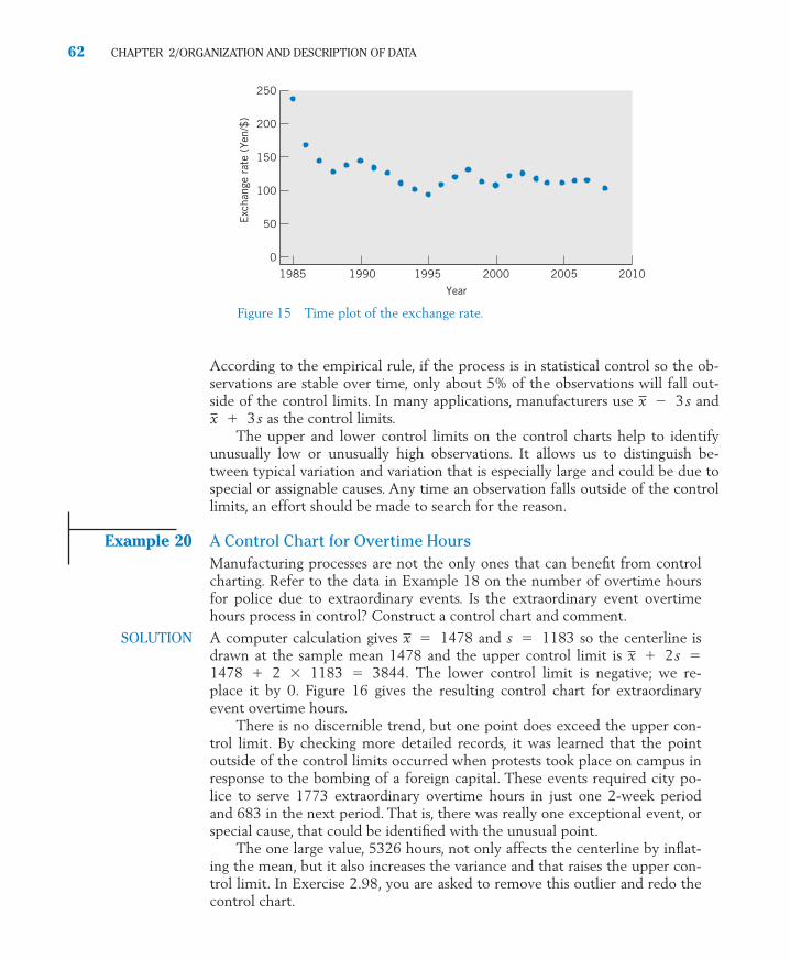
According to the empirical rule, if the process is in statistical control so the ob-servations are stable over time, only about 5% of the observations will fall out-side of the control limits. In many applications, manufacturers use and
as the control limits.The upper and lower control limits on the control charts help to identify
unusually low or unusually high observations. It allows us to distinguish be-tween typical variation and variation that is especially large and could be due tospecial or assignable causes. Any time an observation falls outside of the controllimits, an effort should be made to search for the reason.
Example 20 A Control Chart for Overtime HoursManufacturing processes are not the only ones that can benefit from controlcharting. Refer to the data in Example 18 on the number of overtime hoursfor police due to extraordinary events. Is the extraordinary event overtimehours process in control? Construct a control chart and comment.
SOLUTION A computer calculation gives and so the centerline isdrawn at the sample mean 1478 and the upper control limit is
The lower control limit is negative; we re-place it by 0. Figure 16 gives the resulting control chart for extraordinaryevent overtime hours.
There is no discernible trend, but one point does exceed the upper con-trol limit. By checking more detailed records, it was learned that the pointoutside of the control limits occurred when protests took place on campus inresponse to the bombing of a foreign capital. These events required city po-lice to serve 1773 extraordinary overtime hours in just one 2-week periodand 683 in the next period. That is, there was really one exceptional event, orspecial cause, that could be identified with the unusual point.
The one large value, 5326 hours, not only affects the centerline by inflat-ing the mean, but it also increases the variance and that raises the upper con-trol limit. In Exercise 2.98, you are asked to remove this outlier and redo thecontrol chart.
1478 � 2 � 1183 � 3844.x � 2s �
s � 1183x � 1478
x � 3sx � 3s
62 CHAPTER 2/ORGANIZATION AND DESCRIPTION OF DATA
250
200
150
100
50
0
1985 1990
Year
1995 2000
Exc
hang
e ra
te (
Yen/
$)
2005 2010
Figure 15 Time plot of the exchange rate.
c02a.qxd 10/15/09 12:02 PM Page 62

Exercises
6. CHECKING THE STABILITY OF THE OBSERVATIONS OVER TIME 63
0
1000
2000
3000
4000
5000
6000
Ove
rtim
e ho
urs
10 2 3 4 5 6 7 8 9 10 11 12 13 14 15 16
6-month periods
3844
1478
Figure 16 Control chart for extraordinary event overtime hours.
2.92 Make a time plot of the phone call data inExercise 2.48 and comment on the statisticalcontrol.
2.93 A city department has introduced a qualityimprovement program and has allowed em-ployees to get credit for overtime hours whenattending meetings of their quality groups.The total number of overtime meeting hoursfor each of the 26 pay periods in one year byrow were
30 215 162 97 194 163 60 41 10043 96 69 80 42 162 75 95 6557 131 54 114 64 114 38 140
Make a time plot of the overtime meetinghours data.
2.94 Make a control chart for the data referred to inExercise 2.92 and comment.
2.95 Make a control chart for the data in Exercise2.93 and comment.
2.96 The exchange rate between the United Statesand Canada can be stated as the number ofCanadian dollars that can be purchased with$1. The official values for the year are
1998 1999 2000 2001 2002 2003
1.48 1.49 1.48 1.55 1.57 1.40
2004 2005 2006 2007 2008
1.30 1.21 1.13 1.07 1.07
Year 1992 1993 1994 1995 1996 1997
Exchange rate 1.21 1.29 1.37 1.37 1.36 1.38
Is this exchange rate in statistical control?Make a time plot and comment.
2.97 Make a control chart of the data in Exercise2.96 and comment.
2.98 Make a control chart for the extraordinary eventovertime data in Example 18 after removing theoutlier identified in that example. You need torecalculate the mean and standard deviation.
c02a.qxd 10/15/09 12:02 PM Page 63

7. MORE ON GRAPHICS
The importance of graphing your data cannot be overemphasized. If a featureyou expect to see is not present in the plots, statistical analyses will be of noavail. Moreover, creative graphics can often highlight features in the data andeven give new insights.
The devastation of Napoleon’s Grand Army during his ill-fated attemptto capture Russia was vividly depicted by Charles Minard. The 422,000troops that entered Russia near Kaunas are shown as a wide (shaded) riverflowing toward Moscow and the retreating army as a small (black) stream.The width of the band indicates the size of the army at each location on themap. Even the simplified version of the original graphic, appearing in Figure 17,dramatically conveys the losses that reduced the army of 422,000 men to10,000 returning members. The temperature scale at the bottom, pertainingto the retreat, helps to explain the loss of life, including the incident wherethousands died trying to cross the Berezina River in subzero temperatures.(For a copy of Minard’s more detailed map and additional discussion, see E. R. Tufte, The Visual Display of Quantitative Information, Cheshire, CT:Graphics Press, 1983.)
64 CHAPTER 2/ORGANIZATION AND DESCRIPTION OF DATA
Kaunas422,000
10,000
Niemen R.Berezina R.
Smolensk
Moscow100,000
0˚ C–15˚–30˚
–9˚–21˚
–11˚–20˚
–30˚Dec. 6 Nov. 28 Nov. 14 Oct. 9 Temperature
Figure 17 The demise of Napoleon’s army in Russia, 1812–1813,based on Charles Minard.
Another informative graphic, made possible with modern software, is thedisplay of ozone by city in Figure 18. This figure illustrates improved air qual-ity relative to the previous year and the ten year average.
c02a.qxd 10/15/09 12:02 PM Page 64

Graphs can give a vivid overall picture.Dave Carpenter/Cartoon Stock
Figure 18 Ozone Season for 2008 compared to 2007 and ten year average.
7. MORE ON GRAPHICS 65
c02a.qxd 10/15/09 12:02 PM Page 65

66 CHAPTER 2/ORGANIZATION AND DESCRIPTION OF DATA
8. STATISTICS IN CONTEXT
The importance of visually inspecting data cannot be overemphasized. We present a mini-case study2 that shows the importance of first appropriately plotting and then monitoring manufacturing data. This statistical application con-cerns a ceramic part used in a popular brand of coffee makers. To make this ce-ramic part, a mixture of clay, water, and oil is poured into the cavity between twodies of a pressing machine. After pressing but before the part is dried to a hard-ened state, critical dimensions are measured. The depth of a slot is of interest here.
Sources of variation in the slot depth abound: the natural uncontrolled variationin the clay–water–oil mixture, the condition of the press, differences in operators,and so on. Some variation in the depth of the slot is inevitable. Even so, for the partto fit when assembled, the slot depth needs to be controlled within certain limits.
Every half hour during the first shift, slot depth is measured on three ce-ramic parts selected from production. Table 12 gives the data obtained on a Fri-day. The sample mean for the first sample of 218, 217, and 219 (thousandths ofinch) is ( 218 � 217 � 219 )/ 3 � 654/ 3 � 218, and so on.
TABLE 12 Slot Depth (thousandths of an inch)
Time 7:00 7:30 8:00 8:30 9:00 9:30 10:00
1 218 218 216 217 218 218 2192 217 218 218 220 219 217 2193 219 217 219 221 216 217 218
SUM 654 653 653 658 653 652 656218.0 217.7 217.7 219.3 217.7 217.3 218.7
Time 10:30 11:00 11:30 12:30 1:00 1:30 2:00 2:30
1 216 216 218 219 217 219 217 2152 219 218 219 220 220 219 220 2153 218 217 220 221 216 220 218 214
SUM 653 651 657 660 653 658 655 644217.7 217.0 219.0 220.0 217.7 219.3 218.3 214.7x
x
An x-bar chart will indicate when changes have occurred and there is aneed for corrective actions. Because there are 3 slot measurements at each time,it is the 15 sample means that are plotted versus time order. We will take thecenterline to be the mean of the 15 sample means, or
Centerline: x �218.0 � � � � � 214.7
15� 218.0
2Courtesy of Don Ermer.
c02b.qxd 10/15/09 12:03 PM Page 66

When each plotted mean is based on several observations, the variance can beestimated by combining the variances from each sample. The first sample has vari-ance (3 � 1)� 1.000 and so on. The details are not important, but a computer calculation of thevariance used to set control limits first determines the average of the 15 individualsample variances,
and, for reasons given in Chapter 7, divides by 3 to give the variance of a singlesample mean. That is, 1.58/ 3 � .527 is the appropriate s2. The control limitsare set at three times the estimated standard deviation .726, or3 � .726 � 2.2 units from the centerline.
Lower control limit: LCL � 218.0 � 2.2 � 215.8Upper control limit: UCL � 218.0 � 2.2 � 220.2
The x-bar chart is shown in Figure 19. What does the chart tell us?
s � √.527 �
1.000 � 0.333 � � � � � 0.33315
� 1.58
s 12 � [(218 � 218)2 � (217 � 218)2 � (219 � 218)2]/
8. STATISTICS IN CONTEXT 67
220
219
218
217
216
215
214
0 5
Sample number
Sam
ple
mea
n
10 15
221
UCL � 220.2
Mean � 218
LCL � 215.8
•
•
•
•
•
••
•
••
•
•
• ••
Figure 19 X-bar chart for depth.
The x-bar chart shows that the process was stable throughout the day andno points were out of control except the last sample. It was then that an unfor-tunate oversight occurred. Because it was near the end of her shift and the startof the weekend, the operator did not report the out-of-control value to eitherthe setup person or the foreman. She knew the setup person was already clean-ing up for the end of the shift and that the foreman was likely thinking aboutgoing across the street to the Legion Bar for some refreshments as soon as theshift ended. The operator did not want to ruin anyone’s weekend plans so shekept quiet.
c02b.qxd 10/15/09 12:03 PM Page 67

68 CHAPTER 2/ORGANIZATION AND DESCRIPTION OF DATA
When the pressing machine was started up on Monday morning, one of thedies broke. The cost of the die was over a thousand dollars. But, when a cus-tomer was called and told there would be a delay in delivering the ceramicparts, he canceled the order. Certainly the loss of a customer is an even more ex-pensive item.
Later, it was concluded that the clay had likely dried and stuck to the dieleading to the break. A problem was predicted by the chart on Friday. Althoughthe chart correctly indicated a problem at that time, someone had to act for themonitoring procedure to work.
USING STATISTICS WISELY
1. As a first step, always graph the data as a dot diagram or histogram to as-sess the overall pattern of data.
2. When comparing histograms based on different class intervals, be sure tocreate histograms whose height is relative frequency divided by widthof interval.
3. Calculate summary statistics to describe the data set. Always determinethe sample mean and standard deviation. The five-number summary
minimum first quartile median third quartile maximum
provides an additional summary when the sample sizes are moderatelylarge. It helps describe cases where the dot diagram or histogram has asingle long tail.
4. Use the median to describe the center when a small sample contains anextreme observation. The sample median is not influenced by a few verylarge or very small observations that may even be incorrectly recorded.
5. Do not routinely calculate summary statistics without identifying un-usual observations (outliers) which may have undue influence on thevalue of a summary statistic.
KEY IDEAS AND FORMULAS
Qualitative data refer to frequency counts in categories. These are summa-rized by calculating the
for the individual categories.The term numerical-valued variable or just variable refers to a characteristic
that varies over units and is measured on a numerical scale. Discrete variables
Relative frequency �Frequency
Total number of observations
c02b.qxd 10/15/09 12:03 PM Page 68

are usually counts and all discrete variables have gaps in their scale of measure-ment. Continuous variables, like height or weight, can conceptually take anyvalue in an interval. Data resulting from measurements of a variable are eitherdiscrete or continuous data.
For a discrete data set, the frequency is the count of the number of observa-tions having a distinct value. The relative frequency is the proportion of sampleunits having this property.
The discrete data set is summarized by a frequency distribution that lists thedistinct data points and their corresponding relative frequencies. Either a line di-agram or a histogram can be used for a graphical display.
Continuous measurement data should be graphed as a dot diagram whenthe data set is small, say, fewer than 20 or 25 observations. Larger data sets arefirst summarized in a frequency table. This is constructed by grouping the ob-servations in class intervals, preferably of equal lengths. The class intervals arenon-overlapping and cover the range of the data set from smallest to largest.We recommend specifying an endpoint convention that tells which of theclass boundaries, or endpoints of the class intervals, to include and which toexclude from each class interval. A list of the class intervals along with thecorresponding relative frequencies provides a frequency distribution whichcan graphically be displayed as a histogram. The histogram is constructed tohave total area 1, equal to total relative frequency. That is, for each class inter-val, we draw a rectangle whose area represents the relative frequency of theclass interval.
A stem-and-leaf display is another effective means of display when the dataset is not too large. It is more informative than a histogram because it retains theindividual observations in each class interval instead of lumping them into a fre-quency count. Two variants are the double-stem display and five-stem display.
Pareto diagrams display events according to their frequency in order tohighlight the most important few that occur most of the time.
A summary of measurement data (discrete or continuous) should also in-clude numerical measures of center and spread.
Two important measures of center are
Sample mean
Sample median
The quartiles and, more generally, percentiles are other useful locators of the distribution of a data set. The second quartile is the same as the median.The sample quartiles divide the ordered data into nearly four equal parts. The100p-th percentile has least proportion p at or below and proportion 1 – p at or above.
� middle most value of the ordered data set
x �� x
n
Relative frequency �Frequency
Total number of observations
KEY IDEAS AND FORMULAS 69
c02b.qxd 10/15/09 12:03 PM Page 69

70 CHAPTER 2/ORGANIZATION AND DESCRIPTION OF DATA
The amount of variation, or spread, of a data set is measured by the samplestandard deviation s. The sample variance s2 is given by
Also, (convenient for hand calculation)
Sample standard deviation
The standard deviation indicates the amount of spread of the data pointsaround the mean If the histogram appears symmetric and bell-shaped, thenthe interval
Two other measures of variation are
Sample range � Largest observation � Smallest observation
and
Sample interquartile range � Third quartile � First quartile
The five-number summary, namely, the median, the first and third quartiles,the smallest observation, and the largest observation, together serve as useful in-dicators of the distribution of a data set. These are displayed in a boxplot.
TECHNOLOGY
Creating graphs and computing statistical summaries have become considerablyeasier because of recent developments in software. In all our professional appli-cations of statistics, we begin by entering the data in a worksheet. We then readfrom the worksheet while another person checks against the original. This pro-cedure has eliminated many errors in data entry and allowed us to proceedknowing that the computer software is using the correct data.
In the technology sections of this text, we give the essential details for usingMINITAB, EXCEL, and the TI-84/ 83 Plus graphing calculator. The first two usethe worksheet format.
MINITAB
The MINITAB screen is split with the bottom part being the worksheet. In theexample here, we have typed sleep in the top entry and then in row 1 of the firstcolumn we have typed the first number of hours of sleep in Table 4. The rest ofthe hours of sleep are typed in the other cells in column 1.
x � 3s includes approximately 99.7% of the data
x � 2s includes approximately 95% of the data
includes approximately 68% of the data x � s
x.
s � �√s2
s2 �1
n � 1 �� x2 �
� � x �2
n �
s2 �� ( x � x )2
n � 1
c02b.qxd 10/15/09 12:03 PM Page 70

Alternatively, the data sets in the book are stored as MINITAB worksheetson the book’s Web site. Go to www.wiley.com/college/johnson and click on thisbook. For instance, the hours of sleep are in C2T4.mtw, indicating Table 4 ofChapter 2. To open this worksheet:
Under File choose Open Worksheet and go to the drive that contains thedownloaded files.Click on the MINITAB folder and then click on the file name C2T4. Click OK.
This will activate the worksheet in MINITAB and you do not have to manu-ally enter the numbers.
TECHNOLOGY 71
The summary statistics can be obtained by pulling down the menu in thetop bar under Stat, then choosing Basic Statistics and then Graphic Summary.More specifically,
Data in C1
Dialog box:Stat > Basic Statistics > Graphical Summary.Type C1 in Variables. Click OK.
c02b.qxd 10/15/09 12:03 PM Page 71

72 CHAPTER 2/ORGANIZATION AND DESCRIPTION OF DATA
MINITAB uses a slightly different definition of the quartiles and their valuesmay slightly differ from those calculated by the method in this book.
MINITAB will also create a histogram. With the data in C1,
Dialog box:
Graph > Histogram.Select Simple in Variables. Click OK.Type C1 in X. Click OK.
MINITAB will also create boxplots, dot plots, and stem-and-leaf displays.With the data in C1 ,
Dialog box:
Graph > Dotplot.Select Simple. Click OK.Type C1 in Graph variables. Click OK.
produces a dot plot. To obtain a boxplot, replace the first step by
Graph > Boxplot.
and to obtain a stem-and-leaf display, replace the first two steps by the single step
Graph > Stem-and-Leaf.
Clicking on Labels before the last OK will allow you to put titles on yourgraph.
EXCEL
Begin with the data in column A. For the hours of sleep from Table 4, thespread sheet is given on page 73.
Alternatively, the data sets in the book are stored in EXCEL workbooks onthe book’s Web site. Go to www.wiley.com/college/johnson and click on thisbook. For instance, the hours of sleep are in C2T4.xls, indicating Table 4 ofChapter 2. Go to the drive containing the downloaded files and click on theEXCEL folder and then on the file name C2T4. The workbook having the datafrom Table 4 will then open.
Most of the statistical procedures we will use start with
Select Tools and then Data Analysis.If Data Analysis is not listed, then it must be added once. To do so, selectTools then Add-Ins. Check Analysis Toolpak and click OK.
To obtain the summary statistics,
Select Tools, then Data Analysis, and then Descriptive Statistics.Click OK. Place cursor in the Input Range window and use the mouse tohighlight the data in column A. Check Summary Statistics and click OK.
c02b.qxd 10/15/09 12:03 PM Page 72

TI-84/83 PLUS
Press STAT, select 1:Edit, and then enter the data in L1.Press STAT, highlight Calc, and select 1:1–Var Stats.With 1�1–Var Stats in the Home screen, press 2nd 1�1–Var Stats 1 toinsert L1 on the Home screen.Then press ENTER.
9. REVIEW EXERCISES
9. REVIEW EXERCISES 73
Number of Workersin Millions
2007 2000
Goods producing 22.2 24.6Service (private) 115.4 107.1Government 22.2 20.8
Total 159.8 152.5
groups for the years 2000 and 2007. (Source:Statistical Abstract of the United States, 2009.)
(a) For each year, calculate the relative fre-quencies of the occupation groups.
(b) Comment on changes in the occupationpattern between 2000 and 2007.
2.100 Table 13 gives data collected from the studentsattending an elementary statistics course at theUniversity of Wisconsin. These data includesex, height, number of years in college, and thegeneral area of intended major [Humanities(H); Social Science (S); Biological Science (B);Physical Science (P)].
2.99 Recorded here are the numbers of civilians em-ployed in the United States by major occupation
c02b.qxd 10/15/09 12:03 PM Page 73

74 CHAPTER 2/ORGANIZATION AND DESCRIPTION OF DATA
(a) Summarize the data of “intended major”in a frequency table.
(b) Summarize the data of “year in college” ina frequency table and draw either a linediagram or a histogram.
2.101 Referring to Exercise 2.100, plot the dot dia-grams of heights separately for the male andfemale students and compare.
2.102 Refer to the data on power outages in TableD.1 in the Data Bank. Make a Pareto chart forthe cause of the outage.
2.103 The dollar amounts claimed by businessmenfor their lunches are to be grouped into thefollowing classes: 0–5, 5–10, 10–15, 15–20,20 or more. The left endpoint is included. Isit possible to determine from this frequency
distribution the exact number of lunches forwhich the amount claimed was:
(a) Less than 15?
(b) 10 or more?
(c) 30 or more?
2.104 Mung bean sprouts are more widely used inAsian cooking than the beans themselves. Tostudy their growth, an experimenter presoakedsome beans until they sprouted about 1 mil-limeter. Five were randomly selected andplaced in individual petri dishes. After 96hours, their lengths (mm)
143 131 101 143 111
were obtained. Find the mean and standarddeviation.
TABLE 13 Class Data
Student Height Year in Intended Student Height Year in IntendedNo. Sex in Inches College Major No. Sex in Inches College Major
1 F 67 3 S 26 M 67 1 B2 M 72 3 P 27 M 68 3 P3 M 70 4 S 28 M 72 4 B4 M 70 1 B 29 F 68 3 P5 F 61 4 P 30 F 66 2 B6 F 66 3 B 31 F 65 2 B7 M 71 3 H 32 M 64 4 B8 M 67 4 B 33 M 72 1 H9 M 65 3 S 34 M 67 4 B
10 F 67 3 B 35 M 73 3 S11 M 74 3 H 36 F 71 4 B12 M 68 3 S 37 M 71 3 B13 M 74 2 P 38 M 69 2 S14 F 64 4 P 39 F 69 4 P15 M 69 3 S 40 M 74 4 S16 M 64 3 B 41 M 73 3 B17 M 72 4 P 42 M 68 3 B18 M 71 3 B 43 F 66 2 S19 F 67 2 S 44 M 73 2 P20 M 70 4 S 45 M 73 2 S21 M 66 4 S 46 M 67 4 S22 F 67 2 B 47 F 62 3 S23 M 68 4 S 48 M 68 2 B24 M 71 3 H 49 M 71 3 S25 M 75 1 S
c02b.qxd 10/15/09 12:03 PM Page 74

2.105 The weights of twenty adult grizzly bears cap-tured and released are summarized in the com-puter output
Descriptive Statistics: bearwt
Variable N Mean Median StDevBearwt 20 227.4 232.5 82.7
(a) Locate two measures of center tendency,or location, and interpret the values.
(b) Locate the standard deviation.
(c) Calculate the z score for a grizzly bear thatweighs 320 pounds. See Exercise 2.82.
2.106 The stem-and-leaf display given here showsthe final examination scores of students in asociology course. (Leaf unit � 1.0)
9. REVIEW EXERCISES 75
(a) Find the median score.
(b) Find the quartiles and .
(c) What proportion of the students scoredbelow 70? 80 and over?
2.107 The following are the numbers of passengerson the minibus tour of Hollywood.
9 12 10 11 11 7 12 6 11 4 10 10 11 9 107 10 8 8 9 8 9 11 9 8 6 10 6 8 11
(a) Find the sample median.
(b) Find the sample mean.
(c) Find the sample variance.
2.108 The following table shows the age at inaugura-tion of each U.S. president.
(a) Make a stem-and-leaf display with a dou-ble stem.
(b) Find the median, and .Q3Q1
Q3Q1
Stem-and-LeafDisplay of Scores
2 573 2444 11795 033686 0124477 2235568998 004579 0036
Age atName Inauguration
1. Washington 572. J. Adams 613. Jefferson 574. Madison 575. Monroe 586. J. Q. Adams 577. Jackson 618. Van Buren 549. W. H. Harrison 68
10. Tyler 5111. Polk 4912. Taylor 6413. Fillmore 5014. Pierce 4815. Buchanan 6516. Lincoln 5217. A. Johnson 5618. Grant 4619. Hayes 5420. Garfield 4921. Arthur 5022. Cleveland 4723. B. Harrison 5524. Cleveland 5525. McKinley 5426. T. Roosevelt 4227. Taft 5128. Wilson 5629. Harding 5530. Coolidge 5131. Hoover 5432. F. D. Roosevelt 5133. Truman 6034. Eisenhower 6235. Kennedy 4336. L. Johnson 5537. Nixon 5638. Ford 6139. Carter 5240. Reagan 6941. G. Bush 6442. Clinton 4643. G. W. Bush 5444. Obama 47
c02b.qxd 10/15/09 12:03 PM Page 75

76 CHAPTER 2/ORGANIZATION AND DESCRIPTION OF DATA
2.109 (a) Calculate and s for the data 6, 8, 4, 9, 8.
(b) Consider the data set 106, 108, 104, 109,108, which is obtained by adding 100 toeach number given in part (a). Use yourresults of part (a) and the propertiesstated in Exercises 2.52 and 2.74 to ob-tain the and s for this modified data set.Verify your results by direct calculationswith this new data set.
(c) Consider the data set �18, �24, �12,�27, �24, which is obtained by multiply-ing each number of part (a) by �3. Re-peat the problem given in part (b) for thisnew data set.
2.110 Refer to the class data in Exercise 2.100. Cal-culate the following.
(a) and s for the heights of males.
(b) and s for the heights of females.
(c) Median and the quartiles for the heightsof males.
(d) Median and the quartiles for the heightsof females.
2.111 In a genetic study, a regular food was placed ineach of 20 vials and the number of flies of aparticular genotype feeding on each vialrecorded. The counts of flies were also recordedfor another set of 20 vials that contained grapejuice. The following data sets were obtained(courtesy of C. Denniston and J. Mitchell).
No. of Flies (Regular Food)15 20 31 16 22 22 23 33 38 2825 20 21 23 29 26 40 20 19 31
No. of Flies (Grape Juice)
6 19 0 2 11 12 13 12 5 162 7 13 20 18 19 19 9 9 9
(a) Plot separate dot diagrams for the twodata sets.
(b) Make a visual comparison of the two dis-tributions with respect to their centersand spreads.
(c) Calculate and s for each data set.
2.112 The data below were obtained from a detailedrecord of purchases of toothpaste over severalyears (courtesy of A. Banerjee). The usage
x
x
x
x
x times (in weeks) per ounce of toothpaste for ahousehold taken from a consumer panel were
.74 .45 .80 .95 .84 .82 .78 .82 .89 .75 .76 .81
.85 .75 .89 .76 .89 .99 .71 .77 .55 .85 .77 .87
(a) Plot a dot diagram of the data.
(b) Find the relative frequency of the usagetimes that do not exceed .80.
(c) Calculate the mean and the standard de-viation.
(d) Calculate the median and the quartiles.
2.113 To study how first-grade students utilize theirtime when assigned to a math task, a researcherobserves 24 students and records their timesoff-task out of 20 minutes. The dotplot appearson page 3. (courtesy of T. Romberg).
For this data set, find:
(a) Mean and standard deviation.
(b) Median.
(c) Range.
2.114 The following summary statistics were ob-tained from a data set.
Approximately what proportion of the obser-vations are:
(a) Below 96.0?
(b) Above 84.0?
(c) In the interval 59.5 to 101.5?
(d) In the interval 75.5 to 96.0?
(e) In the interval 49.0 to 112.0?
State which of your answers are based on theassumption of a bell-shaped distribution.
Q3 � 96.0
s � 10.5 Q1 � 75.5
x � 80.5 Median � 84.0
Times Off-Task (minutes)
4 0 2 2 4 14 6 9 7 2 75 4 13 7 7 10
10 0 5 3 9 8
c02b.qxd 10/15/09 12:03 PM Page 76

2.115 The 50 measurements of acid rain in Wiscon-sin, whose histogram is given on the coverpage of the chapter, are
3.58 3.80 4.01 4.01 4.05 4.054.12 4.18 4.20 4.21 4.27 4.284.30 4.32 4.33 4.35 4.35 4.414.42 4.45 4.45 4.50 4.50 4.504.50 4.51 4.52 4.52 4.52 4.574.58 4.60 4.61 4.61 4.62 4.624.65 4.70 4.70 4.70 4.70 4.724.78 4.78 4.80 5.07 5.20 5.265.41 5.48
(a) Calculate the median and quartiles.
(b) Find the 90th percentile.
(c) Determine the mean and standard devia-tion.
(d) Display the data in the form of a boxplot.
2.116 Refer to Exercise 2.115.
(a) Determine the intervals and
(b) What proportions of the measurementslie in those intervals?
(c) Compare your findings with the empiricalguidelines for bell-shaped distributions.
2.117 Refer to the earthquake size data in Exercise2.20.
(a) Calculate the median and quartiles.
(b) Calculate the mean and standard devia-tion.
(c) Display the data in the form of a boxplot.
2.118 The Dow Jones average provides an indicationof overall market level. The changes in this av-erage, from year end, from 1969 to 1970through 2007 to 2008 are summarized in thefollowing frequency table, where the left-handendpoint is excluded.
Yearly Changes in the Dow Jones Average
Change in DJ Average Frequency
(�4500, �1600] 1(�1600, �850] 1(�850, �250] 2
(�250, 0] 8(0, 250] 13
x � 3s.x � 2s,x � s,
9. REVIEW EXERCISES 77
(250, 850] 6(850, 1650] 5
(1650, 2450] 3
Total 39
(a) Calculate the relative frequency for theintervals.
(b) Plot the relative frequency histogram.(Hint: Since the intervals have unequalwidths, make the height of each rectangleequal to the relative frequency divided bythe width of the interval.)
(c) What proportion of the changes werenegative?
(d) Comment on the location and shape ofthe distribution.
2.119 The winning times of the men’s 400-meterfreestyle swimming in the Olympics (1964 to2008) appear in the following table.
Winning Times in Minutes and Seconds
Year Time
1964 4:12.21968 4:09.01972 4:00.271976 3:51.931980 3:51.311984 3:51.231988 3:46.951992 3:45.001996 3:47.972000 3:40.592004 3:43.102008 3:41.86
(a) Draw a dot diagram and label the pointsaccording to time order.
(b) Explain why it is not reasonable to groupthe data into a frequency distribution.
2.120 The mode of a collection of observations is de-fined as the observed value with largest relativefrequency. The mode is sometimes used as acenter value. There can be more than onemode in a data set. Find the mode for the datagiven in Exercise 2.13.
c02b.qxd 10/15/09 12:03 PM Page 77

78 CHAPTER 2/ORGANIZATION AND DESCRIPTION OF DATA
2.121 Lightning causes many deaths each year in theUnited States. The yearly number of deaths for50 years, 1959 through 2008 are, by rows,
183 129 149 153 165 129 149 110 88 129 131 122 12294 124 102 91 74 98 88 63 74 66 77 77 6774 68 88 68 67 74 73 41 43 69 85 53 4244 46 51 44 51 43 32 38 47 45 27
Obtain the mean and standard deviation.
2.122 With reference to the lightning data in Exercise2.121,
(a) Make a time plot of the data.
(b) Comment on the appropriateness of pre-senting the mean and standard deviationas summaries.
The Following Exercises Require a Computer.
Calculations of the descriptive statistics such as and sare increasingly tedious with larger data sets. Currentcomputer software programs alleviate the drudgery ofhand calculations. Use MINITAB or some other pack-age program.
2.123 Find x_
and s for:
(a) The lizard data in Exercise 2.19.
(b) The acid rain data in Exercise 2.115.
2.124 Lumber intended for building houses and otherstructures must be monitored for strength. Themeasurement of strength (pounds per squareinch) for 61 specimens of Southern Pine (Source:U.S. Forest Products Laboratory) yielded
4001 3927 3048 4298 4000 34454949 3530 3075 4012 3797 35504027 3571 3738 5157 3598 47494263 3894 4262 4232 3852 42563271 4315 3078 3607 3889 31473421 3531 3987 4120 4349 40713686 3332 3285 3739 35444103 3401 3601 3717 48465005 3991 2866 3561 40034387 3510 2884 3819 31733470 3340 3214 3670 3694
Using MINITAB, the sequence of choices
x
Data(in 2.126.txt):
Strength
Dialog box:
Stat Basic Statistics Graphical Summary.
Type Strength in Variables. Click OK.
produces a rather complete summary of thedata. It includes the output on page 79.
(a) Use this output to identify a departurefrom a bell-shaped pattern.
(b) MINITAB uses a slightly different schemeto determine the first and third quartiles,but the difference is not of practical impor-tance with large samples. Calculate the firstquartile using the definition in this bookand compare with the value in the output.
2.125 Find and s for the data set in Table 4.
2.126 Find and s for the final times to run 1.5 milesin Table D.5 in the Data Bank.
2.127 The SAS computer software package producedthe output on page 79. Compare the mean andstandard deviation with that of the MINITABoutput in Exercise 2.124. Which output givesmore digits?
2.128 The salmon fisheries support a primary indus-try in Alaska and their management is of highpriority. Salmon are born in freshwater riversand streams but then swim out into the oceanfor a few years before returning to spawn anddie. In order to identify the origins of maturefish, researchers studied growth rings on theirscales. The growth the first year in freshwateris measured by the width of the growth ringsfor that period of life. The growth ring for thefirst year in the ocean environment will give anindication of growth for that period. A set ofthese measurements are given in Table D.7 inthe Data Bank.
(a) Describe the freshwater growth for malesby making a histogram and calculating themean, standard deviation, and quartiles.
x
x
c02b.qxd 10/15/09 12:03 PM Page 78

9. REVIEW EXERCISES 79
3000 3600 4200
Summary for strength
4800
MeanStDevVarianceSkewnessKurtosisN
Minimum1st QuartileMedian3rd QuartileMaximum
3801.0513.5
263724.40.5773660.265812
61
2866.03457.53738.04087.05157.0
UNIVARIATE PROCEDURE
VARIABLE � X1MOMENTS
N 61 VARIANCE 263724.4MEAN 3800.951STD DEV 513.5411
QUANTILES (DEF � 5)
100% MAX 5157 99% 515775% Q3 4071 95% 484650% MED 3738 90% 434925% Q1 3470 10% 31730% MIN 2866 5% 3075
1% 2866RANGE 2291Q3–Q1 601
EXTREMES
LOWEST OBS HIGHEST OBS2866( 31) 4749( 28)2884( 42) 4846( 22)3048( 3) 4949( 12)3075( 14) 5005( 29)3078( 47) 5157( 26)
Figure 20 MINITAB output for Exercise 2.124.
Figure 21 SAS output for Exercise 2.125.
c02b.qxd 10/15/09 12:03 PM Page 79

80 CHAPTER 2/ORGANIZATION AND DESCRIPTION OF DATA
(b) Describe the freshwater growth for femalesby making a histogram and calculating themean, standard deviation, and quartiles.
(c) Construct boxplots to compare the growthof males and females.
2.129 Refer to the alligator data in Table D.11 of theData Bank. Using the data on for thirty-seven alligators:
(a) Make a histogram.
(b) Obtain the sample mean and standard de-viation.
2.130 Refer to Exercise 2.129.
(a) Obtain the quartiles.
x5
(b) Obtain the 90th percentile. How many ofthe alligators above the 90th percentileare female?
2.131 Refer to the data on malt extract in Table D.8of the Data Bank.
(a) Obtain sample mean and standard devia-tion.
(b) Obtain quartiles.
(c) Check conformity with the empiricalrule.
c02b.qxd 10/15/09 12:03 PM Page 80

1. Introduction2. Summarization of Bivariate Categorical Data3. A Designed Experiment for Making a Comparison4. Scatter Diagram of Bivariate Measurement Data5. The Correlation Coefficient—
A Measure of Linear Relation6. Prediction of One Variable from Another
(Linear Regression)7. Review Exercises
3
Descriptive Study of Bivariate Data
c03.qxd 10/15/09 10:59 AM Page 81

Hydrogen–Carbon Association in Moon Rocks
00
20
50
70
100
Car
bon
(ppm
)
25 50 75Hydrogen (ppm)
Content of moon rocks
100 125
In their quest for clues to the origin and composition of the planets, scientistsperformed chemical analyses of rock specimens collected by astronauts and un-manned space probes. The Apollo moon landings made it possible to study first-hand the geology of the moon. Eleven lunar rocks were analyzed for carbon andhydrogen content.
Rocks with large amounts of hydrogen tend to have large amounts of carbon.Other rocks tend to have small amounts of both elements, indicating a positiveassociation between hydrogen and carbon content.
© Photo Researchers.
c03.qxd 10/15/09 10:59 AM Page 82

1. INTRODUCTION
In Chapter 2, we discussed the organization and summary description of dataconcerning a single variable. Observations on two or more variables are oftenrecorded for the individual sampling units; the height and weight of individuals,or the number of goals scored by and against a team. By studying such bivariateor multivariate data, one typically wishes to discover if any relationships existbetween the variables, how strong the relationships appear to be, and whetherone variable of primary interest can be effectively predicted from informationon the values of the other variables. To illustrate the concepts, we restrict our at-tention to the simplest case where only two characteristics are observed on theindividual sampling units. Some examples are:
Gender and the type of occupation of college graduates.
Smoking habit and lung capacity of adult males.
Average daily carbohydrate intake and protein intake of 10-year-old children.
The age of an aircraft and the time required for repairs.
The two characteristics observed may both be qualitative traits, both numer-ical variables, or one of each kind. For brevity, we will only deal with situationswhere the characteristics observed are either both categorical or both numerical.Summarization of bivariate categorical data is discussed in Section 2. Sections 4,5, and 6 are concerned with bivariate measurement data and treat such issues asgraphical presentations, examination of relationship, and prediction of one vari-able from another.
2. SUMMARIZATION OF BIVARIATE CATEGORICAL DATA
When two traits are observed for the individual sampling units and each trait isrecorded in some qualitative categories, the resulting data can be summarized inthe form of a two-way frequency table. The categories for one trait are markedalong the left margin, those for the other along the upper margin, and the fre-quency counts recorded in the cells. The total frequency for any row is given inthe right-hand margin and those for any column given at the bottom margin.Both are called marginal totals.
Data in this summary form are commonly called cross-classified or cross-tabulated data. In statistical terminology, they are also called contingency tables.
Example 1 Calculation of Relative Frequencies Aids InterpretationFour hundred undergraduates were surveyed concerning their part-time workduring the semester. The number of hours worked last week was categorizedas: worked 10 or few hours, worked more than 10 hours, or did not work.The students were also categorized as underclassman or upperclassman. Thecross-tabulated frequency counts are presented as Table 1.
2. SUMMARIZATION OF BIVARIATE CATEGORICAL DATA 83
c03.qxd 10/15/09 10:59 AM Page 83

The entries of this table are self-explanatory. For instance, of the 400 studentspolled, 180 were underclassman. Among these, 132 did not work, 28 worked 10hours or less, and 20 worked more than 10 hours. To gain further understandingof how the responses are distributed, calculate the relative frequencies.
SOLUTION For this purpose, we divide each cell frequency by the sample size 400. Therelative frequencies, for instance 44/ 400 � .11, are shown in Table 2.
84 CHAPTER 3/DESCRIPTIVE STUDY OF BIVARIATE DATA
TABLE 1 Cross-Tabulated Frequency Counts of Work Hours
Work 10 Work MoreNo Job Hours or Less Than 10 Hours Total
Underclassman 132 28 20 180Upperclassman 124 44 52 220
Total 256 72 72 400
TABLE 2 Relative Frequencies for the Data of Table 1
Work 10 Work MoreNo Job Hours or Less Than 10 Hours Total
Underclassman .33 .07 .05 .45Upperclassman .31 .11 .13 .55
Total .64 .18 .18 1.00
TABLE 3 Relative Frequencies by Class
Work 10 Work MoreNo Job Hours or Less Than 10 Hours Total
Underclassman .733 .156 .111 1.000Upperclassman .564 .200 .236 1.000
Depending on the specific context of a cross-tabulation, one may also wish toexamine the cell frequencies relative to a marginal total. In Example 1, you maywish to compare the pattern of part-time work for underclassmen with that ofthe upperclassman. This is accomplished by calculating the relative frequenciesseparately for the two groups. For instance, 44/220 � .200, as Table 3 shows.
From the calculations presented in Table 3, it appears that a larger pro-portion of upperclassmen hold part-time jobs and that they tend to workmore than 10 hours a week.
Now the pertinent question is: Can these observed differences be ex-plained by chance or are there real differences in the pattern of part-timework between the populations of the two classes? We will pursue this aspectof statistical inference in Chapter 13.
c03.qxd 10/15/09 10:59 AM Page 84

SIMPSON’S PARADOX
Quite surprising and misleading conclusions can occur when data from differentsources are combined into a single table. We illustrate this reversal of implica-tions with graduate school admissions data.
Example 2 Combining Tables Can Produce Misleading SummariesWe consider graduate school admissions at a large midwestern university but,to simplify, we use only two departments as the whole school. We are inter-ested in comparing admission rates by gender and obtain the data in Table 4for the school.
Does there appear to be a gender bias?
SOLUTION It is clear from these admissions statistics that the proportion of males ad-mitted, 233/ 557 � .418, is greater than the proportion of females admit-ted, 88/ 282 � .312.
Does this imply some type of discrimination? Not necessarily. By checkingthe admission records, we were able to further categorize the cases accordingto department in Table 5. Table 4 is the aggregate of these two sets of data.
One of the two departments, mechanical engineering, has mostly male appli-cants. Even so, the proportion of males admitted, 151 / 186 � .812, is smaller
2. SUMMARIZATION OF BIVARIATE CATEGORICAL DATA 85
TABLE 4 School Admission Rates
Admit Not Admit Total Applicants
Male 233 324 557Female 88 194 282
Total 321 518 839
TABLE 5 Admission Rates by Department
Mechanical Engineering History
Not NotAdmit Admit Total Admit Admit Total
Male 151 35 186 Male 82 289 371Female 16 2 18 Female 72 192 264
Total 167 37 204 Total 154 481 635
c03.qxd 10/15/09 10:59 AM Page 85

than the proportion of females admitted, 16/18 � .889. The same is true forthe history department where the proportion of males admitted, 82/371 �.221, is again smaller than the proportion of females admitted, 72/264 �.273. When the data are studied department by department, the reverse butcorrect conclusion holds; females have a higher admission rate in both cases!
To obtain the correct interpretation, these data need to be presented asthe full three-way table of gender-admission action-department as givenabove. If department is ignored as in Table 4, and the data aggregated acrossthis variable, “department” can act as an unrecorded or lurking variable. In thisexample, it has reversed the direction of possible gender bias and led to the er-roneous conclusion that males have a higher admission rate than females.
The reversal of the comparison, such as in Example 2, when data are com-bined from several groups is called Simpson’s paradox.
When data from several sources are aggregated into a single table, there isalways the danger that unreported variables may cause a reversal of the findings.In practical applications, there is not always agreement on how much effort toexpend following up on unreported variables. When comparing two medicaltreatments, the results often need to be adjusted for the age, gender, and some-times current health of the subjects and other variables.
Exercises
86 CHAPTER 3/DESCRIPTIVE STUDY OF BIVARIATE DATA
Degree of Nausea
None Slight Moderate Severe Total
Pill 43 36 18 3 100Placebo 19 33 36 12 100
Total
3.1 Nausea from air sickness affects some travelers.A drug company, wanting to establish the effec-tiveness of its motion sickness pill, randomlygives either its pill or a look-alike sugar pill(placebo) to 200 passengers.
3.2 Breakfast cereals from three leading manufactur-ers can be classified either above average or be-low average in sugar content. Data for ten cere-als from each manufacturer are given below:
(a) Complete the marginal totals.
(b) Calculate the relative frequencies sepa-rately for each row.
(c) Comment on any apparent differences inresponse between the pill and the placebo.
Below Average Above Average Total
General Mills 3 7 10Kellogg’s 4 6 10Quaker 6 4 10
Total
(a) Complete the marginal totals.
(b) Calculate the relative frequencies sepa-rately for each row.
(c) Comment on any apparent differences be-tween the cereals produced by the threecompanies.
c03.qxd 10/15/09 10:59 AM Page 86

Male Female
English 23 19Computer Science 27 5
3.6 Interviews with 150 persons engaged in a stress-ful occupation revealed that 57 were alcoholics,64 were mentally depressed, and 42 were both.
(a) Based on these records, complete the fol-lowing two-way frequency table.
(b) Calculate the relative frequencies.
3.7 Cross-tabulate the “Class data” of Exercise 2.100according to gender (M, F) and the general areasof intended major (H, S, B, P). Calculate the rel-ative frequencies.
3.8 A psychologist interested in obese children gath-ered data on a group of children and their parents.
(a) Calculate the marginal totals.
(b) Convert the frequencies to relative fre-quencies.
(c) Calculate the relative frequencies sepa-rately for each row.
3.9 Typically, there is a gender unbalance amongtenured faculty, especially in the sciences. At alarge university, tenured faculty members in twodepartments, English and Computer Science,were categorized according to gender.
3.3 At the conclusion of one semester, a sample of250 juniors was questioned about how muchthey had studied for each of their final exams.Students were also classified as social science, bio-logical, or physical science majors.
Compare the times studying for finals by calcu-lating the relative frequencies.
3.4 A survey was conducted to study the attitudes ofthe faculty, academic staff, and students in regardto a proposed measure for reducing the heatingand air-conditioning expenses on campus.
Compare the attitude patterns of the threegroups by computing the relative frequencies.
3.5 Groundwater from 19 wells was classified as lowor high in alkalinity and low or high in dissolvediron. There were 9 wells with high alkalinity, 7that were high in iron, and 5 that were high inboth.
(a) Based on these data, complete the follow-ing two-way frequency table.
(b) Calculate the relative frequencies of thecells.
(c) Calculate the relative frequencies sepa-rately for each row.
2. SUMMARIZATION OF BIVARIATE CATEGORICAL DATA 87
Number of Hours of Study for Each Final
Major 10 or less More than10
Biological 30 45Physical 15 35Social 65 60
Favor Indifferent Opposed Total
Faculty 36 42 122 200Academic staff 44 77 129 250Students 106 178 116 400
Iron
Alkalinity Low High
LowHigh
Alcoholic Not Alcoholic Total
DepressedNot depressed
Total
Child
Parent Obese Not Obese
At least one obese 12 24Neither obese 8 36
(a) Calculate relative frequencies separatelyfor each row.
(b) Comment on major differences in the pat-terns for the two rows.
c03.qxd 10/15/09 10:59 AM Page 87

3.10 A large research hospital and a community hos-pital are located in your area. The surgeryrecords for the two hospitals are:
The outcome is “survived” if the patient lives atleast six weeks.
(a) Calculate the proportion of patients thatsurvive surgery at each of the hospitals.
(b) Which hospital do these data suggest youshould choose for surgery?
88 CHAPTER 3/DESCRIPTIVE STUDY OF BIVARIATE DATA
Died Survived Total
Research hospital 90 2110 2200Community hospital 23 677 700
3.11 Refer to Exercise 3.10. Not all surgery cases, evenof the same type, are equally serious. Large re-search hospitals tend to get the most serioussurgery cases, whereas community hospitals tendto get more of the routine cases. Suppose that pa-tients can be classified as being in either “Good” or“Poor” condition and the outcomes of surgery areas shown in table below.(a) Calculate the proportions that survive for
each hospital and each condition.(b) From these data, which hospital would you
choose if you were in good condition? Ifyou were in bad condition?
(c) Compare your answer with that toExercise 3.10. Explain this reversal as anexample of Simpson’s paradox and identifythe lurking variable in Exercise 3.10.
3. A DESIGNED EXPERIMENT FOR MAKING A COMPARISON
We regularly encounter claims that, as a group, smokers have worse health recordsthan nonsmokers with respect to one disease or another or that a new medical treat-ment is better than the former one. Properly designed experiments can often providedata that are so conclusive that a comparison is clear-cut. An example of a compara-tive study will illustrate the design issue and how to conduct an experiment.
During the early development of a medicated skin patch to help smokers breakthe habit, a test was conducted with 112 volunteers. The experimenters wanted toavoid errorneous conclusions caused by the so-called placebo effect when a treat-ment, with no therapeutic value, is administered to a subject but their symptoms im-prove anyway. One explanation is the positive thinking of subjects having high ex-pectations of getting better and who believe the real treatment will work.Consequently, half the volunteers were given an unmedicated skin patch.The data willconsist of a count of the number of persons who are abstinent at the end of the study.
Purpose: To determine the effectiveness of a medicated nicotine patchfor smoking cessation based on the end-of-therapy numbers of abstinentpersons in the medicated and unmedicated groups.
Survival Rates by Condition
Good Condition Poor Condition
Died Survived Total Died Survived Total
Research hospital 15 685 700 Research hospital 75 1425 1500Community hospital 16 584 600 Community hospital 7 93 100
Total 31 1269 1300 Total 82 1518 1600
c03.qxd 10/15/09 10:59 AM Page 88

What is involved in comparing two approaches or methods for doing some-thing? First the subjects, or experimental units, must be assigned to the two groupsin such a manner that neither method is favored. One approach is to list the sub-jects’ names on a piece of paper, cut the paper into strips, each with one name onit, and then draw one at a time until half the names are drawn. Ideally, we like tohave groups of equal size, so if there is an odd number of subjects, draw just overone-half. These subjects are assigned to the first approach. The other subjects areassigned to the second approach. This step, called random assignment, helps guar-antee a valid comparison. Any subject likely to respond positively has the samechance of supporting the first approach as supporting the second approach. Whensubjects cannot be randomly assigned, we will never know if observed differencesin the number of abstinent smokers is due to the approaches or some other vari-ables associated with the particular persons assigned to the two groups.
Subjects were randomly assigned to the medicated or unmedicated(placebo) groups. They were not told which group. As with many medical trials,this was a double blind trial. That is, the medical staff in contact with the pa-tients was also kept unaware of which patients were getting the treated patchand which were not. At the end of the study, the number of persons in eachgroup who were abstinent and who were smoking were recorded.
The data1 collected from this experiment are summarized in Table 6.
The proportion abstinent is 21/ 57 � .368 for the medicated skin patchgroup and only 11/ 55 � .200 for the control. The medicated patch seems towork. Later, in Chapter 10, we verify that the difference .368 � .200 � .168is greater than can be explained by chance variation.
In any application where the subjects might learn from the subjects beforethem, it would be a poor idea to perform all the trials for treatment 1 and thenall those for treatment 2. Learning or other uncontrolled variables must not begiven the opportunity to systematically affect the experiment. We could num-ber the subjects 1 to 112 and write each of these numbers on a separate slip ofpaper. The 112 slips of paper should be mixed and then drawn one at a time todetermine the sequence in which the trials are conducted.
Researchers continue to investigate the effectiveness of patches. One studypresents evidence against the effectiveness of patches.2
3. A DESIGNED EXPERIMENT FOR MAKING A COMPARISON 89
TABLE 6 Quitting Smoking
Abstinent Smoking
Medicated patch 21 36 57Unmedicated patch 11 44 55
32 80 112
1 M. Fiore, S. Kenford, D. Jorenby, D. Wetter, S. Smith, and T. Baker. “Two Studies of the Clinical Effectiveness of the Nicotine Patch with Different Counseling Treatments.” Chest 105 (1994),pp. 524–533.2A. Albert, et al. “Nicotine replacement therapy use among a cohort of smokers,” Journal of AddictiveDiseases 24(1) (2005), pp. 101–113.
c03.qxd 10/15/09 10:59 AM Page 89

3.12 With reference to the quit-smoking experiment,suppose two new subjects are available. Explainhow you would assign one subject to receive theplacebo and one to receive the medicated patch.
3.13 With reference to the quit-smoking experiment:
(a) Suppose the placebo trials were ignoredand you were only told that 21 of 57 were
90 CHAPTER 3/DESCRIPTIVE STUDY OF BIVARIATE DATA
abstinent after using the medicated patches.Would this now appear to be stronger evi-dence in favor of the patches?
(b) Explain why the placebo trials provide amore valid reference for results of the med-icated patch trials.
Exercises
4. SCATTER DIAGRAM OF BIVARIATE MEASUREMENT DATA
We now turn to a description of data sets concerning two variables, each mea-sured on a numerical scale. For ease of reference, we will label one variable xand the other y. Thus, two numerical observations (x, y) are recorded for eachsampling unit. These observations are paired in the sense that an (x, y) pairarises from the same sampling unit. An x observation from one pair and an x ory from another are unrelated. For n sampling units, we can write the measure-ment pairs as
The set of x measurements alone, if we disregard the y measurements, con-stitutes a data set for one variable. The methods of Chapter 2 can be employedfor descriptive purposes, including graphical presentation of the pattern of dis-tribution of the measurements, and calculation of the mean, standard deviation,and other quantities. Likewise, the y measurements can be studied disregardingthe x measurements. However, a major purpose of collecting bivariate data is toanswer such questions as:
Are the variables related?
What form of relationship is indicated by the data?
Can we quantify the strength of their relationship?
Can we predict one variable from the other?
Studying either the x measurements by themselves or the y measurements bythemselves would not help answer these questions.
An important first step in studying the relationship between two variables is tograph the data. To this end, the variable x is marked along the horizontal axis and yon the vertical axis on a graph paper. The pairs (x, y) of observations are then plot-ted as dots on the graph. The resulting diagram is called a scatter diagram or scat-ter plot. By looking at the scatter diagram, a visual impression can be formed aboutthe relation between the variables. For instance, we can observe whether the pointsband around a line or a curve or if they form a patternless cluster.
( x1 , y1 ), ( x2 , y 2 ), � � � , ( xn , yn )
c03.qxd 10/15/09 10:59 AM Page 90

Example 3 A Scatter Diagram Provides a Visual Display of a RelationshipRecorded in Table 7 are the data of
and
Score in the Graduate Management Aptitude Test (GMAT)
for applicants seeking admission to an MBA program.Construct a scatter diagram.
SOLUTION The scatter diagram is plotted in Figure 1. The southwest-to-northeast pat-tern of the points indicates a positive relation between x and y. That is, theapplicants with a high GPA tend to have a high GMAT. Evidently, the rela-tion is far from a perfect mathematical relation.
When the two measurements are made on two or more groups, visualcomparisons between groups are made by plotting the points on the samescatter plot. A different symbol is used for each group. The resulting graph iscalled a multiple scatter plot where “multiple” refers to groups.
y �
x � Undergraduate GPA
4. SCATTER DIAGRAM OF BIVARIATE MEASUREMENT DATA 91
TABLE 7 Data of Undergraduate GPA x and GMAT Score y
x y x y x y
3.63 447 2.36 399 2.80 4443.59 588 2.36 482 3.13 4163.30 563 2.66 420 3.01 4713.40 553 2.68 414 2.79 4903.50 572 2.48 533 2.89 4313.78 591 2.46 509 2.91 4463.44 692 2.63 504 2.75 5463.48 528 2.44 336 2.73 4673.47 552 2.13 408 3.12 4633.35 520 2.41 469 3.08 4403.39 543 2.55 538 3.03 419
3.00 509
700
GM
AT
600
500
400
300
2 3GPA
4
Figure 1 Scatter diagram of applicants’ scores.
c03.qxd 10/15/09 10:59 AM Page 91

Example 4 A Multiple Scatter Diagram for Visually Comparing RelationshipsConcern was raised by environmentalists that spills of contaminants were af-fecting wildlife in and around an adjacent lake. Estrogenic contaminants inthe environment can have grave consequences on the ability of living thingsto reproduce. Researchers examined the reproductive development of youngmale alligators hatched from eggs taken from around (1) Lake Apopka, thelake which was contaminated, and (2) Lake Woodruff, which acted as a con-trol. The contaminants were thought to influence sex steroid concentrations.The concentrations of two steroids, estradiol and testosterone, were deter-mined by radioimmunoassay.
Lake Apopka
Estradiol 38 23 53 37 30
Testosterone 22 24 8 6 7
Lake Woodruff
Estradiol 29 64 19 36 27 16 15 72 85
Testosterone 47 20 60 75 12 54 33 53 100
(a) Make a scatter diagram of the two concentrations for the Lake Apopkaalligators.
(b) Create a multiple scatter diagram by adding to the same plot the pairsof concentrations for the Lake Woodruff male alligators. Use a differentsymbol for the two lakes.
(c) Comment on any major differences between the two groups of malealligators.
92 CHAPTER 3/DESCRIPTIVE STUDY OF BIVARIATE DATA
50
100
Test
oste
rone
25 500 75
Estradiol
(a) Scatter diagram for Lake Apopka
A A
A A A
c03.qxd 10/15/09 10:59 AM Page 92

SOLUTION (a) Figure 2a gives the scatter diagram for the Lake Apopka alligators.
(b) Figure 2b is the multiple scatter diagram with the points for LakeWoodruff marked as B.
(c) The most prominent feature of the data is that the male alligators fromthe contaminated lake have, generally, much lower levels of testosteronethan those from the nearly pollution-free control lake. (The A’s are atthe bottom third of the multiple scatter diagram.) Low testosterone lev-els in males have grave consequences regarding reproduction.
5. THE CORRELATION COEFFICIENT—A MEASURE OF LINEAR RELATION
The scatter diagram provides a visual impression of the nature of the relationbetween the x and y values in a bivariate data set. In a great many cases, thepoints appear to band around a straight line. Our visual impression of the close-ness of the scatter to a linear relation can be quantified by calculating a numeri-cal measure, called the correlation coefficient.
The correlation coefficient, denoted by r, is a measure of strength of the lin-ear relation between the x and y variables. Before introducing its formula, weoutline some important features of the correlation coefficient and discuss themanner in which it serves to measure the strength of a linear relation.
1. The value of r is always between �1 and �1.
2. The magnitude of r indicates the strength of a linear relation, whereasits sign indicates the direction. More specifically,
5. THE CORRELATION COEFFICIENT—A MEASURE OF LINEAR RELATION 93
Figure 2 Scatter diagrams. A � Lake Apopka.B � Lake Woodruff.
50
100
Test
oste
rone
25 500 75
Estradiol
(b) Multiple scatter diagram
B
B
BB
BB
B A
BA
A
A A
B
c03.qxd 10/15/09 10:59 AM Page 93

if the pattern of (x, y) values is a band that runs fromlower left to upper right.
if the pattern of (x, y) values is a band that runs from up-per left to lower right.
if all (x, y) values lie exactly on a straight line with a posi-tive slope (perfect positive linear relation).
if all (x, y) values lie exactly on a straight line with a nega-tive slope (perfect negative linear relation).
A high numerical value of r, that is, a value close to �1 or �1, repre-sents a strong linear relation.
3. A value of r close to zero means that the linear association is very weak.
The correlation coefficient is close to zero when there is no visible patternof relation; that is, the y values do not change in any direction as the x valueschange. A value of r near zero could also happen because the points band
r � �1
r � �1
r � 0
r � 0
94 CHAPTER 3/DESCRIPTIVE STUDY OF BIVARIATE DATA
Figure 3 Correspondence between the values of r and the amount of scatter.
(a) r = .9 (b) r = .5 (c) r = –.5
(d ) r = –.9 (e) r = 0 (f ) r = 0
c03.qxd 10/15/09 10:59 AM Page 94

around a curve that is far from linear. After all, r measures linear association, anda markedly bent curve is far from linear.
Figure 3 shows the correspondence between the appearance of a scatter dia-gram and the value of r. Observe that (e) and ( f ) correspond to situationswhere The zero correlation in (e) is due to the absence of any relationbetween x and y, whereas in ( f ) it is due to a relation following a curve that isfar from linear.
CALCULATION OF r
The sample correlation coefficient quantifies the association between two nu-merically valued characteristics. It is calculated from n pairs of observations onthe two characteristics
The correlation coefficient is best interpreted in terms of the standardized ob-servations, or sample z values
where and the subscript x on s distin-guishes the sample standard deviation of the x observations from the samplestandard deviation of the y observations.
Since the difference has the units of x and the sample standard de-viation also has the same units, the standardized observation is free of theunits of measurements. The sample correlation coefficient is the sum of theproducts of the standardized x observation times the standardized y observa-tions divided by
When the pair has both components above their sample means or bothbelow their sample means, the product of standardized observations will be posi-tive; otherwise it will be negative. Consequently, if most pairs have both compo-nents simultaneously above or simultaneously below their means, r will be positive.
An alternative formula for r is used for calculation. It is obtained by cancel-ing the common term n � 1.
( xi , yi
)
n � 1.
sx
x i � xsy
sx � √�ni � 1 ( xi � x )2/ ( n � 1 )
Observation � Sample meanSample standard deviation
�xi � x
sx
( x1 , y1 ), ( x2 , y2
), � � � , ( xn , yn )
r � 0.
5. THE CORRELATION COEFFICIENT—A MEASURE OF LINEAR RELATION 95
Sample Correlation Coefficient
r �1
n � 1 �
n
i � 1 � xi � x
sx� � yi � y
sy�
c03.qxd 10/15/09 10:59 AM Page 95

The quantities and are the sums of squared deviations of the x observa-tions and the y observations, respectively. is the sum of cross products of thex deviations with the y deviations. This formula will be examined in more detailin Chapter 11.
Example 5 Calculation of Sample CorrelationCalculate r for the n � 4 pairs of observations
(2, 5) (1, 3) (5, 6) (0, 2)
SOLUTION We first determine the mean and deviations and then and the devi-ations See Table 8.
Consequently,
The value .930 is large and it implies a strong association where both x and ytend to be small or both tend to be large.
It is sometimes convenient, when using hand-held calculators, to evaluate rusing the alternative formulas for , , and (see Appendix A1.2).SxySyySxx
r �Sxy
√Sxx √Syy
�11
√14 √10� .930
y � y.yx � xx
Sxy
SyySxx
96 CHAPTER 3/DESCRIPTIVE STUDY OF BIVARIATE DATA
Calculation Formula for the Sample Correlation Coefficient
where
Sxx � � ( x � x )2 Syy � � ( y � y )2
Sxy � � ( x � x )( y � y )
r �Sxy
√Sxx √Syy
TABLE 8 Calculation of r
x y
2 5 0 1 0 1 01 3 �1 �1 1 1 15 6 3 2 9 4 60 2 �2 �2 4 4 4
Total 8 16 0 0 14 10 11SxySyySxxy � 4x � 2
( x � x )( y � y )( y � y )2( x � x )2y � yx � x
c03.qxd 10/15/09 10:59 AM Page 96

This calculation is illustrated in Table 9.
r �
43 �8 � 16
4
�30 �82
4 �74 �
(16)2
4
� .930
Sxy � � x y �� � x � � � y �
n
Sxx � � x2 �� � x �2
n Syy � � y2 �
� � y �2
n
5. THE CORRELATION COEFFICIENT—A MEASURE OF LINEAR RELATION 97
TABLE 9 Alternate Calculation of r
x y x2 y2 x y
2 5 4 25 101 3 1 9 35 6 25 36 300 2 0 4 0
Total 8 16 30 74 43� x � y � x2 � y2 � x y
Figure 4 r is not appropriate—samplesfrom two populations.
We remind the reader that r measures the closeness of the pattern of scatter toa line. Figure 3f on page 94 presents a strong relationship between x and y, but onethat is not linear. The small value of r for these data does not properly reflect thestrength of the relation. Clearly, r is not an appropriate summary of a curved pat-tern. Another situation where the sample correlation coefficient r is not appropri-ate occurs when the scatter plot breaks into two clusters. Faced with separate clus-ters as depicted in Figure 4, it is best to try and determine the underlying cause. Itmay be that a part of the sample has come from one population and a part fromanother.
c03.qxd 10/15/09 10:59 AM Page 97

CORRELATION AND CAUSATION
Data analysts often jump to unjustified conclusions by mistaking an observedcorrelation for a cause-and-effect relationship. A high sample correlation coeffi-cient does not necessarily signify a causal relation between two variables. A clas-sic example concerns an observed high positive correlation between the numberof storks sighted and the number of births in a European city. It is hoped no onewould use this evidence to conclude that storks bring babies or, worse yet, thatkilling storks would control population growth.
The observation that two variables tend to simultaneously vary in a certain di-rection does not imply the presence of a direct relationship between them. If werecord the monthly number of homicides x and the monthly number of religiousmeetings y for several cities of widely varying sizes, the data will probably indicatea high positive correlation. It is the fluctuation of a third variable (namely, the citypopulation) that causes x and y to vary in the same direction, despite the fact thatx and y may be unrelated or even negatively related. Picturesquely, the third vari-able, which in this example is actually causing the observed correlation betweencrime and religious meetings, is referred to as a lurking variable. The false correla-tion that it produces is called a spurious correlation. It is more a matter of com-mon sense than of statistical reasoning to determine if an observed correlation hasa practical interpretation or is spurious.
When using the correlation coefficient as a measure of relationship, wemust be careful to avoid the possibility that a lurking variable is affecting any ofthe variables under consideration.
Example 6 Spurious Correlation Caused by Lurking VariablesFigure 5 gives a scatter diagram of the number of person in prison, understate or federal jurisdiction, and the number of cell phone subscribers in eachof 10 years. Both variables are measured in millions (see Exercise 3.29).
This plot exhibits a pattern of strong positive correlation; the numericalvalue r = .987. Would restricting the number of cell phones result in fewerpersons in prison?
SOLUTION The scatter diagram reveals a strong positive correlation, but common sensesuggests there is no cause-and-effect relation to tie an increase in the numberof cell phone subscribers to an increase in the prison population. Realistically,the two variables should not have a causal relationship.
In Figure 6 we have repeated the scatter diagram but have labeledeach point according to the year. For example, 03 stands for 2003. Theyears increase exactly in the same order as the points from lower left toupper right in the scatter diagram. More things change over time or from
98 CHAPTER 3/DESCRIPTIVE STUDY OF BIVARIATE DATA
An observed correlation between two variables may be spurious. Thatis, it may be caused by the influence of a third variable.
c03.qxd 10/15/09 10:59 AM Page 98

year to year. Year is just a stand-in, or proxy, for all of them. Since thepopulation of the United States increased over these years, population sizecould be one lurking variable.
Once the year notation is added to the graph, it is clear that other variablesare leading to the observed correlation. A graph, with time order added, can of-ten help discredit false claims of causal relations. If the order of the years hadbeen scrambled, we could not discredit the suggestion of a causal relation.
5. THE CORRELATION COEFFICIENT—A MEASURE OF LINEAR RELATION 99
Figure 5 Scatter diagram reveals pattern of strong positive correlation.
50 100 150 200 250
1.6
1.5
1.4
1.3
1.2
Number of cell phones (millions)
Num
ber
of in
mat
es (
mill
ions
)
Figure 6 Scatter diagram pattern has strong relation to year.
50 100 150 200 250
1.6
1.5
1.4
1.3
1.2
Number of cell phones (millions)
Num
ber
of in
mat
es (
mill
ions
)
97
98
9900
0102
0304
05
06
c03.qxd 10/15/09 10:59 AM Page 99

WARNING. Don’t confuse the existence of a high correlation between twovariables with the situation where one is the cause of the other. Recall Example 6,where the number of cell phones and the number of persons in prison have a highcorrelation. There is no commonsense connection—no causal relation.
A high correlation between two variables can sometimes be caused whenthere is a third, “lurking” variable that strongly influences both of them.
100 CHAPTER 3/DESCRIPTIVE STUDY OF BIVARIATE DATA
Lurking Variables
The Insurance Institute for Highway Safety 2007 report announced thesafest and unsafest 2001–2004 car models for the period 2002 to 2004 interms of fewest fatalities per one million registered vehicle years. Thedeath rates, shown in parantheses, are given in terms of one million carsthat are registered for the year.
Lowest Fatality Rates Highest Fatality Rates
Chevrolet Astro (7) Chevrolet Blazer 2 dr. (232)Infiniti G35 (11) Acura RSX (202)
BMW 7 Series (11) Nissan 350Z (193)Toyota 4Runner (13) Kia Spectra (191)
Audi A4/S4 Quattro (14) Pontiac Sunfire (179)Mercedes-Benz E-Class (14) Kia Rio (175)
Toyota Highlander (14)Mercedes-Benz M-Class (14)
Although it must be acknowledged there is truth in the statement thatlarger cars are generally safer than small cars, there is a big lurking variablehere—the driver. How often does the teenager cruise in the luxury car?There is a strong correlation between the age of the driver and the type ofcar driven and also between the age of the driver and driver behavior.
To its credit, the institute’s report states that although the ChevroletAstro’s performance in frontal crash tests is abysmal, it does much better onfatalities than the Blazer. The Infiniti G35 shares many features with theNissan 350Z. To reiterate, driver behavior is an important lurking variable.
3.14 Would you expect a positive, negative, or nearlyzero correlation for each of the following? Givereasons for your answers.
(a) The physical fitness of a dog and the physi-cal fitness of the owner.
(b) For each person, the number of songsdownloaded from the Internet last monthand the number of hours listening to MP3format music.
(c) For a student, the number of friends listedon their personal Internet sites and the num-ber of hours they are active on the Internet.
3.15 In each of the following instances, would youexpect a positive, negative, or zero correlation?(a) Number of salespersons and total dollar
sales for real estate firms.(b) Total payroll and percent of wins of na-
tional league baseball teams.
Exercises
c03.qxd 10/15/09 10:59 AM Page 100

(c) The amount spent on a week of TV adver-tising and sales of a cola.
(d) Age of adults and their ability to maintaina strenuous exercise program.
3.16 Data collected since 2000 revealed a positive cor-relation between the federal debt and attendanceat National Football League games. Would re-stricting the number of persons attending gamesreduce the national debt? Explain your answer.
3.17 If the value of r is small, can we conclude thatthere is not a strong relationship between thetwo variables?
3.18 For the data set
x 1 2 7 4 6
y 6 5 2 4 3
(a) Construct a scatter diagram.(b) Guess the sign and value of the correlation
coefficient.(c) Calculate the correlation coefficient.
3.19 Refer to the alligator data in Table D.11 of theData Bank. Using the data on and for maleand female alligators from Lake Apopka:(a) Make a scatter diagram of the pairs of
concentrations for the male alligators.Calculate the sample correlation coefficient.
(b) Create a multiple scatter diagram by adding,on the same plot, the pairs of concentrationsfor the female alligators. Use a differentsymbol for females. Calculate the samplecorrelation coefficient for this latter group.
(c) Comment on any major differences be-tween the male and female alligators.
3.20 (a) Construct scatter diagrams of the data sets
(i)x 0 4 2 6 3
y 4 6 2 8 5
(ii)x 0 4 2 6 3
y 8 2 5 4 6
(b) Calculate r for the data set (i).(c) Guess the value of r for the data set (ii)
and then calculate r. (Note: The x and yvalues are the same for both sets, but theyare paired differently in the two cases.)
x4
x3
5. THE CORRELATION COEFFICIENT—A MEASURE OF LINEAR RELATION 101
3.22 Is the correlation in Figure 8 about (a) .1, (b) .5,(c) .9, or (d) �.7?
3.23 Calculations from a data set of pairs of(x, y) values have provided the following results.
Obtain the correlation coefficient.
� ( x � x ) ( y � y ) � �204.3� ( x � x )2 � 530.7 � ( y � y )2 � 235.4
n � 36
Figure 7 Scatter diagrams for Exercise 3.21.
Figure 8 Scatter diagram for Exercise 3.22.
10
8
6
4
2
00 2 4
x
y
6 8 10
(a) (b)
(c)
3.21 Match the following values of r with the correctdiagrams (Figure 7).
(a) (b) (c) r � .9r � .1r � �.3
c03.qxd 10/15/09 10:59 AM Page 101

3.24 Over the years, a traffic officer noticed that carswith fuzzy dice hanging on the rear-view mirroralways seemed to be speeding. Perhaps tongue incheek, he suggested that outlawing the sale offuzzy dice would reduce the number of cars ex-ceeding the speed limit. Comment on lurkingvariables.
3.25 Heating and combustion analyses were per-formed in order to study the composition ofmoon rocks. Recorded here are the determina-tions of hydrogen (H) and carbon (C) in partsper million (ppm) for 11 specimens.
Hydrogen(ppm) 120 82 90 8 38 20 2.8 66 2.0 20 85
Carbon(ppm) 105 110 99 22 50 50 7.3 74 7.7 45 51
Calculate r.
3.26 A zoologist collected 20 wild lizards in thesouthwestern United States. After measuringtheir total length (mm), they were placed on atreadmill and their speed (m /sec) recorded.
Speed 1.28 1.36 1.24 2.47 1.94 2.52 2.67
Length 179 157 169 146 143 131 159
Speed 1.29 1.56 2.66 2.17 1.57 2.10 2.54
Length 142 141 130 142 116 130 140
Speed 1.63 2.11 2.57 1.72 0.76 1.02
Length 138 137 134 114 90 114
(a) Create a scatter plot. Comment on anyunusual observations.
(b) Calculate the sample correlation coeffi-cient.
3.27 An ongoing study of wolves is being conductedat the Yukon-Charley Rivers National Preserve.Table D.9 in the Data Bank gives the physicalcharacteristics of wolves that were captured.
Males
Body length (cm) 134 143 148 127 136 146
Weight (lb) 71 93 101 84 88 117
102 CHAPTER 3/DESCRIPTIVE STUDY OF BIVARIATE DATA
Body length (cm) 142 139 140 133 123
Weight (lb) 86 86 93 86 106
(a) Plot length versus weight for the malewolves. From your visual inspection, esti-mate the value of the correlation coefficient.
(b) Calculate the sample correlation coefficientfor male wolves.
(c) Create a multiple scatter diagram by addingthe points for female wolves from Table D.9to your plot in part (a). Do the patterns ofcorrelation for males and females appear tobe similar or different?
3.28 An ongoing study of wolves is being conductedat the Yukon-Charley Rivers National Preserve.Table D.9 in the Data Bank gives the physicalcharacteristics of wolves that were captured.
Females
Body length (cm) 123 129 143 124 125 122 125 122
Weight (lb) 57 84 90 71 71 77 68 73
(a) Plot length versus weight for the femalewolves. From your visual inspection, esti-mate the value of the correlation coefficient.
(b) Calculate the sample correlation coefficientfor female wolves.
3.29 Refer to Example 6 concerning spurious correla-tion. Replace number of cell phone subscribers withthe number of registered motorcycles in millions.
TABLE 10 Variables Showing SpuriousCorrelation
Inmates Cell phones Motorcycles(mil) (mil) (mil) Year
1.20 55.3 3.8 19971.25 69.2 3.9 19981.30 86.0 4.2 19991.33 109.4 4.3 20001.35 128.4 4.9 20011.38 140.8 5.0 20021.41 158.7 5.4 20031.43 187.1 5.8 20041.53 207.9 6.0 20051.57 233.0 6.2 2006
c03.qxd 10/15/09 10:59 AM Page 102

(a) Plot the amount of garbage (millions oftons) versus year.
(b) Visually, does there appear to be a strongcorrelation? Explain.
(c) Give one possible lurking variable.
3.32 Refer to the data on garbage in Exercise 3.31.
(a) Plot the amount of garbage (millions oftons) versus population (millions).
(b) Does there appear to be a strong correla-tion? Explain.
(c) How does your interpretation of the associ-ation differ from that in Exercise 3.31,parts (b) and (c)?
3.33 Refer to the data on garbage in Exercises 3.31.
(a) Replace year by (year—1960). Calculatethe correlation coefficient between (year—1960) and amount of garbage in millions oftons.
(b) Based on your calculation in part (a), whatis the correlation between the year itselfand the amount of garbage? Explain.
3.34 Refer to the data on garbage in Exercises 3.31.
(a) Calculate the correlation coefficientbetween the amount of garbage in mil-lions of tons and the population size inmillions.
(b) Based on your calculation in part (a), givethe correlation coefficient between theamount of garbage in pounds and popula-tion size in number of persons. Explainyour answer. [Hint: Recall that there are2000 pounds in a ton so (number ofpounds) � 2000 � (number of tons).]
(a) Create a scatter diagram and identify thekind of association.
(b) Comment on possible lurking variables.
3.30 A further property of r. Suppose all x measure-ments are changed to and all ymeasurements to where a, b, c,and d are fixed numbers Thenthe correlation coefficient remains unchanged ifa and c have the same signs; it changes sign butnot numerical value if a and c are of oppositesigns.
This property of r can be verified along thelines of Exercise 2.74 in Chapter 2. In particular,the deviations change to and the deviations change to Consequently, and change to
and acSxy , respectively (recall that we must take the positive square root of asum of squares of the deviations). Therefore, rchanges to
(a) For a numerical verification of this propertyof r, consider the data of Exercise 3.18.Change the x and y measurements accord-ing to
Calculate r from the ( x, y ) measurements andcompare with the result of Exercise 3.18.
(b) Suppose from a data set of height measure-ments in inches and weight measurementsin pounds, the value of r is found to be .86.What would the value of r be if the heightswere measured in centimeters and weightsin kilograms?
3.31 The amount of municipal solid waste createdhas become a major problem. According to theEnvironmental Protection Agency, the yearlyamounts (millions of tons) are:
y � �y � 10x � 2x � 3
ac� a � � c �
r � � r if a and c have the same signs�r if a and c have opposite signs
� a � √Sxx , � c � √Syy ,Sxy√Syy ,√Sxx ,
c ( y � y ).y � ya ( x � x )x � x
(a 0, c 0).y � cy � d,
x � ax � b
5. THE CORRELATION COEFFICIENT—A MEASURE OF LINEAR RELATION 103
Year 1960 1970 1980 1990 2000 2007
Garbage 88 121 152 205 232 254(millions of tons)
Population 179 203 227 249 282 302(millions)
c03.qxd 10/15/09 10:59 AM Page 103

6. PREDICTION OF ONE VARIABLE FROM ANOTHER (LINEAR REGRESSION)
An experimental study of the relation between two variables is often motivatedby a need to predict one from the other. The administrator of a job training pro-gram may wish to study the relation between the duration of training and thescore of the trainee on a subsequent skill test. A forester may wish to estimate thetimber volume of a tree from the measurement of the trunk diameter a few feetabove the ground. A medical technologist may be interested in predicting theblood alcohol measurement from the read-out of a newly devised breath analyzer.
In such contexts as these, the predictor or input variable is denoted by x, and theresponse or output variable is labeled y. The object is to find the nature of relationbetween x and y from experimental data and use the relation to predict the responsevariable y from the input variable x. Naturally, the first step in such a study is to plotand examine the scatter diagram. If a linear relation emerges, the calculation of thenumerical value of r will confirm the strength of the linear relation. Its value indi-cates how effectively y can be predicted from x by fitting a straight line to the data.
A line is determined by two constants as illustrated in Figure 9: its heightabove the origin (intercept) and the amount that y increases whenever x is in-creased by one unit (slope).
104 CHAPTER 3/DESCRIPTIVE STUDY OF BIVARIATE DATA
Equation of the Line Fitted by Least Squares
where
Intercept � 0 � y � � 1x
Slope �1 �Sxy
Sxx�
� ( x � x ) ( y � y )
� ( x � x )2
y � � 0 � � 1x
0
1
x
y
β0
β1
Figure 9 The line y � b0 � b1x.
Chapter 11 explains an objective method of best fitting a straight line,called the method of least squares. This best fitting line, or least squares line, isclose to the points graphed in the scatter plot in terms of minimizing the aver-age amount of vertical distance.
c03.qxd 10/15/09 10:59 AM Page 104

Besides the sample mean x– and y–, the fitted line involves the sum of thesquared deviations of the x observations, , and the sum of the cross productsof the x observations and the y deviations, . The formulas will be examinedin more detail in Chapter 11.
Example 7 Calculation of the Line Fitted by Least SquaresA chemist wishes to study the relation between the drying time of a paintand the concentration of a base solvent that facilitates a smooth application.The data of concentration (grams) x and the observed drying times (minutes)y are recorded in the first two columns of Table 11. Plot the data, calculate r,and obtain the fitted line.
SOLUTION The scatter diagram in Figure 10 gives the appearance of a linear relation. Tocalculate r and determine the equation of the fitted line, we first calculate thebasic quantities and using the totals in Table 11.Sxyx, y, Sxx , Syy ,
Sxy
Sxx
6. PREDICTION OF ONE VARIABLE FROM ANOTHER (LINEAR REGRESSION) 105
TABLE 11 Data of Concentration x and Drying Time y (in minutes) and the Basic Calculations
Concentration Drying Timex (g) y (min) xy
0 1 0 1 01 5 1 25 52 3 4 9 63 9 9 81 274 7 16 49 28
Total 10 25 30 165 66
y 2x2
x
10y
5
0 1 2 3 4 5
Figure 10 Scatter diagram.
x �105
� 2 y �255
� 5
c03.qxd 10/15/09 10:59 AM Page 105

The equation of the fitted line is
The estimated slope 1.6 tells us that one additional gram of solvent results in anincrease of 1.6 minutes in average drying time. The fitted line is shown on thescatter diagram in Figure 10.
If we are to predict the drying time y corresponding to the concentration2.5, we substitute x � 2.5 in our prediction equation and get the result.
At the predicted drying time � 1.8 � 1.6(2.5) = 5.8 minutes.
Graphically, this amounts to reading the ordinate of the fitted line at x � 2.5.
Software programs greatly simplify the calculation and plotting of the fittedline. The MINITAB calculations for Example 7 are shown in Figure 11. Column1 is named x and column 2, y.
x � 2.5,
y � 1.8 � 1.6x
�0 � 5 � (1.6)2 � 1.8
�1 �1610
� 1.6
r �16
√40 � 10�
1620
� .8
Sxy � 66 �10 � 25
5� 16
Syy � 165 �(25)2
5� 40
Sxx � 30 �(10)2
5� 10
106 CHAPTER 3/DESCRIPTIVE STUDY OF BIVARIATE DATA
Data:
C1: 0 1 2 3 4
C2: 1 5 3 9 7
Stat Regression Fitted Line Plot.Type C2 in Response. Type C1 in Predictors.Under Type of Regression Model choose Linear. Click OK.
c03.qxd 10/15/09 10:59 AM Page 106

The sample correlation r was introduced as a measure of association be-tween two variables. When r is near 1 or �1, points in the scatter plot areclosely clustered about a straight line and the association is high. In these cir-cumstances, the value of one variable can be accurately predicted from the valueof the other. Said another way, when the value of r 2 is near 1, we can predictthe value of y from its corresponding x value. In all cases, the slope of the leastsquares line and the sample correlation r are related since /If the sample correlation is positive, then the slope of the least squares line ispositive. Otherwise, both are negative or both zero.
Here we have only outlined the basic ideas concerning the prediction of onevariable from another in the context of a linear relation. Chapter 11 expandson these ideas and treats statistical inferences associated with the predictionequation.
√Sxx .� r √Syy�1�1
6. PREDICTION OF ONE VARIABLE FROM ANOTHER (LINEAR REGRESSION) 107
9
8
7
6
5
4
3
2
1
00 1 2 3
x
Fitted Line Ploty � 1.800 � 1.600 x
y
4
Figure 11 MINITAB output for fitted line in Example 7.
3.35 Plot the line on graph paper bylocating points for and What isits intercept? Its slope?
3.36 Plot the line on graph paper bylocating the points for and What is its intercept? Its slope?
3.37 A store manager has determined that the month-ly profit y realized from selling a particularbrand of car battery is given by
x � 3.x � 0y � 6 � 2x
x � 4.x � 1y � 2 � 3x
where x denotes the number of these batteriessold in a month.
(a) If 41 batteries were sold in a month, whatwas the profit?
(b) At least how many batteries must be soldin a month in order to make a profit?
y � 10 x � 155
Exercises
c03.qxd 10/15/09 10:59 AM Page 107

3.38 Identify the predictor variable x and the responsevariable y in each of the following situations.
(a) A training director wishes to study the rela-tionship between the duration of trainingfor new recruits and their performance in askilled job.
(b) The aim of a study is to relate the carbonmonoxide level in blood samples fromsmokers with the average number of ciga-rettes they smoke per day.
(c) An agronomist wishes to investigate thegrowth rate of a fungus in relation to thelevel of humidity in the environment.
(d) A market analyst wishes to relate the ex-penditures incurred in promoting a prod-uct in test markets and the subsequentamount of product sales.
3.39 Given these five pairs of (x, y) values
x 1 2 3 4 5
y 1 2.2 2.6 3.4 3.9
(a) Plot the points on graph paper.
(b) From a visual inspection, draw a straightline that appears to fit the data well.
(c) Compute the least squares estimates andand draw the fitted line.
3.40 For the data set
x 1 2 7 4 6
y 5 4 1 3 2
(a) Construct a scatter diagram.
(b) From a visual inspection, draw a straightline that appears to fit the data well.
(c) Calculate the least squares estimates anddraw the least squares fitted line on yourplot.
3.41 In an experiment to study the relation betweenthe time waiting in line, y (minutes), to get to thehead of the checkout line at her favorite grocerystore and the number of persons ahead in line, x,a student collected the following statistics:
n � 9 � x � 19 � y � 39.9Sxx � 9.4 Syy � 17.8 Sxy � 10.2
�1
� 0
108 CHAPTER 3/DESCRIPTIVE STUDY OF BIVARIATE DATA
(a) Find the equation of the least squares fittedline.
(b) Using the fitted line, predict the time waitingin line when 3 persons are already in line.
3.42 Wolves used to range over much of Michigan,Minnesota, and Wisconsin. They were reintro-duced several years ago, but counts over thewinter showed that the populations are expand-ing rapidly over the past few years.
Total Number of Wolves in Wisconsin
Year 1998 1999 2000 2001 2002
No. wolves 178 204 248 257 327
Year 2003 2004 2005 2006 2007
No. wolves 325 373 436 467 546
(a) Plot the number of wolves versus the yearthe count was taken.
(b) Fit a least squares line to summarize thegrowth. To simplify the calculation, code1998 as x = 1, 1999 as x = 2, and so on.
(c) Does your fitted straight line summarizethe growth in the wolf population over thisperiod of time? If so, what numerical valuesummarizes the change in population sizefrom one winter to the next?
3.43 The amount of municipal solid waste createdhas become a major problem. According to theEnvironmental Protection Agency, the yearlyamount (millions of tons) are:
Year 1960 1970 1980 1990 2000 2007
Garbage 88 121 152 205 232 254(million tons)
Population 179 203 227 249 282 302(millions)
(a) Plot the amount of garbage (millions oftons) versus population (millions).
(b) Fit a straight line using x = population inmillions.
(c) According to the fitted line, how muchgarbage is created by a typical person?
c03.qxd 10/15/09 10:59 AM Page 108

KEY IDEAS AND FORMULAS 109
USING STATISTICS WISELY
1. To study the association between two variables, you need to collect thepair of values obtained from each unit in the sample. There is no infor-mation about association in the summaries of the observations on indi-vidual variables.
2. To study association when both variables are categorical, cross-tabulatethe frequencies in a two-way table. Calculate relative frequencies basedon the total number.
3. To look for association between any pair of variables whose valuesare numerical, create a scatter diagram and look for a pattern ofassociation.
4. Never confuse a strong association with a causal relationship. The rela-tion may be due to a lurking variable.
5. Remember that the correlation coefficient measures the clustering ofpoints about a straight line. It is not appropriate for a relationship on acurve or disjoint groups of points.
6. Before using a fitted line to predict one variable from another, create ascatter plot and inspect the pattern to see if a straight-line relationshipis appropriate.
KEY IDEAS AND FORMULAS
Comparative trials often have a placebo, or inactive treatment, which serves as acontrol. This eliminates from the comparison a placebo effect where some sub-jects in the control group responded positively to an ineffective treatment be-cause their expectation to improve is so strong. An experiment has double blindtrials when neither the subject nor the person administering the treatmentsknows which treatment is given.
A random assignment of treatments helps prevent uncontrolled sources ofvariation from systematically influencing the responses.
Data on two traits can be summarized in a two-way table of frequencieswhere the categories for one trait are in the left margin and categories forthe other trait along the upper margin. These are said to be cross-classifiedor cross-tabulated data and the summary tables of frequencies are calledcontingency tables.
The combining of two contingency tables that pertain to the same twotraits, but are based on very different populations, can lead to very misleadingconclusions if the two tables are combined. This is called Simpson’s paradoxwhen there is a third variable that strongly influences the other two.
c03.qxd 10/15/09 10:59 AM Page 109

A scatter plot or scatter diagram shows all the values (xi , yi) of a pair ofvariables as points in two dimensions. This plot can be visually inspected for thestrength of association between the two variables.
The correlation coefficient r measures how closely the scatter approximatesa straight-line pattern.
A positive value of correlation indicates a tendency of large values of x tooccur with large values of y, and also for small values of both to occur together.
A negative value of correlation indicates a tendency of large values of x tooccur with small values of y and vice versa.
A high correlation does not necessarily imply a causal relation.In fact, a high value of correlation between two variables may be spurious.
That is, the two variables may not be connected but the apparent correlation iscaused by a third lurking variable that strongly influences both of the originaltwo variables.
A least squares fit of a straight line helps describe the relation of the re-sponse or output variable y to the predictor or input variable x.
A y value may be predicted for a known x value by reading from the fittedline
For pairs of measurements (x, y)
Sample correlation
where
Fitted line
where
Slope and Intercept
TECHNOLOGYFitting a straight line and calculating the correlation coefficient
MINITAB
Fitting a straight line
Begin with the values for the predictor variable x in C1 and the response vari-able y in C2.
Stat > Regression > Regression.Type C2 in Response. Type C1 in Predictors.Click OK.
�0 � y � �1x�1 �Sxy
Sxx
y � �0 � �1x
Sxx � � ( x � x )2, Syy � � ( y � y )2, and Sxy � � ( x � x )( y � y ).
r �Sxy
√Sxx √Syy
y � � 0 � � 1x.
110 CHAPTER 3/DESCRIPTIVE STUDY OF BIVARIATE DATA
c03.qxd 10/15/09 10:59 AM Page 110
To calculate the correlation coefficient, start as above with data in C1 and C2.
Stat > Basic Statistics > Correlation.Type C1 C2 in Variables. Click OK.
EXCEL
Fitting a straight line
Begin with the values of the predictor variable in column A and the values ofthe response variable in column B.
Highlight the data and go to Insert, then Chart.Select XY (Scatter) and click Finish.Go to Chart, then Add Trendline.Click on the Options tab and check Display equation on chart.Click OK.
To calculate the correlation coefficient, begin with the predictor variable incolumn A and the response variable in column B.
Click on a blank cell. Select Insert and then Function (or click on the fx icon).Select Statistical and then CORREL. Click OK.Highlight the data in Column A for Array1 and Highlight the data in Col-umn B for Array2. Then, click OK.
TI-84/83 PLUS
Fitting a straight line
Press STAT then 1: Edit.Enter the values of the predictor variable in L1 and those of the response
variable in L2.
Select STAT then Calc and then 4: LinReg (ax�b).With LinReg on the Home screen press Enter.
The calculator will return the intercept a, slope b, correlation coefficient r.(If r is not shown, go to the 2nd O: CATALOG and select DiagnosticON. PressENTER twice. Then go back to LinREg.)
7. REVIEW EXERCISES
7. REVIEW EXERCISES 111
3.44 Applicants for welfare are allowed an appealsprocess when they feel they have been unfairlytreated. At the hearing, the applicant maychoose self-representation or representation by an attorney. The appeal may result in an increase, decrease, or no change in benefit
recommendation. Court records of 320 appealscases provided the data at the top of the nextpage. Calculate the relative frequencies foreach row and compare the patterns of the ap-peals decisions between the two types of repre-sentation.
c03.qxd 10/15/09 10:59 AM Page 111

(a) Calculate the sample mean carbohydratesfor all 30 cereals.
(b) Construct a table like the one in Exercise 3.2but using carbohydrates rather than sugar.
(c) Calculate the relative frequencies separatelyfor each row. Comment on any pattern.
3.46 Refer to Exercise 3.45.
(a) Make a scatter plot for the cereals made byGeneral Mills.
(b) Calculate r for the cereals made by GeneralMills. Do sugar content and carbohydratecontent seem to be associated or unrelated?
3.47 A dealer’s recent records of 80 truck sales pro-vided the following frequency information onsize of truck and type of drive.
2-Wheel 4-WheelTruck Size Drive Drive
Small 12 23Full 20 25
3.45 Sugar content (g) and carbohydrate content (g)are obtained from the package of the breakfastcereals referred to in Exercise 3.2.
112 CHAPTER 3/DESCRIPTIVE STUDY OF BIVARIATE DATA
(a) Determine the marginal totals.
(b) Obtain the table of relative frequencies.
(c) Calculate the relative frequencies sepa-rately for each row.
(d) Does there appear to be a difference in thechoice of drive for purchasers of small- andfull-size trucks?
3.48 A high-risk group of 1083 male volunteers wasincluded in a major clinical trial for testing anew vaccine for type B hepatitis. The vaccinewas given to 549 persons randomly selectedfrom the group, and the others were injectedwith a neutral substance (placebo). Eleven ofthe vaccinated people and 70 of the nonvacci-nated ones later got the disease.
(a) Present these data in the following two-way frequency table.
(b) Compare the rates of incidence of hepatitisbetween the two subgroups.
Type of Amount of Aid
Representation Increased Unchanged Decreased Total
Self 59 108 17Attorney 70 63 3
Total
General Mills Kellogg’s QuakerSugar Carb. Sugar Carb. Sugar Carb.
13 12 13 15 9 141 18 4 18 6 17
13 11 14 14 10 1213 11 12 15 0 1212 12 3 21 14 295 16 18 21 13 23
19 19 15 8 9 3116 22 16 13 12 2314 26 15 31 16 1516 28 4 20 13 15
Hepatitis No Hepatitis Total
VaccinatedNot vaccinated
Total
3.49 Would you expect a positive, negative, or nearlyzero correlation for each of the following? Givereasons for your answers.
(a) The time a student spends playing com-puter games each week and the time theyspend talking with friends in a group.
(b) The number of finals taken by undergradu-ates and their number of hours of sleepduring finals week.
(c) A person’s height and the number ofmovies he or she watched last month.
c03.qxd 10/15/09 10:59 AM Page 112

(d) The temperature at a baseball game andbeer sales.
3.50 Examine each of the following situations andstate whether you would expect to find a highcorrelation between the variables. Give reasonswhy an observed correlation cannot be inter-preted as a direct relationship between the vari-ables and indicate at least one possible lurkingvariable.
(a) The correlation between the number ofInternet users and truck sales in cities ofvarying sizes.
(b) The correlation between yearly sales ofsatellite TV receivers and portable MP3players over the past 10 years.
(c) The correlation between yearly sales of cellphones and number of new automatedteller machines over the past 10 years.
(d) Correlation between the concentration x ofair pollutants and the number of riders yon public transportation facilities when thedata are collected from several cities thatvary greatly in size.
(e) Correlation between the wholesale priceindex x and the average speed y of winningcars in the Indianapolis 500 during the last10 years.
3.51 The tar yield of cigarettes is often assayed by thefollowing method: A motorized smoking ma-chine takes a two-second puff once everyminute until a fixed butt length remains. The to-tal tar yield is determined by laboratory analysisof the pool of smoke taken by the machine. Ofcourse, the process is repeated on several ciga-rettes of a brand to determine the average taryield. Given here are the data of average taryield and the average number of puffs for sixbrands of filter cigarettes.
Average tar(milligrams) 12.2 14.3 15.7 12.6 13.5 14.0
Average no. 8.5 9.9 10.7 9.0 9.3 9.5of puffs
(a) Plot the scatter diagram.
(b) Calculate r .
7. REVIEW EXERCISES 113
Remark: Fewer puffs taken by the smokingmachine mean a faster burn time. The amountof tar inhaled by a human smoker dependslargely on how often the smoker puffs.
3.52 As part of a study of the psychobiological corre-lates of success in athletes, the following measure-ments (courtesy of W. Morgan) are obtained frommembers of the U.S. Olympic wrestling team.
Anger x 6 7 5 21 13 5 13 14
Vigor y 28 23 29 22 20 19 28 19
(a) Plot the scatter diagram.
(b) Calculate r.
(c) Obtain the least squares line.
(d) Predict the vigor score y when the angerscore is x � 8.
3.53 Refer to Exercise 3.45.
(a) Make a scatter plot for the cereals made byKellogg’s.
(b) Calculate r for the cereals made by Kellogg’s.Do sugar content and carbohydrate contentseem to be associated or unrelated?
3.54 Given the following (x, y) values
x 0 2 5 4 1 6
y 5 4 4 2 7 2
(a) Make a scatter plot.
(b) Calculate r.
3.55 Given these five pairs of values
x 0 3 5 8 9
y 1 2 4 3 5
(a) Plot the scatter diagram.
(b) From a visual inspection, draw a straightline that appears to fit the data well.
(c) Compute the least squares estimates and draw the fitted line.
3.56 For samples collected concerning the followingpairs of variables, decide whether you shouldmake a scatter plot or create a contingency table.
(a) The amount earned and the number of weeksworked during the last summer vacation.
�1�0 ,
c03.qxd 10/15/09 10:59 AM Page 113

(b) Home ownership (own /rent) and havingown bedroom (no /yes) during the freshmanyear of high school.
(c) Number of days that groceries were pur-chased and the number of days gas waspurchased, in the past week.
3.57 Identify the predictor variable x and the re-sponse variable y in each of the following situa-tions.
(a) The state highway department wants tostudy the relationship between road rough-ness and a car’s gas consumption.
(b) A concession salesperson at football gameswants to relate total fall sales to the num-ber of games the home team wins.
(c) A sociologist wants to investigate the num-ber of weekends a college student goeshome in relation to the trip distance.
The Following Exercises Require a Computer
3.58 In Figure 11, we have illustrated the outputfrom MINITAB commands for fitting a straightline. To create the scatter plot, without the fittedline, choose:
Graph > Scatter plot. Choose Simple. Click OK.Type C2 in Y variables and C1 in X variables.Click OK.
Use MINITAB (or another package program) toobtain the scatter diagram, correlation coeffi-cient, and regression line for:
(a) The GPA and GMAT scores data of Table 7in Example 3.
(b) The hydrogen x and carbon y data in Exer-cise 3.25.
3.59 For fitting body length to weight for all wolvesgiven in Table D.9 in the Data Bank, useMINITAB or some other computer package toobtain:
(a) The scatter diagram.
(b) The correlation coefficient.
(c) The regression line.
114 CHAPTER 3/DESCRIPTIVE STUDY OF BIVARIATE DATA
3.60 Use MINITAB or some other computer packageto obtain the scatter diagram, correlation coeffi-cient, and regression line of:
(a) The final on the initial times to row givenin Table D.4 in the Data Bank.
(b) Drop one unusual pair and repeat part(a).Comment on any major differences.
3.61 A director of student counseling is interestedin the relationship between the numericalscore x and the social science score y on col-lege qualification tests. The following data(courtesy of R. W. Johnson) are recorded.
(a) Plot the scatter diagram.
(b) Calculate r .
x 41 39 53 67 61 67
y 29 19 30 27 28 27
x 46 50 55 72 63 59
y 22 29 24 33 25 20
x 53 62 65 48 32 64
y 28 22 27 22 27 28
x 59 54 52 64 51 62
y 30 29 21 36 20 29
x 56 38 52 40 65 61
y 34 21 25 24 32 29
x 64 64 53 51 58 65
y 27 26 24 25 34 28
c03.qxd 10/15/09 10:59 AM Page 114

1. Introduction2. Probability of an Event3. Methods of Assigning Probability4. Event Relations and Two Laws of Probability5. Conditional Probability and Independence6. Bayes’ Theorem7. Random Sampling from a Finite Population8. Review Exercises
4
Probability
c04a.qxd 10/15/09 11:02 AM Page 115

Uncertainty of Weather Forecasts
Today’s forecast: Increasing cloudiness with a 25% chance of snow.
Probabilities express the chance of events that cannot be predicted with certainty. Evenunlikely events sometimes occur. © age fotostock/Superstock.
c04a.qxd 10/15/09 11:02 AM Page 116

1. INTRODUCTION
In Chapter 1, we introduced the notions of sample and statistical population inthe context of investigations where the outcomes exhibit variation. Althoughcomplete knowledge of the statistical population remains the target of an inves-tigation, we typically have available only the partial information contained in asample. Chapter 2 focused on some methods for describing the salient featuresof a data set by graphical presentations and calculation of the mean, standarddeviation, and other summary statistics. When the data set represents a samplefrom a statistical population, its description is only a preliminary part of a statis-tical analysis. Our major goal is to make generalizations or inferences about thetarget population on the basis of information obtained from the sample data.An acquaintance with the subject of probability is essential for understandingthe reasoning that leads to such generalizations.
In everyday conversations, we all use expressions of the kind:
“Most likely our team will win this Saturday.”
“It is unlikely that the weekend will be cold.”
“I have a 50–50 chance of getting a summer job at the camp.”
The phrases “most likely,” “probable,” “quite likely,“ and so on are used qualita-tively to indicate the chance that an event will occur. Probability, as a subject,provides a means of quantifying uncertainty. In general terms, the probabilityof an event is a numerical value that gauges how likely it is that the event willoccur. We assign probability on a scale from 0 to 1 with a very low value indicating extremely unlikely, a value close to 1 indicating very likely, and theintermediate values interpreted accordingly. A full appreciation for the con-cept of a numerical measure of uncertainty and its role in statistical inferencecan be gained only after the concept has been pursued to a reasonable extent.We can, however, preview the role of probability in one kind of statistical reasoning.
Suppose it has been observed that in 50% of the cases a certain type ofmuscular pain goes away by itself. A hypnotist claims that her method is effec-tive in relieving the pain. For experimental evidence, she hypnotizes 15 patientsand 12 get relief from the pain. Does this demonstrate that hypnotism is effec-tive in stopping the pain?
Let us scrutinize the claim from a statistical point of view. If indeed themethod had nothing to offer, there could still be a 50–50 chance that a pa-tient is cured. Observing 12 cures out of 15 amounts to obtaining 12 heads in15 tosses of a coin. We will see later that the probability of at least 12 heads in15 tosses of a fair coin is .018, indicating that the event is not likely to happen.Thus, if we tentatively assume the model (or hypothesis) that the method is in-effective, 12 or more cures are very unlikely. Rather than agree that an unlikely
1. INTRODUCTION 117
c04a.qxd 10/15/09 11:02 AM Page 117

event has occurred, we conclude that the experimental evidence strongly sup-ports the hypnotist’s claim.
This kind of reasoning, called testing a statistical hypothesis, will be exploredin greater detail later. For now, we will be concerned with introducing the ideasthat lead to assigned values for probabilities.
2. PROBABILITY OF AN EVENT
The probability of an event is viewed as a numerical measure of the chance thatthe event will occur. The idea is naturally relevant to situations where the out-come of an experiment or observation exhibits variation.
Although we have already used the terms “experiment” and “event,” a morespecific explanation is now in order. In the present context, the term experi-ment is not limited to the studies conducted in a laboratory. Rather, it is used ina broad sense to include any operation of data collection or observation wherethe outcomes are subject to variation. Rolling a die, drawing a card from a shuf-fled deck, sampling a number of customers for an opinion survey, and quality in-spection of items from a production line are just a few examples.
Before attempting to assign probabilities, it is essential to consider all theeventualities of the experiment. Pertinent to their description, we introduce thefollowing terminologies and explain them through examples.
The elementary outcomes, which together comprise the sample space, con-stitute the ultimate breakdown of the potential results of an experiment. For in-stance, in rolling a die, the elementary outcomes are the points 1, 2, 3, 4, 5, and6, which together constitute the sample space. The outcome of a football game
118 CHAPTER 4/PROBABILITY
An experiment is the process of observing a phenomenon that has varia-tion in its outcomes.
The sample space associated with an experiment is the collection of allpossible distinct outcomes of the experiment.
Each outcome is called an elementary outcome, a simple event, or an element of the sample space.
An event is the set of elementary outcomes possessing a designated feature.
c04a.qxd 10/15/09 11:02 AM Page 118

1st Toss 2nd Toss List (designation)
H
TT
THHT
HHH
TH
TT
(e1)
(e2)(e3)
(e4)
would be either a win, loss, or tie for the home team. Each time the experimentis performed, one and only one elementary outcome can occur. A sample spacecan be specified by either listing all the elementary outcomes, using convenientsymbols to identify them, or making a descriptive statement that characterizesthe entire collection. For general discussion, we denote:
The sample space by S
The elementary outcomes by , , , . . .
Events by A, B, and so on.
In specific applications, the elementary outcomes may be given other labels thatprovide a more vivid identification.
Example 1 A Tree Diagram and Events for Coin TossingToss a coin twice and record the outcome head (H) or tail (T) for each toss.Let A denote the event of getting exactly one head and B the event of gettingno heads at all. List the sample space and give the compositions of A and B.
SOLUTION For two tosses of a coin, the elementary outcomes can be conveniently iden-tified by means of a tree diagram.
The sample space can then be listed as S � {HH, HT, TH, TT}. Withthe designation given above, we can also write
The order in which the elements of S are listed is inconsequential. It is thecollection that matters.
Consider the event A of getting exactly one head. Scanning the abovelist, we see that only the elements HT and TH satisfy this require-ment. Therefore, the event A has the composition
A � { e2 , e3 }
(e3)(e2)
S � { e1, e2 , e3, e4 }
e3e2e1
2. PROBABILITY OF AN EVENT 119
An event A occurs when any one of the elementary outcomes in A occurs.
c04a.qxd 10/15/09 11:02 AM Page 119

which is, of course, a subset of S. The event B of getting no heads at all con-sists of the single element e4 so B � . That is, B is a simple event as wellas an event. The term “event” is a general term that includes simple events.
Example 2 A Sample Space and an Event Based on a CountOn a Saturday afternoon, 135 customers will be observed during check-outand the number paying by card, credit or debit, will be recorded. Identify (a)the sample space and (b) the event that more than 50% of purchases aremade with a card.
SOLUTION (a) Since the number of customers who purchase with a card couldbe any of the numbers 0, 1, 2, . . . , 135, the sample space canbe listed simply as
S � {0, 1, 2, . . . , 135}
Using the notation e for elementary outcome, one can also de-scribe this sample space as S �
(b) Let A stand for the event that more than 50% of the customerspurchase with a card. Calculating .5 � 135 � 67.5, we identify
Both Examples 1 and 2 illustrate sample spaces that have a finite number ofelements. There are also sample spaces with infinitely many elements. For in-stance, suppose a gambler at a casino will continue pulling the handle of a slotmachine until he hits the first jackpot. The conceivable number of attemptsdoes not have a natural upper limit so the list never terminates. That is, S � {1,2, 3, . . . } has an infinite number of elements. However, we notice that the el-ements could be arranged one after another in a sequence. An infinite samplespace where such an arrangement is possible is called “countably infinite.” Eitherof these two types of sample spaces is called a discrete sample space.
Another type of infinite sample space is also important. Suppose a car with afull tank of gasoline is driven until its fuel runs out and the distance traveledrecorded. Since distance is measured on a continuous scale, any nonnegative num-ber is a possible outcome. Denoting the distance traveled by d, we can describe thissample space as S � {d; d � 0}, that is, the set of all real numbers greater thanor equal to zero. Here the elements of S form a continuum and cannot be arrangedin a sequence. Any S that is an interval is called a continuous sample space.
To avoid unnecessary complications, we will develop the basic principles ofprobability in the context of finite sample spaces. We first elaborate on the notionof the probability of an event as a numerical measure of the chance that it will oc-cur. The most intuitive interpretation of this quantification is to consider the frac-tion of times the event would occur in many repeated trials of the experiment.
A � {68, 69, . . . , 135}
{ e0, e1, e2, . . . , e135 }
{e4}
120 CHAPTER 4/PROBABILITY
c04a.qxd 10/15/09 11:02 AM Page 120

Since a proportion must lie between 0 and 1, the probability of an event isa number between 0 and 1. To explore a few other important properties ofprobability, let us refer to the experiment in Example 1 of tossing a cointwice. The event A of getting exactly one head consists of the elementary out-comes HT and TH . Consequently, A occurs if either of these occurs.Because
the number that we assign as P(A) must be the sum of the two numbersP( HT ) and P( TH ). Guided by this example, we state some general propertiesof probability.
The probability of an event is the sum of the probabilities assigned to allthe elementary outcomes contained in the event.
Next, since the sample space S includes all conceivable outcomes, in every trialof the experiment some element of S must occur. Viewed as an event, S is cer-tain to occur, and therefore its probability is 1.
The sum of the probabilities of all the elements of S must be 1.
In summary:
We have deduced these basic properties of probability by reasoning fromthe definition that the probability of an event is the proportion of times theevent is expected to occur in many repeated trials of the experiment.
� Proportion of timesA occurs � � � Proportion of times
HT occurs � � � Proportion of timesTH occurs �
(e3)(e2)
2. PROBABILITY OF AN EVENT 121
The probability of an event is a numerical value that represents the pro-portion of times the event is expected to occur when the experiment isrepeated many times under identical conditions.
The probability of event A is denoted by P(A).
Probability must satisfy:
1. 0 � P(A ) � 1 for all events A
2.
3. P(S ) � �all e in S
P(e) � 1
P( A) � �all e in A
P(e)
c04a.qxd 10/15/09 11:02 AM Page 121

An assessment of the probabilities of events and their consequences can help toguide decisions. Calvin and Hobbes © 1990 Universal Press Syndicate. Reprinted with
permission. All rights reserved.
Exercises
122 CHAPTER 4/PROBABILITY
Probability Verbal Description
(a) .03 (i) No chance of happening(b) .96 (ii) Very likely to happen(c) 2.0 (iii) As much chance of occurring
as not(d) �.1 (iv) Very little chance of happening(e) .3 (v) May occur but by no means
certain(f ) 0 (vi) An incorrect assignment(g) .5
4.1 Match the proposed probability of A with theappropriate verbal description. (More than onedescription may apply.)
4.2 For each numerical value assigned to the prob-ability of an event, identify the verbal state-ments that are appropriate.
(a) 1.2 (b) (c) (d)
(e) (f ) 1.0
Verbal statements: (i) cannot be a probability,(ii) the event is very unlikely to happen, (iii)50–50 chance of happening, (iv) sure to hap-pen, (v) more likely to happen than not.
4.3 Identify the statement that best describes eachP(A ).
(a) (i) P(A ) is incorrect.
(b) (ii) A rarely occurs.
(c) (iii) A occurs moder-ately often.
4.4 Construct a sample space for each of the fol-lowing experiments.
P ( A ) � 1.4
P ( A ) � .33
P ( A ) � .04
179
4347
12
11.2
c04a.qxd 10/15/09 11:02 AM Page 122

(a) Someone claims to be able to taste thedifference between the same brand ofbottled, tap, and canned draft beer. A glassof each is poured and given to the subjectin an unknown order. The subject is askedto identify the contents of each glass. Thenumber of correct identifications will berecorded.
(b) Record the number of traffic fatalities in astate next year.
(c) Observe the length of time a new digitalvideo recorder will continue to work sat-isfactorily without service.
Which of these sample spaces are discrete andwhich are continuous?
4.5 Identify these events in Exercise 4.4.
(a) Not more than one correct identification.
(b) Less accidents than last year.(Note: If you don’t know last year’s value,use 345.)
(c) Longer than the 90-day warranty but lessthan 425.4 days.
4.6 When bidding on two projects, the presidentand vice president of a construction companymake the following probability assessments forwinning the contracts.
For both cases, examine whether or not theprobability assignment is permissible.
4.7 Bob, John, Linda, and Sue are the finalists inthe campus bowling tournament. The winnerand the first runner-up will be sent to astatewide competition.
(a) List the sample space concerning the out-comes of the local tournament.
(b) Give the composition of each of the fol-lowing events.
B � Bob does not go to the state tournamentA � Linda wins the local tournament
2. PROBABILITY OF AN EVENT 123
President Vice President
P (win none) � .1 P (win none) � .1P (win only one) � .5 P (win Project 1) � .4P (win both) � .4 P (win Project 2) � .2
P (win both) � .3
4.8 Consider the following experiment: A coin willbe tossed twice. If both tosses show heads, theexperiment will stop. If one head is obtained inthe two tosses, the coin will be tossed onemore time, and in the case of both tails in thetwo tosses, the coin will be tossed two moretimes.
(a) Make a tree diagram and list the samplespace.
(b) Give the composition of the followingevents.
4.9 There are four elementary outcomes in a samplespace. If , , and
, what is the probability of ?
4.10 Suppose . If the simple events, , and are all equally likely, what are the
numerical values , , and ?
4.11 The sample space for the response of a single per-son’s attitude toward a political issue consists ofthe three elementary outcomes � {Unfavor-able}, � {Favorable}, and � {Undecided}.Are the following assignments of probabilitiespermissible?
(a)
(b)
(c)
4.12 A campus organization will select one day of theweek for an end-of-year picnic. Assume that theweekdays, Monday through Friday, are equallylikely and that each weekend day, Saturday andSunday, is twice as likely as a weekday to beselected.
(a) Assign probabilities to the seven outcomes.
(b) Find the probability a weekday will be se-lected.
4.13 The month in which the year’s highest tempera-ture occurs in a city has probabilities in the ratio1�3�6�10 for May, June, July, and August,respectively. Find the probability that the highesttemperature occurs in either May or June.
4.14 Probability and odds. The probability of anevent is often expressed in terms of odds. Specifi-cally, when we say that the odds are k to m that
P(e1) � .5, P(e2) � .5, P(e3) � .0
P(e1) � .3, P(e2) � .3, P(e3) � .3
P(e1) � .8, P(e2) � .1, P(e3) � .1
e3e2
e1
P(e3 )P(e2 )P(e1)e3e2e1
S � {e1, e2 , e3}
e4P(e3 ) � .2P(e2 ) � .4P(e1) � .3
A � [Two heads] B � [Two tails]
c04a.qxd 10/15/09 11:02 AM Page 123

3. METHODS OF ASSIGNING PROBABILITY
An assignment of probabilities to all the events in a sample space determines aprobability model. In order to be a valid probability model, the probability as-signment must satisfy the properties 1, 2, and 3 stated in the previous section.Any assignment of numbers to the elementary outcomes will satisfy thethree conditions of probability provided these numbers are nonnegative andtheir sum over all the outcomes in S is 1. However, to be of any practical im-port, the probability assigned to an event must also be in agreement with theconcept of probability as the proportion of times the event is expected to occur.Here we discuss the implementation of this concept in two important situations.
3.1. EQUALLY LIKELY ELEMENTARY OUTCOMES—THE UNIFORM PROBABILITY MODEL
Often, the description of an experiment ensures that each elementary outcomeis as likely to occur as any other. For example, consider the experiment of rollinga fair die and recording the top face. The sample space can be listed as
where stands for the elementary outcome of getting the face 1, and similarly,, . . . , . Without actually rolling a die, we can deduce the probabilities.
Because a fair die is a symmetric cube, each of its six faces is as likely to appearas any other. In other words, each face is expected to occur one-sixth of thetime. The probability assignments should therefore be
and any other assignment would contradict the statement that the die is fair. Wesay that rolling a fair die conforms to a uniform probability model because thetotal probability 1 is evenly apportioned to all the elementary outcomes.
What is the probability of getting a number higher than 4? Letting A de-note this event, we have the composition A � { , }, so
P ( A ) � P ( e5 ) � P(e6) �16
�16
�13
e6e5
P ( e1 ) � P ( e2 ) � � � � � P ( e6 ) �16
e6e2
e1
S � {e1, e2, e3, e4, e5, e6}
e i
P ( e i )
124 CHAPTER 4/PROBABILITY
an event will occur, we mean that the probabilityof the event is k/(k � m). For instance, “theodds are 4 to 1 that candidate Jones will win”means that P(Jones will win) � Ex-press the following statements in terms of proba-bility.
45 � .8.
(a) The odds are 3 to 1 that there will be goodweather tomorrow.
(b) The odds are 7 to 3 that the city councilwill delay the funding of a new sportsarena.
c04a.qxd 10/15/09 11:02 AM Page 124

3. METHODS OF ASSIGNING PROBABILITY 125
When the elementary outcomes are modeled as equally likely, we have auniform probability model. If there are k elementary outcomes in S, eachis assigned the probability of 1/k.
An event A consisting of m elementary outcomes is then assigned
P ( A ) �mk
�No. of elementary outcomes in ANo. of elementary outcomes in S
Gregor Mendel, pioneer geneticist, perceived a pattern in the characteris-tics of generations of pea plants and conceived a theory of heredity to ex-plain them. According to Mendel, inherited characteristics are transmittedfrom one generation to another by genes. Genes occur in pairs and theoffspring obtain their pair by taking one gene from each parent. A simpleuniform probability model lies at the heart of Mendel’s explanation of theselection mechanism.
One experiment that illustrated Mendel’s theory consists of cross fer-tilizing a pure strain of red flowers with a pure strain of white flowers.This produces hybrids having one gene of each type that are pink-flow-ered. Crossing these hybrids leads to one of four possible gene pairs.Under Mendel’s laws, these four are equally likely. Consequently,
and (Compare with theexperiment of tossing two coins.)
An experiment carried out by Correns, one of Mendel’s followers, re-sulted in the frequencies 141, 291, and 132 for the white, pink, and redflowers, respectively. These numbers are nearly in the ratio 1�2�1. (Source: W.Johannsen, Elements of the Precise Theory of Heredity, Jena: G. Fischer, 1909.)
P [White] � P [Red] � 14 .P [Pink] � 1
2
W R W
PinkPink
R
W RW R R
PinkPink
W RW W
White
W R
Red
R
c04a.qxd 10/15/09 11:02 AM Page 125

126 CHAPTER 4/PROBABILITY
Example 3 The Uniform Probability Model for Tossing a Fair CoinFind the probability of getting exactly one head in two tosses of a fair coin.
SOLUTION As listed in Example 1, there are four elementary outcomes in the sample space:S � {HH, HT, TH, TT}. The very concept of a fair coin implies that the fourelementary outcomes in S are equally likely. We therefore assign the probability to each of them. The event A � [One head] has two elementary outcomes—namely, HT and TH. Hence,
Example 4 Random Selection and the Uniform Probability ModelSuppose that among 50 students in a class, 42 are right-handed and 8 left-handed. If one student is randomly selected from the class, what is the proba-bility that the selected student is left-handed?
SOLUTION The intuitive notion of random selection is that each student is as likely to beselected as any other. If we view the selection of each individual student as anelementary outcome, the sample space consists of 50 e’s of which 8 are in theevent “left-handed.” Consequently, P[Left-handed]
Note: Considering that the selected student will be either left-handed(L) or right-handed (R), we can write the sample space as S � {L, R},but we should be aware that the two elements L and R are not equallylikely.
3.2. PROBABILITY AS THE LONG-RUN RELATIVE FREQUENCY
In many situations, it is not possible to construct a sample space where the ele-mentary outcomes are equally likely. If one corner of a die is cut off, it would beunreasonable to assume that the faces remain equally likely and the assignmentsof probability to various faces can no longer be made by deductive reasoning.When speaking of the probability (or risk) that a man will die in his thirties, onemay choose to identify the occurrence of death at each decade or even eachyear of age as an elementary outcome. However, no sound reasoning can be pro-vided in favor of a uniform probability model. In fact, from extensive mortalitystudies, demographers have found considerable disparity in the risk of death fordifferent age groups.
When the assumption of equally likely elementary outcomes is not ten-able, how do we assess the probability of an event? The only recourse is to re-peat the experiment many times and observe the proportion of times the
� 850 � .16.
P ( A ) � 24 � .5.
14
c04a.qxd 10/15/09 11:02 AM Page 126

3. METHODS OF ASSIGNING PROBABILITY 127
event occurs. Letting N denote the number of repetitions (or trials) of an ex-periment, we set
For instance, let A be the event of getting a 6 when rolling a die. If the die isrolled 100 times and 6 comes up 23 times, the observed relative frequency of Awould be In the next 100 tosses, 6 may come up 18 times. Collectingthese two sets together, we have trials with the observed relative frequency
Imagine that this process is continued by recording the results from more andmore tosses of the die and updating the calculations of relative frequency.
Figure 1 shows a typical plot of the relative frequency of an event A versusthe number N of trials of the experiment. We see that the relative frequenciesfluctuate as N changes, but the fluctuations become damped with increasing N.Two persons separately performing the same experiment N times are not goingto get exactly the same graph. However, the numerical value at which the rela-tive frequency stabilizes, in the long run, will be the same. This concept, calledlong-run stability of relative frequency, is illustrated in Figure 1b.
23 � 18200
�41
200� .205
N � 200
23100 � .23.
Relative frequency of event A in N trials �No. of times A occurs in N trials
N
Figure 1 Stabilization of relative frequency.
0 10 20 30 40 50
0.5
0.4
0.3
0.2
0.1
0.0
Number of Trials (N)
Rel
ativ
e fr
eque
ncy
0 100 200 300 400 500
0.5
0.4
0.3
0.2
0.1
0.0
Number of Trials (N)
Rel
ativ
e fr
eque
ncy
(a) Relative frequency versus number of trials. First 1–50. (b) Relative frequency versus number of trials. First500 trials.
Figure 1a graphically displays the considerable fluctuations present in therelative frequency as the number of trials increases from 1 to 50. Figure 1b dis-plays the relative frequencies for the first 500 trials. In Figure 1b, the stabiliza-tion of relative frequency is evident, although the results for the first 50 trialsare a little hard to discern in this view.
c04a.qxd 10/15/09 11:02 AM Page 127

How Long Will a Baby Live?
The probabilities for life length of a baby born in the United States.(Obtained from the National Vital Statistics Reports 54 [2006]).
128 CHAPTER 4/PROBABILITY
.3
.2
.1
0
Pro
babi
lity
0
.009 .004 .009 .013.029
.058
.122
.228
.318
.188
.021
20 40 60 80 100
.4
The property of the long-run stabilization of relative frequencies is basedon the findings of experimenters in many fields who have undertaken thestrain of studying the behavior of the relative frequencies under prolongedrepetitions of their experiments. French gamblers, who provided much of theearly impetus for the study of probability, performed experiments tossingdice and coins, drawing cards, and playing other games of chance thousandsand thousands of times. They observed the stabilization property of relativefrequency and applied this knowledge to achieve an understanding of theuncertainty involved in these games. Demographers have compiled andstudied volumes of mortality data to examine the relative frequency of theoccurrence of such events as death in particular age groups. In each
Probability as Long-Run Relative Frequency
We define P(A ), the probability of an event A, as the value to which therelative frequency stabilizes with increasing number of trials.
Although we will never know P(A ) exactly, it can be estimated accu-rately by repeating the experiment many times.
c04a.qxd 10/15/09 11:02 AM Page 128

3. METHODS OF ASSIGNING PROBABILITY 129
context, the relative frequencies were found to stabilize at specificnumerical values as the number of cases studied increased. Life and accidentinsurance companies actually depend on the stability property of relative frequencies.
As another example of an idealized model, consider the assignment of prob-abilities to the day of the week a child will be born. We may tentatively assumethe simple model that all seven days of the week are equally likely. Each day is
then assigned the probability If A denotes the event of a birth on the week-
end (Saturday or Sunday), our model leads to the probability P(A ) The
plausibility of the uniform probability model can only be ascertained from anextensive set of birth records.
Each newborn in the United States can be considered as a trial of the exper-iment where the day of birth determines whether or not the event A occurs.One year1, the outcomes for 4138.3 thousand newborns constitute a very largenumber of replications.
The resulting proportion of babies born on either Saturday or Sunday is
� .201. This is quite far from the value � .286 predicted by the
uniform model. The difference .285 � .201 � .084 is much larger thanwould ordinarily occur by chance. A reasonable explanation is the increasingprevalence of elective induction of labor which is mostly performed onweekdays.
Exercises
27
830.44138.3
�27
.
17
.
1National Vital Statistics Reports 56 (6) (December 5 2007).
4.15 Refer to the day of birth data in the precedingtext above. Assuming conditions are the sametoday, estimate the probability that a baby willbe born during a weekday. That is, not on Sat-urday or Sunday.
4.16 Among 41,131 turkey permit holders fora recent hunting season in Wisconsin,8845 harvested a bird. Assuming conditionsare the same today, estimate the probabilitythat a turkey will be harvested for a singlepermit.
4.17 Consider the experiment of tossing a cointhree times.
(a) List the sample space by drawing a treediagram.
(b) Assign probabilities to the elementaryoutcomes.
(c) Find the probability of getting exactlyone head.
c04a.qxd 10/15/09 11:02 AM Page 129

4.18 A letter is chosen at random from the word“TEAM.” What is the probability that it is avowel?
4.19 A stack contains eight tickets numbered 1, 1,2, 2, 2, 3, 3, 3. One ticket will be drawn at ran-dom and its number will be noted.
(a) List the sample space and assign probabil-ities to the elementary outcomes.
(b) What is the probability of drawing anodd-numbered ticket?
4.20 Suppose you are eating at a pizza parlor withtwo friends. You have agreed to the followingrule to decide who will pay the bill. Each per-son will toss a coin. The person who gets a re-sult that is different from the other two willpay the bill. If all three tosses yield the sameresult, the bill will be shared by all. Find theprobability that:
(a) Only you will have to pay.
(b) All three will share.
4.21 A white and a colored die are tossed. The possibleoutcomes are shown in the illustration below.
(a) Identify the events A � [Sum � 6],B � [Sum � 7], C � [Sum is even],D � [Same number on each die].
(b) If both die are “fair,” assign probability toeach elementary outcome.
(c) Obtain P (A), P (B), P (C), P (D ).
130 CHAPTER 4/PROBABILITY
4.22 A roulette wheel has 34 slots, 2 of which aregreen, 16 are red, and 16 are black. A suc-cessful bet on black or red doubles themoney, whereas one on green fetches 30times as much. If you play the game once bybetting $5 on the black, what is the probabil-ity that:
(a) You will lose your $5?
(b) You will win $5?
*4.23 One part of a quiz consists of two multiple-choice questions with the suggested answers:True (T), False (F), or Insufficient Data toAnswer (I). An unprepared student randomlymarks one of the three answers to eachquestion.
(a) Make a tree diagram to list the samplespace, that is, all possible pairs of answersthe student might mark.
(b) What is the probability of exactly onecorrect answer?
4.24 Based on the data of the Center forHealth Statistics, the 2005 birth rates in 50states are grouped in the following frequencytable.
c04a.qxd 10/15/09 11:02 AM Page 130

3. METHODS OF ASSIGNING PROBABILITY 131
4.28 (a) Consider the simplistic model that hu-man births are evenly distributed over the12 calendar months. If a person is ran-domly selected, say, from a phone direc-tory, what is the probability that his orher birthday would be in November orDecember?
(b) The following record shows a classifica-tion of births (thousands) in the UnitedStates. Calculate the relative frequency ofbirths for each month and comment onthe plausibility of the uniform probabil-ity model.
Jan. 331.5 July 357.1Feb. 309.6 Aug. 369.3March 349.3 Sept. 363.4April 332.5 Oct. 344.6May 346.3 Nov. 335.7June 350.9 Dec. 348.3
Total 4,188.5
4.29 A government agency will randomlyselect one of the 14 paper mills in a stateto investigate its compliance with federalsafety standards. Suppose, unknown to theagency, 9 of these mills are in compliance,3 are borderline cases, and 2 are in grossviolation.(a) Formulate the sample space in such a way
that a uniform probablility model holds.(b) Find the probability that a gross violator
will be detected.
4.30 A plant geneticist crosses two parent strains,each with gene pairs of type aA. An offspringreceives one gene from each parent.(a) Construct the sample space for the ge-
netic type of the offspring.(b) Assign probabilities assuming that the
selection of genes is random.(c) If A is dominant and the aa offspring are
short while all the others are tall, findP[short offspring].
4.31 Explain why the long-run relative frequencyinterpretation of probability does not apply tothe following situations.
If one state is selected at random, what is theprobability that the birth rate there is:
(a) Under 16?
(b) Under 18 but not under 14?
(c) 16 or over?
4.25 Fifteen persons reporting to a Red Cross centerone day are typed for blood, and the followingcounts are found:
Blood group O A B AB Total
No. of persons 3 5 6 1 15
If one person is randomly selected, what isthe probability that this person’s blood groupis:
(a) AB?
(b) Either A or B?
(c) Not O?
4.26 Friends will be called, one after another,and asked to go on a weekend trip withyou. You will call until one agrees to go(A) or four friends are asked, whicheveroccurs first. List the sample space for thisexperiment.
4.27 Campers arriving at a summer camp will beasked one after another whether theyhave protection against Lyme disease (Y) ornot (N). The inspection will continue untilone camper is found to be not protected oruntil five campers are checked, whicheveroccurs first. List the sample space for thisexperiment.
Birth rate(per thousand) 10–12 12–14 14–16
No. of states 7 23 16
Birth rate(per thousand) 16–18 18 and over Total
No. of states 3 1 50(Endpoint convention: Lower point is included,upper is not.)
c04a.qxd 10/15/09 11:02 AM Page 131

4. EVENT RELATIONS AND TWO LAWS OF PROBABILITY
Later, when making probability calculations to support generalizations from theactual sample to the complete population, we will need to calculate probabili-ties of combined events, such as whether the count of no shows for a flight is ei-ther large or low.
Recall that the probability of an event A is the sum of the probabilities ofall the elementary outcomes that are in A. It often turns out, however, that theevent of interest has a complex structure that requires tedious enumeration ofits elementary outcomes. On the other hand, this event may be related to otherevents that can be handled more easily. The purpose of this section is to first in-troduce the three most basic event relations: complement, union, and intersec-tion. These event relations will then motivate some laws of probability.
The event operations are conveniently described in graphical terms. We firstrepresent the sample space as a collection of points in a diagram, each identifiedwith a specific elementary outcome. The geometric pattern of the plotted pointsis irrelevant. What is important is that each point is clearly tagged to indicatewhich elementary outcome it represents and to watch that no elementary out-come is missed or duplicated in the diagram. To represent an event A, identifythe points that correspond to the elementary outcomes in A, enclose them in aboundary line, and attach the tag A. This representation, called a Venn diagram,is illustrated in Figure 2.
132 CHAPTER 4/PROBABILITY
(b) State the compositions of the events
4.33 Refer to Exercise 4.32.
(a) Assign probabilities to the elementaryoutcomes.
(b) Find P(A ) and P(B ).
4.34 Refer to Exercise 4.28. Using relative frequen-cies to estimate probabilities, find which 3 con-secutive months have the lowest probability ofa new birth.
incorrect persons] B � [all of the certificates are sent to
correct person]A � [exactly one certificate is sent to the
(a) The proportion of days when the homeloan rate at your bank is above its value atthe start of the year.
(b) The proportion of cars that do not meetemission standards if the data are col-lected from service stations where themechanics have been asked to checkemissions while attending to other re-quested services.
4.32 A local bookstore intended to award three giftcertificates in the amounts $100, $50, and $25to the first, second, and third customer to iden-tify a mystery author. Unfortunately, a carelessclerk in charge of mailing forgot the order andjust randomly placed the gift certificates in thealready addressed envelopes.
(a) List the sample space using F, S, and T forthe three persons.
c04a.qxd 10/15/09 11:02 AM Page 132

Example 5 Venn Diagram for Coin TossingMake a Venn diagram for the experiment of tossing a coin twice and indicatethe following events.
SOLUTION Here the sample space is S � {HH, HT, TH, TT}, and the two events havethe compositions A � {HT, TT}, B � {HH, HT, TH}. Figure 2 shows theVenn diagram.
Example 6 A Venn Diagram for the Selection of PuppiesFour young lab puppies from different litters are available for a new methodof training.
Two dogs will be selected by lottery to receive the training. Considering allpossible choices of two puppies, make a Venn diagram and show the followingevents.
B: The selected dogs are of the same age.
A: The selected dogs are of the same sex.
B: At least one head
A: Tail at the second toss
4. EVENT RELATIONS AND TWO LAWS OF PROBABILITY 133
HHHT
TT
BA
TH
Figure 2 Venn diagram of the events inExample 5.
Dog Sex Age (weeks)
1 M 102 M 153 F 104 F 10
c04a.qxd 10/15/09 11:02 AM Page 133

SOLUTION Here the elementary outcomes are the possible choices of a pair of numbersfrom {1, 2, 3, 4}. These pairs are listed and labeled as , , , , , forease of reference.
{1, 2} ( ) {2, 3} ( ){1, 3} ( ) {2, 4} ( ){1, 4} ( ) {3, 4} ( )
The pair {1, 2} has both puppies of the same sex, and so does the pair {3, 4}. Consequently, A � { , }. Those with the same ages are {1, 3}, {1, 4},and {3, 4}, so B � . Figure 3 shows the Venn diagram.
We now proceed to define the three basic event operations and introducethe corresponding symbols.
The complement of an event A, denoted by is the set of all elementaryoutcomes that are not in A. The occurrence of means that A does not occur.
The union of two events A and B, denoted by A � B, is the set of all ele-mentary outcomes that are in A, B, or both. The occurrence of A � B meansthat either A or B or both occur.
The intersection of two events A and B, denoted by AB, is the set of all ele-mentary outcomes that are in A and B. The occurrence of AB means that both Aand B occur.
AA,
{ e2, e3, e6 }e6e1
e6e3
e5e2
e4e1
e6e5e4e3e2e1
134 CHAPTER 4/PROBABILITY
e1e2
e3
e4
A B
e5
e6
Figure 3 Venn diagram of the events inExample 6.
A A AB B
A
Complement A Intersection AB
Union AUB
A B
Incompatible events
B
A
c04a.qxd 10/15/09 11:02 AM Page 134

Note that A � B is a larger set containing A as well as B, whereas AB is thecommon part of the sets A and B. Also it is evident from the definitions that A � B and B � A represent the same event, while AB and BA are both expres-sions for the intersection of A and B. The operations of union and intersectioncan be extended to more than two events. For instance, A � B � C stands forthe set of all points that are in at least one of A, B, and C, whereas ABC repre-sents the simultaneous occurrence of all three events.
Two events A and B are called incompatible or mutually exclusive if theirintersection AB is empty. Because incompatible events have no elementary out-comes in common, they cannot occur simultaneously.
Example 7 Determining the Composition of Events Defined by Complement,Union, or IntersectionRefer to the experiment in Example 6 of selecting two puppies out of four.Let A � [Same sex], B � [Same age], and C � [Different sexes]. Givethe compositions of the events
C, A � B, AB, BC
SOLUTION The pairs consisting of different sexes are {1, 3}, {1, 4}, {2, 3}, and {2, 4}, so C � { , , , }. The event is the same as the event C. Employing thedefinitions of union and intersection, we obtain
Let us now examine how probabilities behave as the operations of comple-mentation, union, and intersection are applied to events. It would be worth-while for the reader to review the properties of probability listed in Section 2.In particular, recall that P(A ) is the sum of probabilities of the elementary out-comes that are in A, and P(S ) � 1.
First, let us examine how is related to P(A ). The sum is the sum of the probabilities of all elementary outcomes that are in A plus the sum of the probabilities of elementary outcomes not in A.Together, these two setscomprise S and we must have P(S ) � 1. Consequently, P(A ) � andwe arrive at the following law.
P ( A ) � 1,
P ( A ) � P( A )P ( A )
BC � {e2 , e3}
AB � {e6}
A � B � {e1 , e2 , e3 , e6}
Ae5e4e3e2
A,
4. EVENT RELATIONS AND TWO LAWS OF PROBABILITY 135
Law of Complement
P ( A ) � 1 � P ( A )
c04a.qxd 10/15/09 11:02 AM Page 135

This law or formula is useful in calculating P(A ) when is of a simplerform than A so that is easier to calculate.
Turning to the operation of union, recall that A � B is composed of points(or elementary outcomes) that are in A, in B, or in both A and B. Consequently,P(A � B ) is the sum of the probabilities assigned to these elementary out-comes, each probability taken just once. Now, the sum includescontributions from all these points, but it double counts those in the region AB(see the figure of A � B). To adjust for this double counting, we must there-fore subtract P(AB ) from This results in the following law.
If the events A and B are incompatible, their intersection AB is empty, soand we obtain
The addition law expresses the probability of a larger event A � B interms of the probabilities of the smaller events A, B, and AB . Some applicationsof these two laws are given in the following examples.
Example 8 Using the Law of Complement for ProbabilityA child is presented with three word-association problems. With each problem,two answers are suggested—one is correct and the other wrong. If the childhas no understanding of the words whatsoever and answers the problems byguessing, what is the probability of getting at least one correct answer?
SOLUTION Let us denote a correct answer by C and a wrong answer by W. The elemen-tary outcomes can be conveniently enumerated by means of a tree diagram.
P(AB) � 0,
P(A) � P(B).
P ( A ) � P ( B )
P ( A )A
136 CHAPTER 4/PROBABILITY
Addition Law
P ( A � B ) � P ( A ) � P ( B ) � P ( AB )
Special Addition Law for Incompatible Events
P ( A � B ) � P ( A ) � P ( B )
Problem1 Problem 2 Problem 3 Elementary outcomesC CCC
CW CCW
C C CWCW
W CWWC WCC
CW WCW
WC WWC
W W WWW
c04a.qxd 10/15/09 11:02 AM Page 136

There are 8 elementary outcomes in the sample space and, because theyare equally likely, each has the probability Let A denote the event of gettingat least one correct answer. Scanning our list, we see that A contains 7 elemen-tary outcomes, all except WWW. Our direct calculation yields P(A )
Now let us see how this probability calculation could be considerably sim-plified. First, making a complete list of the sample space is not necessary. Sincethe elementary outcomes are equally likely, we need only determine that thereare a total of 8 elements in S. How can we obtain this count without making alist? Note that an outcome is represented by three letters. There are 2 choices foreach letter—namely, C or W. We then have 2 � 2 � 2 � 8 ways of filling thethree slots. The tree diagram explains this multiplication rule of counting. Evi-dently, the event A contains many elementary outcomes. On the other hand,is the event of getting all answers wrong. It consists of the single elementaryoutcome WWW, so According to the law of complement,
Example 9 Using the Addition Law for ProbabilityRefer to Example 6 where two puppies are selected from four by lottery.What is the probability that the selected puppies are either of the same sexor the same age?
SOLUTION In Example 6, we already enumerated the six elementary outcomes that com-prise the sample space. The lottery selection makes all choices equally likelyand the uniform probability model applies. The two events of interest are
Because A consists of two elementary outcomes and B consists of three,
Here we are to calculate P(A � B). To employ the addition law, we alsoneed to calculate P(AB). In Figure 3, we see so Therefore,
which is confirmed by the observation that A � B � indeedhas four outcomes.
{e1, e2, e3, e6}
�26
�36
�16
�46
�23
P ( A � B ) � P ( A ) � P ( B ) � P ( AB )
P ( AB ) � 16 .AB � {e6},
P ( A ) �26 and P ( B ) �
36
B � [Same age] � {e2 , e3 , e6}A � [Same sex] � {e1 , e6}
� 1 �18
�78
P ( A ) � 1 � P ( A )
P ( A ) � 18 .
A
� 78 .
18 .
4. EVENT RELATIONS AND TWO LAWS OF PROBABILITY 137
c04a.qxd 10/15/09 11:02 AM Page 137

Example 10 Determining Probabilities from Those Given in a Venn DiagramThe accompanying Venn diagram shows three events A, B, and C and alsothe probabilities of the various intersections. [For instance,
Determine:
(a) P(A )
(b)
(c)
SOLUTION To calculate a probability, first identify the set in the Venn diagram. Then addthe probabilities of those intersections that together comprise the statedevent. We obtain
(a)
(b)
(c)
Example 11 Expressing Relations between Events in Set NotationRefer to Example 10. Express the following events in set notation and findtheir probabilities.
(a) Both B and C occur.(b) C occurs and B does not.(c) Exactly one of the three events occurs.
SOLUTION The stated events and their probabilities are
(a)
(b)
(c)
The probability � .13 � .10 � .28 � .51
Exercises
( AB C ) � ( ABC ) � ( ABC )
BC P ( BC ) � .28
BC P ( BC ) � .15
P ( A � B ) � .13 � .07 � .10 � .15 � .45
P ( BC ) � .10 � .07 � .17
P ( A ) � .13 � .07 � .20
P ( A � B )
P ( BC )
P ( AB ) � .13.]P ( AB ) � .07,
138 CHAPTER 4/PROBABILITY
A
C
.13
.27
.07.10
.15
.28
B
4.35 A day of the week will be selected to hold anall-day club picnic. The sample space has sevenelementary outcomes , , . . ., where
represents Sunday, Monday, and so on.Two events are given as and .
(a) Draw a Venn diagram and show theevents A and B.
B � {e1 , e6 , e7}A � {e4 , e5 , e6 , e7}
e2e1
e7e2e1
(b) Determine the composition of the follow-ing events: (i) AB (ii) (iii) (iv) A � B .
4.36 A sample space consists of 8 elementary out-comes with the following probabilities.
P(e5 ) � P(e6
) � P(e7) � P(e8) � .14 P(e1) � .08 P (e2) � P(e3) � P(e4) � .12
ABB
c04a.qxd 10/15/09 11:02 AM Page 138

Three events are given as
and
(a) Draw a Venn diagram and show theseevents.
(b) Give the composition and determine theprobability of (i) (ii) BC (iii) A � C(iv)
4.37 Refer to Exercise 4.36 Corresponding to eachverbal description given here, write the eventin set notation, give its composition, and findits probability.
(a) C does not occur.
(b) Both A and B occur.
(c) A occurs and B does not occur.
(d) Neither A nor C occurs.
4.38 Suppose you have had interviews for summerjobs at a grocery store, a discount store, and amovie theater. Let G, D, and M denote theevents of your getting an offer from the gro-cery store, the discount store, and the movietheater, respectively. Express the followingevents in set notation.
(a) You get offers from the discount storeand the movie theater.
(b) You get offers from the discount storeand the movie theater but fail to get anoffer from the grocery store.
(c) You do not get offers from the grocerystore and the movie theater.
4.39 Four applicants will be interviewed for an ad-ministrative position with an environmentallobby. They have the following characteristics.
1. Psychology major, male, GPA 3.52. Chemistry major, female, GPA 3.33. Journalism major, female, GPA 3.74. Mathematics major, male, GPA 3.8
One of the candidates will be hired.
(a) Draw a Venn diagram and exhibit theseevents:
A: A social science major is hired.B: The GPA of the selected candidate is
higher than 3.6.C: A male candidate is hired.
A � C.B
C � {e6 , e8}.B � {e2 , e3 , e6 , e7},A � {e1 , e2 , e5 , e6 , e7},
4. EVENT RELATIONS AND TWO LAWS OF PROBABILITY 139
(a) Find P(A), P(B), and P(AB).
(b) Employing the laws of probability andthe results of part (a), calculate and
(c) Verify your answers to part (b) by addingthe probabilities of the elementary out-comes in each of and A � B.
4.43 Consider the two events.
A
P(A � B).P(A)
P(e6) � .2 P(e7) � .23 P(e1) � P(e2) � P(e3) � .15 P(e4) � P(e5) � .06
Suppose
(a) Calculate P(A), P(B), and P(AB).
(b) Using the addition law of probability, cal-culate P(A � B).
(c) List the composition of the event A � Band calculate P(A � B) by adding theprobabilities of the elementary out-comes.
(d) Calculate from P(B) and also bylisting the composition of
4.42 Refer to Exercise 4.35. Suppose the elementaryoutcomes are assigned these probabilities.
B.P(B)
A � {e1 , e5 , e8}, B � {e2 , e5 , e8 , e9}.
P(e6) � P(e7) � .1 P(e8) � P(e9) � .06
P(e1) � P(e2) � .04 P(e3 ) � P(e4) � P(e5) � .2
(b) Give the composition of the events A � B and AB.
4.40 For the experiment of Exercise 4.39, give averbal description of each of the followingevents and also state the composition of theevent.
(a)
(b)
(c)
4.41 A sample space consists of 9 elementary out-comes e1 , e2 , . . . , e9 whose probabilities are
A � C
C A
C
A � [Obese] B � [Male]
for persons in the age group 20–39 years old. Asurvey taken in early 2008 by the National Cen-ter for Health Statistics, suggests the probabilities
c04a.qxd 10/15/09 11:02 AM Page 139

for a randomly selected person.
(a) Enter these probabilities in the followingtable.
(b) Determine the probabilities of and and fill in the table.
4.44 Refer to Exercise 4.43. Express the followingevents in set notation and find their probabilities.
(a) B occurs and A does not occur.
(b) Neither A nor B occurs.
(c) Either A occurs or B does not occur.
4.45 Consider the two events.
for persons in the age group 18–24 years old. Asurvey taken in early 2008 by the National Cen-ter for Health Statistics, suggests the probabilities
for a randomly selected person.The followingtable shows the probabilities concerning A and B.
(a) Determine the missing entries.(b) What is the probability that A does not
occur and B does occur?(c) Find the probability that either A or B oc-
curs.(d) Find the probability that one of these
events occurs and the other does not.
4.46 If and can A and Bbe mutually exclusive? Why or why not?
P( B ) � .9,P(A) � .2
P(B) � .50 P(AB ) � .23 P( AB ) � .14
B � [Female]
A � [5 or more alcoholic drinks in one day last year]
ABAB,AB,
P(A) � .25 P( B ) � .50 P( AB ) � .12
140 CHAPTER 4/PROBABILITY
Suppose a patient is chosen at random fromthis group, and the events A, B, and C are de-fined as follows.
4.47 From the probabilities shown in this Venn dia-gram, determine the probabilities of the fol-lowing events.(a) A does not occur.(b) A occurs and B does not occur.(c) Exactly one of the events A and B occurs.
4.48 In a class of 32 seniors and graduate students,20 are men and 12 are graduate students ofwhom 8 are women. If a student is randomlyselected from this class, what is the probabilitythat the selected student is (a) a senior? (b) amale graduate student?
4.49 Of 18 fast food restaurants in a city, 7 are in vi-olation of sanitary standards, 8 are in violationof safety standards, and 4 are in violation ofboth. If a fast food restaurant is chosen at ran-dom, what is the probability that it is in com-pliance with both safety and sanitary standards?
4.50 Given that the probability that A occurs is .3, theprobability that B does not occur is .6, and theprobability that either A or B occurs is .5, find:
(a) The probability that A does not occur.
(b) The probability that both A and B occur.
(c) The probability that A occurs and B doesnot occur.
4.51 The medical records of the male diabetic pa-tients reporting to a clinic during one year pro-vide the following percentages.
Light Case Serious Case
Diabetes in Diabetes inAge of Parents ParentsPatient Yes No Yes No
Below 40 15 10 8 2Above 40 15 20 20 10
B
AA
B
B
A .14 .23
.50
A
B
A B.15 .2 .4
.25
c04a.qxd 10/15/09 11:02 AM Page 140

(a) Find the probabilities P(A), P(B), P(BC),P(ABC).
(b) Describe the following events verballyand find their probabilities: (i) (ii)
(iii)
4.52 The following frequency table shows the clas-sification of 58 landfills in a state according totheir concentration of the three hazardouschemicals arsenic, barium, and mercury.
If a landfill is selected at random, find theprobability that it has:
(a) A high concentration of barium.
(b) A high concentration of mercury and lowconcentrations of both arsenic and barium.
(c) High concentrations of any two of thechemicals and low concentration of thethird.
(d) A high concentration of any one of thechemicals and low concentrations of theother two.
ABC.A � CAB
C: His parents are diabetic.B: He is below 40. A: He has a serious case.
5. CONDITIONAL PROBABILITY AND INDEPENDENCE 141
5. CONDITIONAL PROBABILITY AND INDEPENDENCE
The probability of an event A must often be modified after information is ob-tained as to whether or not a related event B has taken place. Information aboutsome aspect of the experimental results may therefore necessitate a revision ofthe probability of an event concerning some other aspect of the results. The revised probability of A when it is known that B has occurred is called the conditional probability of A given B and is denoted by P(A �B ). To illustratehow such modification is made, we consider an example that will lead us to theformula for conditional probability.
4.53 A bank rewards its employees by giving awardsto any employee who is cited by a customerfor giving special service. Each award consistsof two gift certificates contained in a sealed en-velope. Each envelope contains certificates forone of the five following combinations ofitems.
1. Dinner and box of candy.
2. Round of golf and flowers.
3. Lunch and flowers.
4. Box of candy and lunch.
5. Music CD and lunch.
(a) An employee, cited twice for service, firstselects one envelope from a collection offive and then the second from the fullcollection of five choices. List the samplespace and assign probabilities to the sim-ple events.
(b) State the compositions of the events
and give their probabilities.
4.54 Refer to Exercise 4.53. Let C denote the eventthat the employee gets either lunch or flowersor both.
(a) Relate C to the events A and B, and cal-culate P(C ) using a law of probability.
(b) State the composition of C and calculateits probability by adding the probabilitiesof the simple events.
AB � {The employee gets flowers and lunch}
B � {The employee gets lunch}
A � {The employee gets flowers}
Barium
High Low
Mercury MercuryArsenic High Low High Low
High 1 3 5 9Low 4 8 10 18
c04a.qxd 10/15/09 11:02 AM Page 141

(a) What is the probability that a person selected at random from thispopulation will have used complementary and alternative medicinein the past year?
(b) A person selected at random is found to be overweight. What isthe probability that this person used complementary and alterna-tive medicine in the past year?
SOLUTION Let A denote the event that a person used CAM, and let B denote the eventthat a person is overweight.
(a) Because 32% of the people used CAM and the individual is selectedat random, we conclude that P(A ) � .32. This is the uncondi-tional probability of A.
(b) When we are given the information that the selected person is over-weight, the categories in the first, second, and fourth columns ofTable 1 are not relevant to this person. The third column shows thatamong the subgroup of overweight persons, the proportion usingCAM is .12/.33. Therefore, given the information that the person isin this subgroup, the probability that he or she used CAM
P(A �B )
Noting that and we have derived P(A �B) by tak-ing the ratio P(AB )/P(B ). In other words, P(A �B) is the proportion of the pop-ulation having the characteristic A among all those having the characteristic B.
P (B) � .33,P (AB) � .12
�.12.33
� .364
142 CHAPTER 4/PROBABILITY
TABLE 1 Body Weight and Complementary and Alternative Medicine
Under- Healthy Over-weight weight weight Obese Total
CAM .01 .13 .12 .12 .32No CAM .02 .19 .21 .20 .62
Total .03 .32 .33 .32 1.00
Example 12 Conditional Probability of Using Alternative Medicine Given Body WeightComplementary alternative medicine (CAM), including acupuncture, yoga,and massage has become more popular. By combining information in twotables,2 we obtain information concerning use of CAM in the past year andweight class based on body mass index. The proportions in the various cate-gories appear in Table 1.
2Statistical Abstract of the United States, Table 203 (2009) and National Health Statistics Reports,Table 7 12 (December 10, 2008).
c04a.qxd 10/15/09 11:02 AM Page 142

Similarly, the conditional probability of B given A can be expressed
P(B � A)
which gives the relation P(AB ) � P(A )P(B � A ). Thus, the multiplication lawof probability states that the conditional probability of an event multiplied bythe probability of the conditioning event gives the probability of the intersection.
The multiplication law can be used in one of two ways, depending on con-venience. When it is easy to compute P(A ) and P(AB ) directly, these valuescan be used to compute P(A �B ), as in Example 12. On the other hand, if it iseasy to calculate P(B ) and P(A �B ) directly, these values can be used to com-pute P(AB ).
Example 13 Conditional Probability of SurvivalRefer to the box “How Long Will a Baby Live?” in Section 4.3. It shows theprobabilities of death within 10-year age groups.
(a) What is the probability that a newborn child will survive beyondage 90?
(b) What is the probability that a person who has just turned 80 willsurvive beyond age 90?
SOLUTION (a) Let A denote the event “Survive beyond 90.” Adding the probabili-ties of death in the age groups 90–100 and beyond, we find
(b) Letting B denote the event “Survive beyond 80,” we see that the re-quired probability is the conditional probability P(A �B ). Because
, and
we obtain
P(A �B ) �P ( AB )P(B)
�.209.527
� .397
P(B) � .318 � .188 � .021 � .527
P ( A ) � .209AB � A,
P ( A ) � .188 � .021 � .209
�P(AB)P(A)
5. CONDITIONAL PROBABILITY AND INDEPENDENCE 143
The conditional probability of A given B is denoted by P(A �B ) and definedby the formula
P(A �B )
Equivalently, this formula can be written
(A �B )
This latter version is called the multiplication law of probability.
P ( AB ) � P ( B ) P
�P ( AB )P ( B )
c04a.qxd 10/15/09 11:02 AM Page 143

Example 14 Using the Multiplication Law of ProbabilityThere are 25 pens in a container on your desk. Among them, 20 will writewell but 5 have defective ink cartridges. You will select 2 pens to take to abusiness appointment. Calculate the probability that:
(a) Both pens are defective.
(b) One pen is defective but the other will write well.
SOLUTION We will use the symbols D for “defective” and G for “writes well”, and attach sub-scripts to identify the order of the selection. For instance, will representthe event that the first pen checked will write well and the second is defective.
(a) Here the problem is to calculate . Evidently, is theintersection of the two events and . Using the multiplicationlaw, we write
In order to calculate P(D1), we need only consider selecting one pen atrandom from 20 good and 5 defective pens. Clearly, Thenext step is to calculate . Given that has occurred,there will remain 20 good and 4 defective pens at the time the secondselection is made. Therefore, the conditional probability of given
is Multiplying these two probabilities, we get
(b) The event [exactly one defective] is the union of the two incompat-ible events and . The probability of each of these canbe calculated by the multiplication law as in part (a). Specifically,
The required probability is
Remark: In solving the problems of Example 14, we have avoided listing thesample space corresponding to the selection of two pens from a collection of25. A judicious use of the multiplication law has made it possible to focus at-tention on one draw at a time, thus simplifying the probability calculations.
A situation that merits special attention occurs when the conditional proba-bility P(A � B) turns out to be the same as the unconditional probability P(A).
P(G1D2) � P(D1G2) �26
� .333.
P(D1G2 ) � P(D1)P(G2 �D1) �5
25�
2024
�16
P(G1D2 ) � P(G1)P(D2 �G1) �2025
�5
24�
16
G2D1D2G1
P( both defective) � P (D1D2 ) �5
25�
424
�1
30� .033
� 424 .P(D2 � D1)D1
D2
D1P (D2 � D1)P (D1) � 5
25 .
P(D1D2) � P (D1)P(D2 � D1)
D2D1
D2D1P(D1D 2)
D2G1
144 CHAPTER 4/PROBABILITY
c04a.qxd 10/15/09 11:02 AM Page 144

Information about the occurrence of B then has no bearing on the assessment ofthe probability of A. Therefore, when we have the equality P(A �B) � P(A), wesay the events A and B are independent.
The last form follows by recalling that P(A � B) � P(AB )/P(B ), so thatthe condition P(A � B) � P(A) is equivalent to
which may be used as an alternative definition of independence. The otherequivalent form is obtained from
The form shows that the definition of independence issymmetric in A and B.
Example 15 Demonstrating Dependence between Use of CAM and OverweightAre the two events A � [used CAM] and B � [Overweight] independentfor the population in Example 12?
SOLUTION Referring to that example, we have
Because these two probabilities are different, the two events A and B are dependent.
Caution: Do not confuse the terms “incompatible events” and “indepen-dent events.” We say A and B are incompatible when their intersection AB isempty, so On the other hand, if A and B are independent,
Both these properties cannot hold as long as A andB have nonzero probabilities.P(AB) � P(A)P(B).
P(AB) � 0.
P(A �B) �P(AB)P(B)
�.12.33
� .364
P(A) � .32
P( AB ) � P(A)P(B)
P(B � A) �P(AB)P(A)
�P(A)P(B)
P(A)� P(B)
P(AB ) � P(A)P(B)
5. CONDITIONAL PROBABILITY AND INDEPENDENCE 145
Two events A and B are independent if
P(A �B) � P(A)Equivalent conditions are
P(B �A) � P(B)or
P(AB) � P(A) P(B)
c04a.qxd 10/15/09 11:02 AM Page 145

We introduced the condition of independence in the context of checking agiven assignment of probability to see if P(A �B) � P (A). A second use of thiscondition is in the assignment of probability when the experiment consists oftwo physically unrelated parts. When events A and B refer to unrelated parts ofan experiment, AB is assigned the probability
Example 16 Using Independence to Assign ProbabilityEngineers use the term “reliability” as an alternative name for the probability thata device does not fail. Suppose a mechanical system consists of two componentsthat function independently. From extensive testing, it is known that component1 has reliability .98 and component 2 has reliability .95. If the system can func-tion only if both components function, what is the reliability of the system?
SOLUTION Consider the events
: Component 1 functions
: Component 2 functions
S: System functions
Here we have the event relation Given that the componentsoperate independently, we take the events and to be independent.Consequently, the multiplication law assigns
and the system reliability is .931.In this system, the components are said to be connected in series, and the
system is called a series system. A two-battery flashlight is an example. Theconventional diagram for a series system is shown in the illustration:
Example 17 Independence and Assigning Probabilities When Sampling withReplacementIn the context of Example 14, suppose that a box contains 25 cards identify-ing the pens and their ability to write. One card is drawn at random. It is re-turned to the box and then another card is drawn at random. What is theprobability that both draws produce pens that will not write?
SOLUTION As before, we will use the letter D for defective and G for a pen that willwrite. By returning the first card to the box, the contents of the box remainunchanged. Hence, with each draw, and the results of the twodraws are independent. Instead of working with conditional probability as wedid in Example 11, we can use the property of independence to calculate
P(D1D2) � P(D1)P(D2) �5
25�
525
� .04
P(D) � 525 ,
P(S) � P(A1)P (A2) � .98 � .95 � .931
A2A1
S � A1A2 .
A2
A1
P( AB ) � P(A)P(B).
146 CHAPTER 4/PROBABILITY
1 2
c04a.qxd 10/15/09 11:02 AM Page 146

Remark 1: Evidently, this method of probability calculation extends toany number of draws if after each draw the selected card is returned tothe box. For instance, the probability that the first draw produces a Dand the next two draws produce G’s is
Remark 2: Sampling with replacement is seldom used in practice, butit serves as a conceptual frame for simple probability calculations whena problem concerns sampling from a large population. For example,consider drawing 3 cards from a box containing 2500 cards, of which2000 are G’s and 500 D’s. Whether or not a selected card is returned tothe box before the next draw makes little difference in the probabili-ties. The model of independence serves as a reasonable approximation.
The connection between dependent trials and the size of the populationmerits further emphasis.
Example 18 Dependence and Sampling without Replacement
If the outcome of a single trial of any experiment is restricted to just twopossible outcomes, it can be modeled as drawing a single ball from an urncontaining only red (R) and white (W) balls. In the previous example, thesetwo possible outcomes were good and defective. Consider taking a sample ofsize 3, without replacement, from each of two populations:
1. Small population where the urn contains 7 W and 3 R.
2. Large population where the urn contains 7000 W and 3000 R.
Compare with a sample of size 3 generated from a spinner having a probabil-ity .7 of white, where R or W is determined by a separate spin for each trial.
P(D1G2G3) �5
25�
2025
�2025
� .128
5. CONDITIONAL PROBABILITY AND INDEPENDENCE 147
.3
.7
(a) Calculate the probability assigned to each possible sample.
(b) Let [At least one W ]. Calculate the probability of D.D �
c04a.qxd 10/15/09 11:02 AM Page 147

SOLUTION (a) We will write RWR for the outcome where the first and third drawsare R and the second is W. Applying the general multiplication rule
when sampling the smallpopulation, we get
P(RWR) � P(R)P(W � R)P(R � RW ) �3
10�
79
�28
�42
720
P(ABC ) � P(A)P(B � A)P(C � AB),
148 CHAPTER 4/PROBABILITY
TABLE 2 A Comparison of Finite Populations and the Spinner Model
Draw 3 ballswithout replacement Small population Large population Spinner
Outcome Not independent Approximately independent Independent
RRR (.3)(.3)(.3)
RRW (.3)2(.7)
RWR (.3)2(.7)
WRR (.3)2(.7)
RWW (.3)(.7)2
WRW (.3)(.7)2
WWR (.3)(.7)2
WWW (.7)3
If A � 1st is R, B � 2nd is R C � 3rd is R D � at least one Wthen ABC � {RRR} � D � {RRW, RWR, WRR, RWW, WRW, WWR, WWW }D
� 1 � (.3)3� 1 � (.3)3� 1 �6
720P(D) � 1 � P(D)
� (.7)(.7)(.7)710
�69
�58
�210720
� (.7)(.7)(.3)710
�69
�38
�126720
� (.7)(.3)(.7)710
�39
�68
�126720
� (.3)(.7)(.7)310
�79
�68
�126720
� (.7)(.3)(.3)710
�39
�28
�42
720
� (.3)(.7)(.3)310
�79
�28
�42
720
� (.3)(.3)(.7)310
�29
�78
�42
720
300010,000
�29999999
�29989998
� (.3)(.3)(.3)3
10�
29
�18
�6
720
P(A)P(B )P(C )P(A)P(B )P(C )P(A)P(B � A)P(C � AB )P(ABC ) �P(ABC) �P(ABC ) �
3R7W
e.g., 3000R
30%R70%W 7000W
R
W
30%
c04a.qxd 10/15/09 11:02 AM Page 148

For the larger population,
When the population size is large, the assumption of independenceproduces a very good approximation.
Under the spinner model, the probability of R is .3 for the firsttrial and this probability is the same for all trials. A spinner is a clas-sic representation of a device with no memory, so that the outcomeof the current trial is independent of the outcomes of all the previ-ous trials. According to the product rule for independence, we assign
Notice that the spinner model is equivalent to sampling with re-placement from either of the two finite populations.
The results for all eight possible samples are shown in Table 2.
(b) The event D is complicated, whereas a single outcome.By the law of the complement,
In the second case, P(D) is approximately and this answer is exact for the spinner model.
Table 2 summarizes sampling from a small finite population, a large but fi-nite population, and the spinner model. Dependence does matter when sam-pling without replacement from a small population.
6. BAYES’ THEOREM
We first show how the multiplication rule of probability leads to a resultcalled the rule of total probability. An event A can occur either when an eventB occurs or when it does not occur. That is, A can be written as the disjointunion of AB and A . Consequently,
Using the multiplication rule of probability, we obtain the rule of totalprobability.
P ( A ) � P(AB ) � P(AB )
B
1 � (.3) � (.3) � (.3)
P (D ) � 1 � P( D ) � 1 �3
10�
29
�18
� 1 �6
720
D � {RRR},
P (RWR) � (.3) � (.7) � (.3)
P (RWR) �3000
10,000�
70009999
�29999998
� (.3) � (.7) � (.3) � (.3)2(.7)
6. BAYES’ THEOREM 149
Rule of Total Probability
P( A ) � P( A � B ) P (B) � P( A � B ) P( B )
c04a.qxd 10/15/09 11:02 AM Page 149

Example 19 Rule of Total Probability and Uncertainty with Medical TestsLet A be the event that a person tests positive for a serious virus and B be theevent that the person actually has the virus. Suppose that the virus is presentin 1.4% of the population. Because medical tests are sometimes incorrect, wemodel uncertainty by assigning probability. Suppose the conditional probabil-ity that the test is positive, given that the person has the virus, is
. Also, suppose that is the conditional proba-bility that a person not having the virus tests positive; a false positive.
Determine the probability that a person will test positive, P(A).
SOLUTION We are given so . Then
The same reasoning prevails if there are three events B1, B2, and B3 thatare mutually exclusive and whose union is the whole sample space as illus-trated in Figure 4. Then, A is the union of the mutually exclusive events AB1 ,AB2 , and AB3 and the rule of total probability becomes
P(A) � P(A � B1) P(B1) � P(A� B2) P(B2) � P(A� B3) P(B3)
� .995 � .014 � .01 � .986 � .024
P(A) � P( A � B) P(B) � P( A � B ) P(B )
1 � P(B) � P (B) � .986P(B) � .014
.01 � P (A � B).995 � P (A � B)
150 CHAPTER 4/PROBABILITY
B1 B1 B3
A
Suppose the two events A and B can occur together and, before observing ei-ther, we know the probability P(B) so P( ) = 1 – P(B) is also known. We callthese two probabilities the prior probabilities since they represent the probabilitiesassociated with B and before we know the status of event A or any other event.When we also know the two conditional probabilities and , theprobability of B can be updated when we observe the status of A.
Once we know A has occurred, the updated or posterior probability of Bis given by the conditional probability
P ( B � A ) �P(AB )P(A)
P( A � B )P( A � B )B
B
Figure 4 Event A and mutually exclusive events B1, B2, and B3 with B1 � B2 � B3 = S.
c04a.qxd 10/15/09 11:02 AM Page 150
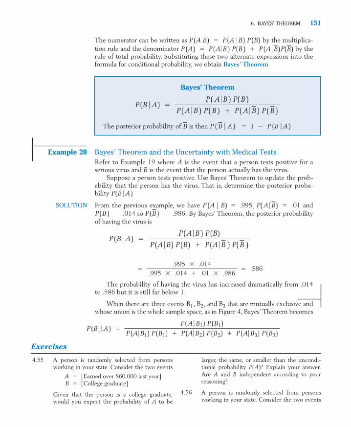
The numerator can be written as by the multiplica-tion rule and the denominator by therule of total probability. Substituting these two alternate expressions into theformula for conditional probability, we obtain Bayes’ Theorem.
P(B)P (A) � P(A� B) P(B) � P(A � B)P(A B) � P(A � B) P(B)
6. BAYES’ THEOREM 151
Bayes’ Theorem
The posterior probability of is then P ( B � A ) � 1 � P (B � A )B
P(B � A) �P( A � B ) P( B )
P( A � B ) P( B ) � P( A � B ) P( B )
Example 20 Bayes’ Theorem and the Uncertainty with Medical TestsRefer to Example 19 where A is the event that a person tests positive for aserious virus and B is the event that the person actually has the virus.
Suppose a person tests positive. Use Bayes’ Theorem to update the prob-ability that the person has the virus. That is, determine the posterior proba-bility
SOLUTION From the previous example, we have . andso By Bayes’ Theorem, the posterior probability
of having the virus is
The probability of having the virus has increased dramatically from .014to .586 but it is still far below 1.
When there are three events B1, B2, and B3 that are mutually exclusive andwhose union is the whole sample space, as in Figure 4, Bayes’ Theorem becomes
P(B1� A) �P(A � B1) P(B1)
P(A� B1) P(B1) � P(A� B2) P(B2) � P(A� B3) P(B3)
�.995 � .014
.995 � .014 � .01 � .986� .586
P(B � A) �P(A � B ) P(B)
P(A � B) P(B) � P(A � B ) P( B )
P(B) � .986.P(B) � .014P(A � B) � .01P (A � B) � .995
P(B � A)
4.55 A person is randomly selected from personsworking in your state. Consider the two events
[Earned over $60,000 last year][College graduate]
Given that the person is a college graduate,would you expect the probability of A to be
B �A �
larger, the same, or smaller than the uncondi-tional probability P(A)? Explain your answer.Are A and B independent according to yourreasoning?
4.56 A person is randomly selected from personsworking in your state. Consider the two events
Exercises
c04a.qxd 10/15/09 11:02 AM Page 151

[Lawyer][Driving a new luxury car]
Given that the person selected drives a newluxury car, would you expect the probability ofA to be larger, the same, or smaller than theunconditional probability P(A)? Explain youranswer. Are A and B independent according toyour reasoning?
4.57 Refer to Exercise 4.43. Find
(a) the conditional probability that B occursgiven that A occurs.
(b) The conditional probability that B doesnot occur given that A occurs.
(c) The conditional probability that B occursgiven that A does not occur.
4.58 Refer to Exercise 4.45. Find
(a) the conditional probability that A occursgiven that B occurs.
(b) the conditional probability that B occursgiven that A does not occur.
4.59 The following data relate to the proportions ina population of drivers.
The probabilities are given in the accompany-ing Venn diagram. Find P(B �A). Are A and Bindependent?
4.60 Suppose and
(a) Determine all the probabilities needed tofill in the accompanying table.
P (AB) � .20.P(B) � .32,P(A) � .55,
B � Accident in current year A � Defensive driver training last year
B �A �
152 CHAPTER 4/PROBABILITY
(b) Find the conditional probability of Agiven that B does not occur.
4.61 For two events A and B, the following proba-bilities are given.
P(A) � .4 P (B) � .25 P(A � B) � .7
Use the appropriate laws of probability to cal-culate
(a)
(b)
(c)
4.62 Records of student patients at a dentist’s officeconcerning fear of visiting the dentist suggestthe following proportions.
For a student selected at random, consider theevents
(a) Find the probabilities
(b) Are A and M independent?
4.63 An urn contains two green balls and threered balls. Suppose two balls will be drawn atrandom one after another and without re-placement (i.e., the first ball drawn is not re-turned to the urn before the second one isdrawn).
(a) Find the probabilities of the events
(b) Are the two events independent? Why orwhy not?
B � [Green ball appears in the second draw]
A � [Green ball appears in the first draw]
P(M) P(A � M)
P(A) P(AM)
A � [Fear] M � [Middle school]
P(A � B)
P(AB)
P(A)
A
.1 .05
.849
.00
1
B
B
A .55.20
.32
A
B
School
Elementary Middle High
Fear .12 .08 .05Do not fear .28 .25 .22
c04a.qxd 10/15/09 11:02 AM Page 152

4.64 Refer to Exercise 4.63. Now suppose twoballs will be drawn with replacement (i.e., thefirst ball drawn will be returned to the urnbefore the second draw). Repeat parts (a)and (b).
4.65 In a county, men constitute 60% of the laborforce. The rates of unemployment are 5.1%and 4.3% among males and females, respec-tively.
(a) In the context of selecting a worker atrandom from the country labor force,state what probabilities the foregoing per-centages represent. (Use symbols such asM for male, E for employed.)
(b) What is the overall rate of unemploymentin the county?
(c) If a worker selected at random is found tobe unemployed, what is the probabilitythat the worker is a woman?
4.66 If the probability of running out of gas is .03and the probability the electronic starting sys-tem will not work is .01,
(a) what is the probability that there will beenough gas and that the starting systemwill work? Assume the two events are in-dependent.
(b) When may independence be a poor as-sumption?
4.67 Suppose and
(a) Determine if A and B are in-dependent.
(b) Determine if A and B aremutually exclusive.
(c) Find if A and B are mutually ex-clusive.
4.68 Refer to Exercise 4.49.
(a) If a fast food restaurant selected at ran-dom is found to comply with safety stan-dards, what is the probability that it vio-lates sanitary standards?
(b) If a restaurant selected at random is foundto violate at least one of the two stan-dards, what is the probability that it com-plies with safety standards?
P(A� B)
P(A � B)
P(A � B)
P(B) � .22.P(A) � .6
6. BAYES’ THEOREM 153
4.69 In a shipment of 12 room air conditioners, thereare 3 with defective thermostats. Two air condi-tioners will be selected at random and inspectedone after another. Find the probability that:
(a) The first is defective.
(b) The first is defective and the second good.
(c) Both are defective.
(d) The second air conditioner is defective.
(e) Exactly one is defective.
4.70 Refer to Exercise 4.69. Now suppose 3 air con-ditioners will be selected at random andchecked one after another. Find the probabilitythat:
(a) All 3 are good.
(b) The first 2 are good and the third defec-tive.
(c) Two are good and 1 defective.
4.71 Of 20 rats in a cage, 12 are males and 9 are in-fected with a virus that causes hemorrhagicfever. Of the 12 male rats, 7 are infected withthe virus. One rat is randomly selected fromthe cage.
(a) If the selected rat is found to be infected,what is the probability that it is a female?
(b) If the selected rat is found to be a male,what is the probability that it is infected?
(c) Are the events “the selected rat is in-fected” and “the selected rat is male” inde-pendent? Why or why not?
4.72 A restaurant critic goes to a place twice. If shehas an unsatisfactory experience during bothvisits, she will go once more. Otherwise shewill make only the two visits.Assuming that the results for different visitsare independent and that the probability of asatisfactory experience in any one visit is .8
(a) assign probabilities to each outcome.
(b) Find the probability of at least two unsat-isfactory visits.
(c) Find the conditional probability of at leastone satisfactory visit given at least oneunsatisfactory visit.
c04a.qxd 10/15/09 11:02 AM Page 153

4.73 Of three events, A, B, and C, suppose events Aand B are independent and events B and C aremutually exclusive. Their probabilities are
.7, and Express the following events in set notationand calculate their probabilities.
(a) Both B and C occur.
(b) At least one of A and B occurs.
(c) B does not occur.
(d) All three events occur.
4.74 Approximately 40% of the Wisconsin popula-tion have type O blood. If 4 persons are se-lected at random to be donors, find P[at leastone type O].
4.75 The primary cooling unit in a nuclear powerplant has reliability .999. There is also a back-up cooling unit to substitute for the primaryunit when it fails. The reliability of the back-up unit is .910. Find the reliability of thecooling system of the power plant. Assumeindependence.
4.76 An accountant screens large batches of bills ac-cording to the following sampling inspectionplan. She inspects 4 bills chosen at randomfrom each batch and passes the batch if, amongthe 4, none is irregular. Find the probabilitythat a batch will be passed if, in fact:
(a) 5% of its bills are irregular.
(b) 20% of its bills are irregular.
4.77 An electronic scanner is successful in detectingflaws in a material in 80% of the cases. Threematerial specimens containing flaws will betested with the scanner. Assume that the testsare independent.
(a) List the sample space and assign probabil-ities to the simple events.
(b) Find the probability that the scanner issuccessful in at least two of the three cases.
4.78 Refer to Exercise 4.52. Given that a landfillselected at random is found to have a high
P(C) � .3.P(B) � .2,P(A) �
154 CHAPTER 4/PROBABILITY
concentration of mercury, what is the proba-bility that its concentration is:
(a) High in barium?
(b) Low in both arsenic and barium?
(c) High in either arsenic or barium?
4.79 Of the patients reporting to a clinic with thesymptoms of sore throat and fever, 25% havestrep throat, 40% have an allergy, and 10%have both.
(a) What is the probability that a patient se-lected at random has strep throat, an al-lergy, or both?
(b) Are the events “strep throat” and “allergy”independent?
*4.80 Consider tossing two fair coins and the events
A: Head in the first toss
B: Head in the second toss
C: Both heads or both tails in the twotosses
(a) Verify that the property of independenceholds for all event pairs.
(b) Show that is different from theproduct (This illus-trates the fact that pairwise independencedoes not ensure complete independence.)
4.81 Imperfect clinical test. Repeat Example 20but change to .96.
4.82 Carol and Karl both solve difficult computerproblems that come to the student desk. Carolmakes 60% of the repairs and Karl 40%. How-ever, Carol’s repairs are incomplete 4% of thetime and Karl’s are incomplete 6% of thetime.
(a) Determine the probability that a repair isincomplete.
(b) If a repair is found to be incomplete,what is the probability that the repair wasmade by Karl?
P(A � B)
P(A)P(B)P(C).P(ABC)
c04a.qxd 10/15/09 11:02 AM Page 154

7. RANDOM SAMPLING FROM A FINITE POPULATION
In our earlier examples of probability calculations, we have used the phrase“randomly selected” to mean that all possible selections are equally likely. It usu-ally is not difficult to enumerate all the elementary outcomes when both thepopulation size and sample size are small numbers. With larger numbers, mak-ing a list of all the possible choices becomes a tedious job. However, a countingrule is available that enables us to solve many probability problems.
We begin with an example where the population size and the sample sizeare both small numbers so all possible samples can be conveniently listed.
Example 21 Selecting a Random Sample of Size 2 from a Population of Size 5There are five qualified applicants for two editorial positions on a collegenewspaper. Two of these applicants are men and three women. If the posi-tions are filled by randomly selecting two of the five applicants, what is theprobability that neither of the men is selected?
SOLUTION Suppose the three women applicants are identified as a, b, and c and the twomen as d and e. Two members are selected at random from the population:
{a, b, c, d, e}
women men
The possible samples may be listed as
{a, b} {b, c } {c, d } {d, e}{a, c } {b,d } {c, e }{a, d} {b, e }{a, e}
As the list shows, our sample space has 10 elementary outcomes. The notionof random selection entails that these are all equally likely, so each is assignedthe probability Let A represent the event that two women are selected.Scanning our list, we see that A consists of the three elementary outcomes
{a, b} {a, c} {b, c}Consequently,
Note that our probability calculation in Example 21 only requires knowl-edge of the two counts: the number of elements in S and the number of ele-ments in A. Can we arrive at these counts without formally listing the samplespace? An important counting rule comes to our aid. (See Appendix A.2)
P(A) �No. of elements in ANo. of elements in S
�310
� .3
110 .
7. RANDOM SAMPLING FROM A FINITE POPULATION 155
��
c04a.qxd 10/15/09 11:02 AM Page 155

More specifically, the numerator of the formula is the product of r
consecutive integers starting with N and proceeding downward. The denomina-tor is also the product of r consecutive integers, but starting with r and proceed-ing down to 1.
To motivate the formula, let us consider the number of possible choices (orcollections) of three letters from the seven letters {a, b, c, d, e, f, g }. This count is
denoted by .
It is easier to arrive at a formula for the number of ordered selections.The first choice can be any of the 7 letters, the second can be any of the re-maining 6, and the third can be any of the remaining 5. Thinking in terms ofa tree diagram (without actually drawing one), we arrive at the following count.
The number of ordered selections of 3 letters from 7 is given by theproduct 7 � 6 � 5.
Next, note that a particular collection, say {a, b, c}, can produce 3 � 2 � 1
orderings, as one can also verify by a tree diagram. The number of collec-
tions, each producing 3 � 2 � 1 orderings, generate a total of � 3 �
2 � 1 orderings. Because this count must equal 7 � 6 � 5, we get
This explains the formula of for the case N � 7 and r � 3.
Although not immediately apparent, there is a certain symmetry in the
counts The process of selecting r objects is the same as choosing N � r�Nr � .
�Nr �
�73� �
7 � 6 � 53 � 2 � 1
�73�
�73�
�73�
�Nr �
156 CHAPTER 4/PROBABILITY
The Rule of Combinations
Notation: The number of possible choices of r objects from a group of N
distinct objects is denoted by which reads as “N choose r.”
Formula:
�Nr � �
N � (N � 1) � ��� � (N � r � 1)r � (r � 1) � ��� � 2 � 1
�Nr � ,
c04a.qxd 10/15/09 11:02 AM Page 156

objects to leave behind. Because every choice of r objects corresponds to achoice of objects,
This relation often simplifies calculations. Since we take
Example 22 Evaluating Some Combinations
Calculate the values of and
SOLUTION
Using the relation we have
Example 23 Calculating a Probability Using CombinationsRefer to Example 21 concerning a random selection of two persons from agroup of two men and three women. Calculate the required probability with-out listing the sample space.
SOLUTION The number of ways two persons can be selected out of five is given by
Random selection means that the 10 outcomes are equally likely. Next, weare to count the outcomes that are favorable to the event A that both se-lected persons are women. Two women can be selected out of three in
Taking the ratio, we obtain the result
P (A) �3
10� .3
�32� �
3 � 22 � 1
� 3 ways
�52� �
5 � 42 � 1
� 10
�1511� � �15
4 � � 1365
�Nr � � � N
N � r� ,
�154 � �
15 � 14 � 13 � 124 � 3 � 2 � 1
� 1365�52� �
5 � 42 � 1
� 10
�1511� .�15
4 � ,�52� ,
�N0� � 1.�N
N� � 1,
choose leaver N � r
N� � N
N � r��Nr �
N � r
7. RANDOM SAMPLING FROM A FINITE POPULATION 157
c04a.qxd 10/15/09 11:02 AM Page 157

Example 24 Probabilities of Being Selected under Random SelectionAfter some initial challenges, there remain 16 potential jurors of which 10are male and 6 female. The defense attorney can dismiss 4 additional personson the basis of answers to her questions.
(a) How many ways can the 4 additional jurors be selected for dismissal?
(b) How many selections are possible that result in 1 male and 3 fe-males being dismissed?
(c) If the selection process were random, what is the probability that 1male and 3 females would be dismissed?
SOLUTION(a) According to the counting rule the number of ways 4 jurors
can be selected out of 16 is
(b) One male can be chosen from 10 in ways. Also, 3 fe-
males can be chosen from 6 in
Each of the 10 choices of a male can accompany each of the 20choices of 3 females. Reasoning from the tree diagram, we con-clude that the number of possible samples with the stated compo-sition is
(c) Random sampling requires that the 1820 possible samples are allequally likely. Of these, 200 are favorable to the event A � [1 maleand 3 females]. Consequently,
The notion of a random sample from a finite population is crucial to statisti-cal inference. In order to generalize from a sample to the population, it is imper-ative that the sampling process be impartial. This criterion is evidently met if weallow the selection process to be such that all possible samples are given equalopportunity to be selected. This is precisely the idea behind the term randomsampling, and a formal definition can be phrased as follows.
P (A) �200
1820� .110
�101 � � �6
3� � 10 � 20 � 200
�63� �
6 � 5 � 43 � 2 � 1
� 20 ways
�101 � � 10
�164 � �
16 � 15 � 14 � 134 � 3 � 2 � 1
� 1820
�Nr � ,
158 CHAPTER 4/PROBABILITY
c04a.qxd 10/15/09 11:02 AM Page 158

Note that this is a conceptual rather than an operational definition of a ran-dom sample. On the surface, it might seem that a haphazard selection by theexperimenter would result in a random sample. Unfortunately, a seemingly hap-hazard selection may have hidden bias. For instance, when asked to name a ran-dom integer between 1 and 9, more persons respond with 7 than any othernumber. Also, odd numbers are more popular than even numbers. Therefore, theselection of objects must be entrusted to some device that cannot think; inother words, some sort of mechanization of the selection process is needed tomake it truly haphazard!
To accomplish the goal of a random selection, one may make a card for eachof the N members of the population, shuffle, and then draw n cards. Thismethod is easy to understand but awkward to apply to large-size populations. Itis best to use random numbers as described in Chapter 1. Random numbers areconveniently generated on a computer (see Chapter 4 Technology section).
At the beginning of this chapter, we stated that probability constitutes themajor vehicle of statistical inference. In the context of random sampling from apopulation, the tools of probability enable us to gauge the likelihood of variouspotential outcomes of the sampling process. Ingrained in our probability calcula-tions lies the artificial assumption that the composition of the population isknown. The route of statistical inference is exactly in the opposite direction, asdepicted in Figure 5. It is the composition of the population that is unknown
7. RANDOM SAMPLING FROM A FINITE POPULATION 159
A sample of size n selected from a population of N distinct objects is saidto be a random sample if each collection of size n has the same probability
of being selected.1 /�Nn�
?
?
A probability problem asks:
“What is the probability thatthe sample will have …?
Statistical inference asks:
“What models of the population(blackbox) make the observedsample plausible?
Figure 5 Probability versus statistical inference.
c04a.qxd 10/15/09 11:02 AM Page 159

while we have at hand the observations (data) resulting from a random sample.Our object of inference is to ascertain what compositions (or models) of thepopulation are compatible with the observed sample data. We view a model asplausible unless probability calculations based on this model make the sampleoutcome seem unlikely.
Exercises
160 CHAPTER 4/PROBABILITY
4.83 Evaluate:
(a) (b) (c)
(d) (e) (f)
4.84 List all the samples from {a, b, c, d, e} when (a)2 out of 5 are selected, (b) 3 out of 5 are se-lected. Count the number of samples in eachcase.
4.85 Of 10 available candidates for membership ina university committee, 6 are men and 4 arewomen. The committee is to consist of 4 per-sons.
(a) How many different selections of thecommittee are possible?
(b) How many selections are possible if thecommittee must have 2 men and 2women?
4.86 If a coin is tossed 11 times, the outcome can berecorded as an 11-character sequence of H’s andT’s according to the results of the successivetosses. In how many ways can there be 4 H’sand 7 T’s? (Put differently, in how many wayscan one choose 4 positions out of 11 to put theletter H?)
4.87 A psychologist will select 5 preschool childrenfrom a class of 11 students in order to try outnew abuse awareness material.
(a) How many different selections are possi-ble?
(b) Suppose 4 of the 11 children are males. Ifthe 5 selected children were to consist of2 males and 3 females, how many differ-ent selections are possible?
�3027��30
3 ��2220�
�222 ��10
4 ��63�
4.88 Out of 12 people applying for an assembly job,3 cannot do the work. Suppose two personswill be hired.
(a) How many distinct pairs are possible?
(b) In how many of the pairs will 0 or 1 per-son not be able to do the work?
(c) If two persons are chosen in a randommanner, what is the probability that nei-ther will be able to do the job?
4.89 After a preliminary screening, the list of quali-fied jurors consists of 10 males and 7 females.The 5 jurors the judge selects from this list areall males. Did the selection process seem todiscriminate against females? Answer this bycomputing the probability of having no femalemembers in the jury if the selection is random.
4.90 Suppose you participate in a lottery conductedby a local store to give away four prizes. Eachcustomer is allowed to place 2 cards in the bar-rel. Suppose the barrel contains 5000 cardsfrom which the 4 winning cards will be chosenat random. What is the probability that at leastone of your cards will be drawn?
4.91 A batch of 20 used automobile alternators con-tains 4 defectives. If 3 alternators are sampled atrandom, find the probability of the event
(a) A � [None of the defectives appear]
(b) B � [Exactly two defectives appear]
4.92 Ordered sampling versus unordered sam-pling. Refer to Exercise 4.91. Suppose thesampling of 3 alternators is done by randomlychoosing one after another and without re-placement. The event A can then be describedas G1G2G3 , where G denotes “good” and thesuffixes refer to the order of the draws. Use the
c04a.qxd 10/15/09 11:02 AM Page 160

method of Example 14 to calculate P(A) andP(B ). Verify that you get the same results as inExercise 4.91.
This illustrates the following fact: To arriveat a random sample, we may randomly drawone object at a time without replacement andthen disregard the order of the draws.
4.93 A college senior is selected at random fromeach state. Next, one senior is selected at ran-dom from the group of 50. Does this proce-dure produce a senior selected at random fromthose in the United States?
4.94 An instructor will choose 3 problems from aset of 7 containing 3 hard and 4 easy problems.If the selection is made at random, what is theprobability that only the hard problems arechosen?
4.95 Nine agricultural plots for an experiment arelaid out in a square grid as shown. Three plotsare to be selected at random.
(a) Find the probability that all3 are in the same row.
(b) Find the probability that all3 are in different rows.
4.96 In one area of an orchard, there are 17 trees, ofwhich 10 are bushy and 7 lean. If 4 trees arerandomly selected for testing a new spray,what is the probability that exactly 2 bushytrees are selected?
*4.97 Referring to Exercise 4.96, now suppose thatthe trees are located in two rows: Row A has 8trees of which 4 are bushy, and row B has 9trees of which 6 are bushy. Two trees are to berandomly selected from each row for testingthe spray, and the selections are independentfor the two rows.
(a) Find the probability that the trees selectedin row A are both bushy and those se-lected in row B are both lean.
(b) Find the probability that of the total of 4trees selected in the manner describedabove, exactly 2 are bushy.
4.98 Are the following methods of selection likelyto produce a random sample of 5 studentsfrom your school? Explain.
7. RANDOM SAMPLING FROM A FINITE POPULATION 161
(a) Pick 5 students throwing flying discs onthe mall.
(b) Pick 5 students who are studying in the li-brary on Friday night.
(c) Select 5 students sitting near you in yourstatistics course.
4.99 An advertisement seeking volunteers for a clini-cal research draws 11 respondents. Of these re-spondents, 5 are below age 30 and 6 are over30. The researcher will randomly select 4 per-sons to assign to a particular treatment regimen.
(a) How many selections are possible?
(b) What is the probability exactly 3 of the se-lected persons are below age 30?
*4.100 Refer to Exercise 4.99, and further suppose thatthe 5 respondents who are below 30 consist of2 males and 3 females, whereas those above 30consist of 4 males and 2 females. Now, the re-searcher wants to randomly select 2 males and 2females to be assigned to the treatment regi-men. (The random selections from the differentsexes are, of course, independent.)
(a) How many selections are possible?
(b) What is the probability that both selectedmales are over 30 and both selected fe-males are under 30?
4.101 A box of tulip bulbs contains six bulbs thatproduce yellow flowers and five bulbs thatproduce red flowers. Four bulbs are to be ran-domly selected without replacement. Find theprobability that:
(a) Exactly two of the selected bulbs producered flowers.
(b) At least two of the selected bulbs producered flowers.
(c) All four selected bulbs produce flowers ofan identical color.
4.102 A file cabinet has eight student foldersarranged alphabetically according to last name.Three files are selected at random.
(a) How many different selections are possible?
(b) Find the probability that the selected fold-ers are all adjacent.
(Hint: Enumerate the selections of adja-cent folders.)
1 2 3
4 5 6
7 8 9
c04a.qxd 10/15/09 11:02 AM Page 161
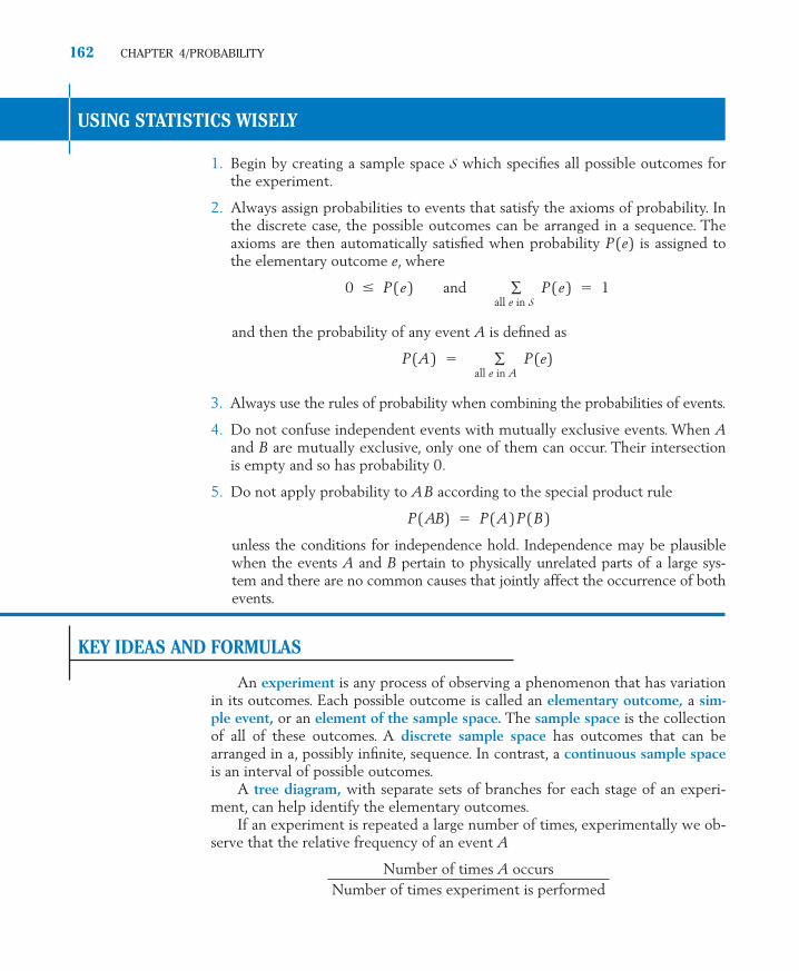
USING STATISTICS WISELY
1. Begin by creating a sample space S which specifies all possible outcomes forthe experiment.
2. Always assign probabilities to events that satisfy the axioms of probability. Inthe discrete case, the possible outcomes can be arranged in a sequence. Theaxioms are then automatically satisfied when probability P(e) is assigned tothe elementary outcome e, where
0 � P(e) and ∑ P(e) � 1all e in S
and then the probability of any event A is defined as
P(A) � ∑ P(e)all e in A
3. Always use the rules of probability when combining the probabilities of events.
4. Do not confuse independent events with mutually exclusive events. When Aand B are mutually exclusive, only one of them can occur. Their intersectionis empty and so has probability 0.
5. Do not apply probability to AB according to the special product rule
P(AB) � P(A)P(B)
unless the conditions for independence hold. Independence may be plausiblewhen the events A and B pertain to physically unrelated parts of a large sys-tem and there are no common causes that jointly affect the occurrence of bothevents.
KEY IDEAS AND FORMULAS
An experiment is any process of observing a phenomenon that has variationin its outcomes. Each possible outcome is called an elementary outcome, a sim-ple event, or an element of the sample space. The sample space is the collectionof all of these outcomes. A discrete sample space has outcomes that can bearranged in a, possibly infinite, sequence. In contrast, a continuous sample spaceis an interval of possible outcomes.
A tree diagram, with separate sets of branches for each stage of an experi-ment, can help identify the elementary outcomes.
If an experiment is repeated a large number of times, experimentally we ob-serve that the relative frequency of an event A
Number of times A occursNumber of times experiment is performed
162 CHAPTER 4/PROBABILITY
c04b.qxd 10/15/09 11:00 AM Page 162

will stabilize at a numerical value. This long-run stability of relative frequencymotivates us to assign a number P (A) between 0 and 1 as the probability of theevent A. In the other direction, we can approximate the probability of anyevent by repeating an experiment many times.
When the sample space is discrete, probability is then expressed as any as-signment of non-negative numbers to the elementary outcomes so that proba-bility 1 is assigned to the whole sample space. The probability model of an ex-periment is described by:
1. The sample space, a list or statement of all possible distinct outcomes.2. Assignment of probabilities to all the elementary outcomes.
and where the sum extends over all e in S.
The probability of an event A is the sum of the probabilities of all the ele-mentary outcomes that are in A.
P (A) � ∑ P (e )all e in A
A uniform probability model holds when all the elementary outcomes in Sare equiprobable. With a uniform probability model,
In all cases, P (A), viewed as the long-run relative frequency of A, can be ap-proximately determined by repeating the experiment a large number of times.
Elementary outcomes and events can be portrayed in a Venn diagram. Theevent operations union, intersection, and complement can be depicted as wellas the result of combining several operations.
The three basic laws of probability are
Law of complement
Addition law
Multiplication law
These are useful in probability calculations when events are formed withthe operations of complement, union, and intersection.
Two events are incompatible or mutually exclusive if their intersection isempty. In that case we have the special addition law for incompatible events
The concept of conditional probability is useful to determine how the prob-ability of an event A must be revised when another event B has occurred. Itforms the basis of the multiplication law of probability and the notion of inde-pendence of events.
Conditional probability of A given B
P(A � B) �P(AB)P(B )
P( A � B ) � P ( A ) � P ( B )
P ( AB ) � ( B ) P (A � B )
P ( A � B ) � P( A ) � P ( B ) � P ( AB )
P ( A ) � 1 � P ( A )
P ( A ) �No. of e in ANo. of e in S
� P ( e ) � 1,P ( e ) � 0
KEY IDEAS AND FORMULAS 163
c04b.qxd 10/15/09 11:00 AM Page 163
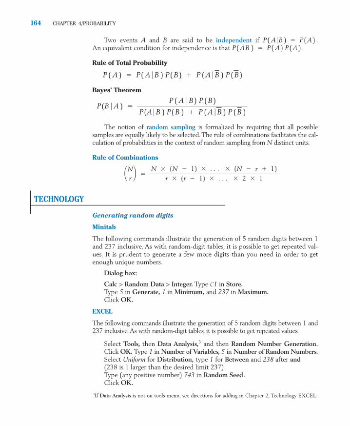
Two events A and B are said to be independent if .An equivalent condition for independence is that .
Rule of Total Probability
Bayes’ Theorem
The notion of random sampling is formalized by requiring that all possiblesamples are equally likely to be selected.The rule of combinations facilitates the cal-culation of probabilities in the context of random sampling from N distinct units.
Rule of Combinations
TECHNOLOGY
Generating random digits
Minitab
The following commands illustrate the generation of 5 random digits between 1and 237 inclusive. As with random-digit tables, it is possible to get repeated val-ues. It is prudent to generate a few more digits than you need in order to getenough unique numbers.
Dialog box:
Calc > Random Data > Integer. Type C1 in Store.Type 5 in Generate, 1 in Minimum, and 237 in Maximum.Click OK.
EXCEL
The following commands illustrate the generation of 5 random digits between 1 and237 inclusive.As with random-digit tables, it is possible to get repeated values.
Select Tools, then Data Analysis,3 and then Random Number Generation.Click OK. Type 1 in Number of Variables, 5 in Number of Random Numbers.Select Uniform for Distribution, type 1 for Between and 238 after and (238 is 1 larger than the desired limit 237)Type (any positive number) 743 in Random Seed.Click OK.
�Nr � �
N � (N � 1) � . . . � (N � r � 1)r � (r � 1) � . . . � 2 � 1
P (B � A ) �P ( A � B ) P ( B )
P (A � B ) P ( B ) � P ( A � B ) P ( B )
P ( A ) � P ( A � B ) P ( B ) � P ( A � B ) P ( B )
P ( A B ) � P ( A ) P ( A )P ( A �B ) � P ( A )
164 CHAPTER 4/PROBABILITY
3If Data Analysis is not on tools menu, see directions for adding in Chapter 2, Technology EXCEL.
c04b.qxd 10/15/09 11:00 AM Page 164

The random numbers appear in the first column of the spreadsheet. Youjust ignore the decimal part of each entry to obtain random digits between 1and 237 inclusive.
TI-84/83 PLUS
The following commands show the generation of 5 random digits between 1 and237 inclusive. As with random-digit tables, it is possible to get repeated values.
Enter any nonzero number on the Home screen.Press the STO button. Press the MATH button.Select the PRB menu and then select 1: rand.From the Home screen press ENTER.Press the MATH button. Select the PRB menu and then 5: randInt(.With randInt( on the Home screen, enter 1 and 237 so that the following appearsrandInt (1,237, 5)Press ENTER to obtain the 5 random digits.
8. REVIEW EXERCISES
:
8. REVIEW EXERCISES 165
4.103 Describe the sample space for each of the fol-lowing experiments.
(a) The number of different words used in asentence containing 24 words.
(b) The air pressure (psi) in the right fronttire of a car.
(c) In a survey, 50 students are asked torespond “yes” or “no” to the question“Do you hold at least a part-timejob while attending school?” Only thenumber answering “yes” will berecorded.
(d) The time a TV satellite remains in opera-tion.
4.104 For the experiments in Exercise 4.103, whichsample spaces are discrete and which are con-tinuous?
4.105 Identify these events in the correspondingparts of Exercise 4.103.
(a) More than 22 words.
(b) Air pressure less than or equal to 28 psi.
(c) At most 25% hold jobs.
(d) Less than 500.5 days.
4.106 Examine each of these probability assignmentsand state what makes it improper.
(a) Concerning tomorrow’s weather,
P(Rain) � .4P(Cloudy but no rain) � .4P(Sunny) � .3
(b) Concerning your passing of the statisticscourse,
P(Pass) � 1.1 P(Fail) � .1
(c) Concerning your grades in statistics andeconomics courses,
P(A in statistics) � .3P(A in economics) � .7P(A’s in both statistics and economics) � .4
4.107 A driver is stopped for erratic driving, and thealcohol content of his blood is checked. Spec-ify the sample space and the event A �[level exceeds legal limit] if the legal limitis .10%.
4.108 The Wimbledon men’s tennis championshipends when one player wins three sets.
(a) How many elementary outcomes end inthree sets? In four?
*(b) If the players are evenly matched, what isthe probability that the tennis matchends in four sets?
c04b.qxd 10/15/09 11:00 AM Page 165

4.109 There are four tickets numbered 1, 2, 3, and 4.Suppose a two-digit number will be formed byfirst drawing one ticket at random and thendrawing a second ticket at random from the re-maining three. (For instance, if the first ticketdrawn shows 3 and the second shows 1, thenumber recorded is 31.) List the sample spaceand determine the following probabilities.
(a) An even number.
(b) A number larger than 20.
(c) A number between 22 and 30.
4.110 To compare two varieties of wheat, say, a andb, a field trial will be conducted on four squareplots located in two rows and two columns.Each variety will be planted on two of theseplots.
166 CHAPTER 4/PROBABILITY
4.113 A letter is chosen at random from the word“VOLUNTEER.”
(a) What is the probability that it is a vowel?
(b) What is the probability that it is a T or V?
4.114 Does the uniform model apply to the follow-ing observations? Explain.
(a) Day of week on which the most personsdepart by airplane from Chicago.
(b) Day of week on which the monthly lowtemperature occurs.
(c) Day of week on which the maximumamount of ozone is recorded.
(d) Month of year when a department storehas the maximum sales revenues.
4.115 A three-digit number is formed by arrangingthe digits 1, 2, and 5 in a random order.
(a) List the sample space.
(b) Find the probability of getting a numberless than 400.
(c) What is the probability that an evennumber is obtained?
4.116 A late shopper for Valentine’s flowers calls byphone to have a flower wrapped. The store hasonly 5 roses, of which 3 will open by the nextday, and 6 tulips, of which 2 will open by thenext day.
(a) Construct a Venn diagram and show theevents A � [Rose], and B � [Willopen next day].
(b) If the store selects one flower at random,find the probability that it will not openby the next day.
4.117 In checking the conditions of a used car, let Adenote the event that the car has a faultytransmission, B the event that it has faultybrakes, and C the event that it has a faulty ex-haust system. Describe in words what the fol-lowing events represent:
(a) (b) ABC
(c) (d)
4.118 Express the following statements in the nota-tions of the event operations.
A � BA B C
A � B
(a) List all possible assignments for variety a.
(b) If the assignments are made completely atrandom, find the probability that theplots receiving variety a are:
(i) In the same column.
(ii) In different rows and differentcolumns.
4.111 Refer to Exercise 4.110. Instead of a com-pletely random choice, suppose a plot is cho-sen at random from each row and assigned tovariety a. Find the probability that the plotsreceiving a are in the same column.
4.112 Chevalier de Méré, a French nobleman of theseventeenth century, reasoned that in a singlethrow of a fair die, P(1) � so in two throws,P(1 appears at least once) �What is wrong with the above reasoning? Usethe sample space of Exercise 4.21 to obtainthe correct answer.
16 � 1
6 � 13 .
16 ,
1
3
Plot arrangement
4
2
c04b.qxd 10/15/09 11:01 AM Page 166

(a) A occurs and B does not.
(b) Neither A nor B occurs.
(c) Exactly one of the events A and B occurs.
4.119 Suppose each of the numbers .1, .3, and .5represents the probability of one of the eventsA, AB, and Connect the probabilitiesto the appropriate events.
4.120 From the probabilities exhibited in this Venndiagram, find and
4.121 Using event relations, express the followingevents in terms of the three events A, B, and C.
(a) All three events occur.
(b) At least one of the three events occurs.
(c) A and B occur and C does not.
(d) Only B occurs.
4.122 Concerning three events A, B, and C, theprobabilities of the various intersections aregiven in the accompanying table. [For instance,
]
(a) Draw a Venn diagram, identify the inter-sections, and mark the probabilities.
P ( ABC ) � .10.
P ( BC ).P ( B � C ),P ( AB ),P ( A ),
A � B.
8. REVIEW EXERCISES 167
(b) Determine the probabilities
P(AB) P(C )
(c) Fill in the accompanying probability tableconcerning the events A and B.
4.123 Referring to Exercise 4.122, calculate theprobabilities of the following events.
(a) Both B and C occur.
(b) Either B or C occurs.
(c) B occurs and C does not occur.
(d) Only one of the three events A, B, and Coccurs.
4.124 Concerning three events A, B, and C, the fol-lowing probabilities are specified.
P(A) � .51 P(AB ) � .17 P(ABC ) � .12P(B) � .45 P(BC ) � .20P(C) � .50 P(AC) � .33
Draw a Venn diagram and determine the prob-abilities of all the intersections that appear inthe diagram. Also, make a probability table likethe one given in Exercise 4.122.
4.125 Referring to Exercise 4.124, find the probabil-ity that:
(a) B occurs and C does not occur.
(b) At least one of the events A and B occurs.
(c) Exactly two of the events A, B, and C oc-cur.
4.126 Suppose a fair die has its even-numbered facespainted red and the odd-numbered faces arewhite. Consider the experiment of rolling thedie once and the events
B � [Red face shows up]A � [2 or 3 shows up]
P(AC )
A
.1 .18
.02
.4.3
B
C
B
C C
A .05 .10 .05 .17.20 .15 .18 .10A
CC
B
B
AA
B
c04b.qxd 10/15/09 11:01 AM Page 167

Find the following probabilities:
(a) P(A ) (b) P(B ) (c) P(AB )
(d) P(A �B ) (e)
4.127 Given and findP(A �B ). If, further, are A and Bindependent?
4.128 Suppose three events A, B, and C are such thatB and C are mutually exclusive and
(a) Show the events in a Venn diagram.
(b) Determine the probabilities of all the in-tersections and mark them in the Venndiagram.
(c) Find the probability that only one of thethree events occurs.
4.129 Refer to Exercise 4.128. For each pair ofevents given below, determine whether or notthe events are independent.
(a) A, C
(b)
4.130 Let A be the event that a person is a moderateor heavy drinker and B be the event that theperson is female. For a person selected at ran-dom in the United States, the probabilities are4
(a) Express in words, in the context of thisproblem, the third probability statement.
(b) Determine the probability that the personselected is a moderate or heavy drinker.
(c) If the person selected is found to be amoderate or heavy drinker, what is theprobability of being female?
4.131 Refer to the probability table given in Exercise4.122 concerning three events A, B, and C.
(a) Find the conditional probability of Agiven that B does not occur.
(b) Find the conditional probability of Bgiven that both A and C occur.
(c) Determine whether or not the events Aand C are independent.
P ( B ) � .50 P ( A � B ) � .12 P ( A � B ) � .29
AB, C
P(A � B) �23
P( AC ) � .1
P(C ) � .25P(B) � .3P(A) � .6
P(A) � .8,P(B) � .5,P( AB ) � .4
P ( A � B )
168 CHAPTER 4/PROBABILITY
4.132 Mr. Hope, a character apprehended by SherlockHolmes, was driven by revenge to commit twomurders. He presented two seemingly identicalpills, one containing a deadly poison, to an ad-versary who selected one while Mr. Hope tookthe other. The entire procedure was then to berepeated with the second victim. Mr. Hopefelt that Providence would protect him, butwhat is the probability of the success of hisendeavor?
4.133 A bowl contains 15 marbles, of which 10 arenumbered 1 and 5 are numbered 2. Two mar-bles are to be randomly drawn from the bowlone after another and without replacement,and a two-digit number will be recorded ac-cording to the results. (For instance, if the firstmarble drawn shows 2 and the second shows1, the number recorded is 21.)
(a) List the sample space and determine theprobability of each outcome.
(b) Find the probability of getting an evennumber.
(c) Find the probability that the number islarger than 15.
4.134 Three production lines contribute to the totalpool of a company’s product. Line 1 provides20% to the pool and 10% of its products aredefective; Line 2 provides 50% to the pool and5% of its products are defective; Line 3 con-tributes 30% to the pool and 6% of its prod-ucts are defective.
(a) What percent of the items in the pool aredefective?
(b) Suppose an item is randomly selected fromthe pool and found to be defective. What isthe probability that it came from Line 1?
4.135 In an optical sensory experiment, a subjectshows a fast response (F ), a delayed response(D), or no response at all (N). The experimentwill be performed on two subjects.
(a) Using a tree diagram, list the sample space.
(b) Suppose, for each subject,and the re-
sponses of different subjects are independent.P ( N ) � .3,P ( D ) � .3,
P ( F ) � .4,
4National Center for Health Statistics, Health Behavior ofAdults, United States (September 2006).
c04b.qxd 10/15/09 11:01 AM Page 168

(i) Assign probabilities to the elemen-tary outcomes.
(ii) Find the probability that at leastone of the subjects shows a fast re-sponse.
(iii) Find the probability that both of thesubjects respond.
4.136 Four upper level undergraduate students areavailable to serve on a committee.
Two students will be selected at random toserve on the committee. Let
A: The students selected are of the same gender.
B: The students selected are the same year inschool.
(a) Make a Venn diagram showing the out-comes and the two events.
(b) Find the probability of .
(c) Are A and B independent? Explain whyor why not.
(d) Find the probability of
4.137 A local moving company owns 11 trucks.Three are randomly selected for compliancewith emission standards and all are found to benoncompliant. The company argues that theseare the only three which do not meet the stan-dards. Calculate the probability that, if onlythree are noncompliant, all three would be inthe sample. Comment on the veracity of thecompany’s claim.
4.138 In all of William Shakespeare’s works, he used884,647 different words. Of these, 14,376 ap-peared only once and 4343 appeared twice. Ifone word is randomly selected from a list ofthese 884,647 different words:
(a) What is the probability that the selectedword appears only once?
AB.
A � B
8. REVIEW EXERCISES 169
(b) What is the probability that the selectedword appears exactly twice?
(c) What is the probability that the selectedword appears more than twice?
(d) Suppose that, instead of randomly select-ing a word from the list of differentwords, you randomly select a word from abook of Shakespeare’s complete works byselecting a page, line, and word numberfrom a random-digit table. Is the proba-bility of selecting a word that appears ex-actly once larger, smaller, or the same asyour answer to part (a)?
4.139 An IRS agent receives a batch of 18 tax returnsthat were flagged by computer for possible taxevasions. Suppose, unknown to the agent, 7 ofthese returns have illegal deductions and theother 11 are in good standing. If the agent ran-domly selects 4 of these returns for audit, whatis the probability that:
(a) None of the returns that contain illegaldeductions are selected?
(b) At least 2 have illegal deductions?
*4.140 Polya’s urn scheme. An urn contains 4 redand 6 green balls. One ball is drawn at randomand its color is observed. The ball is then re-turned to the urn, and 3 new balls of the samecolor are added to the urn. A second ball isthen randomly drawn from the urn that nowcontains 13 balls.
(a) List all outcomes of this experiment (usesymbols such as R1G2 to denote the out-come of the first ball red and the secondgreen).
(b) What is the probability that the first balldrawn is green?
(c) What is the conditional probability ofgetting a red ball in the second drawgiven that a green ball appears in thefirst?
(d) What is the (unconditional) probability ofgetting a green ball in the second draw?
*4.141 Birthdays. It is somewhat surprising to learnthe probability that 2 persons in a classshare the same birthday. As an approximation,
Student Gender Year in school
1 M Junior2 M Senior3 F Junior4 F Senior
c04b.qxd 10/15/09 11:01 AM Page 169
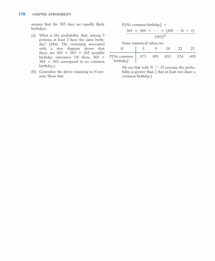
assume that the 365 days are equally likelybirthdays.
(a) What is the probability that, among 3persons, at least 2 have the same birth-day? (Hint: The reasoning associatedwith a tree diagram shows thatthere are 365 � 365 � 365 possiblebirthday outcomes. Of these, 365 �364 � 363 correspond to no commonbirthday.)
(b) Generalize the above reasoning to N per-sons. Show that
170 CHAPTER 4/PROBABILITY
N 5 9 18 22 23
P[No common .973 .905 .653 .524 .493birthday]
P[No common birthday] �
Some numerical values are
We see that with persons, the proba-bility is greater than that at least two share acommon birthday.)
12
N � 23
365 � 364 � � � � � (365 � N � 1)
(365)N
c04b.qxd 10/15/09 11:01 AM Page 170

1. Introduction2. Random Variables3. Probability Distribution
of a Discrete Random Variable4. Expectation (Mean) and Standard Deviation
of a Probability Distribution5. Successes and Failures—Bernoulli Trials6. The Binomial Distribution7. The Binomial Distribution in Context8. Review Exercises
5
Probability Distributions
c05.qxd 10/15/09 11:04 AM Page 171

Rescue Service on a LakeStudent sailors and other boaters on Lake Mendota are protected by a boatingrescue service. The relative frequencies from a long record for summer days leadto an approximate distribution of the number of rescues per day.
0 1
.1
.2
2 3 4 5 6
Number of rescues/day
Pro
babi
lity
The distribution describes the randomness of daily rescue activity. For instance, on anygiven day, the most probable number of rescues is 2. The distribution can be the basisfor decisions concerning manpower and the need for additional rescue boats.
© John Terrence Turner/FPG International/Getty Images
c05.qxd 10/15/09 11:04 AM Page 172

1. INTRODUCTION
A prescription for the probability model of an experiment contains two basicingredients: the sample space and the assignment of probability to each elemen-tary outcome. In Chapter 4, we encountered several examples where the ele-mentary outcomes had only qualitative descriptions rather than numerical val-ues. For instance, with two tosses of a coin, the outcomes HH, HT, TH, and TTare pairs of letters that identify the occurrences of heads or tails. If a new vac-cine is studied for the possible side effects of nausea, the response of each sub-ject may be severe, moderate, or no feeling of nausea. These are qualitative out-comes rather than measurements on a numerical scale.
Often, the outcomes of an experiment are numerical values: for example,the daily number of burglaries in a city, the hourly wages of students on summerjobs, and scores on a college placement examination. Even in the former situa-tion where the elementary outcomes are only qualitatively described, interestfrequently centers on some related numerical aspects. If a new vaccine is testedon 100 individuals, the information relevant for an evaluation of the vaccinemay be the numbers of responses in the categories—severe, moderate, or nonausea. The detailed record of 100 responses can be dispensed with once wehave extracted this summary. Likewise, for an opinion poll conducted on 500residents to determine support for a proposed city ordinance, the information ofparticular interest is how many residents are in favor of the ordinance, and howmany are opposed. In these examples, the individual observations are not nu-merical, yet a numerical summary of a collection of observations forms the nat-ural basis for drawing inferences. In this chapter, we concentrate on the numeri-cal aspects of experimental outcomes.
2. RANDOM VARIABLES
Focusing our attention on the numerical features of the outcomes, we introducethe idea of a random variable.
Corresponding to every elementary outcome of an experiment, a randomvariable assumes a numerical value, determined from some characteristic per-taining to the outcome. (In mathematical language, we say that a random vari-able X is a real-valued function defined on a sample space.) The word “random”serves as a reminder of the fact that, beforehand, we do not know the outcomeof an experiment or its associated value of X.
2. RANDOM VARIABLES 173
A random variable X associates a numerical value with each outcome ofan experiment.
c05.qxd 10/15/09 11:04 AM Page 173

Example 1 The Number of Heads as a Random VariableConsider X to be the number of heads obtained in three tosses of a coin. Listthe numerical values of X and the corresponding elementary outcomes.
SOLUTION First, X is a variable since the number of heads in three tosses of a coin canhave any of the values 0, 1, 2, or 3. Second, this variable is random in thesense that the value that would occur in a given instance cannot be predictedwith certainty. We can, though, make a list of the elementary outcomes andthe associated values of X.
Note that, for each elementary outcome there is only one value of X.However, several elementary outcomes may yield the same value. Scanningour list, we now identify the events (i.e., the collections of the elementaryoutcomes) that correspond to the distinct values of X.
Guided by this example, we observe the following general facts.
The events corresponding to the distinct values of X are incompatible.
The union of these events is the entire sample space.
Typically, the possible values of a random variable X can be determined di-rectly from the description of the random variable without listing the sample
174 CHAPTER 5/PROBABILITY DISTRIBUTIONS
Outcome Value of X
HHH 3HHT 2HTH 2HTT 1THH 2THT 1TTH 1TTT 0
Numerical Value Composition ofof X as an Event the Event
[ X � 0 ] � { TTT }[ X � 1 ] � { HTT, THT, TTH }[ X � 2 ] � {HHT, HTH,THH}[ X � 3 ] � { HHH }
c05.qxd 10/15/09 11:04 AM Page 174

space. However, to assign probabilities to these values, treated as events, it issometimes helpful to refer to the sample space.
Example 2 A Random Variable That Is a Count with a Finite Maximum ValueFifty cars are entered in a 100-mile road race. Let X be the number of carsthat actually finish the race. Here X could conceivably take any of the values0, 1, . . . , 50.
Example 3 A Random Variable That Is a Count with No Upper LimitOnce a week, a student buys a single lottery ticket. Let X be the number oftickets she purchases before she wins at least $1000 on a ticket. The possiblevalues of X are then 1, 2, 3, . . . , where the list never terminates.
A random variable is said to be discrete if it has either a finite number ofvalues or infinitely many values that can be arranged in a sequence. All the pre-ceding examples are of this type. On the other hand, if a random variable repre-sents some measurement on a continuous scale and is therefore capable of as-suming all values in an interval, it is called a continuous random variable. Ofcourse, any measuring device has a limited accuracy and, therefore, a continuousscale must be interpreted as an abstraction. Some examples of continuous ran-dom variables are the height of an adult male, the daily milk yield of a holstein,and the survival time of a patient following a heart attack.
Probability distributions of discrete random variables are explored in thischapter. As we shall see, the developments stem directly from the concepts ofprobability introduced in Chapter 4. A somewhat different outlook is involvedin the process of conceptualizing the distribution of a continuous random vari-able. Details for the continuous case are postponed until Chapter 6.
Exercises
2. RANDOM VARIABLES 175
5.1 Identify each of the following as a discrete orcontinuous random variable.
(a) Number of empty seats on a flight fromAtlanta to London.
(b) Yearly low temperature in your city.
(c) Yearly maximum daily amount of ozonein Los Angeles.
(d) Time it takes for a plumber to fix a bath-room faucet.
(e) Number of cars ticketed for illegal park-ing on campus today.
5.2 Identify the variable as a discrete or a continu-
ous random variable in parts (a) – (e).
(a) The loss of weight following a diet program.
(b) The magnitude of an earthquake as mea-sured on the open-ended Richter scale.
(c) The seating capacity of an airplane.
c05.qxd 10/15/09 11:04 AM Page 175

(d) The number of cars sold at a dealershipon one day.
(e) The percentage of fruit juice in a drink mix.
5.3 Two of the integers {1, 3, 5, 6, 7} are chosen atrandom without replacement. Let X denote thedifference larger minus smaller number.
(a) List all choices and the corresponding val-ues of X.
(b) List the distinct values of X and deter-mine their probabilities.
5.4 The three finalists for an award are A, B, andC. They will be rated by two judges. Eachjudge assigns the ratings 1 for best, 2 for inter-mediate, and 3 for worst. Let X denote the to-tal score for finalist A (the sum of the ratingsreceived from the two judges).
(a) List all pairs of ratings that finalist A canreceive.
(b) List the distinct values of X.
5.5 Refer to Exercise 5.4. Suppose instead thereare two finalists A and B and four judges. Eachjudge assigns the ratings 1 for the best and 2for the worst finalists.
(a) List all possible assignments of ratings to fi-nalist A by the four judges.
(b) List the distinct values of X, the totalscore of A.
176 CHAPTER 5/PROBABILITY DISTRIBUTIONS
The probability distribution or, simply the distribution, of a discrete ran-dom variable X is a list of the distinct numerical values of X along withtheir associated probabilities.
Often, a formula can be used in place of a detailed list.
5.6 Two brands of beverages, B and M, are popularwith students. The owner of one campus estab-lishment will observe sales and, for each ofthree weekends, record which brand has thehighest sales. List the possible outcomes, andfor each outcome record the number of week-ends X that the sales of B are highest. (Assumethere are no ties.)
5.7 Each week a grocery shopper buys eithercanned (C) or bottled (B) soft drinks. Thetype of soft drink purchased in 3 consecutiveweeks is to be recorded.
(a) List the sample space.
(b) If a different type of soft drink is pur-chased than in the previous week, we saythat there is a switch. Let X denote thenumber of switches. Determine the valueof X for each elementary outcome. (Exam-ple: For BBB, X � 0; for BCB, X � 2.)
5.8 A child psychologist interested in how friendsare selected studies groups of three children.For one group, Ann, Barb, and Carol, each isasked which of the other two she likes best.
(a) Make a list of the outcomes. (Use A, B,and C to denote the three children.)
(b) Let X be the number of times Carol ischosen. List the values of X.
3. PROBABILITY DISTRIBUTION OF A DISCRETE RANDOM VARIABLE
The list of possible values of a random variable X makes us aware of all the even-tualities of an experiment as far as the realization of X is concerned. By employ-ing the concepts of probability, we can ascertain the chances of observing thevarious values. To this end, we introduce the notion of a probability distribution.
Example 4 The Probability Distribution for Tossing a Fair CoinIf X represents the number of heads obtained in three tosses of a fair coin,find the probability distribution of X.
c05.qxd 10/15/09 11:04 AM Page 176

SOLUTION In Example 1, we have already listed the eight elementary outcomes and theassociated values of X. The distinct values of X are 0, 1, 2, and 3. We now cal-culate their probabilities.
The model of a fair coin entails that the eight elementary outcomes areequally likely, so each is assigned the probability The event [X � 0] has thesingle outcome TTT, so its probability is Similarly, the probabilities of [X �1], [X � 2], and [X � 3] are found to be and respectively. Collect-ing these results, we obtain the probability distribution of X displayed in Table 1.
18 ,3
8 ,38 ,
18 .
18 .
3. PROBABILITY DISTRIBUTION OF A DISCRETE RANDOM VARIABLE 177
TABLE 1 The Probability Distribution of X, the Number of Heads in Three Tosses of a Coin
Value of X Probability
0
1
2
3
Total 1
18
38
38
18
For general discussion, we will use the notation , , and so on, to desig-nate the distinct values of a random variable X. The probability that a particularvalue occurs will be denoted by f ( ). As in Example 4, if X can take k possi-ble values , . . . , with the corresponding probabilities f ( ), . . . , f (xk),the probability distribution of X can be displayed in the format of Table 2. Sincethe quantities f ( ) represent probabilities, they must all be numbers between0 and 1. Furthermore, when summed over all possible values of X, these proba-bilities must add up to 1.
x i
x1x kx1
x ix
i
x2x1
TABLE 2 Form of a Discrete Probability Distribution
Value of x Probability f (x )
f ( )f ( )
� �� �� �
f ( )
Total 1
x kx
k
x2x2
x1x1
c05.qxd 10/15/09 11:04 AM Page 177

A probability distribution or the probability function describes the mannerin which the total probability 1 gets apportioned to the individual values of therandom variable.
A graphical presentation of a probability distribution helps reveal any pat-tern in the distribution of probabilities. Is there symmetry about some value or along tail to one side? Is the distribution peaked with a few values having highprobabilities or is it uniform?
We consider a display similar in form to a relative frequency histogram, dis-cussed in Chapter 2. It will also facilitate the building of the concept of a con-tinuous distribution. To draw a probability histogram, we first mark the valuesof X on the horizontal axis. With each value as center, a vertical rectangle isdrawn whose area equals the probability f ( ). The probability histogram forthe distribution of Example 4 is shown in Figure 1.
xi
xi
178 CHAPTER 5/PROBABILITY DISTRIBUTIONS
The probability distribution of a discrete random variable X is describedas the function
which gives the probability for each value and satisfies:
1. for each value of X
2. �k
i � 1 f ( xi
) � 1
xi0 � f ( xi ) � 1
f ( xi ) � P [ X � xi
]
f (x)
0 1 2 3 x
Value x
181
8
28
38
18
38
38
Figure 1 The probability histogramof X, the number of heads in three tosses of a coin.
c05.qxd 10/15/09 11:04 AM Page 178

Example 5 Probability Distribution for News Source PreferenceSuppose 60% of the students at a large university prefer getting their dailynews from the Internet as opposed to television. These are the only twochoices. Four students are randomly selected. Let X be the number of stu-dents sampled who prefer news from the Internet. Obtain the probabilitydistribution of X and plot the probability histogram.
SOLUTION Because each student will prefer either Internet ( I ) news or television (T),the number of elementary outcomes concerning a sample of four students is2 � 2 � 2 � 2 � 16. These can be conveniently enumerated in thescheme of Example 8, Chapter 4, called a tree diagram. However, we listthem here according to the count X.
Our objective here is to calculate the probability of each value of X. Tothis end, we first reflect on the assignment of probabilities to the elemen-tary outcomes. For one student selected at random, we obviously have P( I ) � .6 and P(T ) � .4 because 60% of the students prefer Internetnews. Moreover, as the population is vast while the sample size is verysmall, the observations on four students can, for all practical purposes, betreated as independent. That is, knowledge that the first student selectedprefers Internet news does not change the probability that the second willprefer Internet news and so on.
Invoking independence and the multiplication law of probability, we calcu-late � .4 � .4 � .4 � .0256 so The event [X � 1] has four elementary outcomes, each containing three T’sand one I. Since � (.6 ) � .0384 and the same resultholds for each of these 4 elementary outcomes, we get �.0384 � .1536. In the same manner,
P [ X � 4 ] � ( .6 )4 � .1296
P [ X � 3 ] � 4 � ( .4 ) � ( .6 )3 � .3456
P [ X � 2 ] � 6 � ( .4 )2 � ( .6 )
2 � .3456
P [ X � 1 ] � 4P( T T T I ) � ( .4 )
3
P ( X � 0 ) � .0256.P(T T T T ) � .4
3. PROBABILITY DISTRIBUTION OF A DISCRETE RANDOM VARIABLE 179
X � 0 X � 1 X � 2 X � 3 X � 4
TTTT TTTI TTII TIII IIIITTIT TITI ITIITITT TIIT IITIITTT ITTI IIIT
ITITIITT
c05.qxd 10/15/09 11:04 AM Page 179

Collecting these results, we obtain the probability distribution of X pre-sented in Table 3 and the probability histogram plotted in Figure 2.
180 CHAPTER 5/PROBABILITY DISTRIBUTIONS
f (x)
x0
0.4
0.2
1 2 3 4
Figure 2 Probability histogram.
TABLE 3 The ProbabilityDistribution of Xin Example 5
x f (x )
0 .02561 .15362 .34563 .34564 .1296
Total 1.0000
At this point, we digress briefly for an explanation of the role of probabilitydistributions in statistical inference. To calculate the probabilities associatedwith the values of a random variable, we require a full knowledge of the uncer-tainties of the experimental outcomes. For instance, when X represents somenumerical characteristic of a random sample from a population, we assume aknown composition of the population in order that the distribution of X can becalculated numerically. In Example 5, the chances of observing the various val-ues of X were calculated under the assumption that the proportion of all stu-dents who prefer Internet news was .6. Ordinarily, in practical applications, thispopulation quantity would be unknown to us. Suppose the letter p stands forthis unknown proportion of students who prefer Internet news. Statistical
c05.qxd 10/15/09 11:04 AM Page 180

inference attempts to determine the values of p that are deemed plausible inlight of the value of X actually observed in a sample. To fix ideas, suppose allfour of the students sampled prefer Internet news. Based on this observation, is.6 a plausible value of p? Table 3 shows that if p were indeed .6, the chance ofobserving the extreme value is only .0256. This very low probabilitycasts doubt on the hypothesis that This kind of statistical reasoningwill be explored further in later chapters.
The probability distributions in Examples 4 and 5 were obtained by first as-signing probabilities to the elementary outcomes using a process of logical deduc-tion. When this cannot be done, one must turn to an empirical determination ofthe distribution. This involves repeating the experiment a large number of timesand using the relative frequencies of the various values of X as approximationsof the corresponding probabilities.
Example 6 A Probability Distribution Based on an Empirical StudyLet X denote the number of magazines to which a college senior subscribes.From a survey of 400 college seniors, suppose the frequency distribution ofTable 4 was observed. Approximate the probability distribution of X.
p � .6.X � 0
3. PROBABILITY DISTRIBUTION OF A DISCRETE RANDOM VARIABLE 181
TABLE 4 Frequency Distribution of the Number Xof Magazine Subscriptions
Magazine Subscriptions(x) Frequency Relative
0 61 .151 153 .382 106 .273 56 .144 24 .06
Total 400 1.00
Rounded to second decimal.a
Frequencya
SOLUTION Viewing the relative frequencies as empirical estimates of the probabilities,we have essentially obtained an approximate determination of the probabil-ity distribution of X. The true probability distribution would emerge if a vastnumber (ideally, the entire population) of seniors were surveyed.
The reader should bear in mind an important distinction between a relativefrequency distribution and the probability distribution. The former is a sample-based entity and is therefore susceptible to variation on different occasions ofsampling. By contrast, the probability distribution is a stable entity that refers to
c05.qxd 10/15/09 11:04 AM Page 181

the entire population. It is a theoretical construct that serves as a model for de-scribing the variation in the population.
The probability distribution of X can be used to calculate the probabilitiesof events defined in terms of X.
Example 7 Determining the Probability of an Event Determined from a Probability DistributionTable 5 describes the number of homework assignments due next week for a ran-domly selected set of students taking at least 14 credits. Determine the probabil-ity that (a) X is equal to or larger than 2 and (b) X is less than or equal to 2.
SOLUTION (a) The event is composed of and Thus,
(b) Similarly, we also calculate
� .02 � .23 � .40 � .65P [ X � 2 ] � f ( 0 ) � f ( 1 ) � f ( 2 )
� .40 � .25 � .10 � .75
P [ X � 2 ] � f ( 2 ) � f ( 3 ) � f ( 4 )
[ X � 4 ].[ X � 2 ], [ X � 3 ],[ X � 2 ]
182 CHAPTER 5/PROBABILITY DISTRIBUTIONS
TABLE 5 A Probability Distributionfor Number of HomeworkAssignments Due Next Week
Value Probabilityx f (x )
0 .021 .232 .403 .254 .10
Exercises
5.10 Refer to Exercise 5.9 but let X denote themaximum years experience among the twopersons selected.
(a) List all choices and the corresponding val-ues of X.
(b) List the distinct values of X.
(c) Obtain the probability distribution of X.
5.9 Faced with a tight deadline on two major pro-jects, you decide to hire two of the five availablepersons to help complete the work. They have1, 2, 4, 2 and 1 years experience, respectively.Since their references are very similar, you de-cide to select two of these workers at random.Let X denote the sum of their years experience.Obtain the probability distribution of X.
c05.qxd 10/15/09 11:04 AM Page 182

weeks are independent. Assign probabilities tothe elementary outcomes and obtain the distrib-ution of X.
5.16 Refer to Exercise 5.8. Assuming each choice isequally likely, determine the probability distri-bution of X.
5.17 Market researchers are concerned if peoplewho view a commercial remember the prod-uct. They often make phone surveys two hoursafter a commercial is shown. Suppose that 20%of the people who watch one commercial willremember the product two hours later. Fourpersons are randomly selected from those whoviewed the commercial. Let X denote the num-ber in the sample who remember the product.Obtain the probability distribution of X.
5.18 New video games are rated, by editors, at vari-ous Web sites (e.g., www.gamespot.com). Youare equally interested in five games that re-ceived editors' ratings of
on a ten point scale. Suppose you decide to ran-domly choose two games to purchase at thistime. Let X denote the sum of the ratings on thetwo games purchased. List the possible values ofX and determine the probability distribution.
5.19 Suppose, for a loaded die, the probabilities ofthe faces
1 2 3 4 5 6
are in the ratios 3:1:1:1:1:3. Let X denote thenumber appearing on a single roll of the die.
(a) Determine the probability distribution of X.
(b) What is the probability of getting an evennumber?
5.20 A surprise quiz contains three multiple-choice questions: Question 1 has four sug-gested answers, Question 2 has three, andQuestion 3 has two. A completely unpreparedstudent decides to choose the answers at ran-dom. Let X denote the number of questionsthe student answers correctly.
(a) List the possible values of X.
(b) Find the probability distribution of X.
3. PROBABILITY DISTRIBUTION OF A DISCRETE RANDOM VARIABLE 183
x f (x )
�1 .32 .57 .29 .1
x f (x )
1 .23 .44 .36 .1
x f (x )
�2 .250 .502 .254 0
x f (x )
0 .31 �.12 .8
(a) (b)
(c) (d)
5.11 Let the random variable X represent the sumof the points in two tosses of a die.(a) List the possible values of X.(b) For each value of X, list the correspond-
ing elementary outcomes.(c) Obtain the probability distribution of X.
5.12 Examine if the following are legitimate proba-bility distributions.
5.13 For each case, list the values of x and f (x ) andexamine if the specification represents a proba-bility distribution. If it does not, state whatproperties are violated.
(a)
(b)
(c)
(d)
5.14 The probability distribution of X is given bythe function
Find (a) (b) P [ X is even].
5.15 Refer to Exercise 5.7. Suppose that for each pur-chase and the decisions in differentP ( B ) � 1
2
P [ X � 3 ]
f ( x ) �1
30 �5
x � for x � 1, 2, 3, 4
f ( x ) � 815 1
2 x for x � 0, 1, 2, 3
f ( x ) � 120 ( 2x � 4) for x � �2, �1, 0, 1, 2
f ( x ) � 13 ( x � 2 ) for x � 1, 2, 3, 4
f ( x ) � 16 ( x � 1 ) for x � 1, 2, 3, 4
10 10 10 9 9
( continued )
c05.qxd 10/16/09 2:20 PM Page 183

(c) Find P [At least 1 correct ] � P [X � 1].
(d) Plot the probability histogram.
5.21 A probability distribution is partially given inthe following table with the additional informa-tion that the even values of X are equally likely.Determine the missing entries in the table.
5.22 Consider the following setting of a randomselection: A box contains 100 cards, of which25 are numbered 1, 35 are numbered 2, 30are numbered 3, 10 are numbered 4. Onecard will be drawn from the box and its num-ber X observed. Give the probability distri-bution of X.
5.23 Two probability distributions are shown in thefollowing tables. For each case, describe a spe-cific setting of random selection ( like the onegiven in Exercise 5.22) that yields the givenprobability distribution.
5.24 In a study of the life length of a species of mice,120 newborn mice are observed. The numbersstaying alive past the first, second, third, andfourth years are 106, 72, 25, and 0, respectively.Let X denote the life length (in discrete units ofwhole years) of this species of mice. Using thesedata, make an empirical determination of theprobability distribution of X.
184 CHAPTER 5/PROBABILITY DISTRIBUTIONS
x f (x )
1 .123 045 .36
x f (x )
�2 3/40 4/144 5/145 2/14
x f (x )
2 .324 .446 .24
(b)(a)
5.25 Use the approximate probability distributionin Example 6 to calculate
(a)
(b)
(c)
5.26 Of eight candidates seeking three positions ata counseling center, five have degrees in so-cial science and three do not. If three candi-dates are selected at random, find the proba-bility distribution of X, the number havingsocial science degrees among the selectedpersons.
5.27 Based on recent records, the manager of a carpainting center has determined the followingprobability distribution for the number of cus-tomers per day.
(a) If the center has the capacity to serve twocustomers per day, what is the probabilitythat one or more customers will beturned away on a given day?
(b) What is the probability that the center’scapacity will not be fully utilized on a day?
(c) By how much must the capacity be in-creased so the probability of turning acustomer away is no more than .10?
5.28 Among cable TV customers, let X denote thenumber of television sets in a single-family res-idential dwelling. From an examination of thesubscription records of 361 residences in a city,the frequency distribution at the top of page 185is obtained.
(a) Based on these data, obtain an approxi-mate determination of the probabilitydistribution of X.
P [ 2 � X � 3 ]
P ( X � 2 ]
P [ X � 3 ]
x f (x )
0 .051 .202 .303 .254 .155 .05
c05.qxd 10/15/09 11:04 AM Page 184
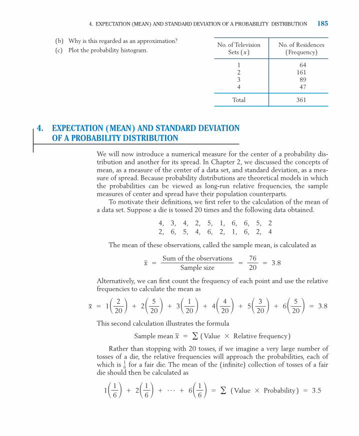
4. EXPECTATION (MEAN) AND STANDARD DEVIATION OF A PROBABILITY DISTRIBUTION
We will now introduce a numerical measure for the center of a probability dis-tribution and another for its spread. In Chapter 2, we discussed the concepts ofmean, as a measure of the center of a data set, and standard deviation, as a mea-sure of spread. Because probability distributions are theoretical models in whichthe probabilities can be viewed as long-run relative frequencies, the samplemeasures of center and spread have their population counterparts.
To motivate their definitions, we first refer to the calculation of the mean ofa data set. Suppose a die is tossed 20 times and the following data obtained.
4, 3, 4, 2, 5, 1, 6, 6, 5, 22, 6, 5, 4, 6, 2, 1, 6, 2, 4
The mean of these observations, called the sample mean, is calculated as
Alternatively, we can first count the frequency of each point and use the relativefrequencies to calculate the mean as
This second calculation illustrates the formula
Sample mean ( Value � Relative frequency)
Rather than stopping with 20 tosses, if we imagine a very large number oftosses of a die, the relative frequencies will approach the probabilities, each ofwhich is for a fair die. The mean of the (infinite) collection of tosses of a fairdie should then be calculated as
( Value � Probability ) � 3.51 � 16 � � 2 � 1
6 � � ��� � 6 � 16 � � �
16
x � �
x � 1 � 220 � � 2 � 5
20 � � 3 � 120 � � 4 � 4
20 � � 5 � 320 � � 6 � 5
20 � � 3.8
x �Sum of the observations
Sample size�
7620
� 3.8
4. EXPECTATION (MEAN) AND STANDARD DEVIATION OF A PROBABILITY DISTRIBUTION 185
(b) Why is this regarded as an approximation?
(c) Plot the probability histogram.No. of Television No. of Residences
Sets (x ) (Frequency)
1 642 1613 894 47
Total 361
c05.qxd 10/15/09 11:04 AM Page 185

Motivated by this example and the stability of long-run relative frequency, it isthen natural to define the mean of a random variable X or its probability distri-bution as
� ( Value � Probability ) or � f ( )
where ’s denote the distinct values of X. The mean of a probability distribu-tion is also called the population mean for the variable X and is denoted by theGreek letter m.
The mean of a random variable X is also called its expected value and, alter-natively, denoted by E (X ). That is, the mean m and expected value E (X ) arethe same quantity and will be used interchangeably.
Example 8 Calculating the Population Mean Number of HeadsWith X denoting the number of heads in three tosses of a fair coin, calculatethe mean of X.
SOLUTION The probability distribution of X was recorded in Table 1. From the calcula-tions exhibited in Table 6 we find that the mean is 1.5.
The mean of a probability distribution has a physical interpretation. If ametal sheet is cut in the shape of the probability histogram, then m representsthe point on the base at which the sheet will balance. For instance, the meanm � 1.5 calculated in Example 8 is exactly at the center of mass for thedistribution depicted in Figure 1. Because the amount of probability corre-sponds to the amount of mass in a bar, we interpret the balance point m asthe center of the probability distribution.
Like many concepts of probability, the idea of the mean or expectation orig-inated from studies of gambling. When X refers to the financial gain in a gameof chance, such as playing poker or participating in a state lottery, the name “ex-pected gain” is more appealing than “mean gain.” In the realm of statistics, boththe names “mean” and “expected value” are widely used.
xi
xixi
186 CHAPTER 5/PROBABILITY DISTRIBUTIONS
The mean of X or population mean
Here the sum extends over all the distinct values xi of X.
� � ( Value � Probability ) � � xi f ( xi )
E ( X ) �
c05.qxd 10/15/09 11:04 AM Page 186

Example 9 Expected Value—Setting a PremiumA trip insurance policy pays $2000 to the customer in case of a loss due totheft or damage on a five-day trip. If the risk of such a loss is assessed to be 1in 200, what is the expected cost, per customer, to cover?
SOLUTION The probability that the company will be liable to pay $2000 to a customeris Therefore, the probability distribution of X, the payment percustomer, is as follows.
We calculate
The company’s expected cost per customer is $10.00 and, therefore, a pre-mium equal to this amount is viewed as the fair premium. If this premium ischarged and no other costs are involved, then the company will neither make aprofit nor lose money in the long run. In practice, the premium is set at a higherprice because it must include administrative costs and intended profit.
� $10.00 E ( X ) � 0 � .995 � 2000 � .005
1200 � .005.
4. EXPECTATION (MEAN) AND STANDARD DEVIATION OF A PROBABILITY DISTRIBUTION 187
TABLE 6 Mean of theDistribution of Table 1
x f (x ) x f (x )
0 0
1
2
3
Total 1128
� 1.5 �
38
18
68
38
38
38
18
Payment x Probability f (x )
$0 .995$2000 .005
c05.qxd 10/15/09 11:04 AM Page 187

188 CHAPTER 5/PROBABILITY DISTRIBUTIONS
No Casino Game Has a Positive Expected Profit
Each year, thousands of visitors come to casinos to gamble. Although allcount on being lucky and a few indeed return with a smiling face, most leavethe casino with a light purse. But, what should a gambler’s expectation be?
Consider a simple bet on the red of a roulette wheel that has 18 red,18 black, and 2 green slots. This bet is at even money so a $10 wager onred has an expected profit of
The negative expected profit says we expect to lose an average of52.6¢ on every $10 bet. Over a long series of bets, the relative frequencyof winning will approach the probability and that of losing will ap-proach so a player will lose a substantial amount of money.
Other bets against the house have a similar negative expected profit.How else could a casino stay in business?
2038 ,
1838
E ( Profit ) � ( 10 )� 1838 � � ( �10 )� 20
38 � � �.526
© SuperStock, Inc.
c05.qxd 10/15/09 11:04 AM Page 188

The expected value of is obtained by multiplying each valueby the probability f ( ) and then summing these products. This
motivates the definition:
The variance of X is abbreviated as Var(X ) and is also denoted by . Thestandard deviation of X is the positive square root of the variance and is de-noted by sd(X ) or s (a Greek lower-case sigma. )
The variance of X is also called the population variance and s denotes thepopulation standard deviation.
s 2
� � ( xi � )2 f ( xi )
Variance of X � � ( Deviation )
2 � ( Probability )
xi( x i � )2( X � )
2
4. EXPECTATION (MEAN) AND STANDARD DEVIATION OF A PROBABILITY DISTRIBUTION 189
The concept of expected value also leads to a numerical measure for thespread of a probability distribution—namely, the standard deviation. When wedefine the standard deviation of a probability distribution, the reasoning paral-lels that for the standard deviation discussed in Chapter 2.
Because the mean m is the center of the distribution of X, we express varia-tion of X in terms of the deviation We define the variance of X as theexpected value of the squared deviation To calculate this expectedvalue, we note that
( X � )2 .X � .
WithTakes Value Probability
f ( )f ( )
� �� �� �
f ( )xk( xk � )
2
x2( x2 � ) 2
x1( x1 � ) 2
( X � ) 2
Variance and Standard Deviation of X
� sd (X ) � �√ Var (X )
2 � Var ( X ) � � ( xi � ) 2 f ( xi )
Example 10 Calculating a Population Variance and Standard DeviationCalculate the variance and the standard deviation of the distribution of Xthat appears in the left two columns of Table 7.
c05.qxd 10/15/09 11:04 AM Page 189

SOLUTION We calculate the mean m , the deviations and finallyThe details are shown in Table 7.
An alternative formula for often simplifies the numerical work (see Ap-pendix A2.2).
Example 11 Alternative Calculation of VarianceWe illustrate the alternative formula for using the probability distributionin Example 10. See Table 8.
2
2
sd ( X ) � � √1.2 � 1.095
Var ( X ) � 2 � 1.2
( x � )2 f ( x ) .( x � )
2,x � ,
190 CHAPTER 5/PROBABILITY DISTRIBUTIONS
TABLE 7 Calculation of Variance and Standard Deviation
x f (x ) x f (x)
0 .1 0 �2 4 .41 .2 .2 �1 1 .22 .4 .8 0 0 03 .2 .6 1 1 .24 .1 .4 2 4 .4
Total 1.0 2.0 � m 1.2 � s2
( x � ) 2 f ( x )( x � )
2( x � )
Alternative Formula for Hand Calculation
2 � � xi2 f ( xi
) � 2
TABLE 8 Calculation of Variance by the Alternative Formula
x f (x ) x f (x ) f (x)
0 .1 .0 .01 .2 .2 .22 .4 .8 1.63 .2 .6 1.84 .1 .4 1.6
Total 1.0 2.0 5.2� m � � f (x )x2
x2
c05.qxd 10/15/09 11:04 AM Page 190

The standard deviation s, rather than , is the appropriate measure ofspread. Its unit is the same as that of X. For instance, if X refers to income indollars, s will have the unit dollar, whereas has the rather artificial unit
.
Exercises
(dollar)22
2
� √1.2 � 1.095
� 1.2
2 � 5.2 � ( 2.0 )
2
4. EXPECTATION (MEAN) AND STANDARD DEVIATION OF A PROBABILITY DISTRIBUTION 191
5.32 A book club announces a sweepstakes in orderto attract new subscribers. The prizes and thecorresponding chances are listed here (typi-cally, the prizes are listed in bold print in anadvertisement flyer while the chances are en-tered in fine print or not mentioned at all).
Prize Chance
$50,000 1 in one million$ 5,000 1 in 250,000$ 100 1 in 5,000$ 20 1 in 500
Suppose you have just mailed in a sweepstakesticket and X stands for your winnings.
(a) List the probability distribution of X.(Caution: What is not listed is the chanceof winning nothing, but you can figurethat out from the given information.)
(b) Calculate your expected winnings.
5.33 Calculate the mean and standard deviation forthe probability distribution of Example 5.
5.34 Referring to Exercise 5.27, find the mean andstandard deviation of the number of customers.
5.35 A construction company submits bids fortwo projects. Listed here are the profit andthe probability of winning each project.
5.29 Given the following probability distributionconcerning Web sites visited almost every day:
(a) Construct the probability histogram.
(b) Find E(X ), , and s.
5.30 A wait person proposed a distribution for thenumber of meals served on a two-for-one deal.
Find the mean and standard deviation.
5.31 In bidding for a remodeling project, a carpen-ter determines that he will have a net profit of$5000 if he gets the contract and a net loss of$86 if his bid fails. If the probability of his get-ting the contract is .2, calculate his expectedreturn.
2
x f (x )
2 .34 .56 .18 .1
x f (x )
1 .12 .23 .34 .4
c05.qxd 10/15/09 11:04 AM Page 191

Assume that the outcomes of the two bids are independent.
Chance of Profit Winning Bid
Project A $ 75,000 .50Project B $120,000 .65
(a) List the possible outcomes (win/not win)for the two projects and find their proba-bilities.
(b) Let X denote the company’s total profitout of the two contracts. Determine theprobability distribution of X.
(c) If it costs the company $2000 forpreparatory surveys and paperwork forthe two bids, what is the expected netprofit?
5.36 Refer to Exercise 5.35, but suppose that theprojects are scheduled consecutively with A inthe first year and B in the second year. Thecompany’s chance of winning project A is still.50. Instead of the assumption of indepen-dence, now assume that if the company winsproject A, its chance of winning B becomes .80due to a boost of its image, whereas its chancedrops to .40 in case it fails to win A. Underthis premise, do parts (a–c).
5.37 Upon examination of the claims records of 280policy holders over a period of five years, an in-surance company makes an empirical determi-nation of the probability distribution of X �number of claims in five years.
(a) Calculate the expectedvalue of X.
(b) Calculate the standarddeviation of X.
192 CHAPTER 5/PROBABILITY DISTRIBUTIONS
x f (x )
0 .3151 .2892 .2013 .1144 .0635 .0126 .006
5.38 Suppose the probability distribution of a ran-dom variable X is given by the function
Calculate the mean and standard deviation ofthis distribution.
5.39 The probability distribution of a random vari-able X is given by the function
(a) Calculate the numerical probabilities andlist the distribution.
(b) Calculate the mean and standard devia-tion of X.
*5.40 Given here are the probability distributions oftwo random variables X and Y.
(a) From the X distribution, determine the distribution of the random variable 8 � 2X and verify that it coincides with the Y distribution. (Hence, identify
(b) Calculate the mean and standard deviationof X (call these and , respectively).
(c) From the Y distribution, calculate themean and standard deviation of Y (callthese and , respectively).
(d) If then according to the-ory, we must have the relations
and Verify these relations from your results inparts (b) and (c).
5.41 A salesman of small-business computer sys-tems will contact four customers during aweek. Each contact can result in either a sale,with probability .3, or no sale, with probability .7.
Y � � b � X .Y � a � b X
Y � a � b X,
s Ym Y
s Xm X
Y � 8 � 2 X. )
f ( x ) �1
84 �5x��
43 � x� for x � 0, 1, 2, 3
f ( x ) �1225
�1x for x � 1, 2, 3, 4
x f (x )
1 .12 .33 .44 .2
y f (y )
0 .22 .44 .36 .1
c05.qxd 10/15/09 11:04 AM Page 192

Assume that customer contacts are inde-pendent.
(a) List the elementary outcomes and assignprobabilities.
(b) If X denotes the number of computer sys-tems sold during the week, obtain theprobability distribution of X.
(c) Calculate the expected value of X.
5.42 Refer to Exercise 5.41. Suppose the computersystems are priced at $2000, and let Y denotethe salesman’s total sales (in dollars) during aweek.
(a) Give the probability distribution of Y.
(b) Calculate E (Y ) and see that it is thesame as 2000 � E(X ).
5.43 Definition: The median of a distribution is thevalue m0 of the random variable such that
and In other words, the probability at or below m0 is
P [ X � m0 ] � .5.P [ X � m0 ] � .5
5. SUCCESSES AND FAILURES—BERNOULLI TRIALS 193
5. SUCCESSES AND FAILURES—BERNOULLI TRIALS
Often, an experiment can have only two possible outcomes. Example 5 con-cerned individual students who either preferred Internet or television news. Theproportion of the population that preferred Internet news was .60. Also, onlytwo outcomes are possible for a single trial in the scenarios of Examples 1 and2. In all these circumstances, a simple probability model can be developed forthe chance variation in the outcomes. Moreover, the population proportion neednot be known as in the previous examples. Instead, the probability distributionwill involve this unknown population proportion as a parameter.
Sampling situations where the elements of a population have a dichotomyabound in virtually all walks of life. A few examples are:
Inspect a specified number of items coming off a production line and countthe number of defectives.Survey a sample of voters and observe how many favor an increase of publicspending on welfare.Analyze the blood specimens of a number of rodents and count how manycarry a particular viral infection.Examine the case histories of a number of births and count how many in-volved delivery by Cesarean section.
Selecting a single element of the population is envisioned as a trial of the (sam-pling) experiment, so that each trial can result in one of two possible outcomes.
at least .5, and the probability at or above m0 isat least .5. Find the median of the distributiongiven in Exercise 5.29.
5.44 Given the two probability distributions
(a) Construct probability histograms. Whichdistribution has a larger spread?
(b) Verify that both distributions have thesame mean.
(c) Compare the two standard deviations.
x f (x )
1 .22 .63 .2
y f ( y )
0 .11 .22 .43 .24 .1
c05.qxd 10/15/09 11:04 AM Page 193

Our ultimate goal is to develop a probability model for the number of outcomes inone category when repeated trials are performed.
An organization of the key terminologies, concerning the successive repeti-tions of an experiment, is now in order. We call each repetition by the simplername—a trial. Furthermore, the two possible outcomes of a trial are now as-signed the technical names success (S) and failure (F) just to emphasize thepoint that they are the only two possible results. These names bear no connota-tion of success or failure in real life. Customarily, the outcome of primary inter-est in a study is labeled success (even if it is a disastrous event). In a study of therate of unemployment, the status of being unemployed may be attributed thestatistical name success!
Further conditions on the repeated trials are necessary in order to arrive atour intended probability distribution. Repeated trials that obey these conditionsare called Bernoulli trials after the Swiss mathematician Jacob Bernoulli.
Perhaps the simplest example of Bernoulli trials is the prototype model oftossing a coin, where the occurrences head and tail can be labeled S and F, re-spectively. For a fair coin, we assign probability to success and to failure.
q � 12 p � 1
2
194 CHAPTER 5/PROBABILITY DISTRIBUTIONS
Boy or girl?
A model for the potential sex of a newborn is the assignment of probability toeach of the two outcomes. For most applications, .5 is assigned to “male” but exten-sive official statistics establish that the probability is actually about .52. BlaineHarrington/Photolibrary Group Limited.
c05.qxd 10/15/09 11:04 AM Page 194

Example 12 Sampling from a Population with Two Categories of ElementsConsider a lot (population) of items in which each item can be classified aseither defective or nondefective. Suppose that a lot consists of 15 items, ofwhich 5 are defective and 10 are nondefective.
Do the conditions for Bernoulli trials apply when sampling (1) with re-placement and (2) without replacement?
SOLUTION 1. Sampling with replacement. An item is drawn at random (i.e., ina manner that all items in the lot are equally likely to be selected).The quality of the item is recorded and it is returned to the lot be-fore the next drawing. The conditions for Bernoulli trials are satis-fied. If the occurrence of a defective is labeled S, we have
2. Sampling without replacement. In situation (2), suppose that 3items are drawn one at a time but without replacement. Then thecondition concerning the independence of trials is violated. Forthe first drawing, If the first draw produces S, the lotthen consists of 14 items, 4 of which are defective. Given this in-formation about the result of the first draw, the conditional proba-bility of obtaining an S on the second draw is then whichestablishes the lack of independence.
This violation of the condition of independence loses its thrust when thepopulation is vast and only a small fraction of it is sampled. Consider sam-pling 3 items without replacement from a lot of 1500 items, 500 of whichare defective. With S1 denoting the occurrence of an S in the first draw and S2that in the second, we have
and
P ( S2 � S1 ) �
4991499
P ( S1) �500
1500�
515
414 � 5
15 ,
P ( S ) � 515 .
P( S ) � 515 .
5. SUCCESSES AND FAILURES—BERNOULLI TRIALS 195
Bernoulli Trials
1. Each trial yields one of two outcomes, technically called success (S)and failure (F).
2. For each trial, the probability of success P(S) is the same and is de-noted by p � P(S). The probability of failure is then for each trial and is denoted by q, so that
3. Trials are independent. The probability of success in a trial remainsunchanged given the outcomes of all the other trials.
p � q � 1.P(F) � 1 � p
c05.qxd 10/15/09 11:04 AM Page 195

For most practical purposes, the latter fraction can be approximated by Strictly speaking, there has been a violation of the independence of trials, butit is to such a negligible extent that the model of Bernoulli trials can be as-sumed as a good approximation.
Example 12 illustrates the important points:
Example 13 further illustrates the kinds of approximations that are sometimesemployed when using the model of the Bernoulli trials.
Example 13 Testing a New Antibiotic—Bernoulli Trials?Suppose that a newly developed antibiotic is to be tried on 10 patients whohave a certain disease and the possible outcomes in each case are cure (S) orno cure (F).
Comment on the applicability of the Bernoulli trial model.
SOLUTION Each patient has a distinct physical condition and genetic constitution thatcannot be perfectly matched by any other patient. Therefore, strictly speak-ing, it may not be possible to regard the trials made on 10 different patientsas 10 repetitions of an experiment under identical conditions, as the defini-tion of Bernoulli trials demands. We must remember that the conditions of aprobability model are abstractions that help to realistically simplify the com-plex mechanism governing the outcomes of an experiment. Identificationwith Bernoulli trials in such situations is to be viewed as an approximation ofthe real world, and its merit rests on how successfully the model explainschance variations in the outcomes.
515 .
196 CHAPTER 5/PROBABILITY DISTRIBUTIONS
If elements are sampled from a dichotomous population at random andwith replacement, the conditions for Bernoulli trials are satisfied.
When the sampling is made without replacement, the condition ofthe independence of trials is violated. However, if the population is largeand only a small fraction of it (less than 10%, as a rule of thumb) is sam-pled, the effect of this violation is negligible and the model of theBernoulli trials can be taken as a good approximation.
c05.qxd 10/15/09 11:04 AM Page 196

Exercises
5. SUCCESSES AND FAILURES—BERNOULLI TRIALS 197
(b) After each draw, the selected candy is notreturned to the jar.
(c) After each draw, the selected candy is re-turned to the jar and one new candy ofthe same color is added in the jar.
5.48 Refer to Exercise 5.47 and suppose insteadthat the mix consists of 2500 candies, of which600 are brown, 1200 are yellow, and 700 areof other colors. Repeat parts (a–c) of Exercise5.47 in this setting.
5.49 From four agricultural plots, two will be se-lected at random for a pesticide treatment. Theother two plots will serve as controls. For eachplot, denote by S the event that it is treatedwith the pesticide. Consider the assignment oftreatment or control to a single plot as a trial.
(a) Is P(S) the same for all trials? If so, whatis the numerical value of P(S)?
(b) Are the trials independent? Why or whynot?
5.50 Refer to Exercise 5.49. Now suppose for eachplot a fair coin will be tossed. If a head showsup, the plot will be treated; otherwise, it willbe a control. With this manner of treatment al-location, answer parts (a) and (b).
5.51 A market researcher intends to study the con-sumer preference between regular and decaf-feinated coffee. Examine the plausibility of themodel of Bernoulli trials in the following situa-tions.
(a) One hundred consumers are randomly se-lected and each is asked to report thetypes of coffee (regular or decaffeinated)purchased in the five most recent occa-sions. If we consider each purchase as atrial, this inquiry deals with 500 trials.
(b) Five hundred consumers are randomly se-lected and each is asked about the mostrecent purchase of coffee. Here again theinquiry deals with 500 trials.
5.52 A backpacking party carries three emergencysignal flares, each of which will light with a
5.45 Is the model of Bernoulli trials plausible ineach of the following situations? Discuss inwhat manner (if any) a serious violation of theassumptions can occur.
(a) Seven friends go to a blockbuster movieand each is asked whether the movie wasexcellent.
(b) A musical aptitude test is given to 10 stu-dents and the times to complete the testare recorded.
(c) Items coming off an assembly line are in-spected and classified as defective or non-defective.
(d) Going house by house down the blockand recording if the newspaper was deliv-ered on time.
5.46 In each case, examine whether or not repeti-tions of the stated experiment conform to themodel of Bernoulli trials. Where the model isappropriate, determine the numerical value ofp or indicate how it can be determined.
(a) Roll a fair die and observe the numberthat shows up.
(b) Roll a fair die and observe whether or notthe number 6 shows up.
(c) Roll two fair dice and observe the total ofthe points that show up.
(d) Roll two fair dice and observe whether ornot both show the same number.
(e) Roll a loaded die and observe whether ornot the number 6 shows up.
5.47 A jar contains 25 candies of which 6 arebrown, 12 are yellow, and 7 are of other colors.Consider 4 successive draws of 1 candy at ran-dom from the jar and suppose the appearanceof a yellow candy is the event of interest. Foreach of the following situations, state whetheror not the model of Bernoulli trials is reason-able, and if so, determine the numerical valueof p.
(a) After each draw, the selected candy is re-turned to the jar.
c05.qxd 10/15/09 11:04 AM Page 197

6. THE BINOMIAL DISTRIBUTION
This section deals with a basic distribution that models chance variation in repe-titions of an experiment that has only two possible outcomes. The random vari-able X of interest is the frequency count of one of the categories. Previously, itsdistribution was calculated under the assumption that the population propor-tion is known. For instance, the probability distribution of Table 3, from Exam-ple 5, resulted from the specification that 60% of the population of students
probability of .98. Assuming that the flares op-erate independently, find:
(a) The probability that at least one flare lights.
(b) The probability that exactly two flares light.
5.53 Consider Bernoulli trials with success probabil-ity
(a) Find the probability that four trials resultin all failures.
(b) Given that the first four trials result in allfailures, what is the conditional probabilitythat the next four trials are all successes?
(c) Find the probability that the first successoccurs in the fourth trial.
5.54 If in three Bernoulli trials P [All three are suc-cesses] � .064, what is the probability that allthree are failures?
5.55 According to the U. S. Census Bureau, in 2007about 10% of persons between 25 and 30 yearsold live alone. Let S be the event a person livesalone. If five persons in that age group are ran-domly selected,
(a) Find the probability of the sequence SFFSF.
(b) Find the probability of exactly 2 S's.
5.56 A graphic designer makes a presentation toclients and this results in sales of her servicesin one-fourth of the cases. Assuming the re-sults for different clients are independent
(a) Find the probability that exactly 3 of thenext 4 presentations will result in sales.
(b) Find the probability that none of the pre-sentations result in a sale.
5.57 An animal either dies (D) or survives (S) in thecourse of a surgical experiment. The experimentis to be performed first with two animals. If both
p � .3.
198 CHAPTER 5/PROBABILITY DISTRIBUTIONS
survive, no further trials are to be made. If ex-actly one animal survives, one more animal is toundergo the experiment. Finally, if both animalsdie, two additional animals are to be tried.
(a) List the sample space.
(b) Assume that the trials are independentand the probability of survival in each trialis Assign probabilities to the elementaryoutcomes.
(c) Let X denote the number of survivors.Obtain the probability distribution of Xby referring to part (b).
5.58 The accompanying table shows the percent-ages of residents in a large community whenclassified according to gender and presence of aparticular allergy.
Suppose that the selection of a person is con-sidered a trial and the presence of the allergy isconsidered a success. For each case, identify thenumerical value of p and find the requiredprobability.
(a) Four persons are selected at random.What is the probability that none has theallergy?
(b) Four males are selected at random. What isthe probability that none has the allergy?
(c) Two males and two females are selectedat random. What is the probability thatnone has the allergy?
14 .
AllergyPresent Absent
Male 16 36Female 9 39
c05.qxd 10/15/09 11:04 AM Page 198

6. THE BINOMIAL DISTRIBUTION 199
prefer news from the Internet. In a practical situation, however, the popu-lation proportion is usually an unknown quantity. When this is so, the probabil-ity distribution of X cannot be numerically determined. However, we will seethat it is possible to construct a model for the probability distribution of X thatcontains the unknown population proportion as a parameter. The probabilitymodel serves as the major vehicle of drawing inferences about the populationfrom observations of the random variable X.
Consider a fixed number n of Bernoulli trials with the success probability pin each trial. The number of successes obtained in n trials is a random variablethat we denote by X. The probability distribution of this random variable X iscalled a binomial distribution.
The binomial distribution depends on the two quantities n and p. For in-stance, the distribution appearing in Table 1 is precisely the binomial distribu-tion with and whereas that in Table 3 is the binomial distribu-tion with and
A review of the developments in Example 5 will help motivate a formulafor the general binomial distribution.
Example 14 Example 5 Revisited—An Example of the Binomial DistributionThe random variable X represents the number of students who prefernews from the Internet among a random sample of students from an � 4
p � .6.n � 4p � .5,n � 3
A probability model is an assumed form of the probability distributionthat describes the chance behavior for a random variable X.
Probabilities are expressed in terms of relevant population quantities,called the parameters.
The Binomial Distribution
Denote
The random variable X is called a binomial random variable. Its distribu-tion is called a binomial distribution.
X � the (random) number of successes in n trials
p � the probability of success in each trial
n � a fixed number of Bernoulli trials
c05.qxd 10/15/09 11:04 AM Page 199

large university. Instead of the numerical value .6, we now denote the pop-ulation proportion of students who prefer Internet news by the symbol p.Furthermore, we relabel the outcome “Internet” as a success ( S ) and “notInternet” as a failure ( F ). The elementary outcomes of sampling 4 stu-dents, the associated probabilities, and the value of X are listed as follows.
FFFF SFFF SSFF SSSF SSSSFSFF SFSF SSFSFFSF SFFS SFSSFFFS FSSF FSSS
FSFSFFSS
Because the population of students at a large university is vast, the trials canbe treated as independent. Also, for an individual trial, and
The event has one outcome, FFFF, whoseprobability is
To arrive at an expression for we consider the outcomes listedin the second column. The probability of SFFF is
and the same result holds for every outcome in this column. There are 4 out-comes so we obtain The factor 4 is the number ofoutcomes with one S and three F’s. Even without making a complete list ofthe outcomes, we can obtain this count. Every outcome has 4 places and the 1place where S occurs can be selected from the total of 4 in ways,
while the remaining 3 places must be filled with an F. Continuing in the sameline of reasoning, we see that the value occurs with
outcomes, each of which has a probability of . Therefore
.After we work out the remaining terms, the binomial distribution with trials can be presented as in Table 9.n � 4
p2 q2�2
4�P [ X � 2 ] �p2
q2�2
4� � 6X � 2
�14� � 4
P [ X � 1 ] � 4 p q
3.
P ( SFFF ) � p � q � q � q � p q3
P [X � 1 ],
P[X � 0 ] � P ( FFFF ) � q � q � q � q � q4
[ X � 0 ]P ( F ) � q � 1 � p.P ( S ) � p
200 CHAPTER 5/PROBABILITY DISTRIBUTIONS
Value of X 0 1 2 3 4
Probability of each outcome
1 4 6 4 1Number of outcomes
� �44�� �4
3�� �42�� �4
1�� �40�
p 4p3
qp2 q2p q3q4
c05.qxd 10/15/09 11:04 AM Page 200

It would be instructive for the reader to verify that the numerical proba-bilities appearing in Table 3 are obtained by substituting p � .6 and q � .4in the entries of Table 9.
Extending the reasoning of Example 14 to the case of a general number n ofBernoulli trials, we observe that there are outcomes that have exactly xsuccesses and failures. The probability of every such outcome is .Therefore,
for 1, . . . , n
is the formula for the binomial probability distribution with n trials.
Example 15 The Binomial Distribution and GeneticsAccording to the Mendelian theory of inherited characteristics, a cross fertil-ization of related species of red- and white-flowered plants produces a gener-ation whose offspring contain 25% red-flowered plants. Suppose that a horti-culturist wishes to cross 5 pairs of the cross-fertilized species. Of the resulting5 offspring, what is the probability that:
(a) There will be no red-flowered plants?
(b) There will be 4 or more red-flowered plants?
SOLUTION Because the trials are conducted on different parent plants, it is natural to as-sume that they are independent. Let the random variable X denote the number
x � 0,f ( x ) � P [ X � x ] � �nx� px qn�x
px qn�xn � x�n
x�
6. THE BINOMIAL DISTRIBUTION 201
TABLE 9 Binomial Distribution with n � 4 Trials
Value x 0 1 2 3 4
Probability f (x) p4 q0�4
4�p3 q1�4
3�p2 q2�4
2�p1 q3�4
1�p0 q4�4
0�
The binomial distribution with n trials and success probability p is described by the function
for the possible values x � 0, 1,� � � , n.
f ( x ) � P [ X � x ] � �nx� px( 1 � p )n�x
c05.qxd 10/15/09 11:04 AM Page 201

of red-flowered plants among the 5 offspring. If we identify the occurrenceof a red as a success S, the Mendelian theory specifies that P (S) �p � and hence X has a binomial distribution with and The required probabilities are therefore
(a)
(b)
To illustrate the manner in which the values of p influence the shape of thebinomial distribution, the probability histograms for three binomial distribu-tions with and p values of .5, .3, and .7, respectively, are presented inFigure 3. When the binomial distribution is symmetric with the high-est probability occurring at the center (see Figure 3a).
For values of p smaller than .5, more probability is shifted toward thesmaller values of x and the distribution has a longer tail to the right. Figure 3b,where the binomial histogram for is plotted, illustrates this tendency.On the other hand, Figure 3c with illustrates the opposite tendency:The value of p is higher than .5, more probability mass is shifted toward highervalues of x, and the distribution has a longer tail to the left. Considering the his-tograms in Figures 3b and 3c, we note that the value of p in one histogram is thesame as the value of q in the other. The probabilities in one histogram are ex-actly the same as those in the other, but their order is reversed. This illustrates ageneral property of the binomial distribution: When p and q are interchanged,the distribution of probabilities is reversed.
p � .7p � .3
p � .5,n � 6
� .015 � .001 � .016
P [ X � 4 ] � f (4) � f (5) � �54� (.25)4 (.75)1 � �5
5� (.25)5 (.75)0
P [ X � 0 ] � f ( 0 ) � ( .75 )5 � .237
p � .25.n � 514 ,
202 CHAPTER 5/PROBABILITY DISTRIBUTIONS
.016
0 1 2 3 4 5 6 x 0 1 2 3 4 5 6 x 0 1 2 3 4 5 6 x
p = .5 p = .3 p = .7
.016
.093 .093
.235 .235
.312
.118 .118
.302 .302.324 .324
.186 .186
.059 .059
.010 .010.001 .001
(a) (b) (c)
Figure 3 Binomial distributions for n � 6.
c05.qxd 10/15/09 11:04 AM Page 202

How to Use the Binomial Table (Appendix B, Table 2)
Although the binomial distribution is easily evaluated on a computer and somehand calculators, we provide a short table in Appendix B, Table 2. It covers se-lected sample sizes n ranging from 1 to 25 and several values of p. For a givenpair (n, p), the table entry corresponding to each c represents the cumulative
probability as is explained in the following scheme.
The probability of an individual value x can be obtained from this table by asubtraction of two consecutive entries. For example,
Example 16 Binomial Distribution for the Number CuredSuppose it is known that a new treatment is successful in curing a muscularpain in 50% of the cases. If it is tried on 15 patients, find the probability that:
(a) At most 6 will be cured.
(b) The number cured will be no fewer than 6 and no more than 10.
(c) Twelve or more will be cured.
SOLUTION Designating the cure of a patient by S and assuming that the results for indi-vidual patients are independent, we note that the binomial distribution with
and is appropriate for number of patients who arecured. To compute the required probabilities, we consult the binomial tablefor and p � .5.n � 15
X �p � .5n � 15
P [ X � 2 ] � f ( 2 ) � �table entry atc � 2 � � �table entry at
c � 1 �
P[ X � c ] � �c
x � 0 f ( x ),
6. THE BINOMIAL DISTRIBUTION 203
The Binomial Distribution
Value x Probability f (x )
0 f (0)1 f (1)2 f (2)� �� �� �n f (n )
Total 1
Appendix B, Table 2 provides
c Table Entry
0 f (0)1 f (0) + f (1)2 f (0) + f (1) + f (2)� �� �� �n 1.000
�c
x � 0 f ( x ) � P [ X � c ]
c05.qxd 10/15/09 11:04 AM Page 203

(a) which is directly obtained by reading fromthe row
(b) We are to calculate
The table entry corresponding to gives
and the entry corresponding to yields
Because their difference represents the sum we obtain
(c) To find , we use the law of complement:
Note that is the same event as
(An Aside: Refer to our “muscular pain” example in Section 1 of Chapter4. The mystery surrounding the numerical probability .018 is now re-solved.)
The Mean and Standard Deviation of the Binomial Distribution
Although we already have a general formula that gives the binomial probabili-ties for any n and p, in later chapters we will need to know the mean and thestandard deviation of the binomial distribution. The expression np for the meanis apparent from the following intuitive reasoning: If a fair coin is tossed 100times, the expected number of heads is Likewise, if the proba-bility of an event is p, then in n trials the event is expected to happen np times.The formula for the standard deviation requires some mathematical derivation,which we omit.
100 � 12 � 50.
[ X � 11].[ X � 12 ]
� .018 � 1 � .982
P [ X � 12 ] � 1 � P [ X � 11 ]
P [ X � 12 ]
� .790 � .941 � .151
P [ 6 � X � 10 ] � P [ X � 10 ] � P [ X � 5 ]
�10
x � 6 f ( x ),
P [ X � 5 ] � �5
x � 0 f ( x ) � .151
c � 5
f ( x ) � .941P [ X � 10 ] � �10
x � 0
c � 10
� �10
x � 6 f ( x )
P [ 6 � X � 10 ] � f ( 6 ) � f ( 7 ) � f ( 8 ) � f ( 9 ) � f ( 10 )
c � 6.P [ X � 6 ] � .304,
204 CHAPTER 5/PROBABILITY DISTRIBUTIONS
c05.qxd 10/15/09 11:04 AM Page 204

Example 17 Calculating the Population Mean and Standard Deviation of a Binomial DistributionFor the binomial distribution with and calculate the meanand the standard deviation.
SOLUTION Employing the formulas, we obtain
The mean agrees with the results of Example 8. The reader may wish to checkthe standard deviation by numerical calculations using the definition of s.
Exercises
sd � √ n p q � √ 3 � .5 � .5 � √ .75 � .866
Mean � n p � 3 � .5 � 1.5
p � .5,n � 3
6. THE BINOMIAL DISTRIBUTION 205
The binomial distribution with n trials and success probability p has
sd � √ n p q
Variance � n p q (Recall: q � 1 � p)
Mean � n p
5.59 For each situation, state whether or not a bino-mial distribution holds for the random variableX. Also, identify the numerical values of n andp when a binomial distribution holds.
(a) A fair die is rolled 10 times, and X de-notes the number of times 6 shows up.
(b) A fair die is rolled until 6 appears, and Xdenotes the number of rolls.
(c) In a jar, there are ten marbles, of which fourare numbered 1, three are numbered 2,two are numbered 3, and one is numbered4. Three marbles are drawn at random, oneafter another and with replacement, and Xdenotes the count of the selected marblesthat are numbered either 1 or 2.
(d) The same experiment as described in part(c), but now X denotes the sum of thenumbers on the selected marbles.
5.60 Construct a tree diagram for three Bernoullitrials. Attach probabilities in terms of p and q
to each outcome and then table the binomialdistribution for
5.61 In each case, find the probability of x successesin n Bernoulli trials with success probability pfor each trial.
(a)
(b)
(c)
5.62 (a) Plot the probability histograms for the bi-nomial distributions for and pequal to .2, .5, and .8.
(b) Locate the means.
(c) Find for each of the threecases.
5.63 An interior designer makes a presentation topotential clients and this results in sales of herservices in 35% of the cases. Let X denote the
P [ X � 4 ]
n � 5
x � 2 n � 6 p � .75
x � 3 n � 6 p � .25
x � 2 n � 3 p � .35
n � 3.
c05.qxd 10/15/09 11:04 AM Page 205
number of sales in the next four presentations.Assuming the results for different clients areindependent, calculate the probabilities
for 1, . . . , 5and find
(a)
(b)
(c)
5.64 Refer to Exercise 5.63. What is the mostprobable value of X (called the mode of adistribution)?
5.65 About 75% of dog owners buy holiday pre-sents for their dogs. Suppose n = 4 dog own-ers are randomly selected. Find the probabilitythat
(a) three or more buy their dog holiday pre-sents.
(b) at most three buy their dog holiday pre-sents
(c) Find the expected number of persons, inthe sample, who buy their dog holidaypresents.
5.66 According to a recent survey, outside of theirown family members, 26% of adult Americanshave no close friend to confide in. If this is theprevailing probability today, find the probabil-ity that in a random sample of n = 5 adults
(a) two or more have no close friend.
(b) at most two have no close friend.
(c) Find the expected number of personswho have no close friend.
5.67 Suppose 15% of the trees in a forest have se-vere leaf damage from air pollution. If 5 treesare selected at random, find the probabilitythat:
(a) Three of the selected trees have severeleaf damage.
(b) No more than two have severe leaf dam-age.
5.68 Rh-positive blood appears in 85% of the whitepopulation in the United States. If 8 people are
1
P [ X � 2 or 4 ]
P [ X � 3 ]
P [ X � 3 ]
x � 0,f ( x ) � P [ X � x ]
206 CHAPTER 5/PROBABILITY DISTRIBUTIONS
sampled at random from that population, findthe probability that:
(a) At least 6 of them have Rh-positiveblood.
(b) At most 3 of them have Rh-negativeblood, that is, an absence of Rh positive.
5.69 Using the binomial table, find the probabilityof:
(a) Four successes in 13 trials when
(b) Eight failures in 13 trials when
(c) Eight successes in 13 trials when
Explain why you get identical answers in parts(b) and (c).
5.70 According to the U.S. Census Bureau, in 2007about 10% of persons between 25 and 30 yearsold live alone. For a random sample of size n,use the binomial table to find the probability of
(a) 1 or fewer persons living alone when n =12.
(b) 2 or more persons living alone when n =12.
(c) Find the expected number when n = 12.
(d) 1 or fewer persons living alone when n =20.
5.71 About 30% of adults say that reading is a fa-vorite leisure activity. Let success be the out-come that reading is a favorite leisure activity.Find the probability that
(a) More than 5 trials are needed in orderto obtain 3 successes. (Hint: In otherwords, the event is: at most 2 successesin 5 trials.)
(b) More than 9 trials are needed in order toobtain 5 successes.
5.72 A survey report states that 70% of adultwomen visit their doctors for a physical exami-nation at least once in two years. If 20 adultwomen are randomly selected, find the proba-bility that
(a) Fewer than 14 of them have had a physi-cal examination in the past two years.
(b) At least 17 of them have had a physicalexamination in the past two years.
p � .3.
p � .7.
p � .3.
75% is between the two 2008 survey results obtained by theAmerican Kennel Club and Harris Interactive Poll.
1
c05.qxd 10/15/09 11:04 AM Page 206

5.73 Calculate the mean and standard deviation ofthe binomial distribution using the formulas in mean = np
(a) Exercise 5.65 if n is changed to 20.
(b) Exercise 5.70 when n = 20.
(c) Exercise 5.71 when n = 40.
5.74 (a) For the binomial distribution withand list the probability
distribution (x, f (x )) in a table.
(b) From this table, calculate the mean andstandard deviation by using the methodsof Section 4.
(c) Check your results with the formulasmean � np, sd �
5.75 Suppose that 20% of the college seniors sup-port an increase in federal funding for care ofthe elderly. If 20 college seniors are randomlyselected, what is the probability that at most 3of them support the increased funding?
5.76 Referring to Exercise 5.75, find:
(a) The expected number of college seniors,in a random sample of 20, supporting theincreased funding.
(b) The probability that the number of sam-pled college seniors supporting the in-creased funding equals the expectednumber.
5.77 According to a recent report of the AmericanMedical Association, 9.0% of practicing physi-cians are in the specialty area of family prac-tice. Assuming that the same rate prevails, findthe mean and standard deviation of the num-ber of physicians specializing in family practiceout of a current random selection of 545 med-ical graduates.
5.78 According to the Mendelian theory of inheri-tance of genes, offspring of a dihybrid cross ofpeas could be any of the four types: round-yellow (RY ), wrinkled-yellow (WY ), round-green (RG ) and wrinkled-green (WG ), andtheir probabilities are in the ratio 9 :3 :3 :1.
(a) If X denotes the number of RY offspringfrom 130 such crosses, find the mean andstandard deviation of X.
√ n p q.
p � .6,n � 3
s d � √ n p (1�p)
6. THE BINOMIAL DISTRIBUTION 207
(b) If Y denotes the number of WG offspringfrom 85 such crosses, find the mean andstandard deviation of Y.
5.79 The following table (see Exercise 5.58) showsthe percentages of residents in a large commu-nity when classified according to gender andpresence of a particular allergy. For each partbelow, find the mean and standard deviation ofthe specified random variable.
(a) X stands for the number of persons hav-ing the allergy in a random sample of 40persons.
(b) Y stands for the number of males havingthe allergy in a random sample of 40males.
(c) Z stands for the number of females nothaving the allergy in a random sample of40 females.
The Following Exercise Requires a Computer
5.80 Many computer packages produce binomialprobabilities. We illustrate the MINITAB com-mands for obtaining the binomial probabilitieswith n � 5 and p � .33. The probabilities P [X � x ] are obtained by first setting 0, 1, 2,3, 4, 5 in C1 and then selecting:
Allergy
Present Absent
Male 16 36Female 9 39
Calc Probability distributions.
Type 5 in Number of trials
and .33 in Probability.
Enter C1 in Input constant. Click OK.
c05.qxd 10/15/09 11:04 AM Page 207

7. THE BINOMIAL DISTRIBUTION IN CONTEXT
Requests for credit cards must be processed to determine if the applicantmeets certain financial standards. In many instances, such as when the applicantalready has a long-term good credit record, only a short review is required.
which produces the output
Probability Density Function
Binomial with n � 5 and p � 0.33
x P(X=x)
0 0.135013
1 0.332493
2 0.327531
3 0.161321
4 0.039728
5 0.003914
To obtain the cumulative probabilities P (X � x ), click Cumulative probability in-stead of Probability. The resulting output is
208 CHAPTER 5/PROBABILITY DISTRIBUTIONS
Cumulative Distribution Function
Binomial with n � 5 and p � 0.33
x P(X<=x)
0 0.13501
1 0.46751
2 0.79504
3 0.95636
4 0.99609
5 1.00000
Using the computer, calculate
(a) and whenand
(b) when andn � 35
p � .43P [ 10 � X � 15 ]
n � 12p � .67P [ X � 8 ]P [ X � 8 ]
Poor Linus. Chance did not even favor him with half correct. Reprinted by permission of United Features Syndicate, Inc.© 1968.
c05.qxd 10/15/09 11:04 AM Page 208

7. THE BINOMIAL DISTRIBUTION IN CONTEXT 209
Usually this consists of a credit score assigned on the basis of the answers toquestions on the application and then a computerized check of credit records.Many other cases require a full review with manual checks of information to de-termine the credit worthiness of the applicant.
Each week, a large financial institution selects a sample of 20 incomingapplications and counts the number requiring full review. From data collectedover several weeks, it is observed that about 40% of the applications requirefull review. If we take this long-run relative frequency as the probability, whatis an unusually large number of full reviews and what is an unusually smallnumber?
Let X be the number in the sample that require a full review. From the bi-nomial table, with and we get
Taken together, the probability of X being 3 or less or 13 or more is .037, sothose values should occur less than four times in 100 samples. That is, theycould be considered unusual. In Exercise 5.81, you will be asked to show thateither including 4 or including 12 will lead to a combined probability greaterthan .05. That is, the large and small values should then occur more than 1 in 20times. For many people, this would be too frequent to be considered rare or un-usual.
For the count X, we expect applications in the sam-ple to require a full review. The standard deviation of this count is
Alternatively, when n is moderate or large, wecould describe as unusual two or more standard deviations from the mean. Avalue at least two standard deviations, or 2(2.191) � 4.382, above the meanof 8 must be 13 or more. A value 2 or more standard deviations below the meanmust be 3 or less. These values correspond exactly to the values above thatwhich we called unusual. In other cases, the two standard deviations approachprovides a reasonable and widely used approximation.
p Charts for Trend
A series of sample proportions should be visually inspected for trend. A graphcalled a p chart helps identify times when the population proportion has changedfrom its long-time stable value. Because many sample proportions will be graphed,it is customary to set control limits at 3 rather than 2 standard deviations.
When p0 is the expected or long-run proportion, we obtain a lower controllimit by dividing the lower limit for X, by the samplesize. Doing the same with the upper bound, we obtain an upper control limit.
Lower control limit Upper control limit
p0 � 3� p0 ( 1 � p0
)
np0 � 3� p0
( 1 � p0 )
n
n p0 � 3√n p0 ( 1 � p0
),
√ 20 ( .4 )( 1 � .4 ) � 2.191.
n p � 20 � .4 � 8
P [ X � 13 ] � 1 � P [ X � 12 ] � 1 � .979 � .021
P [ X � 3 ] � .016
p � .4,n � 20
c05.qxd 10/15/09 11:04 AM Page 209

In the context of credit applications that require a full review, .4 � p0 , so thecontrol limits are
The centerline is drawn as a solid line at the expected or long-run proportionand the two control limits each at a distance of three standard devia-
tions of the sample proportion from the centerline are also drawn as horizontallines as in Figure 4. Sample proportions that fall outside of the control limits areconsidered unusual and should result in a search for a cause that may include achange in the mix of type of persons requesting credit cards.
The number of applications requiring full review out of the 20 in the sam-ple were recorded for 19 weeks:
11 7 8 4 9 10 4 8 8 7 10 6 9 10 7 7 6 9 10
After converting to sample proportions by dividing by 20, we can graph thepoints in a p chart as in Figure 4. All the points are in control, and the financialinstitution does not appear to have reached the point where the mix of appli-cants includes more marginal cases.
p0 � .4,
p0 � 3� p0 (1 � p0
)
n� .4 � 3� .4 ( 1 � .4 )
20� .4 � 3 ( .110 ) � .73
p0 � 3� p0 (1 � p0
)
n� .4 � 3� .4 (1 � .4 )
20� .4 � 3 (.110 ) � .07
210 CHAPTER 5/PROBABILITY DISTRIBUTIONS
0.000
0.750
0.500
0.250
Pro
port
ion
0 5 10 15 20
Sample number
UCL = 0.73
= 0.40
LCL = 0.07
Figure 4 A p chart for the proportion of applications requiring afull review.
c05.qxd 10/15/09 11:04 AM Page 210

Exercises
USING STATISTICS WISELY 211
5.81 Refer to the credit card application approvalprocess on page 209 where unusual values aredefined.
(a) Show that if 4 is included as an unusualvalue, then the probability or
is greater than .05.
(b) Show that if 12 is included as an unusualvalue, then the probability or
is greater than .05.
5.82 Refer to the credit card application approvalprocess on page 209.
(a) Make a p chart using the centerline andcontrol limits calculated for
(b) Suppose the next five weeks bring 12, 10,15, 11, and 16 applications requiring fullreview. Graph the corresponding propor-tions on your p chart.
(c) Identify any weeks where the chart sig-nals “out of control.”
5.83 Several fast food restaurants advertise quarter-pound hamburgers. This could be interpretedas meaning half the hamburgers made have anuncooked weight of at least a quarter-poundand half have a weight that is less. An inspectorchecks 20 uncooked hamburgers at eachrestaurant.
p0 � .4.
X � 12 ]P [ X � 3
X � 13 ]P [ X � 4
USING STATISTICS WISELY
1. The assignment of a value to each possible outcome, which creates a ran-dom variable, should quantify an important feature of the outcomes.
2. Describe the chance behavior of a discrete random variable X by its proba-bility distribution
for each possible value x
3. Summarize a probability distribution, or the random variable, by its
Mean:
Variance: 2 � �all x
( x � )2 � f ( x )
� �all x
x � f ( x )
f ( x ) � P [X � x ]
(a) Make a p chart using the centerline andcontrol limits calculated for
(b) Suppose that five restaurants have 8, 11,7, 15, and 10 underweight hamburgers insamples of size 20. Graph the corre-sponding proportions on your p chart.
(c) Identify any restaurants where the chartsignals “out of control.”
5.84 Refer to Exercise 5.83.
(a) What are the unusual values for the num-ber of underweight hamburgers in thesample if they correspond to proportionsoutside of the control limits of the pchart?
(b) Use the binomial table to find the proba-bility of observing one of these unusualvalues.
5.85 Refer to Exercise 5.83. A syndicated newspa-per story reported that inspectors found 22 of24 hamburgers underweight at restaurant Wand fined that restaurant. Draw new controllimits on your chart, from Exercise 5.83, forone new sample of size 24. Plot the new pro-portion and determine if this point is “out ofcontrol.”
p0 � .5.
c05.qxd 10/15/09 11:04 AM Page 211

4. If the use of Bernoullie trials is reasonable, probabilities concerning thenumber of successes in n Bernoulli trials can be calculated using the for-mula for the binomial distribution
having mean np and variance np .
5. Never use the formula np(1 � p ) for the variance of a count of successesin n trials without first checking that the conditions for Bernoulli trials,independent trials with the same probability of success for each trial, hold.If the conditions are satisfied, then the binomial distribution is appropriate.
KEY IDEAS AND FORMULAS
The outcomes of an experiment are quantified by assigning each of them a nu-merical value related to a characteristic of interest. The rule for assigning thenumerical value is called a random variable X.
A random variable having a finite number of values, or a sequence of valueslike a count, is called discrete. If a random variable can take any value in aninterval, it is called a continuous random variable.
The probability distribution of X, or simply distribution, describes themanner in which probability is distributed over the possible values of X. Specifi-cally, it is a list or formula giving the pairs x and f (x ) � P [ X � x ].
A probability distribution serves as a model for explaining variation in apopulation.
A probability histogram graphically displays a discrete distribution usingbars whose area equals the probability.
A probability distribution has a
Mean
which is interpreted as the population mean. This quantity is also called the expected value E(X ). Although X is a variable, E ( X ) is a constant.
The population variance is
The standard deviation s is the positive square root of variance. The stan-dard deviation is a measure of the spread or variation of the population.
Bernoulli trials are defined by the characteristics: (1) two possible out-comes, success (S) or failure (F) for each trial; (2) a constant probability ofsuccess; and (3) independence of trials.
Sampling from a finite population without replacement violates the re-quirement of independence. If the population is large and the sample size small,the trials can be treated as independent for all practical purposes.
2 � E ( X � )2 � � ( x � )2 f ( x )
� � ( Value � Probability ) � � x f ( x )
( 1 � p )
f ( x ) � �
nx � p
x( 1 � p )n�x for x � 0,1, . . ., n
212 CHAPTER 5/PROBABILITY DISTRIBUTIONS
c05.qxd 10/15/09 11:04 AM Page 212

The number of successes X in a fixed number of Bernoulli trials is called abinomial random variable. Its probability distribution, called the binomial dis-tribution, is given by
for . . . , n
where number of trials, probability of success in each trial, and
The binomial distribution has
Mean � npStandard deviation �
A probability model is an assumed model for the probability distribution ofa random variable. Probabilities are expressed in terms of parameters which arefeatures of the population. For example, the binomial distribution is a probabil-ity model and the proportion p is a parameter.
A p chart displays sample proportions to reveal trends or changes in thepopulation proportion over time.
TECHNOLOGY
Calculating the binomial probabilities
MINITAB
Calculating the binomial probability
The following commands illustrate the calculation of underthe binomial distribution having
Dialog box:
Calc � Probability distributions � Binomial.Select Probability.Type 21 in Number of Trials and .57 in Probability of success.Select Input constant, and enter 14. Click OK.
Alternatively to get all of the binomial probabilities for you can first
Enter 0, 1, 2, . . ., 21 in C1.
Calc � Probability distributions � Binomial.Select Probability.Type 21 in Number of Trials and .57 in Probability of success.Then, instead of clicking Input constant,Enter C1 in Input column and C2 in Optional storage. Click OK.
n � 21,
n � 21 and p � .57:P [ X � 14 ]
P [ X � x ] � �
n
x� px( 1 � p ) n
�
x
P [ X � x ] and P [ X f x ]
√ n p q
q � 1 � p.p �n �
x � 0,f ( x ) � �nx� px qn�x
TECHNOLOGY 213
c05.qxd 10/15/09 11:04 AM Page 213

Calculating the cumulative binomial probability
Follow the same steps as in the calculation of the probability of single termsexcept:
Select Cumulative probability instead of Probability.Calc � Probability distributions � Binomial.Select Cumulative Probability.Type 21 in Number of trials and .57 in Probability of success.Select Input constant and enter 14. Click OK.
EXCEL
Calculating the binomial probability
We illustrate the calculation of under the binomial distribu-tion having .
With the cursor in a blank cell, select the fx icon, or select Insert and thenFunction. Choose Statistical and then BINOMDIST. Click OK.
Type 14 in Number_s, 21 in Trials, .57 in Probability_s, and False in Cumu-lative. Click OK.
Calculating the cumulative binomial probability
Follow the same steps as in the calculation of except:
Type True in Cumulative.
TI-84/-83 PLUS
Calculating the binomial probability
The following commands illustrate the calculation of underthe binomial distribution having :
Press 2ndVARS to read the probability distribution menu.Select 0:binompdf( and press ENTER.With binompdf( on the home screen, type 21, .57, 14) to give:
binompdf( 21, .57, 14)
Press ENTER.
2
n � 21 and p � .57P [ X � 14 ]
P [ X � x ] � �n x � px ( 1 � p )
n
�
x
P [X � x ]
P [ X f c ] � �c
x�0 �n
x � px ( 1 � p )
n
�
x
n � 21 and p � .57P [ X � 14 ]
P [ X � x ] � �
n
x� px ( 1 � p )n
�
x
P [ X f c ] � �c
x�0 �n
x � px ( 1 � p )n
�
x
214 CHAPTER 5/PROBABILITY DISTRIBUTIONS
The options O and A are different for some TI-84 calculators.2
c05.qxd 10/15/09 11:04 AM Page 214

Calculating the cumulative binomial probability
Follow the same steps as in the calculation of except replacethe second step by
Select A:binompdf( and press ENTER.
8. REVIEW EXERCISES
P [X � x ]
P [ X f c ] � �c
x�0 �n
x � px ( 1 � p )
n
�
x
8. REVIEW EXERCISES 215
5.86 Let X denote the difference (no. of heads �no. of tails) in three tosses of a coin.
(a) List the possible values of X.
(b) List the elementary outcomes associatedwith each value of X.
5.87 A large science department at the universitymade a list of its top 20 juniors and top 30 se-niors. The first list contains 8 females and thesecond 10 females. One person is randomly se-lected from each list and the two selections areindependent. Let X denote the number of fe-males selected.
(a) For each possible value of X, identify theelementary outcomes associated with thatvalue.
(b) Determine the probability distribution of X.
*5.88 Refer to Exercise 8.87 but now suppose thesampling is done in two stages: First a list is se-lected at random and then, from that list, twopersons are selected at random without re-placement. Let Y denote the number of fe-males in the sample.
(a) List the elementary outcomes concerningthe possible selections of this and the pos-sible compositions of the sample (use atree diagram). Find their probabilities.(Hint: Use conditional probability and themultiplication rule.)
(b) Determine the probability distribution of Y.
5.89 Refer to Exercise 5.87, but now suppose thatthe contents of the two lists are pooled to-
gether into a single larger list. Then two per-sons are drawn at random and without re-placement. Let W denote the number of fe-males in the sample. Obtain the probabilitydistribution of W.
*5.90 In a tennis championship, player A competesagainst player B in consecutive sets, and thegame continues until one player wins three sets.Assume that, for each set, P(A wins) � .4,P (B wins ) � .6, and the outcomes of differ-ent sets are independent. Let X stand for thenumber of sets played.
(a) List the possible values of X and identifythe elementary outcomes associated witheach value.
(b) Obtain the probability distribution ofX.
5.91 A list of the world's 10 largest companies, interms of value, contains 5 from the UnitedStates, 3 from China, and 1 each from Ger-many and The Netherlands. A potential in-vestor randomly selects 3 of the companies toresearch further.
(a) Find the probability distribution of X, thenumber of United States companies se-lected.
(b) Determine the mean and variance of X.
5.92 Refer to the monthly intersection accidentdata in Exercise 2.4. Considering an evenlonger record leads to a distribution for X =number of accidents in a month.
c05.qxd 10/15/09 11:04 AM Page 215

5.96 In the finals of a tennis match, the winner willget $60,000 and the loser $15,000. Find theexpected winnings of player B if (a) the twofinalists are evenly matched and (b) player Bhas probability .8 of winning.
5.97 The number of overnight emergency calls X tothe answering service of a heating and air con-ditioning firm have the probabilities .05, .1,.15, .35, .20, and .15 for 0, 1, 2, 3, 4, and 5calls, respectively.
(a) Find the probability of fewer than 3 calls.
(b) Determine E (X ) and sd(X ).
5.98 Suppose the number of parking tickets X is-sued during a police officer’s shift has theprobability distribution
x 0 1 2 3 4
f (x ) 0.13 0.14 0.43 0.20 0.10
(a) Find the mean and standard deviation ofthe number of parking tickets issued.
(b) Let andFind
(c) Suppose the numbers of tickets issued ondifferent days are independent. What isthe probability that, over the next fivedays, no parking tickets will be issued onexactly one of the days?
5.99 A botany student is asked to match the popu-lar names of three house plants with their ob-scure botanical names. Suppose the studentnever heard of these names and is trying tomatch by sheer guess. Let X denote the num-ber of correct matches.
(a) Obtain the probability distribution of X.
(b) What is the expected number of matches?
5.100 The number of days, X, that it takes the postoffice to deliver a letter between City A andCity B has the probability distribution
x f (x )
3 .54 .35 .2
2 � X � 1 ).P ( X �P (A �B ) �B � [ X � 1 ].A � [ X � 2 ]
(a) Calculate E (X ).
(b) Calculate sd(X ).
(c) Draw the probability histogram and lo-cate the mean.
5.93 The following distribution has been proposedfor the number of times a student will eat agourmet restaurant dinner next week.
(a) Calculate the mean and variance.
(b) Plot the probability histogram and locate m.
5.94 Refer to Exercise 5.92.
(a) List the x values that lie in the interval m � s to m � s and calculate
(b) List the x values that lie in the interval m � 2s to m � 2s and calculate
5.95 A student buys a lottery ticket for $1. Forevery 1000 tickets sold, two bicycles are to begiven away in a drawing.
(a) What is the probability that the studentwill win a bicycle?
(b) If each bicycle is worth $200, determinethe student’s expected gain.
P [ � 2 � X � � 2 ].
P [ � � X � � ].
216 CHAPTER 5/PROBABILITY DISTRIBUTIONS
x f (x )
0 .31 .42 .3
Value Probabilityx f (x )
0 .081 .202 .193 .244 .145 .136 .02
c05.qxd 10/15/09 11:04 AM Page 216

8. REVIEW EXERCISES 217
Find:
(a) The expected number of days.
(b) The standard deviation of the number ofdays.
5.101 A roulette wheel has 38 slots, of which 18 arered, 18 black, and 2 green. A gambler will playthree times, each time betting $5 on red. Thegambler gets $10 if red occurs and loses thebet otherwise. Let X denote the net gain of thegambler in 3 plays ( for instance, if he loses allthree times, then
(a) Obtain the probability distribution of X.
(b) Calculate the expected value of X.
(c) Will the expected net gain be different ifthe gambler alternates his bets betweenred and black? Why or why not?
5.102 Suppose that X can take the values 0, 1, 2, 3,and 4, and the probability distribution of X isincompletely specified by the function
for x � 0, 1, 2, 3
Find (a) f (4) (b) (c) E (X ) and(d) sd(X ).
5.103 The cumulative probabilities for a distribu-tion. A probability distribution can also bedescribed by a function that gives the accumu-lated probability at or below each value of X.Specifically,
Cumulative distribu-tion function at c �Sum of probabilitiesof all values
For the probabilitydistribution givenhere, we calculate
F ( 2 ) � P [ X � 2 ] � f ( 1 ) � f ( 2 ) � .19F ( 1 ) � P [ X � 1 ] � f ( 1 ) � .07
x � c
F ( c ) � P [X � c ] � �x � c
f ( x )
P [ X � 2 ]
f ( x ) �14
� 34 �
x
X � �15 ).
(a) Complete the F (x ) column in this table.
(b) Now cover the f (x ) column with a stripof paper. From the F (x ) values, recon-struct the probability function f (x ).
[Hint: f (x ) � F (x ) � F (x � 1).]
*5.104 Runs. In a row of six plants two are infectedwith a leaf disease and four are healthy. If werestrict attention to the portion of the samplespace for exactly two infected plants, themodel of randomness (or lack of contagion) as-sumes that any two positions, for the infectedplants in the row are as likely as any other.
(a) Using the symbols I for infected and Hfor healthy, list all possible occurrences oftwo I’s and four H’s in a row of 6.
(b) A random variable of interest is thenumber of runs X that is defined as thenumber of unbroken sequences of lettersof the same kind. For example, thearrangement IHHHIH has four runs,IIHHHH has two. Find the value of Xassociated with each outcome you listedin part (a).
(c) Obtain the probability distribution of Xunder the model of randomness.
*5.105 Refer to part (c) of Exercise 5.104. Calculatethe mean and standard deviation of X.
5.106 Let the random variable Y denote the propor-tion of times a head occurs in three tosses of acoin, that is, (No. of heads in 3 tosses) / 3.
(a) Obtain the probability distribution Y.
(b) Draw the probability histogram.
(c) Calculate the E (Y ) and sd(Y ).
5.107 Is the model of Bernoulli trials plausible ineach of the following situations? Identify anyserious violations of the conditions.
(a) A dentist records if each tooth in thelower jaw has a cavity or has none.
(b) Persons applying for a driver’s license willbe recorded as writing left- or right-handed.
Y �
(Note: There are �62� � 15 elementary outcomes.)
x f (x ) F (x )
1 .07 .072 .12 .193 .254 .285 .186 .10
c05.qxd 10/15/09 11:04 AM Page 217

(b) Find and E (X).
5.114 The probability that a voter will believe a ru-mor about a politician is .3. If 20 voters aretold individually:
(a) Find the probability that none of the 20believes the rumor.
(b) Find the probability that seven or morebelieve the rumor.
(c) Determine the mean and standard devia-tion of the number who believe the rumor.
5.115 National safety statistics suggest that about33% of the persons treated in an emergencyroom because of moped accidents are under16 years of age. Suppose you count the num-ber of persons under 16 among the next 14moped accident victims to come to the emer-gency room.
(a) Find the mean of X.
(b) Find the standard deviation of X.
(c) Find the probability that the first injuredperson is under 16 years old and the sec-ond is at least 16 years old.
5.116 For each situation, state if a binomial distribu-tion is reasonable for the random variable X.Justify your answer.
(a) A multiple-choice examination consists of10 problems, each of which has 5 sug-gested answers. A student marks answersby pure guesses (i.e., one answer is chosenat random out of the 5), and X denotes thenumber of marked answers that are wrong.
(b) A multiple-choice examination has twoparts: Part 1 has 8 problems, each with 5suggested answers, and Part 2 has 10problems, each with 4 suggested answers.A student marks answers by pureguesses, and X denotes the total numberof problems that the student correctlyanswers.
(c) Twenty-five married couples are inter-viewed about exercise, and X denotes thenumber of persons (out of the 50 peopleinterviewed) who exercise regularly.
P [ X � 3 ], P [ X � 0 ],(c) For each person taking a seat at a lunchcounter, observe the time it takes to beserved.
(d) Each day of the first week in April isrecorded as being either clear or cloudy.
(e) Cars selected at random will or will notpass state safety inspection.
5.108 Give an example (different from those appear-ing in Exercise 5.107) of repeated trials withtwo possible outcomes where:
(a) The model of Bernoulli trials is reasonable.
(b) The condition of independence is vio-lated.
(c) The condition of equal P (S ) is violated.
5.109 If the probability of having a male child is .5,find the probability that the third child is thefirst son.
5.110 A basketball team scores 35% of the times itgets the ball. Find the probability that the firstbasket occurs on its third possession. (Assumeindependence. )
5.111 If in three Bernoulli trials the probability thatthe first two trials are both failures is 4/49,what is the probability that the first two aresuccesses and the third is a failure?
5.112 The proportion of people having the bloodtype O in a large southern city is .4. For tworandomly selected donors:
(a) Find the probability of at least one type O.
(b) Find the expected number of type O.
(c) Repeat parts (a ) and (b) if there are threedonors.
5.113 A viral infection is spread by contact with aninfected person. Let the probability that ahealthy person gets the infection in one con-tact be
(a) An infected person has contact with sixhealthy persons. Specify the distributionof X � No. of persons who contract theinfection.
p � .4.
218 CHAPTER 5/PROBABILITY DISTRIBUTIONS
c05.qxd 10/15/09 11:04 AM Page 218

8. REVIEW EXERCISES 219
5.117 A school newspaper claims that 70% of thestudents support its view on a campus issue. Arandom sample of 20 students is taken, and 10students agree with the newspaper. Find P [10 or less agree] if 70% support the viewand comment on the plausibility of the claim.
5.118 At one large midwest university, about 40% ofthe college seniors have a social science major.Fourteen seniors will be selected at random.Let X denote the number that have a socialscience major. Determine
(a)
(b)
(c)
(d) E (X ) (e) sd(X )
5.119 Refer to the population of social science ma-jors in Exercise 5.118 but change the samplesize to n = 5. Using the binomal table,
(a) List the probability distribution.
(b) Plot the probability histogram.
(c) Calculate E (X ) and Var (X ) from theentries in the list from part (a).
(d) Calculate and and compare your answer with part (c).
*5.120 For a binomial distribution with findthe smallest number n such that 1 success ismore probable than no successes in n trials.
5.121 Only 30% of the people in a large city feel thatits mass transit system is adequate. If 20 personsare selected at random, find the probability that10 or more will feel that the system is adequate.Find the probability that exactly 10 will feelthat the system is adequate.
5.122 A sociologist feels that only half of the highschool seniors capable of graduating fromcollege go to college. Of 17 high school se-niors who have the ability to graduate fromcollege, find the probability that 12 or morewill go to college if the sociologist is correct.Assume that the seniors will make their deci-sions independently. Also find the expectednumber.
p � .15,
n p qVar ( X ) �E ( X ) � n p
P [ 3 � X � 9 ]
P [ 3 � X � 9 ]
P [ 3 � X � 9 ]
5.123 Jones claims to have extrasensory perception(ESP). In order to test the claim, a psycholo-gist shows Jones five cards that carry differentpictures. Then Jones is blindfolded and thepsychologist selects one card and asks Jones toidentify the picture. This process is repeated16 times. Suppose, in reality, that Jones has noESP but responds by sheer guesses.
(a) What is the probability that the identifi-cations are correct at most 8 times?
(b) What is the probability that the identifi-cations are wrong at least 10 times?
(c) Find the expected value and standard de-viation of the number of correct identifi-cations.
*5.124 Geometric distribution. Instead of perform-ing a fixed number of Bernoulli trials, an ex-perimenter performs trials until the first suc-cess occurs. The number of successes is nowfixed at 1, but the number of trials Y is nowrandom. It can assume any of the values 1, 2,3, and so on with no upper limit.
(a) Show that for 2, . . .
(b) Find the probability of 3 or fewer trialswhen
*5.125 Poisson distribution for rare events. ThePoisson distribution is often appropriate whenthe probability of an event (success) is small. Ithas served as a probability model for the num-ber of plankton in a liter of water, calls perhour to an answering service, and earthquakesin a year. The Poisson distribution also approxi-mates the binomial when the expected valuenp is small but n is large. The Poisson distribu-tion with mean m has the form
for x � 0, 1, 2, . . .
where e is the exponential number or 2.718(rounded) and x! is the number
with 0! � 1. Given m � 3 and find: (a) (b) P [ X � 1 ].
P [ X � 0 ],e�3 � .05,x ( x � 1 )( x � 2 ) ���1
f ( x ) � e�m m
x
x!
p � .5.
y � 1,f ( y ) � qy�1 p
c05.qxd 10/15/09 11:04 AM Page 219

220 CHAPTER 5/PROBABILITY DISTRIBUTIONS
5.126 An inspector will sample bags of potato chipsto see if they fall short of the weight, 14ounces, printed on the bag. Samples of 20 bagswill be selected and the number with weightless than 14 ounces will be recorded.
(a) Make a p chart using the centerline andcontrol limits calculated for
(b) Suppose that samples from ten differentdays have
p0 � .5.
11 8 14 10 13 12 7 14 10 13
underweight bags. Graph the correspond-ing proportions on your p chart.
(c) Identify any days where the chart signals“out of control.”
c05.qxd 10/15/09 11:04 AM Page 220

1. Probability Model for a Continuous Random Variable2. The Normal Distribution—Its General Features3. The Standard Normal Distribution4. Probability Calculations with Normal Distributions5. The Normal Approximation to the Binomial
*6. Checking the Plausibility of a Normal Model*7. Transforming Observations to Attain Near Normality
8. Review Exercises
6
The Normal Distribution
c06.qxd 10/15/09 11:06 AM Page 221

Bell-shaped Distribution of Heightsof Red Pine Seedlings
Trees are a renewable resource that is continually studied to both monitor thecurrent status and improve this valuable natural resource. One researcher fol-lowed the growth of red pine seedlings. The heights (mm) of 1456 three-year-old seedlings are summarized in the histogram. This histogram suggestsa distribution with a single peak and which falls off in a symmetric manner.The histogram of the heights of adult males, or of adult females, has a similarpattern. A bell-shaped distribution is likely to be appropriate for the size ofmany things in nature.
150 200 250 300
Height in millimeters
350 400 450
c06.qxd 10/15/09 11:06 AM Page 222

1. PROBABILITY MODEL FOR A CONTINUOUS RANDOM VARIABLE
Up to this point, we have limited our discussion to probability distributions ofdiscrete random variables. Recall that a discrete random variable takes on onlysome isolated values, usually integers representing a count. We now turn our at-tention to the probability distribution of a continuous random variable—onethat can ideally assume any value in an interval. Variables measured on an un-derlying continuous scale, such as weight, strength, life length, and temperature,have this feature.
Just as probability is conceived as the long-run relative frequency, the ideaof a continuous probability distribution draws from the relative frequency his-togram for a large number of measurements. The reader may wish to reviewSection 3.3 of Chapter 2 where grouping of data in class intervals and construc-tion of a relative frequency histogram were discussed. We have remarked thatwith an increasing number of observations in a data set, histograms can be con-structed with class intervals having smaller widths. We will now pursue thispoint in order to motivate the idea of a continuous probability distribution. Tofocus the discussion let us consider that the weight X of a newborn baby is thecontinuous random variable of our interest. How do we conceptualize the prob-ability distribution of X ? Initially, suppose that the birth weights of 100 babiesare recorded, the data grouped in class intervals of 1 pound, and the relative fre-quency histogram in Figure 1a on page 224, is obtained. Recall that a relativefrequency histogram has the following properties:
1. The total area under the histogram is 1.
2. For two points a and b such that each is a boundary point of some class,the relative frequency of measurements in the interval a to b is the areaunder the histogram above this interval.
For example, Figure 1a shows that the interval 7.5 to 9.5 pounds contains aproportion .28 � .25 � .53 of the 100 measurements.
Next, we suppose that the number of measurements is increased to 5000and they are grouped in class intervals of .25 pound. The resulting relative fre-quency histogram appears in Figure 1b. This is a refinement of the histogram inFigure 1a in that it is constructed from a larger set of observations and exhibitsrelative frequencies for finer class intervals. (Narrowing the class interval with-out increasing the number of observations would obscure the overall shape ofthe distribution.) The refined histogram in Figure 1b again has the properties 1and 2 stated above.
By proceeding in this manner, even further refinements of relative fre-quency histograms can be imagined with larger numbers of observations andsmaller class intervals. In pursuing this conceptual argument, we ignore the diffi-culty that the accuracy of the measuring device is limited. In the course of refin-ing the histograms, the jumps between consecutive rectangles tend to dampenout, and the top of the histogram approximates the shape of a smooth curve, asillustrated in Figure 1c. Because probability is interpreted as long-run relative
1. PROBABILITY MODEL FOR A CONTINUOUS RANDOM VARIABLE 223
c06.qxd 10/15/09 11:06 AM Page 223

224 CHAPTER 6/THE NORMAL DISTRIBUTION
Figure 1 Probability density curve viewed as a limiting form of relative frequency histograms.
5 6 7 8 9 10 11 12 13 x
.01.04
.16
.28
.25
.12
.08
.04.02
(a)
5 6 7 8 9 10 11 12 13 x
(c)
5 6 7 8 9 10 11 12 13 x
(b)
c06.qxd 10/15/09 11:06 AM Page 224

frequency, the curve obtained as the limiting form of the relative frequency his-tograms represents the manner in which the total probability 1 is distributedover the interval of possible values of the random variable X. This curve is calledthe probability density curve of the continuous random variable X. The mathe-matical function f (x ) whose graph produces this curve is called the probabilitydensity function of the continuous random variable X.
The properties 1 and 2 that we stated earlier for a relative frequency his-togram are shared by a probability density curve that is, after all, conceived as alimiting smoothed form of a histogram. Also, since a histogram can never pro-trude below the x axis, we have the further fact that f (x) is nonnegative for all x.
Unlike the description of a discrete probability distribution, the probabilitydensity f (x ) for a continuous random variable does not represent the probabilitythat the random variable will exactly equal the value x, or the event Instead, a probability density function relates the probability of an interval [a, b]to the area under the curve in a strip over this interval. A single point x, beingan interval with a width of 0, supports 0 area, so
The deduction that the probability at every single point is zero needs some clarification. In the birth-weight example, the statement P [X � 8.5 pounds]� 0 probably seems shocking. Does this statement mean that no child can havea birth weight of 8.5 pounds? To resolve this paradox, we need to recognize thatthe accuracy of every measuring device is limited, so that here the number 8.5 isactually indistinguishable from all numbers in an interval surrounding it, say,[8.495, 8.505]. Thus, the question really concerns the probability of an intervalsurrounding 8.5, and the area under the curve is no longer 0.
P [ X � x ] � 0.
[ X � x ]
1. PROBABILITY MODEL FOR A CONTINUOUS RANDOM VARIABLE 225
The probability density function f (x ) describes the distribution of proba-bility for a continuous random variable. It has the properties:
1. The total area under the probability density curve is 1.
2. area under the probability density curve between a and b.
3. for all x.f ( x ) � 0
P [ a � X � b ] �
With a continuous random variable, the probability that is always0. It is only meaningful to speak about the probability that X lies in an interval.
X � x
c06.qxd 10/15/09 11:06 AM Page 225

When determining the probability of an interval a to b, we need not be con-cerned if either or both endpoints are included in the interval. Since the proba-bilities of and are both equal to 0,
In contrast, these probabilities may not be equal for a discrete distribution.Fortunately, for important distributions, areas have been extensively tabu-
lated. In most tables, the entire area to the left of each point is tabulated. To ob-tain the probabilities of other intervals, we must apply the following rules.
(Area to left of b ) � (Area to the left of a )
SPECIFICATION OF A PROBABILITY MODEL
A probability model for a continuous random variable is specified by giving themathematical form of the probability density function. If a fairly large numberof observations of a continuous random variable are available, we may try to ap-proximate the top of the staircase silhouette of the relative frequency histogramby a mathematical curve.
In the absence of a large data set, we may tentatively assume a reasonablemodel that may have been suggested by data from a similar source. Of course,any model obtained in this way must be closely scrutinized to verify that it con-forms to the data at hand. Section 6 addresses this issue.
FEATURES OF A CONTINUOUS DISTRIBUTION
As is true for relative frequency histograms, the probability density curves ofcontinuous random variables could possess a wide variety of shapes. A few ofthese are illustrated in Figure 2. Many statisticians use the term skewed for along tail in one direction.
P [ b � X ] � 1 � ( Area to left of b )
P [ a � X � b ] �
P [ a � X � b ] � P [ a � X � b ] � P [ a � X � b ] � P [ a � X � b ]
X � bX � a
226 CHAPTER 6/THE NORMAL DISTRIBUTION
P[a < X < b]
a b
b
P[b < X ]
c06.qxd 10/15/09 11:06 AM Page 226

A continuous random variable X also has a mean, or expected value E (X ),as well as a variance and a standard deviation. Their interpretations are the sameas in the case of discrete random variables, but their formal definitions involveintegral calculus and are therefore not pursued here. However, it is instructive tosee in Figure 3 that the mean m � E (X ) marks the balance point of the proba-bility mass. The median, another measure of center, is the value of X that di-vides the area under the curve into halves.
1. PROBABILITY MODEL FOR A CONTINUOUS RANDOM VARIABLE 227
Long tail to left(skewed)
Long tail to right(skewed)
Symmetric
Uniform (flat)
Bell-shaped
Peaked
(a) (b)
Figure 2 Different shapes of probability density curves. (a) Symmetry and deviationsfrom symmetry. (b) Different peakedness.
0.5
Medianµ
0.5
0.5
Medianµ
0.5 0.5
Medianµ
0.5
Figure 3 Mean as the balance point and median as the point of equal division of the probability mass.
c06.qxd 10/15/09 11:06 AM Page 227

Besides the median, we can also define the quartiles and other percentiles ofa probability distribution.
The quartiles for two distributions are shown in Figure 4.
Statisticians often find it convenient to convert random variables to a di-mensionless scale. Suppose X, a real estate salesperson’s commission for amonth, has mean $4000 and standard deviation $500. Subtracting the meanproduces the deviation measured in dollars. Then, dividing by thestandard deviation, expressed in dollars, yields the dimensionless variable (X � 4000)/500. Moreover, the standardized variable Z can be shown to havemean 0 and standard deviation 1. (See Appendix A2.1 for details.)
The observed values of standardized variables provide a convenient way tocompare SAT and ACT scores or compare heights of male and female partners.
Z �X � 4000
228 CHAPTER 6/THE NORMAL DISTRIBUTION
The population 100p-th percentile is an x value that supports area p to itsleft and 1 � p to its right.
Upper ( third ) quartile � 75th percentile
Second quartile ( or median ) � 50th percentile
Lower ( first ) quartile � 25th percentile
0 2
2
f(x)
f(x)
Median
1stquartile
3rdquartile
8
4 6 8 x
18
Median1st
quartile3rd
quartile
0–2
0.5
.25 .25
2 x
Figure 4 Quartiles of two continuous distributions.
c06.qxd 10/15/09 11:06 AM Page 228

Exercises
1. PROBABILITY MODEL FOR A CONTINUOUS RANDOM VARIABLE 229
(a)
1
0.5
0 1 2
(b)
1
0 1 2
(c)
1
0 1 2
(d)
1
0 1 2
f (x)f (x)
f (x)f (x)
The standardized variable
has mean 0 and sd 1.
Z �X � �
��
Variable � MeanStandard deviation
6.1 Which of the functions sketched below could bea probability density function for a continuousrandom variable? Why or why not?
6.2 Determine the following probabilities from thecurve f (x ) diagrammed in Exercise 6.1(a).
(a)
(b)
(c)
(d)
6.3 For the curve f (x ) graphed in Exercise 6.1(c),which of the two intervals or is assigned a higher probability?
6.4 Determine the median and the quartiles for theprobability distribution depicted in Exercise6.1(a).
[ 1.5 � X � 2 ][ 0 � X � .5 ]
P [ X � 1 ]
P [ 1.5 � X � 2 ]
P [ .5 � X � 1 ]
P [ 0 � X � .5 ]
6.5 Determine the median and the quartiles for thecurve depicted in Exercise 6.1(c).
6.6 Determine the 15th percentile of the curve inExercise 6.1(a).
6.7 If a student is more likely to be late than ontime for the 1:20 PM history class:
(a) Determine if the median of the student’sarrival time distribution is earlier than,equal to, or later than 1:20 PM.
(b) On the basis of the given information, canyou determine if the mean of the stu-dent’s arrival time distribution is earlierthan, equal to, or later than 1:20 PM?Comment.
6.8 Which of the distributions in Figure 3 are com-patible with the following statements?
(a) The first test was too easy because overhalf the class scored above the mean.
(b) In spite of recent large increases in salary,half of the professional football players stillmake less than the average salary.
6.9 Find the standardized variable Z if X has
(a) Mean 15 and standard deviation 4.
(b) Mean 61 and standard deviation 9.
(c) Mean 161 and variance 25.
6.10 Males 20 to 29 years old have a mean height of70.0 inches with a standard deviation of 3.0inches. Females 20 to 29 years old have a meanheight of 64.2 inches with a standard deviationof 2.6 inches. (Based on Statistical Abstract of theU.S. 2009, Table 201. )
(a) Find the standardized variable for theheights of males.
c06.qxd 10/15/09 11:06 AM Page 229

(b) Find the standardized variable for theheights of females.
(c) For a 68-inch-tall person, find the value ofthe standardized variable for males.
(d) For a 68-inch-tall person, find the value ofthe standardized variable for females.Compare your answer with part ( c ) andcomment.
230 CHAPTER 6/THE NORMAL DISTRIBUTION
THE x + 2s RANCHHOME OF
SUPERIOR BEEF
Does the ranch have average beef?x
6.11 Find the standardized variable Z if X has
(a) Mean 7 and standard deviation 2.
(b) Mean 250 and standard deviation 6.
(c) Mean 444 and variance 81.
2. THE NORMAL DISTRIBUTION—ITS GENERAL FEATURES
The normal distribution, which may already be familiar to some readers as thecurve with the bell shape, is sometimes associated with the names of PierreLaplace and Carl Gauss, who figured prominently in its historical development.Gauss derived the normal distribution mathematically as the probability distri-bution of the error of measurements, which he called the “normal law of errors.”Subsequently, astronomers, physicists, and, somewhat later, data collectors in awide variety of fields found that their histograms exhibited the common featureof first rising gradually in height to a maximum and then decreasing in a sym-metric manner. Although the normal curve is not unique in exhibiting this form,it has been found to provide a reasonable approximation in a great many situa-tions. Unfortunately, at one time during the early stages of the development ofstatistics, it had many overzealous admirers. Apparently, they felt that all real-lifedata must conform to the bell-shaped normal curve, or otherwise, the process ofdata collection should be suspect. It is in this context that the distri-bution became known as the normal distribution. However, scrutiny of data hasoften revealed inadequacies of the normal distribution. In fact, the universality ofthe normal distribution is only a myth, and examples of quite nonnormal distribu-tions abound in virtually every field of study. Still, the normal distribution playsa central role in statistics, and inference procedures derived from it have wide ap-plicability and form the backbone of current methods of statistical analysis.
c06.qxd 10/15/09 11:06 AM Page 230

2. THE NORMAL DISTRIBUTION—ITS GENERAL FEATURES 231
A normal distribution has a bell-shaped as shown in Figure 5.It has
The probability of the interval extending
One sd on each side of the mean:
Two sd on each side of the mean:
Three sd on each side of the mean: P [ � � 3� � X � � � 3� ] � .997
P [ � � 2� � X � � � 2� ] � .954
P [ � � � � X � � � � ] � .683
Standard deviation � �
Mean � �
density1
Area = .954
Area = .683
µ σ– 2 µ µσ– µ σ+ µ σ+ 2 x
Figure 5 Normal distribution.
The formula, which need not concern us, is
-
for
where p is the area of a circle having unit radius, or approximately 3.1416, and e is approximately2.7183.
� � x � � 1
2�x � �� �2
f ( x ) �1
√ 2 � e
1
Notation
The normal distribution with a mean of m and a standard deviation of s isdenoted by N (m , s ).
c06.qxd 10/15/09 11:06 AM Page 231

Although we are speaking of the importance of the normal distribution, ourremarks really apply to a whole class of distributions having bell-shaped densi-ties. There is a normal distribution for each value of its mean m and its standarddeviation s.
A few details of the normal curve merit special attention. The curve is sym-metric about its mean m, which locates the peak of the bell ( see Figure 5). Theinterval running one standard deviation in each direction from m has a probabil-ity of .683, the interval from m � 2s to m � 2s has a probability of .954, andthe interval from m � 3s to m � 3s has a probability of .997. It is theseprobabilities that give rise to the empirical rule stated in Chapter 2. The curvenever reaches 0 for any value of x, but because the tail areas outside (m � 3s,m � 3s ) are very small, we usually terminate the graph at these points.
Interpreting the parameters, we can see in Figure 6 that a change of meanfrom to a larger value merely slides the bell-shaped curve along the axisuntil a new center is established at . There is no change in the shape of thecurve.
A different value for the standard deviation results in a different maximumheight of the curve and changes the amount of the area in any fixed intervalabout m ( see Figure 7). The position of the center does not change if only s ischanged.
m 2
m 2m 1
232 CHAPTER 6/THE NORMAL DISTRIBUTION
µ1 µ2 x
Small σ
Moderate σ
µ
Large
x
σ
Figure 6 Two normal distributions with different means,with less than , but the same standard deviation.m 2m 1
Figure 7 Decreasing s increases the maximum height and the concentration of probability about m.
c06.qxd 10/15/09 11:06 AM Page 232

3. THE STANDARD NORMAL DISTRIBUTION
The particular normal distribution that has a mean of 0 and a standard devia-tion of 1 is called the standard normal distribution. It is customary to denotethe standard normal variable by Z. The standard normal curve is illustrated inFigure 8.
3. THE STANDARD NORMAL DISTRIBUTION 233
Area = .954
Area =.683
210–1–2 z
Figure 8 The standard normal curve.
The standard normal distribution has a bell-shaped density with
The standard normal distribution is denoted by N (0, 1).
Standard deviation � � 1
Mean � � 0
USE OF THE STANDARD NORMAL TABLE (APPENDIX B, TABLE 3)
The standard normal table in the appendix gives the area to the left of a speci-fied value of z as
For the probability of an interval [a, b],
The following properties can be observed from the symmetry of the standardnormal curve about 0 as exhibited in Figure 9.
1.
2. P [ Z � �z ] � 1 � P [ Z � z ] � P [ Z � z ]
P [ Z � 0 ] � .5
P [ a � Z � b ] � [ Area to left of b ] � [ Area to left of a ]
P [ Z � z] � Area under curve to the left of z
c06.qxd 10/15/09 11:06 AM Page 233

Example 1 Determining Standard Normal Probabilities for Tail EventsFind and
SOLUTION From the normal table, we see that the probability or area to the left of 1.37is .9147. (See Table 1.) Consequently, Moreover,because is the complement of
as we can see in Figure 10. An alternative method is to use symmetry to showthat which can be obtained directlyfrom the normal table.
Example 2 Determining the Standard Normal Probability of an IntervalCalculate
SOLUTION From Appendix B, Table 3, we see that
P [ Z � 1.60 ] � Area to left of 1.60 � .9452
P [ �.155 � Z � 1.60 ].
P [ Z � 1.37 ] � P [ Z � �1.37 ],
P [ Z � 1.37 ] � 1 � P [ Z � 1.37 ] � 1 � .9147 � .0853
[ Z � 1.37 ],[ Z � 1.37 ]P [ Z � 1.37 ] � .9147.
P [ Z � 1.37 ].P [ Z � 1.37 ]
TABLE 1 How to Read from Appendix B, Table 3 for z � 1.37 � 1.3 � .07
z .00 �� � .07 �� �
.0���
1.3 –––––––––––––> .9147���
234 CHAPTER 6/THE NORMAL DISTRIBUTION
0
.0853
1.37 z
Figure 10 An upper tail normal probability.
P[Z ≤ –z]
–z z0
1 – P[Z ≤ z]
Figure 9 Equal normal tail probabilities.
c06.qxd 10/15/09 11:06 AM Page 234

We between the entries for �.15 and �.16 to obtain
Therefore,
which is the shaded area in Figure 11.
Example 3 Determining the Standard Normal Probability Outside of an IntervalFind or
SOLUTION The two events and are incompatible, so we addtheir probabilities:
As indicated in Figure 12,
P [ Z � �1.9 or Z � 2.1 ] � P [ Z � �1.9 ] � P [ Z � 2.1 ]
[ Z � 2.1 ][ Z � �1.9 ]
Z � 2.1 ] .P[ Z � �1.9
P [ �.155 � Z � 1.60 ] � .9452 � .4384 � .5068
P [ Z � �.155 ] � Area to left of �.155 � .4384
interpolate2
3. THE STANDARD NORMAL DISTRIBUTION 235
is halfway between �.15 and �.16, the interpolated value is halfway betweenthe table entries .4404 and .4364. The result is .4384. We actually used computer software (see Tech-nology section) to get .4384. You may want to just eyeball a value between two entries in the table.
z � �.1552Since
0 1.60
.5068
–.155
z
Figure 11 Normal probability of an interval.
0 2.1–1.9
.0287 .0179
z
Figure 12 Normal probabilities for Example 3.
c06.qxd 10/15/09 11:06 AM Page 235

0 1.645–1.645
.05.05
z
Figure 14 or � .10.Z � 1.645 ]P [ Z � �1.645
Example 5 Determining z for Given Equal Tail AreasObtain the value of z for which
SOLUTION We observe from the symmetry of the curve that
P [ Z � �z ] � P [ Z � z ] � .05
P [ �z � Z � z ] � .90.
z .00 �� � .06 �� �
.0���
1.9 <–––––––––––––– .9750���
is the area to the right of 2.1, which is 1 � [Area to left of 2.1]� 1 � .9821 � .0179. The normal table gives directly. Adding these two quantities, we get
Example 4 Determining an Upper Percentile of the Standard Normal DistributionLocate the value of z that satisfies
SOLUTION If we use the property that the total area is 1, the area to the left of z must be1 � .0250 � .9750. The marginal value with the tabular entry .9750 is z � 1.96 (diagrammed in Figure 13).
P [ Z � z ] � .025.
P[ Z � �1.9 or Z � 2.1 ] � .0287 � .0179 � .0466
P [ Z � �1.9 ] � .0287P [ Z � 2.1 ]
236 CHAPTER 6/THE NORMAL DISTRIBUTION
0 1.96
.025
z
Figure 13 P [Z � 1.96] � .025.
c06.qxd 10/15/09 11:06 AM Page 236

From the normal table, we see that givesand gives
Because .05 is halfway between these two probabilities, we interpolate be-tween the two z values to obtain ( see Figure 14).
Suggestion: The preceding examples illustrate the usefulness of asketch to depict an area under the standard normal curve. A correct dia-gram shows how to combine the left-side areas given in the normal table.
Exercises
z � 1.645
P [ Z � �1.64 ] � .0505.z � 1.64P [ Z � �1.65 ] � .0495z � 1.65
3. THE STANDARD NORMAL DISTRIBUTION 237
6.12 Find the area under the standard normal curveto the left of
(a) (b)
(c) (d)
6.13 Find the area under the standard normal curveto the left of
(a) (b)
(c) (d)
6.14 Find the area under the standard normal curveto the right of
(a)
(b)
(c)
(d) ( interpolate )
6.15 Find the area under the standard normal curveto the right of
(a)
(b)
(c)
(d) ( interpolate )
6.16 Find the area under the standard normal curveover the interval
(a) to
(b) to
(c) to
(d) to ( interpolate )z � 1.244z � �.745
z � 2.65z � .32
z � 1.09z � �1.09
z � .75z � �.75
z � 1.635
z � �1.23
z � 2.83
z � .83
z � �1.525
z � �1.71
z � .64
z � 1.16
z � �1.35z � �1.03
z � 1.03z � .83
z � �2.43z � �1.71
z � .16z � 1.16
6.17 Find the area under the standard normal curveover the interval
(a) to
(b) to
(c) to
(d) to ( interpolate )
6.18 Identify the z values in the following diagramsof the standard normal distribution ( interpolate,as needed).
z � 2.306z � 1.405
z � 2.03z � .40
z � 1.33z � �1.33
z � .44z � �.44
.2709
0 0–1z z
.731
(a) (d)
.35
0 0z z–z
.7416
(b) (e)
.38
0 0 1.82z z
.65
(c) (f)
c06.qxd 10/15/09 11:06 AM Page 237

6.19 Identify the z values in the following diagramsof the standard normal distribution ( interpolate,as needed).
238 CHAPTER 6/THE NORMAL DISTRIBUTION
(g)
(h)
6.21 Find the z value in each of the following cases.
(a)
(b)
(c)
(d)
6.22 Find the quartiles of the standard normal distri-bution.
6.23 Find
(a) .
(b) The 33rd percentile of the standard normaldistribution.
(c) .
(d) The 70th percentile of the standard normaldistribution.
6.24 Find
(a) .
(b) The 46th percentile of the standard normaldistribution.
(c) .
(d) The 85th percentile of the standard normaldistribution.
P [ Z � .85]
P [ Z � .46]
P [ Z � .70]
P [ Z � .33]
P [�.6 � Z � z ] � .50
P [�z � Z � z ] � .954
P [ Z � z ] � .10
P [ Z � z ] � .1762
P [ � Z � � 1.65 ]
P [ �1.62 � Z � �.34 ]
.20
0 0z z
0 0 2.0–z zz
.125
.668 .888
(a) (b)
(c) (d)
6.20 For a standard normal random variable Z, find
(a)
(b)
(c)
(d)
(e)
(f ) P [ .08 � Z � .8]
P [�1.3 � Z � 2.61]
P [Z � �1.49]
P [Z � 1.49]
P [Z � �.62]
P [ Z � .62 ]
4. PROBABILITY CALCULATIONS WITH NORMAL DISTRIBUTIONS
Fortunately, no new tables are required for probability calculations regarding thegeneral normal distribution. Any normal distribution can be set in correspon-dence to the standard normal by the following relation.
This property of the normal distribution allows us to cast a probabilityproblem concerning X into one concerning Z . To find the probability that X liesin a given interval, convert the interval to the z scale and then calculate theprobability by using the standard normal table (Appendix B, Table 3).
If X is distributed as N (m, s ), then the standardized variable
has the standard normal distribution.
Z �X � �
�
c06.qxd 10/15/09 11:06 AM Page 238

Example 6 Converting a Normal Probability to a Standard Normal ProbabilityGiven that X has the normal distribution N (60, 4), find
SOLUTION Here, the standardized variable is The distribution of X is
shown in Figure 15, where the distribution of Z and the z scale are also dis-played below the x scale. In particular,
Therefore,
Using the normal table, we find and .1056, so the required probability is .7734 � .1056 � .6678.
The working steps employed in Example 6 can be formalized into the rule:
P [ Z � �1.25 ] �P [ Z � .75 ] � .7734
P [ 55 � X � 63 ] � P [ �1.25 � Z � .75 ]
x � 63 gives z �63 � 60
4� .75
x � 55 gives z �55 � 60
4� �1.25
Z �X � 60
4 .
P [55 � X � 63 ].
4. PROBABILITY CALCULATIONS WITH NORMAL DISTRIBUTIONS 239
52 56 60 64 68 x
–2 0.75
2–1.25
z
Figure 15 Converting to the z scale.
If X is distributed as N (m, s ), then
where Z has the standard normal distribution.
P [ a � X � b ] � P �
a � �
�� Z �
b � �
� �
c06.qxd 10/15/09 11:06 AM Page 239

Example 7 Probabilities Concerning Calories in a Lunch SaladThe number of calories in a salad on the lunch menu is normally distributedwith mean � 200 and sd � 5. Find the probability that the salad you se-lect will contain:
(a) More than 208 calories.
(b) Between 190 and 200 calories.
SOLUTION Letting X denote the number of calories in the salad, we have the standard-ized variable
(a) The z value corresponding to is
Therefore,
(b) The z values corresponding to and are
and
respectively. We calculate
Example 8 Determining a Percentile of a Normal PopulationThe hours of sleep data in Example 5, Chapter 2, suggest that the populationof hours of sleep can be modeled as a normal distribution with mean � 7.2hours and sd � 1.3 hours.
(a) Determine the probability assigned to sleeping less than 6.5 hours.
(b) Find the 70th percentile of the distribution for hours of sleep.
SOLUTION If we denote the hours of sleep by X , the standardized score
is distributed as N (0, 1).
Z �X � 7.2
1.3
� .5 � .0228 � .4772P [190 � X � 200 ] � P [�2.0 � Z � 0 ]
200 � 2005
� 0190 � 200
5� �2.0
x � 200x � 190
� 1 � .9452 � .0548
� 1 � P [ Z � 1.6 ]
P [X � 208 ] � P [ Z � 1.6 ]
z �208 � 200
5� 1.6
x � 208
Z �X � 200
5
240 CHAPTER 6/THE NORMAL DISTRIBUTION
c06.qxd 10/15/09 11:06 AM Page 240

(a) The z score corresponding to 6.5 is
So, interpolating,
Thus, 29.5%, or about 30%, of the students sleep less than 6.5 hours. In otherwords, 6.5 hours nearly locates the 30th percentile.
(b) We first find the 70th percentile in the z scale and then convert it tothe x scale. From the standard normal table, we interpolate to find
The standardized score corresponds to
Therefore, the 70th percentile score is about 7.88 or nearly eight hours.
Exercises
� 7.88 x � 7.2 � 1.3 ( .524 )
z � .524
P [ Z � .524 ] � .70
P [ X � 6.5 ] � P [ Z � � .538 ] � .295
z �6.5 � 7.2
1.3� � .538
4. PROBABILITY CALCULATIONS WITH NORMAL DISTRIBUTIONS 241
6.25 Records suggest that the normal distributionwith mean 50 and standard deviation 9 is aplausible model for a measurement of theamount of suspended solids (ppm) in river wa-ter. Find
(a)
(b)
(c)
(d)
(e)
(f )
6.26 Data suggests that the normal distribution withmean 13.0 and standard deviation 2.4 is a plausiblemodel for the length (feet) of adult anacondasnakes. Find
(a)
(b)
(c)
(d)
(e)
(f) P [ 14.8 � X � 17.2 ]
P [ 10.24 � X � 18.4 ]
P [ X � 16.72]
P [ X � 17.8]
P [ X � 17.8 ]
P [ X � 10.4 ]
P [ 52.5 � X � 60.9 ]
P [ 33.8 � X � 64.4 ]
P [ X � 60.8 ]
P [ X � 57.2 ]
P [X � 57.2 ]
P [ X � 46.4 ]
6.27 Referring to Exercise 6.25, find b such that
(a)
(b)
(c)6.28 Referring to Exercise 6.26, find b such that
(a)
(b)
(c)6.29 Scores on a certain nationwide college entrance
examination follow a normal distribution with amean of 500 and a standard deviation of 100.Find the probability that a student will score:(a) Over 650.(b) Less than 250.(c) Between 325 and 675.
6.30 Refer to Exercise 6.29.(a) If a school only admits students who score
over 680, what proportion of the studentpool would be eligible for admission?
(b) What limit would you set that makes 50%of the students eligible?
(c) What should be the limit if only the top15% are to be eligible?
P [ X � b ] � .015
P [ X � b ] � .002
P [ X � b ] � .7995
P [ X � b ] � .305
P [ X � b ] � .025
P [ X � b ] � .975
c06.qxd 10/15/09 11:06 AM Page 241

(a) What is the probability that the height of arandomly selected woman 20 to 29 yearsold exceeds 70 inches?
(b) What is the probability that the height of arandomly selected woman 20 to 29 yearsold is less than or equal to 60 inches?
6.36 Suppose the contents of bottles of water comingoff a production line have a normal distributionwith mean 9.1 ounces and standard deviation .1ounce.
(a) If every bottle is labeled 9 ounces, whatproportion of the bottles contain less thanthe labeled amount?
(b) If only 2.5% of the bottles exceed weightw, what is the value of w?
6.37 The time for an emergency medical squad to ar-rive at the sports center at the edge of town isdistributed as a normal variable with m � 17minutes and s � 3 minutes.
(a) Determine the probability that the time toarrive is:
(i) More than 22 minutes.
(ii) Between 13 and 21 minutes.
(iii) Between 15.5 and 18.5 minutes.
(b) Which arrival period of duration 1 minuteis assigned the highest probability by thenormal distribution?
6.38 The force required to puncture a cardboardmailing tube with a sharp object is normally dis-tributed with mean 32 pounds and standard de-viation 4 pounds. What is the probability that atube will puncture if it is struck by
(a) A 25-pound blow with the object?
(b) A 38-pound blow with the object?
6.31 According to the children’s growth chart thatdoctors use as a reference, the heights of two-year-old boys are nearly normally distributedwith a mean of 34.5 inches and a standard de-viation of 1.4 inches. If a two-year-old boy isselected at random, what is the probability thathe will be between 32.5 and 36.5 inches tall?
6.32 The time it takes a symphony orchestra to playBeethoven’s Ninth Symphony has a normal dis-tribution with a mean of 64.3 minutes and astandard deviation of 1.15 minutes. The nexttime it is played, what is the probability that itwill take between 62.5 and 67.7 minutes?
6.33 The weights of apples served at a restaurant arenormally distributed with a mean of 5 ouncesand standard deviation of 1.2 ounces. What is theprobability that the next person served will begiven an apple that weighs less than 4 ounces?
6.34 The diameter of hail hitting the ground during astorm is normally distributed with a mean of .5inch and a standard deviation of .1 inch. What isthe probability that:
(a) A hailstone picked up at random will havea diameter greater than .71 inch?
(b) Two hailstones picked up in a row will havediameters greater than .6 inch? (Assume in-dependence of the two diameters.)
(c) By the end of the storm, what proportionof the hailstones would have had diametersgreater than .71 inch?
6.35 Refer to Exercise 6.10 where, according to currentU.S. Census Bureau data, the heights of 20- to 29-year-old women can be well approximated by anormal distribution with mean 64.2 inches andstandard deviation 2.6 inches.
242 CHAPTER 6/THE NORMAL DISTRIBUTION
5. THE NORMAL APPROXIMATION TO THE BINOMIAL
The binomial distribution, introduced in Chapter 5, pertains to the number ofsuccesses X in n independent trials of an experiment. When the success proba-bility p is not too near 0 or 1 and the number of trials is large, the normal distri-bution serves as a good approximation to the binomial probabilities. Bypassingthe mathematical proof, we concentrate on illustrating the manner in which thisapproximation works.
Figure 16 presents the binomial distribution for the number of trials n being5, 12, and 25 when Notice how the distribution begins to assume thep � .4.
c06.qxd 10/15/09 11:06 AM Page 242
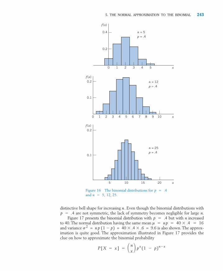
distinctive bell shape for increasing n . Even though the binomial distributions withare not symmetric, the lack of symmetry becomes negligible for large n.
Figure 17 presents the binomial distribution with but with n increasedto 40.The normal distribution having the same mean and variance = n p (1 � p) = 40 .4 .6 = 9.6 is also shown. The approx-imation is quite good. The approximation illustrated in Figure 17 provides theclue on how to approximate the binomial probability
P [ X � x ] � � nx
� p x ( 1 � p )
n � x
� 2
µ � n p � 40 .4 � 16p � .4
p � .4
5. THE NORMAL APPROXIMATION TO THE BINOMIAL 243
0.4 n = 5p = .4
n = 12p = .4
0.2
0.2
0.1
0 1 2 3 4 5 x
0 1 2 3 4 5 6 7 8 9 10 x
n = 25p = .4
0.2
0.1
105 15 20 x
f (x)
f (x)
f (x)
Figure 16 The binomial distributions for and 12, 25.n � 5,
p � .4
c06.qxd 10/15/09 11:06 AM Page 243

by a normal probability. The normal probability assigned to a single value x iszero. However, as shown in Figure 18, the probability assigned to the interval
to is the appropriate comparison. The addition and subtraction of is called the continuity correction.
The idea of the continuity correction is to approximate the rectangle with
area by the area under a normal curve. For and
the binomial distribution assigns
Recall from Chapter 5 that the binomial distribution has
To obtain an approximation, we select the normal distribution with the samemean, m � 6, and same s � 1.897. The normal approximation is then theprobability assigned to the interval to 7 � 1
2 .7 � 12
sd � √ n p ( 1 � p ) � √ 15 ( .4 )( .6 ) � 1.897
Mean � n p � 15 ( .4 ) � 6
P [ X � 7 ] � .787 � .610 � .177
p � .4,
n � 15� n x � p
x( 1 � p )n � x
12
x � 12x � 1
2
244 CHAPTER 6/THE NORMAL DISTRIBUTION
Figure 18 Idea of continuity correction.
–x 12
x
+x 12
Figure 17 The binomial distribution for p = .4 and n = 40 along with the normal densityhaving the same mean 16 and standard deviation 3.10.
0 3 6 9 12 15 18 21 24 27 30 33 36 39
X
0.12
0.08
0.04
Pro
babi
lity
c06.qxd 10/15/09 11:06 AM Page 244

Of course is small, so the approximation .1814 differs somewhat fromthe exact value .177. However, the accuracy of the approximation increaseswith the number of trials n.
The normal approximation to the binomial applies when n is large and the successprobability p is not too close to 0 or 1.The binomial probability of isapproximated by the normal probability of [ a � 1
2 � X � b � 12
] .[ a � X � b ]
n � 15
� P [ .264 � Z � .791 ] � .7855 � .6041 � .1814
P [ 6.5 � X � 7.5] � P �
6.5 � 61.897
�X � 61.897
�7.5 � 6
1.897 �
5. THE NORMAL APPROXIMATION TO THE BINOMIAL 245
The Normal Approximation to the Binomial
When np and n (1 � p ) are both large, say, greater than 15, the binomialdistribution is well approximated by the normal distribution having mean � np and sd � That is,
Z �X � n p
√ n p (1 � p ) is approximately N ( 0, 1 )
√ n p ( 1 � p ).
3
3To be consistent with the rule in Chapter 13 some suggest using the normal approximation when np isgreater than 5. The exact calculation of binomial probabilities using statistical software is always preferable.
Example 9 Normal Approximation to the BinomialIn a large scale statewide survey concerning television viewing by children,about 40% of the babies a few months old were reported to watch TV regu-larly. In a future random sample of 150 babies in this age group, let X be thenumber who regularly watch TV. Approximate the probability that
(a) X is between 52 and 71 both inclusive.
(b) X is greater than 67.
SOLUTION (a) Because the population is large, X has a binomial distribution with p = .4.To obtain a normal approximation, we first calculate the mean and stan-dard deviation of X. Since
The standardized variable is
The event includes both endpoints. The appropriate con-tinuity correction is to subtract from the lower end and add to the upperend. We then approximate
12
12
[52 � X � 71]
Z �X � 60
6
sd � √ n p ( 1 � p ) � √ 150 ( .4 )( .6 ) � √ 36 � 6
Mean � n p � 150 ( .4 ) � 60
n � 150,
c06.qxd 10/15/09 11:06 AM Page 245

where Z is standard normal. From the normal table, we interpolate
and approximate by the normal probability .8942.(b) For we reason that 67 is not included so that
or is the event of interest:
The normal approximation to the binomial gives
Example 10 A Normal Probability Approximation for a SurveyA recent study reported that 54% of the adults in the United States drink atleast one cup of coffee a day. If this is still the current rate, what is the proba-bility that in a random sample of 1000 adults the number that drink at leastone cup of coffee a day will be (a) less than 519 and (b) 556 or more?
SOLUTION Let X be the number of adults in the sample of 1000 adults who drink atleast one cup of coffee a day. Under the assumption that the proportion re-mains at .54, the distribution of X is well modeled by the binomial distribu-tion with n = 1000 and p = .54. Since n is large and
the binomial distribution of X is approximately N ( 540, 15.76 ).
(a) Because X is a count, the event [X < 519] is the same as [X � 518].Using the continuity correction, we have
(b)
Remark: If the object is to calculate binomial probabilities, today thebest practice is to evaluate them directly using an established statistical
� 1 � .8373 � .1627
� P [ Z � .9835]
P [X � 556] � P �Z �555.5 � 540
15.76 �
� .0863
� P [Z � �1.364]
P [ X � 518] � P �Z �518.5 � 540
15.76 �
n p � 540, √ n p ( 1 � p ) � √ 284.4 � 15.76
P [ X � 67] � .1056.
� P [ Z � 1.25 ] � 1 � .8944
P [ X � 67.5] � P �
X � 606
�67.5 � 60
6 �
[ X � 67.5 ][ X � 67 � .5 ][ X � 67 ] ,
P [ 52 � X � 71 ]
P [�1.417 � Z � 1.917 ] � .9724 � .0782 � .8942
� P [�1.417 � Z � 1.917]
P [ 51.5 � X � 71.5 ] � P �
51.5 � 606
�X � 60
6�
71.5 � 606
�
246 CHAPTER 6/THE NORMAL DISTRIBUTION
c06.qxd 10/15/09 11:06 AM Page 246
6.39 Let the number of successes X have a binomialdistribution with and (a) Find the exact probabilities of each of the
following:
X � 17 11 � X � 18 11 � X � 18
(b) Apply the normal approximation to eachsituation in part (a).
6.40 Let the number of successes X have a binomialdistribution with and
(a) Find the exact probability of each of thefollowing:
X � 11 6 � X � 12 6 � X � 12
(b) Apply the normal approximation to eachsituation in part (a).
6.41 A survey by the National Endowment of the Artsconcerned participation in music, plays, or danceperformance. About 17% of persons 18–24 yearsold participated in the last 12 months. Supposeyou will randomly select n = 300 persons in thisage group. Let success correspond to participationand let X denote the number of successes.Approximate the probability of (a) X = 60 (b) X � 45 and (c) 48 � X � 69
6.42 A National Newspaper Association survey showedthat 66% of adults would prefer to get their localnews and information from a local paper. Supposeyou will randomly select n = 200 adults. Let suc-cess correspond to prefer local paper and let X de-note the number of successes. Use the normal dis-tribution to approximate the probability of
(a)
(b)
(c) 137 � X � 152
X � 150
X � 130
p � .4.n � 25
p � .6.n � 25
5. THE NORMAL APPROXIMATION TO THE BINOMIAL 247
6.43 State whether or not the normal approximationto the binomial is appropriate in each of the fol-lowing situations.(a)
(b)
(c)
(d)
6.44 State whether or not the normal approximationto the binomial is appropriate in each of the fol-lowing situations.(a)
(b)
(c)
(d)
(e)
6.45 Copy Figure 16 and add the standard score scaleunderneath the
x-axis for 12, 25. Notice how the distributions center on zero and most of theprobability lies between and
6.46 The median age of residents of the United Statesis 35.6 years. If a survey of 200 residents istaken, approximate the probability that at least110 will be under 35.6 years of age.
6.47 The unemployment rate in a city is 7.9%. Asample of 300 persons is selected from the laborforce. Approximate the probability that(a) Less than 18 unemployed persons are in
the sample(b) More than 30 unemployed persons are in
the sample
z � 2.z � �2
n � 5,√ n p ( 1 � p )z � ( x � n p ) /
p � .71n � 100,
p � .97n � 150,
p � .02n � 300,
p � .40n � 10,
p � .23n � 500,
p � .40n � 61,
p � .98n � 120,
p � .03n � 100,
p � .24n � 90,
computing package. The numerical details need not concern us. However,the fact that
is approximately normal
when np and are both large remains important. We will use it in laterchapters when discussing inferences about proportions. Because the continuity correc-tion will not be crucial, we will drop it for the sake of simplicity. Beyond this chapter,we will employ the normal approximation but without the continuity correction.
Exercises
n ( 1 � p )
X � n p
√ n p ( 1 � p )
c06.qxd 10/15/09 11:06 AM Page 247

*6. CHECKING THE PLAUSIBILITY OF A NORMAL MODEL
Does a normal distribution serve as a reasonable model for the population thatproduced the sample? One reason for our interest in this question is that manycommonly used statistical procedures require the population to be nearly nor-mal. If a normal distribution is tentatively assumed to be a plausible model, theinvestigator must still check this assumption once the sample data are obtained.
Although they involve subjective judgment, graphical procedures prove mosthelpful in detecting serious departures from normality. Histograms can be inspectedfor lack of symmetry. The thickness of the tails can be checked for conformancewith the normal by comparing the proportions of observations in the intervals
and with thosesuggested by the empirical guidelines for the bell-shaped (normal) distribution.
A more effective way to check the plausibility of a normal model is to con-struct a special graph, called a normal-scores plot, of the sample data. In order todescribe this method, we will first explain the meaning of normal scores, indicatehow the plot is constructed, and then explain how to interpret the plot. For an easyexplanation of the ideas, we work with a small sample size. In practical applications,at least 15 or 20 observations are needed to detect a meaningful pattern in the plot.
The term normal scores refers to an idealized sample from the standard normaldistribution—namely, the z values that divide the standard normal distribution into
x � 3 s )( x � 3 s ,x � 2 s ) ,( x � 2 s ,( x � s , x � s ) ,
248 CHAPTER 6/THE NORMAL DISTRIBUTION
6.48 A survey reports that 96% of the people thinkthat violence has increased in the past five years. Out of a random sample of 50 persons,48 expressed the opinion that citizens have become more violent in the past five years. Doesthe normal approximation seem appropriate for the number of persons who ex-pressed the opinion that citizens have be-come more violent in the past five years? Explain.
6.49 According to the U. S. Statistical Abstract 2009,about 25% of persons age 18–24 participated incharity work in the past year. Among a sample of64 persons in this age group, find the probabilitythat 20 or more participated in charity work.
6.50 The weekly amount spent by a small companyfor in-state travel has approximately a normaldistribution with mean $1450 and standard de-viation $220. What is the probability that theactual expenses will exceed $1560 in 20 ormore weeks during the next year?
6.51 With reference to Exercise 6.50, calculate theprobability that the actual expenses would ex-ceed $1500 for between 18 and 24 weeks, inclu-sive during the next year.
X �
6.52 In a large midwestern university, 30% of the stu-dents live in apartments. If 200 students are ran-domly selected, find the probability that thenumber of them living in apartments will be be-tween 55 and 70 inclusive.
6.53 According to a study of mobility, 33% of U.S.residents in the age group 20 to 24 years movedto different housing in 2002 from where theylived in 2001. (Based on Statistical Abstract of theU.S. 2003, Table 34.) If the same percentageholds today, give the approximate probabilitythat in a random sample of 100 residents 20 to24 years old, there will be 39 or more personswho have moved in the past year.
6.54 Suppose that 20% of the trees in a forest are in-fested with a certain type of parasite.(a) What is the probability that, in a random
sample of 300 trees, the number of treeshaving the parasite will be between 49 and71 inclusive?
*(b) After sampling 300 trees, suppose that 72 treesare found to have the parasite. Does this pro-vide strong evidence that the population pro-portion is higher than 20%? Base your answeron when 20% are infested.P [ X � 72 ]
c06.qxd 10/15/09 11:06 AM Page 248

equal-probability intervals. For purposes of discussion, suppose the sample size isFigure 19 shows the standard normal distribution where four points are lo-
cated on the z axis so the distribution is divided into five segments of equal proba-bility These four points, denoted by , , , and , are precisely thenormal scores for a sample of size Using Appendix B, Table 3, we find that
A normal-scores plot allows us to visually assess how well a sample mimics theidealized normal sample. To construct a normal-scores plot:
1. Order the sample data from smallest to largest.2. Obtain the normal scores.3. Pair the ith largest observation with the ith largest normal score and
plot the pairs in a graph.
Example 11 Making a Normal-Scores Plot for Sample Size 4Suppose a random sample of size 4 has produced the observations 68, 82, 44,and 75. Construct a normal-scores plot.
SOLUTION The ordered observations and the normal scores are shown in Table 2, andthe normal-scores plot of the data is given in Figure 20.
m4 � .84m3 � .25m2 � �.25m1 � �.84
n � 4.m
4m 3m
2m115 � .2.
n � 4.
6. CHECKING THE PLAUSIBILITY OF A NORMAL MODEL 249
.2 .2m1 m2 m3 m4 z
.2 .2 .2
Figure 19 The N (0, 1) distribution and the normal scores for .n � 4
40
50
60
70
80
Ord
ered
obs
erva
tion
s
–1 0 1
Normal scores
TABLE 2 Normal Scores
OrderedNormal Scores Sample
� �.84 44� �.25 68� .25 75� .84 82m
4
m 3
m 2
m 1
Figure 20 Normal-scores plot of Table 2data.
c06.qxd 10/15/09 11:06 AM Page 249

INTERPRETATION OF THE PLOT
How does the normal-scores plot of a data set help in checking normality? Toexplain the main idea, we continue our discussion with the data of Example 11.Let m and s denote the mean and standard deviation of the population fromwhich the sample was obtained. The normal scores that are the idealized zobservations can then be converted to the x scale by the usual relation x �m � sz. The actual x observations and the corresponding idealized observations are given in Table 3. If the population were indeed normal, we would expect the two columns of Table 3 to be close. In other words, a plot of the observed x values versus the normal scores would produce a straight-line pattern, wherethe intercept of the line would indicate the value of m and the slope of the linewould indicate s.
250 CHAPTER 6/THE NORMAL DISTRIBUTION
TABLE 3 Idealized Sample
Observed Idealizedx Values x Values
44 m � s
68 m � s
75 m � s
82 m � s m 4
m 3
m 2
m 1
A straight line pattern in a normal-scores plot supports the plausibility ofa normal model. A curve appearance indicates a departure from normality.
A normal-scores plot is easily obtained using software packages. The nextexample illustrates a straight-line pattern consistent with the assumption thatthe population is normal.
Example 12 A Normal Scores Plot That Looks NormalConsider the data on the growth of salmon in Table D.7 of the Data Bank.We plot the freshwater growth of female salmon measured in terms of widthof growth rings in hundredths of an inch. Create a normal-scores plot ofthese data and comment on the pattern.
SOLUTION We use MINITAB software as described in Exercise 6.80 to make the normalscores plot in Figure 21.
c06.qxd 10/15/09 11:06 AM Page 250

7. TRANSFORMING OBSERVATIONS TO ATTAIN NEAR NORMALITY 251
125
150
175
100
75
50
–2 –1 0
Normal score
1 2
Fres
hwat
er g
row
th (
.01
in)
Notice that the plot conforms quite well to the straight-line pattern ex-pected for normal observations. The assumption of a normal distributionseems quite reasonable.
The MINITAB package that produced Figure 21 uses one of the manyslight variants of the normal scores above but the plots are similar if the sam-ple size is greater than 20.
*7. TRANSFORMING OBSERVATIONS TO ATTAIN NEAR NORMALITY
A valid application of many powerful techniques of statistical inference, espe-cially those suited to small or moderate samples, requires that the populationdistribution be reasonably close to normal. When the sample measurements ap-pear to have been taken from a population that departs drastically from normal-ity, an appropriate conversion to a new variable may bring the distribution closeto normal. Efficient techniques can then be safely applied to the converted data,whereas their application to the original data would have been questionable. In-ferential methods requiring the assumption of normality are discussed in laterchapters. The goal of our discussion here is to show how a transformation canimprove the approximation to a normal distribution.
There is no rule for determining the best transformation in a given situa-tion. For any data set that does not have a symmetric histogram, we consider avariety of transformations.
Figure 21 A normal-scores plot of the female salmon growth infreshwater.
c06.qxd 10/15/09 11:06 AM Page 251

252 CHAPTER 6/THE NORMAL DISTRIBUTION
TABLE 4 Volume of Timber in Cords
39.3 14.8 6.3 .9 6.53.5 8.3 10.0 1.3 7.16.0 17.1 16.8 .7 7.92.7 26.2 24.3 17.7 3.27.4 6.6 5.2 8.3 5.93.5 8.3 44.8 8.3 13.4
19.4 19.0 14.1 1.9 12.019.7 10.3 3.4 16.7 4.31.0 7.6 28.3 26.2 31.78.7 18.9 3.4 10.0
Courtesy of Professor Alan Ek.
You may recall that x is the natural logarithm. Fortunately, computerseasily calculate and order the transformed values, so that several transformationsin a list can be quickly tested. Note, however, that the observations must be pos-itive if we intend to use and x .
The selection of a good transformation is largely a matter of trial and error.If the data set contains a few numbers that appear to be detached far to the right, and x , or negative powers that would pull these stragglerscloser to the other data points should be considered.
Example 13 A Transformation to Improve NormalityA forester records the volume of timber, measured in cords, for 49 plots se-lected in a large forest. The data are given in Table 4 and the correspondinghistogram appears in Figure 22a. The histogram exhibits a long tail to the right, so it is reasonable to consider the transformations x , and1/x. Transform the data to near normality.
SOLUTION The most satisfactory result, obtained with
is illustrated in Table 5 and Figure 22b. The latter histogram more nearly re-sembles a symmetric bell-shaped pattern expected for normal populations.
Transformed data � √4 Volume
loge√4 x ,√x ,
loge√4 x ,√x ,
loge√4 x ,√x ,
loge
Some Useful Transformations
Make large values larger: Make large values smaller:
, x ,1x
loge√4 x ,√x ,x
2x
3
c06.qxd 10/15/09 11:06 AM Page 252

7. TRANSFORMING OBSERVATIONS TO ATTAIN NEAR NORMALITY 253
TABLE 5 The Transformed Data
2.50 1.96 1.58 .97 1.601.37 1.70 1.78 1.07 1.631.57 2.03 2.02 .91 1.681.28 2.26 2.22 2.05 1.341.64 1.60 1.51 1.70 1.561.37 1.70 2.59 1.70 1.912.10 2.09 1.94 1.17 1.862.11 1.79 1.36 2.02 1.441.00 1.66 2.31 2.26 2.371.72 2.09 1.36 1.78
√4 Volume
Figure 22 An illustration of the transformation technique. (a) Histogram of timber volume.
(b) Histogram of .4√ Volume
0
.05
10 20 30
Volume (in cords)
40 50
(a)
0
.5
1.0
0.5 1.0 2.01.54
Volume
2.5 3.0
(b)
c06.qxd 10/15/09 11:06 AM Page 253

254 CHAPTER 6/THE NORMAL DISTRIBUTION
USING STATISTICS WISELY
1. A sketch of the bell-shaped normal curve and the area of interest canprevent blunders when determining probabilities and percentiles.
2. Never apply the normal approximation to the binomial, treating
as standard normal, when the expected number of successes (or fail-ures) is too small. That is, when either
3. Do not just assume that data come from a normal distribution. Whenthere are at least 20 to 25 observations, it is good practice to construct anormal-scores plot to check this assumption.
n p or n ( 1 � p ) is 15 or less
Z �X � n p
√ n p ( 1 � p )
HOW MUCH TIMBER IS IN THIS FOREST?The volume of timber available for making lumber can only be estimated by samplingthe number of trees in randomly selected plots within the forest. The distribution oftree size must also be taken into account. © Anthony Baggett/Stockphoto.
c06.qxd 10/15/09 11:06 AM Page 254

KEY IDEAS AND FORMULAS
The probability distribution for a continuous random variable X is specifiedby a probability density curve. The function that specifies this curve iscalled a probability density function. It can be symmetric about the mean ofX or it can be skewed, meaning that it has a long tail to either the left or theright.
The probability that X lies in an interval from a to b is determined by thearea under the probability density curve between a and b. The total area underthe curve is 1, and the curve is never negative.
The population 100 p-th percentile is an x value that has probability p to itsleft and probability 1 – p to its right.
When X has mean m and standard deviation s, the standardized variable
has mean 0 and standard deviation 1.The normal distribution has a symmetric bell-shaped curve centered at the
mean. The intervals extending one, two, and three standard deviations aroundthe mean contain the probabilities .683, .954, and .997, respectively.
If X is normally distributed with mean m and standard deviation s, then
has the standard normal distribution.When the number of trials n is large and the success probability p is not too
near 0 or 1, the binomial distribution is well approximated by a normal distribu-tion with mean np and sd � Specifically, the probabilities for abinomial variable X can be approximately calculated by treating
as standard normal. For a moderate number of trials n, the approximation is im-proved by appropriately adjusting by called a continuity correction.
The normal scores are an ideal sample from a standard normal distribution.Plotting each ordered observation versus the corresponding normal score createsa normal-scores plot, which provides a visual check for possible departures froma normal distribution.
Transformation of the measurement scale often helps to convert a long-tailed distribution to one that resembles a normal distribution.
12
Z �X � np
√ n p ( 1 � p )
√ n p ( 1 � p ) .
Z �X � �
�
Z �X � m
s
KEY IDEAS AND FORMULAS 255
c06.qxd 10/15/09 11:06 AM Page 255

256 CHAPTER 6/THE NORMAL DISTRIBUTION
TECHNOLOGY
Probability and Percentiles for the Standard Normal and General Normal Distribution
MINITAB
MINITAB uses the same steps for calculations with the standard normal andcases of other means and standard deviations. We illustrate with the calcula-tion of when X is normal with mean 5 and standard deviation12.5.
Calc > Probability Distributions > Normal.Select Cumulative Probability. Type 5 in Mean.Type 12.5 in Standard deviation.Select Input Constant and type 8. Click OK.
The default settings Mean 0 and Standard deviation 1 simplify the steps for ob-taining standard normal probabilities.
The inverse problem of finding b so that where a is aspecified probability, is illustrated with finding b so that when X is normal with mean 5 and standard deviation 12.5.
Calc > Probability Distributions > Normal.Select Inverse Probability. Type 5 in Mean.Type 12.5 in Standard deviation.Select Input Constant and type .9700. Click OK.
EXCEL
EXCEL uses the function NORMSDIST for standard normal probabilities andNORMDIST for a general normal distribution. We illustrate with the calculationof when X is normal with mean 5 and standard deviation 12.5.
Select the icon, or select Insert and then Function.Choose Statistical and then NORMDIST. Click OK.Type 8 in X, 5 in Mean, 12.5 in Standard_dev and True in Cumulative.Click OK.
The inverse problem of finding b so that where a is a speci-fied probability, is illustrated with finding b so that whenX is normal with mean 5 and standard deviation 12.5.
Select the icon, or select Insert and then Function.Choose Statistical, and then NORMINV. Click OK.Type .9700 in Probability, 5 in Mean, 12.5 in Standard_dev. Click OK.
fx
P [X � b ] � .9700P [X � b ] � a,
fx
P [X � 8 ]
P [X � b ] � .9700P [ X � b ] � a ,
P [X � 8 ]
c06.qxd 10/15/09 11:06 AM Page 256

6.55 Determine (a) the median and (b) the quartilesfor the distribution shown in the following illus-tration.
6.56 For X having the density in Exercise 6.55, find(a) (b) and(c)
6.57 In the context of the height of red pine seedlingspresented at the front of the chapter, describethe reasoning that leads from a histogram to theconcept of a probability density curve. (Think ofsuccessive histograms based on 100 heights, 500
P [ .5 � X � .7 ].P [ .5 � X � .7 ]P [ X � .7 ]
8. REVIEW EXERCISES 257
heights, 1456 heights, and then an unlimitednumber.)
6.58 For a standard normal random variable Z, find
(a)
(b)
(c)
(d)
6.59 For the standard normal distribution, find thevalue z such that
(a) Area to its left is .0838
(b) Area to its left is .047
(c) Area to its right is .2611
(d) Area to its right is .12
6.60 Find the 20th, 40th, 60th, and 80th percentilesof the standard normal distribution.
P [ �1.47 � Z � 1.055]
P [ .61 � Z � 1.92]
P [ Z � 1.245 ]
P [ Z � 1.26 ]
x
1
0 1
f (x)
8. REVIEW EXERCISES
To solve the standard normal inverse problem replace NORMINV by NORM-SINV.
TI-84/-83 PLUS
We illustrate with the calculation of when X is normal withmean 5 and standard deviation 12.5.
In the Home screen, press VARS
From the DISTR menu, select 2: Normalcdf(.
Type entries to obtain Normalcdf ( —1E99, 8, 5, 12.5 ),Then press ENTER.
The inverse problem of finding b so that where a is a speci-fied probability, is illustrated with finding b so that whenX is normal with mean 5 and standard deviation 12.5.
In the Home screen, press VARS.From the DISTR mean, select 3: InvNorm(.Type entries to obtain InvNorm( .9700, 5, 12.5).Then press ENTER.
2nd
P [ X � b ] � .9700P [ X � b ] � a,
2nd
P [ X � 8 ]
c06.qxd 10/15/09 11:06 AM Page 257

6.61 If Z is a standard normal random variable, whatis the probability that
(a) Z exceeds .62?
(b) Z lies in the interval (�1.40, 1.40)?
(c) exceeds 3.0?
(d) is less than 2.0?
6.62 According to Example 12, a normal distributionwith mean 115 and standard deviation 22 hun-dredths of an inch describes variation in femalesalmon growth in fresh water.
(a) If a newly caught female salmon has growth108, what is the corresponding standard-ized score?
(b) If a standardized score is �.8, what is thegrowth measurement?
(c) Find the interval of standardized scorescorresponding to the growth measurements105 to 128.
(d) Find the interval of growth measurementscorresponding to the standardized scores of�1.5 to 1.5.
6.63 The bell-shaped histogram for the heights ofthree-year-old red pine seedlings on page 222 isconsistent with the assumption of a normal distrib-ution having mean = 280 and sd = 58 millimeters.Let X denote the height, at three years of age, ofthe next red pine that will be measured. Find
(a)
(b)
(c)
(d)
(e)
(f)
6.64 If X has a normal distribution with m � 100and s � 5, find b such that
(a)
(b)
(c)
6.65 Suppose that a student’s verbal score X from nextyear’s Graduate Record Exam can be consideredan observation from a normal population havingmean 499 and standard deviation 120. Find
(a) P [ X � 600 ]
P [ � X � 100 � � b ] � .966
P [ X � b ] � .0110
P [ X � b ] � .6700
P [305 � X � 405]
P [235 � X � 335]
P [ X � 90]
P [ X � 230]
P [ X � 240]
P [ X � 337]
� Z �� Z �
258 CHAPTER 6/THE NORMAL DISTRIBUTION
(b) 90th percentile of the distribution
(c) Probability that the student scores below400
6.66 The lifting capacities of a class of industrial work-ers are normally distributed with mean 65 poundsand standard deviation 8 pounds. What propor-tion of these workers can lift an 80-pound load?
6.67 The bonding strength of a drop of plastic glue isnormally distributed with mean 100 poundsand standard deviation 8 pounds. A broken plas-tic strip is repaired with a drop of this glue andthen subjected to a test load of 90 pounds.What is the probability that the bonding willfail?
6.68 Grading on a curve. The scores on an ex-amination are normally distributed with mean m� 70 and standard deviation s � 8. Supposethat the instructor decides to assign letter gradesaccording to the following scheme ( left end-point included).
Find the percentage of students in each gradecategory.
6.69 Suppose the duration of trouble-free operationof a new robotic vacuum cleaner is normally dis-tributed with mean 750 days and standard devi-ation 100 days.
(a) What is the probability that the vacuumcleaner will work for at least two yearswithout trouble?
(b) The company wishes to set the warrantyperiod so that no more than 10% of thevacuum cleaners would need repair ser-vices while under warranty. How long awarranty period must be set?
6.70 Suppose the amount of a popular sport drink inbottles leaving the filling machine has a normal
Scores Grade
Less than 58 F58 to 66 D66 to 74 C74 to 82 B82 and above A
c06.qxd 10/15/09 11:06 AM Page 258

distribution with mean 101.5 milliliters (ml)and standard deviation 1.6 ml.
(a) If the bottles are labeled 100 ml, what pro-portion of the bottles contain less than thelabeled amount.
(b) If only 5% of the bottles have contents thatexceed a specified amount v, what is thevalue of v?
6.71 Suppose the amount of sun block lotion in plas-tic bottles leaving a filling machine has a normaldistribution. The bottles are labeled 300 milli-liters (ml) but the actual mean is 302 ml andthe standard deviation is 2 ml.
(a) What is the probability that an individualbottle will contain less than 299 ml?
(b) If only 5% of the bottles have contents thatexceed a specified amount v, what is thevalue of v?
*6.72 A property of the normal distribution. Supposethe random variable X is normally distributedwith mean m and standard deviation s. If Y is alinear function of X—that is, Y � a � bX,where a and b are constants—then Y is also nor-mally distributed with
For instance, if X is distributed as N ( 25, 2) andY � 7 � 3X, then the distribution of Y is normal with Mean � 7 � 3(25) � �68 and sd �
(a) At the “low” setting of a water heater, thetemperature X of water is normally dis-tributed with Mean � 102°F and sd �4°F. If Y refers to the temperature mea-surement in the centigrade scale, that is,Y � what is the distributionof Y?
(b) Referring to part (a), find the probability of[35 � Y � 42].
Remark: The relation between a general normaland the standard normal is only a special case ofthis property. Specifically, the standardized vari-able Z is the linear function.
59 ( X � 32 ) ,
� �3 � 2 � 6.
sd � � b ��
Mean � a � b�
8. REVIEW EXERCISES 259
where Z has
6.73 Let X denote the number of successes in nBernoulli trials with a success probability of p.
(a) Find the exact probabilities of each of thefollowing:
(i) X � 7 when
(ii) 11 � X � 16 when
(iii) X � 9 when
(b) Use a normal approximation for each situa-tion in part (a).
6.74 It is known from past experience that 7% of thetax bills are paid late. If 20,000 tax bills are sentout, find the probability that:
(a) Less than 1350 are paid late.
(b) 1480 or more are paid late.
6.75 A particular program, say, program A, previouslydrew 30% of the television audience. To deter-mine if a recent rescheduling of the programs ona competing channel has adversely affected theaudience of program A, a random sample of 400viewers is to be asked whether or not they cur-rently watch this program.
(a) If the percentage of viewers watching pro-gram A has not changed, what is the proba-bility that fewer than 103 out of a sampleof 400 will be found to watch the program?
(b) If the number of viewers of the program isactually found to be less than 103, will thisstrongly support the suspicion that thepopulation percentage has dropped? Useyour calculation from part (a).
6.76 The number of successes X has a binomial dis-tribution. State whether or not the normal
n � 16, p � .5
n � 20, p � .7
n � 25, p � .4
sd �1
� � � 1
Mean � �
�
��
1
� � � 0
Z �X � �
�� �
�
��
1
� X
c06.qxd 10/15/09 11:06 AM Page 259

260 CHAPTER 6/THE NORMAL DISTRIBUTION
approximation is appropriate in each of the fol-lowing situations: (a) (b)
(c)
6.77 Because 10% of the reservation holders are “no-shows,” a U.S. airline sells 400 tickets for a flightthat can accommodate 370 passengers.
(a) Find the probability that one or morereservation holders will not be accommo-dated on the flight.
(b) Find the probability of fewer than 350 pas-sengers on the flight.
6.78 On a Saturday afternoon, 147 customers will beobserved during check-out and the number payingby card, credit or debit, will be recorded. Recordsfrom the store suggest that 43% of customers payby card.Approximate the probability that:
(a) More than 60 will pay by card.
(b) Between 60 and 70, inclusive, will pay bycard.
6.79 In all of William Shakespeare’s works, heused different words. Of these,14,376 appeared only once. In 1985 a 429-word poem was discovered that may havebeen written by Shakespeare. To keep theprobability calculations simple, assume thatthe choices between a new word and onefrom the list of 884,647 are independent foreach of the 429 words. Approximate theprobability that a new word will not be onthe list, by the relative frequency of wordsused once.
(a) Find the expected number of new words inthe poem.
(b) Use the normal approximation to the bino-mial to determine the probability of finding12 or more new words in the poem. Usethe continuity correction.
(c) Use the normal approximation to the bino-mial to determine the probability of finding2 or fewer new words in the poem. Use thecontinuity correction.
884,6474
n � 90, p � .98.n � 20, p � .03n � 400, p � .23
Calc > Calculator.
Type C2 in Store. Type NSCOR(C1) in Expres-sion. Click OK.
Graph > Scatterplot. Select Simple. Type C1 un-der Y variables and C2 under X variables. ClickOK.
will create a normal-scores plot for the observa-tions in C1. ( MINITAB uses a variant of thenormal scores, , that we defined )
*6.81 Use MINITAB or another package program tomake a normal-scores plot of the malt extractdata in Table D.8 of the Data Bank.
*6.82 Use MINITAB or another package program tomake a normal-scores plot of the computer anx-iety scores in Table D.4 of the Data Bank.
mi
See R. Thisted and B. Efron. “Did Shakespeare write a newly-discovered poem?” Biometrika, 74, (1987) pp. 445–455.
4
(d) Use the normal approximation to the bino-mial to determine the probability of findingmore than 2 but less than 12 new words inthe poem. On the basis of your answer, de-cide if 9 � actual number of new wordsnot in the list is consistent with Shake-speare having written the poem or if it con-tradicts this claim.
The Following Exercises Require a Computer
6.80 Normal-scores plot. Use a computer programto make a normal-scores plot for the volume oftimber data in Table 4. Comment on the depar-ture from normality displayed by the normal-scores plot.
We illustrate a normal-scores plot usingMINITAB. With the data set in column 1, theMINITAB commands
c06.qxd 10/15/09 11:06 AM Page 260

will place the natural logarithm x in C2,in C3, and in C4. Normal-scores plots canthen be constructed as in Exercise 6.80.
Refer to the lightning data in Exercise 2.121 ofChapter 2. Make a normal-scores plot of the
(a) original observations.
(b) fourth root of the original observations.
(c) Comment on the quality of the approxima-tion by a normal distribution in both cases.
x1/4√xloge
8. REVIEW EXERCISES 261
Dialog box:
Calc > Calculator. Type C2 in Store. TypeLOGE(C1) in Expression. Click OK.
Calc > Calculator. Type C3 in Store. TypeSQRT(C1) in Expression. Click OK.
Calc > Calculator. Type C4 in Store. TypeSQRT(C2) in Expression. Click OK.
*6.83 Transformations and normal-scores plots.The MINITAB computer language makes it pos-sible to easily transform data. With the data al-ready set in column 1, the commands
c06.qxd 10/15/09 11:06 AM Page 261

c06.qxd 10/15/09 11:06 AM Page 262
1. Introduction2. The Sampling Distribution of a Statistic3. Distribution of the Sample Mean and
the Central Limit Theorem4. Statistics in Context5. Review Exercises
7
Variation in Repeated Samples —Sampling Distributions
c07.qxd 10/15/09 11:07 AM Page 263

Bowling AveragesA bowler records individual game scores and the average for a three-game series.
100 125 150 175 200 225
Average
Game 1
100 125 150 175 200 225
Bowlers are well aware that their three-game averages are less variable than their single-game scores.Sample means always have less variability than individual observations. Spike Mafford/Alamy.
c07.qxd 10/15/09 11:07 AM Page 264

1. INTRODUCTION
At the heart of statistics lie the ideas of inference. They enable the investigatorto argue from the particular observations in a sample to the general case. Thesegeneralizations are founded on an understanding of the manner in which varia-tion in the population is transmitted, by sampling, to variation in statistics likethe sample mean. This key concept is the subject of this chapter.
Typically, we are interested in learning about some numerical feature of thepopulation, such as the proportion possessing a stated characteristic, the meanand standard deviation of the population, or some other numerical measure ofcenter or variability.
The true value of a population parameter is an unknown constant. It can becorrectly determined only by a complete study of the population. The conceptsof statistical inference come into play whenever this is impossible or not practi-cally feasible.
If we only have access to a sample from the population, our inferencesabout a parameter must then rest on an appropriate sample-based quantity.Whereas a parameter refers to some numerical characteristic of the population,a sample-based quantity is called a statistic.
For example, the sample mean
is a statistic because its numerical value can be computed once the sample data,consisting of the values of , . . . , , are available. Likewise, the sample me-dian and the sample standard deviation are also sample-based quantities so eachis a statistic. Note that every statistic is a random variable. A sample-based quan-tity (statistic) must serve as our source of information about the value of a para-meter. Three points are crucial:
1. Because a sample is only a part of the population, the numericalvalue of a statistic cannot be expected to give us the exact value ofthe parameter.
XnX1
X �X1 � ��� � Xn
n
1. INTRODUCTION 265
A numerical feature of a population is called a parameter.
A statistic is a numerical valued function of the sample observations.
c07.qxd 10/15/09 11:07 AM Page 265

2. The observed value of a statistic depends on the particular sample thathappens to be selected.
3. There will be some variability in the values of a statistic over differentoccasions of sampling.
A brief example will help illustrate these important points. Suppose an ur-ban planner wishes to study the average commuting distance of workers fromtheir home to their principal place of work. Here the statistical population con-sists of the commuting distances of all the workers in the city. The mean of thisfinite but vast and unrecorded set of numbers is called the population mean,which we denote by m . We want to learn about the parameter m by collectingdata from a sample of workers. Suppose 80 workers are randomly selected andthe (sample) mean of their commuting distances is found to be Evidently, the population mean m cannot be claimed to be exactly 8.3 miles. Ifone were to observe another random sample of 80 workers, would the samplemean again be 8.3 miles? Obviously, we do not expect the two results to beidentical. Because the commuting distances do vary in the population of work-ers, the sample mean would also vary on different occasions of sampling. Inpractice, we observe only one sample and correspondingly a single value of thesample mean such as However, it is the idea of the variability of the
values in repeated sampling that contains the clue to determining howprecisely we can hope to determine m from the information on
2. THE SAMPLING DISTRIBUTION OF A STATISTIC
The fact that the value of the sample mean, or any other statistic, will vary asthe sampling process is repeated is a key concept. Because any statistic, the sam-ple mean in particular, varies from sample to sample, it is a random variable andhas its own probability distribution. The variability of the statistic, in repeatedsampling, is described by this probability distribution.
The qualifier “sampling” indicates that the distribution is conceived in the con-text of repeated sampling from a population. We often drop the qualifier andsimply say the distribution of a statistic.
Although in any given situation, we are limited to one sample and the cor-responding single value for a statistic, over repeated samples from a populationthe statistic varies and has a sampling distribution. The sampling distribution ofa statistic is determined from the distribution f (x ) that governs the population,and it also depends on the sample size n. Let us see how the distribution of can be determined in a simple situation where the sample size is 2 and the pop-ulation consists of 3 units.
X
x.x
x � 8.3.
x � 8.3 miles.
266 CHAPTER 7/VARIATION IN REPEATED SAMPLES—SAMPLING DISTRIBUTIONS
The probability distribution of a statistic is called its sampling distribution.
c07.qxd 10/15/09 11:07 AM Page 266

Example 1 Illustration of a Sampling DistributionA population consists of three housing units, where the value of X, the num-ber of rooms for rent in each unit, is shown in the illustration.
Consider drawing a random sample of size 2 with replacement. That is,we select a unit at random, put it back, and then select another unit at random. Denote by and the observation of X obtained in the first and second drawing, respectively. Find the sampling distribution of
SOLUTION The population distribution of X is given in Table 1, which simply formalizesthe fact that each of the X values 2, 3, and 4 occurs in of the population ofthe housing units.
Because each unit is equally likely to be selected, the observation fromthe first drawing has the same distribution as given in Table 1. Since the samplingis with replacement, the second observation also has this same distribution.
The possible samples ( , ) of size 2 and the corresponding values of are
( , ) (2, 2) (2, 3) (2, 4) (3, 2) (3, 3) (3, 4) (4, 2) (4, 3) (4, 4)
2 2.5 3 2.5 3 3.5 3 3.5 4
The nine possible samples are equally likely so, for instance,Continuing in this manner, we obtain the distribution of
which is given in Table 2.X ,P [ X � 2.5 ] � 2
9 .
x �x1 � x2
2
x2x1
Xx2x1
X2
X1
13
X � ( X1 � X2 ) / 2.
X2X1
TABLE 1 The PopulationDistribution
x f (x )
2
3
413
13
13
2. THE SAMPLING DISTRIBUTION OF A STATISTIC 267
2 4 3
c07.qxd 10/15/09 11:07 AM Page 267

This sampling distribution pertains to repeated selection of randomsamples of size 2 with replacement. It tells us that if the random sampling isrepeated a large number of times, then in about , or 11%, of the cases, the sam-ple mean would be 2, and in , or 22%, of the cases, it would be 2.5, and so on.
Figure 1 shows the probability histograms of the distributions in Tables 1and 2.
In the context of Example 1, suppose instead the population consists of 300housing units, of which 100 units have 2 rooms, 100 units have 3 rooms, and100 units have 4 rooms for rent. When we sample two units from this large
29
19
268 CHAPTER 7/VARIATION IN REPEATED SAMPLES—SAMPLING DISTRIBUTIONS
2 3 4 x 2 3 4 x
1
3
1
3
1
3
1
9
2
9
3
9
2
9
1
9
TABLE 2 The Probability Distributionof ( � ) / 2
Value of Probability
2
2.5
3
3.5
419
29
39
29
19
X
X2X1X �
Figure 1 Idea of a sampling distribution.
(a) Population distribution.
( b) Sampling distributionof X � ( X1 � X2
) / 2.
c07.qxd 10/15/09 11:07 AM Page 268

More concisely, under the independence and same distribution conditions, werefer to the observations as a random sample.
Because of variation in the population, the random sample will vary and sowill the sample median, or any other statistic.
The next example further explores sampling distributions by focusing firston the role of independence in constructing a sampling distribution and thenemphasizing that this distribution too has a mean and variance.
Example 2 The Sample Mean and Median Each Have a Sampling DistributionA large population is described by the probability distribution
Let , , be a random sample of size 3 from this distribution.
(a) List all the possible samples and determine their probabilities.
(b) Determine the sampling distribution of the sample mean.
(c) Determine the sampling distribution of the sample median.
SOLUTION (a) Because we have a random sample, each of the three observations, , has the same distribution as the population and they are
independent. So, the sample 0, 3, 0 has probability ( .2 ) � (.3) �( .2) � 0.12. The calculations for all 3 � 3 � 3 � 27 possiblesamples are given in Table 3, page 270.
(b) The probabilities of all samples giving the same value are added toobtain the sampling distribution on the second page of Table 3.
(c) The calculations and sampling distribution of the median are alsogiven on the second page of Table 3.
x
X3X2X1
X3X2X1
X ,
population, it would make little difference whether or not we replace the unitafter the first selection. Each observation would still have the same probabil-ity distribution—namely,which characterizes the population.
When the population is very large and the sample size relatively small, it isinconsequential whether or not a unit is replaced before the next unit is se-lected. Under these conditions, too, we refer to the observations as a randomsample. What are the key conditions required for a sample to be random?
P [ X � 2 ] � P [ X � 3 ] � P [ X � 4 ] � 13 ,
2. THE SAMPLING DISTRIBUTION OF A STATISTIC 269
x f (x )
0 .23 .3
12 .5
The observations , , …, are a random sample of size n from thepopulation distribution if they result from independent selections andeach observation has the same distribution as the population.
XnX2X1
c07.qxd 10/15/09 11:07 AM Page 269

270 CHAPTER 7/VARIATION IN REPEATED SAMPLES—SAMPLING DISTRIBUTIONS
TABLE 3 Sampling Distributions
Population Distribution
� 27.09 � �2Population variance: Var ( X ) � 02 ( .2 ) � 32 ( .3 ) � 122 ( .5 ) � 6.92
Population mean: E ( X ) � 0 (.2 ) � 3 (.3 ) � 12 (.5 ) � 6.9 � �
Possible Sample SampleSamples Mean Median
m Probability
1 0 0 0 0 02 0 0 3 1 03 0 0 12 4 04 0 3 0 1 05 0 3 3 2 36 0 3 12 5 37 0 12 0 4 08 0 12 3 5 39 0 12 12 8 12
10 3 0 0 1 011 3 0 3 2 312 3 0 12 5 313 3 3 0 2 314 3 3 3 3 315 3 3 12 6 316 3 12 0 5 317 3 12 3 6 318 3 12 12 9 1219 12 0 0 4 020 12 0 3 5 321 12 0 12 8 1222 12 3 0 5 323 12 3 3 6 324 12 3 12 9 1225 12 12 0 8 1226 12 12 3 9 1227 12 12 12 12 12
Total � 1.000
(.5)(.5)(.5) � .125(.5)(.5)(.3) � .075(.5)(.5)(.2) � .050(.5)(.3)(.5) � .075(.5)(.3)(.3) � .045(.5)(.3)(.2) � .030(.5)(.2)(.5) � .050(.5)(.2)(.3) � .030(.5)(.2)(.2) � .020(.3)(.5)(.5) � .075(.3)(.5)(.3) � .045(.3)(.5)(.2) � .030(.3)(.3)(.5) � .045(.3)(.3)(.3) � .027(.3)(.3)(.2) � .018(.3)(.2)(.5) � .030(.3)(.2)(.3) � .018(.3)(.2)(.2) � .012(.2)(.5)(.5) � .050(.2)(.5)(.3) � .030(.2)(.5)(.2) � .020(.2)(.3)(.5) � .030(.2)(.3)(.3) � .018(.2)(.3)(.2) � .012(.2)(.2)(.5) � .020(.2)(.2)(.3) � .012(.2)(.2)(.2) � .008
xx3x2x1
x f (x )
0 .23 .3
12 .5
(Continued )
c07.qxd 10/15/09 11:07 AM Page 270
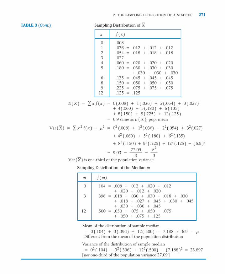
is one-third of the population variance.
Different from the mean of the population distribution
Variance of the distribution of sample median
[not one-third of the population variance 27.09]� 02 (.104) � 32 (.396) � 122(.500) � (7.188 )2 � 23.897
� 0 (.104) � 3(.396) � 12(.500) � 7.188 � 6.9 � �
Mean of the distribution of sample median
Var (X )
� 9.03 �27.09
3�
�2
3
� 82 ( .150 ) � 92(.225) � 122 (.125) � ( 6.9 )2
� 42 (.060) � 52 (.180) � 62 (.135)
Var ( X ) � � x 2 f ( x ) � �2 � 02 (.008) � 12 (.036) � 22 (.054) � 32 (.027)
� 6.9 same as E ( X ), pop. mean� 8 (.150 ) � 9 (.225 ) � 12 (.125 )� 4 ( .060) � 5 (.180 ) � 6 (.135)
E ( X ) � � x f (x ) � 0 ( .008 ) � 1 ( .036 ) � 2 ( .054 ) � 3 ( .027 )
2. THE SAMPLING DISTRIBUTION OF A STATISTIC 271
0 .0081 .036 � .012 � .012 � .0122 .054 � .018 � .018 � .0183 .0274 .060 � .020 � .020 � .0205 .180 � .030 � .030 � .030
� .030 � .030 � .0306 .135 � .045 � .045 � .0458 .150 � .050 � .050 � .0509 .225 � .075 � .075 � .075
12 .125 � .125
f ( x )x
TABLE 3 (Cont.) Sampling Distribution of X
m f (m)
0 .104 � .008 � .012 � .020 � .012� .020 � .012 � .020
3 .396 � .018 � .030 � .030 � .018 � .030� .018 � .027 � .045 � .030 � .045� .030 � .030 � .045
12 .500 � .050 � .075 � .050 � .075� .050 � .075 � .125
Sampling Distribution of the Median m
c07.qxd 10/15/09 11:07 AM Page 271

To illustrate the idea of a sampling distribution, we considered simple popu-lations with only three possible values and small sample sizes n � 2 and n �3. The calculation gets more tedious and extensive when a population has manyvalues of X and n is large. However, the procedure remains the same. Once thepopulation and sample size are specified:
1. List all possible samples of size n.
2. Calculate the value of the statistic for each sample.
3. List the distinct values of the statistic obtained in step 2. Calculate thecorresponding probabilities by identifying all the samples that yield thesame value of the statistic.
We leave the more complicated cases to statisticians who can sometimes use ad-ditional mathematical methods to derive exact sampling distributions.
Instead of a precise determination, one can turn to the computer in order toapproximate a sampling distribution. The idea is to program the computer toactually draw a random sample and calculate the statistic. This procedure is thenrepeated a large number of times and a relative frequency histogram con-structed from the values of the statistic. The resulting histogram will be an ap-proximation to the sampling distribution. This approximation will be used inExample 4.
Exercises
272 CHAPTER 7/VARIATION IN REPEATED SAMPLES—SAMPLING DISTRIBUTIONS
7.1 Identify each of the following as either a para-meter or a statistic.
(a) Sample standard deviation.
(b) Sample interquartile range.
(c) Population 20th percentile.
(d) Population first quartile.
(e) Sample median.
7.2 Identify the parameter, statistic, and populationwhen they appear in each of the following state-ments.
(a) During 2008, forty-one different moviesreceived the distinction of generating themost box office revenue for a weekend.
(b) A survey of 400 minority persons living inChicago revealed that 41 were out ofwork.
(c) Out of a sample of 100 dog owners whoapplied for dog licenses in northern Wis-consin, 18 had a Labrador retriever.
7.3 Data obtained from asking the wrong questionsat the wrong time or in the wrong place can leadto misleading summary statistics. Explain whythe following collection procedures are likely toproduce useless data.
(a) To evaluate the number of students whoare employed at least part time, the investi-gator interviews students who are taking anevening class.
(b) To study the pattern of spending of personsearning the minimum wage, a survey istaken during the first three weeks of December.
7.4 Explain why the following collection proceduresare likely to produce data that fail to yield thedesired information.
(a) To evaluate public opinion about a newglobal trade agreement, an interviewer askspersons, “Do you feel that this unfair tradeagreement should be canceled?”
c07.qxd 10/15/09 11:07 AM Page 272

x f (x)
124
(a) Roll the die. Assign X = 1 if 1 or 2 dotsshow. Complete the assignment of valuesso that X has the population distributionwhen the die is fair.
(b) Roll the die two more times and obtain themedian of the three observed values of X.
(c) Repeat to obtain a total of 25 samples ofsize 3. Calculate the relative frequencies,among the 75 values, of 1, 2, and 4.Compare with the population probabilitiesand explain why they should be close.
(d) Obtain the 25 values of the sample medianand create a frequency table. Explain how thedistribution in this table approximates the ac-tual sampling distribution. It is easy to see howthis approach extends to any sample size.
7.10 Referring to Exercise 7.9, use a die to generatesamples of size 3. Investigate the sampling distri-bution of the number of times a value 1 occursin a sample of size 3.
(a) Roll the die and assign X = 1 if 1 dot showsand X = 0, otherwise. Repeat until you obtaina total of 25 samples of size 3. Calculate therelative frequencies, among the 75 values,of 1. Compare with the population probabil-ities and explain why they should be close.
(b) Let a random variable Y equal 1 if at leastone value of X in the sample is 1. Set Yequal to 0 otherwise. Then the relative fre-quency of [Y = 1] is an estimate of P [Y =1], the probability of at least one value 1 inthe sample of size 3. Give your estimate.
1/63 / 62 /6
3. DISTRIBUTION OF THE SAMPLE MEAN AND THE CENTRAL LIMIT THEOREM
Statistical inference about the population mean is of prime practical impor-tance. Inferences about this parameter are based on the sample mean
X �X1 � X2 � ��� � Xn
n
(b) To determine how eighth-grade girls feelabout having boys in the classroom, a ran-dom sample from a private girls’ school ispolled.
7.5 From the set of numbers {3, 5, 7}, a random sam-ple of size 2 will be selected with replacement.
(a) List all possible samples and evaluate foreach.
(b) Determine the sampling distribution of
7.6 A random sample of size 2 will be selected,with replacement, from the set of numbers {0, 2, 4}.
(a) List all possible samples and evaluate andfor each.
(b) Determine the sampling distribution of
(c) Determine the sampling distribution of .
7.7 A bride-to-be asks a prospective wedding pho-tographer to show a sample of her work. Sheprovides ten pictures. Should the bride-to-beconsider this a random sample of the quality ofpictures she will get? Comment.
7.8 To determine the time a cashier spends on acustomer in the express lane, the manager de-cides to record the time to check-out for the cus-tomer who is being served at 10 past the hour,20 past the hour, and so on. Will measurementscollected in this manner be a random sample ofthe times a cashier spends on a customer?
7.9 Using a physical device to generate ran-dom samples. Using a die, generate a sampleand evaluate the statistic. Then repeat manytimes and obtain an estimate of the samplingdistribution. In particular, investigate the sam-pling distribution of the median for a sample ofsize 3 from the population distribution.
S2X .
s2x
X.
x
3. DISTRIBUTION OF THE SAMPLE MEAN AND THE CENTRAL LIMIT THEOREM 273
c07.qxd 10/15/09 11:07 AM Page 273

and its sampling distribution. Consequently, we now explore the basic proper-ties of the sampling distribution of and explain the role of the normal distri-bution as a useful approximation.
In particular, we want to relate the sampling distribution of to the popu-lation from which the random sample was selected. We denote the parametersof the population by
The sampling distribution of also has a mean and a standard devia-tion sd These can be expressed in terms of the population mean m andstandard deviation s. (The interested reader can consult Appendix A.4 fordetails.)
The first result shows that the distribution of is centered at the popula-tion mean m in the sense that expectation serves as a measure of center of a dis-tribution. The last result states that the standard deviation of equals the pop-ulation standard deviation divided by the square root of the sample size. That is,the variability of the sample mean is governed by the two factors: the popula-tion variability s and the sample size n. Large variability in the population in-duces large variability in thus making the sample information about m lessdependable. However, this can be countered by choosing n large. For instance,with n � 100, the standard deviation of is a tenth of thepopulation standard deviation. With increasing sample size, the standard devia-tion decreases and the distribution of tends to become more concen- trated around the population mean m.
X� / √n
� / √100 � � / 10,X
X ,
X
X
( X ).E (X )X
X
X
274 CHAPTER 7/VARIATION IN REPEATED SAMPLES—SAMPLING DISTRIBUTIONS
Population standard deviation � �
Population mean � �
Mean and Standard Deviation of
The distribution of the sample mean, based on a random sample of size n,has
� �Population standard deviation
√Sample size�sd ( X ) �
�
√n
� �Population variance
Sample size �Var ( X ) ��2
n
( � Population mean )E ( X ) � �
X
c07.qxd 10/15/09 11:07 AM Page 274

Example 3 The Mean and Variance of the Sampling Distribution of Calculate the mean and standard deviation for the population distributiongiven in Table 1 and for the distribution of given in Table 2. Verify the rela-tions and
SOLUTION The calculations are performed in Table 4.
By direct calculation, This is confirmed by the relation
We now state two important results concerning the shape of the samplingdistribution of The first result gives the exact form of the distribution of
when the population distribution is normal:XX.
sd ( X ) ��
√n� � 2
3 /√2 �1
√3
sd ( X ) � 1 / √3.
sd ( X ) � � / √n.E ( X ) � �X
X
3. DISTRIBUTION OF THE SAMPLE MEAN AND THE CENTRAL LIMIT THEOREM 275
TABLE 4 Mean and Variance of
Population Distribution
x f (x ) x f (x ) f (x )
2
3
4
Total 1 3
m � 3
Var ( X ) �849
� (3)2 �13
E (X ) � 3 � �
� 2 �293
� ( 3 )2 �23
293
163
43
13
93
33
13
43
23
13
x2
X � (X1 � X2) / 2
Distribution of
2
2.5
3
3.5
4
Total 1 3849
169
49
19
24.59
79
29
279
99
39
12.59
59
29
49
29
19
x2 f ( x )x f ( x )f ( x )x
X � ( X1 � X2 ) / 2
c07.qxd 10/15/09 11:07 AM Page 275

Example 4 Determining Probabilities Concerning —Normal PopulationsThe weight of a pepperoni and cheese pizza from a local provider is a ran-dom variable whose distribution is normal with mean 16 ounces and stan-dard deviation 1 ounce. You intend to purchase four pepperoni and cheesepizzas. What is the probability that:
(a) The average weight of the four pizzas will be greater than 17.1 ounces?
(b) The total weight of the four pizzas will not exceed 61.0 ounces?
SOLUTION Because the population is normal, the distribution of the sample mean �
( � � � ) / 4 is exactly normal with mean 16 ounces andstandard deviation 1/ � .5 ounce.
(a) Since is N ( 16, .5 )
Only rarely, just over one time in a hundred purchases of four pizzas,would the average weight exceed 17.1 ounces.
(b) The event that the total weight � � � � 4 doesnot exceed 61.0 ounces is the same event that the average weight isless than or equal to 61.0/4 = 15.25. Consequently
Only about seven times in one hundred purchases would the totalweight be less than 61.0 ounces.
When sampling from a nonnormal population, the distribution of de-pends on the particular form of the population distribution that prevails. A sur-prising result, known as the central limit theorem, states that when the samplesize n is large, the distribution is approximately normal, regardless of theshape of the population distribution. In practice, the normal approximation isusually adequate when n is greater than 30.
X
X
� P [ Z �1.50 ] � .0668
� P �–X� � 16
.5
15.25 � 16.5 �
P [ X1 � X2 � X3 � X4 61.0 ] � P [–X� 15.25 ]
XXX4X3X2X1
� P [ Z 2.20 ] � 1 � .9861 � .0139
P [ X–� 17.1 ] � P �–X� � 16
.5
17.1 � 16.5 �
X
√4X4X3X2X1
X
X
276 CHAPTER 7/VARIATION IN REPEATED SAMPLES—SAMPLING DISTRIBUTIONS
Is Normal When Sampling from a Normal Population
In random sampling from a normal population with mean m and standarddeviation s, the sample mean has the normal distribution with mean mand standard deviation � / √n.
X
X
c07.qxd 10/15/09 11:07 AM Page 276

Whether the population distribution is continuous, discrete, symmetric, orasymmetric, the central limit theorem asserts that as long as the population vari-ance is finite, the distribution of the sample mean is nearly normal if the sam-ple size is large. In this sense, the normal distribution plays a central role in thedevelopment of statistical procedures.
Example 5 Probability Calculations for —Based on a Large Sample of ActivitiesExtensive data, including that in Exercise 2.3, suggest that the number of extra-curricular activities per week can be modeled as distribution with mean 1.9 andstandard deviation 1.6.
(a) If a random sample of size 41 is selected, what is the probabilitythat the sample mean will lie between 1.6 and 2.1?
(b) With a sample size of 100, what is the probability that the samplemean will lie between 1.6 and 2.1?
SOLUTION (a) We have m � 1.9 and s � 1.6. Since n � 41 is large, the centrallimit theorem tells us that the distribution of is approximatelynormal with
To calculate we convert to the standardizedvariable
Z �X � �
� / √n�
X � 1.9.250
P [1.7 � X � 2.1],
Standard deviation ��
√n�
1.6
√41� .250
Mean � � � 1.9
X
X
X
3. DISTRIBUTION OF THE SAMPLE MEAN AND THE CENTRAL LIMIT THEOREM 277
Central Limit Theorem
Whatever the population, the distribution of is approximately normalwhen n is large.
In random sampling from an arbitrary population with mean m andstandard deviation s, when n is large, the distribution of is approxi-mately normal with mean m and standard deviation Consequently,
Z �X � �
� / √n is approximately N ( 0, 1)
� / √n.X
X
c07.qxd 10/15/09 11:07 AM Page 277

The z values corresponding to 1.7 and 2.1 are
Consequently,
(b) We now have n � 100, so and
Therefore,
Note that the interval ( 1.7, 2.1) is centered at m � 1.9. The probability thatwill lie in this interval is larger for n � 100 than for n � 41.
Although a proof of the central limit theorem requires higher mathemat-ics, we can empirically demonstrate how this result works.
Example 6 Demonstrating the Central Limit TheoremConsider a population having a discrete uniform distribution that places aprobability of .1 on each of the integers 0, 1, . . . , 9. This may be an appro-priate model for the distribution of the last digit in telephone numbers or thefirst overflow digit in computer calculations. The line diagram of this distribu-tion appears in Figure 2. The population has m � 4.5 and s � 2.872.
Take 100 samples of size 5, calculate for each, and make a histogramto approximate the sampling distribution of .X
x
X
� .7888 � .8944 � .1056 � P [�1.25 � Z � 1.25]
P [1.7 � X � 2.1] � P � 1.7 � 1.9.16
� Z �2.1 � 1.9
.16 �
Z �X � 1.9
.16
� / √n � 1.6 / √100 � .16,
� .5762 � .7881 � .2119 (using the normal table)
P [ 1.7 � X � 2.1] � P [� .8 � Z � .8 ]
1.7 � 1.9.250
� � .8 and 2.1 � 1.9.250
� .8
1.4 1.65 1.9 2.15 2.4 x
–2 –1 0 1 2 z
278 CHAPTER 7/VARIATION IN REPEATED SAMPLES—SAMPLING DISTRIBUTIONS
c07.qxd 10/15/09 11:08 AM Page 278

TABLE 5 Samples of Size 5 from a Discrete Uniform Distribution
Sample Mean Sample MeanNumber Observations Sum Number Observations Sum
1 4, 7, 9, 0, 6 26 5.2 51 4, 7, 3, 8, 8 30 6.02 7, 3, 7, 7, 4 28 5.6 52 2, 0, 3, 3, 2 10 2.03 0, 4, 6, 9, 2 21 4.2 53 4, 4, 2, 6, 3 19 3.84 7, 6, 1, 9, 1 24 4.8 54 1, 6, 4, 0, 6 17 3.45 9, 0, 2, 9, 4 24 4.8 55 2, 4, 5, 8, 9 28 5.66 9, 4, 9, 4, 2 28 5.6 56 1, 5, 5, 4, 0 15 3.07 7, 4, 2, 1, 6 20 4.0 57 3, 7, 5, 4, 3 22 4.48 4, 4, 7, 7, 9 31 6.2 58 3, 7, 0, 7, 6 23 4.69 8, 7, 6, 0, 5 26 5.2 59 4, 8, 9, 5, 9 35 7.0
10 7, 9, 1, 0, 6 23 4.6 60 6, 7, 8, 2, 9 32 6.411 1, 3, 6, 5, 7 22 4.4 61 7, 3, 6, 3, 6 25 5.012 3, 7, 5, 3, 2 20 4.0 62 7, 4, 6, 0, 1 18 3.613 5, 6, 6, 5, 0 22 4.4 63 7, 9, 9, 7, 5 37 7.414 9, 9, 6, 4, 1 29 5.8 64 8, 0, 6, 2, 7 23 4.615 0, 0, 9, 5, 7 21 4.2 65 6, 5, 3, 6, 2 22 4.416 4, 9, 1, 1, 6 21 4.2 66 5, 0, 5, 2, 9 21 4.217 9, 4, 1, 1, 4 19 3.8 67 2, 9, 4, 9, 1 25 5.018 6, 4, 2, 7, 3 22 4.4 68 9, 5, 2, 2, 6 24 4.819 9, 4, 4, 1, 8 26 5.2 69 0, 1, 4, 4, 4 13 2.620 8, 4, 6, 8, 3 29 5.8 70 5, 4, 0, 5, 2 16 3.221 5, 2, 2, 6, 1 16 3.2 71 1, 1, 4, 2, 0 8 1.622 2, 2, 9, 1, 0 14 2.8 72 9, 5, 4, 5, 9 32 6.423 1, 4, 5, 8, 8 26 5.2 73 7, 1, 6, 6, 9 29 5.824 8, 1, 6, 3, 7 25 5.0 74 3, 5, 0, 0, 5 13 2.625 1, 2, 0, 9, 6 18 3.6 75 3, 7, 7, 3, 5 25 5.026 8, 5, 3, 0, 0 16 3.2 76 7, 4, 7, 6, 2 26 5.227 9, 5, 8, 5, 0 27 5.4 77 8, 1, 0, 9, 1 19 3.828 8, 9, 1, 1, 8 27 5.4 78 6, 4, 7, 9, 3 29 5.829 8, 0, 7, 4, 0 19 3.8 79 7, 7, 6, 9, 7 36 7.230 6, 5, 5, 3, 0 19 3.8 80 9, 4, 2, 9, 9 33 6.631 4, 6, 4, 2, 1 17 3.4 81 3, 3, 3, 3, 3 15 3.032 7, 8, 3, 6, 5 29 5.8 82 8, 7, 7, 0, 3 25 5.033 4, 2, 8, 5, 2 21 4.2 83 5, 3, 2, 1, 1 12 2.434 7, 1, 9, 0, 9 26 5.2 84 0, 4, 5, 2, 6 17 3.435 5, 8, 4, 1, 4 22 4.4 85 3, 7, 5, 4, 1 20 4.036 6, 4, 4, 5, 1 20 4.0 86 7, 4, 5, 9, 8 33 6.637 4, 2, 1, 1, 6 14 2.8 87 3, 2, 9, 0, 5 19 3.838 4, 7, 5, 5, 7 28 5.6 88 4, 6, 6, 3, 3 22 4.439 9, 0, 5, 9, 2 25 5.0 89 1, 0, 9, 3, 7 20 4.040 3, 1, 5, 4, 5 18 3.6 90 2, 9, 6, 8, 5 30 6.041 9, 8, 6, 3, 2 28 5.6 91 4, 8, 0, 7, 6 25 5.042 9, 4, 2, 2, 8 25 5.0 92 5, 6, 7, 6, 3 27 5.443 8, 4, 7, 2, 2 23 4.6 93 3, 6, 2, 5, 6 22 4.444 0, 7, 3, 4, 9 23 4.6 94 0, 1, 1, 8, 4 14 2.845 0, 2, 7, 5, 2 16 3.2 95 3, 6, 6, 4, 5 24 4.846 7, 1, 9, 9, 9 35 7.0 96 9, 2, 9, 8, 6 34 6.847 4, 0, 5, 9, 4 22 4.4 97 2, 0, 0, 6, 8 16 3.248 5, 8, 6, 3, 3 25 5.0 98 0, 4, 5, 0, 5 14 2.849 4, 5, 0, 5, 3 17 3.4 99 0, 3, 7, 3, 9 22 4.450 7, 7, 2, 0, 1 17 3.4 100 2, 5, 0, 0, 7 14 2.8
xx
c07.qxd 10/15/09 11:08 AM Page 279

280 CHAPTER 7/VARIATION IN REPEATED SAMPLES—SAMPLING DISTRIBUTIONS
SOLUTION By means of a computer, 100 random samples of size 5 were generated fromthis distribution, and was computed for each sample. The results of this re-peated random sampling are presented in Table 5. The relative frequency his-togram in Figure 3 is constructed from the 100 observed values of Al-though the population distribution ( Figure 2) is far from normal, the top ofthe histogram of the values (Figure 3) has the appearance of a bell-shapedcurve, even for the small sample size of 5. For larger sample sizes, the normaldistribution would give an even closer approximation.
x
x.
x
0 1 2 3 4 5 6 7 8 9 x
0.1
Figure 2 Uniform distribution on the integers 0, 1, . . . , 9.
Figure 3 Relative frequency histogram of the values recorded in Table 5.x
0 1 2 3 4 5 6 7 8 9
.03
.19
.29.27
.15
.07
x
Calculating from the 100 simulated values in Table 5, we find the sam-ple mean and standard deviation to be 4.54 and 1.215, respectively. Theseare in close agreement with the theoretical values for the mean and standard deviation of m � 4.5 and
It might be interesting for the reader to collect similar samples by readingthe last digits of numbers from a telephone directory and then to construct ahistogram of the values.
Another graphic example of the central limit theorem appears in Figure 4,where the population distribution represented by the solid curve is a continuousasymmetric distribution with m � 2 and s � 1.41. The distributions of the sam-ple mean for sample sizes n � 3 and n � 10 are plotted as dashed and dottedX
x
� / √n � 2.872 / √5 � 1.284.X:
x
c07.qxd 10/15/09 11:08 AM Page 280

curves on the graph. These indicate that with increasing n, the distributions be-come more concentrated around m and look more like the normal distribution.
Example 7 More Probability Calculations for , Number of Items ReturnedRetail stores experience their heaviest returns on December 26 and December 27each year. A small sample of number of items returned is given in Example 3,Chapter 2, but a much larger sample size is required to approximate theprobability distribution. Suppose the relative frequencies, determined from asample of size 300, suggest the probability distribution in Table 6.
X
3. DISTRIBUTION OF THE SAMPLE MEAN AND THE CENTRAL LIMIT THEOREM 281
Distribution of Xfor n = 3
0 1 µ 3 4Value
5 6
Asymmetric populationdistribution
Distribution of Xfor n = 10
Figure 4 Distributions of for n � 3 and n � 10in sampling from an asymmetric population.
X
TABLE 6 Number X of Items Returned
Number Items Returned (x ) Probability
1 .25
2 .28
3 .20
4 .17
5 .08
6 .02
c07.qxd 10/15/09 11:08 AM Page 281

This distribution for number of gifts returned has mean 2.61 and standard devia-tion 1.34. Assume the probability distribution in Table 6 still holds for this year.
(a) If this year, a random sample of size 45 is selected, what is the proba-bility that the sample mean will be greater than 2.9 items?
(b) Find an upper bound b such that the total number of items returnedby 45 customers will be less b with probability .95.
SOLUTION Here the population mean and the standard deviation are m � 2.61 and s � 1.34, respectively. The sample size n � 45 is large, so the central limittheorem ensures that the distribution of is approximately normal with
(a) To find we convert to the standardized variable
and calculate the z value
The required probability is
(b) Let Xi denote the number of items returned by the i–th person.Then we recognize that the event the total number of items returnedis less than or equal b, is the same
event as By the central limit theorem, since b must satisfy
It follows that
In the context of this problem, the total must be an integer so, conservatively,we may take 133 as the bound.
b = 45 � ( 1.645 � .200 + 2.61) � 132.3
.95 � P [ Z 1.645 ] � P � X � 2.61.200
b/45 � 2.61
.200 �Z.05 = 1.645,
[ X � b / 45 ].
[ X1 � X2 � � �
� �
X45
b ]
� 1 � .9265 � .0735� 1 � P [ Z 1.45]
P [ X 2.9 ] � P [ Z 1.45 ]
2.9 � 2.61.200
�1.45
Z �X � 2.61
.200
P [ X 2.9],
Standard deviation ��
√n�
1.34
√45� .200
Mean � 2.61
X
282 CHAPTER 7/VARIATION IN REPEATED SAMPLES—SAMPLING DISTRIBUTIONS
c07.qxd 10/15/09 11:08 AM Page 282

7.11 Refer to the lightning data in Exercise 2.121 ofChapter 2. One plausible model for the popula-tion distribution has mean and standarddeviation � = 38 deaths per year. Calculate themean and standard deviation of for a randomsample of size (a) 4 and (b) 25.
7.12 Refer to the data on earthquakes of magnitudegreater than 6.0 in Exercise 2.20. The data suggeststhat one plausible model, for X = magnitude, is apopulation distribution having mean andstandard deviation sigma � = .47. Calculate the ex-pected value and standard deviation of for a ran-dom sample of size (a) 9 and (b) 16.
7.13 Refer to the monthly intersection accident datain Exercise 5.92. The data suggests that oneplausible model, for X = the number of acci-dents in one month, is a population distributionhaving mean and variance = 2.4.Determine the standard deviation of for arandom sample of size (a) 25 and (b) 100 and(c) 400. (d) How does quadrupling the samplesize change the standard deviation of ?
7.14 Refer to Exercise 7.11. Determine the standarddeviation of for a random sample of size (a) 9(b) 36 and (c) 144. (d) How does quadrupling thesample size change the standard deviation of ?
7.15 Using the sampling distribution determined forin Exercise 7.5, verify that
and
7.16 Using the sampling distribution determined forin Exercise 7.6, verify that
and
7.17 Suppose the number of different computersused by a student last week has distribution
Value Probability
0 .31 .42 .3
Let and be independent and each havethe same distribution as the population.
X2X1
sd ( X ) � � / √2.E ( X ) � �
X � ( X1 � X2 ) / 2
sd ( X ) � � / √2.E ( X ) � �
X � ( X1 � X2 ) / 2
X
X
X
X� 2µ = 2.6
X
µ = 6.7
X
µ = 83
3. DISTRIBUTION OF THE SAMPLE MEAN AND THE CENTRAL LIMIT THEOREM 283
(a) Determine the missing elements in thetable for the sampling distribution of =( � ) /2.
x– Probability
0.00.51.0 .341.5 .242.0
(b) Find the expected value of .
(c) If the sample size is increased to 36, givethe mean and variance of .
7.18 As suggested in Example 8, Chapter 6, the pop-ulation of hours of sleep can be modeled as anormal distribution with mean 7.2 hours andstandard deviation 1.3 hours. For a sample ofsize 4, determine the
(a) mean of .
(b) standard deviation of .
(c) distribution of .
7.19 According to Example 12, Chapter 6, a normaldistribution with mean 115 and standard deviation22 hundredths of an inch describes the variation infemale salmon growth in fresh water. For a sampleof size 6, determine the
(a) mean of .
(b) standard deviation of .
(c) distribution of .
7.20 A population has distribution
Value Probability
0 .72 .14 .2
Let and be independent and each havethe same distribution as the population.
(a) Determine the missing elements in thetable for the sampling distribution of �( + ) /2.X2X1
X
X2X1
X
X
X
X
X
X
X
X
X2X1
X
Exercises
c07.qxd 10/15/09 11:08 AM Page 283

(a) What is the approximate distribution for based on a random sample of 100 persons?
(b) Evaluate
7.24 The result of a survey1 suggests that one plausi-ble population distribution, for X = number ofpersons with whom an adult discusses importantmatters, can be modeled as a population havingmean and standard deviation � = 2.0. Arandom sample of size 100 will be obtained.
(a) What can you say about the probabilitydistribution of the sample mean ?
(b) Find the probability that will exceed2.3.
7.25 The lengths of the trout fry in a pond at the fishhatchery are approximately normally distributedwith mean 3.4 inches and standard deviation .8inch. Three dozen fry will be netted and theirlengths measured.
(a) What is the probability that the samplemean length of the 36 netted trout fry willbe less than 3.2 inches?
(b) Why might the fish in the net not repre-sent a random sample of trout fry in thepond?
7.26 The heights of male students at a universityhave a nearly normal distribution with mean 70inches and standard deviation 2.8 inches. If 5male students are randomly selected to make upan intramural basketball team, what is the prob-ability that the heights of the team will averageover 72.0 inches?
7.27 According to the growth chart that doctors useas a reference, the heights of two-year-old boysare normally distributed with mean 34.5 inchesand standard deviation 1.3 inches. For a randomsample of 6 two-year-old boys, find the probabil-ity that the sample mean will be between 34.1and 35.2 inches.
X
X
µ = 2.0
P [ X 41,500 ].
Xx– Probability
012 .2934 .04
(b) Find the expected value of .
(c) If the sample size is increased to 25, givethe mean and variance of .
7.21 Suppose the weights of the contents of cans ofmixed nuts have a normal distribution withmean 32.4 ounces and standard deviation .4ounce.
(a) If every can is labeled 32 ounces, whatproportion of the cans have contents thatweigh less than than the labeledamount?
(b) If two packages are randomly selected,specify the mean, standard deviation, anddistribution of the average weight of thecontents.
(c) If two packages are randomly selected, whatis the probability that the average weight isless than 32 ounces?
7.22 Suppose the amount of a popular sport drink inbottles leaving the filling machine has a normaldistribution with mean 101.5 milliliters (ml)and standard deviation 1.6 ml.
(a) If the bottles are labeled 100 ml, what pro-portion of the bottles contain less than thelabeled amount?
(b) If four bottles are randomly selected, findthe mean and standard deviation of the av-erage content.
(c) What is the probability that the averagecontent of four bottles is less than 100 ml?
7.23 The distribution of personal income of full-timeretail clerks working in a large eastern city has m � $41,000 and s � $5000.
X
X
284 CHAPTER 7/VARIATION IN REPEATED SAMPLES—SAMPLING DISTRIBUTIONS
1M. McPherson, L. Smith-Lovin, and M. Brashears. “Social Iso-lation in America: Changes in Core Discussion NetworksOver Two Decades,” American Sociological Review, 71 (3)(2006), pp. 353–375.
c07.qxd 10/15/09 11:08 AM Page 284

7.28 The weight of an almond is normally distributedwith mean .05 ounce and standard deviation.015 ounce. Find the probability that a packageof 100 almonds will weigh between 4.8 and 5.3ounces. That is, find the probability that willbe between .048 and .053 ounce.
*7.29 Refer to Table 5 on page 279.
(a) Calculate the sample median for eachsample.
(b) Construct a frequency table and make ahistogram.
(c) Compare the histogram for the medianwith that given in Figure 3 for the samplemean. Does your comparison suggest thatthe sampling distribution of the mean ormedian has the smaller variance?
7.30 The number of days, X, that it takes the post of-fice to deliver a letter between City A and CityB has the probability distribution
x 3 4 5
f (x ) .5 .3 .2
(a) Find the expected number of days and the standard deviation of the number ofdays.
(b) A company in City A sends a letter to acompany in City B with a return receipt re-quest that is to be mailed immediately
X
4. STATISTICS IN CONTEXT 285
upon receiving the letter. Find the proba-bility distribution of total number of daysfrom the time the letter is mailed until thereturn receipt arrives back at the companyin City A. Assume the two delivery timesare independent.
(c) A single letter will be sent from City A oneach of 100 different days. What is the ap-proximate probability that more than 25of the letters will take 5 days to reachCity B?
7.31 The number of complaints per day, X, receivedby a cable TV distributor has the probability dis-tribution
x 0 1 2 3
f (x) .4 .3 .1 .2
(a) Find the expected number of complaintsper day.
(b) Find the standard deviation of the numberof complaints.
(c) What is the probability distribution of totalnumber of complaints received in twodays? Assume the numbers of complaintson different days are independent.
(d) What is the approximate probability thatthe distributor will receive more than 125complaints in 90 days?
4. STATISTICS IN CONTEXT
Troy, a Canadian importer of cut flowers, must effectively deal with uncer-tainty every day that he is in business. For instance, he must order enough ofeach kind of flower to supply his regular wholesale customers and yet nothave too many left each day. Fresh flowers are no longer fresh on the day afterarrival.
Troy purchases his fresh flowers from growers in the United States, Mexico,and Central and South America. Because most of the growers purchase their
c07.qxd 10/15/09 11:08 AM Page 285

growing stock and chemicals from the United States, all of the selling prices arequoted in U.S. dollars. On a typical day, he purchases tens of thousands of cutflowers. Troy knows their price in U.S. dollars, but this is not his ultimate cost.Because of a fluctuating exchange rate, he does not know his ultimate cost atthe time of purchase.
As with most businesses, Troy takes about a month to pay his bills. He mustpay in Canadian dollars, so fluctuations in the Canadian/U.S. exchange ratefrom the time of purchase to the time the invoice is paid are a major source ofuncertainty. Can this uncertainty be quantified and modeled?
The Canadian dollar to U.S. dollar exchange rate equals the number ofCanadian dollars which must be paid for each U.S. dollar. Data from severalyears will provide the basis for a model. As given in Table 7, the exchange ratewas 1.3669 on January 1, 1996 and 1.2337 on December 1, 2008 (readingacross each row). It peaked at 1.5997 in January 2002.
If the exchange rate is 1.2000, one dollar and twenty cents Canadian is re-quired to pay for each single U.S. dollar. An invoice for 1000 U.S. dollars wouldcost Troy 1200 Canadian dollars while it would cost 1210 dollars if the ex-change rate were 1.2100. It is the change in the exchange rate from time of pur-chase to payment that creates uncertainty.
Although the exchange rate changes every day, we consider the monthlyrates. The value of the difference
Current month exchange rate � Previous month exchange rate
286 CHAPTER 7/VARIATION IN REPEATED SAMPLES—SAMPLING DISTRIBUTIONS
TABLE 7 Monthly Canadian to U.S. Dollar Exchange Rates 1/1/1996–12/1/2008
1.3669 1.3752 1.3656 1.3592 1.3693 1.3658 1.3697 1.37221.3694 1.3508 1.3381 1.3622 1.3494 1.3556 1.3725 1.39421.3804 1.3843 1.3775 1.3905 1.3872 1.3869 1.4128 1.42711.4409 1.4334 1.4166 1.4298 1.4452 1.4655 1.4869 1.53461.5218 1.5452 1.5404 1.5433 1.5194 1.4977 1.5176 1.48811.4611 1.4695 1.4890 1.4932 1.4771 1.4776 1.4674 1.47221.4486 1.4512 1.4608 1.4689 1.4957 1.4770 1.4778 1.48281.4864 1.5125 1.5426 1.5219 1.5032 1.5216 1.5587 1.55781.5411 1.5245 1.5308 1.5399 1.5679 1.5717 1.5922 1.57881.5997 1.5964 1.5877 1.5815 1.5502 1.5318 1.5456 1.56941.5761 1.5780 1.5715 1.5592 1.5414 1.5121 1.4761 1.45821.3840 1.3525 1.3821 1.3963 1.3634 1.3221 1.3130 1.31281.2958 1.3299 1.3286 1.3420 1.3789 1.3578 1.3225 1.31271.2881 1.2469 1.1968 1.2189 1.2248 1.2401 1.2160 1.23591.2555 1.2402 1.2229 1.2043 1.1777 1.1774 1.1815 1.16151.1572 1.1489 1.1573 1.1441 1.1100 1.1137 1.1294 1.11821.1161 1.1285 1.1359 1.1532 1.1763 1.1710 1.1682 1.13501.0951 1.0651 1.0502 1.0579 1.0267 0.9754 0.9672 1.00211.0099 0.9986 1.0029 1.0137 0.9993 1.0166 1.0130 1.05351.0582 1.1847 1.2171 1.2337
c07.qxd 10/15/09 11:08 AM Page 286

4. STATISTICS IN CONTEXT 287
One
-mon
th d
iffe
renc
e
60 10575 901 15 30 45 120 135 150�0.10
�0.05
�0.00
0.05
0.10
0.15
Index
Figure 5 Time plot of one-month differences in the Canadian / U. S. exchange rate.
would describe the change in cost, per dollar invoiced, resulting from the one-month delay between purchasing and paying for a shipment of cut flowers. If therate goes down, Troy makes money. If the rate goes up, he loses money. Figure 5gives a time plot of these differences for the period 1/1/1996 to 12/1/2008. The155 differences appear to be stable except for the one very large change of.1265 which is the difference in the exchange rate from September to October2008. The one-month differences have � and s � .02303.
The single value .1265 is very profitable to Troy but, according to a long his-torical record, large changes are very rare. To model future changes, we chooseto ignore this difference. Doing so, the n = 154 one-month differences havemean = �.00169 and s = .02067. The mean changes substantially and thestandard deviation somewhat. Figure 6 presents a histogram and normal scoresplot. There is one slightly small value but the mean and variance do not changemuch if this is dropped.
According to the methods developed in the next chapter, 0 is a plausiblevalue for the mean. Our approximating normal distribution has m � 0 and s � .0207. We have successfully modeled the uncertainty in the exchange rateover a one-month period. If Troy paid all of his invoices in exactly one month,this then is the variability that he would face.
Over a three-month period, Troy would pay three times and the total uncer-tainty would be the sum of three independent mean 0 normal random variables.Thevariance of the sum is 3 � 3 (.0207 � .00129, so the standard deviation is
Although the variance is 3 times as large as that of a single difference, the stan-dard deviation does not increase that fast. The standard deviation is √3 ( .0207 ).
√3 ( .0207 )2 � .0359
)2� 2
x
�.00086x
c07.qxd 10/15/09 11:08 AM Page 287

7.32 Refer to the model for monthly differences in theexchange rate. Find the mean and standard devia-tion for the sampling distribution of the samplemean of three monthly differences. Relate thesequantities to the population mean and standarddeviation for the sum of three differences givenin the Statistics in Context section.
7.33 Refer to the Statistics in Context section con-cerning the flower importer.
(a) Suppose it takes the importer two monthsto pay his invoices. Proceed by taking the
288 CHAPTER 7/VARIATION IN REPEATED SAMPLES—SAMPLING DISTRIBUTIONS
–0.075 –0.050 –0.025
One-month difference
0.000 0.025 0.050D
ensi
ty
(a) Histogram
20
15
5
0
10
–3 –2 –1 0
Normal score
(b) Normal-scores plot
1 2 3
One
-mon
th d
iffe
renc
e
0.050
�0.075
�0.050
�0.025
0.000
0.025
Figure 6 (a) Histogram and (b) normal-scores plot of differences.
Exercises
differences of the one-month differencesafter deleting the outlier .1265. Make a his-togram of the differences two monthsapart. (The two-month differences may notbe independent but the histogram is thecorrect summary of uncertainty for sometwo-month period in the future.)
( b) Compare your histogram in part (a) withthat for the one-month changes. Which ismore variable?
c07.qxd 10/15/09 11:08 AM Page 288

KEY IDEAS 289
USING STATISTICS WISELY
1. Understand the concept of a sampling distribution. Each observation isthe value of a random variable so a sample of n observations varies fromone possible sample to another. Consequently, a statistic such as a sam-ple mean varies from one possible sample to another. The probabilitydistribution which describes the chance behavior of the sample mean iscalled its sampling distribution.
2. When the underlying distribution has mean m and variance , remem-ber that the sampling distribution of has
3. When the underlying distribution is normal with mean m and variance, calculate exact probabilities for using the normal distribution
with mean m and variance .
4. Apply the central limit theorem, when the sample size is large, to ap-proximate the sampling distribution of by a normal distribution withmean m and variance /n.The probability is approximately
equal to the standard normal probability .
5. Do not confuse the population distribution, which describes the variationfor a single random variable, with the sampling distribution of a statistic.
6. When the population distribution is noticeably nonnormal, do not tryto conclude that the sampling distribution of is normal unless thesample size is at least moderately large, 30 or more.
KEY IDEAS
The observations , , …, are a random sample of size n from the popu-lation distribution if they result from independent selections and each observa-tion has the same distribution as the population. Under these conditions, we re-fer to the observations as a random sample.
A parameter is a numerical characteristic of the population. It is a constant,although its value is typically unknown to us. The object of a statistical analysisof sample data is to learn about the parameter.
A numerical characteristic of a sample is called a statistic. The value of astatistic varies in repeated sampling.
XnX2X1
X
P �Z b � m
s / √n�
P [ X–– b ]� 2X
P [ X–– b ] � P �Z b � m
s / √n�
� 2
n
X� 2
Variance of X–– �� 2
n�
Population variancen
Mean of X–– � m � Population mean
X� 2
c07.qxd 10/15/09 11:08 AM Page 289

Value Probability
1 .22 .63 .2
Let and be independent and each havethe same distribution as the population.
(a) Determine the missing elements in thetable for the sampling distribution of =( + ) / 2.
x– Probability
1.01.52.0 .442.5 .243.0
(b) Find the expected value of .
(c) If the sample size is increased to 81, givethe mean and variance of .
7.38 A population has distribution
Value Probability
1 .63 .35 .1
X
X
X2X1
X
X2X1
7.34 A population consists of the four numbers {0, 2,4, 6}. Consider drawing a random sample of size2 with replacement.
(a) List all possible samples and evaluate foreach.
( b) Determine the sampling distribution of
(c) Write down the population distributionand calculate its mean m and standard devi-ation s.
(d) Calculate the mean and standard deviationof the sampling distribution of obtainedin part (b), and verify that these agree with m and respectively.
7.35 Refer to Exercise 7.34 and, instead of , con-sider the statistic
Sample range R � Largest observation �
Smallest observation
For instance, if the sample observations are (2, 6), the range is 6 � 2 � 4.
(a) Calculate the sample range for all possiblesamples.
(b) Determine the sampling distribution of R.
7.36 What sample size is required in order that thestandard deviation of be:
(a) of the population standard deviation?
( b) of the population standard deviation?
(c) 12% of the population standard deviation?
7.37 A population has distribution
17
14
X
X
� / √2,
X
X.
x
When random sampling from a population, a statistic is a random variable.The probability distribution of a statistic is called its sampling distribution.
The sampling distribution of has mean m and standard deviation where m � population mean, s � population standard deviation, and n �sample size.
With increasing n , the distribution of is more concentrated around m.If the population distribution is normal, N ( m , s ), the distribution of is
N (m ,Regardless of the shape of the population distribution, the distribution of
is approximately N (m , provided that n is large. This result is called thecentral limit theorem.
5. REVIEW EXERCISES
� / √n ),X
� / √n ).X
X
� / √n ,X
290 CHAPTER 7/VARIATION IN REPEATED SAMPLES—SAMPLING DISTRIBUTIONS
c07.qxd 10/15/09 11:08 AM Page 290

Let and be independent and each havethe same distribution as the population.
(a) Determine the missing elements in thetable for the sampling distribution of =( + )/2.
x– Probability
12 .363 .2145
(b) Find the expected value of .
(c) If the sample size is increased to 25, givethe mean and variance of .
7.39 Suppose the weights of the contents of cans ofmixed nuts have a normal distribution with mean32.4 ounces and standard deviation .4 ounce. Fora random sample of size n = 9
(a) What are the mean and standard deviationof ?
( b) What is the distribution of ? Is this distri-bution exact or approximate?
(c) Find the probability that lies between32.3 and 32.6.
7.40 The weights of pears in an orchard are normallydistributed with mean .32 pound and standarddeviation .08 pound.
(a) If one pear is selected at random, what isthe probability that its weight will be be-tween .28 and .34 pound?
(b) If denotes the average weight of a randomsample of four pears, what is the probabilitythat will be between .28 and .34 pound?
7.41 Suppose that the size of pebbles in a river bed isnormally distributed with mean 12.1 mm andstandard deviation 3.2 mm. A random sample of9 pebbles will be measured. Let denote theaverage size of the sampled pebbles.
(a) What is the distribution of ?
(b) What is the probability that is smallerthan 10 mm?
(c) What percentage of the pebbles in the riverbed are of size smaller than 10 mm?
X
X
X
X
X
X
X
X
X
X
X2X1
X
X2X1
5. REVIEW EXERCISES 291
7.42 A random sample of size 150 is taken from thepopulation of the ages of juniors enrolled at a largeuniversity during one semester. This populationhas mean 21.1 years and standard deviation 2.6.The population distribution is not normal.
(a) Is it reasonable to assume a normal distri-bution for the sample mean ? Why orwhy not?
(b) Find the probability that lies between17.85 and 25.65 years.
(c) Find the probability that exceeds 25.91years.
7.43 A company that manufactures car mufflers findsthat the labor to set up and run a nearly automaticmachine has mean hours and � = 1.2hours. For a random sample of 36 runs,
(a) determine the mean and standard deviationof
(b) What can you say about the distribution of?
7.44 Refer to Exercise 7.43. Evaluate
(a)
(b)
7.45 Visitors to a popular Internet site rated the newestgaming console on a scale of 1 to 5 stars. The fol-lowing probability distribution is proposed basedon over 1400 individual ratings.
P [ 1.65 � X � 2.25 ]
P [ X 2.2 ]
X
X.
µ = 1.9
X
X
X
x– f (x )
1 .022 .023 .044 .125 .80
(a) For a future random sample of 40 ratings,what are the mean and standard deviationof ?
(b) What is the distribution of ? Is this distri-bution exact or approximate?
(c) Find the probability that lies between4.6 and 4.8 stars.
7.46 A special purpose coating must have the properabrasion. The standard deviation is known to be
X
X
X
c07.qxd 10/15/09 11:08 AM Page 291

21. Consider a random sample of 49 abrasionmeasurements.
(a) Find the probability that the sample meanwill lie within 2 units of the population
mean—that is,
(b) Find the number k so that
(c) What is the probability that will differfrom m by more than 4 units?
7.47 The daily number of kayaks sold, X , at a watersports store has the probability distribution
x 0 1 2
f (x ) .5 .3 .2
(a) Find the expected number of kayaks sold ina day.
(b) Find the standard deviation of the numberof kayaks sold in a day.
(c) Find the probability distribution of the to-tal number of kayaks sold in the next twodays. Suppose that the number of sales ondifferent days are independent.
(d) Over the next 64 days, what is the approxi-mate probability that at least 53 kayakswill be sold?
(e) How many kayaks should the store orderto have approximate probability .95 ofmeeting the total demand in the next 64days?
7.48 Suppose packages of cream cheese coming froman automated processor have weights that arenormally distributed. For one day’s production
X
� � k ] � .90.P [ �k X
P [�2 X � � 2 ].X
292 CHAPTER 7/VARIATION IN REPEATED SAMPLES—SAMPLING DISTRIBUTIONS
run, the mean is 8.2 ounces and the standard de-viation is 0.1 ounce.(a) If the packages of cream cheese are labeled
8 ounces, what proportion of the packagesweigh less than the labeled amount?
(b) If only 5% of the packages exceed a speci-fied weight w, what is the value of w?
(c) Suppose two packages are selected at random from the day’s production. What isthe probability that the average weight ofthe two packages is less than 8.3 ounces?
(d) Suppose 5 packages are selected at randomfrom the day’s production. What is theprobability that at most one package weighsat least 8.3 ounces?
7.49 Suppose the amount of sun block lotion in plas-tic bottles leaving a filling machine has a normaldistribution. The bottles are labeled 300 milli-liters (ml) but the actual mean is 302 ml andthe standard deviation is 2 ml.(a) What is the probability that an individual
bottle will contain less than 299 ml?(b) If only 5% of the bottles have contents that
exceed a specified amount v, what is thevalue of v?
(c) Two bottles can be purchased together in atwin-pack. What is the probability that themean content of bottles in a twin-pack isless than 299 ml? Assume the contents ofthe two bottles are independent.
(d) If you purchase two twin-packs of the lo-tion, what is the probability that only oneof the twin-packs has a mean bottle con-tent less than 299 ml?
CLASS PROJECTS
1. (a) Count the number of occupants X including the driver in each of 20passing cars. Calculate the mean of your sample.
(b) Repeat part (a) 10 times.
(c) Collect the data sets of the individual car counts x from the entireclass and construct a relative frequency histogram.
(d) Collect the values from the entire class (10 from each student) andconstruct a relative frequency histogram for choosing appropriateclass intervals.
(e) Plot the two relative frequency histograms and comment on the close-ness of their shapes to the normal distribution.
x,x
x
c07.qxd 10/15/09 11:08 AM Page 292
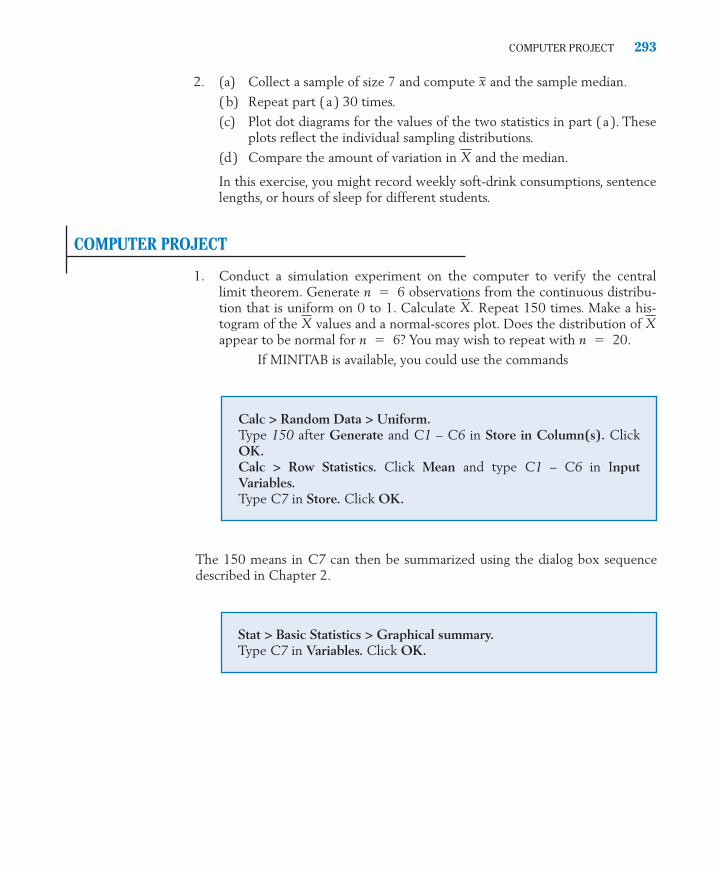
COMPUTER PROJECT 293
Calc > Random Data > Uniform.Type 150 after Generate and C1 – C6 in Store in Column(s). ClickOK.Calc > Row Statistics. Click Mean and type C1 – C6 in Input Variables.Type C7 in Store. Click OK.
Stat > Basic Statistics > Graphical summary.Type C7 in Variables. Click OK.
2. (a) Collect a sample of size 7 and compute and the sample median.
( b) Repeat part ( a ) 30 times.
(c) Plot dot diagrams for the values of the two statistics in part ( a ). Theseplots reflect the individual sampling distributions.
(d) Compare the amount of variation in and the median.
In this exercise, you might record weekly soft-drink consumptions, sentencelengths, or hours of sleep for different students.
COMPUTER PROJECT
1. Conduct a simulation experiment on the computer to verify the centrallimit theorem. Generate n � 6 observations from the continuous distribu-tion that is uniform on 0 to 1. Calculate Repeat 150 times. Make a his-togram of the values and a normal-scores plot. Does the distribution of appear to be normal for n � 6? You may wish to repeat with n � 20.
If MINITAB is available, you could use the commands
XXX.
X
x
The 150 means in C7 can then be summarized using the dialog box sequencedescribed in Chapter 2.
c07.qxd 10/15/09 11:08 AM Page 293

c07.qxd 10/15/09 11:08 AM Page 294

1. Introduction2. Point Estimation of a Population Mean3. Confidence Interval for a Population Mean4. Testing Hypotheses about a Population Mean5. Inferences about a Population Proportion6. Review Exercises
8
Drawing Inferences from Large Samples
c08.qxd 10/15/09 11:09 AM Page 295

Building Strong Evidence from Diverse Individual Cases
One of the major contributions of statistics to modern thinking is the under-standing that information on single, highly variable observations can be com-bined in great numbers to obtain very precise information about a population.
Although each individual is satisfied or not satisfied with his or her job, asample survey can obtain accurate information about the population proportionthat are satisfied.
About 50% are satisfied with their present job.
© Ron Chapple/FPG International/Getty Images.
c08.qxd 10/15/09 11:09 AM Page 296

1. INTRODUCTION
Inferences are generalizations about a population that are made on the basis of asample collected from the population. For instance, a researcher interested inthe growth of pine trees plants 40 seedlings. The heights of these 40 plantswould be a sample that is hopefully representative of the population consistingof all current and future seedlings that could be planted.
More specifically, we begin by modeling the population by a probability dis-tribution which has a numerical feature of interest called a parameter. A ran-dom sample from the population distribution will provide information aboutthe parameter.
The problem of statistical inference arises when we wish to make generaliza-tions about a population when only a sample will be available. Once a sample isobserved, its main features can be determined by the methods of descriptive sum-mary discussed in Chapters 2 and 3. However, more often than not, our principalconcern is with not just the particular data set, but what can be said about thepopulation based on the information extracted from analyzing the sample data. Wecall these generalizations statistical inferences or just inferences.
Consider a study on the effectiveness of a diet program in which 30 partici-pants report their weight loss. We have on hand a sample of 30 measurementsof weight loss. But is the goal of the study confined to this particular group of30 persons? No, it is not. We need to evaluate the effectiveness of the diet pro-gram for the population of potential users. The sample measurements must, ofcourse, provide the basis for any conclusions.
Any inference about a population parameter will involve some uncertainty be-cause it is based on a sample rather than the entire population. To be meaningful, astatistical inference must include a specification of the uncertainty that is deter-mined using the ideas of probability and the sampling distribution of the statistic.
The purpose of an investigation, spelled out in a clear statement of purposeas described in Chapter 1, can reveal the nature of the inference required to an-swer important questions.
The two most important types of inferences are (1) estimation ofparameter(s) and (2) testing of statistical hypotheses. The true value of a pa-rameter is an unknown constant that can be correctly ascertained only by an ex-haustive study of the population, if indeed that were possible. Our objectivemay be to obtain a guess or an estimate of the unknown true value along with adetermination of its accuracy. This type of inference is called estimation of para-meters. An alternative objective may be to examine whether the sample datasupport or contradict the investigator’s conjecture about the true value of theparameter. This latter type of inference is called testing of statistical hypotheses.
1. INTRODUCTION 297
Statistical inference deals with drawing conclusions about population parameters from an analysis of the sample data.
c08.qxd 10/15/09 11:09 AM Page 297

Example 1 Types of Inference: Point Estimation, Interval Estimation, and Testing HypothesesWhat is the degree of participation in community service? A student at alarge midwestern university questioned n = 40 students in her dorm con-cerning the amount of time they spent doing community service during thepast month. The data on times, in hours, are presented in Table 1.
Employing the ideas of Chapter 2, we can calculate a descriptive sum-mary for this set of measurements.
Sample mean Sample standard deviation s � 5.17Sample median First quartile � 1.50 Third quartile � 5.00
However the target of our investigation is not just the particular set of mea-surements recorded, but also concerns the vast population of hours of com-munity service for all students at this university or even similar universities.The population distribution of time is unknown to us. Consequently, parame-ters such as the population mean m and population standard deviation � arealso unknown. If we take the view that the 40 observations represent a ran-dom sample from the population distribution of times, one goal of this studymay be to “learn about m.” More specifically, depending on the purpose of thestudy, we may wish to do one, two, or all three of the following:
1. Estimate a single value for the unknown m (point estimation).
2. Determine an interval of plausible values for m (interval estimation).
3. Decide whether or not the mean time m is 2.6 hours, which wasfound to be the mean time in an earlier study (testing statisticalhypotheses)
Example 2 Inferences about an Unknown ProportionA market researcher wishes to determine what proportion of new-car buyers inher city are satisfied with their new car one year after the purchase. She feels,correctly, that this assessment could be made quickly and effectively by samplinga small fraction of the new-car buyers. The persons selected will be asked if theyare satisfied as opposed to not satisfied. Suppose that a sample of 200 randomlyselected new-car purchasers are interviewed and 168 say they are satisfied.
� 4.00x � 4.55
298 CHAPTER 8/DRAWING INFERENCES FROM LARGE SAMPLES
TABLE 1 Community Service (hours) in Month
0 0 0 0 0 0 0 1 1 12 2 2 2 2 3 3 3 3 44 4 4 5 5 5 5 5 5 55 5 6 6 6 8 10 15 20 25
c08.qxd 10/15/09 11:09 AM Page 298

A descriptive summary of this finding is provided by
Here the target of our investigation is the proportion of new-car purchaserswho are satisfied, p, in the entire collection of new-car buyers in the city. Thevalue of p is unknown. The sample proportion sheds some light on p,but it is subject to some error since it draws only on a part of the population.The investigator would like to evaluate its margin of error and provide an in-terval of plausible values of p.
Also, she may wish to test the hypothesis that proportion satisfied, p, for hercity is not lower than the value given by a nationwide vehicle satisfaction study.
2. POINT ESTIMATION OF A POPULATION MEAN
The object of point estimation is to calculate, from the sample data, a singlenumber that is likely to be close to the unknown value of the parameter. Theavailable information is assumed to be in the form of a random sample , ,. . . , of size n taken from the population. We wish to formulate a statisticsuch that its value computed from the sample data would reflect the value ofthe population parameter as closely as possible.
When we estimate a population mean from a random sample, perhaps themost intuitive estimator is the sample mean,
For instance, to estimate the mean hours of community service in Example 1,we would naturally compute the mean of the sample measurements. Employingthe estimator with the data of Table 1, we get the result hours,which we call a point estimate, or simply an estimate of �.
Without an assessment of accuracy, a single number quoted as an estimatemay not serve a very useful purpose. We must indicate the extent of variabilityin the distribution of the estimator. The standard deviation, alternatively calledthe standard error of the estimator, provides information about its variability.
In order to study the properties of the sample mean as an estimator ofthe population mean m, let us review the results from Chapter 7.
1. E ( X ) � � .
X
x � 4.55X ,
X �X1 � X2 � ��� � X n
n
Xn
X2X1
� .84
Sample proportion satisfied �168200
� .84
2. POINT ESTIMATION OF A POPULATION MEAN 299
A statistic intended for estimating a parameter is called a point estimator,or simply an estimator.The standard deviation of an estimator is called its standard error: S.E.
c08.qxd 10/15/09 11:09 AM Page 299

2.
3. With large n, is nearly normally distributed with mean m and stan-dard deviation
The first two results show that the distribution of is centered around m andits standard error is where s is the population standard deviation and nthe sample size.
To understand how closely is expected to estimate m, we now examinethe third result, which is depicted in Figure 1. Recall that, in a normal distribu-tion, the interval running two standard deviations on either side of the meancontains probability .954. Thus, prior to sampling, the probability is .954 thatthe estimator will be at most a distance from the true parametervalue m. This probability statement can be rephrased by saying that when we are estimating � by the 95.4% error margin is
Use of the probability .954, which corresponds to the multiplier 2 of thestandard error, is by no means universal. The following notation will facilitateour writing of an expression for the 100(1 � a)% error margin, where 1 � a
denotes the desired high probability such as .95 or .90.
A few values of obtained from the normal table appear in Table 2 foreasy reference. To illustrate the notation, suppose we want to determine the90% error margin. We then set 1 � a � .90 so a/2 � .05 and, from Table 2,we have � 1.645. Therefore, when estimating m by the 90% error
margin is 1.645� / √n.
X ,z .05
z a / 2
2� / √ n .X ,
2� / √ nX
X
� / √ n ,X
� / √ n .X
sd( X ) ��
√n so S.E.( X ) �
�
√n.
300 CHAPTER 8/DRAWING INFERENCES FROM LARGE SAMPLES
nσ
µ
2 / nσ2 /
x
Area = .954
Figure 1 Approximate normal distribution of X.
Notation
� Upper a/2 point of standard normal distribution
That is, the area to the right of is a/2, and the area between �and is 1 � a (see Figure 2).z a / 2
z a / 2z a / 2
z a / 2
c08.qxd 10/15/09 11:09 AM Page 300

A minor difficulty remains in computing the standard error of The ex-pression involves the unknown population standard deviation s, but we can es-timate s by the sample standard deviation.
When n is large, the effect of estimating the standard error by canbe neglected. We now summarize.
Example 3 Point Estimation of the Mean Time of Community ServiceFrom the data of Example 1, consisting of 40 measurements of the time de-voted to community service the past month, give a point estimate of thepopulation mean amount of time and state a 95% error margin.
S / √n� / √n
S � � �n
i � 1 (Xi � X )2
n � 1
X.
2. POINT ESTIMATION OF A POPULATION MEAN 301
Figure 2 The notation .z a / 2
1 –
N (0, 1)
0–z
α /2α/2α
/2α z /2α
TABLE 2 Values of
1 � a .80 .85 .90 .95 .99
1.28 1.44 1.645 1.96 2.58z a / 2
z a / 2
Point Estimation of the Mean
Parameter: Population mean m.Data: , . . . , (a random sample of size n)
Estimator: (sample mean)
For large n, the 100(1 � a)% error margin is (If s is unknown, use S in place of s.)
z�/2 � / √n.
S.E.( X ) ��
√n Estimated S.E.( X ) �
S
√n
X
XnX1
c08.qxd 10/15/09 11:09 AM Page 301

SOLUTION The sample mean and the standard deviation computed from the 40 mea-surements in Table 1 are
To calculate the 95% error margin, we set 1 � a � .95 so that a /2 �.025 and � 1.96. Therefore, the 95% error margin is
Our estimate of the population mean time is 4.55 hours per month. Wedo not expect the population mean to be exactly this value and we attach a95% error margin of plus and minus 1.60 hours.
Caution: (a) Standard error should not be interpreted as the “typical” error ina problem of estimation as the word “standard” may suggest. For instance, when S.E. we should not think that the error is likely to be .3,but rather, prior to observing the data, the probability is approximately .954that the error will be within � 2( S.E.) � � .6.
(b) An estimate and its variability are often reported in either of the forms:estimate � S.E. or estimate � 2( S.E.). In reporting a numerical result such as53.4 � 4.6, we must specify whether 4.6 represents S.E., 2 (S.E.), or someother multiple of the standard error.
DETERMINING THE SAMPLE SIZE
During the planning stage of an investigation, it is important to address thequestion of sample size. Because sampling is costly and time-consuming, the in-vestigator needs to know beforehand the sample size required to give the de-sired precision.
In order to determine how large a sample is needed for estimating a popula-tion mean, we must specify
d � Desired error marginand
1 � a � Probability associated with error margin
Referring to the expression for a 100(1 � a)% error margin, we then equate:
z � / 2 �
√n� d
( X � � )( X ) � .3,
1.96 s
√n�
1.96 5.17
√40� 1.60 hours
z a / 2
s � � � ( xi � x )2
39� √ 26.715 � 5.17
x �
� xi
40� 4.55
302 CHAPTER 8/DRAWING INFERENCES FROM LARGE SAMPLES
c08.qxd 10/15/09 11:09 AM Page 302

This gives an equation in which n is unknown. Solving for n, we obtain
which determines the required sample size. Of course, the solution is roundedto the next higher integer, because a sample size cannot be fractional.
This determination of sample size is valid provided n 30, so that thenormal approximation to is satisfactory.
If s is completely unknown, a small-scale preliminary sampling is necessaryto obtain an estimate of s to be used in the formula to compute n.
Example 4 Determining a Sample Size for Collecting Water SamplesA limnologist wishes to estimate the mean phosphate content per unit vol-ume of lake water. It is known from studies in previous years that the stan-dard deviation has a fairly stable value of s � 4. How many water samplesmust the limnologist analyze to be 90% certain that the error of estimationdoes not exceed 0.8 milligrams?
SOLUTION Here s � 4 and 1 � a � .90, so a/2 � .05. The upper .05 point of the N(0, 1) distribution is � 1.645. The tolerable error is d � .8. Computing
we round up to determine that the required sample size is n � 68.
Exercises
n � � 1.645 4.8 �
2
� 67.65
z .05
X
n � � za/2 �
d �2
2. POINT ESTIMATION OF A POPULATION MEAN 303
To be 100(1 � a)% sure that the error of estimation does notexceed d, the required sample size is
n � �z� / 2 �
d �2
| X � � |
8.1 A researcher wants to estimate m , the meannumber of minutes before a person scores over200 on a new computer game. She wishes toget estimates, separately, for each of the groups(a) novices, (b) occasional game players, and(c) expert game players. When using to esti-mate m find the (i) standard error and the (ii)
% error margin for each group.
(a) Novice n � 125 s � 65 98% error margin 4(b) Occasonal n � 47 s � 38 95% error margin 8
100 ( 1 � � )
X
(c) Expert n � 6 s � 20 90% error margin 10
8.2 The same owners operate two coffee shops in alarge building. One is (a) small and the other (b)large. On any day, the number of customers isonly observed for one shop. Determine the pointestimate of m , the mean number of persons servedduring a weekday morning, and the 100(1� a )%error margin, separately, for each shop when
(a) Small n � 65s � 15 1 � a � .95
x � 103
c08.qxd 10/15/09 11:09 AM Page 303

(b) Large n � 45s � 40 1 � a � .975
8.3 Consider the problem of estimating � , themean time per day surfing the Internet, foreach of (a) business, (b) physical, and (c) socialscience majors. Obtain a point estimate of �and the estimated standard error separately foreach of three majors when
(a) Business n � 30
(b) Phy. Sci. n � 25
(c) Social Sci. n � 45
8.4 To study the growth of pine trees at an early stage,a nursery worker records 40 measurements of theheights (cm) of one-year-old red pine seedlings.
The summary Statistics are
n = 40 s = .475 centimeter
Find the (a) point estimate of the population meanheight m , ( b) standard error, and (c) 98% error margin.
8.5 A credit company randomly selected 50 con-tested items and recorded the dollar amountbeing contested. These contested items hadsample mean dollars and s �24.63 dollars. Construct a point estimate forthe population mean contested amount, m , andgive its 90% error margin.
8.6 A manager at a power company monitored theemployee time required to process high-efficiency lamp bulb rebates. A random sampleof 40 applications gave a sample mean time of3.8 minutes and a standard deviation of 1.2 min-utes. Construct a point estimate for the popula-tion mean time to process, m , and give its 90%error margin.
8.7 When estimating m from a large sample, supposethat one has found the 95% error margin of tobe 4.2. From this information, determine:
(a) The estimated S.E. of .
(b) The 90% error margin.
8.8 A small business owner wants to estimate thevalue of her inventory and she needs to estimate,
X
X
x � 95.74
x � 1.715
� ( xi�x )2=194� xi
= 297� ( xi�x )2=103� xi
= 145� ( xi�x )2=116� xi
= 185
x � 260
304 CHAPTER 8/DRAWING INFERENCES FROM LARGE SAMPLES
separately, the mean value of (a) expensiveitems and ( b) other items. She needs the mostaccuracy for expensive items. Determine thesample size n that is required for estimatingthe population mean of each class of items.The population standard deviation s and thedesired error margin are specified.
(a) Expensive 98% error margin 2
(b) Other 90% error margin 5
8.9 When estimating the mean of a population,how large a sample is required in order thatthe 95% error margin be:
(a) of the population standard deviation?
( b) 15% of the population standard deviation?
8.10 Assume that the standard deviation of thenumber of violent incidents in one hour ofchildren’s shows on television is 3.2. An inves-tigator would like to be 99% sure that the truemean number of violent incidents per hour isestimated within 1.4 incidents. For how manyrandomly selected hours does she need tocount the number of violent incidents?
8.11 Referring to Exercise 8.5, suppose that the sur-vey of 50 contested items was, in fact, a pilotstudy intended to give an idea of the popula-tion standard deviation. Assuming s � $25,determine the sample size that is needed forestimating the population mean amount con-tested with a 98% error margin of $5.00.
8.12 Assume that the standard deviation of theheights of five-year-old boys is 3.5 inches. Howmany five-year-old boys need to be sampled ifwe want to be 90% sure that the populationmean height is estimated within .5 inch?
8.13 Let the abbreviation PSLT stand for the per-cent of the gross family income that goes intopaying state and local taxes. Suppose one wantsto estimate the mean PSLT for the populationof all families in New York City with gross in-comes in the range $50,000 to $60,000. If s �2.5, how many such families should be sur-veyed if one wants to be 90% sure of being ableto estimate the true mean PSLT within .5?
8.14 To estimate m with a 90% error margin of 2.9units, one has determined that the requiredsample size is 108. What then is the requiredsample size if one wants the 95% error marginto be 1.8 units?
18
� = 18
� = 135
2.6 1.9 1.8 1.6 1.4 2.2 1.2 1.61.6 1.5 1.4 1.6 2.3 1.5 1.1 1.62.0 1.5 1.7 1.5 1.6 2.1 2.8 1.01.2 1.2 1.8 1.7 0.8 1.5 2.0 2.21.5 1.6 2.2 2.1 3.7 1.7 1.7 1.2Courtesy of Professor Alan Ek.
c08.qxd 10/15/09 11:09 AM Page 304

3. CONFIDENCE INTERVAL FOR A POPULATION MEAN
For point estimation, a single number lies in the forefront even though a stan-dard error is attached. Instead, it is often more desirable to produce an intervalof values that is likely to contain the true value of the parameter.
Ideally, we would like to be able to collect a sample and then use it to cal-culate an interval that would definitely contain the true value of the parameter.This goal, however, is not achievable because of sample-to-sample variation. In-stead, we insist that before sampling the proposed interval will contain the truevalue with a specified high probability. This probability, called the level of confi-dence, is typically taken as .90, .95, or .99.
To develop this concept, we first confine our attention to the constructionof a confidence interval for a population mean m, assuming that the populationis normal and the standard deviation s is known. This restriction helps to sim-plify the initial presentation of the concept of a confidence interval. Later on,we will treat the more realistic case where s is also unknown.
A probability statement about based on the normal distribution providesthe cornerstone for the development of a confidence interval. From Chapter 7, re-call that when the population is normal, the distribution of is also normal. It hasmean m and standard deviation Here m is unknown, but is a knownnumber because the sample size n is known and we have assumed that s is known.
The normal table shows that the probability is .95 that a normal random vari-able will lie within 1.96 standard deviations from its mean. For we then have
as shown in Figure 3.Now, the relation
and
X � � � 1.96 �
√n is the same as X � 1.96
�
√n� �
� � 1.96 �
√n� X is the same as � � X � 1.96
�
√n
P �� � 1.96 �
√n� X � � � 1.96
�
√n� � .95
X,
� / √n� / √n.X
X
3. CONFIDENCE INTERVAL FOR A POPULATION MEAN 305
n– 1.96σµ µ/ n x+ 1.96
0.95
σµ /
nsd = σ /Mean = µ
Figure 3 Normal distribution of X.
c08.qxd 10/15/09 11:09 AM Page 305

as we can see by transposing from one side of an inequality to theother. Therefore, the event
is equivalent to
In essence, both events state that the difference lies between �1.96 and Thus, the probability statement
can also be expressed as
This second form tells us that, before we sample, the random interval fromto will include the unknown parameter m
with a probability of .95. Because s is assumed to be known, both the upperand lower endpoints can be computed as soon as the sample data are available.Guided by the above reasonings, we say that the interval
or its realization is a 95% confidence in-terval for � when the population is normal and s known.
Example 5 Calculating a Confidence Interval—Normal Population s KnownThe daily carbon monoxide (CO) emission from a large production plant willbe measured on 25 randomly selected weekdays. The production process isalways being modified and the current mean value of daily CO emissions m isunknown. Data collected over several years confirm that, for each year, thedistribution of CO emission is normal with a standard deviation of .8 ton.
Suppose the sample mean is found to be tons. Construct a95% confidence interval for the current daily mean emission m.
SOLUTION The population is normal, and the observed value
is a 95% confidence interval for m. Since m is unknown, we cannot determinewhether or not m lies in this interval.
� 2.7 � 1.96 .8
√25 , 2.7 � 1.96
.8
√25 � � ( 2.39, 3.01 ) tons
x � 2.7.
x � 2.7
x � 1.96 � / √n )( x � 1.96 � / √n ,
� X � 1.96 �
√n , X � 1.96
�
√n �
X � 1.96 � / √nX � 1.96 � / √n
P � X � 1.96 �
√n� � � X � 1.96
�
√n � � .95
P � � � 1.96 �
√n� X � � � 1.96
�
√n � � .95
1.96� / √n.� / √nX � �
� X � 1.96 �
√n� � � X � 1.96
�
√n �
� � � 1.96 �
√n� X � � � 1.96
�
√n �
1.96� / √n
306 CHAPTER 8/DRAWING INFERENCES FROM LARGE SAMPLES
c08.qxd 10/15/09 11:09 AM Page 306

Referring to the confidence interval obtained in Example 5, we must notspeak of the probability of the fixed interval (2.39, 3.01) covering the truemean m. The particular interval (2.39, 3.01) either does or does not cover m,and we will never know which is the case.
We need not always tie our discussion of confidence intervals to the choiceof a 95% level of confidence. An investigator may wish to specify a differenthigh probability. We denote this probability by 1 � a and speak of a 100(1 �a)% confidence interval. The only change is to replace 1.96 with , where
denotes the upper a/2 point of the standard normal distribution (i.e., thearea to the right of is a/2, as shown in Figure 2).
In summary, when the population is normal and s is known, a 100(1 � a)%confidence interval for m is given by
INTERPRETATION OF CONFIDENCE INTERVALS
To better understand the meaning of a confidence statement, we use the com-puter to perform repeated samplings from a normal distribution with m � 100and s � 10. Ten samples of size 7 are selected, and a 95% confidence interval
is computed from each. For the first sample,and the interval is 104.3 � 7.4, or 96.9 to 111.7. This and the other intervals areillustrated in Figure 4, where each vertical line segment represents one confidence
x � 104.3x � 1.96 10 / √7
� X � z�/2 �
√n , X � z�/2
�
√n �
z a / 2
z a / 2
z a / 2
3. CONFIDENCE INTERVAL FOR A POPULATION MEAN 307
Yes110
= 100µ
90
0 1 2 3 4 5Sample number
Yes: Interval contains µNo: Interval does not contain µ
6 7 8 9 10
Yes
Yes
Yes Yes
Yes
No
Yes
Yes Yes
Figure 4 Interpretation of the confidence interval for m.
c08.qxd 10/15/09 11:09 AM Page 307

interval. The midpoint of a line is the observed value of for that particularsample. Also note that all the intervals are of the same length2 1.96 Of the 10 intervals shown, 9 cover the true value ofm. This is not surprising, because the specified probability .95 represents thelong-run relative frequency of these intervals covering the true m � 100.
Because confidence interval statements are the most useful way to communi-cate information obtained from a sample, certain aspects of their formulation meritspecial emphasis. Stated in terms of a 95% confidence interval for m, these are:
1. Before we sample, a confidence interval
is a random interval that attempts to cover the true
value of the parameter m.
2. The probability
interpreted as the long-run relative frequency over many repetitions ofsampling asserts that about 95% of the intervals will cover m.
3. Once is calculated from an observed sample, the interval
which is a realization of the random interval, is presented as a 95% con-fidence interval for m . A numerical interval having been determined, itis no longer sensible to speak about the probability of its covering afixed quantity m .
4. In any application we never know if the 95% confidence interval coversthe unknown mean m . Relying on the long-run relative frequency ofcoverage in property 2, we adopt the terminology confidence once theinterval is calculated.
At this point, one might protest, “I have only one sample and I am not re-ally interested in repeated sampling.” But if the confidence estimation tech-niques presented in this text are mastered and followed each time a problem ofinterval estimation arises, then over a lifetime approximately 95% of the inter-vals will cover the true parameter. Of course, this is contingent on the validityof the assumptions underlying the techniques—independent normal observa-tions here.
LARGE SAMPLE CONFIDENCE INTERVALS FOR �
Having established the basic concepts underlying confidence interval state-ments, we now turn to the more realistic situation for which the populationstandard deviation s is unknown. We require the sample size n to be large in
� x � 1.96 �
√n , x � 1.96
�
√n �
x
P � X � 1.96 �
√n� � � X � 1.96
�
√n � � .95
X � 1.96� / √n )
( X � 1.96� / √n ,
� / √ n � 14.8.
X
308 CHAPTER 8/DRAWING INFERENCES FROM LARGE SAMPLES
c08.qxd 10/15/09 11:09 AM Page 308

order to dispense with the assumption of a normal population. The centrallimit theorem then tells us that is nearly normal whatever the form of thepopulation. Referring to the normal distribution of in Figure 5 and the dis-cussion accompanying Figure 2, we again have the probability statement
(Strictly speaking, this probability is approximately 1 � a for a nonnormal pop-ulation.) Even though the interval
will include m with the probability 1 � a, it does not serve as a confidenceinterval because it involves the unknown quantity s. However, because n islarge, replacing with its estimator does not appreciably affect theprobability statement. Summarizing, we find that the large sample confi-dence interval for m has the form
Estimate � ( z Value)(Estimated standard error )
Example 6 A Confidence Interval for the Mean Time of Community ServiceRefer to the data in Example 1, consisting of 40 measurements of the timespent on community service during the past month. The summary statisticsare
S / √n� / √n
� X � z� / 2 �
√n , X � z� / 2
�
√n �
P � X � z � / 2 �
√n� � � X � z� / 2
�
√n � � 1 � �
XX
3. CONFIDENCE INTERVAL FOR A POPULATION MEAN 309
Figure 5 Normal distribution of X.
1 – α
/2
/2
α
– z n
x
/µµ
σα
/2α
/2+ z n/µ σα
Large Sample Confidence Interval for �
When n is large, a 100(1 � a)% confidence interval for m is given by
where S is the sample standard deviation.
�X � z� / 2 S
√n , X � z� / 2
S
√n �
c08.qxd 10/15/09 11:09 AM Page 309

Compute (a) 90% and ( b) 80% confidence intervals for the mean num-ber of hours per month.
SOLUTION The sample size n � 40 is large, so a normal approximation for the distribu-tion of the sample mean is appropriate. From the sample data, we know that
(a) With 1 � a � .90, we have a/2 � .05, and � 1.645,
The 90% confidence interval for the population mean of number ofhours worked m becomes
or approximately (3.2, 5.9) hours per month. This means that wecan be 90% confident that the mean hours per month m is in the in-terval 3.2 to 5.9 hours. We have this confidence because about 90%of the random samples of 40 students would produce intervals
that contain m.
(b) With 1 � a � .80, we have a/2 � .10, and � 1.28, so
The 80% confidence interval for m becomes
(4.55 � 1.05, 4.55 � 1.05) or (3.5, 5.6) hours per month.
Comparing the two confidence intervals, we note that the 80% con-fidence interval is shorter than the 90% interval. A shorter intervalseems to give a more precise location for m but suffers from a lowerlong-run frequency of being correct.
CONFIDENCE INTERVAL FOR A PARAMETER
The concept of a confidence interval applies to any parameter, not just themean. It requires that a lower limit L and an upper limit U be computed fromthe sample data. Then the random interval from L to U must have the specifiedprobability of covering the true value of the parameter. The large sample 100(1 � a)% confidence interval for m has
L � X � z� / 2 S
√n U � X � z� / 2
S
√n
1.28 s
√n�
1.28 5.17
√40� 1.05
z .10
x � 1.645 s / √n
� x � 1.645 s
√n, x � 1.645
s
√n � � ( 4.55 � 1.34, 4.55 � 1.34 )
1.645 s
√n�
1.645 5.17
√ 40� 1.34
z .05
x � 4.55 hours and s � 5.17 hours
X
n � 40 x � 4.55 s � 5.17
310 CHAPTER 8/DRAWING INFERENCES FROM LARGE SAMPLES
c08.qxd 10/15/09 11:09 AM Page 310

Example 7 A Confidence Interval for the Mean Time to Complete a TestMadison recruits for the fire department need to complete a timed test thatsimulates working conditions. It includes placing a ladder against a building,pulling out a section of fire hose, dragging a weighted object, and crawling ina simulated attic environment. The times, in seconds, for recruits to completethe test for Madison firefighter are
425 389 380 421 438 331 368 417 403 416 385 315427 417 386 386 378 300 321 286 269 225 268 317287 256 334 342 269 226 291 280 221 283 302 308296 266 238 286 317 276 254 278 247 336 296 259270 302 281 228 317 312 327 288 395 240 264 246294 254 222 285 254 264 277 266 228 347 322 232365 356 261 293 354 236 285 303 275 403 268 250279 400 370 399 438 287 363 350 278 278 234 266319 276 291 352 313 262 289 273 317 328 292 279289 312 334 294 297 304 240 303 255 305 252 286297 353 350 276 333 285 317 296 276 247 339 328267 305 291 269 386 264 299 261 284 302 342 304336 291 294 323 320 289 339 292 373 410 257 406374 268
Obtain a 95% confidence interval for the mean time of recruits who com-plete the test.
SOLUTION A computer calculation gives
SAMPLE SIZE 158MEAN 307.77STD DEV 51.852
Since 1 � a � .95, a /2 � .025, and � 1.96, the large sample95% confidence interval for m becomes
� � 307.77 � 1.96 51.852
√158, 307.77 � 1.96
51.852
√158 �
� x � z� / 2 s
√n, x � z� / 2
s
√n �
z .025
3. CONFIDENCE INTERVAL FOR A POPULATION MEAN 311
Definition of a Confidence Interval for a Parameter
An interval (L , U ) is a 100(1 � a)% confidence interval for a parameter if
and the endpoints L and U are computable from the sample.
P [ L � Parameter � U ] � 1 � �
c08.qxd 10/15/09 11:09 AM Page 311

or(299.68, 315.86) seconds
When the sample size is large, the sample also contains information onthe shape of the distribution that can be elicited by graphical displays. Figure 6gives the stem-and-leaf display, with the data rounded to two places, accom-panied by the boxplot. The confidence interval pertains to the mean of a pop-ulation with a long right-hand tail.
Exercises
312 CHAPTER 8/DRAWING INFERENCES FROM LARGE SAMPLES
Figure 6 A stem-and-leaf display and boxplot give more information about the form of the population.
approximately how many will cover their respec-tive population means? Explain your reasoning.
8.18 A forester measures 100 needles off a pine treeand finds centimeters and s � 0.7centimeter. She reports that a 95% confidenceinterval for the mean needle length is
or (2.96, 3.24)
(a) Is the statement correct?
(b) Does the interval (2.96, 3.24) cover thetrue mean? Explain.
8.19 In a study on the nutritional qualities of fastfoods, the amount of fat was measured for arandom sample of 35 hamburgers of a particu-lar restaurant chain. The sample mean and stan-dard deviation were found to be 30.2 and 3.8grams, respectively. Use these data to constructa 95% confidence interval for the mean fat con-tent in hamburgers served in these restaurants.
3.1 � 1.96 0.7
√100 to 3.1 � 1.96
0.7
√100
x � 3.1
8.15 Refer to Example 2, Chapter 2, where Table 2records the number of items returned by 30persons to a large discount department store inlate December. The summary statistics are n = 30 s = 1.303.Obtain a 98% confidence interval for m , thepopulation mean number of items returned.
8.16 A company wants to check the consistency ofelectronic copies of signatures for consumer creditpurchases. A sample of 49 electronic signaturesare available from the same customer. One mea-sure of consistency in signing is the total lengththat the script is outside the signature box. Thesample of 49 signatures yielded a mean length of.21 with a standard deviation of .19 centimeter.Obtain a 99% confidence interval for this cus-tomer’s population mean length outside the box.
8.17 Each day of the year, a large sample of cellularphone calls is selected and a 95% confidenceinterval is calculated for the mean length of allcellular phone calls on that day. Of these 365confidence intervals, one for each day of the year,
x � 2.538
* *
STEM-AND-LEAF of TIME N 158LEAF UNIT � 10
2 22222233332 444445555555552 6666666666666666777777777777723
88888888888888889999999999999999
3000000000001111111111
3222222233333333
3444555555
36667777
388888899
4 2223300001111
c08.qxd 10/15/09 11:09 AM Page 312

8.20 In the same study described in Exercise 8.19,the sodium content was also measured for thesampled hamburgers, and the sample mean andstandard deviation were 658 and 47 milligrams,respectively. Determine a 98% confidence inter-val for the true mean sodium content.
8.21 An entomologist sprayed 120 adult Melon flieswith a specific low concentration of malathionand observed their survival times. The mean andstandard deviation were found to be 18.3 and5.2 days, respectively. Use these data to con-struct a 99% confidence interval for the truemean survival time.
8.22 Students are asked about the number of songsthey downloaded from a pay-for-songs Website the last month. From a random sample of39 students, the sample mean was 4.7 with astandard deviation of 3.2.
(a) Obtain a 95% confidence interval for m ,the mean number of songs downloadedby the population of all students.
(b) Does m lie in your interval obtained inPart(a)?
(c) In a long series of repeated experiments,with new samples of 39 students collectedfor each experiment, what proportion ofthe resulting confidence intervals will con-tain the true population mean? Explainyour reasoning.
8.23 The freshness of produce at a super-store is ratedon a scale of 1 to 5 with 5 being very fresh. Froma random sample of 49 customers, the averagescore was 3.8 with a standard deviation of .7.
(a) Obtain a 95% confidence interval for thepopulation mean, m , the mean score forthe distribution of all possible customers.
(b) Does m lie in your interval obtained inPart(a)? Explain.
(c) In a long series of repeated experiments,with new random samples of 49 customerseach day, what proportion of the resultingconfidence intervals will contain the truepopulation mean? Explain your reasoning.
8.24 Referring to Example 7, where the 158 times tocomplete the firefighter test have mean 307.77and standard deviation 51.852, obtain a 99%confidence interval for the mean time of all pos-sible recruits who would complete the test.
3. CONFIDENCE INTERVAL FOR A POPULATION MEAN 313
8.25 Based on a survey of 140 employed persons ina city, the mean and standard deviation of thecommuting distances between home and theprincipal place of business are found to be 8.6and 4.3 miles, respectively. Determine a 90%confidence interval for the mean commutingdistance for the population of all employedpersons in the city.
8.26 A manager at a power company monitored theemployee time required to process high-effi-ciency lamp bulb rebates. A random sample of40 applications gave a sample mean time of3.8 minutes and a standard deviation of 1.2minutes. Construct a 90% confidence intervalfor the mean time to process m.
8.27 A credit company randomly selected 50 con-tested items and recorded the dollar amountbeing contested. These contested items had asample mean dollars and s �24.63 dollars. Construct a 95% confidence in-terval for the mean amount contested, m.
8.28 In a study to determine whether a certain stim-ulant produces hyperactivity, 55 mice were in-jected with 10 micrograms of the stimulant.Afterward, each mouse was given a hyperactiv-ity rating score. The mean score was and s � 2.8. Give a 95% confidence intervalfor the population mean score m.
8.29 Refer to the Statistics in Context section ofChapter 7 concerning monthly changes in theCanadian to U.S. exchange rate. A computer cal-culation gives and s � .0207for the n � 154 monthly changes. Find a 95%confidence interval for the mean monthlychange.
8.30 An employee of an on-campus copy centerwants to determine the mean number ofcopies before a cartridge needs to be replaced.She records the life length in thousands ofcopies for 43 cartridges and obtainsn = 43 s = 1.78 thousand copiesObtain a 90% confidence interval for the pop-ulation mean, � , number of copies in thou-sands before a cartridge should be replaced.
8.31 Refer to the 40 height measurements given inExercise 8.4, which have n = 40 s = .475 centimeter
Calculate a 99% confidence interval for thepopulation mean height.
x � 1.715
x � 8.12
x � �.0017
x � 14.9
x � 95.74
c08.qxd 10/15/09 11:09 AM Page 313

4. TESTING HYPOTHESES ABOUT A POPULATION MEAN
Broadly speaking, the goal of testing statistical hypotheses is to determine if aclaim or conjecture about some feature of the population, a parameter, is stronglysupported by the information obtained from the sample data. Here we illustratethe testing of hypotheses concerning a population mean m. The available data willbe assumed to be a random sample of size n from the population of interest. Fur-ther, the sample size n will be large ( n 30 for a rule of thumb).
The formulation of a hypotheses testing problem and then the steps forsolving it require a number of definitions and concepts. We will introduce thesekey statistical concepts
314 CHAPTER 8/DRAWING INFERENCES FROM LARGE SAMPLES
treated with contaminated sludge. The followingsummary statistics were obtained.
(a) Obtain a 95% confidence interval for thepopulation mean m , amount of PCBs inthe soil.
Answer parts (b), (c), and (d) Yes, No, orCannot tell. Explain your answer.
(b) Does the sample mean PCB content lie inyour interval obtained in part (a)?
(c) Does the population mean PCB contentlie in your interval obtained in part (a)?
(d) It is likely that 95% of the data lie in yourinterval obtained in part (a)?
8.36 A national fast food chain, with thousands offranchise locations, needed to audit the booksat each location. They first selected a sample of50 locations and performed the audit. Theydetermined that a 95% confidence interval forthe mean time to complete an audit is
(28.4 hours, 52.7 hours )
Answer the following questions “Yes,” “No,” or“Cannot tell” and justify your answer.
(a) Does the population mean lie in the in-terval (28.4, 52.7)?
(b) Does the sample mean lie in the interval(28.4, 52.7)?
(c) For a future sample of 50 franchise loca-tions, will the sample mean fall in the in-terval (28.4, 52.7)?
(d) Does 95% of the sample data lie in theinterval (28.4, 52.7)?
x � 3.56 s � .5 ppm
8.32 Radiation measurements on a sample of 65 microwave ovens produced and s � .06. Determine a 95% confidence inter-val for the mean radiation.
8.33 Refer to the data on the growth of femalesalmon in the marine environment in TableD.7 of the Data Bank. A computer calculationgives a 95% confidence interval.
One-Sample Z: Fmarine
Variable N Mean StDev 95.0% CI
Fmarine 40 429.15 41.05 ( 416.43, 441.87)
(a) Does the 95% confidence interval coverthe true mean growth of all femalesalmon in that marine environment?
(b) Why are you 95% confident that the inter-val (416.43, 441.87) covers the true mean?
8.34 Refer to the data on the girth, in centimeters,of grizzly bears in Table D.8 of the Data Bank.A computer calculation gives
One-Sample Z: Girth
Variable N Mean StDev 95.0% CI
Girth 61 93.39 21.79 ( 87.93, 98.86)
(a) Does the 95% confidence interval coverthe true mean girth of all grizzly bears inthe area of the study? Explain.
(b) Why are you 95% confident that the in-terval (87.93, 98.86) covers the truemean?
8.35 The amount of PCBs (polychlorinated biphenyls)was measured in 40 samples of soil that were
x � .11
c08.qxd 10/15/09 11:09 AM Page 314

Null hypothesis and the alternative hypothesis
Type I and Type II errors
Level of significance
Rejection region
P–value
in the context of a specific problem to help integrate them with intuitivereasoning.
PROBLEM: Can an upgrade reduce the mean transaction time at auto-mated teller machines? At peak periods, customers are subject to unreason-ably long waits before receiving cash. To help alleviate this difficulty, thebank wants to reduce the time it takes a customer to complete a transac-tion. From extensive records, it is found that the transaction times have adistribution with mean 270 and standard deviation 24 seconds. The tellermachine vendor suggests that a new software and hardware upgrade will re-duce the mean time for a customer to complete a transaction. For experi-mental verification, a random sample of 38 transaction times will be takenat a machine with the upgrade and the sample mean calculated. Howshould the result be used toward a statistical validation of the claim that thetrue (population) mean transaction time is less than 270 seconds?
Whenever we seek to establish a claim or conjecture on the basis of strongsupport from sample data, the problem is called one of hypothesis testing.
FORMULATING THE HYPOTHESES
In the language of statistics, the claim or the research hypothesis that we wishto establish is called the alternative hypothesis . The opposite statement,one that nullifies the research hypothesis, is called the null hypothesis . Theword “null” in this context means that the assertion we are seeking to establishis actually void.
Our initial question, “Is there strong evidence in support of the claim?” nowtranslates to “Is there strong evidence for rejecting ?” The first version typi-cally appears in the statement of a practical problem, whereas the second ver-sion is ingrained in the conduct of a statistical test. It is crucial to understand thecorrespondence between the two formulations of a question.
Before claiming that a statement is established statistically, adequate evi-dence from data must be produced to support it. A close analogy can be made
H0
H0
H1
X
4. TESTING HYPOTHESES ABOUT A POPULATION MEAN 315
Formulation of and
When our goal is to establish an assertion with substantive support ob-tained from the sample, the negation of the assertion is taken to be thenull hypothesis and the assertion itself is taken to be the alternativehypothesis .H1
H0
H1H0
c08.qxd 10/15/09 11:09 AM Page 315

to a criminal court trial where the jury clings to the null hypothesis of “notguilty” unless there is convincing evidence of guilt. The intent of the hearings isto establish the assertion that the accused is guilty, rather than to prove that heor she is innocent.
Once and are formulated, our goal is to analyze the sample data inorder to choose between them.
A decision rule, or a test of the null hypothesis, specifies a course of actionby stating what sample information is to be used and how it is to be used inmaking a decision. Bear in mind that we are to make one of the following twodecisions:
Rejection of amounts to saying that is substantiated, whereas nonre-jection or retention of means that fails to be substantiated. A key point isH1H0
H1H0
H1H0
316 CHAPTER 8/DRAWING INFERENCES FROM LARGE SAMPLES
Testing StatisticalCourt Trial Hypothesis
Requires strong Conjecture (research evidence to establish: Guilt. hypothesis).
Null hypothesis ( ): Not guilty. Conjecture is false.
Alternative hypothesis( ): Guilty. Conjecture is true.
Attitude: Uphold “not guilty” Retain the nullunless there is a strong hypothesis unless itevidence of guilt. makes the sample data
very unlikely to happen.
False rejection of is a more serious error than failing to reject whenis true.H1
H0H0
H1
H0
Decisions
EitherReject and conclude that is substantiated
orRetain and conclude that fails to be substantiatedH1H0
H1H0
c08.qxd 10/15/09 11:09 AM Page 316

that a decision to reject must be based on strong evidence. Otherwise, theclaim could not be established beyond a reasonable doubt.
In our problem of evaluating the upgraded teller machine, let m be the pop-ulation mean transaction time. Because m is claimed to be lower than 270 sec-onds, we formulate the alternative hypothesis as :m � 270. According tothe description of the problem, the researcher does not care to distinguish be-tween the situations that m � 270 and m 270 for the claim is false in eithercase. For this reason, it is customary to write the null hypothesis simply as astatement of no difference. Accordingly, we formulate the
Testing Problem
TEST CRITERION AND REJECTION REGION
Naturally, the sample mean calculated from the measurements of n � 38 ran-domly selected transaction times, ought to be the basis for rejecting or not. Thequestion now is: For what sort of values of should we reject ? Because theclaim states that m is low (a left-sided alternative), only low values of can contra-dict in favor of . Therefore, a reasonable decision rule should be of the form
This decision rule is conveniently expressed as where R stands forthe rejection of . Also, in this context, the set of outcomes is called therejection region or critical region, and the cutoff point c is called the critical value.
The cutoff point c must be specified in order to fully describe a decisionrule. To this end, we consider the case when holds, that is, m � 270. Rejec-tion of would then be a wrong decision, amounting to a false acceptance ofthe claim—a serious error. For an adequate protection against this kind of error,we must ensure that is very small when m � 270. For example,suppose that we wish to hold a low probability of a � .05 for a wrong rejec-tion of . Then our task is to find the c that makes
We know that, for large n, the distribution of is approximately normalwith mean m and standard deviation whatever the form of the underly-ing population. Here n � 38 is large, and we initially assume that s is known.Specifically, we assume that s � 24 seconds, the same standard deviation aswith the original money machines. Then, when m � 270, the distribution of is N so
has the N(0, 1) distribution.
Z �X � 270
24 / √38
( 270, 24 / √38 )X
� / √n ,X
P [ X � c ] � .05 when � � 270
H0
P [ X � c ]
H0
H0
[ X � c ]H0
R : X � c ,
Retain H0 if X cReject H0 if X � c
H1H0
XH0X
H0
X ,
Test H0 : � � 270 versus H1
: � � 270
H1
H1
H0
4. TESTING HYPOTHESES ABOUT A POPULATION MEAN 317
c08.qxd 10/15/09 11:09 AM Page 317

Because the cutoff c on the scale must be1.645 standard deviations below � 270 or
Our decision rule is now completely specified by the rejection region (seeFigure 7)
that has a � .05 as the probability of wrongly rejecting .Instead of locating the rejection region on the scale of we can cast the
decision criterion on the standardized scale as well:
and set the rejection region as (see Figure 7). This form ismore convenient because the cutoff �1.645 is directly read off the normaltable, whereas the determination of c involves additional numerical work.
A test is completely specified by a test statistic and the rejection region.
R : Z � �1.645
Z �X � � 0
� / √n�
X � 270
24 / √38
X ,H0
R : X � 263.6
c � 270 � 1.645 � 24
√38� � 270 � 6.40 � 263.60
m 0
xP [ Z � �1.645] � .05,
318 CHAPTER 8/DRAWING INFERENCES FROM LARGE SAMPLES
.05
R: X ≤ 263.6
R: Z ≤ –1.645 0 z
270.0 x
Figure 7 Rejection region with the cutoff c � 263.6.
The random variable whose value serves to determine the action iscalled the test statistic.
A test of the null hypothesis is a course of action specifying the set of values of a test statistic for which is to be rejected.
This set is called the rejection region of the test.H0X ,
X
c08.qxd 10/15/09 11:09 AM Page 318

TWO TYPES OF ERROR AND THEIR PROBABILITIES
Up to this point we only considered the probability of rejecting when, infact, is true and illustrated how a decision rule is determined by setting thisprobability equal to .05. The following table shows all the consequences thatmight arise from the use of a decision rule.
In particular, when our sample-based decision is to reject , either wehave a correct decision (if is true) or we commit a Type I error (if istrue). On the other hand, a decision to retain either constitutes a correct de-cision (if is true) or leads to a Type II error. To summarize:
In our problem of evaluating the upgraded teller machine, the rejection re-gion is of the form so that,
� P [ X c ] when � � 270 ( H1 true )
� � P [ X � c ] when � � 270 ( H0 true )
R : X � c ;
H0
H0
H0H1
H0
H0
H0
4. TESTING HYPOTHESES ABOUT A POPULATION MEAN 319
Unknown True Situation
Decision Based True Trueon Sample m � 270 m � 270
Reject Wrong rejection of Correct decision(Type I error)
Retain Correct decision Wrong retention of (Type II error)
H0H0
H0H0
H1H0
Two Types of Error
Type I error: Rejection of when is true
Type II error: Nonrejection of when is true
a � Probability of making a Type I error(also called the level of significance)
b � Probability of making a Type II error
H1H0
H0H0
c08.qxd 10/15/09 11:09 AM Page 319

Of course, the probability b depends on the numerical value of m that pre-vails under . Figure 8 shows the Type I error probability a as the shaded areaunder the normal curve that has m � 270 and the Type II error probability b asthe shaded area under the normal curve that has m � 262, a case of beingtrue.
From Figure 8, it is apparent that no choice of the cutoff c can minimizeboth the error probabilities a and b. If c is moved to the left, a gets smaller but bgets larger, and if c is moved to the right, just the opposite effects take place. Inview of this dilemma and the fact that a wrong rejection of is the more seri-ous error, we hold a at a predetermined low level such as .10, .05, or .01 whenchoosing a rejection region. We will not pursue the evaluation of b, but we donote that if the b turns out to be uncomfortably large, the sample size must beincreased.
PERFORMING A TEST
When determining the rejection region for this example, we assumed that s �24 seconds, the same standard deviation as with the original money machines.Then, when m � 270, the distribution of is and the rejectionregion was arrived at by fixing a � .05 and referring
to the standard normal distribution.In practice, we are usually not sure about the assumption that s � 24, the
standard deviation of the transaction times using the upgraded machine, is thesame as with the original teller machine. But that does not cause any problemas long as the sample size is large. When n is large (n 30), the normal ap-proximation for remains valid even if s is estimated by the sample standarddeviation S. Therefore, for testing versus with levelH1 : � � �0H0 : � � �0
X
Z �X � 270
24 / √38
R : X � 263.6N ( 270, 24 / √38 )X
H0
H1
H1
320 CHAPTER 8/DRAWING INFERENCES FROM LARGE SAMPLES
H0 true
H1 true
Retain H0Reject H0
= 270c xµα
β
= 262 c xµ
Figure 8 The error probabilities a and b.
c08.qxd 10/15/09 11:09 AM Page 320

of significance a, we employ the test statistic
and set the rejection region This test is commonly called a largesample normal test or a Z test.
Example 8 A One-Sided Test of Hypotheses to Establish That m � 270Referring to the automated teller machine transaction times, suppose that, fromthe measurements of a random sample of 38 transaction times, the samplemean and standard deviation are found to be 261 and 22 seconds, respectively.Test the null hypothesis versus using a 2.5% levelof significance and state whether or not the claim m � 270 is substantiated.
SOLUTION Because n � 38 and the null hypothesis specifies that m has the value �270, we employ the test statistic
The rejection region should consist of small values of Z because isleft-sided. For a 2.5% level of significance, we take a � .025, and since
� 1.96, the rejection region is (see Figure 9)
With the observed values and s � 22, we calculate the teststatistic
Because this observed z is in R, the null hypothesis is rejected at the levelof significance a � .025. We conclude that the claim of a reduction in themean transaction time is strongly supported by the data.
P–VALUE: HOW STRONG IS A REJECTION OF ?
Our test in Example 8 was based on the fixed level of significance a � .025,and we rejected because the observed z � � 2.52 fell in the rejection re-gion A strong evidence against emerged due to the fact thatH0R : Z � �1.96.
H0
H0
z �261 � 270
22 / √38� �2.52
x � 261
R : Z � �1.96.z .025
H1
Z �X � 270
S / √38
m 0
H1 :� � 270H0 :� � 270
R : Z � �z� .
Z �X � �0
S / √n
4. TESTING HYPOTHESES ABOUT A POPULATION MEAN 321
0–1.96 z
.025
Figure 9 Rejection region for Z.
c08.qxd 10/15/09 11:09 AM Page 321

a small a was used. The natural question at this point is: How small an a couldwe use and still arrive at the conclusion of rejecting ? To answer this ques-tion, we consider the observed z � � 2.52 itself as the cutoff point (criticalvalue) and calculate the rejection probability
The smallest possible a that would permit rejection of , on the basis of theobserved is therefore .0059 (see Figure 10). It is called the signifi-cance probability or P–value of the observed z. This very small P–value, .0059,signifies a strong rejection of or that the result is highly statistically significant.H0
z � �2.52,H0
P [ Z � �2.52] � .0059
H0
322 CHAPTER 8/DRAWING INFERENCES FROM LARGE SAMPLES
The Steps for Testing Hypotheses
1. Formulate the null hypothesis and the alternative hypothesis .
2. Test criterion: State the test statistic and the form of the rejection region.
3. With a specified a, determine the rejection region.
4. Calculate the test statistic from the data.
5. Draw a conclusion: State whether or not is rejected at the speci-fied a and interpret the conclusion in the context of the problem.Also, it is a good statistical practice to calculate the P–value andstrengthen the conclusion.
H0
H1H0
The P–value is the probability, calculated under , that the test statistictakes a value equal to or more extreme than the value actually observed.
H0
0–1.96 z
.0059
Figure 10 P–value with left-sided rejection region.
The P–value serves as a measure of the strength of evidence against . Asmall P–value means that the null hypothesis is strongly rejected or the result ishighly statistically significant.
Our illustrations of the basic concepts of hypothesis tests thus far focused ona problem where the alternative hypothesis is of the form :m � , called aleft-sided alternative. If the alternative hypothesis in a problem states that the truem is larger than its null hypothesis value of , we formulate the right-sided alter-native :m and use a right-sided rejection region R: Z � .zam 0H1
m 0
m 0H1
H0
c08.qxd 10/15/09 11:09 AM Page 322

We illustrate the right-sided case and the main steps for conducting a statis-tical test as summarized above.
Example 9 Evaluating a Weight Loss Diet—Calculation of a P–ValueA brochure inviting subscriptions for a new diet program states that the partic-ipants are expected to lose over 22 pounds in five weeks. Suppose that, fromthe data of the five-week weight losses of 56 participants, the sample mean andstandard deviation are found to be 23.5 and 10.2 pounds, respectively. Couldthe statement in the brochure be substantiated on the basis of these findings?Test with a � .05. Also calculate the P–value and interpret the result.
SOLUTION Let m denote the population mean weight loss from five weeks of participa-tion in the program. Because our aim is to substantiate the assertion that m 22 pounds, we formulate the hypotheses
�m � 22 versus �m 22
The sample size is n � 56. Denoting the sample mean weight loss ofthe 56 participants by and the standard deviation by S, our test statistic is
Because H1 is right-sided, the rejection region should be of the form R : Z � c. Because the test with level of significance .05 hasthe rejection region (see Figure 11) R : Z � 1.645.
With the observed values and we calculate
Because 1.10 is not in R, we do not reject the null hypothesis. We con-clude that, with level of significance a � .05, the stated claim that m 22is not substantiated.
Because our observed z is 1.10 and larger values are more extreme, thesignificance probability of this result is
P–value � P [ Z � 1.10] = .1357 ( from the normal table )
z �23.5 � 22
10.2 / √56� 1.10
s � 10.2,x � 23.5
z.05 � 1.645,
Z �X � � 0
S / √n�
X � 22
S / √56
X
H1H0
4. TESTING HYPOTHESES ABOUT A POPULATION MEAN 323
.05
0 1.645 z
Figure 11 Right-sided rejection region with a � .05.
c08.qxd 10/15/09 11:09 AM Page 323

That is, .1357 is the smallest a at which could be rejected (Figure 12).This is not ordinarily considered a negligible chance so we conclude that thedata do not provide a strong basis for rejection of .
The preceding hypotheses are called one-sided hypotheses, because the val-ues of the parameter m under the alternative hypothesis lie on one side of thoseunder the null hypothesis. The corresponding tests are called one-sided tests orone-tailed tests. By contrast, we can have a problem of testing the null hypothesis
: m �
versus the two-sided alternative or two-sided hypothesis
: m �
Here is to be rejected if is too far away from in either direction, thatis, if Z is too small or too large. For a level a test, we divide the rejection proba-bility a equally between the two tails and construct the rejection region
R : Z � � or Z �
which can be expressed in the more compact notation
Example 10 Testing Hypotheses about the Mean Time of Community ServiceConsider the data of Example 1 concerning 40 observations on time devotedto community service in the past month. Do these data indicate that the pop-ulation mean time is different from 2.6 hours?
SOLUTION We are seeking evidence in support of m � 2.6 so the hypotheses should beformulated as
: m � 2.6 versus : m � 2.6
The sample size n � 40 being large, we will employ the test statistic
Z �X � � 0
S / √n�
X � 2.6
S / √40
H1H0
R : � Z � � z�/2
z� / 2z� / 2
m 0XH0
m 0H1
m 0H0
H0
H0
324 CHAPTER 8/DRAWING INFERENCES FROM LARGE SAMPLES
0 1.10 1.645 z
.1357
Figure 12 P–value with right-sidedrejection region.
c08.qxd 10/15/09 11:09 AM Page 324

The two-sided form of dictates that the rejection region must also betwo-sided.
Let us choose a � .05, then a /2 � .025 and � 1.96. Conse-quently, for a � .05, the rejection region is ( see Figure 13)
From Example 1, and so the observed value of the teststatistic is
Because is larger than 1.96, we reject at a � .05.In fact, the large value seems to indicate a much stronger re-
jection of than that arising from the choice of a � .05. How small an acan we set and still reject ? This is precisely the idea underlying the signifi-cance probability or the P–value. We calculate (see Figure 14)
P–value
� 2 .0084 � .0168
� P [ Z � �2.39 ] � P [ Z � 2.39 ]
� P [ � Z � � 2.39 ]
H0
H0
� z � � 2.39H0� z � � 2.39
z �x � � 0
s / √n�
4.55 � 2.6
5.17 / √40� 2.39
s � 5.17,x � 4.55
R : � Z � � 1.96
z .025
H1
4. TESTING HYPOTHESES ABOUT A POPULATION MEAN 325
.025
0–1.96 1.96 z
.025
Figure 13 Two-sided rejection regionwith a � .05.
Figure 14 P–value with two-sided rejection region.
.0084 .0084
–1.96 –1.960 z•
c08.qxd 10/15/09 11:09 AM Page 325

With a as small as .0138, is still rejected. This very small P–value givesstrong support for .
In summary:
Because the central limit theorem prevails for large n, no assumption is re-quired as to the shape of the population distribution.
Exercises
H1
H0
326 CHAPTER 8/DRAWING INFERENCES FROM LARGE SAMPLES
Large Sample Tests for �
When the sample size is large, a Z test concerning m is based on the nor-mal test statistic
The rejection region is one- or two-sided depending on the alternative hypothesis. Specifically,
H1 : � � �0 R : � Z � � z�/2
H1 : � � �0 R : Z � �z�
H1 : � �0 requires R : Z � z�
Z �X � � 0
S / √n
8.37 Stated here are some claims or research hy-potheses that are to be substantiated by sam-ple data. In each case, identify the null hypoth-esis and the alternative hypothesis interms of the population mean m.
(a) The mean time a health insurance com-pany takes to pay claims is less than 14working days.
(b) The average person watching a movie at alocal multiplex theater spends over $4.50on refreshments.
(c) The mean hospital bill for a birth in thecity is less than $5000.
(d) The mean time between purchases of abrand of mouthwash by loyal customersis different from 60 days.
H1H0
8.38 From an analysis of the sample data, supposethat the decision has been to reject the null hy-pothesis. In the context of each part (a–d) ofExercise 8.37, answer the following questions:
In what circumstance is it a correct decision?
When is it a wrong decision, and what typeof error is then made?
8.39 From an analysis of the sample data, supposethat the decision has been made to retain thenull hypothesis. In the context of each part(a–d) of Exercise 8.37, answer the followingquestions.
In what circumstance is it a correct decision?
When is it a wrong decision, and what typeof error is then made?
c08.qxd 10/15/09 11:09 AM Page 326

8.40 For each situation (a–d) in Exercise 8.37, statewhich of the following three forms of the re-jection region is appropriate when s is known.
8.41 Each part (a–d) of this problem gives thepopulation standard deviation s, the state-ment of a claim about m, the sample size n ,and the desired level of significance a .Formulate (i) the hypotheses, (ii) the test sta-tistic Z, and (iii) the rejection region. (Theanswers to part (a) are provided.)
(a) s � 2 claim: m 30, n � 55, a � .05[Answers: (i)
(ii) (iii)
(b) s � .085 claim: m � .15 n � 125 a � .025(c) s � 8.6 claim: m � 80 n � 38 a � .01(d) s � 1.23 claim: m � 0 n � 40 a � .06
8.42 Suppose that the observed values of the samplemean in the contexts of parts (a–d) of Exercise8.41 are given as follows. Calculate the test statis-tic Z and state the conclusion with the specified a.
(a) (b)
(c) (d)
8.43 A market researcher wants to perform a testwith the intent of establishing that his com-pany’s medium pump bottle of soap has amean life greater than 40 days. The sample sizeis 70 and he knows that s � 5.6.(a) If you set the rejection region to be
R : what is the level of sig-nificance of your test?
(b) Find the numerical value of c so that the testR : has a 5% level of significance.
8.44 With reference to Exercise 8.15, perform a testwith the intent of establishing that the meannumber of items returned is greater than 2.0.Take � = .02.
8.45 With reference to Exercise 8.44,
(a) test: m � 2.0 : m � 2.0
with a � .02.H1H0
X � c
X � 41.31,
x � �.59x � 77.35
x � .136x � 30.54
R : Z � 1.645 ]Z �X � 30
2 / √55
H0 :� � 30, H1 :� 30
R : � X � � 0 � � c ( two-sided )
R : X � c ( right-sided ) R : X � c ( left-sided )
4. TESTING HYPOTHESES ABOUT A POPULATION MEAN 327
(b) Based on your decision in Part (a), whaterror could you have possibly made?Explain in the context of the problem.
8.46 An investigator at a large midwestern univer-sity wants to determine the typical weeklyamount of time students work on part-timejobs. More particularly, he wants to test thenull hypothesis that the mean time is 15 hoursversus a two-sided alternative. A sample of 39students who hold part-time jobs is summa-rized by the computer output
Descriptive Statistics: hours
Variable N Mean Median StDevHours 39 16.69 15.00 7.61
(a) Perform the hypothesis test at the 1%level of significance.
(b) Calculate the significance probability andinterpret the result.
8.47 Refer to the data on the growth of femalesalmon growth in the marine environment inTable D.7 of the Data Bank. A computer cal-culation for a test of : m � 411 versus
: m � 411 is given below.
Test of mu = 411 vs mu not = 411
Variable N Mean StDevFmarine 40 429.15 41.05
Variable Z PFmarine 2.80 0.005
(a) What is the conclusion if you test with a � .01?
(b) What mistake could you have made inpart (a)?
(c) Before you collected the data, what wasthe probability of making the mistake inpart (a)?
(d) Give a long-run relative frequency inter-pretation of the probability in part (c).
(e) Give the P–value of your test with a � .01.
8.48 Refer to the data on the girth, in centimeters, ofgrizzly bears in Table D.8 of the Data Bank. Acomputer calculation for a test of : m � 100centimeters versus : m � 100 givesH1
H0
H1
H0
c08.qxd 10/15/09 11:09 AM Page 327
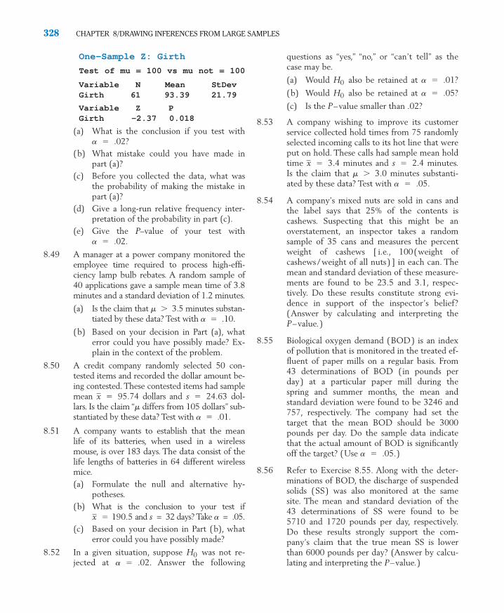
One-Sample Z: Girth
Test of mu = 100 vs mu not = 100
Variable N Mean StDevGirth 61 93.39 21.79
Variable Z PGirth -2.37 0.018
(a) What is the conclusion if you test witha � .02?
(b) What mistake could you have made inpart (a)?
(c) Before you collected the data, what wasthe probability of making the mistake inpart (a)?
(d) Give a long-run relative frequency inter-pretation of the probability in part (c).
(e) Give the P–value of your test with a � .02.
8.49 A manager at a power company monitored theemployee time required to process high-effi-ciency lamp bulb rebates. A random sample of40 applications gave a sample mean time of 3.8minutes and a standard deviation of 1.2 minutes.
(a) Is the claim that m 3.5 minutes substan-tiated by these data? Test with a � .10.
(b) Based on your decision in Part (a), whaterror could you have possibly made? Ex-plain in the context of the problem.
8.50 A credit company randomly selected 50 con-tested items and recorded the dollar amount be-ing contested. These contested items had samplemean dollars and dol-lars. Is the claim “m differs from 105 dollars” sub-stantiated by these data? Test with a � .01.
8.51 A company wants to establish that the meanlife of its batteries, when used in a wirelessmouse, is over 183 days. The data consist of thelife lengths of batteries in 64 different wirelessmice.(a) Formulate the null and alternative hy-
potheses.(b) What is the conclusion to your test if
and s = 32 days? Take a = .05.(c) Based on your decision in Part (b), what
error could you have possibly made?
8.52 In a given situation, suppose was not re-jected at a � .02. Answer the following
H0
x � 190.5
s � 24.63x � 95.74
328 CHAPTER 8/DRAWING INFERENCES FROM LARGE SAMPLES
questions as “yes,” “no,” or “can’t tell” as thecase may be.
(a) Would also be retained at a � .01?
(b) Would also be retained at a � .05?
(c) Is the P–value smaller than .02?
8.53 A company wishing to improve its customerservice collected hold times from 75 randomlyselected incoming calls to its hot line that wereput on hold. These calls had sample mean holdtime minutes and minutes.Is the claim that m 3.0 minutes substanti-ated by these data? Test with a � .05.
8.54 A company’s mixed nuts are sold in cans andthe label says that 25% of the contents iscashews. Suspecting that this might be anoverstatement, an inspector takes a randomsample of 35 cans and measures the percentweight of cashews [ i.e., 100(weight ofcashews / weight of all nuts) ] in each can. Themean and standard deviation of these measure-ments are found to be 23.5 and 3.1, respec-tively. Do these results constitute strong evi-dence in support of the inspector’s belief?(Answer by calculating and interpreting theP–value.)
8.55 Biological oxygen demand (BOD) is an indexof pollution that is monitored in the treated ef-fluent of paper mills on a regular basis. From43 determinations of BOD (in pounds perday) at a particular paper mill during thespring and summer months, the mean andstandard deviation were found to be 3246 and757, respectively. The company had set thetarget that the mean BOD should be 3000pounds per day. Do the sample data indicatethat the actual amount of BOD is significantlyoff the target? (Use a � .05.)
8.56 Refer to Exercise 8.55. Along with the deter-minations of BOD, the discharge of suspendedsolids (SS) was also monitored at the samesite. The mean and standard deviation of the43 determinations of SS were found to be5710 and 1720 pounds per day, respectively.Do these results strongly support the com-pany’s claim that the true mean SS is lowerthan 6000 pounds per day? (Answer by calcu-lating and interpreting the P–value.)
s � 2.4x � 3.4
H0
H0
c08.qxd 10/15/09 11:09 AM Page 328

5. INFERENCES ABOUT A POPULATION PROPORTION
The reasoning leading to estimation of a mean also applies to the problem of es-timation of a population proportion. Example 2 considers sampling n � 200new car buyers to infer about the proportion of the population that is satisfiedafter one year. When n elements are randomly sampled from the population, thedata will consist of the count X of the number of sampled elements possessingthe characteristic. Common sense suggests the sample proportion
as an estimator of p. The hat notation reminds us that is a statistic.When the sample size n is only a small fraction of the population size, the
sample count X has the binomial distribution with mean np and standard devia-tion where Recall from Chapter 6 that, when n is large, thebinomial variable X is well approximated by a normal with mean np and standard deviation That is,
is approximately standard normal. This statement can be converted into a state-ment about proportions by dividing the numerator and the denominator by n.In particular,
This last form, illustrated in Figure 15, is crucial to all inferences about a popu-lation proportion p. It shows that is approximately normally distributed with mean p and standard deviation √p q / n.
p
Z �(X � n p ) / n
(√ n p q ) / n�
p � p
√ p q / n
Z �X � n p
√ n p q
√ n p q .
q � 1 � p .√ n p q ,
p
p �Xn
5. INFERENCES ABOUT A POPULATION PROPORTION 329
1 – α
/2
/2
α
p – z pq/nα
/2α
/2p + z
p p
pq/nα
ˆ
Figure 15 Approximate normal distribution of .p
c08.qxd 10/15/09 11:09 AM Page 329

POINT ESTIMATION OF p
Intuitively, the sample proportion is a reasonable estimator of the populationproportion p. When the count X has a binomial distribution,
Since the properties of expectation give
In other words, the sampling distribution of has a mean equal to the popula-tion proportion. The second result shows that the standard error of the estima-tor is
The estimated standard error can be obtained by substituting the sample esti-mate for p and for q in the formula, or
When n is large, prior to sampling, the probability is approximately .954 thatthe error of estimation will be less than 2 (estimated S.E.).
Example 11 Estimating the Proportion of PurchasersA large mail-order club that offers monthly specials wishes to try out anew item. A trial mailing is sent to a random sample of 250 members se-lected from the list of over 9000 subscribers. Based on this sample mailing,70 of the members decide to purchase the item. Give a point estimate of
� p � p �
Estimated S.E.( p ) � � p qn
q � 1 � pp
S.E.( p) � � pqn
p
p
sd( p) � √pq / n E( p) � p
p � X / n ,
E ( X ) � n p sd ( X ) � √ n p q
p
330 CHAPTER 8/DRAWING INFERENCES FROM LARGE SAMPLES
Point Estimation of a Population Proportion
Parameter: Population proportion p
Data: X � Number having the characteristic in a random sample of size n
For large n, an approximate 100(1 � a)% error margin is z � / 2 √ p q /n .
S.E.( p ) � � p qn
and estimated S.E. ( p ) � � p qn
Estimator: p �Xn
c08.qxd 10/15/09 11:09 AM Page 330

the proportion of club members that could be expected to purchase theitem and attach a 95.4% error margin.
SOLUTION The number in the sample represents only a small fraction of the total mem-bership, so the count can be treated as if it were a binomial variable.
Here n � 250 and X � 70, so the estimate of the population proportion is
Therefore, the estimated proportion is with a 95.4% error marginof .06 (rounded to two decimals).
p � .28,
95.4% error margin � 2 .028 � .056
Estimated S.E.( p ) � � p qn
� � .28 .72250
� .028
p �70
250� .28
5. INFERENCES ABOUT A POPULATION PROPORTION 331
CONFIDENCE INTERVAL FOR p
A large sample confidence interval for a population proportion can be obtainedfrom the approximate normality of the sample proportion . Since is nearlynormal with mean p and standard deviation the random interval √ p q / n ,
pp
Novel Collection of Count Data
Producers of breakfast cereals continually experiment with new products.Each promising new cereal must be market-tested on a sample of poten-tial purchasers. An added twist here is that youngsters are a major compo-nent of the market. In order to elicit accurate information from youngpeople, one firm developed a smiling face scale.
After tasting a new product, respondents are asked to check one boxto rate the taste. A good product should have most of the youngsters responding in the top two boxes. Grouping these into a single highest category and the lower three boxes into a lower category, we are in thesituation of estimating the proportion of the market population thatwould rate taste in the highest category.
Out of a sample of 42 youngsters, 30 rated a new cereal in the topcategory.
c08.qxd 10/15/09 11:09 AM Page 331

is a candidate. However, the standard deviation involves the
unknown parameter p, so we use the estimated standard deviation toset the endpoints of the confidence interval. Notice again that the commonform of the confidence interval is
Example 12 A Confidence Interval for the Proportion SatisfiedConsider the data in Example 2 where 168 out of a random sample of 200new car purchasers were satisfied with their car after one year. Compute a95% confidence interval for the population proportion of satisfied new carpurchasers.
SOLUTION The sample size n � 200 is large so a normal approximation to the distribu-tion of is justified. Since 1 � a � .95, we have a /2 � .025 and �1.96. The observed and Wecalculate
Therefore, a 95% confidence interval for the population proportion of satis-fied new-car buyers is .840 � .051, or ( .789, .891).
Because our procedure will produce true statements 95% of the time, wecan be 95% confident that the proportion of satisfied new-car buyers is be-tween .789 and .891.
DETERMINING THE SAMPLE SIZE
Note that, prior to sampling, the numerical estimate of p is not avail-able. Therefore, for a 100(1 � a)% error margin for the estimation of p, we use the expression The required sample size is obtained by equating
where d is the specified error margin. We then obtain
n � p q �z� / 2
d �2
z� / 2√pq / n � d ,
z� / 2√ p q / n .
p
z.025 � p qn
� 1.96 � .84 .16200
� 1.96 .0259 � .051
1 � .84 � .16.q �p � 168/200 � .84,z.025p
Estimate � ( z value )( estimated standard error )
√ p q / n
p � z � / 2 √p q / n
332 CHAPTER 8/DRAWING INFERENCES FROM LARGE SAMPLES
Large Sample Confidence Interval for p
For large n, a 100(1 � a)% confidence interval for p is given by
� p � z � / 2� p qn
, p � z � / 2� p qn
�
c08.qxd 10/15/09 11:09 AM Page 332

If the value of p is known to be roughly in the neighborhood of a value p*, thenn can be determined from
Without prior knowledge of p, pq can be replaced by its maximum possiblevalue and n determined from the relation
Example 13 Selecting a Sample Size for Estimating a ProportionA public health survey is to be designed to estimate the proportion p of apopulation having defective vision. How many persons should be examined ifthe public health commissioner wishes to be 98% certain that the error of es-timation is below .05 when:
(a) There is no knowledge about the value of p?
(b) p is known to be about .3?
SOLUTION The tolerable error is d � .05. Also 1 � a � .98, so a /2 � .01. Fromthe normal table, we know that
(a) Since p is unknown, the conservative bound on n yields
A sample of size 543 would suffice.
(b) If p* � .3, the required sample size is
LARGE SAMPLE TESTS ABOUT p
We consider testing : p � versus : p � . With a large number oftrials n, the sample proportion
is approximately normally distributed. Under the null hypothesis, p has the
specified value and the distribution of is approximately N ( ,Consequently, the standardized statistic
Z �p � p 0
√p 0 q 0 / n
√p 0 q 0 / n).p0pp0
p �Xn
p0H1p0H0
n � (.3 .7) � 2.33.05 �
2
� 456
14
� 2.33.05 �
2
� 543
z.01 � 2.33.
n �14
�z � / 2
d �2
14
n � p*( 1 � p* ) �z � / 2
d �2
5. INFERENCES ABOUT A POPULATION PROPORTION 333
c08.qxd 10/15/09 11:09 AM Page 333

has the N (0, 1) distribution. Since the alternative hypothesis is two-sided, therejection region of a level a test is given by
For one-sided alternatives, we use a one-tailed test in exactly the same way wediscussed in Section 4 in connection with tests about m.
Example 14 Testing for a Change in the Proportion below the Poverty LevelA five-year-old census recorded that 20% of the families in a large commu-nity lived below the poverty level. To determine if this percentage haschanged, a random sample of 400 families is studied and 70 are found to beliving below the poverty level. Does this finding indicate that the current per-centage of families earning incomes below the poverty level has changedfrom what it was five years ago?
SOLUTION Let p denote the current population proportion of families living below thepoverty level. Because we are seeking evidence to determine whether p is dif-ferent from .20, we wish to test
: p � .20 versus : p � .20
The sample size n � 400 being large, the Z test is appropriate. The test sta-tistic is
If we set a � .05, the rejection region is From the sampledata the computed value of Z is
Because is smaller than 1.96, the null hypothesis is not rejectedat a � .05. We conclude that the data do not provide strong evidence that achange in the percentage of families living below the poverty level has occurred.
The significance probability of the observed value of Z is
We would have to inflate a to more than .21 in order to reject the null hy-pothesis. Thus, the evidence against is really weak.H0
� 2 .1056 � .2112
� P [ Z � �1.25] � P [ Z � 1.25] P– value � P [ � Z � � 1.25]
� z � � 1.25
z �(70 / 400) � .2
√ .2 .8 / 400�
.175 � .2.020
� �1.25
R : � Z � � 1.96.
Z �p � .2
√ .2 .8 / 400
H1H0
R : � Z � � z � / 2
334 CHAPTER 8/DRAWING INFERENCES FROM LARGE SAMPLES
c08.qxd 10/15/09 11:09 AM Page 334

Exercises
5. INFERENCES ABOUT A POPULATION PROPORTION 335
8.57 Suppose that n units are randomly sampledand x number of the sampled units are foundto have the characteristic of interest. In eachcase, (i) define p in the context of the problem,(ii) provide a point estimate of p and (iii) de-termine the 95% error
(a) A survey is conducted of n = 986 adultsand x = 295 reported that reading is afavorite leisure time activity.
(b) A survey of n = 440 pet owners revealedthat x = 293 buy their pets holiday pre-sents.
8.58 For each case in Exercise 8.57, determine the98% error margin of the estimate.
8.59 In a psychological experiment, individuals arepermitted to react to a stimulus in one of twoways, say, A or B. The experimenter wishes toestimate the proportion p of persons exhibitingreaction A. How many persons should be in-cluded in the experiment to be 90% confidentthat the error of estimation is within .03 if theexperimenter:
(a) Knows that p is about .3?
(b) Has no idea about the value of p?
8.60 A national safety council wishes to estimate theproportion of automobile accidents that involvepedestrians. How large a sample of accidentrecords must be examined to be 98% certainthat the estimate does not differ from the trueproportion by more than .03? (The council be-lieves that the true proportion is below .25.)
8.61 An automobile club which pays for emergencyroad services (ERS) requested by its memberswishes to estimate the proportions of the dif-ferent types of ERS requests. Upon examininga sample of 2927 ERS calls, it finds that 1499calls related to starting problems, 849 calls in-volved serious mechanical failures requiringtowing, 498 calls involved flat tires or lockouts,and 81 calls were for other reasons.
margin.1
(a) Estimate the true proportion of ERS callsthat involved serious mechanical prob-lems requiring towing and determine its95% margin of error.
(b) Calculate a 98% confidence interval forthe true proportion of ERS calls that re-lated to starting problems.
8.62 Each year, an insurance company reviews its claimexperience in order to set future rates. Regardingtheir damage-only automobile insurance policies,at least one claim was made on 2073 of the12,299 policies in effect for the year. Treatingthese data as a random sample for the populationof all possible damage-only policies that could beissued, find a 95% confidence interval for the pop-ulation proportion of at least one claim.
8.63 Out of a sample of 94 purchases at the drive-up window of a fast-food establishment, 27were made with a major credit card.
(a) Estimate the proportion of sales made witha credit card.
(b) Obtain the estimated standard error.
(c) Find a 98% confidence interval for thepopulation proportion of purchases paidwith a major credit card.
8.64 A sample of size n = 400 observations are madeon the brand of cola purchased. Based on thesample, it is found that 249 purchases weremade of Brand P.
(a) Find a 95% confidence interval for thepopulation proportion of purchases ofBrand P among cola purchases.
(b) Does p lie in your interval obtained inPart(a)?
(c) Why are you 95% confident about yourinterval in Part(a)?
8.65 Identify the null and the alternative hypothe-ses in the following situations.
(a) A university official believes that the pro-portion of students who currently holdpart-time jobs has increased from thevalue .26 that prevailed four years ago.
These proportions of successes are close to those obtained in2008 Harris interactive polls.
1
c08.qxd 10/15/09 11:09 AM Page 335

(b) A cable company claims that, because ofimproved procedures, the proportion ofits cable subscribers that have complaintsagainst the cable company is now lessthan .13.
(c) Referring to part (b), suppose a consumeradvocate feels the proportion of cablesubscribers that have complaints againstthe cable company this year is greaterthan .13. She will conduct a survey tochallenge the cable company’s claim.
(d) An inspector wants to establish that 2 4 lumber at a mill does not meet a speci-fication that requires at most 5% breakunder a standard load.
8.66 Given here are the descriptive statements ofsome claims that one intends to establish onthe basis of data. In each case, identify the nulland the alternative hypotheses in terms of apopulation proportion p.
(a) Of smokers who eventually quit smoking,less than 40% are able to do so in just oneattempt.
(b) On a particular freeway, over 25% of thecars that use a lane restricted exclusivelyto multipassenger cars use the lane ille-gally.
(c) At a particular clinic, less than 20% of thepatients wait over half an hour to see thedoctor.
8.67 Each part of this problem specifies a claimabout a population proportion, the sample sizen, and the desired level of significance a.Formulate (i) the hypotheses, (ii) the test sta-tistic, and (iii) the rejection region. (The an-swers to part (a) are provided for illustration. )
(a) Claim: p � .32 n � 120 a � .05
[Answers:
(i) : p � .32 : p � .32
(ii)
(iii) R: Z � �1.645
(b) Claim: p .75 n � 228 a � .02
(c) Claim: p � .60 n � 77 a � .02
(d) Claim: p � .56 n � .86 a � .10
Z �p � .32
√.32 .68 / 120�
p � .32.0426
H1H0
336 CHAPTER 8/DRAWING INFERENCES FROM LARGE SAMPLES
8.68 Given here are the observed sample propor-tions in the contexts of parts (a – d) ofExercise 8.67. Calculate the test statistic anddraw a conclusion of the test at the specifiedlevel of significance.
(a)
(b)
(c)
(d)
8.69 A manager of a campus store that sells postersconjectures that more than 30% of all fresh-man dorm rooms have a poster of a rockgroup. From n = 60 rooms selected at random,an investigator will record X = number ofrooms having a poster of a rock group
(a) Formulate a null and alternative hypothe-ses for verifying the conjecture.
(b) Select a rejection region for which � = .05.
(c) If p = .4, what error can be made? Explainin words in the context of the problem
(d) What is the conclusion of your test if X = 25?
(e) Based on your conclusion in Part (d), whaterror could you have made? Explain in thecontext of the problem.
8.70 An educator wishes to test : p � .3 against: p .3, where p � proportion of college
football players who graduate in four years.
(a) State the test statistic and the rejection re-gion for a large sample test having a � .05.
(b) If 19 out of a random sample of 48 play-ers graduated in four years, what does thetest conclude? Calculate the P–value andinterpret the result.
8.71 A concerned group of citizens wants to showthat less than half the voters support thePresident’s handling of a recent crisis. Let p �proportion of voters who support the handlingof the crisis.
(a) Determine and .
(b) If a random sample of 500 voters gives 228in support, what does the test conclude?Use a � .05. Also evaluate the P–value.
8.72 Refer to Exercise 8.61. Perform a test of hypothe-ses to determine whether the proportion of ERS
H1H0
H1
H0
p � .387
p � .709
p � .818
p � .233
p
c08.qxd 10/15/09 11:09 AM Page 336

USING STATISTICS WISELY 337
calls involving flat tires or lockouts was signifi-cantly smaller than .19, the true proportion forprevious years. (Use a 5% level of significance.)
8.73 Refer to Exercise 8.64. Perform a test with in-tent of showing that the proportion of personswho purchase brand P is greater than .55.Calculate the P–value and interpret the result.
8.74 An independent bank concerned about its cus-tomer base decided to conduct a survey ofbank customers. Out of 505 customers who re-turned the survey form, 258 rated the overallbank services as excellent.
(a) Test, at level a � .10, the null hypothesisthat the proportion of customers whowould rate the overall bank services as ex-cellent is .46 versus a two-sided alternative.
(b) Calculate the P–value and comment onthe strength of evidence.
8.75 With reference to Exercise 8.74,
(a) Find a 90% confidence interval for theproportion of customers who would ratethe overall bank services as excellent.
(b) The bank has 8200 customers. Convert yourconfidence interval for the proportion inpart (a) into a 90% confidence interval forthe total number of customers who wouldrate the overall bank services as excellent.
8.76 From telephone interviews with 980 adults, itwas found that 78% of those persons supportedtougher legislation for antipollution measures.Does this poll substantiate the conjecture thatmore than 75% of the adult population are in fa-vor of tougher legislation for antipollution mea-sures? (Answer by calculating the P–value.)
8.77 Refer to the box with the smiling face scale forrating cereals on page 331. Using the data that30 out of 42 youngsters in a sample rated acereal in the highest category, find an approxi-mate 95% confidence interval for the corre-sponding population proportion.
USING STATISTICS WISELY
1. Calculate the estimated standard error to accompany the point esti-mate of a population mean.
2. Understand the interpretation of a 100(1 � a )% confidence interval.When the sample size is large, before the data are collected
is a random interval that will cover the fixed unknown mean m with prob-ability 1 � a. The long-run frequency interpretation of the probability 1 � a says that, in many repeated applications of this method, about propor-tion 1 � a of the times the interval will cover the respective population mean.
3. When conducting a test of hypothesis, formulate the assertion that the ex-periment seeks to confirm as the alternative hypothesis.
4. When the sample size is large, base a test of the null hypothesis : m �on the test statistic
which has, approximately a standard normal distribution. The rejection re-gion is one-sided or two-sided corresponding to the alternative hypothesis.
X � �0
S / √n
�0
H0
�X � z � / 2 S
√n , X � z � / 2
S
√n�
xs / √n
c08.qxd 10/15/09 11:09 AM Page 337

5. Understand the interpretation of a level a test. If the null hypothesis is true,before the data are collected, the probability is a that the experiment willproduce observations that lead to the rejection of the null hypothesis. Con-sequently, after many independent experiments, the proportion that lead torejection of the null hypothesis will be nearly a.
6. To obtain a precise estimate of a proportion usually requires a sample sizeof a few hundred.
7. Remember that the statistical procedures presented in this chapter will notbe valid if the large sample is not randomly selected but collected from con-venient units.
KEY IDEAS AND FORMULAS
Statistical concepts and methods provide the framework that allows us to learnabout the population from a sample of observations. The process begins bymodeling the population as a probability distribution, which has some numeri-cal feature of interest called a parameter. Then, given a sample from this popu-lation distribution called the data, we make a generalization or statistical infer-ence about the parameter.
Two basic forms of inference are (1) estimation of a population parameterand (2) testing statistical hypotheses.
A parameter can be estimated in two ways: by quoting (1) a single numericalvalue (point estimation) or (2) an interval of plausible values (interval estimation).
The statistic whose value gives a point estimate is called an estimator. Thestandard deviation of a point estimator is also called its standard error.
To be meaningful, a point estimate must be accompanied by an evaluationof its error margin.
A 100(1 � a)% confidence interval is an interval that, before sampling,will cover the true value of the parameter with probability 1 � a. The intervalmust be computable from the sample data.
If random samples are repeatedly drawn from a population and a 100(1 � a)%confidence interval is calculated from each, then about 100(1 � a)% of thoseintervals will include the true value of the parameter. We never know what hap-pens in a single application. Our confidence draws from the success rate of100(1 � a)% over many applications.
A statistical hypothesis is a statement about a population parameter.A statement or claim, which is to be established with a strong support from
the sample data, is formulated as the alternative hypothesis ( ). The null hy-pothesis ( ) says that the claim is void.
A test of the null hypothesis is a decision rule that tells us when to rejectand when not to reject . A test is specified by a test statistic and a rejec-
tion region (critical region).A wrong decision may occur in one of the two ways:
A false rejection of (Type I error)
Failure to reject when is true (Type II error )H1H0
H0
H0H0
H0
H1
338 CHAPTER 8/DRAWING INFERENCES FROM LARGE SAMPLES
c08.qxd 10/15/09 11:09 AM Page 338

Errors cannot always be prevented when making a decision based on a sam-ple. It is their probabilities that we attempt to keep small.
A Type I error is considered to be more serious. The maximum Type I errorprobability of a test is called its level of significance and is denoted by a.
The significance probability or P–value of an observed test statistic is thesmallest a for which this observation leads to the rejection of .
Main steps in testing statistical hypotheses
1. Formulate the null hypotheses and the alternative hypothesis .
2. Test criterion: State the test statistic and the form of the rejection region.
3. With a specified a , determine the rejection region.
4. Calculate the test statistic from the data.
5. Draw a conclusion: State whether or not is rejected at the specifieda and interpret the conclusion in the context of the problem. Also, it isa good statistical practice to calculate the P–value and strengthen theconclusion.
The Type II error probability is denoted by b .
Inferences about a Population Mean When n Is Large
When n is large, we need not be concerned about the shape of the population distribution. The central limit theorem tells us that the sample mean is nearlynormally distributed with mean m and standard deviation Moreover,
can be estimated by Parameter of interest is
Inferences are based on
1. A point estimator of m is the sample mean
2. A 100(1 � a)% confidence interval for m is
3. The test of the null hypothesis concerning m , called the large samplenormal test or Z test, uses the test statistic
Z �X � � 0
S / √n
�X � z � / 2 S
√n , X � z � / 2
S
√n�
Approximate 100 ( 1 � � ) % error margin � z � / 2 S
√n
Estimated standard error �S
√n
X .
X � Sample mean
� � Population mean
S / √n .� / √n� / √n.
X
H0
H1H0
H0
KEY IDEAS AND FORMULAS 339
c08.qxd 10/15/09 11:09 AM Page 339

where is the value of m that marks the boundary between and. Given a level of significance a ,
The first two alternative hypotheses, : m and : m � are one-sided hypothesis and the third is a two-sided hypothesis. The rejection regionscorrespond to the alternative hypothesis so tests in the first two cases are calledone-sided tests or one-tailed tests. Those in the third case are two-tailed tests.
Inference about a Population Proportion When n Is Large
Parameter of interest:
p � Population proportion of individuals possessing stated characteristic
Inferences are based on the sample proportion.
1. A point estimator of p is
2. A 100(1 � a) % confidence interval for p is
3. To test hypotheses about p, the test statistic is
where is the value of p that marks the boundary between and .The rejection region is right-sided, left-sided, or two-sided according to
: p , : p � , or : p � , respectively.
TECHNOLOGY
Large Sample Confidence Intervals and Tests Concerning a Mean
The software programs use a known value for the population standard deviations. If this is not given in your application, you need to first obtain the samplestandard deviation using the technology described in Chapter 2.
p0H1p0H1p0H1
H1H0p0
Z �p � p0
√p0 q0 / n
� p � z � / 2 � p qn
, p � z � / 2 � p qn
�
100 ( 1 � � ) % error margin � z � / 2 � p qn
Estimated standard error � � p qn
where q � 1 � p
p .
p �xn
,
m0H1m0H1
Reject H0 : � � �0 in favor of H1: � � �0 if � Z � � z�/2
Reject H0 : � � �0 in favor of H1: � � �0 if Z � �z�
Reject H0 : � � �0 in favor of H1: � �0 if Z � z�
H1
H0m0
340 CHAPTER 8/DRAWING INFERENCES FROM LARGE SAMPLES
c08.qxd 10/15/09 11:09 AM Page 340

MINITAB
Confidence Intervals for �
We illustrate the calculation of a 99% confidence interval for m when we havedetermined that the sample standard deviation is 8.2 (or the known populations 8.2).
Data: C1
Stat > Basic Statistics > 1-Sample Z.Type C1 in Samples in columns and 8.2 in Standard deviation.Click Options and type 99 in Confidence level.Click OK. Click OK.
Tests of Hypotheses Concerning �
We illustrate the calculation of an a .01 level test of : m 32 versus aone-sided alternative : m 32 when we have determined that the samplestandard deviation is 8.2 (or the known population s 8.2).
Data: C1
Stat > Basic Statistics > 1-Sample Z.Type C1 in Samples in Columns.Type 8.2 in Sigma. Following Test mean, type 32, the value of the mean un-der the null hypothesis.Click Options and type 99 in Confidence level.In the Alternative cell select greater than, the direction of the alternativehypothesis. Click OK. Click OK.
If the sample size and mean are available, instead of the second step, type thesevalues in the corresponding cells.
EXCEL
Confidence Intervals for �
We illustrate the calculation of a 99% confidence interval for m when we havedetermined that the sample standard deviation is 8.2 (or the known populations � 8.2) and the sample size is 100.
Select Insert and then Function.Choose Statistical and then CONFIDENCE.Enter 1 � .99 or .01 for Alpha, 8.2 for Standard_dev, and 100 for size.
(Add and subtract this value to and from to obtain the confidenceinterval. )
x
�H1
�H0�
�
TECHNOLOGY 341
c08.qxd 10/15/09 11:09 AM Page 341
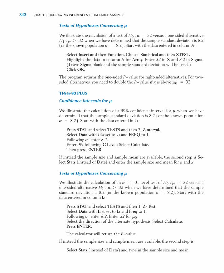
Tests of Hypotheses Concerning �
We illustrate the calculation of a test of : m � 32 versus a one-sided alternative: m 32 when we have determined that the sample standard deviation is 8.2
(or the known population s 8.2). Start with the data entered in column A.
Select Insert and then Function. Choose Statistical and then ZTEST.Highlight the data in column A for Array. Enter 32 in X and 8.2 in Sigma.(Leave Sigma blank and the sample standard deviation will be used.)Click OK.
The program returns the one-sided P–value for right-sided alternatives. For two-sided alternatives, you need to double the P–value if is above � 32.
TI-84/-83 PLUS
Confidence Intervals for �
We illustrate the calculation of a 99% confidence interval for m when we havedetermined that the sample standard deviation is 8.2 (or the known populations 8.2). Start with the data entered in L1.
Press STAT and select TESTS and then 7: Zinterval.Select Data with List set to L1 and FREQ to 1.Following s : enter 8.2.Enter .99 following C-Level: Select Calculate.Then press ENTER.
If instead the sample size and sample mean are available, the second step is Se-lect Stats (instead of Data) and enter the sample size and mean for n and .
Tests of Hypotheses Concerning �
We illustrate the calculation of an a .01 level test of : m � 32 versus aone-sided alternative : m 32 when we have determined that the samplestandard deviation is 8.2 (or the known population s 8.2). Start with thedata entered in column L1.
Press STAT and select TESTS and then 1: Z - Test.Select Data with List set to L1 and Freq to 1.Following s : enter 8.2. Enter 32 for .Select the direction of the alternate hypothesis. Select Calculate.Press ENTER.
The calculator will return the P–value.
If instead the sample size and sample mean are available, the second step is
Select Stats (instead of Data) and type in the sample size and mean.
m0
�H1
H0�
x
�
m0x
�H1
H0
342 CHAPTER 8/DRAWING INFERENCES FROM LARGE SAMPLES
c08.qxd 10/15/09 11:09 AM Page 342

6. REVIEW EXERCISES
6. REVIEW EXERCISES 343
8.78 Refer to Exercise 2.4 where the number of au-tomobile accidents reported per month wererecorded for an intersection. The sample size isn = 59, = 1.949, and s = 1.558 accidents.
(a) Give a point estimate of m , the mean num-ber of accidents reported per month.
(b) Determine the estimated standard error.
(c) Calculate the 98% error margin.
8.79 A student in a large lecture section asked stu-dents how much they paid for a used copy ofthe text. The n = 38 responses yielded
� 3230.84 dollars �
(a) Give a point estimate of m , the meanprice paid.
(b) Determine the estimated standard error.
(c) Calculate the 95% error margin.
8.80 The time it takes for a taxi to drive from theoffice to the airport was recorded on 40 occa-sions. It was found that minutes and
minutes. Give
(a) An estimate of m � population meantime to drive.
(b) An approximate 95.4% error margin.
8.81 By what factor should the sample size be increased to reduce the standard error of to
(a) one-half its original value?
(b) one-fourth its original value?
8.82 A food service manager wants to be 95% cer-tain that the error in the estimate of the meannumber of sandwiches dispensed over thelunch hour is 10 or less. What sample sizeshould be selected if a preliminary samplesuggests
(a) s � 40?
(b) s � 80?
8.83 A zoologist wishes to estimate the meanblood sugar level of a species of animal when
X
s � 5x � 47
x )
2 � 2028.35( xi�� xi
x
injected with a specified dosage of adrenaline.A sample of 55 animals of a common breedare injected with adrenaline, and their bloodsugar measurements are recorded in units ofmilligrams per 100 milliliters of blood. Themean and standard deviation of these mea-surements are found to be 126.9 and 10.5,respectively.
(a) Give a point estimate of the popula-tion mean and find a 95.4% error margin.
(b) Determine a 90% confidence interval forthe population mean.
8.84 Refer to Exercise 2.3 and the data on the num-ber of extracurricular activities in which 30students participated in the past week. Thesedata have
(a) Obtain a 98% confidence interval for m ,the population mean number of activities.
(b) In a long series of experiments, each in-volving different students, what propor-tion of the intervals would cover m?
8.85 After feeding a special diet to 80 mice, the sci-entist measures their weight in grams and ob-tains grams and grams. Hestates that a 90% confidence interval for m isgiven by
or ( 34.26, 35.74 )
(a) Was the confidence interval calculated cor-rectly? If not, provide the correct result.
(b) Does the interval (34.26, 35.74) coverthe true mean? Explain your answer.
8.86 The amount of PCBs was measured in 40 sam-ples of soil that were treated with contami-nated sludge. The following summary statisticswere obtained.
s = .5 p.p.mx = 3.56
� 35 � 1.645 4
√80 , 35 � 1.645
4
√80 �
s � 4x � 35
s � 1.607 activitiesx � 1.925n � 30
c08.qxd 10/15/09 11:09 AM Page 343

(a) Perform a test of hypotheses with the in-tent of establishing that the mean PCBcontamination is less than 3.7 p.p.m. Takea = .05.
(b) What error could you have possibly madein Part(a)?
8.87 In each case, identify the null hypothesis ( )and the alternative hypothesis ( ) using theappropriate symbol for the parameter of interest.
(a) A consumer group plans to test-drive sev-eral cars of a new model in order to docu-ment that its average highway mileage isless than 50 miles per gallon.
(b) Confirm the claim that the mean numberof pages per transmission sent by a cam-pus fax station is more than 3.4.
(c) A chiropractic method will be tried on anumber of persons suffering from persistentbackache in order to demonstrate the claimthat its success rate is higher than 50%.
(d) The setting of an automatic dispenserneeds adjustment when the mean fill dif-fers from the intended amount of 16ounces. Several fills will be accuratelymeasured in order to decide if there is aneed for resetting.
(e) The content of fat in a gourmet chocolateice cream is more than the amount, 4%,that is printed on the label.
8.88 A literary critic wants to establish that the meannumber of words per sentence, appearing in anewly discovered short story, is different from9.1 words.A sample of 36 sentences provided the data
and s = 1.2
(a) Formulate the null and alternative hypothe-ses. (Define any symbols you use.)
(b) Determine the test statistic.
(c) Give the form of the rejection region.
(d) What is the conclusion to your test? Takea = .10.
(e) Calculate a P–value.
(f) Based on Part (d), what error could youhave possibly made?
x = 8.6
H1
H0
344 CHAPTER 8/DRAWING INFERENCES FROM LARGE SAMPLES
8.89 A test will be conducted to see how long aseven-ounce tube of toothpaste lasts. The re-searcher wants to establish that the mean timeis greater than 30.5 days. From a random sam-ple of size 75, an investigator obtains and s = 6.2 days.
(a) Formulate the null and alternative hy-potheses. (Define any symbols you use.)
(b) Determine the test statistic.
(c) Give the form of the rejection region.
(d) What is the conclusion to your test? Takea = .10.
(e) Calculate a P– value.
(f) Based on Part (d), what error could youhave possibly made?
8.90 In a given situation, suppose was rejectedat a � .05. Answer the following questions as“yes,” “no,” or “can’t tell” as the case may be.
(a) Would also be rejected at a � .03?
(b) Would also be rejected at a � .10?
(c) Is the P–value larger than .05?
8.91 Refer to the data on the amount of reflectedlight from urban areas in Table D.3b of theData Bank. A computer calculation for a testof : m � 84 versus : m � 84 has theoutput
Test of mu = 84 vs mu not = 84
Variable N Mean StDevLighturb 40 82.075 4.979
Variable Z PLighturb -2.45 0.014
(a) What is the conclusion of the test when a � .03?
(b) Use the value for Z to test the null hy-pothesis : m � 84 versus the one-sided alternative : m � 84 at the a �.01 level of significance.
8.92 A company wishing to improve its customerservice collected hold times from 75 randomlyselected incoming calls to its hot line that wereput on hold. These calls had sample mean holdtime minutes and minutes.s � 2.3x � 3.4
H0
H0
H1H0
H0
H0
H0
x = 32.3
c08.qxd 10/15/09 11:09 AM Page 344

Obtain a 99% confidence interval for m , thepopulation mean hold time.
8.93 The daily number of kayaks sold, X, at a watersports store has the probability distribution
x 0 1 2
f (x ) .5 .3 .2
(a) Find the expected number of kayaks soldin a day.
(b) Find the standard deviation of the num-ber of kayaks sold in a day.
(c) Suppose data from the next 64 differentdays give and standard devia-tion s � .40 number of kayaks sold. Canwe conclude that the mean number ofkayaks sold is greater than it used to be?Test with a � .05.
8.94 In a large-scale, cost-of-living survey under-taken last January, weekly grocery expenses forfamilies with one or two children were foundto have a mean of $148 and a standard devia-tion of $25. To investigate the current situation,a random sample of families with one or twochildren is to be chosen and their last week’sgrocery expenses are to be recorded.
(a) How large a sample should be taken if onewants to be 95% sure that the error of esti-mation of the population mean grocery ex-penses per week for families with one ortwo children does not exceed $2? (Use theprevious s as an estimate of the current s. )
(b) A random sample of 100 families is actu-ally chosen, and from the data of theirlast week’s grocery bills, the mean and thestandard deviation are found to be $155and $22, respectively. Construct a 98%confidence interval for the current meangrocery expense per week for the popula-tion of families with one or two children.
8.95 A random sample of 2000 persons from the la-bor force of a large city are interviewed, and175 of them are found to be unemployed.
(a) Estimate the rate of unemployment basedon the data.
(b) Establish a 95% error margin for your es-timate.
x � .84
6. REVIEW EXERCISES 345
8.96 Referring to Exercise 8.95, compute a 98% con-fidence interval for the rate of unemployment.
8.97 Out of a sample of n = 625 students interviewed,139 had missed at least one class last week.Obtain a 95% confidence interval for p = pro-portion of all students that missed at least oneclass last week.
8.98 With reference to Exercise 8.97, conduct a testwith the intent of establishing that p > .20.
(a) Formulate the null and alternative hy-potheses.
(b) Determine the test statistic.
(c) Give the form of the rejection region.
(d) What is the conclusion to your test? Takea = .05.
(e) Calculate a P–value.
(f) Based on Part (d), what error could youhave possibly made?
8.99 From July 1 through August 15, 2008, UnitedAirlines flew 137 flights from Chicago, Illinois,to Austin, Texas. Of these, 44 arrived late. Treatthis as a random sample and conduct a test withthe intent of establishing that the populationproportion of late flights is greater than .25.
(a) Formulate the null and alternative hypothe-ses. Define any symbols.
(b) Determine the test statistic.
(c) Give the form of the rejection region.
(d) What is the conclusion to your test? Takea = .05.
(e) Calculate a P–value.
(f) Based on Part (d), what error could youhave possibly made?
8.100 Each year, an insurance company reviews itsclaim experience in order to set future rates.Regarding their damage-only automobile in-surance policies, at least one claim was madeon 2073 of the 12,299 policies in effect for theyear. Treat these data as a random sample forthe population of all possible damage-onlypolicies that could be issued.
(a) Test, at level a � .05, the null hypothesisthat the probability of at least one claim is0.16 versus a two-sided alternative.
c08.qxd 10/15/09 11:09 AM Page 345

(b) Calculate the P–value and comment onthe strength of evidence.
8.101 A genetic model suggests that 80% of theplants grown from a cross between two givenstrains of seeds will be of the dwarf variety. Af-ter breeding 200 of these plants, 136 were ob-served to be of the dwarf variety.
(a) Does this observation strongly contradictthe genetic model?
(b) Construct a 95% confidence interval forthe true proportion of dwarf plants ob-tained from the given cross.
*8.102 Finding the power of a test. Consider theproblem of testing : m � 10 versus
: m 10 with n � 64, s � 2 (known),and a � .025. The rejection region of thistest is given by
Suppose we wish to calculate the power of thistest at the alternative � 11. Power �the probability of rejecting the null hypothesiswhen the alternative is true. Since our test re-jects the null hypothesis when itspower at � 11 is the probability
when the true mean � 11]
If the population mean is 11, we know that has the normal distribution with mean 11 andsd � The stan-dardized variable is
and we calculate
(using normal table)
Following the above steps, calculate the powerof this test at the alternative:
� P [ Z � �2.04] � .9793
� P �Z �10.49 � 11
.25 �
Power � P [ X � 10.49 when �1 � 11]
Z �X � 11
.25
� / √n � 2/√64 � .25.
X
m1P[ X � 10.49
m1
� 10.49,X
m1
R : X � 10 � 1.96 2
√64� 10.49
R : X � 10
2 / √64� 1.96 or
H1
H0
346 CHAPTER 8/DRAWING INFERENCES FROM LARGE SAMPLES
(a) � 10.5
(b) � 10.8
8.103 Refer to the data on the computer attitudescore (CAS) in Table D.4 of the Data Bank. Acomputer summary of a level a � .05 test of
: m � 2.6 versus a two-sided alternativeand a 95% confidence interval is given below.
One-Sample Z: CAS
Test of mu = 2.6 vs mu not = 2.6
Variable N Mean StDevCAS 35 2.8157 0.4840
Variable 95.0% CI Z PCAS ( 2.6554, 2.9761) 2.64 0.008
(a) Will the 99% confidence interval formean CAS be smaller or larger than theone in the printout? Verify your answerby determining the 99% confidence in-terval.
(b) Use the value for Z to test the null hypoth-esis : m � 2.6 versus the one-sidedalternative : m 2.6 at the a � .05level of significance.
8.104 Refer to the data on percent malt extract inTable D.8 of the Data Bank. A computer sum-mary of a level a � .05 test of : m � 77versus a two-sided alternative and a 95% confi-dence interval is given below.
One-Sample Z: malt extract(%)
Test of mu = 77 vs mu not = 77
Variable N Mean StDev
malt extract 40 77.458 1.101
Variable 95.0% CI Z P
malt extract ( 77.116, 77.799) 2.63 0.009
(a) Will the 98% confidence interval formean malt extract be smaller or largerthan the one in the printout? Verify youranswer by determining the 98% confi-dence interval.
( b) Use the value for Z to test the nullhypothesis : m � 77.0 versus theH0
H0
H1
H0
H0
m1
m1
c08.qxd 10/15/09 11:09 AM Page 346

one-sided alternative : m 77.0 atthe a � .05 level of significance.
The Following Exercises Require a Computer
8.105 Refer to the data on the heights of red pineseedlings in Exercise 8.4. Use MINITAB (orsome other package program) to:
(a) Find a 97% percent confidence intervalfor the mean height.
(b) Test : m � 1.9 versus : m � 1.9centimeters with a � .03.
8.106 Referring to speedy lizard data in Exercise2.19, page 38, obtain a 95% confidence inter-val for the mean speed of that genus.
8.107 Refer to the male salmon data given in TableD.7 of the Data Bank. Use MINITAB or someother package program to find a 90% largesample confidence interval for the mean fresh-water growth.
8.108 Refer to the physical fitness data given in TableD.5 of the Data Bank. Use MINITAB or someother package program to:
H1H0
H1
6. REVIEW EXERCISES 347
(a) Find a 97% large sample confidence inter-val for the pretest number of situps.
(b) Construct a histogram to determine if theunderlying distribution is symmetric orhas a long tail to one side.
8.109 Refer to the sleep data given in Table D.10 ofthe Data Bank. Use MINITAB or some otherpackage program to:
(a) Find a 95% large sample confidenceinterval for the mean number of breath-ing pauses per hour (BPH).
(b) Construct a histogram to determine if theunderlying distribution is symmetric orhas a long tail to one side.
8.110 Refer to the grizzly bear data given in Table D.8of the Data Bank. Use MINITAB or someother package program to:
(a) Find a 95% large sample confidenceinterval for the mean weight in pounds ofall bears living in that area.
(b) Construct a histogram to determine if theunderlying distribution is symmetric orhas a long tail to one side.
c08.qxd 10/15/09 11:09 AM Page 347

c08.qxd 10/15/09 11:09 AM Page 348

1. Introduction2. Student’s t Distribution3. Inferences About m—Small Sample Size4. Relationship between Tests and Confidence Intervals5. Inferences about the Standard Deviation s
(The Chi-Square Distribution)6. Robustness of Inference Procedures7. Review Exercises
9
Small Sample Inferences for Normal Populations
c09.qxd 10/15/09 11:10 AM Page 349

Collecting a Sample of Lengths of Anacondas
Jesus Rivas, a herpetologist, is currently doing the definitive research on greenanacondas. These snakes, some of the largest in the world, can grow to 25 feet inlength. They have been known to swallow live goats and even people. JesusRivas and fellow researchers walk barefoot in shallow water in the Llanos grass-lands shared by Venezuela and Colombia during the dry season. When they feela snake with their feet, they grab and hold it with the help of another person.After muzzling the snake with a sock and tape, they place a string along animaginary centerline from head to tail. The measured length of string is therecorded length of the anaconda.
Females are typically larger than males. The lengths (feet) of 21 females are
10.2 11.4 13.6 17.1 16.5 11.8 15.611.8 11.3 11.9 9.6 14.4 13.2 13.512.4 12.1 11.6 8.6 13.0 16.3 14.4
If the captured snakes can be treated as a random sample, a 95% confidence in-terval for the mean length of a female anaconda in that area is given in the com-puter output
One-Sample T: Length(ft)
Variable N Mean StDev 95.0% CILength(ft) 21 12.871 2.262 ( 11.842, 13.901)
Both capturing and measuring make data collection difficult.© Gary Braasch/The Image Bank/Getty Images
c09.qxd 10/15/09 11:10 AM Page 350

1. INTRODUCTION
In Chapter 8, we discussed inferences about a population mean when a largesample is available. Those methods are deeply rooted in the central limit theo-rem, which guarantees that the distribution of is approximately normal. Bythe versatility of the central limit theorem, we did not need to know the specificform of the population distribution.
Many investigations, especially those involving costly experiments, requirestatistical inferences to be drawn from small samples (n � 30, as a rule ofthumb). Since the sample mean will still be used for inferences about m, wemust address the question, “What is the sampling distribution of when n isnot large?” Unlike the large sample situation, here we do not have an unquali-fied answer. In fact, when n is small, the distribution of does depend to a con-siderable extent on the form of the population distribution. With the centrallimit theorem no longer applicable, more information concerning the popula-tion is required for the development of statistical procedures. In other words,the appropriate methods of inference depend on the restrictions met by thepopulation distribution.
In this chapter, we describe how to set confidence intervals and test hy-potheses when it is reasonable to assume that the population distribution isnormal.
We begin with inferences about the mean m of a normal population. Guidedby the development in Chapter 8, it is again natural to focus on the ratio
when s is also unknown. The sampling distribution of this ratio, called Student’st distribution, is introduced next.
2. STUDENT’S t DISTRIBUTION
When is based on a random sample of size n from a normal N (m, s ) popula-tion, we know that is exactly distributed as N (m, s / Consequently, thestandardized variable
has the standard normal distribution.Because s is typically unknown, an intuitive approach is to estimate s by
the sample standard deviation S. Just as we did in the large sample situation, weconsider the ratio
T �X � �
S / √n
Z �X � �
� / √n
√n ).XX
X � �
S / √n
X
XX
X
2. STUDENT’S t DISTRIBUTION 351
c09.qxd 10/15/09 11:10 AM Page 351

Its probability density function is still symmetric about zero. Although estimat-ing s with S does not appreciably alter the distribution in large samples, it doesmake a substantial difference if the sample is small. The new notation T is re-quired in order to distinguish it from the standard normal variable Z. In fact,this ratio is no longer standardized. Replacing s by the sample quantity S intro-duces more variability in the ratio, making its standard deviation larger than 1.
The distribution of the ratio T is known in statistical literature as “Student’st distribution.” This distribution was first studied by a British chemist W. S.Gosset, who published his work in 1908 under the pseudonym “Student.” Thebrewery for which he worked apparently did not want the competition to knowthat it was using statistical techniques to better understand and improve its fer-mentation process.
The qualification “with n � 1 degrees of freedom” is necessary, becausewith each different sample size or value of n � 1, there is a different t distribu-tion. The choice n � 1 coincides with the divisor for the estimator that isbased on n � 1 degrees of freedom.
The t distributions are all symmetric around 0 but have tails that are morespread out than the N (0, 1) distribution. However, with increasing degrees offreedom, the t distributions tend to look more like the N (0, 1) distribution.This agrees with our previous remark that for large n the ratio
is approximately standard normal. The density curves for t with 2 and 5 degreesof freedom are plotted in Figure 1 along with the N (0, 1) curve.
Appendix B, Table 4, gives the upper a points for some selected values ofa and the degrees of freedom (abbreviated d.f.).
The curve is symmetric about zero so the lower a point is simply � . Theentries in the last row marked “d.f. � infinity” in Appendix B, Table 4, are ex-actly the percentage points of the N (0, 1) distribution.
t�
t�
X � �
S / √n
S2
352 CHAPTER 9/SMALL SAMPLE INFERENCES FOR NORMAL POPULATIONS
Student’s t Distribution
If , . . . , is a random sample from a normal population N (m, s )and
then the distribution of
is called Student’s t distribution with n � 1 degrees of freedom
T �X � �
S / √n
X �1n
� Xi and S2 ��
( Xi � X
)2
n � 1
XnX1
c09.qxd 10/15/09 11:10 AM Page 352
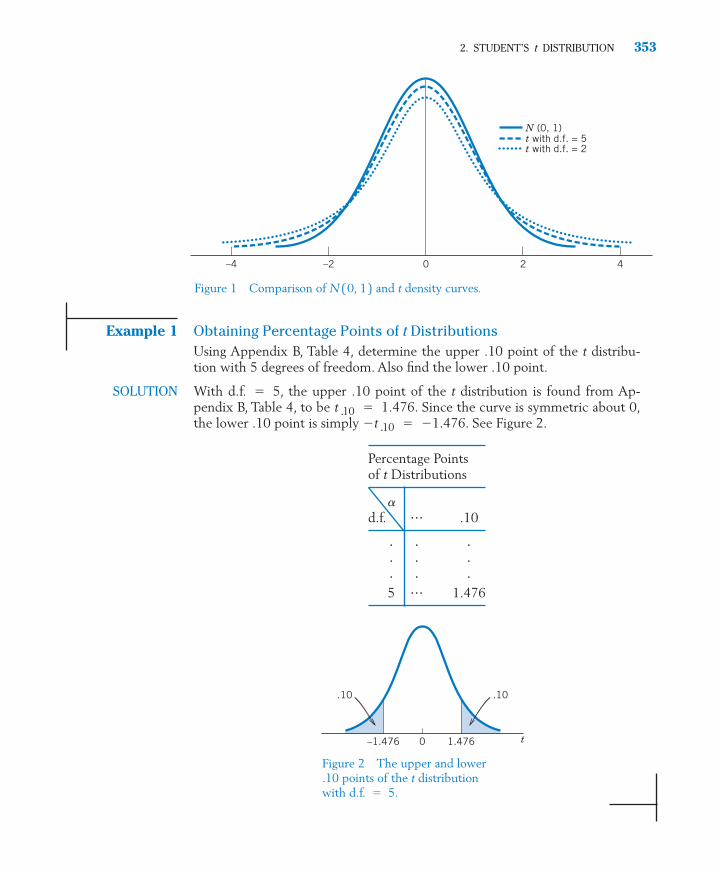
Example 1 Obtaining Percentage Points of t DistributionsUsing Appendix B, Table 4, determine the upper .10 point of the t distribu-tion with 5 degrees of freedom. Also find the lower .10 point.
SOLUTION With d.f. � 5, the upper .10 point of the t distribution is found from Ap-pendix B, Table 4, to be � 1.476. Since the curve is symmetric about 0,the lower .10 point is simply � � �1.476. See Figure 2.t .10
t .10
2. STUDENT’S t DISTRIBUTION 353
–4 –2 0 2
N (0, 1)t with d.f. = 5t with d.f. = 2
4
0 1.476–1.476
.10.10
t
Figure 1 Comparison of N (0, 1) and t density curves.
Figure 2 The upper and lower .10 points of the t distribution with d.f. � 5.
Percentage Points of t Distributions
a
d.f. ��� .10
� � �� � �� � �5 ��� 1.476
c09.qxd 10/15/09 11:10 AM Page 353

Example 2 Determining a Central Interval Having Probability .90For the t distribution with d.f. � 9, find the number b such that
SOLUTION In order for the probability in the interval (�b, b ) to be .90, we must have aprobability of .05 to the right of b and, correspondingly, a probability of .05to the left of �b (see Figure 3). Thus, the number b is the upper a � .05point of the t distribution. Reading Appendix B, Table 4, at a � .05 and d.f. � 9, we find � 1.833, so b � 1.833.
Exercises
t.05
P [ �b � T � b ] � .90.
354 CHAPTER 9/SMALL SAMPLE INFERENCES FOR NORMAL POPULATIONS
0 b–b
0.050.05
t
Figure 3 Finding the 5th percentile.
.025 .05
0 0 tt
t t0 0
.10.05
.025
d.f. = 19d.f. = 25
d.f. = 18d.f. = 12(a) (b)
(c) (d)
9.1 Using the table for the t distributions, find:
(a) The upper .05 point when d.f. � 5.
(b) The lower .025 point when d.f. � 13.
(c) The lower .01 point when d.f. � 8.
(d) The upper .10 point when d.f. � 11.
9.2 Name the t percentiles shown and find their val-ues from Appendix B, Table 4.
9.3 Using the table for the t distributions find:
(a) The 90th percentile of the t distributionwhen d.f. � 9.
(b) The 99th percentile of the t distributionwhen d.f. � 4.
(c) The 5th percentile of the t distributionwhen d.f. � 22.
(d) The lower and upper quartiles of the t dis-tribution when d.f. � 18.
9.4 Find the probability of
(a) T � �1.761 when d.f. � 14
(b) when d.f. � 8
(c) �1.734 � T � 1.734 when d.f. � 18
(d) �1.812 � T � 2.764 when d.f. � 10
9.5 In each case, find the number b so that
(a) when d.f. � 5
(b) when d.f. � 16
(c) when d.f. � 7
(d) when d.f. � 12P [ T b ] � .99
P [ T b ] � .01
P [ �b � T � b ] � .95
P [ T � b ] � .95
� T � 2.306
c09.qxd 10/15/09 11:10 AM Page 354

9.6 Record the values for d.f. of 5, 10, 15, 20,and 29. Does this percentile increase or decreasewith increasing degrees of freedom?
9.7 Using the table for the t distributions, make anassessment for the probability of the statedevent. (The answer to part (a) is provided.)
(a) T 2.6 when d.f. � 7 ( Answer:is between .01 and .025 be-
cause 2.6 lies between and
(b) when d.f. � 16
(c) when d.f. � 11
(d) when d.f. � 10
(e) when d.f. � 17� T � � 2.8
� T � 1.9
T � �1.5
T 1.9
t.01 � 2.998.)t.05 � 2.365
P [ T 2.6 ]
t.05
3. INFERENCES ABOUT m—SMALL SAMPLE SIZE 355
9.8 What can you say about the number c in eachcase? Justify your answer. (The answer to part(a) is provided.)
(a) when d.f. � 5
(Answer: c is between 2.015 and 2.571 be-cause and
(b) when d.f. � 11
(c) when d.f. � 13
(d) when d.f. � 6
(e) when d.f. � 27P [ � T � � c ] � .96
P [ � T � c ] � .03
P [ T � �c ] � .004
P [ T c ] � .016
t.025 � 2.571.)t.05 � 2.015
P [ T c ] � .03
3. INFERENCES ABOUT �—SMALL SAMPLE SIZE
3.1. CONFIDENCE INTERVAL FOR �
The distribution of
provides the key for determining a confidence interval for �, the mean of a nor-mal population. For a 100(1 � a)% confidence interval, we consult the t table(Appendix B, Table 4) and find , the upper a /2 point of the t distributionwith n � 1 degrees of freedom (see Figure 4).
Since has the t distribution with d.f. � n � 1, we have
� P ��t� / 2S
√n� X � � � t� / 2
S
√n�1 � � � P � �t� / 2 �
X � �
S / √n� t� / 2 �
X � �
S / √n
t� / 2
T �X � �
S / √n
0 t /2
/2
t
α
1 – α
/2α
α–t /2α
Figure 4 and the probabilities.t� /2
c09.qxd 10/15/09 11:10 AM Page 355
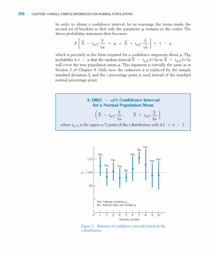
In order to obtain a confidence interval, let us rearrange the terms inside thesecond set of brackets so that only the parameter m remains in the center. Theabove probability statement then becomes
which is precisely in the form required for a confidence statement about m. Theprobability is 1 � a that the random interval to will cover the true population mean m. This argument is virtually the same as inSection 3 of Chapter 8. Only now the unknown s is replaced by the samplestandard deviation S, and the t percentage point is used instead of the standardnormal percentage point.
X t�/2 S / √nX � t�/2 S / √n
P � X � t�/2 S
√n� � � X t�/2
S
√n � � 1 � �
356 CHAPTER 9/SMALL SAMPLE INFERENCES FOR NORMAL POPULATIONS
A 100(1 � �)% Confidence Interval for a Normal Population Mean
where is the upper a/2 point of the t distribution with d.f. � n � 1.t� /2
� X � t�/2 S
√n , X t�/2
S
√n �
Yes
110
= 100µ
90
0 1 2 3 4 5Sample number
Yes: Interval contains .µNo: Interval does not contain .µ
6 7 8 9 10
Yes
Yes
YesNo
Yes
NoYes
Yes Yes
Figure 5 Behavior of confidence intervals based on thet distribution.
c09.qxd 10/15/09 11:10 AM Page 356

Let us review the meaning of a confidence interval in the present context.Imagine that random samples of size n are repeatedly drawn from a normal popula-
tion and the interval calculated in each case.The interval is centered at so the center varies from sample to sample. The lengthof an interval, 2 s/ also varies from sample to sample because it is a mul-tiple of the sample standard deviation s. (This is unlike the fixed-length situation illustrated in Figure 4 of Chapter 8, which was concerned with a known s.) Thus,in repeated sampling, the intervals have variable centers and variable lengths.However, our confidence statement means that if the sampling is repeated many times, about 100(1 � a)% of the resulting intervals would cover the truepopulation mean m.
Figure 5 shows the results of drawing 10 samples of size n � 7 from the normalpopulation with m � 100 and s � 10. Selecting a � .05, we find that the valueof with 6 d.f. is 2.447, so the 95% confidence interval is Inthe first sample, and so the interval is (96.52, 111.24).The95% confidence intervals are shown by the vertical line segments. Nine of 10 cover m.
Example 3 Interpreting a Confidence IntervalThe weights (pounds) of n � 8 female wolves captured in the Yukon-Charley Rivers National Reserve (see Table D.9 of the Data Bank) are
57 84 90 71 77 68 73 71
Treating these weights as a random sample from a normal distribution:(a) Find a 90% confidence interval for the population mean weight of all
female wolves living on the Yukon-Charley Rivers National Reserve.(b) Is m included in this interval?
SOLUTION (a) If we assume that the weights are normally distributed, a 90% confi-dence interval for the mean weight m is given by
where n � 8. The t statistic is based on n � 1 � 8 � 1 � 7 degreesof freedom so, consulting the t table, we find � 1.895. Beforehand,this is a random interval.
To determine the confidence interval from the given sample, we firstobtain the summary statistics
s � √101.268 � 10.063
x– �591.000
8� 73.875 s2 �
708.8757
� 101.268 so
t.05
� X � t.05 S
√n, X � t.05
S
√n �
s � 7.96,x � 103.88X � 2.447S / √7.t.025
√n,t�/2
x( x � t� /2 s / √n, x t� /2 s / √n )
3. INFERENCES ABOUT m—SMALL SAMPLE SIZE 357
c09.qxd 10/15/09 11:10 AM Page 357

The 90% confidence interval for m is then
We are 90% confident that the mean weight of all female wolves isbetween 67.13 and 80.62 pounds. We have this confidence because,over many occasions of sampling, approximately 90% of the inter-vals calculated using this procedure will contain the true mean.
(b) We will never know if a single realization of the confidence interval,such as (67.13, 80.62), covers the unknown m. It is unknown be-cause it is based on every female wolf in the very large reserve. Ourconfidence in the method is based on the high percentage of timesthat m is covered by intervals in repeated samplings.
Remark: When repeated independent measurements are made on the samematerial and any variation in the measurements is basically due to experimen-tal error (possibly compounded by nonhomogeneous materials), the normalmodel is often found to be appropriate. It is still necessary to graph the indi-vidual data points ( too few here) in a dot diagram and normal-scores plot toreveal any wild observations or serious departures from normality. In all smallsample situations, it is important to remember that the validity of a confidenceinterval rests on the reasonableness of the model assumed for the population.
Recall from the previous chapter that the length of a 100(1 � a)% confi-dence interval for a normal m is 2 s / when s is known, whereas it is
2 S / when s is unknown. Given a small sample size n and consequentlya small number of degrees of freedom (n � 1), the extra variability caused byestimating s with S makes the t percentage point much larger than the nor-mal percentage point . For instance, with d.f. � 4, we have � 2.776,which is considerably larger than � 1.96. Thus, when s is unknown, theconfidence estimation of m based on a very small sample size is expected to pro-duce a much less precise inference (namely, a wide confidence interval ) com-pared to the situation when s is known. With increasing n, s can be more closelyestimated by S and the difference between and tends to diminish.
3.2. HYPOTHESES TESTS FOR �
The steps for conducting a test of hypotheses concerning a population mean werepresented in the previous chapter. If the sample size is small, basically the sameprocedure can be followed provided it is reasonable to assume that the populationdistribution is normal. However, in the small sample situation, our test statistic
has Student’s t distribution with n � 1 degrees of freedom.
T �X � � 0
S / √n
z� /2t� /2
z.025
t.025z� /2
t� /2
√nt� /2
√nz� /2
73.875 � 1.895 �10.063
√8� 73.875 � 6.742 or ( 67.13, 80.62 )
358 CHAPTER 9/SMALL SAMPLE INFERENCES FOR NORMAL POPULATIONS
c09.qxd 10/15/09 11:10 AM Page 358

The t table (Appendix B, Table 4) is used to determine the rejection regionto test hypotheses about �.
Example 4 A Student’s t Test to Confirm the Water Is SafeA city health department wishes to determine if the mean bacteria count perunit volume of water at a lake beach is within the safety level of 200. A re-searcher collected 10 water samples of unit volume and found the bacteriacounts to be
175 190 205 193 184207 204 193 196 180
Do the data strongly indicate that there is no cause for concern? Test with a � .05.
SOLUTION Let m denote the current (population) mean bacteria count per unit volumeof water. Then, the statement “no cause for concern” translates to m � 200,and the researcher is seeking strong evidence in support of this hypothesis. Sothe formulation of the null and alternative hypotheses should be
Since the counts are spread over a wide range, an approximation by a contin-uous distribution is not unrealistic for inference about the mean. Assumingfurther that the measurements constitute a sample from a normal popula-tion, we employ the t test with
T �X � 200
S / √10 d.f. � 9
H0 : � � 200 versus H1 : � � 200
3. INFERENCES ABOUT m—SMALL SAMPLE SIZE 359
Hypotheses Tests for �—Small Samples
To test : m � m concerning the mean of a normal population, thetest statistic is
which has Student’s t distribution with n � 1 degrees of freedom:
The test is called a Student’s t test or simply a t test.
H1: � �0 R : � T � � t�/2
H1: � � �0 R : T � �t�
H1: � � 0 R : T � t�
T �X � �0
S / √n
0H0
c09.qxd 10/15/09 11:10 AM Page 359

We test at the level of significance a � .05. Since is left-sided, we set therejection region T � � . From the t table we find that with d.f. � 9is 1.833, so our rejection region is R�T � �1.833 as in Figure 6. Computa-tions from the sample data yield
Because the observed value t � �2.14 is smaller than �1.833, the null hy-pothesis is rejected at a � .05. On the basis of the data obtained from these10 measurements, there does seem to be strong evidence that the true meanis within the safety level.
Values of T smaller than �2.14 are more extreme evidence in favor ofthe alternative hypothesis. Since, with 9 degrees of freedom, � 1.833and � 2.262, the P–value is between .05 and .025. The accompanyingcomputer output gives
There is strong evidence that the mean bacteria count is within the safety level.
P–value � P [ T � �2.14 ] � .031 ( see Figure 7 )
t.025
t.05
t �192.7 � 200
10.81 / √10�
�7.33.418
� �2.14
s � 10.81
x � 192.7
t.05t.05
H1
360 CHAPTER 9/SMALL SAMPLE INFERENCES FOR NORMAL POPULATIONS
0–1.833 t
.05
0–2.14 t
.031
Figure 6 Left-sided rejection region.T � �1.833
Figure 7 P–value for left-sided rejection region, T statistic.
Computer Solution to Example 4
(see the Techology section for the MINITAB COMMANDS)
T Test of the Mean
Test of mu � 200.00 vs mu � 200.00
Variable N Mean StDev SE Mean T P
Bac Coun 10 192.70 10.81 3.42 �2.14 0.031
c09.qxd 10/15/09 11:10 AM Page 360
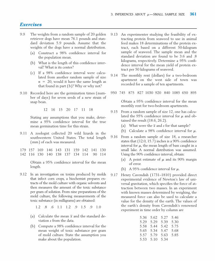
9.9 The weights from a random sample of 20 goldenretriever dogs have mean 76.1 pounds and stan-dard deviation 5.9 pounds. Assume that theweights of the dogs have a normal distribution.
(a) Construct a 98% confidence interval forthe population mean.
(b) What is the length of this confidence inter-val? What is its center?
(c) If a 98% confidence interval were calcu-lated from another random sample of sizen � 20, would it have the same length asthat found in part (b)? Why or why not?
9.10 Recorded here are the germination times (num-ber of days) for seven seeds of a new strain ofsnap bean.
12 16 15 20 17 11 18
Stating any assumptions that you make, deter-mine a 95% confidence interval for the truemean germination time for this strain.
9.11 A zoologist collected 20 wild lizards in thesouthwestern United States. The total length(mm) of each was measured.
179 157 169 146 143 131 159 142 141 130142 116 130 140 138 137 134 114 90 114
Obtain a 95% confidence interval for the meanlength.
9.12 In an investigation on toxins produced by moldsthat infect corn crops, a biochemist prepares ex-tracts of the mold culture with organic solvents andthen measures the amount of the toxic substanceper gram of solution. From nine preparations of themold culture, the following measurements of thetoxic substance (in milligrams) are obtained:
1.2 .8 .6 1.1 1.2 .9 1.5 .9 1.0
(a) Calculate the mean and the standard de-viation s from the data.
(b) Compute a 98% confidence interval for themean weight of toxic substance per gramof mold culture. State the assumption youmake about the population.
x
3. INFERENCES ABOUT m—SMALL SAMPLE SIZE 361
Exercises
9.13 An experimenter studying the feasibility of ex-tracting protein from seaweed to use in animalfeed makes 18 determinations of the protein ex-tract, each based on a different 50-kilogramsample of seaweed. The sample mean and thestandard deviation are found to be 3.6 and .8kilograms, respectively. Determine a 95% confi-dence interval for the mean yield of protein ex-tract per 50 kilograms of seaweed.
9.14 The monthly rent (dollars) for a two-bedroomapartment on the west side of town wasrecorded for a sample of ten apartments.
950 745 875 827 1030 920 840 1085 650 895
Obtain a 95% confidence interval for the meanmonthly rent for two-bedroom apartments.
9.15 From a random sample of size 12, one has calcu-lated the 95% confidence interval for m and ob-tained the result (18.6, 26.2).(a) What were the and s for that sample?(b) Calculate a 98% confidence interval for m.
9.16 From a random sample of size 18, a researcherstates that (12.0, 15.7) inches is a 90% confidenceinterval for m, the mean length of bass caught in asmall lake. A normal distribution was assumed.Using the 90% confidence interval, obtain:(a) A point estimate of m and its 90% margin
of error.(b) A 95% confidence interval for m.
9.17 Henry Cavendish (1731–1810) provided directexperimental evidence of Newton’s law of uni-versal gravitation, which specifies the force of at-traction between two masses. In an experimentwith known masses determined by weighing, themeasured force can also be used to calculate avalue for the density of the earth. The values ofthe earth’s density from Cavendish’s renownedexperiment in time order by column are
5.36 5.62 5.27 5.465.29 5.29 5.39 5.305.58 5.44 5.42 5.755.65 5.34 5.47 5.685.57 5.79 5.63 5.855.53 5.10 5.34
x
c09.qxd 10/15/09 11:10 AM Page 361

[These data were published in PhilosophicalTransactions, 17 (1798), p. 469.] Find a 99%confidence interval for the density of the earth.
9.18 Refer to Exercise 9.14. Do these data supportthe claim that the mean monthly rent for a two-bedroom apartment differs from 775 dollars?Take a � .05.
9.19 Refer to Exercise 9.14. Do these data providestrong evidence for the claim that the monthlyrent for a two-bedroom apartment is greaterthan 800 dollars? Take a � .05.
9.20 In a lake pollution study, the concentration of lead in the upper sedimentary layer of a lake bottom is measured from 25 sediment samples of 1000 cubic centimeters each. Thesample mean and the standard deviation of the measurements are found to be .38 and .06,respectively. Compute a 99% confidence intervalfor the mean concentration of lead per 1000 cubic centimeters of sediment in the lake bottom.
9.21 The data on the lengths of anacondas on thefront piece of the chapter yield a 95% confi-dence interval for the population mean length ofall anaconda snakes in the area of the study.
Variable N Mean StDev 95.0% CI
Length(ft) 21 12.871 2.262 ( 11.842, 13.901)
(a) Is the population mean length of all femaleanacondas living in the study area con-tained in this interval?
(b) Explain why you are 95% confident that itis contained in the interval.
9.22 Refer to the data on the weight (pounds) ofmale wolves given in Table D.9 of the DataBank. A computer calculation gives a 95% confi-dence interval.
Variable N Mean StDev 95.0% CI
Malewt 11 91.91 12.38 ( 83.59, 100.23)
(a) Is the population mean weight for all malewolves in the Yukon-Charley RiversNational Reserve contained in this interval?
(b) Explain why you are 95% confident that itis contained in the interval.
362 CHAPTER 9/SMALL SAMPLE INFERENCES FOR NORMAL POPULATIONS
9.23 The following measurements of the diameters(in feet) of Indian mounds in southern Wisconsinwere gathered by examining reports in WisconsinArcheologist (courtesy of J. Williams).
22 24 24 30 22 20 28 30 24 34 36 15 37
(a) Do these data substantiate the conjecturethat the population mean diameter is largerthan 21 feet? Test at a � .01.
(b) Determine a 90% confidence interval for thepopulation mean diameter of Indian mounds.
9.24 Measurements of the acidity (pH) of rain sampleswere recorded at 13 sites in an industrial region.
3.5 5.1 5.0 3.6 4.8 3.6 4.74.3 4.2 4.5 4.9 4.7 4.8
Determine a 95% confidence interval for themean acidity of rain in that region.
9.25 Refer to Exercise 9.11, where a zoologist col-lected 20 wild lizards in the southwesternUnited States. Do these data substantiate aclaim that the mean length is greater than 128mm? Test with a � .05.
9.26 Geologists dating rock, using a strontium-isotopetechnique, provided the ages 5.2 and 4.4 millionyears for two specimens. Treating these as a ran-dom sample of size 2 from a normal distribution
(a) Obtain a 90% confidence interval for m thetrue age of the rock formation.
(b) Geologists do get an estimate of error fromthe strontium-isotope analysis so they usu-ally do not take duplicate readings. From astatistical point of view, two observations aremuch better than one. What happens to thelength of the confidence interval if the sam-ple size were increased from 2 to 4? Answerby considering the ratio of the lengths.
9.27 The data on the weight ( lb) of female wolves,from Table D.9 of the Data Bank, are
57 84 90 71 71 77 68 73
Test the null hypothesis that the mean weight offemales is 83 pounds versus a two-sided alterna-tive. Take a � .05.
9.28 The ability of a grocery store scanner to read ac-curately is measured in terms of maximum atten-uation (db). In one test with 20 different products,the values of this measurement had a mean 10.7
c09.qxd 10/15/09 11:10 AM Page 362
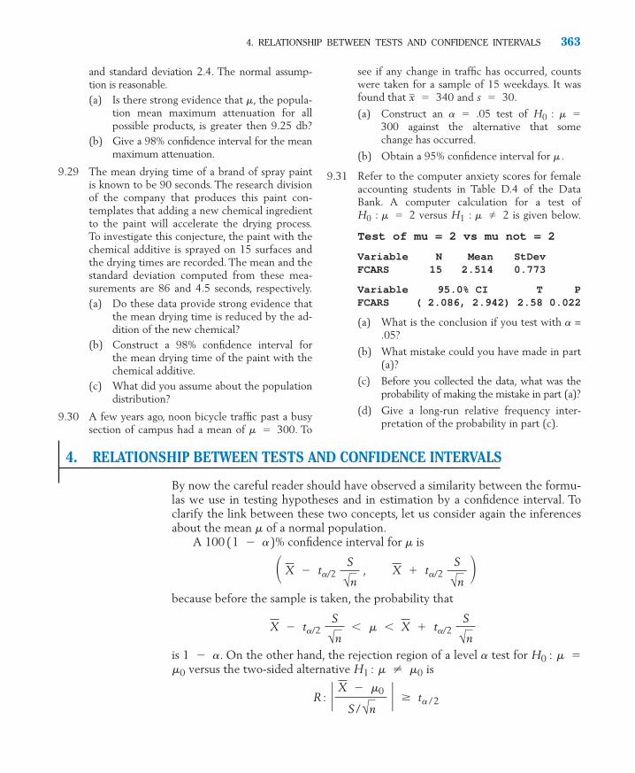
and standard deviation 2.4. The normal assump-tion is reasonable.(a) Is there strong evidence that m, the popula-
tion mean maximum attenuation for allpossible products, is greater then 9.25 db?
(b) Give a 98% confidence interval for the meanmaximum attenuation.
9.29 The mean drying time of a brand of spray paintis known to be 90 seconds. The research divisionof the company that produces this paint con-templates that adding a new chemical ingredientto the paint will accelerate the drying process.To investigate this conjecture, the paint with thechemical additive is sprayed on 15 surfaces andthe drying times are recorded. The mean and thestandard deviation computed from these mea-surements are 86 and 4.5 seconds, respectively.(a) Do these data provide strong evidence that
the mean drying time is reduced by the ad-dition of the new chemical?
(b) Construct a 98% confidence interval forthe mean drying time of the paint with thechemical additive.
(c) What did you assume about the populationdistribution?
9.30 A few years ago, noon bicycle traffic past a busysection of campus had a mean of m � 300. To
4. RELATIONSHIP BETWEEN TESTS AND CONFIDENCE INTERVALS 363
see if any change in traffic has occurred, countswere taken for a sample of 15 weekdays. It wasfound that and
(a) Construct an a � .05 test of : m �300 against the alternative that somechange has occurred.
(b) Obtain a 95% confidence interval for m .
9.31 Refer to the computer anxiety scores for femaleaccounting students in Table D.4 of the DataBank. A computer calculation for a test of
: m � 2 versus : m 2 is given below.
Test of mu = 2 vs mu not = 2
Variable N Mean StDevFCARS 15 2.514 0.773
Variable 95.0% CI T PFCARS ( 2.086, 2.942) 2.58 0.022
(a) What is the conclusion if you test with a =.05?
(b) What mistake could you have made in part(a)?
(c) Before you collected the data, what was theprobability of making the mistake in part (a)?
(d) Give a long-run relative frequency inter-pretation of the probability in part (c).
H1H0
H0
s � 30.x � 340
4. RELATIONSHIP BETWEEN TESTS AND CONFIDENCE INTERVALS
By now the careful reader should have observed a similarity between the formu-las we use in testing hypotheses and in estimation by a confidence interval. Toclarify the link between these two concepts, let us consider again the inferencesabout the mean m of a normal population.
A 100 (1 � a)% confidence interval for m is
because before the sample is taken, the probability that
is 1 � a. On the other hand, the rejection region of a level a test for : m �versus the two-sided alternative : m � is
R : �
X � �0
S / √n � � t� /2
m0H1m0
H0
X � t�/2 S
√n� � � X t�/2
S
√n
� X � t�/2 S
√n , X t�/2
S
√n �
c09.qxd 10/15/09 11:10 AM Page 363

Let us use the name “acceptance region” to mean the opposite (or complement)of the rejection region. Reversing the inequality in R, we obtain
Acceptance region
which can also be written as
Acceptance region
The latter expression shows that any given null hypothesis will be accepted(more precisely, will not be rejected) at level a if lies within the 100(1 � a)%confidence interval. Thus, having established a 100(1 � a )% confidenceinterval for m, we know at once that all possible null hypotheses values lyingoutside this interval will be rejected at level of significance a and all those lyinginside will not be rejected.
Example 5 Relation between a 95% Confidence Interval and Two-Sided a � .05TestA random sample of size n � 9 from a normal population produced themean and the standard deviation Obtain a 95% confidenceinterval for m and also test : m � 8.5 versus : m � 8.5 with a � .05.
SOLUTION A 95% confidence interval has the form
where corresponds to degrees of freedom. Hereand so the interval becomes
Turning now to the problem of testing : m � 8.5, we observe thatthe value 8.5 lies in the 95% confidence interval we have just calculated. Us-ing the correspondence between confidence interval and acceptance region,we can at once conclude that : m � 8.5 should not be rejected at a �.05. Alternatively, a formal step-by-step solution can be based on the test statistic
The rejection region consists of both large and small values.
Rejection region
� X � 8.5
S / √n� � t.025 � 2.306
T �X � 8.5
S / √n
H0
H0
�8.3 � 2.306 1.2
√9, 8.3 2.306
1.2
√9� � (7.4, 9.2)
s � 1.2,x � 8.3n � 1 � 8t.025 � 2.306
�X � t.025 S
√n, X t.025
S
√n�
H1H0
s � 1.2.x � 8.3
m0
m0
m0
X � t�/2 S
√n� �0 � X t�/2
S
√n
�t� / 2 �X � �0
S / √n� t� / 2
364 CHAPTER 9/SMALL SAMPLE INFERENCES FOR NORMAL POPULATIONS
c09.qxd 10/15/09 11:10 AM Page 364

Now the observed value does not fall inthe rejection region, so the null hypothesis : m � 8.5 is not rejected at a � .05. This conclusion agrees with the one we arrived at from the confi-dence interval.
This relationship indicates how confidence estimation and tests of hypothe-ses with two-sided alternatives are really integrated in a common framework. Aconfidence interval statement is regarded as a more comprehensive inferenceprocedure than testing a single null hypothesis, because a confidence intervalstatement in effect tests many null hypotheses at the same time.
Exercises
H0
� t � � √9 � 8.3 � 8.5 � / 1.2 � .5
4. RELATIONSHIP BETWEEN TESTS AND CONFIDENCE INTERVALS 365
9.32 Based on a random sample of tail lengths for15 male kites, an investigator calculates the 95%confidence interval (183.0, 195.0) mm based onthe t distribution. The normal assumption isreasonable.
(a) What is the conclusion of the t test for H0 :m � 190.5 versus : m 190.5?
(b) What is the conclusion if : m � 182.2?
9.33 In Example 3, the 95% confidence interval forthe mean weight of female wolves was found tobe (67.13, 80.62) pounds.
(a) What is the conclusion of testing : m �81 versus : m 81 at level a � .05?
(b) What is the conclusion if : m � 69?
9.34 The petal width (mm) of one kind of iris has anormal distribution. Suppose that, from a ran-dom sample of widths, the t based 90% confi-dence interval for the population mean width is(16.8, 19.6) mm. Answer each question “yes,”“no,” or “can’t tell,” and justify your answer. Onthe basis of the same sample:
(a) Would : m � 20 be rejected in favor of: m 20 at a � .10?
(b) Would : m � 18 be rejected in favor of: m 18 at a � .10?
*(c) Would : m � 17 be rejected in favor of: m 17 at a � .05?
*(d) Would : m � 22 be rejected in favor of: m 22 at a � .01?
9.35 Recorded here are the amounts of decrease inpercent body fat for eight participants in an ex-ercise program over three weeks.
H1
H0
H1
H0
H1
H0
H1
H0
H0
H1
H0
H0
H1
1.8 10.6 �1.2 12.9 15.1 �2.0 6.2 10.8
(a) Construct a 95% confidence interval forthe population mean amount m of decreasein percent body fat over the three-weekprogram.
(b) If you were to test : m � 15 versus : m 15 at a � .05, what would youconclude from your result in part (a)?
(c) Perform the hypothesis test indicated inpart (b) and confirm your conclusion.
9.36 Refer to the data in Exercise 9.35.
(a) Construct a 90% confidence interval for m.
(b) If you were to test : m � 10 versus :m 10 at a � .10, what would youconclude from your result in part (a)?Why?
(c) Perform the hypothesis test indicated inpart (b) and confirm your conclusion.
9.37 Establish the connection between the large sam-ple Z test, which rejects : m � m in favorof : m m , at a � .05, if
and the 95% confidence interval
X � 1.96 S
√n to X 1.96
S
√n
X � �0
S / √n� �1.96
Z �X � �0
S / √n� 1.96 or
0H1
0H0
H1H0
H1H0
c09.qxd 10/15/09 11:10 AM Page 365

366 CHAPTER 9/SMALL SAMPLE INFERENCES FOR NORMAL POPULATIONS
5. INFERENCES ABOUT THE STANDARD DEVIATION �(THE CHI-SQUARE DISTRIBUTION)
Aside from inferences about the population mean, the population variabilitymay also be of interest. Apart from the record of a baseball player’s batting av-erage, information on the variability of the player‘s performance from onegame to the next may be an indicator of reliability. Uniformity is often a crite-rion of production quality for a manufacturing process. The quality control en-gineer must ensure that the variability of the measurements does not exceed aspecified limit. It may also be important to ensure sufficient uniformity of theinputted raw material for trouble-free operation of the machines. In this sec-tion, we consider inferences for the standard deviation s of a population underthe assumption that the population distribution is normal. In contrast to the in-ference procedures concerning the population mean m , the usefulness of themethods to be presented here is extremely limited when this assumption is violated.
To make inferences about , the natural choice of a statistic is its sampleanalog, which is the sample variance,
We take as the point estimator of and its square root S as the point esti-mator of s. To estimate by confidence intervals and test hypotheses, we mustconsider the sampling distribution of . To do this, we introduce a new distri-bution, called the distribution (read “chi-square distribution”), whose formdepends on
Unlike the normal or t distribution, the probability density curve of a distribution is an asymmetric curve stretching over the positive side of the lineand having a long right tail. The form of the curve depends on the value of thedegrees of freedom. A typical curve is illustrated in Figure 8.�2
�2
n � 1.�2
S2
� 2S2
S2 �
�n
i � 1 ( Xi � X )2
n � 1
� 2
� Distribution
Let , . . . , be a random sample from a normal population N (m, s ). Then the distribution of
is called the � distribution with n � 1 degrees of freedom.2
�2 �
�n
i � 1 ( Xi � X )2
�2�
(n � 1) S2
�2
XnX1
2
c09.qxd 10/15/09 11:10 AM Page 366

5. INFERENCES ABOUT THE STANDARD DEVIATION s (THE CHI-SQUARE DISTRIBUTION) 367
α
21 –
�α α
2� 2�
f
α
Figure 8 Probability density curve of a x2 distribution.
Percentage Points of the Distributions (Appendix B, Table 5)
a
d.f. ��� .95 ��� .05
� � �� � �� � �
17 ��� 8.67 ��� 27.59
�2
Appendix B, Table 5, provides the upper a points of distributions for vari-ous values of a and the degrees of freedom. As in both the cases of the t and thenormal distributions, the upper a point denotes the value such thatthe area to the right is a. The lower a point or 100ath percentile, read from thecolumn in the table, has an area 1 � a to the right. For example, thelower .05 point is obtained from the table by reading the column, whereasthe upper .05 point is obtained by reading the column
Example 6 Finding Percentage Points of the � DistributionFind the upper .05 point of the distribution with 17 degrees of freedom.Also find the lower .05 point.
SOLUTION
The upper .05 point is read from the column labeled a � .05. We findfor 17 d.f. The lower .05 point is read from the column a �
.95. We find as the lower .05 point.
The is the basic distribution for constructing confidence intervals for or s. We outline the steps in terms of a 95% confidence interval for . Dividings 2
s 2x2
�.952 � 8.67,
�.052 � 27.59
�2
2
�.052 .
�.952
�1��2
�2��2
�2
c09.qxd 10/15/09 11:10 AM Page 367

the probability a � .05 equally between the two tails of the distributionand using the notation just explained, we have
where the percentage points are read from the table at d.f. � n � 1. Because
and
we have
This last statement, concerning a random interval covering , provides a 95%confidence interval for .
A confidence interval for � can be obtained by taking the square root of theendpoints of the interval. For a confidence level .95, the interval for s becomes
Example 7 A Confidence Interval for Standard Deviation of Hours of SleepRefer to the data on hours of sleep in Example 5, Table 4, of Chapter 2. Fifty-nine students reported the hours of sleep the previous night. Obtain 90%confidence intervals for and s , using the summary statistics
SOLUTION Here n � 59, so d.f. � n � 1 � 58. A computer calculation, or interpo-lation in the table, gives � 41.49 and � 76.78. Using the pre-ceding probability statements, we determine that a 90% confidence intervalfor the variance is
and the corresponding interval for s is � (1.11, 1.52) hours.We are 90% confident that the standard deviation of number of hours slept isbetween 1.11 and 1.52 hours. We have this confidence because 90% of the in-tervals calculated by this procedure in repeated samples will cover the true s.
You may verify that the pattern of a normal-scores plot does not contra-dict the assumption of normality.
(√1.242, √2.297)
� 58 � ( 1.282 )2
76.78 ,
58 � ( 1.282 )2
41.49 � � ( 1.242, 2.298 )
s 2
�2.05�2
.95�2
s � 1.282x � 7.181n � 59
s 2
� S � n � 1
�.0252
, S � n � 1
�.9752
�
s 2s 2
P �
( n � 1 ) S2
�.0252
� � 2 �( n � 1 ) S2
�.9752
� � .95
�.9752 �
( n � 1 ) S2
� 2 is equivalent to � 2 �
( n � 1 ) S2
�.9752
( n � 1 ) S2
� 2� �.025
2 is equivalent to ( n � 1 )S2
�.0252
� � 2
x2
P � �.9752 �
( n � 1 )S2
� 2� �.025
2 � � .95
x2
368 CHAPTER 9/SMALL SAMPLE INFERENCES FOR NORMAL POPULATIONS
c09.qxd 10/15/09 11:10 AM Page 368

It is instructive to note that the midpoint of the confidence interval for inExample 7 is not which is the best point estimate.This is in sharp contrast to the confidence intervals for m , and it serves to accentthe difference in logic between interval and point estimation.
For a test of the null hypothesis : � it is natural to employ the sta-tistic . If the alternative hypothesis is one-sided, say H1 : > , then the re-jection region should consist of large values of or alternativelylarge values of the
To test hypothesis about s , the rejection region of a level a test is,
For a two-sided alternative : � a level a rejection region is
Once again, we remind the reader that the inference procedures for s presentedin this section are extremely sensitive to departures from a normal population.
Example 8 Testing the Standard Deviation of Green GasolineOne company, actively pursuing the making of green gasoline, starts with bio-mass in the form of sucrose and converts it into gasoline using catalytic reac-tions. At one step in a pilot plant process, the output includes carbon chains oflength 3. Fifteen runs with same catalyst produced the product volumes ( liter)
2.79 2.88 2.09 2.32 3.51 3.31 3.17 3.622.79 3.94 2.34 3.62 3.22 2.80 2.70
While mean product volume is the prime parameter, it is also important tocontrol variation. Conduct a test with intent of showing that the populationstandard deviation s is less than .8 liter. Use a = .05.
SOLUTION We first calculate the summary statistics = 3.007 and = .2889 so s = .5374.The claim becomes the alternative hypothesis. Since s < .8 is equivalent to
< .64 = . , we actually test
: � .64 versus : < .64
with a = .05.Because n = 15, the d.f. = 14. Also, 1 � a = 1 � .05 = .95. Consulting
the table with 14 d. f., we find = 6.57 so the rejection region is
R : (n � 1)S2
�02
� �.952
� 6.57
�2.95�2
s 2H1s 2H0
82s 2
s2x
R :(n � 1)S2
�02
� �1��/22 or (n � 1)S2
�02
� ��/22
�02
,s 2H1
R : ( n � 1 ) S2
�02
� ��2
d.f. � n � 1
Test statistic � 2 �( n � 1 ) S2
�02
d.f. � n � 1
S2�0
2 s 2S2
�02
s 2H0
s2 � 1.644 � ( 1.282 )2s 2
5. INFERENCES ABOUT THE STANDARD DEVIATION s (THE CHI-SQUARE DISTRIBUTION) 369
c09.qxd 10/15/09 11:10 AM Page 369

9.38 Using the table for the distributions, find:
(a) The upper 5% point when d.f. � 7.
(b) The upper 1% point when d.f. � 15.
(c) The lower 2.5% point when d.f. � 9.
(d) The lower 1% point when d.f. � 24.
9.39 Name the percentiles shown and find theirvalues from Appendix B, Table 5.
(c) Find the percentile in part (a) if d.f. � 40.
(d) Find the percentile in part (b) if d.f. � 8.
9.40 Find the probability of
(a) when d.f. � 18
(b) when d.f. � 5
(c) when d.f. � 10
(d) when d.f. � 8
9.41 Beginning students in accounting took a test anda computer anxiety score (CARS) was assignedto each student on the basis of their answers tonineteen questions on the test (see Table D.4 ofthe Data Bank). A small population standard
3.49 � �2 � 20.09
3.24 � �2 � 18.31
�2 � 1.15
�2 31.33
�2
�2
370 CHAPTER 9/SMALL SAMPLE INFERENCES FOR NORMAL POPULATIONS
deviation would indicate that computer anxietyis nearly the same for all female beginning ac-counting students.
The scores for 15 female students are
2.90 1.00 1.90 2.37 3.32 3.79 3.26 1.901.84 2.58 1.58 2.90 2.42 3.42 2.53
Assuming that the distribution of scores can bemodified as a normal distribution of all collegestudents.
(a) Obtain a point estimate of the populationstandard deviation s.
(b) Construct a 95% confidence interval for s.
(c) Examine whether or not your point esti-mate is located at the center of the confi-dence interval.
9.42 Find a 90% confidence interval for s based onthe n � 40 measurements of heights of redpine seedlings given in Exercise 8.4. State anyassumption you make about the population.(Note: s � .475 for this data set.)
9.43 Refer to Exercise 9.42. A related species haspopulation standard deviation s � .6. Do thedata provide strong evidence that the red pinepopulation standard deviation is smaller than .6?Test with a � .05.
9.44 Plastic sheets produced by a machine are periodi-cally monitored for possible fluctuations in thick-ness. Uncontrollable heterogeneity in the viscosityof the liquid mold makes some variation in thick-ness measurements unavoidable. However, if thetrue standard deviation of thickness exceeds 1.5millimeters, there is cause to be concerned aboutthe product quality. Thickness measurements
d.f. = 16
(a)
.10
d.f. = 22
(b)
.05
The observed value of the test statistic is
Consequently, at significance level .05, we reject the null hypothesis andconclude that the population variance is less than .64. Equivalently, thepopulation standard deviation is less than .80 liter.
Exercises
( n � 1 ) S2
�02
�14 � .2889
.64 � 6.320
c09.qxd 10/15/09 11:10 AM Page 370

6. ROBUSTNESS OF INFERENCE PROCEDURES
The small sample methods for both confidence interval estimation and hypoth-esis testing presuppose that the sample is obtained from a normal population.Users of these methods would naturally ask:
1. What method can be used to determine if the population distribution isnearly normal?
2. What can go wrong if the population distribution is nonnormal?
3. What procedures should be used if it is nonnormal?
4. If the observations are not independent, is this serious?
1. To answer the first question, we could construct the dot diagram or nor-mal-scores plot. These may indicate a wild observation or a striking departurefrom normality. If none of these is visible, the investigator would feel more se-cure using the preceding inference procedures. However, any plot based on asmall sample cannot provide convincing justification for normality. Lacking suf-ficient observations to justify or refute the normal assumption, we are led to aconsideration of the second question.
2. Confidence intervals and tests of hypotheses concerning m are based onStudent’s t distribution. If the population is nonnormal, the actual percentagepoints may differ substantially from the tabulated values. When we say that
is a 95% confidence interval for m, the true probability that thisrandom interval will contain m may be, say, 85% or 99%. Fortunately, the effectsX � t.025 S / √n
6. ROBUSTNESS OF INFERENCE PROCEDURES 371
(in millimeters) of 10 specimens produced on aparticular shift resulted in the following data.
226 228 226 225 232228 227 229 225 230
Do the data substantiate the suspicion that theprocess variability exceeded the stated level onthis particular shift? (Test at a � .05.) Statethe assumption you make about the populationdistribution.
9.45 Refer to Exercise 9.44. Construct a 95% confi-dence interval for the true standard deviation ofthe thickness of sheets produced on this shift.
9.46 During manufacture, the thickness of laserprinter paper is monitored. Data from severalrandom samples each day during the year sug-gest that thickness follows a normal distribution.A sample of n = 10 thickness measurements(ten-thousandths inch) yields the 95% confi-dence interval (4.33, 11.50) for .s 2
(a) What was the standard deviation s for thesample? (Hint: Examine how s enters theformula of a confidence interval.)
(b) Calculate a 90% confidence interval for s.
9.47 Refer to the data of lizard lengths in Exercise 9.11.(a) Determine a 90% confidence interval for
the population standard deviation s.(b) Should : s � 9 be rejected in favor of
: s � 9 at a � .10? [Answer by us-ing your result in part ( a ).]
9.48 Referring to the data in Exercise 9.17, determinea 99% confidence interval for the populationstandard deviation of the density measurements.
9.49 Referring to Exercise 9.23, construct a 95% con-fidence interval for the population standard de-viation of the diameters of Indian mounds.
9.50 Do the data in Exercise 9.24 substantiate theconjecture that the true standard deviation ofthe acidity measurements is larger than 0.4? Testat a � .05.
H1
H0
c09.qxd 10/15/09 11:10 AM Page 371

on inferences about m using the t statistic are not too serious if the sample size isat least moderately large (say, 15). In larger samples, such disturbances tend todisappear due to the central limit theorem. We express this fact by saying thatinferences about � using the t statistic are reasonably “robust.” However, thisqualitative discussion should not be considered a blanket endorsement for t.When the sample size is small, a wild observation or a distribution with longtails can produce misleading results.
Unfortunately, inferences about s using the distribution may be seriouslyaffected by nonnormality even with large samples. We express this by sayingthat inferences about � using the � distribution are not “robust” against de-partures of the population distribution from normality.
3. We cannot give a specific answer to the third question without knowingsomething about the nature of nonnormality. Dot diagrams or histograms of theoriginal data may suggest some transformations that will bring the shape of the dis-tribution closer to normality. If it is possible to obtain a transformation that leads toreasonably normal data plots, the problem can then be recast in terms of the trans-formed data. Otherwise, users can benefit from consulting with a statistician.
4. A basic assumption throughout Chapters 8 and 9 is that the sample isdrawn at random, so the observations are independent of one another. If thesampling is made in such a manner that the observations are dependent, how-ever, all the inferential procedures we discussed here for small as well as largesamples may be seriously in error. This applies to both the level of significanceof a test and a stated confidence level. Concerned with the possible effect of adrug on the blood pressure, suppose that an investigator includes 5 patients inan experiment and makes 4 successive measurements on each. This does notyield a random sample of size 5 � 4 � 20, because the 4 measurementsmade on each person are likely to be dependent. This type of sampling re-quires a more sophisticated method of analysis. An investigator who is sam-pling opinions about a political issue may choose 100 families at random andrecord the opinions of both the husband and wife in each family. This alsodoes not provide a random sample of size 100 � 2 � 200, although it maybe a convenient sampling method. When measurements are made closely to-gether in time or distance, there is a danger of losing independence becauseadjacent observations are more likely to be similar than observations that aremade farther apart. Because independence is the most crucial assumption, wemust be constantly alert to detect such violations. Prior to a formal analysis ofthe data, a close scrutiny of the sampling process is imperative.
USING STATISTICS WISELY
1. The inferences in this chapter, based on the t distribution, require thatthe distribution of the individual observations be normal. With verysmall sample sizes, say 10 or smaller, it is not possible to check this as-sumption. The best we can do is make dot diagrams, or normal-scoresplots, to make sure there are no obvious outliers. With somewhat larger
2
�2
372 CHAPTER 9/SMALL SAMPLE INFERENCES FOR NORMAL POPULATIONS
c09.qxd 10/15/09 11:10 AM Page 372

sample sizes serious asymmetry can be recognized . Recall, however, thecentral limit result that the distribution of becomes more nearly nor-mal with increasing sample size whatever the population. This tends tomake inferences based on the t statistic relatively insensitive to small ormoderate departures from a normal population as long as sample size isgreater than about 15.
2. Understand the interpretation of a 100 ( 1 – a ) % confidence interval.For normal populations, before the data are collected,
is a random interval that will cover the fixed unknown mean m withprobability 1 – a. Once a numerical value for the interval is obtained,the interval is fixed and we say we have 100 ( 1 – a ) % confidence thatthe mean is contained in the interval. After many applications of thisprocedure, to different samples from independent experiments, approx-imately proportion 1 – a of the intervals will cover the respective pop-ulation mean.
3. Formulate the assertion that the experiment seeks to confirm as the al-ternative hypothesis. Then, base a test of the null hypothesis : m = on the test statistic
which has a t distribution with n – 1 degrees of freedom. The rejection re-gion is one-sided or two-sided corresponding to the alternative hypothesis.
KEY IDEAS AND FORMULAS
When the sample size is small, additional conditions need to be imposed on thepopulation. In this chapter, we assume that the population distribution is normal.
Inferences about the mean of a normal population are based on
which has Student’s t distribution with n � 1 degrees of freedom.Inferences about the standard deviation of a normal population are based on
which has a � distribution with n � 1 degrees of freedom.Moderate departures from a normal population distribution do not seriously
affect inferences based on Student’s t . These procedures are “robust.”Nonnormality can seriously affect inferences about s.
2( n � 1 ) S2 / �2,
T �X � �
S / √n
X � m0
S / √n
�0H0
� X � ta/2 S
√n , X ta/2
S
√n �
X
KEY IDEAS AND FORMULAS 373
c09.qxd 10/15/09 11:10 AM Page 373

Inferences about a Normal Population Mean
When n is small, we assume that the population is approximately normal. In-ference procedures are derived from Student’s t sampling distribution of
1. A 100 ( 1 � a ) % confidence interval for � is
2. To test hypotheses about �, using Student’s t test, the test statistic is
Given a level of significance a , the t test will:
Inferences about a Normal Population Standard Deviation
Inferences are derived from the distribution for (n � 1) / .
1. A point estimator of � is the sample standard deviation S.
2. A 95% confidence interval for � is
3. To test hypotheses about s, the test statistic is
Given a level of significance a,
if ( n � 1 ) S2
�02
� �1 � �/22
or ( n � 1 ) S2
�02
� ��/22
Reject H0 : � � �0in favor of H1 : � �0
�
Reject H0 : � � �0in favor of H1 : � �0
� if ( n � 1 ) S2
�02
� ��2
Reject H0 : � � �0in favor of H1 : � � �0
� if ( n � 1 ) S2
�02
� �1��2
( n � 1 ) S2
�02
�S � n � 1
� .0252
, S � n � 1
� .9752 �
s 2S2�2
Reject H0 : � � �0 in favor of H1: � �0 if � T � � t�/2
Reject H0 : � � �0 in favor of H1 : � � �0 if T � �t�
Reject H0 : � � �0 in favor of H1: � �0 if T � t�
T �X � �0
S / √n
� X � t�/2 S
√n , X t�/2
S
√n �
T �X � �
S / √n
374 CHAPTER 9/SMALL SAMPLE INFERENCES FOR NORMAL POPULATIONS
c09.qxd 10/15/09 11:10 AM Page 374

TECHNOLOGY
Confidence intervals and tests concerning a normal mean
MINITAB
Confidence intervals for �
We illustrate the calculation of a 99% confidence interval for m based on the tdistribution.
Data: C1
Stat > Basic Statistics > 1-Sample t.Type C1 in Samples in Columns.Click Options and type 99 in Confidence level.Click OK. Click OK.
Tests of Hypotheses Concerning �
We illustrate the calculation of an a � .01 level test of : m � 32 versus aone-sided alternative, : m 32.
Data: C1
Stat > Basic Statistics > 1-Sample t.Type C1 in Samples in.Following Test mean, type 32, the value of the mean under the null hypoth-esis. Click Options and type 99 in Confidence level.In the Alternative cell select greater than, the direction of the alternative hy-pothesis. Click OK. Click OK.
If the sample size, mean, and standard deviation are available, instead of the sec-ond step, type these values in the corresponding cells.
EXCEL
First, obtain the summary data: sample size, x–, and s, as described in Chapter 2Technology. Then substitute these values into the formulas for confidence inter-vals or tests.
Note that can be obtained. For a � 0.05 and 6 degrees of freedom:
Select Insert and then Function. Choose Statistical and then TINV.Enter 0.025 in Probability and 6 in Deg_freedom. Click OK.
TI-84/-83 PLUS
Confidence intervals for �
We illustrate the calculation of a 99% confidence interval for m. Start with thedata entered in L1.
ta/2
H1
H0
TECHNOLOGY 375
c09.qxd 10/15/09 11:10 AM Page 375

Press STAT and select TESTS and then 8: Tinterval.Select Data with List set to L1 and Freq to 1.Enter .99 following C-Level:. Select Calculate.Then press ENTER.
If, instead, the sample size, mean, and standard deviation are available, the sec-ond step is:
Select Stats (instead of Data) and enter the sample size, mean, and standarddeviation.
Tests of hypotheses concerning �
We illustrate the calculation of an a � .01 level test of : m � 32 versus aone-sided alternative : m > 32. Start with the data entered in L1.
Press STAT and select TESTS and then 2: T-Test.Select Data with List set to L1 and Freq to 1.Enter 32 for m . Select the direction of the alternative hypothesis.Select Calculate. Press ENTER.
The calculator will return the P–value.
If, instead, the sample size, mean, and standard deviation are available, the sec-ond step is:
Select Stats ( instead of Data ) and enter the sample size, mean, and standarddeviation.
7. REVIEW EXERCISES
0
H1
H0
376 CHAPTER 9/SMALL SAMPLE INFERENCES FOR NORMAL POPULATIONS
9.51 Using the table of percentage points for the tdistributions, find
(a) when d.f. � 5
(b) when d.f. � 10
(c) The lower .05 point when d.f. � 5
(d) The lower .05 point when d.f. � 10
9.52 Using the table for the t distributions, find theprobability of
(a) when d.f. � 22
(b) when d.f. � 9
(c) when d.f. � 17
(d) when d.f. � 9
9.53 A t distribution assigns more probability to largevalues than the standard normal.
�1.383 � T � 2.262
� T � � 2.567
T � 3.250
T 2.720
t.025
t.05
(a) Find t.05 for d.f. � 12 and then evaluateVerify that
is greater than
(b) Examine the relation for d.f. of 5 and 20,and comment.
9.54 Measurements of the amount of suspendedsolids in river water on 14 Monday morningsyield and Obtain a 95% con-fidence interval for the mean amount of sus-pended solids. State any assumption you makeabout the population.
9.55 Determine a 99% confidence interval for m usingthe data in Exercise 9.54.
9.56 The time to blossom of 21 plants has 38.4days and days. Give a 95% confidenceinterval for the mean time to blossom.
s � 5.1x �
s � 9.4.x � 47
P [ Z t.05 ].P [ T t.05
]P [ Z t.05 ].
c09.qxd 10/15/09 11:10 AM Page 376

9.57 Refer to Example 8 concerning the product vol-ume for green gasoline. Obtain
(a) a point estimate of m and it 95% error margin.
(b) a 90% confidence interval for the mean.
(c) Explain why you are 90% confident that theinterval in Part (b) covers the true unknownmean.
9.58 Refer to Exercise 9.54. The water quality is ac-ceptable if the mean amount of suspended solidsis less than 49. Construct an a � .05 test to es-tablish that the quality is acceptable.
(a) Specify and .
(b) State the test statistic.
(c) What does the test conclude?
9.59 Refer to Exercise 9.56. Do these data providestrong evidence that the mean time to blossomis less than 42 days? Test with a � .01.
(a) Formulate the null and alternative hy-potheses.
(b) Determine the test statistic.
(c) Give the form of the rejection region.
(d) What is the conclusion to your test?
(e) What error could you have made in light ofyour decision in Part (d)?
(f) What can you say about the P-value?
9.60 An accounting firm wishes to set a standardtime m required by employees to complete acertain audit operation. Times from 18 employ-ees yield a sample mean of 4.1 hours and a sam-ple standard deviation of 1.6 hours. Test :m � 3.5 versus : m 3.5 using a � .05.
9.61 Referring to Exercise 9.60, test : m � 3.5versus � m � 3.5 using a � .02.
9.62 Refer to Example 8 concerning the yield of greengasoline. Conduct a test of hypothesis which isintended to show that the mean product volumeis greater than 2.75 liters.
(a) Formulate the null and alternative hy-potheses.
(b) Determine the test statistic.
(c) Give the form of the rejection region.
(d) What is the conclusion to your test? Take a = .05.
H1
H0
H1
H0
H1H0
7. REVIEW EXERCISES 377
(e) What error could you have made in light ofyour decision in Part (d)?
(f) What can you say about the P–value?
9.63 The supplier of a particular brand of vitamin pillsclaims that the average potency of these pills af-ter a certain exposure to heat and humidity is atleast 65. Before buying these pills, a distributorwants to verify the supplier’s claim is valid. Tothis end, the distributor will choose a randomsample of 9 pills from a batch and measure theirpotency after the specified exposure.
(a) Formulate the hypotheses about the meanpotency m.
(b) Determine the rejection region of the testwith � � .05. State any assumption youmake about the population.
(c) The data are 63, 72, 64, 69, 59, 65, 66, 64,65. Apply the test and state your conclusion.
9.64 A weight loss program advertises “LOSE 40POUNDS IN 4 MONTHS.” A random sample ofn � 25 customers has pounds lost ands � 12. To contradict this claim test � m �40 against �m � 40 with a � .05.
9.65 A car advertisement asserts that with the newcollapsible bumper system, the average body re-pair cost for the damages sustained in a collisionimpact of 10 miles per hour does not exceed$1500. To test the validity of this claim, 5 carsare crashed into a stone barrier at an impactforce of 10 miles per hour and their subsequentbody repair costs are recorded. The mean andthe standard deviation are found to be $1620and $90, respectively. Do these data stronglycontradict the advertiser’s claim?
9.66 Combustion efficiency measurements were rec-orded for 10 home heating furnaces of a newmodel. The sample mean and standard deviationwere found to be 73.2 and 2.74, respectively. Dothese results provide strong evidence that the aver-age efficiency of the new model is higher than 70?(Test at a � .05. Comment also on the P–value.)
9.67 A person with asthma took measurements byblowing into a peak-flow meter on seven con-secutive days.
429 425 471 422 432 444 454
H1
H0
x � 32
c09.qxd 10/15/09 11:10 AM Page 377

(a) Obtain a 95% confidence interval for thepopulation mean peak-flow.
(b) Conduct an a � .10 level test of :m = 453 versus : m � 453.
9.68 Times to finish a sixteen ounce bottle of mayon-naise, were recorded by a sample of 11 purchasers.
It is determined that � = 645.7 days and
�(a) Obtain a point estimate of the population
mean life m and its 90% error margin.
(b) Obtain a 95% confidence interval for themean.
(c) Obtain a 95% confidence interval for s.
(d) What did you assume about the populationin your answers to Part (a) and Part (b)?
9.69 Using the table of percentage points of the distributions, find:
(a) with d.f. � 7.
(b) with d.f. � 24.
(c) The lower .05 point with d.f. � 7.
(d) The lower .025 point with d.f. � 24.
9.70 Using the table for the distributions, find:
(a) The 90th percentile of when d.f. � 10.
(b) The 10th percentile of when d.f. � 8.
(c) The median of when d.f. � 20.
(d) The 1st percentile of when d.f. � 50.
9.71 Refer to Exercise 9.68. Conduct a test of hy-pothesis with the intent of establishing that themean bottle life is different from 55.0 days.
(a) Formulate the null and alternative hy-potheses.
(b) Determine the test statistic.
(c) Give the form of the rejection region.
(d) What is the conclusion to your test? Take a = .05.
(e) What error could you have made in light ofyour decision in Part (d)?
(f) What can you say about the P–value?
9.72 Refer to the data of Exercise 9.66. Is therestrong evidence that the standard deviation forthe efficiency of the new model is below .30?
�2
�2
�2
�2
�2
� .0252
� .052
�2
( xi � x )2 � 198.41
xi
H1
H0
9.73 Refer to the water quality data in Example 4.Perform a test of hypotheses with the intent ofshowing that the population standard deviationis less than 18.0. Take a � .05.
9.74 Refer to the data on the head length (cm) ofmale grizzly bears given in Table D.6 of the DataBank. A computer calculation for a test of :m � 21 versus : m � 21 is given be-low.
Test of mu = 21 vs mu not = 21
Variable N Mean StDevMhdln 25 18.636 3.697
Variable 95.0% CI T PMhdln ( 17.110, 20.162) -3.20 0.004
(a) What is the conclusion if you test with a � .01?
(b) What mistake could you have made in part(a)?
(c) Before you collected the data, what wasthe probability of making the mistake inpart (a)?
(d) Give a long-run relative frequency inter-pretation of the probability in part (c).
9.75 Refer to the computer output concerning thehead length (cm) of male grizzly bears inExercise 9.74.
(a) Is the population mean head length for allmale bears in the study area contained inthis interval?
(b) Explain why you are 95% confident that itis contained in the interval.
The Following Exercises May Require a Computer
9.76 Refer to the data on the length (cm) of malegrizzly bears given in Table D.6 of the DataBank.
(a) Find a 99% confidence interval for the pop-ulation mean.
(b) Is the population mean length for all malegrizzly bears in Alaska contained in thisinterval?
H1
H0
378 CHAPTER 9/SMALL SAMPLE INFERENCES FOR NORMAL POPULATIONS
c09.qxd 10/15/09 11:10 AM Page 378

(c) Explain why you are 99% confident that itis contained in the interval.
9.77 Refer to the computer anxiety scores (CARS)for males in Table D.4 of the Data Bank.Conduct an a = .025 level of : m � 2.7versus : m > 2.7.
9.78 Refer to the data on the body length (cm) ofmale wolves given in Table D.9 of the Data Bank.
H1
H0
7. REVIEW EXERCISES 379
(a) Find a 98% confidence interval for the pop-ulation mean.
(b) Is the population mean body length for allmale wolves in the Yukon-Charley RiversNational Reserve mean contained in thisinterval?
(c) Explain why you are 98% confident that itis contained in the interval.
c09.qxd 10/15/09 11:10 AM Page 379

c09.qxd 10/15/09 11:10 AM Page 380

1. Introduction2. Independent Random Samples from Two Populations3. Large Samples Inference About Difference of Two Means4. Inferences from Small Samples: Normal Populations
with Equal Variances5. Inferences from Small Samples: Normal Populations
with Unequal Variances6. Randomization and Its Role in Inference7. Matched Pairs Comparisons8. Choosing between Independent Samples and
a Matched Pairs Sample9. Comparing Two Population Proportions
10. Review Exercises
10
Comparing Two Treatments
c10a.qxd 10/15/09 11:13 AM Page 381

Does Playing Action Video GamesModify Ability To See Objects?
Video game playing is now a widespread activity in our society. Two scientistswondered if the game playing itself could alter players’ visual abilities and improveperformance on related tasks. As one part of their experiment, they briefly flasheddifferent numbers of target squares on the screen. The count of the number of tar-get squares flashed that could be unerringly apprehended was recorded for a sam-ple of 13 regular game players and 13 nonplayers. (Courtesy of G. Green.)
Number of Items Apprehended
Sample Size Mean Standard Deviation
Game players � 13 � 4.89 � 1.58Non–game players � 13 � 3.27 � 1.15
The difference in sample means, 4.89 � 3.27 � 1.62 items apprehended, issubstantial. A 95% confidence interval for the difference of population means is
(0.50, 2.74) items unerringly apprehended
With 95% confidence we can assert that mean difference is greater than .5 butnot greater than 2.74 items unerringly apprehended. These data provide strongevidence that regular game players can unerringly apprehend more items in thisnew task.
s2x2n2
s1x1n1
1
Source: G. S. Green and D. Bavelier, "Action Video Game Modifies Visual Selective Attention,"Nature 423 (May 29, 2003), pp. 534–537.
1
© HIRB/Index Stock Imagery.
c10a.qxd 10/15/09 11:13 AM Page 382

1. INTRODUCTION
In virtually every area of human activity, new procedures are invented and exist-ing techniques revised. Advances occur whenever a new technique proves to bebetter than the old. To compare them, we conduct experiments, collect dataabout their performance, and then draw conclusions from statistical analyses.The manner in which sample data are collected, called an experimental designor sampling design, is crucial to an investigation. In this chapter, we introducetwo experimental designs that are most fundamental to a comparative study:(1) independent samples and (2) a matched pairs sample.
As we shall see, the methods of analyzing the data are quite different forthese two processes of sampling. First, we outline a few illustrative situationswhere a comparison of two methods requires statistical analysis of data.
Example 1 Agricultural Field Trials for Pesticide Residual in VegetablesThe amount of pesticides in the food supply is a major health problem. To as-certain whether a new pesticide will result in less residue in vegetables, fieldtrials must be performed by applying the new and current pesticides tonearly identical farm plots. For instance, the new pesticide could be appliedto about one-half of the plot and the current pesticide to the rest but leavinga sufficient buffer zone in between.
Several different fields with different climate and soil conditions and sev-eral different crops should be included in the study. A conclusion about pesti-cide residue in lettuce grown in sandy soil in southern Wisconsin, while ofsome interest, is not general enough.
Example 2 Drug EvaluationPharmaceutical researchers strive to synthesize chemicals to improve theirefficiency in curing diseases. New chemicals may result from educatedguesses concerning potential biological reactions, but evaluations must bebased on their effects on diseased animals or human beings. To compare theeffectiveness of two drugs in controlling tumors in mice, several mice of anidentical breed may be taken as experimental subjects. After infecting themwith cancer cells, some will be subsequently treated with drug 1 andothers with drug 2. The data of tumor sizes for the two groups will thenprovide a basis for comparing the drugs. When testing the drugs on humansubjects, the experiment takes a different form. Artificially infecting themwith cancer cells is absurd! In fact, it would be criminal. Instead, the drugswill be administered to cancer patients who are available for the study.In contrast, with a pool of mice of an “identical breed,” the available subjectsmay be of varying conditions of general health, prognosis of the disease, andother factors.
1. INTRODUCTION 383
c10a.qxd 10/15/09 11:13 AM Page 383

When discussing a comparative study, the common statistical term treat-ment is used to refer to the things that are being compared. The basic unit thatis exposed to one treatment or another are called an experimental unit or exper-imental subject, and the characteristic that is recorded after the application of atreatment to a subject is called the response. For instance, the two treatments inExample 1 are the two varieties of seeds, the experimental subjects are the agri-cultural plots, and the response is crop yield.
The term experimental design refers to the manner in which subjects arechosen and assigned to treatments. For comparing two treatments, the two basictypes of design are:
1. Independent samples (complete randomization).
2. Matched pairs sample (randomization within each matched pair).
The case of independent samples arises when the subjects are randomlydivided into two groups, one group is assigned to treatment 1 and the other totreatment 2. The response measurements for the two treatments are then unre-lated because they arise from separate and unrelated groups of subjects. Conse-quently, each set of response measurements can be considered a sample from apopulation, and we can speak in terms of a comparison between two populationdistributions.
With the matched pairs design, the experimental subjects are chosen inpairs so that the members in each pair are alike, whereas those in different pairsmay be substantially dissimilar. One member of each pair receives treatment 1and the other treatment 2. Example 3 illustrates these ideas.
Example 3 Independent Samples Versus Matched Pairs DesignTo compare the effectiveness of two drugs in curing a disease, suppose that8 patients are included in a clinical study. Here, the time to cure is theresponse of interest. Figure 1a portrays a design of independent sampleswhere the 8 patients are randomly split into groups of 4, one group is treatedwith drug 1, and the other with drug 2. The observations for drug 1 will haveno relation to those for drug 2 because the selection of patients in the twogroups is left completely to chance.
To conduct a matched pairs design, one would first select the patients inpairs. The two patients in each pair should be as alike as possible in regard totheir physiological conditions; for instance, they should be of the same genderand age group and have about the same severity of the disease. These preexist-ing conditions may be different from one pair to another. Having paired thesubjects, we randomly select one member from each pair to be treated withdrug 1 and the other with drug 2. Figure 1b shows this matched pairs design.
In contrast with the situation of Figure 1a, here we would expect theresponses of each pair to be dependent for the reason that they are governedby the same preexisting conditions of the subjects.
384 CHAPTER 10/COMPARING TWO TREATMENTS
c10a.qxd 10/15/09 11:13 AM Page 384

1. INTRODUCTION 385
Figure 1a Independent samples, each of size 4.
Figure 1b Matched pairs design with four pairs of subjects.Separate random assignment of Drug 1 each pair.
Split at random
Drug 2
Drug 1
(a)
Drug 2
Drug 1
(b)Pair 1 Pair 2 Pair 3 Pair 4
c10a.qxd 10/15/09 11:13 AM Page 385

10.1 Grades for first semester will be compared tothose for second semester. The five one-semestercourses biology, chemistry, English, history, andpsychology must be taken next year. Make a list ofall possible ways to split the courses into twogroups where the first group has two courses tobe taken the first semester and the second grouphas three courses to be taken the second semester.
10.2 Six mice—Alpha, Tau, Omega, Pi, Beta, andPhi—are to serve as subjects. List all possibleways to split them into two groups with the firsthaving 4 mice and the second 2 mice.
10.3 Six students in a psychology course have volun-teered to serve as subjects in a matched pairsexperiment.
In summary, a carefully planned experimental design is crucial to a success-ful comparative study. The design determines the structure of the data. In turn,the design provides the key to selecting an appropriate analysis.
Exercises
386 CHAPTER 10/COMPARING TWO TREATMENTS
Name Age Gender
Tom 18 MSue 20 FErik 18 MGrace 20 FJohn 20 MRoger 18 M
(a) List all possible sets of pairings if subjectsare paired by age.
(b) If subjects are paired by gender, how manypairs are available for the experiment?
10.4 Identify the following as either matched pair orindependent samples. Also identify the experi-mental units, treatments, and response in eachcase.
(a) Twelve persons are given a high-potency vit-amin C capsule once a day. Another twelvedo not take extra vitamin C. Investigatorswill record the number of colds in 5 wintermonths.
(b) One self-fertilized plant and one cross-fertilized plant are grown in each of 7 pots.Their heights will be measured after 3months.
(c) Ten newly married couples will be inter-viewed. Both the husband and wife willrespond to the question, “How many chil-dren would you like to have?”
(d) Learning times will be recorded for 5 dogstrained by a reward method and 3 dogstrained by a reward–punishment method.
2. INDEPENDENT RANDOM SAMPLES FROM TWO POPULATIONS
Here we discuss the methods of statistical inference for comparing two treat-ments or two populations on the basis of independent samples. Recall that withthe independent samples design, a collection of � subjects is randomlydivided into two groups and the responses are recorded. We conceptualize pop-ulation 1 as the collection of responses that would result if a vast number ofsubjects were given treatment 1. Similarly, population 2 refers to the populationof responses under treatment 2. The design of independent samples can then beviewed as one that produces unrelated random samples from two populations(see Figure 2). In other situations, the populations to be compared may be quitereal entities. For instance, one may wish to compare the residential property
n2n1
c10a.qxd 10/15/09 11:13 AM Page 386

values in the east suburb of a city to those in the west suburb. Here the issue ofassigning experimental subjects to treatments does not arise. The collection ofall residential properties in each suburb constitutes a population from which asample will be drawn at random.
With the design of independent samples, we obtain
To make confidence statements or to test hypotheses, we specify a statisticalmodel for the data.
2. INDEPENDENT RANDOM SAMPLES FROM TWO POPULATIONS 387
Population 1 Draw a sampleof size n1
Population 2 Draw a sampleof size n2
Figure 2 Independent random samples.
Sample Summary Statistics
S22 �
�n2
i � 1 ( Yi � Y )2
n2 � 1Y �
1n2
�n2
i � 1 Yi
Y1 , Y2 , . . . , Yn2
from population 2
S21 �
�n1
i � 1 ( Xi � X )2
n1 � 1X �
1n1
�n1
i � 1 Xi
X1 , X2 , . . . , Xn1
from population 1
Statistical Model: Independent Random Samples
1. is a random sample of size from population 1 whose mean is denoted by and standard deviation by .
2. is a random sample of size from population 2
whose mean is denoted by and standard deviation by .
3. The samples are independent. In other words, the response measure-ments under one treatment are unrelated to the response measure-ments under the other treatment.
�2 �2
n2Y1 , Y2 , . . . , Yn2
�1 �1
n1X1 , X2 , . . . , Xn1
c10a.qxd 10/15/09 11:13 AM Page 387

3. LARGE SAMPLES INFERENCE ABOUT DIFFERENCE OF TWO MEANS
We now set our goal toward drawing a comparison between the mean responsesof the two treatments or populations. In statistical language, we are interested inmaking inferences about the parameter
When the sample sizes are large, no additional assumptions are required.
ESTIMATION
Inferences about the difference � are naturally based on its estimatethe difference between the sample means. When both sample sizes
and are large (say, greater than 30), and are each approximately normaland their difference is approximately normal with
Mean
Variance
Standard error
Note: Because the entities and vary in repeated sampling and indepen-dently of each other, the distance between them becomes more variable thanthe individual members. This explains the mathematical fact that the vari-ance of the difference equals the sum of the variances of and .
When and are both large, the normal approximation remains valid ifand are replaced by their estimators
We conclude that, when the sample sizes and are large,
Z �( X � Y ) � ( �1 � �2
)
� S21
n1�
S22
n2
is approximately N ( 0, 1 )
n2n1
S21 �
�n1
i � 1 ( Xi � X )2
n1 � 1 and S2
2 �
�n2
i � 1 ( Yi � Y )2
n2 � 1
�22�2
1
n2n1
YXX � Y
YX
S.E. ( X � Y ) � � �21
n1�
�22
n2
Var ( X � Y ) ��2
1
n1�
�22
n2
E ( X � Y ) � �1 � �2
X � YYXn2
n1X � Y,�2�1
�1 � �2 � ( Mean of population 1 ) � ( Mean of population 2 )
388 CHAPTER 10/COMPARING TWO TREATMENTS
c10a.qxd 10/15/09 11:13 AM Page 388

A confidence interval for � is constructed from this sampling distri-bution. As we did for the single sample problem, we obtain a confidence inter-val of the form
Estimate of parameter � ( z value) (estimated standard error )
�2�1
3. LARGE SAMPLES INFERENCE ABOUT DIFFERENCE OF TWO MEANS 389
Large Samples Confidence Interval for �
When and are greater than 30, an approximate 100 (1 � a ) % con-fidence interval for � is given by
where is the upper a/2 point of N (0, 1).z� /2
�X � Y � z�/2 � S21
n1�
S22
n2 , X � Y � z�/2 � S2
1
n1�
S22
n2�
�2�1
n2n1
�2�1
Example 4 Large Samples Confidence Interval for Difference in Mean Job SatisfactionA considerable proportion of a person’s time is spent working, and satisfac-tion with the job and satisfaction with life tend to be related. Job satisfactionis typically measured on a four point scale
A numerical scale is created by assigning 1 to very dissatisfied, 2 to a littledissatisfied, 3 to moderately satisfied, and 4 to very satisfied.
The responses of 226 firefighters and 247 office supervisors, presented inExercise 10.10, yielded the summary statistics
Construct a 95% confidence interval for difference in mean job satisfaction scores
SOLUTION Let be the mean job satisfaction for firefighters and the mean for officesupervisors. We have
� s21
n1�
s22
n2� � (.7235)2
226�
(.6089)2
247� .06018
s2 � .6089y � 3.547 n2 � 247s1 � .7235x � 3.673 n1 � 226
�2�1
Very A Little Moderately Very Dissatisfied Dissatisfied Satisfied Satisfied
Fire- Office fighter Supervisor
Mean 3.673 3.547sd 0.7235 0.6089
c10a.qxd 10/15/09 11:13 AM Page 389

For a 95% confidence interval, we use � 1.96 and calculate
Therefore, a 95% confidence interval for is given by
We are 95% confident that the mean score for firefighters is .005 units to .247units higher than the mean score of office supervisors. This interval containsinconsequential positive values as well as positive values that are possibly im-portant differences on the satisfaction scale.
HYPOTHESES TESTING
Let us turn our attention to testing hypotheses concerning . A test
of the null hypothesis that the two population means are the same, � �
� 0, employs the test statistic
which is approximately N (0, 1) when � � 0.
Example 5 Testing Equality of Mean Job SatisfactionDo the data in Example 4 provide strong evidence that the mean job satisfac-tion of firefighters is different from the mean job satisfaction of office super-visors? Test at a � .02.
SOLUTION Because we are asked to show that the two means are different, we formulatethe problem as testing
� � � 0 versus � � � 0
We use the test statistic
and set a two-sided rejection region. Specifically, with a � .02, we havea/2 � .01 and � 2.33, so the rejection region is R : � Z � � 2.33.z�/2
Z �X � Y
� S21
n1�
S22
n2
�2�1H1�2�1H0
�2�1
Z �X � Y
� S21
n1�
S22
n2
�2
�1H0
�1 – �2
.126 � .121 or ( . 005, . 247 )
�1 – �2
z.025 � s21
n1�
s22
n2� 1.96 .06017 � .121
x � y � 3.673 � 3.547 � .126
z.025
390 CHAPTER 10/COMPARING TWO TREATMENTS
c10a.qxd 10/15/09 11:13 AM Page 390
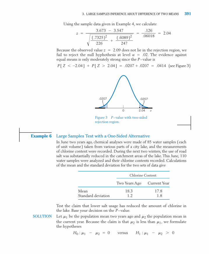
.0207 .0207
2.04 z0
Figure 3 P–value with two-sidedrejection region.
Using the sample data given in Example 4, we calculate
Because the observed value z � 2.09 does not lie in the rejection region, wefail to reject the null hyphothesis at level a � .02. The evidence againstequal means is only moderately strong since the P–value is
(see Figure 3)P [ Z �2.04 ] � P [ Z � 2.04 ] � .0207 � .0207 � .0414
z �3.673 � 3.547
� ( .7325 )2
226�
( .6089 )2
247
�.126
.06018� 2.04
3. LARGE SAMPLES INFERENCE ABOUT DIFFERENCE OF TWO MEANS 391
Chlorine Content
Two Years Ago Current Year
Mean 18.3 17.8Standard deviation 1.2 1.8
Example 6 Large Samples Test with a One-Sided AlternativeIn June two years ago, chemical analyses were made of 85 water samples (eachof unit volume) taken from various parts of a city lake, and the measurementsof chlorine content were recorded. During the next two winters, the use of roadsalt was substantially reduced in the catchment areas of the lake. This June, 110water samples were analyzed and their chlorine contents recorded. Calculationsof the mean and the standard deviation for the two sets of data give
Test the claim that lower salt usage has reduced the amount of chlorine inthe lake. Base your decision on the P–value.
SOLUTION Let be the population mean two years ago and the population mean in the current year. Because the claim is that is less than , we formulatethe hypotheses
� � � 0 versus � � � 0�2�1H1�2�1H0
�1�2
�2�1
c10a.qxd 10/15/09 11:13 AM Page 391

With the test statistic
the rejection region should be of the form R�Z � c because is right-sided.Using the data
we calculate
The significance probability of this observed value is ( see Figure 4)
P–value � P [ Z � 2.32 ] � .0102
Because the P–value is very small, we conclude that there is strong evidenceto reject and support .H1H0
z �18.3 � 17.8
� ( 1.2 )2
85�
( 1.8 )2
110
�.5
.2154� 2.32
s2 � 1.8y � 17.8n2 � 110s1 � 1.2x � 18.3n1 � 85
H1
Z �X � Y
� S21
n1�
S22
n2
392 CHAPTER 10/COMPARING TWO TREATMENTS
Testing : � � with Large Samples
Test statistic:
Alternative Hypothesis Level � Rejection Region
: � � R :Z �
: � R :Z � �
: � � R : � Z � � z�/2 0�2�1H1
z� 0�2�1H1
z� 0�2�1H1
Z �X � Y � 0
� S21
n1�
S22
n2
�0�2�1H0
.0102
2.32 z0
Figure 4 P–value � .0102.
We summarize the procedure for testing where is spec-ified under the null hypothesis. The case corresponds to � 0. 0�1 � �2
0�1 � �2 � 0
c10a.qxd 10/15/09 11:13 AM Page 392

3. LARGE SAMPLES INFERENCE ABOUT DIFFERENCE OF TWO MEANS 393
Finally, we would like to emphasize that with large samples we can alsolearn about other differences between the two populations.
Example 7 Large Samples Reveal Additional Differences between PopulationsNatural resource managers have attempted to use the Satellite Landsat Multi-spectral Scanner data for improved landcover classification. When the satellitewas flying over country known to consist of forest, the following intensitieswere recorded on the near-infrared band of a thermatic mapper. The samplehas already been ordered.
77 77 78 78 81 81 82 82 82 82 82 83 83 84 84 8484 85 86 86 86 86 86 87 87 87 87 87 87 87 89 8989 89 89 89 89 90 90 90 91 91 91 91 91 91 91 9191 91 93 93 93 93 93 93 94 94 94 94 94 94 94 9494 94 94 94 95 95 95 95 95 96 96 96 96 96 96 9797 97 97 97 97 97 97 97 98 99 100 100 100 100
100 100 100 100 100 101 101 101 101 101 101 102102 102 102 102 102 103 103 104 104 104 105 107
When the satellite was flying over urban areas, the intensities of reflectedlight on the same near-infrared band were
71 72 73 74 75 77 78 79 79 79 79 80 80 80 81 81 8182 82 82 82 84 84 84 84 84 84 85 85 85 85 85 85 8686 87 88 90 91 94
If the means are different, the readings could be used to tell urban fromforest area. Obtain a 95% confidence interval for the difference in mean radi-ance levels.
SOLUTION Computer calculations give
Forest Urban
Number 118 40Mean 92.932 82.075Standard deviation 6.9328 4.9789
and, for large sample sizes, the approximate 95% confidence interval for � is given by
Since � 1.96, the 95% confidence interval is calculated as
92.932 � 82.075 � 1.96 � ( 6.9328 )2
118�
( 4.9789 )2
40 or ( 8.87, 12.84 )
z.025
� X � Y � z.025 � S21
n1�
S22
n2, X � Y � z.025 � S2
1
n1�
S22
n2�
�2�1
c10a.qxd 10/15/09 11:13 AM Page 393

394 CHAPTER 10/COMPARING TWO TREATMENTS
The mean for the forest is 8.87 to 12.84 levels of radiance higher than themean for the urban areas.
Because the sample sizes are large, we can also learn about other differ-ences between the two populations. The stem-and-leaf displays and boxplotsin Figure 5 reveal that there is some difference in the standard deviation aswell as the means. The graphs further indicate a range of high readings thatare more likely to come from forests than urban areas. This feature hasproven helpful in discriminating between forest and urban areas on the basisof near-infrared readings.
778888899999
10101010
7812469034680247
781246903469024
24690346
024
24691346
025
25691346
02
3
791346
02
3
791
47
03
7
1
47
03
7
1
47
0
7
1
47
1
7
1
47
1
7
1
47
1
1
57
1
57
1
57
1
5 5
7777788888999
12478024680
4
35
90246
1
70
Forest Urban Forest Urban
80
90
100
110
90247
9124
91
4
1
4 5 5 5 5 5 5
Figure 5 Stem-and-leaf displays and boxplots give additional information aboutpopulation differences.
4. INFERENCES FROM SMALL SAMPLES: NORMAL POPULATIONS WITH EQUAL VARIANCES
Not surprisingly, more distributional structure is required to formulate appro-priate inference procedures for small samples. Here we introduce the smallsamples inference procedures that are valid under the following assumptionsabout the population distributions. Naturally, the usefulness of such proceduresdepends on how closely these assumptions are realized.
Additional Assumptions When the Sample Sizes Are Small
1. Both populations are normal.
2. The population standard deviations and are equal.�2�1
c10a.qxd 10/15/09 11:13 AM Page 394

A restriction to normal populations is not new. It was previously introduced forinferences about the mean of a single population. The second assumption,requiring equal variability of the populations, is somewhat artificial but wereserve comment until later. Letting s denote the common standard deviation,we summarize.
ESTIMATION
Again, is our choice for a statistic.
The common variance can be estimated by combining information providedby both samples. Specifically, the sum incorporates � 1pieces of information about , in view of the constraint that the deviations
sum to zero. Independently of this, contains � 1pieces of information about . These two quantities can then be combined,
to obtain a pooled estimate of the common . The proper divisor is the sumof the component degrees of freedom, or ( � 1) � ( � 1) � �
� 2.n2
n1n2n1
� 2
� ( Xi � X )2 � � ( Yi � Y )2
�2 n2�n2
i � 1 ( Yi � Y )2Xi � X
�2 n1�n1
i � 1 ( Xi � X )2�2
Var ( X � Y ) ��2
n1�
�2
n2� �2 �
1n1
�1n2
�Mean of ( X � Y ) � E ( X � Y ) � �1 � �2
X � Y
4. INFERENCES FROM SMALL SAMPLES: NORMAL POPULATIONS WITH EQUAL VARIANCES 395
Small Samples Assumptions
1. is a random sample from N ( , s).
2. is a random sample from N ( , s ).(Note: s is the same for both distributions.)
3. and are independent.Y1 , Y2 , . . . , Yn2X1 , X2 , . . . , Xn1
�2Y1 , Y2 , . . . , Yn2
�1X1 , X2 , . . . , Xn1
Pooled Estimator of the Common
�( n1 � 1 ) S2
1 � ( n2 � 1 ) S22
n1 � n2 � 2
S2pooled �
�n1
i � 1 ( Xi � X )2 � �
n2
i � 1 ( Yi � Y )2
n1 � n2 � 2
�2
c10a.qxd 10/15/09 11:13 AM Page 395

Example 8 Calculating the Pooled Estimate of VarianceCalculate the observed value from these two samples.
Sample from population 1: 8 5 7 6 9 7Sample from population 2: 2 6 4 7 6
SOLUTION The sample means are
Furthermore,
Thus, and the pooled variance is
The pooled variance is closer to 2 than 4 because the first sample size is larger.These arithmetic details serve to demonstrate the concept of pooling.
Using a calculator with a “standard deviation” key, one can directly getthe sample standard deviations � 1.414 and � 2.000. Noting that
� 6 and � 5, we can then calculate the pooled variance as
Employing the pooled estimator for the common s, we obtain aStudent’s t variable that is basic to inferences about �1 � �2 .
√S2pooled
s2pooled �
5 ( 1.414 )2 � 4 ( 2.000 )2
9� 2.89
n2n1
s2s1
s2pooled �
� ( xi � x )2 � �
( yi � y )2
n1 � n2 � 2�
10 � 166 � 5 � 2
� 2.89
s21 � 2, s2
2 � 4,
� ( 7 � 5 )2 � ( 6 � 5 )2 � 16
� ( 2 � 5 )2 � ( 6 � 5 )2 � ( 4 � 5 )2
( 5 � 1 ) s22 � �
( yi � y )2
� ( 9 � 7 )2 � ( 7 � 7 )2 � 10
� ( 8 � 7 )2 � ( 5 � 7 )2 � ( 7 � 7 )2 � ( 6 � 7 )2
(6 � 1)s21 � � ( xi � x )2
y �� yi
5�
255
� 5x �� xi
6�
426
� 7
s2pooled
396 CHAPTER 10/COMPARING TWO TREATMENTS
has Student’s t distribution with � � 2 degrees of freedom.n2n1
T �( X � Y ) � ( �1 � �2
)
Spooled � 1n1
�1n2
c10a.qxd 10/15/09 11:13 AM Page 396

We can now obtain confidence intervals for which are of theform
Example 9 Calculating a Small Samples Confidence IntervalBeginning male and female accounting students were given a test and, on thebasis of their answers, were assigned a computer anxiety score (CARS). Usingthe data given in Table D.4 of the Data Bank, obtain a 95% confidence inter-val for the difference in mean computer anxiety score between beginningmale and female accounting students.
SOLUTION The dot diagrams of these data, plotted in Figure 6, give the appearance ofapproximately equal amounts of variation.
Estimate of parameter � ( t value ) ( Estimated standard error )
�1 � �2,
4. INFERENCES FROM SMALL SAMPLES: NORMAL POPULATIONS WITH EQUAL VARIANCES 397
Confidence Interval for � Small Samples and �
A 100 (1 � a ) % confidence interval for is given by
where
and is the upper a /2 point of the t distribution with d.f. � � � 2.n2n1
t�/2
S2pooled �
( n1 � 1 ) S21 � ( n2 � 1 ) S2
2
n1 � n2 � 2
X � Y � t� / 2 Spooled � 1n1
�1n2
�1 � �2
�2��2�1
1 2Male CARS
3 4
1 2Female CARS
3 4
Figure 6 Dot diagrams of the computer anxiety data in Example 8.
We assume that the CARS data for both females and males are randomsamples from normal populations with means and , respectively, and�2�1
c10a.qxd 10/15/09 11:13 AM Page 397

a common standard deviation s. Computations from the data provide thesummary statistics:
Female CARS� 15 � .773
Male CARS� 20 � .525
We calculate
With a 95% confidence interval a / 2 � .025 and consulting the t table, wefind (interpolating) that � 2.035 for d.f. � � � 2 � 33.Thus a 95% confidence interval for � becomes
We can be 95% confident that the mean computer anxiety score for femalebeginning accounting students can be .003 to .895 units lower than the meanscore for males.
This interval is quite wide. Certainly the very small values representtechnically insignificant differences.
TESTS OF HYPOTHESES
Tests of hypotheses concerning the difference in means are based on a statistichaving student’s t distribution.
� � .449 � .446 or ( � .895, �.003 )
� 2.514 � 2.963 � 2.035 .642 � 115
�1
20
x � y � t0.25 spooled � 1n1
�1n2
�2�1
n2n1t.025
spooled � � 14 ( .773 )2 � 19 ( .525 )2
15 � 20 � 2� .642
s2y � 2.963n2
s1x � 2.514n1
398 CHAPTER 10/COMPARING TWO TREATMENTS
Testing H : � � � with Small Samples and �
Test statistic:
Alternative Hypothesis Level � Rejection Region
: � � R :T �
: � R :T � �
: � � R : � T � � t�/2 0�2�1H1
t� 0�2�1H1
t� 0�2�1H1
T �X � Y � 0
Spooled � 1n1
�1n2
d.f. � n1 � n2 � 2
�2�10�2�10
c10a.qxd 10/15/09 11:13 AM Page 398

Example 10 Testing the Equality of Mean Computer Anxiety ScoresRefer to the computer anxiety scores (CARS) described in Example 9 andthe summary statistics
Female CARS� 15 � .773
Male CARS� 20 � .525
Do these data strongly indicate that the mean score for females is lowerthan that for males? Test at level a � .05.
SOLUTION We are seeking strong evidence in support of the hypothesis that the meancomputer anxiety score for females ( ) is less than the mean score formales. Therefore the alternative hypothesis should be taken as : or : � 0, and our problem can be stated as testing
: � � 0 versus : � 0
We employ the test statistic
and set the left-sided rejection region R :T � �t.05. For d.f. � � �2 � 33, we approximate the tabled value as � 1.692, so the rejectionregion is R :T � �1.692.
With � .642 already calculated in Example 9, the observed valueof the test statistic T is
This value lies in the rejection region R. Consequently, at the .05 level of signif-icance, we reject the null hypothesis in favor of the alternative hypothesis thatmales have a higher mean computer anxiety score.
A computer calculation gives a P–value of about .025 so the evidence ofis moderately strong.
DECIDING WHETHER OR NOT TO POOL
Our preceding discussion of large and small sample inferences raises a few questions:
For small sample inference, why do we assume the population standarddeviations to be equal when no such assumption was needed in the largesamples case?
H1
t �2.514 � 2.963
.642 � 115
�1
20
��.449.2193
� �2.05
Spooled
t.05
n2n1
T �X � Y
Spooled � 1n1
�1n2
d.f. � n1 � n2 � 2
�2�1H1 �2�1H0
�2�1H1
�2�1H1
�1
s2y � 2.963n2
s1x � 2.514n1
4. INFERENCES FROM SMALL SAMPLES: NORMAL POPULATIONS WITH EQUAL VARIANCES 399
c10a.qxd 10/15/09 11:13 AM Page 399
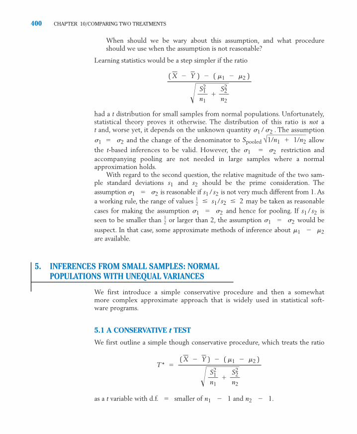
When should we be wary about this assumption, and what procedureshould we use when the assumption is not reasonable?
Learning statistics would be a step simpler if the ratio
had a t distribution for small samples from normal populations. Unfortunately,statistical theory proves it otherwise. The distribution of this ratio is not a t and, worse yet, it depends on the unknown quantity / . The assumption
� and the change of the denominator to allow
the t-based inferences to be valid. However, the � restriction andaccompanying pooling are not needed in large samples where a normalapproximation holds.
With regard to the second question, the relative magnitude of the two sam-ple standard deviations and should be the prime consideration. Theassumption � is reasonable if / is not very much different from 1. Asa working rule, the range of values may be taken as reasonablecases for making the assumption � and hence for pooling. If / isseen to be smaller than or larger than 2, the assumption � would be
suspect. In that case, some approximate methods of inference about �
are available.
5. INFERENCES FROM SMALL SAMPLES: NORMAL POPULATIONS WITH UNEQUAL VARIANCES
We first introduce a simple conservative procedure and then a somewhatmore complex approximate approach that is widely used in statistical soft-ware programs.
5.1 A CONSERVATIVE t TEST
We first outline a simple though conservative procedure, which treats the ratio
as a t variable with d.f. � smaller of � 1 and � 1.n2n1
T * �( X � Y ) � ( �1 � �2
)
� S21
n1�
S22
n2
�2�1
�2 �1 12
s2s1�2 �1
12 � s1
/ s2 � 2s2s1�2 �1
s2s1
�2 �1
Spooled √1/n1 � 1/n2�2 �1
�2 �1
( X � Y ) � ( �1 � �2 )
� S21
n1�
S22
n2
400 CHAPTER 10/COMPARING TWO TREATMENTS
c10a.qxd 10/15/09 11:13 AM Page 400

Here, the confidence interval is conservative in the sense that the actuallevel of confidence is at least 1 � a. Likewise, the level a test is conservativein the sense that the actual Type I error probability is no more than a.
Example 11 Testing Equality of Green Gas Mean YieldsOne process of making green gasoline, not just a gasoline additive, takes bio-mass in the form of sucrose and converts it into gasoline using catalytic reac-tions. This research is still at the pilot plant stage. At one step in a pilot plantprocess, the product volume ( liters) consists of carbon chains of length 3. Nineruns were made with each of two catalysts and the product volumes measured.
catalyst 1 1.86 2.05 2.06 1.88 1.75 1.64 1.86 1.75 2.13
catalyst 2 .32 1.32 .93 .84 .55 .84 .37 .52 .34
The sample sizes = = 9 and the summary statistics are
,
Is the mean yield with catalyst 1 more than .80 liters higher than the yieldwith catalyst 2? Test with a 5 0.05
SOLUTION The test concerns the d 5 � and we wish to show that d is greaterthan .80. Therefore we formulate the testing problem as
: � � .80 versus : � � .80
The sample sizes = = 9 are small and there are no outliers or obviousdepartures from normality. However, is more than four times
. We should not pool.We choose the conservative test which is based on the test statistic
s21 � .0269
s22 � .1133
n2n1
�2�1H1 �2�1H0
�2�1
s22 � .1133y � .670s2
1 � .0269x � 1.887
n2n1
5. INFERENCES FROM SMALL SAMPLES: NORMAL POPULATIONS WITH UNEQUAL VARIANCES 401
Small Samples Inferences for � When the PopulationsAre Normal But and Are Not Assumed to Be Equal
A 100 (1 � a)% conservative confidence interval for � is given by
where denotes the upper a/2 point of the t distribution with d.f. �smaller of � 1 and � 1.
The null hypothesis : � � is tested using the test statistic
T* �X � Y � 0
� S21
n1�
S22
n2
d.f. � smaller of n1 � 1 and n2 � 1
0�2�1H0
n2n1
t �/2
X � Y � t �/2 � S21
n1�
S22
n2
�2�1
�2�1
�2�1
c10a.qxd 10/15/09 11:13 AM Page 401

For d.f. � 8, the tabled value is � 1.860, so we set the rejection regionR : � 1.860. The calculated value of the test statistic is
which falls in the rejection region. So, we reject the null hypothesis at a = .05and conclude that the mean product volume from catalyst 1 is more than .80liters higher.
The associated P–value = Alternatively, the observed is only slightly smaller than the entry = 3.355 in Table 4,Appendix B.
The conservative procedure does guarantee that a is an upper bound on theprobability of falsely rejecting the null hypothesis. It is a reasonable choice whenthe minimum sample size, and therefore the degrees of freedom, are not too small.
5.2 AN APPROXIMATE t TEST—SATTERTHWAITE CORRECTION
An alternate, but more complicated approximation is available for two normaldistributions whose variances seem to be unequal. This approximate t distribu-tion is preferred over the conservative procedure which can have too few de-grees of freedom. The statistic is the same but, because sample sizes aresmall, its distribution is approximated as a t distribution. This approach issometimes called the Satterthwaite correction after the person who derived theapproximation.
T*
t.005t*
P [ T � 3.34 ] � .0051.
t* �1.887 � .670 � .80
� .02699
�.1133
9
� 3.34
T*
t.05
d.f. � smaller of n1 � 1 and n2 � 1� 8
T* �X � Y � 0
� S21
n1�
S22
n2
402 CHAPTER 10/COMPARING TWO TREATMENTS
Normal Populations with �
Let d = � . When the sample sizes and are not large and s1 s2
is approximately distributed as a t with estimated degrees of freedom.
T* �X � Y �
� S21
n1�
S22
n2
�n2n1�2�1
�2�1
The estimated degrees of freedom depend on the observed values of the sam-ple variances and .s2
2s21
c10a.qxd 10/15/09 11:13 AM Page 402

5. INFERENCES FROM SMALL SAMPLES: NORMAL POPULATIONS WITH UNEQUAL VARIANCES 403
estimated degrees of freedom =
The estimated degrees of freedom v are often rounded down to an integer so a ttable can be consulted.
Example 12 Confidence Interval Using the Approximate tRefer to Example 11. Use the approximate t distribution to determine a 95%confidence interval for the difference of mean product volumes.
SOLUTION From the previous example we have the summary statistics
, , ,
We first estimate the degrees of freedom
To use the t table, we round down to 11 and then obtain = 2.201 for11 degrees of freedom.
The resulting 95% confidence interval is
or ( .94, 1.49 ) liters. The mean product volume for the first catalyst is greaterthan that of the second catalyst by .94 to 1.49 liters.
Notice that the conservative procedure would use 8 d.f. so = 2.306and the resulting confidence interval is wider than ( .94, 1.49 ) liters.
When computer software is available to simplify the calculation, the ap-proximate t approach is usually preferred.
t.025
1.887 � .670 � 2.201� .026999
�.1133
9 �� 1.887 � .670 � 2.201� .02699
9�
.11339
,
t0.025
� 0.2699
�.1133
9 �2
19 � 1
� .02699 �2
�1
9 � 1 � .1133
9 �2 � 11.60
� S21
n1�
S22
n2�
2
1n1 � 1
� S21
n1�
2
�1
n2 � 1 � S2
2n2
�2 �
s22 � .1133y � .670s2
1 � .0269x � 1.887
v �� S2
1
n1�
S22
n2�
2
1n1 � 1
� S21
n1�2
�1
n2 � 1 � S2
2
n2�
2
c10a.qxd 10/15/09 11:13 AM Page 403

10.5 One semester, an instructor taught the samecomputer course at two universities located indifferent cities. He was able to give the samefinal at both locations. The student’s scoresprovided the summary statistics.
(a) Obtain a point estimate of �and calculate the estimated standard error.
(b) Construct a 95% confidence interval for � .
10.6 Rural and urban students are to be comparedon the basis of their scores on a nationwidemusical aptitude test. Two random samples ofsizes 90 and 100 are selected from rural andurban seventh-grade students. The summarystatistics from the test scores are
�2�1
�2�1
404 CHAPTER 10/COMPARING TWO TREATMENTS
10.9 Refer to Exercise 10.8. Perform a test of hy-pothesis that is intended to show that the meanfor magazine 1 is more than 2 words larger thanthe mean for magazine 2.
(a) Formulate the null and alternative hy-potheses. (Define any symbols you use.)
(b) State the test statistic and the rejectionregion with a � .05.
(c) Perform the test at a � .05. Also, findthe P–value and comment.
10.10 Refer to Example 4. Workers in three occupa-tions were questioned about satisfaction withtheir jobs. Suppose the number of responses ineach of the four categories are
Assign 1 to very dissatisfied, 2 to a little dissatis-fied, 3 to moderately satisfied, and 4 to very sat-isfied. These data have means and proportionvery satisfied similar to those reported in a largescale survey.
(a) Calculate the sample mean and varianceseparately for firefighters and office super-visors. The scores for clergy have mean3.79 and standard deviation .590.
(b) Construct a 95% confidence interval forthe difference in mean satisfaction scorefor clergy and office supervisors.
10.11 Refer to the confidence interval obtained inExercise 10.10 (b). If you were to test the nullhypothesis that the mean satisfaction scoresare equal versus the two-sided alternatives,what would be the conclusion of your testwith a � .05? (See Section 4 of Chapter 9.)
2
Sample 1 Sample 2
� 52 � 44
s22 � 142s2
1 � 151y � 66x � 73
n2n1
Exercises
Very A Little Moder- Very Dis- Dis- ately Satis- Sample
Occupation satisfied satisfied Satisfied fied Size
Firefighters 6 16 24 180 226
Office Supervisors 1 12 85 149 247
Clergy 1 5 6 78 90
General Social Survey 1988–2006 conducted by the NationalOpinion Research Center, University of Chicago.
2
Rural Urban
Sample size 90 100Mean 76.4 81.2Standard deviation 8.2 7.6
Construct a 98% confidence interval for thedifference in population mean scores betweenurban and rural students.
10.7 Perform a test to determine if there is a signifi-cant difference between the population meanscores in Exercise 10.6. Use a � .05.
10.8 A linguist wants to compare the writing styles intwo magazines and one measure is the number ofwords per sentence. On the basis of 50 randomlyselected sentences from each source, she finds
Determine a 98% confidence interval for the dif-ference in mean number of words per sentence.
Magazine 2 n2 � 50 y � 9.5 s2 � 1.9
Magazine 1 n1 � 50 x � 12.6 s1 � 4.2
c10a.qxd 10/15/09 11:13 AM Page 404

10.12 In a study of interspousal aggression and its possi-ble effect on child behavior, the behavior problemchecklist (BPC) scores were recorded for 47 chil-dren whose parents were classified as aggressive.The sample mean and standard deviation were7.92 and 3.45, respectively. For a sample of 38children whose parents were classified asnonaggressive, the mean and standard deviation ofthe BPC scores were 5.80 and 2.87, respectively.Do these observations substantiate the conjecturethat the children of aggressive families have ahigher mean BPC than those of nonaggressivefamilies? (Answer by calculating the P–value.)
10.13 Suppose that measurements of the size of but-terfly wings (cm) for two related speciesyielded the data
Species 1 6 4 7 3
Species 2 6 9 6
(a) Calculate
(b) Give an estimate of the common standarddeviation for the wing size for the twospecies.
(c) Evaluate the t statistic for testing equalityof the two population mean wing sizes.
10.14 Three male and three female students recordedthe number of times they used a credit card inone week.
Male 8 4 6
Female 1 5 3
(a) Calculate
(b) Give an estimate of the common standarddeviation for the number of uses.
(c) Evaluate that t statistic for testing equal-ity of the two population mean numberof uses.
10.15 Two gel pens, Gel-1 and Gel-2, are compared onthe basis of the number of weeks before theystop writing. Out of 27 persons available, 13 arerandomly chosen to receive Gel-1 and the other14 receive Gel-2. These are the only pens theyuse for writing.
s2pooled .
s2pooled .
5. INFERENCES FROM SMALL SAMPLES: NORMAL POPULATIONS WITH UNEQUAL VARIANCES 405
Abused Nonabused
Mean 2.48 1.57Standard deviation 1.94 1.31
� 13, �
� 14, �
(a) Obtain
(b) Test � � against � �
with a � .05.
(c) Determine a 95% confidence interval for� .
10.16 The data on the weight (lb) of male and femalewolves, from Table D.9 of the Data Bank, are
Female 57 84 90 71 71 77 68 73
Male 71 93 101 84 88 117 86 86 93 86 106
(a) Test the null hypothesis that the meanweights of males and females are equal ver-sus a two-sided alternative. Take a � .05.
(b) Obtain a 95% confidence interval for thedifference of population mean weights.
(c) State any assumptions you make aboutthe populations.
10.17 Psychologists have made extensive studies onthe relationship between child abuse and latercriminal behavior. Consider a study that con-sisted of the follow-ups of 52 boys who wereabused in their preschool years and 67 boyswho were not abused. The data of the numberof criminal offenses of those boys in their teensyielded the following summary statistics.
Is the mean number of criminal offenses signif-icantly higher for the abused group than thatfor the nonabused group? Answer by calculat-ing the P–value.
10.18 Referring to the data in Exercise 10.17, deter-mine a 99% confidence interval for the differ-ence between the true means for the two groups.
10.19 To compare two programs for training indus-trial workers to perform a skilled job, 20workers are included in an experiment. Ofthese, 10 are selected at random and trained
�2�1
�2
�1H1 �2�1H0
s2pooled .
� 32( yi � y )2y � 17, n2
� 28( xi � x )2x � 9,n1
c10a.qxd 10/15/09 11:13 AM Page 405

406 CHAPTER 10/COMPARING TWO TREATMENTS
by method 1; the remaining 10 workers aretrained by method 2. After completion oftraining, all the workers are subjected to atime-and-motion test that records the speedof performance of a skilled job. The followingdata are obtained.
(a) Can you conclude from the data thatthe mean job time is significantly less aftertraining with method 1 than after trainingwith method 2? (Test with a � .05.)
(b) State the assumptions you make for thepopulation distributions.
(c) Construct a 95% confidence interval forthe population mean difference in jobtimes between the two methods.
10.20 Given here are the sample sizes and the samplestandard deviations for independent randomsamples from two populations. For each case,state which of the three tests you would use intesting hypotheses about � : (1) Z test,(2) t test with pooling, (3) conservative t testwithout pooling. Also, state any assumptions youwould make about the population distributions.(a)
(b)
(c)
(d)
10.21 Two different sprays for rewaterproofing parkasare compared by treating 5 parkas with spray 1and 6 with spray 2. After one day, each parka issprayed with water and the parka is rated on itsability to repel water. The following conclusionis reported
“Under the assumption of normal popula-tions with equal but unknown standard
n2 � 60, s2 � 2.1
n1 � 70, s1 � 6.2
n2 � 15, s2 � 5.36n1 � 8, s1 � 1.54
n2 � 7, s2 � 1.12
n1 � 8, s1 � 0.86
n2 � 50, s2 � 8.6
n1 � 35, s1 � 12.2
�2�1
deviations, the 90% confidence interval for � is ( 3.6, 5.2).”
From this report,
State the conclusion of testing : �
� 4.1 versus : � � 4.1 at a � .10. (See Section 4 of Chapter 9.)
10.22 To compare the effectiveness of isometric and iso-tonic exercise methods, 20 obese male studentsare included in an experiment: 10 are selected atrandom and assigned to one exercise method; theremaining 10 are assigned to the other exercisemethod. After five weeks, the reductions in ab-domen measurements are recorded in centimeters,and the following results are obtained.
(a) Do these data support the claim that theisotonic method is more effective?
(b) Construct a 95% confidence interval for� .
10.23 Refer to Exercise 10.22.
(a) Aside from the type of exercise method,identify a few other factors that are likelyto have an important effect on theamount of reduction accomplished in afive-week period.
(b) What role does randomization play inachieving a valid comparison between thetwo exercise methods?
(c) If you were to design this experiment,describe how you would divide the 20students into two groups.
10.24 Refer to Example 11.
(a) Using the conservative approach in Exam-ple 11, obtain an approximate 95% confi-dence interval for the difference of means.
(b) Compare the confidence interval in Part (a)with the one obtained in Example 12.
10.25 Refer to Exercise 10.24. Using the approximatet distribution as in Example 12, perform thetest requested in Example 11.
�A�B
�2�1H1 �2
�1H0
�2�1
Time (minutes)
Method 1 15 20 11 23 16 21 18 16 27 24
Method 2 23 31 13 19 23 17 28 26 25 28
Isometric IsotonicMethod A Method B
Mean 2.4 3.2Standard deviation 0.8 1.0
c10a.qxd 10/15/09 11:13 AM Page 406

10.26 The following generic computer output sum-marizes the data, given in Table D.5 of theData Bank, on the pretest percent body fat inmale and female students.
Gender N Mean StDevM 40 14.38 7.34F 43 23.72 5.78
Find a 99% confidence interval for the differ-ence of the two population means.
10.27 Refer to the data on the weight of wolves inTable D.9 of the Data Bank. A computeranalysis produces the output
6. RANDOMIZATION AND ITS ROLE IN INFERENCE 407
Two-sample T for Male wt vs Female wt
N Mean StDevMale wt 11 91.9 12.4Female wt 8 73.9 10.1T-Test of difference = 0 (vs not =):T-Value = 3.38 P-Value = 0.004 DF = 17
(a) What is the conclusion to testing the equal-ity of mean weights at level a � .05?
(b) Test the null hypothesis that males weighan average of 5 pounds more thanfemales against a two-sided alternative.Take a � .05.
6. RANDOMIZATION AND ITS ROLE IN INFERENCE
We have presented the methods of drawing inferences about the differencebetween two population means. Let us now turn to some important questionsregarding the design of the experiment or data collection procedure. The man-ner in which experimental subjects are chosen for the two treatment groups canbe crucial. For example, suppose that a remedial-reading instructor has devel-oped a new teaching technique and is permitted to use the new method toinstruct half the pupils in the class. The instructor might choose the most alertor the students who are more promising in some other way, leaving the weakerstudents to be taught in the conventional manner. Clearly, a comparisonbetween the reading achievements of these two groups would not just be acomparison of two teaching methods. A similar fallacy can result in comparingthe nutritional quality of a new lunch package if the new diet is given to agroup of children suffering from malnutrition and the conventional diet is givento a group of children who are already in good health.
When the assignment of treatments to experimental units is under our con-trol, steps can be taken to ensure a valid comparison between the two treat-ments. At the core lies the principle of impartial selection, or randomization.The choice of the experimental units for one treatment or the other must bemade by a chance mechanism that does not favor one particular selection overany other. It must not be left to the discretion of the experimenters because,even unconsciously, they may be partial to one treatment.
Suppose that a comparative experiment is to be run with N experimentalunits, of which units are to be assigned to treatment 1 and the remaining
� N � units are to be assigned to treatment 2. The principle of ran-domization tells us that the units for treatment 1 must be chosen at random
from the available collection of N units—that is, in a manner such that all
possible choices are equally likely to be selected.�N
n1�
n1
n1n2
n1
c10a.qxd 10/15/09 11:13 AM Page 407

Of course, in many cases, the investigator does not have the luxury of ran-domization. Consider comparing crime rates of cities before and after a newlaw. Aside from a package of criminal laws, other factors such as poverty, infla-tion, and unemployment play a significant role in the prevalence of crime. Aslong as these contingent factors cannot be regulated during the observationperiod, caution should be exercised in crediting the new law if a decline in thecrime rate is observed or discrediting the new law if an increase in the crimerate is observed. When randomization cannot be performed, extreme cautionmust be exercised in crediting an apparent difference in means to a difference intreatments. The differences may well be due to another factor.
As a practical method of random selection, we can label the available unitsfrom 1 to N. Then read random digits from Table 1, Appendix B, until differ-ent numbers between 1 and N are obtained. These experimental units receivetreatment 1 and the remaining units receive treatment 2. For a quicker andmore efficient means of random sampling, one can use the computer (see, forinstance, the Technology section, page 164, Chapter 4).
Although randomization is not a difficult concept, it is one of the most funda-mental principles of a good experimental design. It guarantees that uncontrolledsources of variation have the same chance of favoring the response of treatment 1as they do of favoring the response of treatment 2. Any systematic effects of un-controlled variables, such as age, strength, resistance, or intelligence, are choppedup or confused in their attempt to influence the treatment responses.
n1
n1
408 CHAPTER 10/COMPARING TWO TREATMENTS
Exercises
Randomization Procedure for Comparing Two Treatments
From the available N � � experimental units, choose units atrandom to receive treatment 1 and assign the remaining units to treat-
ment 2. The random choice entails that all possible selections are
equally likely to be chosen.
�Nn1�
n2
n1n2n1
Randomization prevents uncontrolled sources of variation from influenc-ing the responses in a systematic manner.
10.28 Randomly allocate 2 subjects from among
Al, Bob, Carol, Ellen, John
to be in the control group. The others willreceive a treatment.
10.29 Randomly allocate three subjects from among6 mice,
Alpha, Tau, Omega, Pi, Beta, Phi
to group 1.
c10a.qxd 10/15/09 11:13 AM Page 408

7. MATCHED PAIRS COMPARISONS 409
10.30 Early studies showed a disproportionate numberof heavy smokers among lung cancer patients.One scientist theorized that the presence ofa particular gene could tend to make a personwant to smoke and be susceptible to lung cancer.
(a) How would randomization settle thisquestion?
( b) Would such a randomization be ethicalwith human subjects?
10.31 Observations on 10 mothers who nursed theirbabies and 8 who did not revealed that nursingmothers felt warmer toward their babies. Canwe conclude that nursing affects a mother’sfeelings toward her child?
10.32 Suppose that you are asked to design an experi-ment to study the effect of a hormone injection
on the weight gain of pregnant rats during ges-tation. You have decided to inject 6 of the 12rats available for the experiment and retain theother 6 as controls.
(a) Briefly explain why it is important to ran-domly divide the rats into the two groups.What might be wrong with the experi-mental results if you choose to give thehormone treatment to 6 rats that are easyto grab from their cages?
(b) Suppose that the 12 rats are tagged with se-rial numbers from 1 through 12 and 12marbles identical in appearance are alsonumbered from 1 through 12. How can youuse these marbles to randomly select therats in the treatment and control groups?
7. MATCHED PAIRS COMPARISONS
In comparing two treatments, it is desirable that the experimental units or sub-jects be as alike as possible, so that a difference in responses between the twogroups can be attributed to differences in treatments. If some identifiable condi-tions vary over the units in an uncontrolled manner, they could introduce a largevariability in the measurements. In turn, this could obscure a real difference intreatment effects. On the other hand, the requirement that all subjects be alikemay impose a severe limitation on the number of subjects available for a compar-ative experiment. To compare two analgesics, for example, it would be impracticalto look for a sizable number of patients who are of the same sex, age, and generalhealth condition and who have the same severity of pain. Aside from the questionof practicality, we would rarely want to confine a comparison to such a narrowgroup. A broader scope of inference can be attained by applying the treatments ona variety of patients of both sexes and different age groups and health conditions.
Matched Pairs DesignMatched pair Experimental units
1
2
2
3
n
1
2 1
1 2
1 2
Units in each pair are alike, whereas units in different pairs may be dissim-ilar. In each pair, a unit is chosen at random to receive treatment 1, theother unit receives treatment 2.
c10a.qxd 10/15/09 11:13 AM Page 409

The concept of matching or blocking is fundamental to providing a com-promise between the two conflicting requirements that the experimental unitsbe alike and also of different kinds. The procedure consists of choosing units inpairs or blocks so that the units in each block are similar and those in differentblocks are dissimilar. One of the units in each block is assigned to treatment 1,the other to treatment 2. This process preserves the effectiveness of a compari-son within each block and permits a diversity of conditions to exist in differentblocks. Of course, the treatments must be allotted to each pair randomly to
410 CHAPTER 10/COMPARING TWO TREATMENTS
Matched Pairs
Identical twins are the epitome of matched pair experimental subjects.They are matched with respect to not only age but also a multitude ofgenetic factors. Social scientists, trying to determine the influence ofenvironment and heredity, have been especially interested in studyingidentical twins who were raised apart. Observed differences in IQ andbehavior are then supposedly due to environmental factors.
When the subjects are animals like mice, two from the same litter canbe paired. Going one step further, genetic engineers can now provide twoidentical plants or small animals by cloning these subjects.
iStockphoto
c10a.qxd 10/15/09 11:13 AM Page 410

avoid selection bias. This design is called a matched pairs design or sampling.For example, in studying how two different environments influence the learningcapacities of preschoolers, it is desirable to remove the effect of heredity: Ideally,this is accomplished by working with twins.
In a matched pairs design, the response of an experimental unit is influ-enced by:
1. The conditions prevailing in the block (pair).
2. A treatment effect.
By taking the difference between the two observations in a block, we can filterout the common block effect. These differences then permit us to focus on theeffects of treatments that are freed from undesirable sources of variation.
7. MATCHED PAIRS COMPARISONS 411
Pairing (or Blocking )
Pairing similar experimental units according to some identifiable charac-teristic(s) serves to remove this source of variation from the experiment.
The structure of the observations in a paired comparison is given below,where X and Y denote the responses to treatments 1 and 2, respectively. Thedifference between the responses in each pair is recorded in the last column,and the summary statistics are also presented.
Structure of Data for a Matched Pair Comparison
Pair Treatment 1 Treatment 2 Difference
1 � �2 � �. . . .. . . .. . . .n � �
The differences , , . . . , are a random sample.Summary statistics:
D �1n
�n
i � 1 Di S2
D �
�n
i � 1 (Di � D )2
n � 1
DnD2D1
YnXnDnYnXn
Y2X2D2Y2X2
Y1X1D1Y1X1
c10a.qxd 10/15/09 11:13 AM Page 411

412 CHAPTER 10/COMPARING TWO TREATMENTS
Although the pairs ( , ) are independent of one another, and within the ith pair will usually be dependent. In fact, if the pairing of experi-mental units is effective, we would expect and to be relatively largeor small together. Expressed in another way, we would expect ( , ) to have ahigh positive correlation. Because the differences � � , i � 1, 2,. . . , n, are freed from the block effects, it is reasonable to assume that theyconstitute a random sample from a population with mean and variancewhere represents the mean difference of the treatment effects. In other words,
If the mean difference is zero, then the two treatments can be consideredequivalent. A positive signifies that treatment 1 has a higher mean responsethan treatment 2. Considering , . . . , to be a single random sample froma population, we can immediately apply the techniques discussed in Chapters 8and 9 to learn about the population mean .
7.1 INFERENCES FROM A LARGE NUMBER OF MATCHED PAIRS
As we learned in Chapter 8, the assumption of an underlying normal distribu-tion can be relaxed when the sample size is large. The central limit theoremapplied to the differences , . . . , suggests that when n is large, say,greater than 30,
Inferences can then be based on the percentage points of the N (0, 1) distribu-tion or, equivalently, those of the t distribution, with the degrees of freedommarked “infinity.”
Example 13 Does Conditioning Reduce Percent Body Fat?A conditioning class is designed to introduce students to a variety of trainingtechniques to improve fitness and flexibility. The percent body fat was mea-sured at the start of the class and at the end of the semester. The data for81 students are given in Table D.5 of the Data Bank.
(a) Obtain a 98% confidence interval for the mean reduction in percentbody fat.
(b) Test, at a � .01, to establish the claim that the conditioning classreduces the mean percent body fat.
SOLUTION (a) Each subject represents a block which produces one measurement ofpercent body fat at the start of the semester (x) and one at the end (y).The 81 paired differences � � are summarized using acomputer.
yixidi
D � �D
SD / √n is approximately N ( 0, 1 )
DnD1
�D
DnD1
�D
�D
Var ( Di ) � �2
D i � 1, . . . , n E ( Di
) � �D
�D
�2D ,�D
YiXiDi
YiXi
YiXi
YiXiYiXi
c10a.qxd 10/15/09 11:13 AM Page 412

N Mean StDev SE MeanDifference 81 3.322 2.728 0.303
That is, � 3.322 and � 2.728. The sample size 81 is large sothere is no need to assume that the population is normal. Since, fromthe normal table, � 2.33, the 98% confidence interval becomes
or ( 2.62, 4.03) percent. We are 98% confident that the mean reductionin body fat is 2.62 to 4.03 percent.
(b) Because the claim is that � 0, the initial reading tends to behigher than at the end of class, we formulate:
The test statistic
is approximately normally distributed so the rejection region is R � Z �� 2.33. The observed value of the test statistic
falls in the rejection region. Consequently is rejected in favor ofat level a = .01. We conclude that the conditioning class does
reduce the mean percent body fat. The value of the test statistic isso far in the rejection region that the P–value is .0000 to at leastfour places. The evidence in support of is very very strong.
7.2 INFERENCES FROM A SMALL NUMBER OF MATCHED PAIRS
When the sample size is not large, we make the additional assumption that thedistribution of the differences is normal.
H1
H1
H0
z �d–
SD � √81�
3.322
2.728 � √81�
3.322.303
� 10.96
z.01
Z �D––
SD �√n
H0 : mD � 0 versus H1 : mD � 0
mD
( 3.322 � .706, 3.322 � .706 )
� 3.322 � 2.33 2.728
√81 , 3.322 � 2.33
2.728
√81 � �
� d–
� 2.33 sD
√81 , d
–� 2.33
sD
√81 �
z.01
sDd
7. MATCHED PAIRS COMPARISONS 413
c10a.qxd 10/15/09 11:13 AM Page 413

In summary,
414 CHAPTER 10/COMPARING TWO TREATMENTS
Small Samples Inferences about the Mean Difference
Assume that the differences � � are a random sample from anN ( , ) distribution. Let
and
Then:
1. A 100 (1 � a )% confidence interval for is given by
where is based on n � 1 degrees of freedom.
2. A test of : � is based on the test statistic
T �D � �D 0
SD / √n d.f. � n � 1
mD 0mDH0
t� /2
� D � t�/2 SD
√n, D � t�/2
SD
√n �
mD
SD � � �n
i � 1 (Di � D )2
n � 1D �
�n
i � 1 Di
n
�D mD
YiXiDi
�D
Example 14 Does a Pill Incidentally Reduce Blood Pressure?A medical researcher wishes to determine if a pill has the undesirable sideeffect of reducing the blood pressure of the user. The study involves record-ing the initial blood pressures of 15 college-age women. After they use thepill regularly for six months, their blood pressures are again recorded. Theresearcher wishes to draw inferences about the effect of the pill on bloodpressure from the observations given in Table 1.
(a) Calculate a 95% confidence interval for the mean reduction inblood pressure.
( b) Do the data substantiate the claim that use of the pill reduces bloodpressure? Test at a � .01.
TABLE 1 Blood-Pressure Measurements before and after Use of Pill
Subject
1 2 3 4 5 6 7 8 9 10 11 12 13 14 15
Before (x) 70 80 72 76 76 76 72 78 82 64 74 92 74 68 84After ( y) 68 72 62 70 58 66 68 52 64 72 74 60 74 72 74
d � x � y 2 8 10 6 18 10 4 26 18 � 8 0 32 0 � 4 10
Courtesy of a family planning clinic.
c10a.qxd 10/15/09 11:13 AM Page 414

7. MATCHED PAIRS COMPARISONS 415
SOLUTION (a) Here each subject represents a block generating a pair of measurements:one before using the pill and the other after using the pill. The paireddifferences � � are computed in the last row of Table 1, andwe calculate the summary statistics
If we assume that the paired differences constitute a random samplefrom a normal population N ( , ), a 95% confidence interval forthe mean difference is given by
where is based on d.f. � 14. From the t table, we find �2.145. The 95% confidence interval is then computed as
This means that we are 95% confident the mean reduction of bloodpressure is between 2.72 and 14.88.
( b) Because the claim is that � 0, we formulate
: � 0 versus : � 0
We employ the test statistic and set a right-sided
rejection region. With d.f. � 14, we find � 2.624, so the rejectionregion is R :T � 2.624.
The observed value of the test statistic
falls in the rejection region. Consequently, is rejected in favor of at a � .01. We conclude that a reduction in blood pressure followinguse of the pill is strongly supported by the data.
Note: To be more convinced that the pill causes the reduction inblood pressure, it is advisable to measure the blood pressures of thesame subjects once again after they have stopped using the pill for aperiod of time. This amounts to performing the experiment in reverseorder to check the findings of the first stage.
H1 H0
t �d
SD / √n�
8.80
10.98 / √15�
8.802.84
� 3.10
t.01
T �D
SD / √n , d.f. � 14
mDH1 mDH0
mD
8.80 � 2.145 10.98
√15� 8.80 � 6.08 or ( 2.72, 14.88 )
t.025t.025
D � t.025 SD
√15
mD
�D mD
d �� di
15� 8.80 sD � �� ( di � d )2
14� 10.98
yixidi
c10a.qxd 10/15/09 11:13 AM Page 415

416 CHAPTER 10/COMPARING TWO TREATMENTS
7.3 RANDOMIZATION WITH MATCHED PAIRS
Example 14 is a typical before–after situation. Data gathered to determine theeffectiveness of a safety program or an exercise program would have the samestructure. In such cases, there is really no way to choose how to order the experi-ments within a pair. The before situation must precede the after situation. Ifsomething other than the institution of the program causes performance toimprove, the improvement will be incorrectly credited to the program. However,when the order of the application of treatments can be determined by the inves-tigator, something can be done about such systematic influences. Suppose that acoin is flipped to select the treatment for the first unit in each pair. Then theother treatment is applied to the second unit. Because the coin is flipped againfor each new pair, any uncontrolled variable has an equal chance of helping theperformance of either treatment 1 or treatment 2. After eliminating an identifiedsource of variation by pairing, we return to randomization in an attempt toreduce the systematic effects of any uncontrolled sources of variation.
Randomization with Pairing
After pairing, the assignment of treatments should be randomized for each pair.
Randomization within each pair chops up or diffuses any systematic influencesthat we are unable to control.
Exercises
10.33 Given the following matched pairs sample,(a) Evaluate the t statistic
(b) How many degrees offreedom does this thave?
10.34 Two sun blockers are to be compared. Oneblocker is rubbed on one side of a subject’sback and the other blocker is rubbed on theother side. Each subject then lies in the sun fortwo hours. After waiting an additional hour,each side is rated according to redness.
(a) Evaluate the t statistic
(b) How many degrees of freedom does this thave?
t �d
SD / √n.
t �d
SD / √n.
10.35 It is claimed that an industrial safety program iseffective in reducing the loss of working hoursdue to factory accidents. The following data arecollected concerning the weekly loss of workinghours due to accidents in six plants both beforeand after the safety program is instituted.
Do the data substantiate the claim? Use a � .05.
Plant
1 2 3 4 5 6
Before 12 30 15 37 29 15After 10 29 16 35 26 16
x y
6 34 18 36 59 76 8
Subject No. Blocker 1 Blocker 2
1 2 22 7 53 8 44 3 15 5 3
c10a.qxd 10/15/09 11:13 AM Page 416

10.36 A manufacturer claims his boot waterproofingis better than the major brand. Five pairs ofshoes are available for a test.
(a) Explain how you would conduct a pairedsample test.
(b) Write down your assignment of water-proofing to each shoe. How did yourandomize?
10.37 A food scientist wants to study whether qual-ity differences exist between yogurt madefrom skim milk with and without the precul-ture of a particular type of bacteria, calledPsychrotrops (PC). Samples of skim milk areprocured from seven dairy farms. One-half ofthe milk sampled from each farm is inoculatedwith PC, and the other half is not. After yogurtis made with these milk samples, the firmnessof the curd is measured, and those measure-ments are given below.
(a) Do these data substantiate the conjec-ture that the treatment of PC results ina higher degree of curd firmness? Test ata � .05.
(b) Determine a 90% confidence interval forthe mean increase of curd firmness due tothe PC treatment.
10.38 A study is to be made of the relative effective-ness of two kinds of cough medicines inincreasing sleep. Six people with colds aregiven medicine A the first night and medicineB the second night. Their hours of sleep eachnight are recorded.
7. MATCHED PAIRS COMPARISONS 417
(a) Establish a 95% confidence interval forthe mean change in hours of sleep whenswitching from medicine A to medicine B.
( b) How and what would you randomize inthis study? Briefly explain your reason forrandomization.
10.39 Two methods of memorizing difficult materialare being tested to determine if one producesbetter retention. Nine pairs of students areincluded in the study. The students in eachpair are matched according to IQ and aca-demic background and then assigned to thetwo methods at random. A memorization testis given to all the students, and the followingscores are obtained:
At a � .05, test to determine if there is a sig-nificant difference in the effectiveness of thetwo methods.
10.40 In an experiment conducted to see if electricalpricing policies can affect consumer behavior,10 homeowners in Wisconsin had to pay a pre-mium for power use during the peak hours.They were offered lower off-peak rates. Foreach home, the July on-peak usage (kilowatthours) under the pricing experiment was com-pared to the previous July usage.
Dairy Farm
Curd Firmness A B C D E F G
With PC 68 75 62 86 52 46 72Without PC 61 69 64 76 52 38 68
Subject
1 2 3 4 5 6
Medicine A 4.8 4.1 5.8 4.9 5.1 7.4Medicine B 3.9 4.2 5.0 4.9 5.2 7.1
Pair
1 2 3 4 5 6 7 8 9
Method A 90 86 72 65 44 52 66 38 83Method B 85 87 70 62 44 53 62 35 86
Year
Previous Experimental
200 160180 175240 210425 370120 110333 298418 368380 250340 305516 477
c10a.qxd 10/15/09 11:13 AM Page 417

(a) Find a 95% confidence interval for themean decrease.
(b) Test � � 0 against � � 0at level a � .05.
(c) Comment on the feasibility of random-ization of treatments.
(d) Without randomization, in what waycould the results in parts (a) and ( b) bemisleading?
(Hint: What if air conditioner use is a primefactor, and the July with experimental pricingwas cooler than the previous July?)
10.41 To compare the crop yields from two strains ofwheat, A and B, an experiment was conductedat eight farms located in different parts of astate. At each farm, strain A was grown on oneplot and strain B on another; all 16 plots wereof equal sizes. Given below are data of yield inpounds per plot.
(a) Is there strong evidence that strain A hasa higher mean yield than strain B? Test at a � .05.
(b) What should be randomized in thisexperiment and how?
10.42 Refer to the problem stated in Exercise 10.41,but now suppose that the study was conductedat 16 farms, of which 8 were selected for
�DH1 �DH0
8. CHOOSING BETWEEN INDEPENDENT SAMPLES AND A MATCHED PAIRS SAMPLE
When planning an experiment to compare two treatments, we often have theoption of either designing two independent samples or designing a sample withpaired observations. Therefore, some comments about the pros and cons ofthese two sampling methods are in order here. Because a paired sample with npairs of observations contains 2n measurements, a comparable situation would
418 CHAPTER 10/COMPARING TWO TREATMENTS
Strain A 23 39 19 28 42 43 33 29Strain B 20 21 40 34 33 18 33 21
Farm
1 2 3 4 5 6 7 8
Strain A 23 39 19 43 33 29 28 42Strain B 18 33 21 34 33 20 21 40
planting strain A and the other 8 for strain B.Here also the plots used were all of equal sizes.Recorded below are the data of yields inpounds per plot.
(a) Is there strong evidence that strain A has ahigher mean yield than strain B? State theassumptions you make and use a � .05.
(b) What should be randomized in thisexperiment and how?
(c) Check to see that each data set here is just ascrambled form of the data set in Exercise10.41. Briefly explain why the conclusion ofyour test is different in the two situations.
10.43 Laser guns for detecting speeders require anaccurate measurement of distance. In one dailycalibration test, police measure the known dis-tances 164 feet and 104 feet. The difference inreadings should be 60 but there is some varia-tion. The differences for ten guns are (courtesyof Madison Police Department)
60.6 60.4 60.4 60.5 60.3 60.4 60.2 60.1 60.4 60.4
(a) Do the data provide strong evidence thatthe mean difference is not equal to 60 feet?
(b) Construct a 95% confidence interval forthe mean difference.
(c) Check that all of the values for mean dis-tance in the confidence interval, as well asall ten observations, are less than 1 percentof the exact 60 feet. Laser guns are muchmore accurate than the old radar guns.
c10a.qxd 10/15/09 11:13 AM Page 418

8. CHOOSING BETWEEN INDEPENDENT SAMPLES AND A MATCHED PAIR SAMPLE 419
be two independent samples with n observations in each. First, note that the samplemean difference is the same whether or not the samples are paired. This is because
Therefore, using either sampling design, the confidence intervals for the differ-ence between treatment effects have the common form
However, the estimated standard error as well as the degrees of freedom for tare different between the two situations.
Because the length of a confidence interval is determined by these two compo-nents, we now examine their behavior under the two competing sampling schemes.
Paired sampling results in a loss of degrees of freedom and, consequently,a larger value of . For instance, with a paired sample of n � 10, we have
� 1.833 with d.f. � 9. But the t value associated with independent sam-ples, each of size 10, is � 1.734 with d.f. � 18. Thus, if the estimatedstandard errors are equal, then a loss of degrees of freedom tends to make confi-dence intervals larger for paired samples. Likewise, in testing hypotheses, a lossof degrees of freedom for the t test results in a loss of power to detect realdifferences in the population means.
The merit of paired sampling emerges when we turn our attention to theother component. If experimental units are paired so that an interfering factor isheld nearly constant between members of each pair, the treatment responses X andY within each pair will be equally affected by this factor. If the prevailing conditionin a pair causes the X measurement to be large, it will also cause the correspondingY measurement to be large and vice versa. As a result, the variance of the differ-ence X � Y will be smaller in the case of an effective pairing than it will be in thecase of independent random variables. The estimated standard deviation will betypically smaller as well. With an effective pairing, the reduction in the standarddeviation usually more than compensates for the loss of degrees of freedom.
In Example 14, concerning the effect of a pill in reducing blood pressure, wenote that a number of important factors (age, weight, height, general health, etc.) af-fect a person’s blood pressure. By measuring the blood pressure of the same person
t.05
t.05
t�/2
( X � Y ) � t�/2 ( estimated standard error )
D �1n
� ( Xi � Yi
) � X � Y
Independent Samples Paired Sample( � � n ) ( n Pairs )
d.f. of t 2n � 2 n � 1
SD
√nSpooled � 1
n�
1n
Estimatedstandard error
n2n1
c10a.qxd 10/15/09 11:13 AM Page 419

before and after use of the pill, these influencing factors can be held nearly constantfor each pair of measurements. On the other hand, independent samples of onegroup of persons using the pill and a separate control group of persons not using thepill are apt to produce a greater variability in blood-pressure measurements if all thepersons selected are not similar in age, weight, height, and general health.
In summary, paired sampling is preferable to independent sampling when anappreciable reduction in variability can be anticipated by means of pairing. Whenthe experimental units are already alike or their dissimilarities cannot be linked toidentifiable factors, an arbitrary pairing may fail to achieve a reduction in variance.The loss of degrees of freedom will then make a paired comparison less precise.
9. COMPARING TWO POPULATION PROPORTIONS
We are often interested in comparing two populations with regard to the rate ofincidence of a particular characteristic. Comparing the jobless rates in two cities,the percentages of female employees in two categories of jobs, and infant mortal-ity in two ethnic groups are just a few examples. Let denote the proportion ofmembers possessing the characteristic in Population 1 and that in Population2. Our goals in this section are to construct confidence intervals for � andtest � � , the null hypothesis that the rates are the same for two popula-tions. The methods would also apply to the problems of comparison between twotreatments, where the response of a subject falls into one of two possible categoriesthat we may technically call “success” and “failure.” The success rates for the twotreatments can then be identified as the two population proportions and .
The form of the data is displayed in Table 2, where X and Y denote thenumbers of successes in independent random samples of sizes and takenfrom Population 1 and Population 2, respectively.
ESTIMATION
The population proportions of successes and are estimated by the corre-sponding sample proportions
p1 �Xn1
and p2 �Yn2
p2p1
n2n1
p2p1
p2p1H0
p2p1
p2
p1
420 CHAPTER 10/COMPARING TWO TREATMENTS
TABLE 2 Independent Samples from TwoDichotomous Populations
No. of No. of SampleSuccesses Failures Size
Population 1 X � XPopulation 2 Y � Y n2n2
n1n1
c10a.qxd 10/15/09 11:13 AM Page 420

Naturally, serves to estimate the difference � . Its standarderror is given by
where � 1 � and � 1 � . This formula of the standard errorstems from the fact that because and are based on independent samples,the variance of their difference equals the sum of their individual variances.
We can calculate the estimated standard error of by using theabove expression with the population proportions replaced by the correspond-ing sample proportions. Moreover, when and are large, the estimator
is approximately normally distributed. Specifically,
and this can be the basis for constructing confidence intervals for � .
Example 15 A Confidence Interval for a Difference in Success RatesAn investigation comparing a medicated patch with the unmedicated controlpatch for helping smokers quit the habit was discussed on page 88. At theend of the study, the number of persons in each group who were abstinentand who were smoking are repeated in Table 3.
Determine a 95% confidence interval for the difference in successprobabilities.
p2p1
Z �( p1 � p2 ) � ( p1 � p2
)
Estimated standard error is approximately N ( 0, 1 )
p1 � p2
n2n1
p1 � p2
p2p1
p2q2p1q1
S.E.( p1 � p2 ) � � p1q1
n1�
p2q2
n2
p2p1p1 � p2
9. COMPARING TWO POPULATION PROPORTIONS 421
TABLE 3 Quitting Smoking
Abstinent Smoking Total
Medicated patch 21 36 57Unmedicated patch 11 44 55
32 80 112
Large Samples Confidence Interval for p � p
An approximate 100 (1 � a ) % confidence interval for � is
provided the sample sizes and are large.n2n1
( p1 � p2 ) � z�/2 � p1 ( 1 � p1
)
n1�
p2 ( 1 � p2 )
n2
p2p1
21
c10a.qxd 10/15/09 11:13 AM Page 421

SOLUTION Let and denote the probabilities of quitting smoking with the med-icated and unmedicated patches, respectively. We calculate
A 95% confidence interval for � is
The confidence interval only covers positive values so we conclude that thesuccess rate with the medicated patch is .005 to .332 higher than for thecontrol group that received the untreated patches. The lower value is so closeto 0 that it is still plausible that the medicated patch is not very effective.
Note: A confidence interval for each of the population proportions and can be determined by using the method described in Section 5 ofChapter 8. For instance, with the data of Example 15, a 90% confidenceinterval for is calculated as
TESTING STATISTICAL HYPOTHESES
In order to formulate a test of � � when the sample sizes and arelarge, we again turn to the fact that is approximately normally distributed.But now we note that under the mean of this normal distribution is �
� 0 and the standard deviation is
where p stands for the common probability of success � and q � 1 � p.The unknown common p is estimated by pooling information from the twosamples. The proportion of successes in the combined sample provides
Also, Estimated S.E.( p1 � p2) � √ p q � 1n1
�1n2
or, alternatively, p �n1 p1 � n2 p2
n1 � n2
Pooled estimate p �X � Y
n1 � n2
p2p1
√p q � 1n1
�1n2
p2
p1H0
p1 � p2
n2n1p2p1H0
� .3684 � .1051 or ( .263, .474 )
p1 � 1.645 � p1 q1
n1� .3684 � 1.645 � .3684 .6316
57
p1
p2
p1
( .1684 � 1.96 .0836 , .1684 � 1.96 .0836 ) or ( .005, .332 )
p2p1
� p1 q1
n1�
p2 q2
n2� � .3684 .6316
57�
.2000 .800055
� .0836
p1 � p2 � .1684
p1 �2157
� .3684 p2 �1155
� .2000
p2p1
422 CHAPTER 10/COMPARING TWO TREATMENTS
c10a.qxd 10/15/09 11:13 AM Page 422

In summary,
Example 16 Testing Equality of Prevalence of a VirusA study (courtesy of R. Golubjatnikov) is undertaken to compare the rates of prevalence of CF antibody to parainfluenza I virus among boys and girls in the age group 5 to 9 years. Among 113 boys tested, 34 are found to have the antibody; among 139 girls tested, 54 have the antibody.Do the data provide strong evidence that the rate of prevalence of the antibodyis significantly higher in girls than boys? Use a � .05. Also, find the P–value.
SOLUTION Let denote the population proportion of boys who have the CF antibodyand the population proportion of girls who have the CF antibody. Becausewe are looking for strong evidence in support of , we formulate thehypotheses as
� � versus �
or equivalently as
� � � 0 versus � � 0
The sample sizes � 113 and � 139 being large, we will employ thetest statistic
and set a left-sided rejection region in view of the fact that is left-sided.With a � .05, the rejection region is R :Z � �1.645. We calculate
Pooled estimate p �34 � 54
113 � 139� .349
p1 �34
113� .301 p2 �
54139
� .388
H1
Z �p1 � p2
√ p q � 1n1
�1n2
n2n1
p2p1H0 p2p1H0
p2p1H1 p2p1H0
p2p1
p2
p1
9. COMPARING TWO POPULATION PROPORTIONS 423
Testing H �p � p with Large Samples
Test statistic:
The level a rejection region is accord-ing to whether the alternative hypothesis is � , p1 , or � .p2p1p2p2p1
� Z � � z�/2 , Z � �z� , or Z � z�
Z �p1 � p2
√ p ( 1 � p ) � 1n1
�1n2
where p �X � Y
n1 � n2
210
c10a.qxd 10/15/09 11:13 AM Page 423

424 CHAPTER 10/COMPARING TWO TREATMENTS
The observed value of the test statistic is then
Because the value z � � 1.44 is not in R, we do not reject . Conse-quently, the assertion that the girls have a higher rate of prevalence of the CF antibody than boys is not substantiated at the level of significancea � .05.
The significance probability of the observed z is
P–value � P [ Z � � 1.44]
� .0749
This means that we must allow an a of at least .0749 in order to consider theresult significant.
Exercises
H0
z �.301 � .388
√.349 .651 � 1113
�1
139
� �1.44
10.44 Refer to the measurement of job satisfaction inExample 4. Rather than average score, re-searchers often prefer the proportion who re-spond “very satisfied.” Using the data in Exercise10.10, compare the proportion for firefighters,
, with the proportion for office supervisors, .
(a) Find a 95% confidence interval for the dif-ference of proportions � .
(b) Perform the Z test for the null hypothe-sis � � versus � .Take a = .05
10.45 Refer to the measurement of job satisfaction inExercise 10.44. Using the data in Exercise10.10, compare the proportion for clergy, ,with the proportion for office supervisors, .
(a) Find a 95% confidence interval for the dif-ference of proportions � .
(b) Perform the Z test for the null hypothe-sis � � versus � � .Take a = .05
10.46 In a comparative study of two new drugs,A and B, 120 patients were treated with drugA and 150 patients with drug B, and the fol-lowing results were obtained.
p2p1H1p2p1H0
p2p1
p2
p1
p2p1H1p2p1H0
p2p1
p2p1
Attitude
Reactivity Submissive Resistant Total
HRL 34 15 49LRL 12 42 54
Drug A Drug B
Cured 50 88Not cured 70 62
Total 120 150
(a) Do these results demonstrate a signifi-cantly higher cure rate with drug B thandrug A? Test at a � .05.
(b) Construct a 95% confidence interval for thedifference in the cure rates of the two drugs.
10.47 In a study of the relationship between tempera-ment and personality, 49 female high school stu-dents who had a high level of reactivity (HRL)and 54 students who had a low level of reactivity(LRL) were classified according to their attitudeto group pressure with the following results.
c10a.qxd 10/15/09 11:13 AM Page 424

Is resistance to group pressure significantlylower in the HRL group than the LRL group?Answer by calculating the P–value.
10.48 Refer to the data in Exercise 10.47. Determinea 99% confidence interval for the differencebetween the proportions of resistant females inthe HRL and LRL populations.
10.49 Refer to Exercise 10.17 concerning a study onthe relationship between child abuse and latercriminal behavior. Suppose that from follow-ups of 85 boys who were abused in theirpreschool years and 120 boys who were notabused, it was found that 21 boys in the abusedgroup and 11 boys in the nonabused groupwere chronic offenders in their teens. Do thesedata substantiate the conjecture that abusedboys are more prone to be chronic offendersthan nonabused boys? Test at a � .01.
10.50 Referring to the data of Exercise 10.49, deter-mine a 95% confidence interval for the differ-ence between the true proportions of chronicoffenders in the populations of abused andnonabused boys.
10.51 The popular disinfectant Listerine is named afterJoseph Lister, a British physician who pioneeredthe use of antiseptics. Lister conjectured that hu-man infections might have an organic origin andthus could be prevented by using a disinfectant.Over a period of several years, he performed 75amputations: 40 using carbolic acid as a disinfec-tant and 35 without any disinfectant. The fol-lowing results were obtained.
9. COMPARING TWO POPULATION PROPORTIONS 425
Patient PatientSurvived Died Total
With carbolic acid 34 6 40Without carbolic acid 19 16 35
Hours of Sleep
Age � 8 � 8 Total
30–40 173 77 25060–70 120 130 250
Total 293 207 500
Are the survival rates significantly differentbetween the two groups? Test at a � .05 andcalculate the P–value.
10.52 Referring to the data of Exercise 10.51, calcu-late a 95% confidence interval for the differencebetween the survival rates for the two groups.
10.53 Random samples of 250 persons in the 30- to40-year age group and 250 persons in the 60-to 70-year age group are asked about the aver-age number of hours they sleep per night, andthe following summary data are recorded.
Do these data demonstrate that the proportionof persons who have � 8 hours of sleep pernight is significantly higher for the age group30 to 40 than that for the age group 60 to 70?Answer by calculating the P–value.
10.54 Referring to Exercise 10.53, denote by p1 and p2
the population proportions in the two groupswho have � 8 hours of sleep per night. Con-struct a 95% confidence interval for p1 � p2.
10.55 A medical researcher conjectures that smokingcan result in wrinkled skin around the eyes. Byobserving 150 smokers and 250 nonsmokers,the researcher finds that 95 of the smokers and103 of the nonsmokers have prominent wrin-kles around their eyes.(a) Do these data substantiate the belief that
prominent wrinkles around eyes aremore prevalent among smokers thannonsmokers? Answer by calculating theP–value.
(b) If the results are statistically significant,can the researcher readily conclude thatsmoking causes wrinkles around the eyes?Why or why not?
10.56 In the survey on which Table D.12 of the DataBank is based, a larger number of persons wasasked to respond to the statement “I would char-acterize my political beliefs as liberal” on a sevenpoint Likert scale from strongly disagree (1) tostrongly agree (7). A count of those whostrongly disagree, for each of three age groups,yielded the summary statistics.
c10a.qxd 10/15/09 11:13 AM Page 425

(a) Test equality of the proportions for the sec-ond two age groups versus a two-sided al-ternative. Take a � .05.
(b) Test equality of the proportions for the firsttwo age groups versus a two-sided alterna-tive. Take a � .05.
(c) Explain why the large samples test in Part (b)is not valid.
10.57 A major clinical trial of a new vaccine for type-Bhepatitis was conducted with a high-risk groupof 1083 male volunteers. From this group, 549men were given the vaccine and the other 534 aplacebo. A follow-up of all these individualsyielded the data:
426 CHAPTER 10/COMPARING TWO TREATMENTS
and also a group of drivers with no knownhealth conditions were retrieved from a motorvehicle department. Drivers in each groupwere classified according to their drivingrecord in the last year.
Let , , , and denote the populationproportions of drivers having one or more traf-fic violations in the last year for the fourgroups “diabetes,” “heart condition,” “epilepsy,”and “control,” respectively.
(a) Test � � versus � �at a � .10.
(b) Is there strong evidence that is higherthan ? Answer by calculating theP–value.
10.59 Refer to Exercise 10.58.
(a) Construct a 95% confidence interval for� .
(b) Construct a 90% confidence interval for� .
(c) Construct 95% confidence intervals for, , , and , individually.pCpEpHpD
pCpH
pHpE
pC
pE
pCpDH1pCpDH0
pCpEpHpD
Age xi ni pi
19–24 3 47 .063825–34 13 64 .203135–44 14 93 .1505
Follow-up
Did NotGot Hepatitis Get Hepatitis Total
Vaccine 11 538 549Placebo 70 464 534
(a) Do these observations testify that the vac-cine is effective? Use a � .01.
(b) Construct a 95% confidence interval for thedifference between the incidence rates ofhepatitis among the vaccinated and nonvac-cinated individuals in the high-risk group.
10.58 Records of drivers with a major medical condi-tion (diabetes, heart condition, or epilepsy)
Traffic Violations
Medical Condition None One or More Total
Diabetes 119 41 160Heart condition 121 39 160Epilepsy 72 78 150None (control) 157 43 200
USING STATISTICS WISELY
1. In all cases where a sample size is small and normality is assumed, the datashould be graphed in a dot plot to reveal any obvious outliers which couldinvalidate the inferences based on the normal theory.
2. When comparing two treatments under a matched pairs design, wheneverpossible, assign the treatments within each pair at random. To analyze theresulting data, use the results for one sample but applied to the differencesfrom each matched pair. For instance, if the difference of paired measurements
c10a.qxd 10/15/09 11:13 AM Page 426

KEY IDEAS AND FORMULAS 427
has a normal distribution, determine a 100 (1 � a)% confidence intervalfor the mean difference as
where is based on n � 1 degrees of freedom. Otherwise, with largesamples use .
3. When comparing two treatments using the independent samples design,randomly assign the treatments to groups whenever possible. With thematched pairs design, randomly assign the treatments within each pair.
4. When sample sizes are large, determine the limits of a 100 (1 � a)% con-fidence interval for the difference of means � as
5. When each of the two samples are from normal populations, having thesame variance, determine the limits of a 100 (1 � a)% confidence intervalfor the difference of means � as
where the pooled estimate of variance
and is based on � � 2 degrees of freedom.
6. Do not pool the two sample variances and if they are very dif-ferent. We suggest a factor of 4 as being too different. There are alternativeprocedures including the conservative procedure on page 400 and the ap-proximate t on page 402.
KEY IDEAS AND FORMULAS
In any comparative study of treatments, products, methods, and so on, the termtreatment refers to the things being compared. The basic unit or object, to whichone of the treatments is applied, is called an experimental unit or an experimentalsubject. The response variable is the characteristic that is recorded on each unit.
The specification of which treatment to compare and method of assigningexperimental units is called the experimental (or sampling) design. The choiceof appropriate statistical methods for making inferences depends heavily on theexperimental design chosen for data collection.
s22s2
1
n2n1t�/2
s2pooled �
( n1 � 1 ) s21 � ( n2 � 1 ) s2
2
( n1 � 1 ) � ( n2 � 1 )
x � y � t�/2 spooled � 1n1
�1n2
�2�1
x � y � z�/2 � s21
n1�
s22
n2
�2�1
z�/2
t�/2
� d � t�/2 SD
√n, d � t�/2
SD
√n �
mD
c10a.qxd 10/15/09 11:13 AM Page 427

A carefully designed experiment is fundamental to the success of a compar-ative study.
The most basic experimental designs to compare two treatments are inde-pendent samples and matched pairs sample.
The independent samples design require the subjects to be randomlyselected for assignment to each treatment. Randomization prevents uncon-trolled factors from systematically favoring one treatment over the other.
With a matched pairs design, subjects in each pair are alike, while those indifferent pairs may be dissimilar. For each pair, the two treatments should berandomly allocated to the members.
The idea of matching or blocking experimental units is to remove a knownsource of variation from comparisons. Pairing subjects according to some featureprevents that source of variation from interfering with treatment comparisons. Bycontrast, random allocation of subjects according to the independent random sam-pling design spreads these variations between the two treatments.
Inferences with Two Independent Random Samples
1. Large samples. When and are both greater than 30, inferences
about � are based on the fact that
A 100 (1 � a)% confidence interval for � is
To test � � � , we use the normal test statistic
No assumptions are needed in regard to the shape of the population distri-butions.
2. Small samples. When and are small, inferences using the t distri-bution require the assumptions:
(a) Both populations are normal.
(b) � .
The common s 2 is estimated by
S2pooled �
( n1 � 1)S21 � ( n2 � 1)S2
2
n1 � n2 � 2
�2 �1
n2n1
Z �( X � Y ) � 0
� S21
n1�
S22
n2
0 �2�1H0
X � Y � z�/2 � S21
n1�
S22
n2
�2�1
( X � Y ) � ( �1 � �2 )
� S21
n1�
S22
n2
is approximately N ( 0, 1 )
�2�1
n2n1
428 CHAPTER 10/COMPARING TWO TREATMENTS
c10a.qxd 10/15/09 11:13 AM Page 428

KEY IDEAS AND FORMULAS 429
Inferences about � are based on
A 100 (1 � a) % confidence interval for � is
To test : � � , the test statistic is
Inferences with a Matched Pair Sample
With a paired sample ( , ), . . . , ( , ), the first step is to calculate the differences � � , their mean and standard deviation S .
If n is small, we assume that the ’s are normally distributed N ( , ).Inferences about are based on
A 100 (1 � a)% confidence interval for is
The test of : � is performed with the test statistic:
If n is large, the assumption of normal distribution for the ’s is not needed.Inferences are based on the fact that
Summary of Inferences about Means
Table 4 summarizes all of the statistical procedures we have considered for mak-ing inferences about (1) a single mean, (2) the difference of two means, or (3) amean difference for a pair of observations.
Z �D � �D 0
SD � √n is approximately N ( 0, 1 )
Di
�D �D � �D 0
SD / √n d.f. � n � 1
�D�DH0
D � t� / 2 SD / √n
�D
T �D � �D
SD / √n d.f. � n � 1
�D
�D �DDi DD,Yi Xi Di
Yn Xn Y1 X1
T �( X � Y ) � 0
Spooled � 1n1
�1n2
d.f. � n1 � n2 � 2
0 �2�1H0
( X � Y ) � t�/2 Spooled � 1n1
�1n2
�2�1
T �( X � Y ) � ( �1 � �2
)
Spooled � 1n1
�1n2
d.f. � n1 � n2 � 2
�2�1
c10a.qxd 10/15/09 11:13 AM Page 429

TAB
LE 4
Gen
eral
For
mul
as fo
r In
fere
nces
ab
out
a M
ean
(m),
Diff
eren
ce o
f Tw
o M
eans
(m
� m
)
Ch.
8C
h.9
Ch.
10In
depe
nden
t Sa
mpl
esM
atch
ed S
ampl
es
Popu
lati
on(s
)G
ener
alN
orm
al w
ith
Nor
mal
Nor
mal
Gen
eral
Nor
mal
unkn
own
sN
(m,s
),N
(m,s
)N
(m,s
),N
(m,s
)fo
r th
e di
ffer
ence
s�
s�
ss
� s
D�
X
� Y
Infe
renc
e on
Mea
n m
Mea
n m
m�
mm
�
mm
�
mm
D�
m
� m
Sam
ple(
s)X
,.
..
,XX
,.
..
,X
X,
..
.,X
X,
..
.,X
X,
..
.,X
Y,
..
.,Y
Y.
..
,YY
,.
..
,Y
Sam
ple
size
nL
arge
n�
2
n�
2
n�
2
n�
30
n �
2
n�
30
n�
2
n�
2
n�
30
Poin
t es
tim
ator
Dis
trib
utio
nN
orm
altw
ith
twit
htw
ith
Nor
mal
twit
hd.
f.�
n
� 1
d.f.
� n
� n
� 2
d.f.
� sm
alle
r of
d.f.
� n
� 1
n�
1 an
d n
�1
Test
sta
tist
ic
D�
�D
0
S D/√
n
(X�
Y)
� 0
S poo
led �1 n 1
�1 n 2
21
21
3
S D √n�S2 1 n 1
�S2 2 n 2
�S2 1 n 1�
S2 2 n 2S p
oole
d �1 n 1
�1 n 2
S √nS √n
Est
imat
edst
d. d
ev.
�D √n
��2 1 n 1
��
2 2
n 2��
2 1 n 1�
�2 2
n 2�
�1 n 1�
1 n 2
� √n
� √n
�2 D n
�2 1
n 1�
�2 2
n 2
�2 1 n 1
��
2 2
n 2�
2 �1 n 1
�1 n 2�
�2 n
�2 n
D�
X�
YX
�Y
X�
YX
�Y
XX
22
2
11
1
2n
12
n1
2n
1
1n1
1n1
1n1
n1
n1
21
21
21
21
ii
i2
12
1
22
11
22
11
Tes
t st
atis
tic
�Po
int
esti
mat
or�
Para
met
er v
alue
at
H0
(nul
l hyp
othe
sis)
(Est
imat
ed o
r tr
ue)
std.
dev
. of
poin
t es
tim
ator
Con
fiden
ce in
terv
al�
Poin
t es
tim
ator
�(T
able
d va
lue)
(Est
imat
ed o
r tr
ue s
td. d
ev.)
21
(n1
�1)
S2 1�
(n2
�1)
S2 2
n 1�
n 2�
2
S2 pool
ed�
dev.
of t
he D
i’sS D
�sa
mpl
e st
d.
XY
D�
X
� Y
XY
D�
X
� Y
��
��
��
��
�X
YD
� X
� Y
nn
nn
n
22
22
21
11
11
(X�
Y)
� 0
�S2 1 n 1�
S2 2 n 2
(X�
Y)
� 0
�S2 1 n 1�
S2 2 n 2
X�
�0
S/√
n
X�
�0
S/√
n
Var
ianc
e of
poin
t es
tim
ator
Std.
dev.
ofpo
int
esti
mat
or
or e
stim
ated
by �s2 1 n 1
�s2 2 n 2�2
/ �( s12
� n 1
)2
( n1
�1)
�( s
22 �
n 2 )2
(n 2
�1
)�2
3
c10a.qxd 10/15/09 11:13 AM Page 430

Comparing Two Binomial Proportions—Large Samples
Data:
To test � � versus � � , use the Z test:
where
To test � � versus � � , use the Z test with R :Z � .A 100 (1 � a )% confidence interval for � is
TECHNOLOGY
Confidence intervals and tests for comparing means
MINITAB
Matched pair samples
We illustrate with the calculation of a 98% confidence interval and .02 level test.
Enter the first sample in C1 and second sample in C2.
Dialog box:
Stat � Basic Statistics � Paired t.Type C1 in First Sample and C2 in Second Sample.Click Options. Type 98 in Confidence level.Enter the value of the mean under the null hypothesis 0 in Test meanand choose not equal under the Alternative. Click OK. Click OK.
Two-sample t tests and confidence intervals
We illustrate with the calculation of a 98% confidence interval for � and.02 level test of the null hypothesis of no difference in means.
�2�1
( p1 � p2 ) � z� / 2 � p1 ( 1 � p1 )
n1�
p2 ( 1 � p2 )
n2
p2p1
z�p2p1H1 p2p1H0
p1 �Xn1
p2 �Yn2
p �X � Y
n1 � n2
Z �p1 � p2
√ p ( 1 � p ) � 1n1
�1n2
with R : � Z � � z�/2
p2p1H1 p2p1H0
Y � No. of successes in n2 trials with success probability P (S) � p2
X � No. of successes in n1 trials with success probability P (S) � p1
TECHNOLOGY 431
c10a.qxd 10/15/09 11:13 AM Page 431

Data:
C1 First sampleC2 Second sample
Dialog box:Stat � Basic Statistics � 2-Sample t.Select Samples in different columns. Type C1 in First and C2 in Second.To pool the estimates of variance, click the box Assume equal variances.Click Options. Type 98 in Confidence level, the null hypothesis valueof the mean 0 in Test mean, and select not equal under Alternative. ClickOK. Click OK.
EXCEL
Matched pairs t tests
We illustrate with the calculation of a test of the null hypothesis � � 0versus a two-sided alternative. Begin with values for the first variable in columnA and the second in column B.
Select Tools and then Data Analysis.Select t-Test: Paired Two-Sample for Means. Click OK.With the cursor in Variable 1 Range, highlight the data in column A.With the cursor in Variable 2 Range, highlight the data in column B.Type the hypothesized value 0 after Hypothesized mean difference.Click OK.
The program returns a summary that includes the value of the t statistic, theP–value for a one-sided test (actually the smallest tail probability), and theP–value for a two-sided test.
Two-sample t tests
We illustrate with a test of the null hypothesis of no difference betweenthe two means. Begin with the first sample in column A and the second incolumn B.
Select Tools and then Data Analysis.Select t-Test: Two-Sample Assuming Unequal Variances. Click OK or, topool, Select t-Test: Two-Sample Assuming Equal Variances and click OK.With the cursor in Variable 1 Range, highlight the data in column A.With the cursor in Variable 2 Range, highlight the data in column B.Type the hypothesized value 0 after Hypothesized mean difference.Enter .02 for Alpha. Click OK.
The program returns the one-sided and two-sided P–values.
�DH0
432 CHAPTER 10/COMPARING TWO TREATMENTS
c10b.qxd 10/15/09 11:14 AM Page 432

TI-84/-83 PLUS
Matched Pairs Samples
Confidence intervals
We illustrate the calculation of a 98% confidence interval. Start with the valuesfor the first variable entered in L1 and the second in L2.
Press STAT and select TESTS and then 8: Tinterval.Select Data with List set to L3 and Freq to 1.Enter .98 following C–Level: Select Calculate.Then press ENTER.
Tests
We illustrate the calculation of a test of the null hypothesis of 0 mean difference.Start with the first sample entered in L1 and the second in L2. Then let L3 �L2 � L1 or L3 � L1 � L2 depending on how the alternative is defined.
Press STAT and select TESTS and then 2: T-Test.Select Data with List set to L3 and Freq to 1.Enter 0 for . Select the direction of the alternative hypothesis for themean difference. Select Calculate.Press ENTER.
If, instead, the sample size, mean, and standard deviation are available, the sec-ond step is
Select Stats and type in the sample sizes, means, and standard deviations.
Two-sample t tests
We illustrate with the calculation of a test of the null hypothesis of no differ-ence between the two means. Start with the data entered in L1 and L2.
Press STAT and select TESTS and then 4: 2-SampT-Test.Select Data with List1 set to L1, List2 to L2, FREQ1 to 1, and Freq2to 1.Select the direction of the alternative hypothesis. Set Pooled to NO if youdo not wish to pool.Select Calculate or Draw and press ENTER.
The calculator will return the P–value. Draw will draw the t distribution andshade the area of the P–value. If, instead, the sample sizes, means, and standarddeviations are available, the second step is
Select Stats and enter the sample sizes, means, and standard deviations.
m0
TECHNOLOGY 433
c10b.qxd 10/15/09 11:14 AM Page 433

10. REVIEW EXERCISES
434 CHAPTER 10/COMPARING TWO TREATMENTS
10.60 Refer to Table D.12 of the Data Bank. The re-sponses, of persons in the first and second agegroups, on the frequency of credit card usequestion, have the summary statistics
(a) Obtain a 98% confidence interval for thedifference in the two population meanfrequency of credit card use scores.
(b) Test for equality of the two means versusa two-sided alternative. Use a � .02.
10.61 Two versions of a new simplified tax form, A1and A2, need to be evaluated with respect tothe time, in hours, it takes to complete theform. Forty persons were selected to fill outForm A1 and 40 were selected to fill out FormA2. The summary statistics are:
Form A1: � 12.2, � 1.1
Form A2: � 7.2, � 3.4
(a) Find a 95% confidence interval for the dif-ference in means.
(b) If only 80 persons are available for thisstudy, how would you choose the 40 touse form A1?
10.62 Refer to Table D.12 of the Data Bank. The re-sponses, of persons in the first and third agegroups to the average monthly amount charged,have the summary statistics
Determine a 95% confidence interval for thedifference of means.
10.63 Refer to the data in Exercise 10.62. Supposeyou wish to establish that the mean responseof 35–44 olds is larger than that of 19–24year olds by more than 150 dollars.
s2ys1x
(a) Formulate the null hypothesis and thealternative hypothesis.
(b) State the test statistic and the rejectionregion with a � .05.
(c) Perform the test at a � .05. Also, find theP–value and comment.
10.64 A study of postoperative pain relief is conductedto determine if drug A has a significantly longerduration of pain relief than drug B. Observationsof the hours of pain relief are recorded for 55patients given drug A and 58 patients given drugB. The summary statistics are
A B
Mean 4.64 4.03Standard deviation 1.25 1.82
(a) Formulate and .
(b) State the test statistic and the rejectionregion with a � .10.
(c) State the conclusion of your test with a �.10. Also, find the P–value and comment.
10.65 Consider the data of Exercise 10.64.
(a) Construct a 90% confidence interval for� .
(b) Give a 95% confidence interval for using the data of drug A alone. (Note:Refer to Chapter 8.)
10.66 Obtain for the gaming data in the chapteropening.
10.67 Given the following two samples,
8 11 5 9 7 and 5 3 4 8
obtain (a) and (b) the value of the t sta-tistic for testing : � � 2. State thed.f. of the t.
10.68 A fruit grower wishes to evaluate a new spraythat is claimed to reduce the loss due to damageby insects. To this end, he performs anexperiment with 27 trees in his orchard by treat-ing 12 of those trees with the new spray and the
m2m1H0
s2pooled
s2pooled
mA
mBmA
H1H0
Age
19–24 18 3.000 1.60925–34 28 4.429 1.643
sixini
Age
19–24 18 177.2 235.035–44 48 563.9 831.3
sixini
c10b.qxd 10/15/09 11:14 AM Page 434

10. REVIEW EXERCISES 435
other 15 trees with the standard spray. From thedata of fruit yield (in pounds) of those trees, thefollowing summary statistics were found.
(b) Construct a 98% confidence interval for thedifference in mean ages between A and B.
(c) Construct a 98% confidence interval forthe mean age for city A and city B indi-vidually. (Note: Refer to Chapter 8.)
10.72 The following generic computer output summa-rizes the data, given in Table D.6 of the DataBank, on the neck size of male and female bears.
Sex N Mean StDevF 36 52.92 8.83M 25 59.70 17.5
Test for equality of mean neck size versus atwo-sided alternative. Take � � .03.
10.73 Refer to the computer attitude scores (CAS) ofstudents given in Table D.4 of the Data Bank.A computer analysis produces the output
Two-sample T for CAS
sex N Mean StDevF 15 2.643 0.554M 20 2.945 0.390
Difference � mu M � mu FEstimate for difference: 0.30290\% CI for the difference(0.032, 0.571)T–Test of difference � 0(vs not �):T-Value � 1.89 P-Value � 0.067DF � 33Both use Pooled StDev � 0.467
(a) What is the conclusion to testing theequality of mean computer attitudescores at level � � .05?
(b) Find a 95% confidence interval for themean attitude score for males minus themean attitude score for females.
(c) Test the null hypothesis that, on average,males score .1 lower than females againsta two-sided alternative. Take � � .05.
10.74 In each of the following cases, how would youselect the experimental units and conduct theexperiment—matched pairs or independentsamples?
Do these data substantiate the claim that ahigher yield should result from the use of thenew spray? State the assumptions you makeand test at a � .05.
10.69 Referring to Exercise 10.68, construct a con-servative 95% confidence interval for the dif-ference in mean yields between the new sprayand the standard spray.
10.70 Refer to Exercise 10.61 but suppose, instead,that the sample sizes are 8 and 7 with the samesummary statistics:
Form A1: � 12.2, � 1.1
Form A2: � 7.2, � 3.4
(a) Test, with the conservative procedure,that the population means are different.Use a = .05.
(b) Test, with the approximate t procedure,that the population means are different.Use a = .05.
(c) What assumptions did you make for youranswer to Parts (a) and (b)?
10.71 An investigation is conducted to determine ifthe mean age of welfare recipients differsbetween two cities A and B. Random samplesof 75 and 100 welfare recipients are selectedfrom city A and city B, respectively, and thefollowing computations are made.
s2ys1x
New Spray Standard Spray
Mean yield 249 233Standard 19 45
deviation
City A City B
Mean 37.8 43.2Standard deviation 6.8 7.5
(a) Do the data provide strong evidence thatthe mean ages are different in city A andcity B? (Test at a � .02.)
c10b.qxd 10/15/09 11:14 AM Page 435

436 CHAPTER 10/COMPARING TWO TREATMENTS
(a) Compare the mileage obtained from twogasolines. Twelve SUVs of various sizesare available.
(b) Compare the drying times of two latex-based interior paints. Ten walls are available.
(c) Compare two methods of teaching swim-ming.Twenty five-year-old girls are available.
10.75 A sample of river water is divided into twospecimens. One is randomly selected to be sentto Lab A and the other is sent to Lab B. This isrepeated for a total of nine times. The measure-ment of suspended solids at Lab B is subtractedfrom that of Lab A to obtain the differences
12 10 15 42 11 �4 �2 10 �7
(a) Is there strong evidence that the mean dif-ference is not zero? Test with � � .02.
(b) Construct a 90% confidence interval forthe mean difference of the suspendedsolids measurements.
10.76 Two scales are available at a campus athletic facil-ity.A student wonders if, on average, they give thesame reading for weight. She and four othersweigh themselves on both scales.The readings are
other the standard fertilizer with the chemicaladditive. Plant growth after four weeks is mea-sured in centimeters. Do the following datasubstantiate the claim that use of the chemicaladditive accelerates plant growth? State the as-sumptions that you make and devise an appro-priate test of the hypothesis. Take � � .05.
Location
1 2 3 4 5 6 7 8 9 10
Without 20 31 17 22 19 32 25 18 21 19additive
With 23 34 16 21 22 31 29 20 25 23additive
Travel Time (minutes)
Path A 10 12 15 11 16 11Path B 12 15 17 13 18 16
10.78 Referring to Exercise 10.77, suppose that the twoplants at each location are situated in theeast–west direction. In designing this experiment,you must decide which of the two plants at eachlocation—the one in the east or the one in thewest—is to be given the chemical additive.
(a) Explain how, by repeatedly tossing a coin,you can randomly allocate the treatmentsto the plants at the 10 locations.
(b) Perform the randomization by actuallytossing a coin 10 times.
10.79 Students can bike to a park on the other side ofa lake by going around one side of the lake orthe other. After much discussion about whichwas faster, they decided to perform an experi-ment. Among the 12 students available, 6 wererandomly selected to follow Path A on one sideof the lake and the rest followed Path B on theother side. They all went on different days sothe conclusion would apply to a variety ofconditions.
Person Scale 1 Scale 2
1 113.8 114.12 218.7 217.23 149.2 147.34 104.9 103.55 166.6 165.7
(a) Find a 95% confidence interval for themean difference in scale readings.
(b) Based on your answer to Part (a), what is theconclusion to testing, with a = .05, that themean difference is 0 versus a two-sided alter-native hypothesis? Explain your reasoning.
(c) Explain how you would randomize in thisexperiment.
10.77 An experiment is conducted to determine if theuse of a special chemical additive with a stan-dard fertilizer accelerates plant growth. Ten lo-cations are included in the study. At each loca-tion, two plants growing in close proximity aretreated. One is given the standard fertilizer, the
(a) Is there a significant difference betweenthe mean travel times between the twopaths? State the assumptions you havemade in performing the test.
c10b.qxd 10/15/09 11:14 AM Page 436

10. REVIEW EXERCISES 437
(b) Suggest an alternative design for thisstudy that would make the comparisonmore effective.
10.80 Five pairs of tests are conducted to comparetwo methods of making rope. Each samplebatch contains enough hemp to make tworopes. The tensile strength measurements are
(a) Treat the data as 5 paired observations andcalculate a 95% confidence interval for themean difference in tensile strengths be-tween ropes made by the two methods.
(b) Repeat the calculation of a 95% confidenceinterval treating the data as independentrandom samples.
(c) Briefly discuss the conditions under whicheach type of analysis would be appropriate.
10.81 An experiment was conducted to studywhether cloud seeding reduces the occurrencesof hail. At a hail-prone geographical area, seed-ing was done on 50 stormy days and another165 stormy days were also observed withoutseeding. The following counts were obtained.
kidney malfunctions (called normal patients).Some allergic reaction developed in 38 of theuremic patients and 21 of the normal patients.(a) Do the data provide strong evidence that
the rate of incidence of allergic reaction tothe antibiotic is higher in uremic patientsthan normal patients?
(b) Construct a 95% confidence interval forthe difference between the populationproportions.
10.84 In the survey on which Table D.12 of the DataBank is based, a large number of persons waseach asked “Is it preferable to have 1% of yourmonthly charges donated to a charity of yourchoice rather than credited back to your ac-count?’’ The full sample, larger than that inTable D.12, yielded the summary statistics forthe number of yes responses.
Test
1 2 3 4 5
Method 1 14 12 18 16 15Method 2 16 15 17 16 14
Days
Seeded Not Seeded
Hail 7 43No hail 43 122
Total 50 165
Do these data substantiate the conjecture thatseeding reduces the chance of hail? (Answerby determining the P–value.)
10.82 Referring to the data of Exercise 10.81, calcu-late a 90% confidence interval for the differ-ence between the probabilities of hail with andwithout seeding.
10.83 An antibiotic for pneumonia was injected into100 patients with kidney malfunctions (calleduremic patients ) and 100 patients with no
Data
C1: 5 2 8 3C2: 8 9 6
Dialog box:
Stat Basic Statistics 2-Sample t
Click Samples in different columns.
Type C1 in First. C2 in Second.
Click OK. Click Assume equal variances.Click OK.
(a) Do the data provide evidence that femalesare more willing than males to donate tocharity, in terms of having a larger pro-portion that would say “yes” to the ques-tion? Test with a = .05.
(b) Obtain a 95% confidence interval for thedifference in population proportions.
The Following Exercises May Require a Computer
10.85 We illustrate the MINITAB commands andoutput for the two-sample t test. The approx-imate t test is performed if you don’t clickAssume equal variances.
Gender
Female 48 195 0.2462Male 52 294 0.1769
pinixi
c10b.qxd 10/15/09 11:14 AM Page 437

438 CHAPTER 10/COMPARING TWO TREATMENTS
(a) Should you pool the variances with thesedata?
(b) Find a 90% confidence interval for thedifference of means between the twolakes. Use the conservative procedure onpage 400.
(c) Which population has the highest meanand how much higher is it?
10.88 Refer to the bear data in Table D.6 of the DataBank. Compare the head widths of males andfemales by obtaining a 95% confidence intervalfor the difference of means and also test equalityversus a two-sided alternative with � � .05.
10.89 Refer to the marine growth of salmon data inTable D.7 of the Data Bank. Compare themean growth of males and females by obtain-ing a 95% confidence interval for the differ-ence of means and also test equality versus atwo-sided alternative with � � .05.
10.90 Refer to the physical fitness data in Table D.5of the Data Bank. Find a 95% confidence inter-val for the mean difference of the pretestminus posttest number of situps. Also test thatthe mean difference is zero versus a two-sidedalternative with a � .05.
10.91 Refer to the physical fitness data in Table D.5of the Data Bank. Find a 95% confidence inter-val for the mean difference of the pretestminus posttest time to complete the rowingtest. Also test that the mean difference is zeroversus a two-sided alternative with a � .05.
Two-Sample T-Test and CI: C1, C2
Two-sample T for C1 vs C2
N Mean StDev SE MeanC1 4 4.50 2.65 1.3C2 3 7.67 1.53 0.88
Difference � mu (C1) � mu (C2)Estimate for difference: �3.1666795% CI for difference:(�7.61492, 1.28159)T-Test of difference � 0 (vsnot �): T–Value � �1.83 P-value � 0.127 DF � 5Both use Pooled StDev � 2.2657
(a) From the output, what is the conclusionto testing : � = 0 versus atwo-sided alternative at level a = .05?
(b) Refer to Table 12 of the Data Bank. Find a97% confidence interval for the differenceof mean monthly amount charged by thefirst and second age groups.
10.86 Refer to the alligator data in Table D.11 of theData Bank. Using the data on testosterone from the Lake Apopka alligators, find a 95%confidence interval for the difference of meansbetween males and females. There should be alarge difference for healthy alligators. Com-ment on your conclusion.
10.87 Refer to the alligator data in Table D.11 of theData Bank. Using the data on testosterone for male alligators, compare the means for thetwo lake regions.
x4
x4
m2m1H0
c10b.qxd 10/15/09 11:14 AM Page 438

1. Introduction2. Regression with a Single Predictor3. A Straight Line Regression Model4. The Method of Least Squares5. The Sampling Variability of the Least Squares
Estimators—Tools for Inference6. Important Inference Problems7. The Strength of a Linear Relation8. Remarks about the Straight Line Model Assumptions9. Review Exercises
11
Regression Analysis ISimple Linear Regression
c11.qxd 10/15/09 11:16 AM Page 439

The Highest Roller Coasters Are FastestSome roller coasters are designed to twist riders and turn them upside down. Oth-ers are designed to provide fast rides over large drops. Among the 12 tallest rollercoasters in the world, the maximum height (inches) is related to top speed (milesper hour). Each data point, consisting of the pair of values (height, speed), repre-sents one roller coaster. The fitted line predicts an increase in top speed of .19 milesper hour for each foot of height, or 19 miles per hour for each 100 feet in height.
This relation can be used to predict the top speed of the next 410 footroller coaster.
120
110
100
90
80
70
200 250 300 350 400 450
Spe
ed
Height
Speed � 33.45 � 0.1929 Height
130
© Rafael Macia/Photo Researchers, Inc.
c11.qxd 10/15/09 11:16 AM Page 440

1. INTRODUCTION
Except for the brief treatment in Sections 5 to 8 of Chapter 3, we havediscussed statistical inferences based on the sample measurements of a singlevariable. In many investigations, two or more variables are observed for eachexperimental unit in order to determine:
1. Whether the variables are related.
2. How strong the relationships appear to be.
3. Whether one variable of primary interest can be predicted from obser-vations on the others.
Regression analysis concerns the study of relationships between quantita-tive variables with the object of identifying, estimating, and validating the rela-tionship. The estimated relationship can then be used to predict one variablefrom the value of the other variable(s). In this chapter, we introduce the subjectwith specific reference to the straight-line model. Chapter 3 treated the subjectof fitting a line from a descriptive statistics viewpoint. Here, we take the addi-tional step of including the omnipresent random variation as an error term inthe model. Then, on the basis of the model, we can test whether one variableactually influences the other. Further, we produce confidence interval answerswhen using the estimated straight line for prediction. The correlation coefficientis shown to measure the strength of the linear relationship.
One may be curious about why the study of relationships of variables hasbeen given the rather unusual name “regression.” Historically, the word regressionwas first used in its present technical context by a British scientist, Sir Francis Gal-ton, who analyzed the heights of sons and the average heights of their parents.From his observations, Galton concluded that sons of very tall (short) parentswere generally taller (shorter) than the average but not as tall (short) as theirparents. This result was published in 1885 under the title “Regression TowardMediocrity in Hereditary Stature.” In this context, “regression toward mediocrity”meant that the sons’ heights tended to revert toward the average rather thanprogress to more extremes. However, in the course of time, the word regressionbecame synonymous with the statistical study of relation among variables.
Studies of relation among variables abound in virtually all disciplines of sci-ence and the humanities. We outline just a few illustrative situations in order tobring the object of regression analysis into sharp focus. The examples progressfrom a case where beforehand there is an underlying straight-line model that ismasked by random disturbances to a case where the data may or may not revealsome relationship along a line or curve.
Example 1 A Straight Line Model Masked by Random DisturbancesA factory manufactures items in batches and the production manager wishesto relate the production cost y of a batch to the batch size x. Certain costsare practically constant, regardless of the batch size x. Building costs and
1. INTRODUCTION 441
c11.qxd 10/15/09 11:16 AM Page 441

administrative and supervisory salaries are some examples. Let us denote thefixed costs collectively by F. Certain other costs may be directly proportionalto the number of units produced. For example, both the raw materials andlabor required to produce the product are included in this category. Let Cdenote the cost of producing one item. In the absence of any other factors,we can then expect to have the relation
In reality, other factors also affect the production cost, often in unpredictableways. Machines occasionally break down and result in lost time and addedexpenses for repair. Variation of the quality of the raw materials may also causeoccasional slowdown of the production process. Thus, an ideal relation can bemasked by random disturbances. Consequently, the relationship between y andx must be investigated by a statistical analysis of the cost and batch-size data.
Example 2 Expect an Increasing Relation But Not Necessarily a Straight LineSuppose that the yield y of tomato plants in an agricultural experiment is tobe studied in relation to the dosage x of a certain fertilizer, while other con-tributing factors such as irrigation and soil dressing are to remain as constantas possible. The experiment consists of applying different dosages of the fer-tilizer, over the range of interest, in different plots and then recording thetomato yield from these plots. Different dosages of the fertilizer will typicallyproduce different yields, but the relationship is not expected to follow a pre-cise mathematical formula. Aside from unpredictable chance variations, theunderlying form of the relation is not known.
y � F � Cx
442 CHAPTER 11/REGRESSION ANALYSIS I
Fine but you are an exception. Statistics1, based on extensive data,confirm that earnings typically increase with each additional step in education Vahan Shirvanian, www.CartoonStock.com
1 Median weekly earnings in 2008, Bureau of Labor Statistics, Current Population Survey.
c11.qxd 10/15/09 11:16 AM Page 442

Example 3 A Scatter Diagram May Reveal an Empirical RelationThe aptitude of a newly trained operator for performing a skilled job dependson both the duration of the training period and the nature of the trainingprogram. To evaluate the effectiveness of the training program, we mustconduct an experimental study of the relation between growth in skill orlearning y and duration x of the training. It is too much to expect a precisemathematical relation simply because no two human beings are exactly alike.However, an analysis of the data of the two variables could help us to assessthe nature of the relation and utilize it in evaluating a training program.
These examples illustrate the simplest settings for regression analysis whereone wishes to determine how one variable is related to one other variable.In more complex situations several variables may be interrelated, or one variableof major interest may depend on several influencing variables. Regression analy-sis extends to these multivariate problems. (See Section 3, Chapter 12.) Eventhough randomness is omnipresent, regression analysis allows us to identify itand estimate relationships.
2. REGRESSION WITH A SINGLE PREDICTOR
A regression problem involving a single predictor (also called simple regression)arises when we wish to study the relation between two variables x and y and useit to predict y from x. The variable x acts as an independent variable whose val-ues are controlled by the experimenter. The variable y depends on x and is alsosubjected to unaccountable variations or errors.
For clarity, we introduce the main ideas of regression in the context of aspecific experiment. This experiment, described in Example 4, and the data setof Table 1 will be referred to throughout this chapter. By so doing, we provide aflavor of the subject matter interpretation of the various inferences associatedwith a regression analysis.
2. REGRESSION WITH A SINGLE PREDICTOR 443
Notation
x � independent variable, also called predictor variable, explanatoryvariable, causal variable, or input variable
y � dependent or response variable
c11.qxd 10/15/09 11:16 AM Page 443

Example 4 Relief from Symptoms of Allergy Related to DosageIn one stage of the development of a new drug for an allergy, an experimentis conducted to study how different dosages of the drug affect the duration ofrelief from the allergic symptoms. Ten patients are included in the experi-ment. Each patient receives a specified dosage of the drug and is asked toreport back as soon as the protection of the drug seems to wear off. Theobservations are recorded in Table 1, which shows the dosage x and durationof relief y for the 10 patients.
Seven different dosages are used in the experiment, and some of theseare repeated for more than one patient. A glance at the table shows that ygenerally increases with x, but it is difficult to say much more about the formof the relation simply by looking at this tabular data.
For a generic experiment, we use n to denote the sample size or the numberof runs of the experiment. Each run gives a pair of observations (x, y) in whichx is the fixed setting of the independent variable and y denotes the correspond-ing response. See Table 2.
We always begin our analysis by plotting the data because the eye can easilydetect patterns along a line or curve.
444 CHAPTER 11/REGRESSION ANALYSIS I
TABLE 1 Dosage x (in Milligrams) and the Number of Hours of Relief yfrom Allergy for Ten Patients
Dosage Duration of Reliefx y
3 93 54 125 96 146 167 228 188 249 22
c11.qxd 10/15/09 11:16 AM Page 444

The existence of any increasing, or decreasing, relationship is readily appar-ent and preliminary judgments can be reached whether or not it is a straight-linerelation.
The scatter diagram of the observations in Table 1 appears in Figure 1. Thisscatter diagram reveals that the relationship is approximately linear in nature; thatis, the points seem to cluster around a straight line. Because a linear relation is thesimplest relationship to handle mathematically, we present the details of the sta-tistical regression analysis for this case. Other situations can often be reduced tothis case by applying a suitable transformation to one or both variables.
2. REGRESSION WITH A SINGLE PREDICTOR 445
First Step in the Analysis
Plotting a scatter diagram is an important preliminary step prior toundertaking a formal statistical analysis of the relationship between twovariables.
0
25
y
20
15
10
5
02 4 6 8 10 x
Figure 1 Scatter diagram of the data of Table 1.
TABLE 2 Data Structure for a Simple Regression
Setting of theIndependent Variable Response
� �� �� �
ynxn
y3x3
y2x2
y1x1
c11.qxd 10/15/09 11:16 AM Page 445

3. A STRAIGHT LINE REGRESSION MODEL
Recall that if the relation between y and x is exactly a straight line, then thevariables are connected by the formula
where indicates the intercept of the line with the y axis and representsthe slope of the line, or the change in y per unit change in x (see Figure 2).
Statistical ideas must be introduced into the study of relation when the pointsin a scatter diagram do not lie perfectly on a line, as in Figure 1. We think of thesedata as observations on an underlying linear relation that is being masked byrandom disturbances or experimental errors due in part to differences in severity ofallergy, physical condition of subjects, their environment, and so on. All of thevariables that influence the response, days of relief, are not even known, yet alonemeasured. The effects of all these variables are modeled as unobservable randomvariables. Given this viewpoint, we formulate the following linear regression modelas a tentative representation of the mode of relationship between y and x.
�1�0
y � �0 � �1 x
446 CHAPTER 11/REGRESSION ANALYSIS I
1
β0
β1
x
y
y =
x
0β + 1β
Figure 2 Graph of straight line y � � x.�1�0
Statistical Model for a Straight Line Regression
We assume that the response Y is a random variable that is related to theinput variable x by
where:
1. denotes the response corresponding to the ith experimental run inwhich the input variable x is set at the value .
2. , . . . , are the unknown error components that are superim-posed on the true linear relation. These are unobservable random
ene1
xi
Yi
Yi � �0 � �1 x i � ei i � 1, . . . , n
c11.qxd 10/15/09 11:16 AM Page 446

The mean of the response , corresponding to the level xi of the con-trolled variable, is � .
Further, according to this model, the observation is one observationfrom the normal distribution with mean � and standard deviation �.One interpretation of this is that as we attempt to observe the true value onthe line, nature adds the random error e to this quantity. This statistical modelis illustrated in Figure 3, which shows a few normal distributions for the re-sponse variable Y for different values of the input variable x. All these distribu-tions have the same standard deviation and their means lie on the unknowntrue straight line � . Aside from the fact that � is unknown, the lineon which the means of these normal distributions are located is also unknown.In fact, an important objective of the statistical analysis is to estimate this line.
� 1
x � 0
� 1
x i� 0
Yi
� 1
x i� 0
Yi
3. A STRAIGHT LINE REGRESSION MODEL 447
variables, which we assume are independently and normally distrib-uted with mean zero and an unknown standard deviation �.
3. The parameters and , which together locate the straight line, areunknown.
�1� 0
y
y = x
x
+0β 1β
Figure 3 Normal distributions of Y with means on astraight line.
Exercises
11.1 Plot the line on graph paper bylocating the points for and What is its intercept? What is its slope?
11.2 A store manager has determined that themonthly profit y realized from selling a particu-lar brand of car battery is given by
where x denotes the number of these batteriessold in a month.
(a) If 41 batteries were sold in a month, whatwas the profit?
(b) At least how many batteries must be soldin a month in order to make a profit?
y � 12 x � 75
x � 4.x � 1y � 3 � 2 x 11.3 Identify the predictor variable x and the response
variable y in each of the following situations.
(a) A training director wishes to study therelationship between the duration of train-ing for new recruits and their performancein a skilled job.
(b) The aim of a study is to relate the carbonmonoxide level in blood samples fromsmokers with the average number of ciga-rettes they smoke per day.
(c) An agronomist wishes to investigate thegrowth rate of a fungus in relation to thelevel of humidity in the environment.
( continued )
c11.qxd 10/15/09 11:16 AM Page 447

(d) A market analyst wishes to relate theexpenditures incurred in promoting aproduct in test markets and the subsequentamount of product sales.
11.4 Identify the values of the parameters , ,and � in the statistical model
where e is a normal random variable with mean0 and standard deviation 5.
11.5 Identify the values of the parameters , ,and � in the statistical model
where e is a normal random variable with mean 0and standard deviation 3.
11.6 Under the linear regression model:
(a) Determine the mean and standard devia-tion of Y, for x � 4, when � 1,
� 3, and � � 2.
(b) Repeat part (a) with x � 2.
11.7 Under the linear regression model:
(a) Determine the mean and standard devia-tion of Y, for x � 1, when � 2,
� � 3, and � � 4.
(b) Repeat part (a) with x � 2.
� 1
� 0
� 1
� 0
Y � 6 � 3x � e
� 1�
0
Y � 4 � 3x � e
� 1�
0
448 CHAPTER 11/REGRESSION ANALYSIS I
11.8 Graph the straight line for the means of thelinear regression model
having � �3, � 4, and the normalrandom variable e has standard deviation 3.
11.9 Graph the straight line for the means of alinear regression model having � 7 and � 2.
11.10 Consider the linear regression model
where � �2, � �1, and the normalrandom variable e has standard deviation 3.
(a) What is the mean of the response Y whenx � 3? When x � 6?
(b) Will the response at x � 3 always belarger than that at x � 6? Explain.
11.11 Consider the following linear regression model
where � 4, � 3, and the normal randomvariable e has the standard deviation 4.
(a) What is the mean of the response Y whenx � 4? When x � 5?
(b) Will the response at x � 5 always belarger than that at x � 4? Explain.
� 1�
0
Y � �0 � �1x � e,
� 1�
0
Y � �0 � �1x � e
� 1�
0
Y � �0 � �1x � e
� 1�
0
Y � �0 � �1x � e
4. THE METHOD OF LEAST SQUARES
Let us tentatively assume that the preceding formulation of the model is cor-rect. We can then proceed to estimate the regression line and solve a fewrelated inference problems. The problem of estimating the regression parame-ters and can be viewed as fitting the best straight line of the y to x rela-tionship in the scatter diagram. One can draw a line by eyeballing the scatterdiagram, but such a judgment may be open to dispute. Moreover, statisticalinferences cannot be based on a line that is estimated subjectively. On theother hand, the method of least squares is an objective and efficient methodof determining the best fitting straight line. Moreover, this method is quiteversatile because its application extends beyond the simple straight lineregression model.
Suppose that an arbitrary line is drawn on the scatter diagramas it is in Figure 4. At the value of the independent variable, the y value pre-dicted by this line is whereas the observed value is . The discrepancyyib0 � b1 x i
x i
y � b0 � b1 x
� 1�
0
c11.qxd 10/15/09 11:16 AM Page 448

between the observed and predicted y values is then which is the vertical distance of the point from the line.
Considering such discrepancies at all the n points, we take
as an overall measure of the discrepancy of the observed points from the trial lineThe magnitude of D obviously depends on the line that is drawn.
In other words, it depends on and , the two quantities that determine the trialline. A good fit will make D as small as possible. We now state the principle of leastsquares in general terms to indicate its usefulness to fitting many other models.
For the straight line model, the least squares principle involves the determi-nation of and to minimize.
D � �n
i � 1 ( yi � b0 � b1x i
)2
b1b0
b1b0
y � b0 � b1
x.
D � �n
i � 1 di
2 � �n
i � 1 ( yi � b0 � b1x i )
2
di ,yi � b0 � b1x i �
4. THE METHOD OF LEAST SQUARES 449
y = b0 + b1x
b0 + b1xi
di = (yi – b0 – b1xi)
yi
xi x
y
Figure 4 Deviations of the observations from a liney � b0 � b1x.
The Principle of Least Squares
Determine the values for the parameters so that the overall discrepancy
is minimized.The parameter values thus determined are called the least squares
estimates.
D � � (Observed response � Predicted response)2
c11.qxd 10/15/09 11:16 AM Page 449
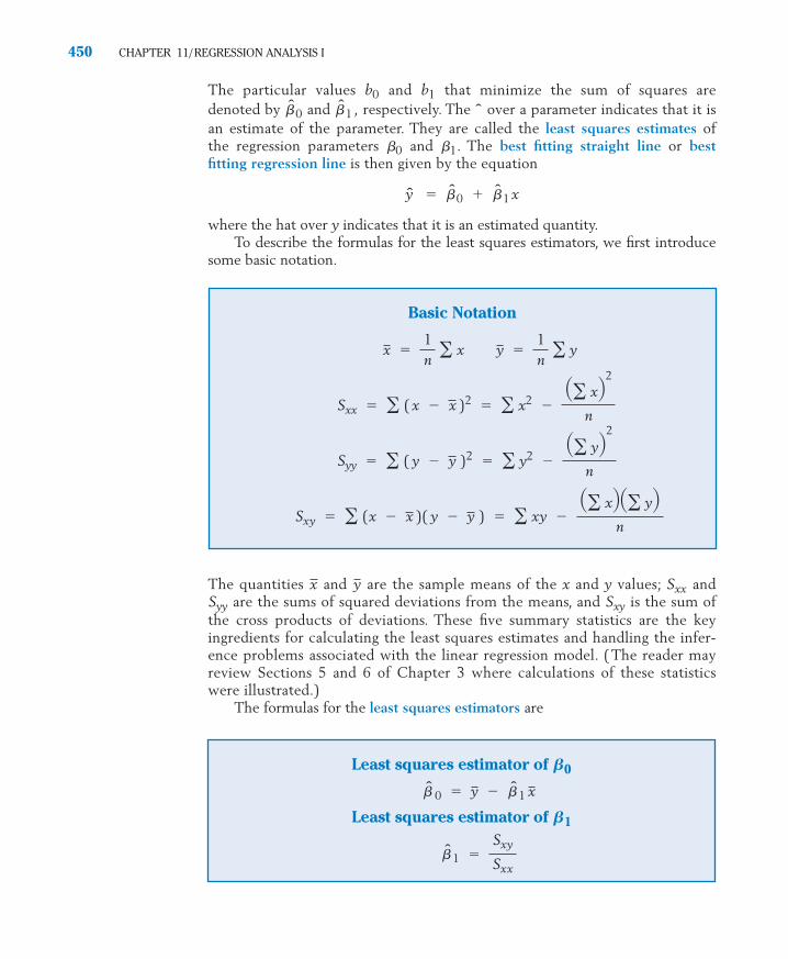
The particular values and that minimize the sum of squares are denoted by and respectively. The over a parameter indicates that it isan estimate of the parameter. They are called the least squares estimates ofthe regression parameters and . The best fitting straight line or bestfitting regression line is then given by the equation
where the hat over y indicates that it is an estimated quantity.To describe the formulas for the least squares estimators, we first introduce
some basic notation.
The quantities and are the sample means of the x and y values; andare the sums of squared deviations from the means, and is the sum of
the cross products of deviations. These five summary statistics are the keyingredients for calculating the least squares estimates and handling the infer-ence problems associated with the linear regression model. ( The reader mayreview Sections 5 and 6 of Chapter 3 where calculations of these statisticswere illustrated.)
The formulas for the least squares estimators are
SxySyy
Sxxyx
y � �0 � �1 x
�1�0
ˆ�1 ,�0
b1b0
450 CHAPTER 11/REGRESSION ANALYSIS I
Basic Notation
Sx y � � (x � x )( y � y ) � � x y ��� x��� y�
n
Syy � � ( y � y )2 � � y2 ��� y�
2
n
Sxx � � ( x � x )2 � � x2 ��� x�
2
n
x �1n
� x y �1n
� y
Least squares estimator of
Least squares estimator of
� 1 �Sx y
Sx x
�1
� 0 � y � � 1 x
�0
c11.qxd 10/15/09 11:16 AM Page 450

The estimates and can then be used to locate the best fitting line:
As we have already explained, this line provides the best fit to the data in thesense that the sum of squares of the deviations, or
is the smallest.The individual deviations of the observations from the fitted values
are called the residuals, and we denote these by
Some residuals are positive and some negative, and a property of the leastsquares fit is that the sum of the residuals is always zero.
In Chapter 12, we will discuss how the residuals can be used to check theassumptions of a regression model. For now, the sum of squares of the residualsis a quantity of interest because it leads to an estimate of the variance of theerror distributions illustrated in Figure 3. The residual sum of squares is alsocalled the sum of squares due to error and is abbreviated as SSE.
The second expression for SSE, which follows after some algebraic manipula-tions (see Exercise 11.24), is handy for directly calculating SSE. However, westress the importance of determining the individual residuals for their role inmodel checking (see Section 4, Chapter 12).
An estimate of variance is obtained by dividing SSE by n � 2. Thereduction by 2 is because two degrees of freedom are lost from estimating thetwo parameters and .�1�0
�
2
�
2
e i .y i � �0 � �1x i
y i
�n
i � 1 ( yi � �0 � �1x i
)
2
� 1� 0
4. THE METHOD OF LEAST SQUARES 451
Fitted (or estimated) regression line
y � � 0 � � 1
x
Residuals
e i � y i � �0 � �1
x i i � 1, . . . , n
The residual sum of squares or the sum of squares due to error is
SSE � �n
i � 1 e i
2 � Sy y �Sx y
2
Sx x
c11.qxd 10/15/09 11:16 AM Page 451

In applying the least squares method to a given data set, we first computethe basic quantities , , and . Then the preceding formulas can beused to obtain the least squares regression line, the residuals, and the value ofSSE. Computations for the data given in Table 1 are illustrated in Table 3.
Sx ySy ySx xx , y ,
452 CHAPTER 11/REGRESSION ANALYSIS I
TABLE 3 Computations for the Least Squares Line, SSE, and Residuals Using the Data of Table 1
x y xy Residual
3 9 9 81 27 7.15 1.853 5 9 25 15 7.15 �2.154 12 16 144 48 9.89 2.115 9 25 81 45 12.63 �3.636 14 36 196 84 15.37 �1.376 16 36 256 96 15.37 .637 22 49 484 154 18.11 3.898 18 64 324 144 20.85 �2.858 24 64 576 192 20.85 3.159 22 81 484 198 23.59 �1.59
Total 59 151 389 2651 1003 .04 (rounding error)
Sx y � 1003 �
59 � 15110
� 112.1
SSE � 370.9 �(112.1)2
40.9� 63.6528Sy y � 2651 �
(151)2
10� 370.9
�0 � 15.1 � 2.74 � 5.9 � �1.07Sx x � 389 �(59)2
10� 40.9
�1 �112.140.9
� 2.74y � 15.1x � 5.9,
e� 0 � � 1xy
2x2
Estimate of Variance
The estimator of the error variance is
S2 �SSE
n � 2
�
2
The data in the first two columns yield the next three columns. Then, the sumof entries in a column are obtained so , , and can be calculated.From these, , and SSE are obtained.� 0, � 1
Sx ySy ySx xx , y ,
c11.qxd 10/15/09 11:16 AM Page 452
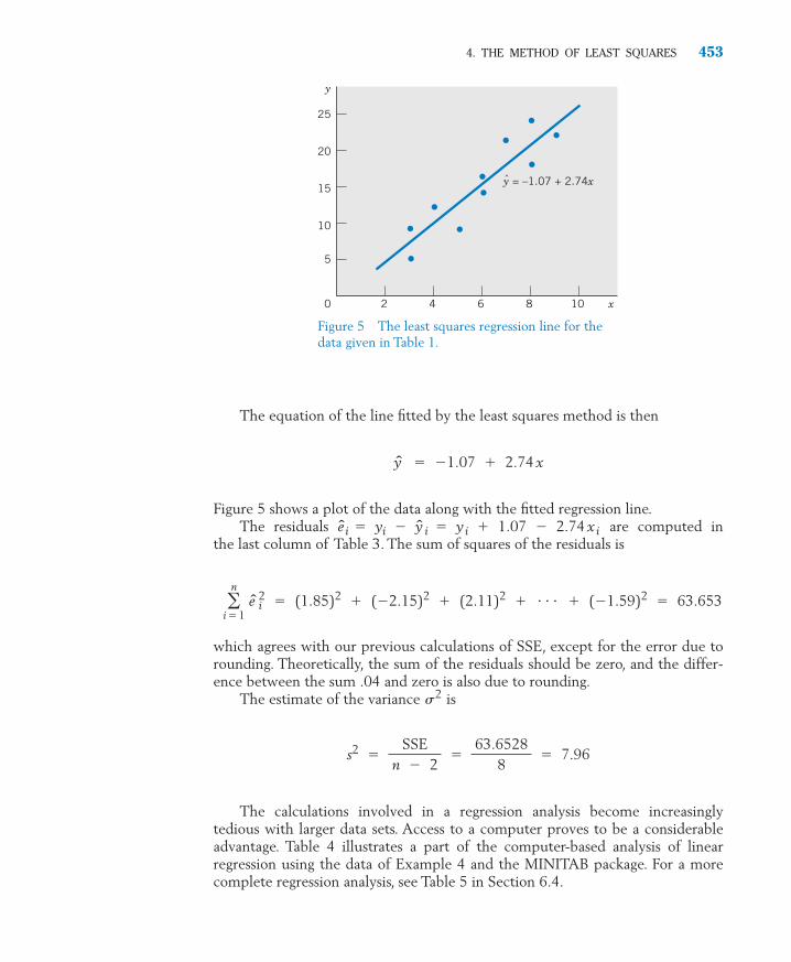
4. THE METHOD OF LEAST SQUARES 453
y = –1.07 + 2.74x
y
25
20
15
10
5
0 2 4 6 8 10 x
Figure 5 The least squares regression line for thedata given in Table 1.
The equation of the line fitted by the least squares method is then
Figure 5 shows a plot of the data along with the fitted regression line.The residuals are computed in
the last column of Table 3. The sum of squares of the residuals is
which agrees with our previous calculations of SSE, except for the error due torounding. Theoretically, the sum of the residuals should be zero, and the differ-ence between the sum .04 and zero is also due to rounding.
The estimate of the variance is
The calculations involved in a regression analysis become increasinglytedious with larger data sets. Access to a computer proves to be a considerableadvantage. Table 4 illustrates a part of the computer-based analysis of linearregression using the data of Example 4 and the MINITAB package. For a morecomplete regression analysis, see Table 5 in Section 6.4.
s2 �SSE
n � 2�
63.65288
� 7.96
�
2
�n
i � 1 e i
2 � (1.85)2 � (�2.15)2 � (2.11)2 � � � � � (�1.59)2 � 63.653
e i � yi � y i � y i � 1.07 � 2.74 x i
y � �1.07 � 2.74 x
c11.qxd 10/15/09 11:16 AM Page 453

Exercises
454 CHAPTER 11/REGRESSION ANALYSIS I
Data: C11T3 txt
C1: 3 3 4 5 6 6 7 8 8 9
C2: 9 5 12 9 14 16 22 18 24 22
Dialog box:
Stat Regression Regression
Type C2 in Response
Type C1 in Predictors. Click OK.
Output:
Regression Analysis
The regression equation is
y � �1.07 � 2.74x
TABLE 4 Regression Analysis of the Data in Table 1, Example 4, Using MINITAB
11.12 A student collected data on the number oflarge pizzas consumed, y, while x students arewatching a professional football game on TV.Suppose that the data from five games are:
x 2 5 6 3 4
y 1 6 10 3 5
(a) Construct a scatter diagram.
(b) Calculate and .
(c) Calculate the least squares estimatesand
(d) Determine the fitted line and draw theline on the scatter diagram.
11.13 The office manager at a real estate firm makes apot of coffee every morning. The time before itruns out, y, in hours depends on the number ofpersons working inside that day, x. Supposethat the pairs of (x, y) values from six days are:
x 1 2 3 3 4 5
y 8 4 5 3 3 1
� 1 .� 0
Sy yx , y , Sx x , Sx y
,
(a) Plot the scatter diagram.
(b) Calculate and .
(c) Calculate the least squares estimates and
(d) Determine the fitted line and draw theline on the scatter diagram.
11.14 Refer to Exercise 11.12.
(a) Find the residuals and verify that theysum to zero.
(b) Calculate the residual sum of squares SSE by
(i) Adding the squares of the residuals.
(ii) Using the formula SSE �
(c) Obtain the estimate of .
11.15 Refer to Exercise 11.13.
(a) Find the residuals and verify that theysum to zero.
(b) Calculate the residual sums of squaresSSE by
�
2
Sx y2 / Sx xSy y �
� 1 .� 0
Sy yx , y , Sx x , Sx y
,
c11.qxd 10/15/09 11:16 AM Page 454

(i) Adding the squares of the residuals.
(ii) Using the formula SSE �
(c) Obtain the estimate of .
11.16 A help desk devoted to student software prob-lems also receives phone calls. The number ofpersons that can be served in person, withinone hour, is the response y . The predictor vari-able, x , is the number of phone calls answered.
x 0 1 2 3 4
y 7 8 5 4 1
(a) Calculate and .
(b) Calculate the least squares estimates and
(c) Determine the fitted line.
(d) Use the fitted line to predict the number ofpersons served when 3 calls are answered.
�1 .�0
Sy yx , y , Sx x , Sx y
,
�
2
Sx y2 / Sx xSy y �
4. THE METHOD OF LEAST SQUARES 455
11.17 A student hourly employee does small secretar-ial projects. The number of projects she com-pletes in a day is the response variable y. Thenumber of hours she works in a day is the pre-dictor variable x.
x 1 2 4 6 7
y 4 3 6 8 9
(a) Calculate and .
(b) Calculate the least squares estimates and
(c) Determine the fitted line.(d) Use the fitted line to predict the number
of projects completed when she works 6.5hours.
11.18 Crime is becoming more of a problem onmany college campuses. The U.S. Departmentof Education reports data on alleged crimes atuniversities and colleges. Table 5 gives the data
�1 .�0
Sy yx , y , Sx x , Sx y
,
TABLE 5 Crime at the Largest Universities
Enrollment ForcibleUniversity (1000) Rape Robbery Burglary Arson
Ohio State 52.57 65 11 212 17Minnesota 50.88 12 7 272 3Central Florida 48.40 3 1 43 0Michigan State 46.05 18 11 122 1Pennsylvania State 43.25 8 3 112 7Wisconsin-Madison 41.56 7 5 167 6Florida State 40.56 10 8 69 3Washington-Seattle 40.22 0 3 70 3Florida International 38.18 3 5 90 1Arizona 37.22 8 0 43 0San Diego State 35.70 10 4 61 1California-Berkeley 34.94 4 24 74 11Rutgers-New Brunswick 34.80 4 4 97 5Georgia 33.83 1 0 17 0Boston 32.05 7 1 62 0North Carolina State-Raleigh 31.80 6 8 57 1San Francisco State 30.13 9 1 45 1Purdue University-Indianapolis 29.85 1 0 93 0California-Davis 29.80 7 9 42 2Iowa 29.12 6 1 36 1
c11.qxd 10/15/09 11:16 AM Page 455

from the year 2007, for the twenty universitieswith the largest enrollments.
When y is the number of burglaries and thepredictor variable x is enrollment, we have
(a) Obtain the equation of the best fittingstraight line.
(b) Calculate the residual sum of squares.
(c) Estimate .
11.19 Refer to the crime data in Exercise 11.18, Table 5.
When y is the number of robberies and thepredictor variable x is arson incidents, we have
(a) Obtain the equation of the best fittingstraight line.
(b) Calculate the residual sum of squares.
(c) Estimate .
11.20 The data on female wolves in Table D.9 of theData Bank concerning body weight ( lb) andbody length (cm) are
Weight 57 84 90 71 77 68 73
Body length 123 129 143 125 122 125 122
(a) Obtain the least squares fit of bodyweight to the predictor body length.
(b) Calculate the residual sum of squares.
(c) Estimate .� 2
� 2
Sx x � 358.55 Sx y � 290.10 Sy y � 618.2 n � 20 x � 3.15 y � 5.30
� 2
Sx x � 994.038 Sx y � 6191.04 Sy y � 76,293.2 n � 20 x � 38.046 y � 89.20
456 CHAPTER 11/REGRESSION ANALYSIS I
5. THE SAMPLING VARIABILITY OF THE LEAST SQUARES ESTIMATORS—TOOLS FOR INFERENCE
It is important to remember that the line obtained by theprinciple of least squares is an estimate of the unknown true regression line y �
In our drug evaluation problem (Example 4), the estimated line is
Its slope suggests that the mean duration of relief increases by 2.74hours for each unit dosage of the drug. Also, if we were to estimate the expectedduration of relief for a specified dosage milligrams, we would naturallyx* � 4.5
�1 � 2.74
y � �1.07 � 2.74 x
�0 � �1 x.
y � �0 � �1 x
11.21 Refer to the data on female wolves in Exercise11.20.
(a) Obtain the least squares fit of body lengthto the predictor body weight.
(b) Calculate the residual sum of squares.
(c) Estimate .
(d) Compare your answer in part (a) withyour answer to part (a) of Exercise 11.20.Should the two answers be the same?Why or why not?
11.22 Using the formulas of and SSE, show thatSSE can also be expressed as
(a)
(b)
11.23 Referring to the formulas of and showthat the point lies on the fitted regres-sion line.
11.24 To see why the residuals always sum to zero,refer to the formulas of and and verifythat
(a) The predicted values are
(b) The residuals are
Then show that
(c) Verify that
2 �1 Sx y � Sy y � Sx y
2 / Sx x .
�n
i � 1 e i
2 � Sy y � � 12 Sx x �
�n
i � 1 e i � 0.
( yi � y ) � �1( xi � x )e i � yi � y i �
�1( xi � x ) .y i � y �
�1 �0
( x , y )�1 ,�0
SSE � Syy � �12 Sxx
SSE � Syy � �1Sxy
�1
� 2
c11.qxd 10/15/09 11:16 AM Page 456

5. THE SAMPLING VARIABILITY OF THE LEAST SQUARES ESTIMATORS—TOOLS FOR INFERENCE 457
1. The standard deviations (also called standard errors) of the leastsquares estimators are
To estimate the standard error, use
S � �
SSEn � 2
in place of �
S.E.( �1) ��
√ Sx x
S.E.( � 0) � � � 1n
�x2
Sx x
2. Inferences about the slope are based on the t distribution
Inferences about the intercept are based on the t distribution
T ��0 � �0
S �
1n
�x2
Sx x
d.f. � n � 2
�0
T ��1 � �1
S / √ Sx x
d.f. � n � 2
�1
3. At a specified value the expected response is � x*.This is estimated by with
Estimated standard error
S �
1n
�(x* � x )2
Sx x
�0 � �1 x*�1�0x � x*,
use the fitted regression line to calculate the estimate 11.26 days. A few questions concerning these estimates naturally arise at this point.
1. In light of the value 2.74 for could the slope of the true regres-sion line be as much as 4? Could it be zero so that the true regressionline is which does not depend on x? What are the plausiblevalues for ?
2. How much uncertainty should be attached to the estimated duration of11.26 days corresponding to the given dosage
To answer these and related questions, we must know something about thesampling distributions of the least squares estimators. These sampling distributionswill enable us to test hypotheses and set confidence intervals for the parameters
and that determine the straight line and for the straight line itself. Again, thet distribution is relevant.
�1�0
x* � 4.5?
�1
y � �0 ,
�1�1 ,
�1.07 � 2.74 � 4.5 �
c11.qxd 10/15/09 11:16 AM Page 457

6. IMPORTANT INFERENCE PROBLEMS
We are now prepared to test hypotheses, construct confidence intervals, andmake predictions in the context of straight line regression.
6.1. INFERENCE CONCERNING THE SLOPE
In a regression analysis problem, it is of special interest to determine whetherthe expected response does or does not vary with the magnitude of the inputvariable x. According to the linear regression model,
Expected response � � x
This does not change with a change in x if and only if � 0. We can thereforetest the null hypothesis � � 0 against a one- or a two-sided alternative,depending on the nature of the relation that is anticipated. If we refer to theboxed statement (2) of Section 5, the null hypothesis � � 0 is to betested using the test statistic
Example 5 A Test to Establish That Duration of Relief Increases with DosageDo the data given in Table 1 constitute strong evidence that the mean dura-tion of relief increases with higher dosages of the drug?
SOLUTION For an increasing relation, we must have � 0. Therefore, we are to test the null hypothesis � � 0 versus the one-sided alternative � � 0.We select � .05. Since � 1.860, with d.f. � 8 we set the rejection region R�T 1.860. Using the calculations that follow Table 3, we have
s
2 �SSE
n � 2�
63.65288
� 7.9566, s � 2.8207
�1 � 2.74
t.05
�1H1�1H0
�1
T ��1
S / √Sx x
d.f. � n � 2
�1H0
�1H0
�1
�1�0
�1
458 CHAPTER 11/REGRESSION ANALYSIS I
Inferences about � x* are based on the t distribution
T �( � 0 � �1 x* ) � ( �0 � �1 x* )
S �
1n
�( x* � x )2
Sx x
d.f. � n � 2
�1�0
c11.qxd 10/15/09 11:16 AM Page 458

The observed t value is in the rejection region, so is rejected. Moreover, 6.213is much larger than � 3.355, so the P–value is much smaller than .005.
A computer calculation gives There is strongevidence that larger dosages of the drug tend to increase the duration of reliefover the range covered in the study.
A warning is in order here concerning the interpretation of the test of � � 0. If is not rejected, we may be tempted to conclude that y
does not depend on x. Such an unqualified statement may be erroneous. First,the absence of a linear relation has only been established over the range of thex values in the experiment. It may be that x was just not varied enough to in-fluence y. Second, the interpretation of lack of dependence on x is valid only ifour model formulation is correct. If the scatter diagram depicts a relation on acurve but we inadvertently formulate a linear model and test � � 0,the conclusion that is not rejected should be interpreted to mean “no lin-ear relation,” rather than “no relation.” We elaborate on this point further inSection 7. Our present viewpoint is to assume that the model is correctly for-mulated and discuss the various inference problems associated with it.
More generally, we may test whether or not is equal to some specifiedvalue , not necessarily zero.�10
�1
H0
�1H0
H0�1H0
P[T � 6.213] � .0001.t.005
H0
Test statistic t �2.74.441
� 6.213
Estimated S.E.( �1
) �s
√ Sx x
�2.8207
√40.90� .441
6. IMPORTANT INFERENCE PROBLEMS 459
The test of the null hypothesis
is based on
T ��1 � �10
S / √ Sxx
d.f. � n � 2
H0 : �1 � �10
A 100(1 � )% confidence interval for is
where is the upper /2 point of the t distribution with d.f. � n � 2.t�2
� �1 � t / 2 S
√ Sxx
, �1 � t / 2 S
√ Sx x
��1
In addition to testing hypotheses, we can provide a confidence interval forthe parameter using the t distribution.�1
c11.qxd 10/15/09 11:16 AM Page 459
Example 6 A Confidence Interval for Construct a 95% confidence interval for the slope of the regression line inreference to the drug trial data of Table 1.
SOLUTION In Example 5, we found that and The requiredconfidence interval is given by
We are 95% confident that by adding one extra milligram to the dosage, themean duration of relief would increase somewhere between 1.72 and 3.76 hours.
6.2. INFERENCE ABOUT THE INTERCEPT
Although somewhat less important in practice, inferences similar to those out-lined in Section 6.1 can be provided for the parameter . The procedures are again based on the t distribution with d.f. � n � 2, stated for in Section 5.In particular,
To illustrate this formula, let us consider the data of Table 1. In Table 3, wehave found and Also,Therefore, a 95% confidence interval for is calculated as
Note that represents the mean response corresponding to the value 0 for the input variable x. In the drug evaluation problem of Example 4, the parameter isof little practical interest because the range of x values covered in the experimentwas 3 to 9 and it would be unrealistic to extend the line to In fact, the esti-mate does not have an interpretation as a (time) duration of relief.
6.3. ESTIMATION OF THE MEAN RESPONSE FOR A SPECIFIED x VALUE
Often, the objective in a regression study is to employ the fitted regression inestimating the expected response corresponding to a specified level of the inputvariable. For example, we may want to estimate the expected duration of relief fora specified dosage x* of the drug. According to the linear model described in
�0 � �1.07x � 0.
� 0
� 0
� �1.07 � 6.34 or ( �7.41, 5.27 )
�1.07 � 2.306 � 2.8207 � 110
�( 5.9 )2
40.9
� 0
s � 2.8207.Sx x � 40.9.x � 5.9,�0 � �1.07,
�0
� 0
�0
2.74 � 2.306 � .441 � 2.74 � 1.02 or (1.72, 3.76)
s / √Sx x � .441.�1 � 2.74
�1
460 CHAPTER 11/REGRESSION ANALYSIS I
A 100(1 � )% confidence interval for is
� �0 � t / 2 S � 1n
�x2
Sx x , �0 � t / 2 S � 1
n�
x2
Sxx �
� 0
c11.qxd 10/15/09 11:16 AM Page 460

Section 3, the expected response at a value x* of the input variable x is givenby � . The expected response is estimated by � which is theordinate of the fitted regression line at Referring to statement (3) ofSection 5, we determine that the t distribution can be used to construct confi-dence intervals or test hypotheses.
Example 7 A Confidence Interval for the Expected Duration of ReliefAgain consider the data given in Table 1 and the calculations for the regressionanalysis given in Table 3. Obtain a 95% confidence interval for the expectedduration of relief when the dosage is (a) and (b)
SOLUTION (a) The fitted regression line is
The expected duration of relief corresponding to the dosage mil-ligrams of the drug is estimated as
A 95% confidence interval for the mean duration of relief with the dosageis therefore
We are 95% confident that 6 milligrams of the drug produces an averageduration of relief that is between about 13.31 and 17.43 hours.
� 15.37 � 2.06 or ( 13.31, 17.43 )15.37 � t.025 � .893 � 15.37 � 2.306 � .893
x* � 6
� 2.8207 � .3166 � .893
Estimated standard error � s � 110
�( 6 � 5.9 )2
40.9
�0 � �1 x* � �1.07 � 2.74 � 6 � 15.37 hours
x* � 6
y � �1.07 � 2.74x
x* � 9.5.x* � 6
x � x*.�1 x*�0�1 x*�0
6. IMPORTANT INFERENCE PROBLEMS 461
A 100(1 � )% confidence interval for the expected response � is
�0 � �1 x* � t / 2 S � 1n
�( x* � x )2
Sx x
�1 x*�0
To test the hypothesis that � � , some specified value, we use
T ��0 � �1
x* � 0
S � 1n
�( x* � x )2
Sx x
d.f. � n � 2
0�1 x*�0
c11.qxd 10/15/09 11:16 AM Page 461

(b) Suppose that we also wish to estimate the mean duration of relief under thedosage We follow the same steps to calculate the point estimate.
A 95% confidence interval is
We are 95% confident that 9.5 milligrams of the drug produces an average of 20.76 to 29.16 hours of relief. Note that the interval is muchlarger than the one for 6 milligrams.
The formula for the standard error shows that when x* is close to the stan-dard error is smaller than it is when x* is far removed from This is confirmed byExample 7, where the standard error at x* � 9.5 can be seen to be more thantwice as large as the value at x* � 6. Consequently, the confidence interval forthe former is also wider. In general, estimation is more precise near the mean than it is for values of the x variable that lie far from the mean.
Caution concerning extrapolation: Extreme caution should be exercised inextending a fitted regression line to make long-range predictions far away fromthe range of x values covered in the experiment. Not only does the confidenceinterval become so wide that predictions based on it can be extremely unreli-able, but an even greater danger exists. If the pattern of the relationship be-tween the variables changes drastically at a distant value of x, the data provideno information with which to detect such a change. Figure 6 illustrates this sit-uation. We would observe a good linear relationship if we experimented withx values in the 5 to 10 range, but if the fitted line were extended to estimatethe response at x* � 20, then our estimate would drastically miss the mark.
x
x.x ,
24.96 � 2.306 � 1.821 � 24.96 � 4.20 or ( 20.76, 29.16 )
� 1.821
Estimated standard error � 2.8207 � 110
�( 9.5 � 5.9 )2
40.9
�0 � �1x* � �1.07 � 2.74 � 9.5 � 24.96 days
x* � 9.5.
462 CHAPTER 11/REGRESSION ANALYSIS I
Predicted
True relation
y
5 10 20 x
Figure 6 Danger in long-range prediction.
c11.qxd 10/15/09 11:16 AM Page 462

6.4. PREDICTION OF A SINGLE RESPONSE FOR A SPECIFIED x VALUE
Suppose that we give a specified dosage x* of the drug to a single patient and wewant to predict the duration of relief from the symptoms of allergy. This problemis different from the one considered in Section 6.3, where we were interested inestimating the mean duration of relief for the population of all patients given thedosage x*. The prediction is still determined from the fitted line; that is, the pre-dicted value of the response is as it was in the preceding case. How-ever, the standard error of the prediction here is larger, because a single observationis more uncertain than the mean of the population distribution. We now give theformula of the estimated standard error for this case.
The formula for the confidence interval must be modified accordingly. We callthe resulting interval a prediction interval because it pertains to a futureobservation.
Example 8 Calculating a Prediction Interval for a Future TrialOnce again, consider the drug trial data given in Table 1. A new trial is to bemade on a single patient with the dosage x* � 6.5 milligrams. Predict theduration of relief and give a 95% prediction interval for the duration of relief.
SOLUTION The predicted duration of relief is
Since with d.f. � 8, a 95% prediction interval for the newpatient’s duration of relief is
This means we are 95% confident that this particular patient will have relieffrom symptoms of allergy for about 9.9 to 23.6 hours.
In the preceding discussion, we have used the data of Example 4 to illus-trate the various inferences associated with a straight-line regression model.Example 9 gives applications to a different data set.
� 16.74 � 6.85 or ( 9.89, 23.59 )
16.74 � 2.306 � 2.8207 � 1 �1
10�
( 6.5 � 5.9 )2
40.9
t.025 � 2.306
�0 � �1 x* � �1.07 � 2.74 � 6.5 � 16.74 hours
�0 � �1 x*
6. IMPORTANT INFERENCE PROBLEMS 463
The estimated standard error when predicting a single observation y at agiven x* is
S � 1 �1n
�( x* � x )2
Sx x
c11.qxd 10/15/09 11:16 AM Page 463

Example 9 Prediction after Fitting a Straight Line Relation of a HumanDevelopment Index to Internet UsageOne measure of the development of a country is the Human DevelopmentIndex (HDI) which combines life expectancy, literacy, educational attain-ment, and gross domestic product per capita into an index whose values liebetween 0 and 1, inclusive.
We randomly selected fifteen countries, of the 152 countries, below thetop twenty-five most developed countries on the list. HDI is the responsevariable y , and Internet usage per 100 persons, x , is the predictor variableThe data, given in Exercise 11.31, have the summary statistics
n = 15 = 9.953 = .6670
(a) Determine the equation of the best fitting straight line.
(b) Do the data substantiate the claim that Internet usage per 100 per-sons is a good predictor of HDI and that large values of both vari-ables tend to occur together?
(c) Estimate the mean value of HDI for 18 Internet users per 100 per-sons and construct a 95% confidence interval.
(d) Find the predicted y for x = 43 Internet users per 100 persons.
SOLUTION
(a)
So, the equation of the fitted line is
(b) To answer this question, we decide to test : = 0 versus : >0.The test statistic is
We select � .01. Since with d.f. � 13, we set the right-sided rejection region R�T ≥ 2.650. We calculate
SSE � Sy y �Sx y
2
Sx x� .41772 �
( 20.471)2
1173.46� .06060
t.01 � 2.650
T ��1
S / √ Sx x
�1H1�1H0
y � .493 � .0174x
�0 � y � �1 x � .6670 � .017445 � 9.953 � .4934
�1 �Sx y
Sx x�
20.4711173.46
� .017445
Sx x � 1173.46 Sy y � 20.471 Sx y � .41772 yx
464 CHAPTER 11/REGRESSION ANALYSIS I
c11.qxd 10/15/09 11:16 AM Page 464
The t statistic has the value
Since the observed is greater than 2.650, is rejected with � .01. The P–value is much less than .0001.
We conclude that larger values of Internet users per 100 persons signifi-cantly increases the expected HDI, within the range of values of x includedin the data.
(c) The expected value of the HDI corresponding to x* = 18 Internet usersper 100 is estimated as
and its
Since for d.f. � 13, the required confidence interval is
We are 95% confident that the expected value of HDI, for x* = 18, is between.756 and .859.
(d) Since is far above the largest value of 26.2 users per 100, it isnot sensible to predict y at x = 43 using the fitted regression line. Here aformal calculation gives
which is a nonsensical result for an index that should not exceed 1. As men-tioned earlier, extrapolation typically gives unreliable results.
Regression analyses are most conveniently done on a computer. A morecomplete selection of the output from the computer software packageMINITAB, for the data in Example 4, is given in Table 6.
Predicted HDI � .4934 � .01745( 43 ) � 1.244
x � 43
.8075 � 2.160 � .0238 � .8075 � .0514 or ( .756, .859 )
t.025 � 2.160
Estimated S.E. � s �
115
�(18 � 9.953)2
1173.46� .0238
�0 � �1 x* � .4934 � .01745(18 ) � .8075
H0t � 8.77
t �.01744.00199
� 8.77
Estimated S.E. ( �1) �s
√ Sx x
�.0683
√ 1173.46� .00199
s � �
SSEn � 2
� �
.0606013
� .0683
6. IMPORTANT INFERENCE PROBLEMS 465
c11.qxd 10/15/09 11:16 AM Page 465

466 CHAPTER 11/REGRESSION ANALYSIS I
TABLE 7 SAS Computer Output for the Data in Example 4
MODEL: MODEL 1DEPENDENT VARIABLE: Y
ANALYSIS OF VARIANCE
SUM OF MEANSOURCE DF SQUARES SQUARE F VALUE PROB � F
MODEL 1 307.24719 307.24719 38.615 0.0003ERROR 8 63.65281 7.95660C TOTAL 9 370.90000
ROOT MSE 2.82074 R-SQUARE 0.8284
PARAMETER ESTIMATES
PARAMETER STANDARD T FOR HO:VARIABLE DF ESTIMATE ERROR PARAMETER � 0 PROB
INTERCEP 1 �1.070905 2.75091359 �0.389 0.7072X1 1 2.740831 0.44106455 6.214 0.0003
� � T �
The output of the computer software package SAS for the data in Example 4is given in Table 7. Notice the similarity of information in Tables 6 and 7. Bothinclude the least squares estimates of the coefficients, their estimated standarddeviations, and the t test for testing that the coefficient is zero. The estimate of is presented as the mean square error in the analysis of variance table.
�
2
TABLE 6 MINITAB Computer Output for the Data in Example 4
THE REGRESSION EQUATION ISY � �1.07 � 2.74X
PREDICTOR COEF STDEV T-RATIO PCONSTANT �1.071 2.751 �0.39 0.707X 2.7408 0.4411 6.21 0.000
S � 2.821 R-SQ � 82.8%
ANALYSIS OF VARIANCE
SOURCE DF SS MS F PREGRESSION 1 307.25 307.25 38.62 0.000ERROR 8 63.65 7.96TOTAL 9 370.90
c11.qxd 10/15/09 11:16 AM Page 466

Example 10 Predicting the Number of Situps after a Semester of ConditioningUniversity students taking a physical fitness class were asked to count thenumber of situps they could do at the start of the class and again at the endof the semester.
Refer to the physical fitness data, on numbers of situps, in Table D.5 ofthe Data Bank.
(a) Find the least squares fitted line to predict the posttest number ofsitups from the pretest number at the start of the conditioning class.
(b) Find a 95% confidence interval for the mean number of posttest situpsfor persons who can perform 35 situps in the pretest. Also find a 95%prediction interval for the number of posttest situps that will be per-formed by a new person this semester who does 35 situps in thepretest.
(c) Repeat part (b), but replace the number of pretest situps with 20.
SOLUTION The scatter plot in Figure 7 suggests that a straight line may model theexpected value of posttest situps given the number of pretest situps. Here x isthe number of pretest situps and y is the number of posttest situps. We useMINITAB statistical software to obtain the output
Regression Analysis: Post Situps versus Pre Situps
The regression equation isPost Situps = 10.3 � 0.899 Pre Situps
Predictor Coef SE Coef T PConstant 10.331 2.533 4.08 0.000Pre Situps 0.89904 0.06388 14.07 0.000
S � 5.17893 R-Sq � 71.5%
Analysis of Variance
Source DF SS MS F PRegression 1 5312.9 5312.9 198.09 0.000Residual Error 79 2118.9 26.8Total 80 7431.8
Predicted Values for New Observations
NewObs Pre Sit Fit SE Fit 95% CI 95% PI1 35.0 41.797 0.620 (40.563, 43.032) (31.415, 52.179)2 20.0 28.312 1.321 (25.682, 30.941) (17.673, 38.950)
From the output and �
� 26.8 is the estimate of .�
2( 5.1789 )
2s
2y � �0 � �1x � 10.3 � 0.899 x
6. IMPORTANT INFERENCE PROBLEMS 467
c11.qxd 10/15/09 11:16 AM Page 467

We have selected the option in MINITAB to obtain the two confi-dence intervals and prediction intervals given in the output. The predic-tion intervals pertain to the posttest number of situps performed by a specific new person. The first is for a person who performed 35 situps in the pretest. The prediction intervals are wider than the correspondingconfidence intervals for the expected number of posttest situps for the population of all students who would do 35 situps in the pretest. The same relation holds, as it must, for 20 pretest situps.
Exercises
468 CHAPTER 11/REGRESSION ANALYSIS I
11.25 We all typically go to the shortest line in thegrocery store. Data were collected on the num-ber of carts ahead in line and the total time tocheck out (minutes), including time in line, onfive occasions.
(a) Calculate the least squares estimates and Also estimate the error variance .
(b) Test � � 0 versus � � 0with � .05.
(c) Estimate the expected y value corre-sponding to carts and give a 90%confidence interval.
11.26 Refer to Exercise 11.25. Construct a 90%confidence interval for the intercept . Inter-pret.
11.27 Refer to Exercise 11.25. Obtain a 95% confi-dence interval for . Interpret.�1
� 0
x � 3
�1H1�1H0
�
2�1 .�0
Number Time to of Carts Check Out
1 52 113 94 145 16
70
60
50
40
30
20
20 30 40 50 60
Pos
ttes
t S
itup
s
Pretest Situps
Figure 7 Scatter plot of number of situps.
c11.qxd 10/15/09 11:16 AM Page 468

11.28 An engineer found that by adding smallamounts of a compound to rechargeable bat-teries during manufacture, she could extendtheir lifetimes. She experimented with differ-ent amounts of the additive ( g ) and measuredthe hours they lasted in a laptop.
(a) Calculate the least squares estimates and Also estimate the error
variance .
(b) Test : � 1 versus � � 1with � .05.
(c) Estimate the expected y value corre-sponding to and give a 95%confidence interval. Interpret.
(d) Construct a 90% confidence interval forthe intercept . Interpret.
11.29 For a random sample of seven homes that arerecently sold in a city suburb, the assessedvalues x and the selling prices y are
(a) Plot the scatter diagram.(b) Determine the equation of the least
squares regression line and draw this lineon the scatter diagram.
(c) Construct a 95% confidence interval forthe slope of the regression line. Interpret.
11.30 Refer to the data in Exercise 11.29.(a) Estimate the expected selling price of homes
that were assessed at $290,000 and con-struct a 95% confidence interval. Interpret.
(b) For a single home that was assessed at$290,000, give a 95% prediction intervalfor the selling price. Interpret.
�0
x � 3.5
�1H1�1H0
�
2�1 .�0
11.31 One measure of the development of a countryis the Human Development Index (HDI). Lifeexpectancy, literacy, educational attainment,and gross domestic product per capita arecombined into an index between 0 and 1, in-clusive with 1 being the highest development.The United Nations Development Program re-ports values for 177 countries. We randomlyselected fifteen countries, below the toptwenty-five. Both HDI and the predictor vari-able x = Internet usage per 100 persons are ob-tained from their reports.
6. IMPORTANT INFERENCE PROBLEMS 469
Amount Life of Additive (hours)
0 1.91 2.02 2.53 2.64 3.0
($1000)x y
283.5 288.0290.0 291.2270.5 276.2300.8 307.0
($1000)x y
310.2 311.0294.6 299.0320.0 318.0
TABLE 8 Human Development Index
Country Internet/100 HDI
Bahrain 21.3 .866Poland 26.2 .870Uruguay 14.3 .852Bulgaria 20.6 .824Brazil 19.5 .800Ukraine 9.7 .788Dominican Republic 16.9 .799Moldova 9.6 .708India 5.5 .619Madagascar 0.5 .533Nepal 0.4 .534Tanzania 0.9 .467Uganda 1.7 .505Zambia 2.0 .434Ethiopia 0.2 .406
Source: Human Development 2007–2008 reports atUNDP web site http://hdr.undp.org
n = 15 = 9.953 = .6670
(a) Obtain a 95% confidence interval for themean HDI when Internet usage per 100 per-sons is 22. Compare the width of the intervalwith that of the interval in Example 9.
(b) Obtain a 95% prediction interval for a singlecountry with Internet usage 22 per one hun-dred persons. Interpret.
(c) Does your analysis show that Internet avail-ability causes HDI to increase?
Sx x � 1173.46 Sx y � 20.471 Sy y � .41772 yx
c11.qxd 10/15/09 11:16 AM Page 469

470 CHAPTER 11/REGRESSION ANALYSIS I
11.32 Refer to Exercise 11.31.
(a) Obtain the least squares estimates by fit-ting a straight line to the response Inter-net usage using the predictor variableHDI.
(b) Test, with = .05, : = 0 versus atwo-sided alternative.
(c) Obtain a 95% confidence interval for themean Internet usage per 100 persons,when the HDI is .650. Interpret.
(d) Obtain a 95% prediction interval for Inter-net usage in a single country with HDI.650. Interpret.
11.33 According to the computer output in Table 9:
(a) What model is fitted?
(b) Test, with � .05, if the x term isneeded in the model.
11.34 According to the computer output in Table 9:
(a) Predict the mean response when
(b) Find a 90% confidence interval forthe mean response when You will need the additional informationn � 30, x � 8354, and
( � x ) � 97,599,296.2xi�
x � 5000.
x � 5000.
�1H0
TABLE 9 Computer Output for Exercises 11.33 and 11.34
THE REGRESSION EQUATION ISY � 994 � 0.104X
PREDICTOR COEF STDEV T-RATIO PCONSTANT 994.0 254.7 3.90 0.001X 0.10373 0.02978 3.48 0.002
S � 299.4 R-SQ � 30.2%
ANALYSIS OF VARIANCE
SOURCE DF SS MS F PREGRESSION 1 1087765 1087765 12.14 0.002ERROR 28 2509820 89636TOTAL 29 3597585
11.35 According to the computer output in Table 10:
(a) What model is fitted?
(b) Test, with � .05, if the x term isneeded in the model.
11.36 According to the computer output in Table 10:
(a) Predict the mean response when
(b) Find a 90% confidence interval forthe mean response when You willneed the additional information n � 25,x � 1.793, and
(c) Find a 90% confidence interval for themean response when Interpret.
11.37 Consider the data on male wolves in Table D.9of the Data Bank concerning age (years) andcanine length (mm).
(a) Obtain the least squares fit of caninelength to the predictor age.
(b) Test � � 0 versus � � 0with � .05.
(c) Obtain a 90% confidence interval for thecanine length when age is x � 4.
(d) Obtain a 90% prediction interval for thecanine length of an individual wolf whenthe age is x � 4.
�1H1�1H0
x � 2.
� 1.848.( xi � x )2�
x � 3.
x � 3.
c11.qxd 10/15/09 11:16 AM Page 470

7. THE STRENGTH OF A LINEAR RELATION
To arrive at a measure of adequacy of the straight line model, we examine howmuch of the variation in the response variable is explained by the fitted regres-sion line. To this end, we view an observed as consisting of two components.
In an ideal situation where all the points lie exactly on the line, the residuals areall zero, and the y values are completely accounted for or explained by the lin-ear dependence on x.
We can consider the sum of squares of the residuals
to be an overall measure of the discrepancy or departure from linearity. Thetotal variability of the y values is reflected in the total sum of squares
of which SSE forms a part. The difference
Sy y � �n
i � 1 ( yi � y )2
SSE � �n
i � 1 ( yi � �0 � �1x i )2 � Sy y �
Sx y2
Sx x
y i
7. THE STRENGTH OF A LINEAR RELATION 471
TABLE 10 Computer Output for Exercises 11.35 and 11.36
THE REGRESSION EQUATION ISY � 0.338 � 0.831X
PREDICTOR COEF STDEV T-RATIO PCONSTANT 0.3381 0.1579 2.14 0.043X 0.83099 0.08702 9.55 0.000
S � 0.1208 R-SQ � 79.9%
ANALYSIS OF VARIANCE
SOURCE DF SS MS F PREGRESSION 1 1.3318 1.3318 91.20 0.000ERROR 23 0.3359 0.0146TOTAL 24 1.6676
� �
Observed Explained by Residual ory value linear relation deviation from
linear relation
( yi � �0 � � 1 x i )( �0 � �1x i
)yi
c11.qxd 10/15/09 11:16 AM Page 471

472 CHAPTER 11/REGRESSION ANALYSIS I
forms the other part. Paralleling the decomposition of the observation , as aresidual plus a part due to regression, we consider a decomposition of the vari-ability of the y values.
The first term on the right-hand side of this equality is called the sum ofsquares (SS) due to regression. Likewise, the total variability is also calledthe total SS of y. In order for the straight line model to be considered as provid-ing a good fit to the data, the SS due to the linear regression should comprise amajor portion of . In an ideal situation in which all points lie on the line, SSEis zero, so is completely explained by the fact that the x values vary in theexperiment. That is, the linear relationship between y and x is solely responsiblefor the variability in the y values.
As an index of how well the straight line model fits, it is then reasonable toconsider the proportion of the y variability explained by the linear relation
=
From Section 6 of Chapter 3, recall that the quantity
is named the sample correlation coefficient. Thus, the square of the sample cor-relation coefficient represents the proportion of the y variability explained bythe linear relation.
r �Sx y
√Sx x Sy y
SS due to linear regressionTotal SS of y
�Sx y
2 / Sx x
Sy y�
Sx y
2
Sx xSy yR2
Sy y
Sy y
Sy y
Sy y � ( Sy y � SSE ) � SSE
yi
�Sx y
2
Sx x
Sy y � SSE � Sy y � � Sy y �
Sx y2
Sx x �
Decomposition of Variability
� � SSE
Total Variability explained Residual orvariability of y by the linear relation unexplained
variability
Sx y2
Sx xSy y
c11.qxd 10/15/09 11:16 AM Page 472

Example 11 The Proportion of Variability in Duration Explained by DosageLet us consider the drug trial data in Table 1. From the calculations providedin Table 3,
Fitted regression line
How much of the variability in y is explained by the linear regression model?
SOLUTION To answer this question, we calculate
This means that 83% of the variability in y is explained by linear regression,and the linear model seems satisfactory in this respect.
Example 12 Proportion of Variation Explained in Number of SitupsRefer to physical fitness data in Table D.5 of the Data Bank. Using the dataon numbers of situps, find the proportion of variation in the posttest numberof situps explained by the pretest number that was obtained at the beginningof the conditioning class.
SOLUTION Repeating the relevant part of the computer output from Example 10,
The regression equation isPost Situps � 10.3 � 0.899 Pre Situps
Predictor Coef SE Coef T PConstant 10.331 2.533 4.08 0.000Pre Situps 0.89904 0.06388 14.07 0.000
S � 5.17893 R-Sq � 71.5%
r 2 �Sx y
2
Sx xSy y�
( 112.1 )2
40.9 � 370.9� .83
y � �1.07 � 2.74 x
Sx x � 40.9 Sy y � 370.9 Sx y � 112.1
7. THE STRENGTH OF A LINEAR RELATION 473
The strength of a linear relation is measured by
=
which is the square of the sample correlation coefficient r.
r 2 �Sx y
2
Sx x Sy yR2
The value of r is always between –1 and 1, inclusive whereas is alwaysbetween 0 and 1.
r
2
c11.qxd 10/15/09 11:16 AM Page 473

474 CHAPTER 11/REGRESSION ANALYSIS I
Analysis of Variance
Source DF SS MS F PRegression 1 5312.9 5312.9 198.09 0.000Residual Error 79 2118.9 26.8Total 80 7431.8
we find R-Sq � 71.5%, or proportion .715. From the analysis-of-variancetable we could also have calculated
Using a person’s pretest number of situps to predict their posttest number ofsitups explains that 71.5% of the variation is the posttest number.
When the value of is small, we can only conclude that a straight line rela-tion does not give a good fit to the data. Such a case may arise due to thefollowing reasons.
1. There is little relation between the variables in the sense that the scatterdiagram fails to exhibit any pattern, as illustrated in Figure 8a. In thiscase, the use of a different regression model is not likely to reduce theSSE or explain a substantial part of .Sy y
r
2
Sum of squares regressionTotal sum of squares
�5312.97431.8
� .715
y
x(a)
y
x(b)
Figure 8 Scatter diagram patterns:(a) No relation. (b) A nonlinear relation.
c11.qxd 10/15/09 11:16 AM Page 474

7. THE STRENGTH OF A LINEAR RELATION 475
2. There is a prominent relation but it is nonlinear in nature; that is, thescatter is banded around a curve rather than a line. The part of thatis explained by straight line regression is small because the model isinappropriate. Some other relationship may improve the fit substan-tially. Figure 8b illustrates such a case, where the SSE can be reduced byfitting a suitable curve to the data.
Exercises
Sy y
11.38 Refer to Exercise 11.18 and Table 5 for crimesduring the year 2007, at the twenty universi-ties with the largest enrollments. When pre-dicting number of burglaries from the predic-tor enrollment, we have
Determine the proportion of variation in y thatis explained by linear regression.
11.39 Refer to Exercise 11.20 and Table 5 for crimesduring the year 2007, at the twenty universi-ties with the largest enrollments. When y is thenumber of robberies and the predictor variablex is arson incidents, we have
n � 20� 358.55 � 290.10 � 618.2
Determine the proportion of variation in y thatis explained by linear regression.
11.40 Refer to Example 9 and Exercise 11.31, con-cerning the prediction of a human develop-ment index by Internet usage, where
n � 15� 1173.46 � 20.471 � .41772
Determine the proportion of variation in y thatis explained by linear regression.
11.41 Refer to Exercise 11.40 but consider the predic-tion of Internet usage when the human develop-ment index is the predictor variable.(a) Determine the proportion of variation in In-
ternet usage that is explained by linear re-gression.
(b) Compare your answer in Part (a) with thatof Exercise 11.40. Comment.
11.42 Refer to Exercise 11.25.(a) What proportion of the y variability is
explained by the linear regression on x?
Sy ySx ySx x
y � .6670x � 9.953
Sy ySx ySx x
y � 5.30x � 3.15
Sx x � 994.038 Sx y � 6191.04 Sy y � 76,293.2 n � 20 x � 38.046 y � 89.20
(b) Find the sample correlation coefficient.
11.43 Refer to Exercise 11.28.
(a) What proportion of y variability isexplained by the linear regression on x?
(b) Find the sample correlation coefficient.
11.44 Refer to Exercise 11.33. According to thecomputer output in Table 9, find the propor-tion of y variability explained by x. Also,calculate from the analysis of variancetable.
11.45 Refer to Exercise 11.35. According to thecomputer output in Table 10, find the propor-tion of y variability explained by x.
11.46 Consider the data on wolves in Table D.9 ofthe Data Bank concerning body length (cm)and weight ( lb). Calculate the correlationcoefficient r and for
(a) all wolves.
(b) male wolves.
(c) female wolves.
(d) Comment on the differences in your an-swers. Make a multiple scatter diagram(see Chapter 3) to clarify the situation.
*11.47 (a) Show that the sample correlation coeffi-cient r and the slope of the fittedregression line are related as
(b) Show that SSE � (1 � ) .
*11.48 Show that the SS due to regression,can also be expressed as � 1
2 Sx x .Sx y
2 / Sx x ,
Sy yr
2
r ��1 √Sx x
√Sy y
�1
r
2
R2
c11.qxd 10/15/09 11:16 AM Page 475

476 CHAPTER 11/REGRESSION ANALYSIS I
8. REMARKS ABOUT THE STRAIGHT LINE MODEL ASSUMPTIONS
A regression study is not completed by performing a few routine hypothesistests and constructing confidence intervals for parameters on the basis of theformulas given in Section 5. Such conclusions can be seriously misleading ifthe assumptions made in the model formulations are grossly incompatible withthe data. It is therefore essential to check the data carefully for indications ofany violation of the assumptions. To review, the assumptions involved in the for-mulation of our straight line model are briefly stated again.
1. The underlying relation is linear.
2. Independence of errors.
3. Constant variance.
4. Normal distribution.
Of course, when the general nature of the relationship between y andx forms a curve rather than a straight line, the prediction obtained from fittinga straight line model to the data may produce nonsensical results. Often, asuitable transformation of the data reduces a nonlinear relation to one that isapproximately linear in form. A few simple transformations are discussed inChapter 12. Violating the assumption of independence is perhaps the mostserious matter, because this can drastically distort the conclusions drawn fromthe t tests and the confidence statements associated with interval estimation.The implications of assumptions 3 and 4 were illustrated earlier in Figure 3.If the scatter diagram shows different amounts of variability in the y values fordifferent levels of x, then the assumption of constant variance may have beenviolated. Here, again, an appropriate transformation of the data often helps tostabilize the variance. Finally, using the t distribution in hypothesis testing andconfidence interval estimation is valid as long as the errors are approximatelynormally distributed. A moderate departure from normality does not impairthe conclusions, especially when the data set is large. In other words, a viola-tion of assumption 4 alone is not as serious as a violation of any of the otherassumptions. Methods of checking the residuals to detect any serious violationof the model assumptions are discussed in Chapter 12.
USING STATISTICS WISELY
1. As a first step, plot the response variable versus the predictor variable.Examine the plot to see if a linear or some other relationship exists.
2. Apply the principal of least squares to obtain estimates of the coeffi-cients when fitting a straight line model.
3. Determine the 100(1 � )% confidence intervals for the slope and in-tercept parameters. You can perform a test of hypotheses and look at
c11.qxd 10/15/09 11:16 AM Page 476

P–values to decide whether or not the parameters are zero. If not, youcan use the fitted line for prediction.
4. Don’t use the fitted line to make predictions beyond the range of thedata. The model may be different over that range.
5. Don’t assume a large , or correlation, implies a causal relationship.
KEY IDEAS AND FORMULAS
In its simplest form, regression analysis deals with studying the manner inwhich the response variable y depends on a predictor variable x. Sometimes,the response variable is called the dependent variable and predictor variable iscalled the independent or input variable.
The first important step in studying the relation between the variables y and xis to plot the scatter diagram of the data ( ), i � 1, . . . , n. If this plot indi-cates an approximate linear relation, a straight line regression model is formulated:
� � �
The random errors are assumed to be independent, normally distributed, andhave mean 0 and equal standard deviations �.
The least squares estimate and least squares estimate are obtained by the method of least squares, which minimizes the sum of squared deviations� The least squares estimates and determine thebest fitting regression line which serves to predict y from x.
The differences Observed response � Predicted response arecalled the residuals.
The adequacy of a straight line fit is measured by , which represents theproportion of y variability that is explained by the linear relation between y andx. A low value of only indicates that a linear relation is not appropriate—there may still be a relation on a curve.
Least squares estimators
Best fitting straight line
Residuals
e i � yi � y i � yi � �0 � �1 xi
y � �0 � �1 x
�1 �Sx y
Sx x �0 � y � �1 x
r
2
r
2
yi � y i �
y � �0 � �1 x ,�1�0( yi � b0 � b 1 x i )2.
�1�0
ei�1x i�0Yi
Response � A straight line in x � Random error
xi , yi
r
2
KEY IDEAS AND FORMULAS 477
c11.qxd 10/15/09 11:16 AM Page 477

478 CHAPTER 11/REGRESSION ANALYSIS I
Residual sum of squares
Estimate of variance �2
Inferences1. Inferences concerning the slope are based on the
and the sampling distribution
A 100(1 � )% confidence interval for is
To test � � , the test statistic is
2. Inferences concerning the intercept are based on the
and the sampling distribution
A 100(1 � )% confidence interval for is
�0 � t / 2 S � 1n
�x2
Sx x
�0
T ��0 � �0
S �
1n
�x2
Sx x
d.f. � n � 2
Estimated S.E. � S �
1n
�x2
Sx x
Estimator �0
�0
T ��1 � �10
S / √ Sx x
d.f. � n � 2
�10�1H0
�1 � t/2 S
√Sxx
�1
T ��1 � �1
S / √ Sx x
d.f. � n � 2
Estimated S.E. �S
√ Sx x
Estimator �1
�1
S2 �SSE
n � 2
SSE � �n
i � 1 e i
2 � Sy y �Sx y
2
Sx x
c11.qxd 10/15/09 11:16 AM Page 478

KEY IDEAS AND FORMULAS 479
3. At a specified the expected response is � x*. Inferencesabout the expected response are based on the
A 100(1 � )% confidence interval for the expected response at x* isgiven by
4. A single response at a specified is predicted by with
A 100(1 � )% prediction interval for a single response is
Decomposition of Variability
The total sum of squares is the sum of two components, the sum of squares
due to regression and the sum of squares due to error
Variability explained by the linear relation �
Residual or unexplained variability � SSE
Total y variability �
The strength of a linear relation, or proportion of y variability explained bylinear regression
Sample correlation coefficient
r �Sx y
√Sx x Sy y
r 2 �Sx y
2
Sx x Sy y
Sy y
Sx y2
Sx x� � 1
2 Sx x
Syy �S2
xy
Sxx� SSE
S2x y /Sx x
Sy y
�0 � �1 x* � t / 2 S � 1 �1n
�( x* � x )2
Sx x
Estimated S.E. � S � 1 �1n
�( x* � x )2
Sx x
�0 � �1 x*x � x*
�0 � �1 x* � t / 2 S �
1n
�( x* � x )2
Sx x
Estimated S.E. � S �
1n
�( x* � x )2
Sx x
Estimator �0 � �1 x*
�1�0x � x*,
c11.qxd 10/15/09 11:16 AM Page 479

480 CHAPTER 11/REGRESSION ANALYSIS I
TECHNOLOGY
Fitting a straight line and calculating the correlation coefficient
MINITAB
Fitting a straight line—regression analysis
Begin with the values for the predictor variable x in C1 and the response vari-able y in C2.
Stat � Regression � Regression.Type C2 in Response. Type C1 in Predictors.Click OK.
To calculate the correlation coefficient, start as above with data in C1 and C2.
Stat � Basic Statistics � Correlation.Type C1 C2 in Variables. Click OK.
EXCEL
Fitting a straight line—regression analysis
Begin with the values of the predictor variable in column A and the values ofthe response variable in column B. To plot,
Highlight the data and go to Insert and then Chart.Select XY(Scatter) and click Finish.Go to Chart and then Add Trendline.Click on the Options tab and check Display equation on chart.Click OK.
To obtain a more complete statistical analysis and diagnostic plots, instead usethe following steps:
Select Tools and then Data Analysis.Select Regression. Click OK.With the cursor in the Y Range, highlight the data in column B.With the cursor in the X Range, highlight the data in column A.Check boxes for Residuals, Residual Plots, and Line Fit Plot. Click OK.
To calculate the correlation coefficient, begin with the first variable in column Aand the second in column B.
Click on a blank cell. Select Insert and then Function(or click on the icon).Select Statistical and then CORREL.Highlight the data in column A for Array1 and highlight the data in column Bfor Array2. Click OK.
fx
c11.qxd 10/15/09 11:16 AM Page 480

TI-84/-83 PLUS
Fitting a straight line—regression analysis
Enter the values of the predictor variable in L1 and those of the response variable in L2.
Select STAT, then CALC, and then 4�LinReg (ax � b).With LinReg on the Home screen, press Enter.
The calculator will return the intercept a, slope b, and correlation coefficient r.If r is not shown, go to the 2nd 0 :CATALOG and select Diagnostic. PressENTER twice. Then go back to LinReg.
9. REVIEW EXERCISES
9. REVIEW EXERCISES 481
11.49 Concerns that were raised for the environmentnear a government facility led to a study ofplants. Since leaf area is difficult to measure,the leaf area ( ) was fit to
using a least squares approach. For data collectedone year, the fitted regression line is
and Comment on the size ofthe slope. Should it be positive or negative, lessthan one, equal to one, or greater than one?
11.50 Last week’s total number of hours worked by astudent, y, depends on the number of days, x,he reported to work last week. Suppose thedata from nine students provided
x 1 1 1 2 3 3 3 4 5
y 8 6 7 10 15 12 13 19 18
(a) Plot the scatter diagram.(b) Calculate and (c) Determine the equation of the least
squares fitted line and draw the line onthe scatter diagram.
(d) Find the predicted number of hours ycorresponding to days.
11.51 Refer to Exercise 11.50.
(a) Find the residuals.
(b) Calculate the SSE by (i) summing thesquares of the residuals and also (ii) usingthe formula SSE �
(c) Estimate the error variance.
Sy y � Sx y2 / Sx x .
x � 3
Sx y .x , y , Sx x
, Sy y
,
s 2 � ( 0.3 )2.
y � .2 � 0.5 x
x � Leaf length � Leaf width
cm2
11.52 Refer to Exercise 11.50.
(a) Construct a 95% confidence interval forthe slope of the regression line.
(b) Obtain a 90% confidence interval forthe expected y value corresponding to
days.
11.53 An experiment is conducted to determine howthe strength y of plastic fiber depends on thesize x of the droplets of a mixing polymer insuspension. Data of (x, y ) values, obtainedfrom 15 runs of the experiment, have yieldedthe following summary statistics.
(a) Obtain the equation of the least squaresregression line.
(b) Test the null hypothesis � � �2against the alternative � � �2,with � .05.
(c) Estimate the expected fiber strength fordroplet size x � 10 and set a 95% confi-dence interval.
11.54 Refer to Exercise 11.53.
(a) Obtain the decomposition of the totaly variability into two parts: one explained by linear relation and one notexplained.
(b) What proportion of the y variability isexplained by the straight line regression?
(c) Calculate the sample correlation coeffi-cient between x and y.
�1H1
�1H0
Sx x � 5.6 Sx y � �12.4 Sy y � 38.7y � 54.8x � 8.3
x � 4
c11.qxd 10/15/09 11:16 AM Page 481

482 CHAPTER 11/REGRESSION ANALYSIS I
11.55 A recent graduate moving to a new job col-lected a sample of monthly rent (dollars ) andsize ( square feet ) of 2-bedroom apartments inone area of a midwest city.
(a) Plot the scatter diagram and find the leastsquares fit of a straight line.
(b) Do these data substantiate the claim thatthe monthly rent increases with the sizeof the apartment? (Test with � .05).
(c) Give a 95% confidence interval for theexpected increase in rent for one addi-tional square foot.
(d) Give a 95% prediction interval for themonthly rent of a specific apartment hav-ing 1025 square feet.
11.56 Refer to Exercise 11.55.
(a) Calculate the sample correlation coefficient.
(b) What proportion of the y variability isexplained by the fitted regression line?
11.57 A Sunday newspaper lists the following used-car prices for a foreign compact, with age xmeasured in years and selling price y measuredin thousands of dollars.
(a) Plot the scatter diagram.
(b) Determine the equation of the leastsquares regression line and draw this lineon the scatter diagram.
(c) Construct a 95% confidence interval forthe slope of the regression line.
11.58 Refer to Exercise 11.57.
(a) From the fitted regression line, determinethe predicted value for the average selling
price of a 5-year-old car and construct a95% confidence interval.
(b) Determine the predicted value for a 5-year-old car to be listed in next week’spaper. Construct a 90% prediction interval.
(c) Is it justifiable to predict the selling priceof a 15-year-old car from the fitted regres-sion line? Give reasons for your answer.
11.59 Again referring to Exercise 11.57, find the sam-ple correlation coefficient between age and sell-ing price. What proportion of the y variability isexplained by the fitted straight line? Commenton the adequacy of the straight line fit.
11.60 Refer to Table 5 for crimes on campus duringthe year 2007. When predicting number ofarson incidents from the predictor number ofrobberies, we have
(a) Find the equation of the least squaresregression line.
(b) Calculate the sample correlation coeffi-cient between x and y.
(c) Comment on the adequacy of the straightline fit.
The Following Exercises Require a Computer
11.61 Using the computer. The calculations involvedin a regression analysis become increasinglytedious with larger data sets. Access to a com-puter proves to be of considerable advantage.We repeat here a computer-based analysis oflinear regression using the data of Example 4and the MINITAB package.
The sequence of steps in MINITAB:
� x2 � 1180 � x y � 624 � y2 � 557 n � 20 x � 5.30 y � 3.15
Size Rent
900 750925 775932 820940 820
Size Rent
1000 8501033 8751050 9151100 1040
x y
1 17.92 13.92 14.94 14.04 9.8
x y
5 9.97 6.67 6.78 7.0
Data: C11T3.txt
C1: 3 3 4 5 6 6 7 8 8 9C2: 9 5 12 9 14 16 22 18 24 22Dialog box:
Stat Regression RegressionType C2 in ResponseType C1 in Predictors. Click OK.
c11.qxd 10/15/09 11:16 AM Page 482

produces all the results that are basic to alinear regression analysis. The importantpieces in the output are shown in Table 11.
Compare Table 11 with the calculationsillustrated in Sections 4 to 7. In particular,identify:
(a) The least squares estimates.
(b) The SSE.
(c) The estimated standard errors of and .
(d) The t statistics for testing : � 0and : � 0.
(e) .
(f) The decomposition of the total sum ofsquares into the sum of squares explainedby the linear regression and the residualsum of squares.
11.62 Consider the data on all of the wolves in TableD.9 of the Data Bank concerning body length(cm) and weight ( lb). Using MINITAB orsome other software program:
(a) Plot weight versus body length.
(b) Obtain the least squares fit of weight tothe predictor variable body length.
(c) Test � � 0 versus � � 0with � .05.
�1H1�1H0
r
2
�1H0
�0H0
�1�0
11.63 Refer to Exercise 11.62 and a least squares fit us-ing the data on all of the wolves in Table D.9 ofthe Data Bank concerning body length (cm) andweight ( lb). There is one obvious outlier, row 18with body length 123 and weight 106, indicatedin the MINITAB output. Drop this observation.
(a) Obtain the least squares fit of weight tothe predictor variable body length.
(b) Test : � 0 versus : � 0with � .05.
(c) Comment on any important differencesbetween your answers to parts (a) and(b) and the answer to Exercise 11.62.
11.64 Many college students obtain college degreecredits by demonstrating their proficiency onexams developed as part of the College LevelExamination Program (CLEP). Based on theirscores on the College Qualification Test(CQT), it would be helpful if students couldpredict their scores on a corresponding por-tion of the CLEP exam. The following data(courtesy of R. W. Johnson) are for TotalCQT score and Mathematical CLEPscore.
(a) Find the least squares fit of a straight line.
(b) Construct a 95% confidence interval forthe slope.
y �x �
�1H1�1H0
9. REVIEW EXERCISES 483
TABLE 11 MINITAB Regression Analysis of the Data in Example 4
THE REGRESSION EQUATION ISY � �1.07 � 2.74x
PREDICTOR COEF STDEV T-RATIO PCONSTANT �1.071 2.751 �0.39 0.707X 2.7408 0.4411 6.21 0.000
S � 2.821 R-SQ � 82.8%
ANALYSIS OF VARIANCE
SOURCE DF SS MS F PREGRESSION 1 307.25 307.25 38.62 0.000ERROR 8 63.65 7.96TOTAL 9 370.90
c11.qxd 10/15/09 11:16 AM Page 483

(c) Construct a 95% prediction interval forthe CLEP score of a student who obtainsa CQT score of 150.
(d) Repeat part (c) with and
11.65 Crickets make a chirping sound with their wingcovers. Scientists have recognized that there isa relationship between the frequency of chirpsand the temperature. Use the 15 measurementsfor the striped ground cricket to:(a) Fit a least squares line.(b) Obtain a 95% confidence interval for the
slope.(c) Predict the temperature when
chirps per second.x � 15
x � 195.x � 175
11.66 Use MINITAB or some other software toobtain the scatter diagram, correlation coeffi-cient, and the regression line of the final timeto run 1.5 miles on the initial times given inTable D.5 of the Data Bank.
11.67 Use MINITAB or some other software pro-gram to regress the marine growth on freshwa-ter growth for the fish growth data in TableD.7 of the Data Bank. Do separate regressionanalyses for:
(a) All fish.
(b) Males.
(c) Females.
Your analysis should include (i) a scatter dia-gram, (ii) a fitted line, (iii) a determination if
differs from zero. Also (iv) find a 95% confi-dence interval for the population mean whenthe freshwater growth is 100.
11.68 The data on the maximum height (feet) andtop speed (mph) of the 12 highest roller coast-ers, displayed in the chapter opener, are
�1
x y
170 698147 518166 725125 485182 745133 538146 485125 625136 471179 798
x y
174 645128 578152 625157 558174 698185 745171 611102 458150 538192 778
Chirps (per second) Temperature (°F)(x) (y)
20.0 88.616.0 71.619.8 93.318.4 84.317.1 80.615.5 75.214.7 69.717.1 82.015.4 69.416.3 83.315.0 79.617.2 82.616.0 80.617.0 83.514.4 76.3
Source: G. Pierce, The Songs of Insects, Cambridge,MA: Harvard University Press, 1949, pp. 12–21.
Height Speed
456 128420 120415 100377 107318 95310 93263 81259 81249 78245 85240 79235 85
(a) Use MINITAB or some other software pro-gram to determine the proportion of varia-tion in speed due to regression on height.
(b) What top speed is predicted for a newroller coaster of height 425 feet?
(c) What top speed is predicted for a newroller coaster of height 490 feet?What additional danger is there in thisprediction?
484 CHAPTER 11/REGRESSION ANALYSIS I
c11.qxd 10/15/09 11:16 AM Page 484

1. Introduction2. Nonlinear Relations and Linearizing Transformations3. Multiple Linear Regression4. Residual Plots to Check the Adequacy
of a Statistical Model5. Review Exercises
12
Regression Analysis IIMultiple Linear Regression and Other Topics
c12.qxd 10/15/09 11:18 AM Page 485

Micronutrients and Kelp Cultures: Evidence for Cobalt and Manganese Deficiency
in Southern California Deep SeawaterAbstract. It has been suggested that naturally occurring copper and zinc concentra-tions in deep seawater are toxic to marine organisms when the free ion forms areoverabundant. The effects of micronutrients on the growth of gametophytes of the eco-logically and commercially significant giant kelp Macrocystis pyrifera were studiedin defined media. The results indicate that toxic copper and zinc ion concentrationsas well as cobalt and manganese deficiencies may be among the factors controllingthe growth of marine organisms in nature.
A least squares fit of gametophytic growth data in the defined medium gener-ated the expression
(1)
where Y is mean gametophytic length in micrometers. The fit of the experimen-tal data to Eq. (1) was considered excellent.
Here, several variables are important for predicting growth.
�18x2Co � 6xCux2
Zn � 6xCux2Mn
�7xZnxCu � 15x2Zn � 27x2
Mn � 12x2Cu
Y � 136 � 8xMn � 5xCu � 7xCo
Source: J. S. Kuwabara, “Micronutrients and Kelp Cultures: Evidence for Cobalt and ManganeseDeficiency in Southern California Deep Sea Waters,” Science, 216 (June 11, 1982), pp. 1219–1221.Copyright © 1982 by AAAS.
© David Hall/Photo Researchers, Inc.
c12.qxd 10/15/09 11:18 AM Page 486

1. INTRODUCTION
The basic ideas of regression analysis have a much broader scope of applicationthan the straight line model of Chapter 11. In this chapter, our goal is to extendthe ideas of regression analysis in two important directions.
1. To handle nonlinear relations by means of appropriate transformationsapplied to one or both variables.
2. To accommodate several predictor variables into a regression model.
These extensions enable the reader to appreciate the breadth of regressiontechniques that are applicable to real-life problems. We then discuss somegraphical procedures that are helpful in detecting any serious violation of the as-sumptions that underlie a regression analysis.
2. NONLINEAR RELATIONS AND LINEARIZING TRANSFORMATIONS
When studying the relation between two variables y and x, a scatter plot of thedata often indicates that a relationship, although present, is far from linear. Thiscan be established on a statistical basis by checking that the value of is smallso a straight line fit is not adequate.
Statistical procedures for handling nonlinear relationships are more compli-cated than those for handling linear relationships, with the exception of a spe-cific type of model called the polynomial regression model, which is discussedin Section 3. In some situations, however, it may be possible to transform thevariables x and/or y in such a way that the new relationship is close to being lin-ear. A linear regression model can then be formulated in terms of the trans-formed variables, and the appropriate analysis can be based on the transformeddata.
Transformations are often motivated by the pattern of data. Sometimes,when the scatter diagram exhibits a relationship on a curve in which the y valuesincrease too fast in comparison with the x values, a plot of or some other frac-tional power of y can help to linearize the relation. This situation is illustrated inExample 1.
Example 1 Transforming the Response to Approximate a Linear RelationTo determine the maximum stopping ability of cars when their brakes arefully applied, 10 cars are driven each at a specified speed and the distanceeach requires to come to a complete stop is measured. The various initialspeeds selected for each of the 10 cars and the stopping distances recordedare given in Table 1. Can the data be transformed to a nearly straight line relationship?
√y
r 2
2. NONLINEAR RELATIONS AND LINEARIZING TRANSFORMATIONS 487
c12.qxd 10/15/09 11:18 AM Page 487

SOLUTION The scatter diagram for the data appears in Figure 1. The relation deviatesfrom a straight line most markedly in that y increases at a much faster rate atlarge x than at small x. This suggests that we can try to linearize the relationby plotting or some other fractional power of y with x.√ y
488 CHAPTER 12/REGRESSION ANALYSIS II
TABLE 1 Data on Speed and Stopping Distance
20 20 30 30 30 40 40 50 50 60
16.3 26.7 39.2 63.5 51.3 98.4 65.7 104.1 155.6 217.2Stopping
distance y (ft)
Initial speed x(mph)
We try the transformed data given in Table 2. The scatter diagram for these data, which exhibits an approximate linear relation, appears inFigure 2.
√ y
TABLE 2 Data on Speed and Square Root of Stopping Distance
x 20 20 30 30 30 40 40 50 50 60
4.037 5.167 6.261 7.969 7.162 9.920 8.106 10.203 12.474 14.738y� � √ y
y
200
150
100
50
0 10 20 30 40 50 60 x
Figure 1 Scatter diagram of the data given in Table 1.
c12.qxd 10/15/09 11:18 AM Page 488

With the aid of a standard computer program for regression analysis(see Exercise 12.27), the following results are obtained by transforming theoriginal data.
Thus, the equation of the fitted line is
The proportion of the y� variation that is explained by the straight linemodel is
A few common nonlinear models and their corresponding linearizing trans-formations are given in Table 3.
r2 �( 381.621 )2
(1610 ) ( 97.773 )� .925
y� � � .167 � .237x
�1 � .237�0 � � .167
Sxy� � 381.621Sy�y� � 97.773Sxx � 1610
y� � 8.604x � 37
2. NONLINEAR RELATIONS AND LINEARIZING TRANSFORMATIONS 489
y
15
10
10 20 30 40 50 60
5
0x
Figure 2 Scatter diagram of the transformed datagiven in Table 2.
TABLE 3 Some Nonlinear Models and Their Linearizing Transformations
Transformed Model
Nonlinear Model Transformation
(a)
(b)
(c)
(d) �1 � b�0 � ax� � √xy� � yy � a � b√x
�1 � b�0 � ax� � xy� �1y
y �1
a � b x
�1 � b�0 � log ax� � log xy� � log yy � a xb�1 � b�0 � loge ax� � xy� � loge yy � ae bx
y� � �0 � �1x�
c12.qxd 10/15/09 11:18 AM Page 489

In some situations, a specific nonlinear relation is strongly suggested by ei-ther the data or a theoretical consideration. Even when initial information aboutthe form is lacking, a study of the scatter diagram often indicates the appropri-ate linearizing transformation.
Once the data are entered on a computer, it is easy to obtain the trans-
formed data 1/y, loge y, , and . Note is obtained by taking the
square root of . A scatter plot of versus x or any number of otherscan then be constructed and examined for a linear relation. Under relation (a) inTable 3, the graph of y versus x would be linear.
We must remember that all inferences about the transformed model arebased on the assumptions of a linear relation and independent normal errorswith constant variance. Before we can trust these inferences, this transformedmodel must be scrutinized to determine whether any serious violation of theseassumptions may have occurred (see Section 4).
Exercises
loge
loge√ yy1/2y1/4y1/4y1/2
490 CHAPTER 12/REGRESSION ANALYSIS II
Temperature x Failure Time y( ) (thousand hours)
180 7.3, 7.9, 8.5, 9.6, 10.3210 1.7, 2.5, 2.6, 3.1230 1.2, 1.4, 1.6, 1.9250 .6, .7, 1.0, 1.1, 1.2
�C
12.1 Developers have built a small robotic vehicle thatcan travel over rough terrain. They recorded thetime y, in minutes, that it takes to travel a fixed dis-tance over various but similar terrains. For a fixedrun, the robot’s motor is set at a nominal speed x,in feet per second, but this varied from run to run.
x .5 1 2 4 5 6 7
y 4.6 3.2 2.1 1.7 .9 .7 .8
(a) Plot the scatter diagram.
(b) Obtain the best fitting straight line anddraw it on the scatter diagram.
(c) What proportion of the y variability isexplained by the fitted line?
12.2 Refer to the data of Exercise 12.1.
(a) Consider the reciprocal transformationy� � 1/y and plot the scatter diagram ofy� versus x.
(b) Fit a straight line regression to the trans-formed data.
(c) Calculate and comment on the ade-quacy of the fit.
12.3 Find a linearizing transformation in each case.
(a) y �1
(a � bx)3
r 2
(b)
12.4 An experiment was conducted for the purposeof studying the effect of temperature on thelife-length of an electrical insulation. Specimensof the insulation were tested under fixed tem-peratures, and their times to failure recorded.
(a) Fit a straight line regression to the trans-formed data
(b) Is there strong evidence that an increasein temperature reduces the life of theinsulation?
(c) Comment on the adequacy of the fittedline.
x� �1x and y� � log y
1y
� a �b
1 � x
c12.qxd 10/15/09 11:18 AM Page 490

12.5 In an experiment (courtesy of W. Burkholder)involving stored-product beetles (Trogodermaglabrum) and their sex-attractant pheromone,the pheromone is placed in a pit-trap inthe centers of identical square arenas. Marked
beetles are then released along the diagonalsof each square at various distances from thepheromone source. After 48 hours, the pit-traps are inspected. Control pit-traps contain-ing no pheromone capture no beetles.
(a) Plot the original data with y � numberof beetles captured. Also plot y with x �
(distance).
(b) Fit a straight line by least squares to theappropriate graph in part (a).
(c) Construct a 95% confidence interval for.
(d) Establish a 95% confidence interval for themean at a release distance of 18 cm.
�1
loge
3. MULTIPLE LINEAR REGRESSION 491
ReleaseDistance No. of Beetles
(centimeters) Captured out of 8
6.25 5, 3, 4, 612.5 5, 2, 5, 424 4, 5, 3, 050 3, 4, 2, 2
100 1, 2, 2, 3
3. MULTIPLE LINEAR REGRESSION
A response variable y may depend on a predictor variable x but, after astraight line fit, it may turn out that the unexplained variation is large, so is small and a poor fit is indicated. At the same time, an attempt to transformone or both of the variables may fail to dramatically improve the value of .This difficulty may well be due to the fact that the response depends onnot just x but other factors as well. When used alone, x fails to be a goodpredictor of y because of the effects of those other influencing variables. Forinstance, the yield of a crop depends on not only the amount of fertilizerbut also on the rainfall and average temperature during the growing season.Cool weather and no rain could completely cancel the choice of a correctfertilizer.
To obtain a useful prediction model, one should record the observationsof all variables that may significantly affect the response. These othervariables may then be incorporated explicitly into the regression analysis.The name multiple regression refers to a model of relationship where theresponse depends on two or more predictor variables. Here, we discuss themain ideas of a multiple regression analysis in the setting of two predictorvariables.
Suppose that the response variable y in an experiment is expected to beinfluenced by two input variables and , and the data relevant to theseinput variables are recorded along with the measurements of y. With nruns of an experiment, we would have a data set of the form shown inTable 4.
x2x1
r 2
r 2
c12.qxd 10/15/09 11:18 AM Page 491

492 CHAPTER 12/REGRESSION ANALYSIS II
By analogy with the simple linear regression model, we can then tentativelyformulate:
This model suggests that aside from the random error, the response varieslinearly with each of the independent variables when the other remains fixed.
The principle of least squares is again useful in estimating the regressionparameters. For this model, we are required to vary , , and simultane-ously to minimize the sum of squared deviations
The least squares estimates and are the solutions to the followingequations, which are extensions of the corresponding equations for fitting thestraight line model (see Section 4 of Chapter 11.)
�2�1 ,�0 ,
�n
i � 1 ( yi � b0 � b1xi1 � b2 xi2 )2
b2b1b0
A Multiple Regression Model
� � � � i � 1, . . . , n
where and are the values of the input variables for the i th experi-mental run and is the corresponding response.
The error components are assumed to be independent normalvariables with mean 0 and variance .
The regression parameters , , and are unknown and so is .�2 �2�1�0
�2 ei
Yi
xi2xi1
eixi2�2xi1�1�0Yi
TABLE 4 Data Structure for Multiple Regression with Two Input Variables
Experimental Input Variables ResponseRun y
12� � � �� � � �� � � �i� � � �� � � �� � � �n ynxn2xn1
yixi2xi1
y2x22x21
y1x12x11
x2x1
c12.qxd 10/15/09 11:18 AM Page 492

where , , and so on, are the sums of squares and cross products of devia-tions of the variables indicated in the suffix. They are computed just as in a straightline regression model. Methods are available for interval estimation, hypothesis test-ing, and examining the adequacy of fit. In principle, these methods are similar tothose used in the simple regression model, but the algebraic formulas are more com-plex and hand computations become more tedious. However, a multiple regressionanalysis is easily performed on a computer with the aid of the standard packagessuch as MINITAB, SAS, or SPSS. We illustrate the various aspects of a multipleregression analysis with the data of Example 2 and computer-based calculations.
Example 2 Interpreting the Regression of Blood Pressure on Weight and AgeWe are interested in studying the systolic blood pressure y in relation toweight and age in a class of males of approximately the same height.From 13 subjects preselected according to weight and age, the data set listedin Table 5 was obtained.
x2x1
S12S11
�0 � y � �1 x1 � �2 x2
�1 S12 � �2 S22 � S2y
�1 S11 � �2 S12 � S1y
3. MULTIPLE LINEAR REGRESSION 493
TABLE 5 The Data of � Weightin Pounds, � Age, and y � Blood Pressureof 13 Males
y
152 50 120183 20 141171 20 124165 30 126158 30 117161 50 129149 60 123158 50 125170 40 132153 55 123164 40 132190 40 155185 20 147
x2x1
x2
x1
Use a computer package to perform a regression analysis using the model
Yi � �0 � �1 xi1 � �2 xi2 � ei
c12.qxd 10/15/09 11:18 AM Page 493

SOLUTION To use MINITAB, we first enter the data of , , and y in three differentcolumns and then use the regression command,
With the last command, the computer executes a multiple regression analysis.We focus our attention on the principal aspects of the output, as shown in Table 6.
x2x1
494 CHAPTER 12/REGRESSION ANALYSIS II
Data: C12T5.txt
C1: 152 183 171 � � � 185
C2: 50 20 20 � � � 20
C3: 120 141 124 � � � 147
Dialog box:
Stat Q Regression Q Regression
Type C3 in Response.
Type C1 and C2 in Predictors.
Click OK.
TABLE 6 Regression Analysis of the Data in Table 5: Selected MINITAB Output
➀ THE REGRESSION EQUATION ISY � � 65.1 � 1.08 X1 � 0.425 X2
PREDICTOR COEF STDEV T-RATIO PCONSTANT � 65.10 14.94 � 4.36 0.001X1 ➁ 1.07710 0.07707 13.98 0.000X2 0.42541 0.07315 ➃ 5.82 0.000
➂ S � 2.509 ➄ R-SQ � 95.8%
ANALYSIS OF VARIANCE
SOURCE DF SS MS F PREGRESSION 2 1423.84 711.92 113.13 0.000ERROR 10 ➅ 62.93 6.29TOTAL 12 1486.77
c12.qxd 10/15/09 11:18 AM Page 494

We now proceed to interpret the results in Table 6 and use them to makefurther statistical inferences.
(i) The equation of the fitted linear regression is
➀
This means that the mean blood pressure increases by 1.08 ifweight increases by one pound and age remains fixed. Simi-larly, a 1-year increase in age with the weight held fixed will onlyincrease the mean blood pressure by .425.
(ii) The estimated regression coefficient and the corresponding esti-mated standard errors are
➁
➂ Further, the error standard deviation s is estimated by s � 2.509with
These results are useful in interval estimation and hypothesis testsabout the regression coefficients. In particular, a 100(1 � a)%confidence interval for a coefficient b is given by
where is the upper a/2 point of the distribution with d.f. � 10.
For instance, a 95% confidence interval for is
To test the null hypothesis that a particular coefficient b is zero, weemploy the test statistic
These t-ratios appear in Table 6. Suppose that we wish to examinewhether the mean blood pressure significantly increases with age.In the language of hypothesis testing, this problem translates to oneof testing � � 0 versus � 0. The observed value of the
➃ test statistic is t � 5.82 with d.f. � 10. Since this is larger than thetabulated value � 2.764, the null hypothesis is rejected in favorof , with a � .01. In fact, it is rejected even with a � .005.H1
t.01
�2H1�2H0
t �Estimated coefficient � 0
Estimated S.E. d.f. � 10
� 1.07710 .17171 or ( .905, 1.249 )1.07710 2.228 � .07707
�1
t� 2
Estimated coefficient t� / 2 ( Estimated S.E. )
� 10 � 13 � 2 � 1
Degrees of freedom � n � ( No. of input variables ) � 1
Estimated S.E. ( �2
) � .07315�2 � .42541
Estimated S.E. ( �1
) � .07707�1 � 1.07710
Estimated S.E. ( �0
) � 14.94�0 � �65.10
x2x1
y � �65.1 � 1.08x1 � .425x2
3. MULTIPLE LINEAR REGRESSION 495
c12.qxd 10/15/09 11:18 AM Page 495
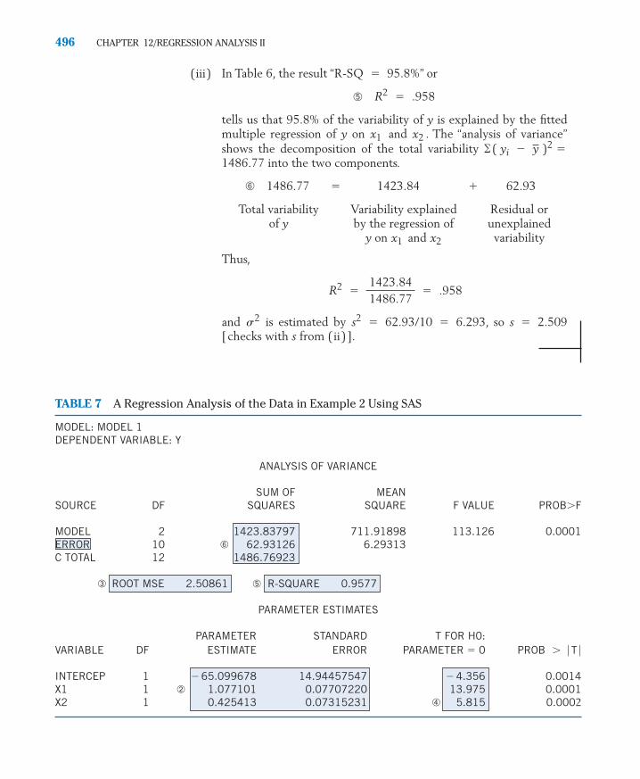
(iii) In Table 6, the result “R-SQ � 95.8%” or
➄
tells us that 95.8% of the variability of y is explained by the fittedmultiple regression of y on and . The “analysis of variance”shows the decomposition of the total variability �1486.77 into the two components.
➅ 1486.77 � 1423.84 � 62.93
Total variability Variability explained Residual orof y by the regression of unexplained
y on and variability
Thus,
and is estimated by � 62.93/10 � 6.293, so s � 2.509[checks with s from (ii)].
s2�
2
R2 �1423.841486.77
� .958
x2x1
( yi � y )2 �
x2x1
R2 � .958
496 CHAPTER 12/REGRESSION ANALYSIS II
TABLE 7 A Regression Analysis of the Data in Example 2 Using SAS
MODEL: MODEL 1DEPENDENT VARIABLE: Y
ANALYSIS OF VARIANCE
SUM OF MEANSOURCE DF SQUARES SQUARE F VALUE PROBF
MODEL 2 1423.83797 711.91898 113.126 0.0001ERROR 10 ➅ 62.93126 6.29313C TOTAL 12 1486.76923
➂ ROOT MSE 2.50861 ➄ R-SQUARE 0.9577
PARAMETER ESTIMATES
PARAMETER STANDARD T FOR H0:VARIABLE DF ESTIMATE ERROR PARAMETER � 0 PROB
INTERCEP 1 � 65.099678 14.94457547 � 4.356 0.0014X1 1 ➁ 1.077101 0.07707220 13.975 0.0001X2 1 0.425413 0.07315231 ➃ 5.815 0.0002
� T �
c12.qxd 10/15/09 11:18 AM Page 496

The square of the multiple correlation coefficient gives the proportionof variability in y explained by the fitted multiple regression.
The output from the SAS package is given in Table 7. The quantitiesneeded in our analysis have been labeled with the same circled numbers as inthe MINITAB output.
Example 3 Computer-Aided Regression Analysis—Two PredictorsThe times for 81 students to complete a rowing test both before and after com-pleting a one-semester conditioning course are given in Table D.5 in the DataBank. It may be that not only the pretest rowing time but also gender would beuseful for predicting the posttest rowing time. Perform a regression analysis.
SOLUTION We use MINITAB to obtain the output
Regression Analysis: Post row versus Pre row, Gender
The regression equation isPost row � 97.3 � 0.726 Pre row � 32.1 Gender
Predictor Coef SE Coef T PConstant 97.33 31.68 3.07 0.003Pre row 0.72573 0.05487 13.23 0.000Gender 32.083 9.756 3.29 0.002
S � 31.8137 R-Sq � 85.7% R-Sq(adj) � 85.3%
Analysis of Variance
Source DF SS MS F PRegression 2 471547 235774 232.95 0.000Residual Error 78 78945 1012Total 80 550492
Which variables should be used to predict posttest rowing time? Readingfrom the column of P–values for the individual coefficients, the largest is only.003. The constant term and the coefficients of pretest rowing time and genderare significantly different from 0.All three terms are needed in the model.
The plot of residuals versus fit in Figure 3 on page 498 reveals a constantwidth band so there is no evidence against the assumption of constant vari-ance. The one large negative residual is case 17 and the two large positiveresiduals are cases 29 and 70.
POLYNOMIAL REGRESSION
A scatter diagram may exhibit a relationship on a curve for which a suitable lin-earizing transformation cannot be constructed. Another method of handlingsuch a nonlinear relation is to include terms with higher powers of x in themodel Y � � � e. In this instance, by including the second powerof x, we obtain the model
�1 x�0
R2
3. MULTIPLE LINEAR REGRESSION 497
c12.qxd 10/15/09 11:18 AM Page 497

i � 1, . . . , n
which states that aside from the error components , the response y is aquadratic function (or a second-degree polynomial ) of the independent vari-able x. Such a model is called a polynomial regression model of y with x, andthe highest power of x that occurs in the model is called the degree or theorder of the polynomial regression. It is interesting to note that the analysisof a polynomial regression model does not require any special techniquesother than those used in multiple regression analysis. By identifying x and as the two variables and , respectively, this second-degree polynomialmodel reduces to the form of a multiple regression model:
i � 1, . . . , n
where and In fact, both these types of models and manymore types are special cases of a class called general linear models [1, 2].
Before we talk about the general linear model, let’s look at an examplewhich analyzes a second-degree polynomial model.
Example 4 Fitting a Quadratic Relation of a Human Development Index toInternet UsageRefer to Chapter 11, Example 9, concerning the development of a countrymeasured by the Human Development Index (HDI) and the predictor variableInternet usage per 100 persons. Although we randomly selected only fifteencountries, of the 152 countries, below the twenty-five most developed there isstill an indication that the relation is increasing less rapidly for high Internet us-age. Fit a quadratic and test whether or not squared term is required.
SOLUTION We fit the quadratic model usingMINITAB and obtain the output.
Yi � �0 � �1 xi � �2 xi2 � ei
xi 2 � x2i .xi 1 � x i
Yi � �0 � �1xi1 � �2 xi2 � ei
x2x1
x 2
ei
Yi � �0 � �1xi � �2 x 2
i � e i
498 CHAPTER 12/REGRESSION ANALYSIS II
100
50
0
�50
�100
500 600 700 800 900
Res
idua
l
Fit
Figure 3 Residuals of posttest row times versus fits.
c12.qxd 10/15/09 11:18 AM Page 498

The regression equation isHDI � 0.452 � 0.0356 Internet � 0.000789 Internet Sq
Predictor Coef SE Coef T PConstant 0.45213 0.02315 19.53 0.000Internet 0.035648 0.005557 6.41 0.000Internet Sq �0.00078930.0002322 -3.40 0.005
S � 0.0507320 R-Sq � 92.6%
Analysis of Variance
Source DF SS MS F PRegression 2 0.38684 0.19342 75.15 0.000Residual Error 12 0.03088 0.00257Total 14 0.41772
According to the output, the estimated coefficient of is = �.0007893 and the t test for testing : = 0 versus : 0 has P� value
P [T < �3.4] � P [T > 3.4] = .005
as indicated under P in the MINITAB output. This gives strong evidence that aquadratic term is needed. Note that the proportion of variation in HDI explainedby Internet usage has increased to .926 as indicated in the output R-Sq = 92.6%.
The data and fitted curve, shown in Figure 4, illustrate the bend in thestraight line relation at the few higher values of Internet usage. The quadraticfit is still not ideal because it starts to turn down over the range of the experi-ment, whereas the underlying relation is likely to always increase. This remindsus that there is no “true model,” but proposed models are only approximations.
��2H1�2H0
�2x 2
3. MULTIPLE LINEAR REGRESSION 499
Figure 4 Quadratic Fit to HDI by Internet Usage
0 5 10 15 20 25
HD
I
Internet/100
0.9
0.8
0.7
0.6
0.5
0.4
c12.qxd 10/15/09 11:18 AM Page 499

GENERAL LINEAR MODEL
By virtue of its wide applicability, the multiple linear regression model plays aprominent role in the portfolio of a statistician. Although a complete analysiscannot be given here, the general structure of a multiple regression model meritsfurther attention. We have already mentioned that most least squares analyses ofmultiple linear regression models are carried out with the aid of a computer.All the programs for implementing the analysis require the investigator to pro-vide the values of the response and the p input variables , . . . , for eachrun i � 1, 2, . . . , n. In writing 1 � , where 1 is the known value of an extra “dummy” input variable corresponding to , the model is�0
�0
x i px i 1yi
500 CHAPTER 12/REGRESSION ANALYSIS II
Input variables
� 1 � �0 � xi1 �1 � xi2 �2 � � � � � xip �p �Observation
Yi
Error
ei
This is called a linear model because it is linear in the ‘s. That is, there are noterms such as or .
The basic quantities can be arranged in the form of these arrays, which aredenoted by boldface letters.
Observation Input variables
Only the arrays y and X are required to obtain the least squares estimates of b0 ,, . . . , that minimize
The input array X is called the design matrix.In the same vein, setting
e � �e1e2�
�
�
en
� and � � ��0�1�
�
�
�p
��n
i � 1 ( yi � b0 � x i1 b1 � ��� � x i p bp)2
�p�1
y � �y1y2�
�
�
yi�
�
�
yn
� X � �11�
�
�
1�
�
�
1
x11x21
�
�
�
xi1�
�
�
xn1
���
���
���
���
���
���
���
���
���
���
x1px2p
�
�
�
xip�
�
�
xnp
�b1
2�2�1
�i
c12.qxd 10/15/09 11:18 AM Page 500

we can write the model in the suggested form
DesignObservation matrix Parameter Error
y � X � � e
which forms the basis for a thorough but more advanced treatment of regression.
Exercises
3. MULTIPLE LINEAR REGRESSION 501
12.6 A student fit the regression model Y � �
� � e to data from the fifty statesand Washington, D.C., so n = 51.The response y= median income in thousands of dollars and thetwo predictor variables are = median monthlyhousing costs for home owners and = percent-age of persons below the poverty level in the lasttwelve months.The least squares estimates are
Predict the response for
(a)
(b)
(c)
12.7 Consider the multiple linear regression model
where � � 2, � � 1, � 3, andthe normal random variable e has standard de-viation 3. What is the mean of the response Ywhen � 3 and � � 2?
12.8 In Exercise 12.6, suppose that the residual sumof squares (SSE) is 167.7 and the SS due toregression is 2538.7.
(a) Estimate the error standard deviation s.State the degrees of freedom.
(b) Find and interpret the result.
12.9 Refer again to Exercise 12.6 and assume that theassumptions about the model prevail. The esti-mated standard errors of and are .00107,and .0977, respectively.(a) Determine a 95% confidence interval for
.
(b) Test � � .0140 versus �
.0140, with a � .05.�1H1�1H0
�2
�2�1 ,
R2
x2x1
�2�1�0
Y � �0 � �1 x1 � �2 x2 � e
x1 � 1400, x2 � 15
x1 � 1200, x2 � 15
x1 � 1200, x2 � 13
�0 � 38.413 �1 � .0166 �2 � 1.008
x2
x1
�2 x2�1 x1
�012.10 Consider the data on all of the wolves in Table
D.9 of the Data Bank concerning age (years)and canine length (mm).
(a) Obtain the least squares fit of the straightline regression model Y � � �e to predict canine length from age.
(b) Obtain the least squares fit of the multi-ple regression model Y � � �
� e to predict canine length usingage and body length .
(c) What is the predicted canine length for awolf of age 2.5 and body length 127?
(d) What proportion of the y variability isexplained by the fitted model in Part (b)?
(e) Obtain 95% confidence intervals for ,, and .
12.11 Consider the response variable miles per gallon onhighways and the two predictor variables engine volume (l) and size of battery (v).Using the government 2009 Fuel Economy Guide,and the data on hybrid-electric cars and SUVs,we obtain the regression analysis given in Table 8.
(a) Identify the least squares estimates and
(b) What model is suggested from this analysis?
(c) What is the proportion of y variabilityexplained by the regression on and ?
(d) Estimate .
12.12 Laptop computers are advertised every weekby several stores. From one Sunday paper inMarch 2009, the response variable hard disksize(GB) and the two predictor variables
read-only memory(GB) and screensize (in) were recorded. The output from a re-gression analysis is given in Table 9, page 502.
x2 �x1 �
� 2
x2x1
�2 .�1 ,�0 ,
x2 �
x1 �
�2�1
�0
x2x1
�2 x2
�1 x1�0
�1 x�0
c12.qxd 10/15/09 11:18 AM Page 501

502 CHAPTER 12/REGRESSION ANALYSIS II
TABLE 8 Computer Output of a Regression Analysis to Be Used for Exercise 12.11
Regression Analysis: y versus x1, x2
The Regression equation isy � 45.3 � 3.22 x1 � 0.0207 X2
Predictor Coef SE Coef T PConstant 45.299 2.345 19.32 0.000x1 �3.2243 0.4562 �7.07 0.000x2 �0.020661 0.008574 �2.41 0.026
S � 3.40356 R-SQ � 79.5%
Analysis of Variance
Source DF SS MS F PRegression 2 897.53 448.77 38.74 0.000Error 20 231.68 11.58Total 22 1129.22
TABLE 9 Computer Output of a Regression Analysis to Be Used for Exercise 12.12
Regression Analysis: y versus x1, x2
The regression equation isY � � 258 � 61.7 X1 � 20.7 X2
Predictor Coef SE Coef T PConstant �257.8 117.9 �2.19 0.048x1 61.71 13.03 4.74 0.000x2 20.716 7.204 2.88 0.013
S � 35.3371 R-Sq � 72.3%
Analysis of Variance
Source DF SS MS F PRegression 2 42361 21180 16.96 0.000Residual Error 13 16233 1249Total 15 58594
(a) How many laptops were included in theanalysis?
(b) Identify the least squares estimates and
(c) What model is suggested from thisanalysis?
(d) What is the proportion of y variabilityexplained by the regression on and
?x2
x1
�2 .�1
,
�0 ,
12.13 With reference to Exercise 12.11:
(a) Test � � 0 versus � � 0with a � .05.
(b) Test � � 0 versus � � 0with a � .05.
(c) Estimate the expected y value correspond-ing to � 3.2 and � 200.
(d) Construct a 90% confidence interval forthe intercept .�0
x2x1
�2H1�2H0
�1H1�1H0
c12.qxd 10/15/09 11:18 AM Page 502

4. RESIDUAL PLOTS TO CHECK THE ADEQUACY OF A STATISTICAL MODEL 503
12.14 With reference to Exercise 12.12:
(a) Test � � 0 versus � � 0with a � .05.
(b) Test � � 0 versus � � 0with a � .05.
�2H1�2H0
�1H1�1H0
(c) Estimate the expected y value correspond-ing to � 2.0 and � 16.5.
(d) Construct a 90% confidence interval forthe intercept .�0
x2x1
4. RESIDUAL PLOTS TO CHECK THE ADEQUACY OF A STATISTICAL MODEL
General Attitude Toward a Statistical Model
A regression analysis is not completed by fitting a model by least squares,providing confidence intervals, and testing various hypotheses. These stepstell only half the story: the statistical inferences that can be made when thepostulated model is adequate. In most studies, we cannot be sure that a par-ticular model is correct. Therefore, we should adopt the following strategy.
1. Tentatively entertain a model.
2. Obtain least squares estimates and compute the residuals.
3. Review the model by examining the residuals.
Step 3 often suggests methods of appropriately modifying the model. We thenreturn to step 1, where the modified model is entertained, and this iteration iscontinued until a model is obtained for which the data do not seem to contra-dict the assumptions made about the model.
Once a model is fitted by least squares, all the information on variation thatcannot be explained by the model is contained in the residuals
where yi is the observed value and denotes the corresponding value predictedby the fitted model. For example, in the case of a simple linear regressionmodel, .
Recall from our discussion of the straight line model in Chapter 11 that wehave made the assumptions of independence, constant variance, and a normaldistribution for the error components . The inference procedures are based onthese assumptions. When the model is correct, the residuals can be consideredas estimates of the errors that are distributed as N(0, s).
To determine the merits of the tentatively entertained model, we can exam-ine the residuals by plotting them in various ways. Then if we recognize anysystematic pattern formed by the plotted residuals, we would suspect that someassumptions regarding the model are invalid. There are many ways to plot theresiduals, depending on what aspect is to be examined. We mention a few ofthese here to illustrate the techniques. A more comprehensive discussion can befound in Chapter 3 of Draper and Smith [2].
ei
ei
y i � �0 � �1 xi
y i
e i � yi � y i i � 1, 2, . . . , n
c12.qxd 10/15/09 11:18 AM Page 503

HISTOGRAM OR DOT DIAGRAM OF RESIDUALS
To picture the overall behavior of the residuals, we can plot a histogram for a largenumber of observations or a dot diagram for fewer observations. For example, in adot diagram like the one in Figure 5a, the residuals seem to behave like a sample
504 CHAPTER 12/REGRESSION ANALYSIS II
(a)0
(b)0
Residuals e
Residuals e
Figure 5 Dot diagram of residuals.(a) Normal pattern. (b) One large residual.
from a normal population and there do not appear to be any “wild” observations.In contrast, Figure 5b illustrates a situation in which the distribution appears to bequite normal except for a single residual that lies far to the right of the others. Thecircumstances that produced the associated observation demand a close scrutiny.
PLOT OF RESIDUAL VERSUS PREDICTED VALUE
A plot of the residuals versus the predicted value often helps to detect the in-adequacies of an assumed relation or a violation of the assumption of constant er-ror variance. Figure 6 illustrates some typical phenomena. If the points form a hori-zontal band around zero, as in Figure 6a, then no abnormality is indicated. InFigure 6b, the width of the band increases noticeably with increasing values of This indicates that the error variance tends to increase with an increasinglevel of response. We would then suspect the validity of the assumption of constantvariance in the model. Figure 6c shows residuals that form a systematic pattern. In-stead of being randomly distributed around the axis, they tend first to increasesteadily and then decrease. This would lead us to suspect that the model is inade-quate and a squared term or some other nonlinear x term should be considered.
PLOT OF RESIDUAL VERSUS TIME ORDER
The most crucial assumption in a regression analysis is that the errors areindependent. Lack of independence frequently occurs in business and economicapplications, where the observations are collected in a time sequence with theintention of using regression techniques to predict future trends. In many otherexperiments, trials are conducted successively in time. In any event, a plot of the
ei
y
� 2
y .
y iei
c12.qxd 10/15/09 11:18 AM Page 504

residuals versus time order often detects a violation of the assumption of inde-pendence. For example, the plot in Figure 7 exhibits a systematic pattern in thata string of high values is followed by a string of low values. This indicates thatconsecutive residuals are (positively) correlated, and we would suspect a viola-tion of the independence assumption. Independence can also be checked byplotting the successive pairs where indicates the residual fromthe first y value observed, indicates the second, and so on. Independence issuggested if the scatter diagram is a patternless cluster, whereas points clusteredalong a line suggest a lack of independence between adjacent observations.
e2
e1( ei , ei � 1 ) ,
4. RESIDUAL PLOTS TO CHECK THE ADEQUACY OF A STATISTICAL MODEL 505
e
y
(a)
e
y
(b)
e
y
(c)
Figure 6 Plot of residual versus predicted value.(a) Constant spread. (b) Increasing spread.(c) Systematic curved pattern.
Figure 7 Plot of residual versus time order.
e
Time order
c12.qxd 10/15/09 11:18 AM Page 505

506 CHAPTER 12/REGRESSION ANALYSIS II
The MINITAB regression four-in-one graphics option created four residualplots, including the three in Figure 8 using the data and fit from Example 3.
100
50
0
�50
�1001 10 20 30 40 50 60 70 80
Res
idua
lObservation Order
24
18
12
6
0�80 �40 0 40 80
Freq
uenc
y
Residual
Residuals Versus the Order of the DataHistogram of the Residuals
100
50
0
�50
�100500 900800700600
Res
idua
l
Fitted Value
Residuals Versus the Fitted Values
Figure 8 Three residual plots for posttest rowing time using MINITAB.
It is important to remember that our confidence in statistical inferenceprocedures is related to the validity of the assumptions about them.A mechanically made inference may be misleading if some modelassumption is grossly violated. An examination of the residuals is animportant part of regression analysis, because it helps to detect any incon-sistency between the data and the postulated model.
If no serious violation of the assumption is exposed in the process ofexamining residuals, we consider the model adequate and proceed with the rele-vant inferences. Otherwise, we must search for a more appropriate model.
References
1. S. Chatterjee and A. Hadi, Regression Analysis by Example, 4th ed., JohnWiley & Sons: New York, 2006.
2. N. R. Draper and H. Smith, Applied Regression Analysis, 3rd ed., John Wiley& Sons: New York, 1998.
3. D. Montgomery, E. Peck and G. Vinning, Introduction to Linear RegressionAnalysis, 3rd. ed., John Wiley & Sons: New York, 2001.
c12.qxd 10/15/09 11:18 AM Page 506

KEY IDEAS AND FORMULAS 507
USING STATISTICS WISELY
1. Always, as a first step, plot the response variable versus the predictorvariable. If there is more than one predictor variable, make separate plotsfor each. Examine the plot to see if a linear or other relationship exists.
2. Do not routinely accept the regression analysis presented in computer out-put. Instead, criticize the model by inspecting the residuals for outliers andmoderate to severe lack of normality. A normal-scores plot is useful if thereare more than 20 or so residuals.That plot may suggest a transformation.
3. Plot the residuals versus predicted value to check the assumption of con-stant variance. Plot the residuals in time order if that is appropriate.A trendover time would cast doubt on the assumption of independent errors.
KEY IDEAS AND FORMULAS
When a scatter diagram shows relationship on a curve, it may be possible tochoose a transformation of one or both variables such that the transformed dataexhibit a linear relation. A simple linear regression analysis can then be per-formed on the transformed data.
Multiple regression analysis is a versatile technique of building a predictionmodel with several input variables. In addition to obtaining the least squares fit,we can construct confidence intervals and test hypotheses about the influenceof each input variable.
A polynomial regression model is a special case of multiple regressionwhere the powers x , , , and so on, of a single predictor x play the role ofthe individual predictors.
The highest power of x that occurs in the model is called the degree ororder of the regression model. A quadratic function, or second-degree polyno-mial, is commonly fit as an alternative to a straight line.
Both the polynomial regression model and the multiple regression with sev-eral predictors are special cases of general linear models.
The measure , called the square of the multiple correlation coefficient,represents the proportion of y variability that is explained by the fitted multipleregression model.
To safeguard against a misuse of regression analysis, we must scrutinize thedata for agreement with the model assumptions. An examination of the residu-als, especially by graphical plots, including a dot diagram or histogram, a plotversus predicted value, and a plot versus time order, is essential for detectingpossible violations of the assumptions and also identifying the appropriate mod-ifications of an initial model.
R2 �Regression SS
Total SS
R2
x 3x
2
c12.qxd 10/15/09 11:18 AM Page 507

TECHNOLOGY
Regression with two or more predictors and quadratic regression
MINITAB
Regression with two or more predictors
Begin with the values for the two predictor variables in C2 and C3 and theresponse variable y in C1.
Stat Q Regression Q Regression.Type C1 in Response. Type C2 and C3 in Predictors.Select Graphs. Click Four in one. Click OK.Click OK.
The graphics step produces four residual plots: including histogram, residualversus fit, and residual versus order.
Transforming data
We illustrate with the predictor variable x in C2 and transforming to log(x),where the logarithm is base 10 in C3.
Calc Q Calculator.Type C3 in Store results in variable and LOGT(C2) in Expression.Click OK.
Fitting a quadratic regression model
With the values of x in C1 and the y values in C2, you must select:
Stat Q Regression Q Fitted Line Plot.Enter C2 in Response ( Y) and enter C1 in Predictor ( X ).Under Type of Regression Model choose Quadratic. Click OK.
TI-84/-83 PLUS
Fitting a quadratic regression model
Enter the values of the predictor variable in L1 and those of the response vari-able in L2.
Select STAT, then CALC, and then 5: QuadReg (ax � b).With LinReg on the Home screen press Enter.
The calculator will give a, b, and c in the equation
y � � bx � cax2
508 CHAPTER 12/REGRESSION ANALYSIS II
c12.qxd 10/15/09 11:18 AM Page 508

5. REVIEW EXERCISES 509
Time x(days) No. Type 1 No. Type 2
17 137 586 .2331 278 479 .5845 331 167 1.9859 769 227 3.3973 976 75 13.01
y �No. Type 1
No. Type 2
5. REVIEW EXERCISES
12.15 An environmental scientist identified a pointsource for E. Coli at the edge of a stream. Shethen measured y = E. Coli, in colony formingunits per 100 ml water, at different distances, infeet, downstream from the point source. Sup-pose she obtains the following pairs of ( x , y).
x 100 150 250 250 400 650 1000 1600
y 21 20 24 17 18 10 11 9
(b) Determine if a linear relation is plausiblefor the transformed data y� � y.
(c) Fit a straight line regression to the trans-formed data.
12.18 Refer to the 2007 campus crime data in Chap-ter 11, Table 5. Obtaining the least squares fitto the response y = number of arson incidents,using the two predictor variables = robberyand = forceable rape, gives the results
(a) Predict the response for
(i) � 7 and � 5
(ii) � 15 and � 11(b) Estimate the error standard deviation s
and state the degrees of freedom.(c) What proportion of the y variability is
explained by the fitted regression?12.19 Refer to Exercise 12.18. The estimated stan-
dard errors of and were .1085 and .0451,respectively.(a) Obtain a 90% confidence interval for b1 .(b) Test � � .10 versus � .10
with a � .05.12.20 A second-degree polynomial
is fitted to a response y, and the followingpredicted values and residuals are obtained.�2 x
2y � �0 � �1 x �
��2H1�2H0
�2�1
x2x1
x2x1
SSE � 113.15SS due to regression � 245.40
�0 � � .3780 �1 � .3401 �2 � .1826
x2
x1
log10
(a) Transform the x values to x� � xand plot the scatter diagram of y versus x�.
(b) Fit a straight line regression to the trans-formed data.
(c) Obtain a 90% confidence interval for theslope of the regression line.
(d) Estimate the expected y value corre-sponding to x � 300 and give a 95%confidence interval.
*12.16 Obtain a linearizing transformation in each case.
(a)
(b)
12.17 A genetic experiment is undertaken to studythe competition between two types of femaleDrosophila melanogaster in cages with one malegenotype acting as a substrate. The independentvariable x is the time spent in cages, and the de-pendent variable y is the ratio of the numbersof type 1 to type 2 females. The following data(courtesy of C. Denniston) are recorded.
y � eaxb
y �1
(1 � aebx )2
log10
Residuals
4.01 .285.53 � .336.21 � .216.85 .248.17 � .978.34 .468.81 .799.62 � 1.02
10.05 1.3510.55 � 1.5510.77 .6310.77 1.7310.94 � 2.1410.98 1.9210.98 � 1.18
y
(a) Plot the scatter diagram of y versus x anddetermine if a linear model of relation isappropriate.
c12.qxd 10/15/09 11:18 AM Page 509

Do the assumptions appear to be violated?
12.21 The following predicted values and residuals areobtained in an experiment conducted to deter-mine the degree to which the yield of an impor-tant chemical in the manufacture of penicillin isdependent on sugar concentration (the timeorder of the experiments is given in parentheses).
(a) Plot the residuals against the predictedvalues and also against the time order.
(b) Do the basic assumptions appear to beviolated?
12.22 An experimenter obtains the following residualsafter fitting a quadratic expression in x.
Do the basic assumptions appear to be violated?
12.23 An interested student used the method ofleast squares to fit the straight line
x to gross national product, y,in real dollars. The results for 26 recent years,x � 1, 2, . . . , 26, appear below. Whichassumption(s) for a linear regression modelappear to be seriously violated by the data?(Note: Regression methods are usually notappropriate for this type of data.)
264.3 � 18.77y �
510 CHAPTER 12/REGRESSION ANALYSIS II
x � 1 x � 2 x � 3 x � 4 x � 5
� .1 1.3 � .1 0 � .20 � .2 � .3 .2 0
� .2 � .1 .1 � .1 � .2.6 � .3 .4 0 � .2
� .1 .1 � .1 � .2 � .3.1 � .1
The Following Exercises Require a Computer
12.24 Consider the data on male wolves in Table D.9of the Data Bank concerning age (years) andcanine length (mm).
(a) Obtain the least squares fit of caninelength to the predictor age.
(b) Obtain the least squares fit of caninelength to a quadratic function of the pre-dictor age. The MINITAB commands are
Data: DBT9.txtC2: 4 2 4 � � � 0C6: 28.7 27.0 27.2 � � � 24.5Dialog box:
Stat Q Regression Q Fitted line plotType C6 in Response.Type C2 in Predictor.Click Quadratic. Click OK.
Predicted Residual
2.2(9) � 13.1(6) � 22.5(13) 33.3(1) � 32.3(7) � 13.6(14) 52.6(8) 02.5(3) 03.0(12) 33.2(4) � 22.9(11) 23.3(2) � 52.7(10) 03.2(5) 1
Year y Residual
1 309.9 283.1 26.82 323.7 301.9 21.83 324.1 320.6 3.54 355.3 339.4 15.95 383.4 358.2 25.26 395.1 376.9 18.27 412.8 395.7 17.18 407 414.5 � 7.59 438 433.2 4.8
10 446.1 452.0 � 5.911 452.5 470.8 � 18.312 447.3 489.5 � 42.213 475.9 508.3 � 32.414 487.7 527.1 � 39.415 497.2 545.8 � 48.616 529.8 564.6 � 34.817 551 583.4 � 32.418 581.1 602.1 � 21.019 617.8 620.9 � 3.120 658.1 639.7 18.421 675.2 658.4 16.822 706.6 677.2 29.423 725.6 696.0 29.624 722.5 714.7 7.825 745.4 733.5 11.926 790.7 752.3 38.4
y
c12.qxd 10/15/09 11:18 AM Page 510

5. REVIEW EXERCISES 511
the meaning of the coefficients and
(b) Give 95% confidence intervals for and.
(c) Obtain R2 and interpret the result.
12.27 Refer to the data of speed x and stoppingdistance y given in Table 1. The MINITABcommands for fitting a straight line regressionto and x arey� � √y
�2
�1
�2 .�1
Data: C12T1.txt
C1: 20 20 30 30 30 40 40 50 50 60
C2: 16.3 26.7 39.2 63.5 51.3 98.4 65.7 104.1 155.6 217.2
Dialog box:
Calc Q Calculator
Type SQRT(C2) in the Expression box.
Type C3 in Store box. Click OK.
Stat Q Regression Q Regression
Type C3 in Response.
Type C1 in Predictors. Click OK.
(c) What proportion of the y variability is ex-plained by the quadratic regression model?
(d) Compare the estimated standard devia-tions, s, of the random error term in parts(a) and (b).
12.25 The resident population of the United Stateshas grown over the last 100 years from 1910to 2010 but the growth has not been linear.The response variable is y = population in mil-lions and, to simplify the calculations, the pre-dictor variable is x = year 2 1900.
x 10 20 30 40 50 60
y 92.2 106.0 123.2 132.2 151.3 179.3
x 70 80 90 100 110
y 203.3 226.5 248.7 281.4 310.2
(a) Fit a quadratic regression model Y � �� � e to these data.
(b) What proportion of the y variability is ex-plained by the quadratic regression model?
(c) Test : � 0 versus � 0 witha � .05.
12.26 Listed below are the price quotations for amidsize foreign used car along with their ageand odometer mileage.
�1H1�1H0
�2 x2�1
x�0
Mileage Price yAge (thousand (thousand
(years) miles) miles)
1 14 17.92 44 13.92 20 14.94 36 14.04 66 9.85 59 9.97 100 6.67 95 6.78 38 7.0
x1
x2
Perform a multiple regression analysis of thesedata. In particular
(a) Determine the equation for predictingthe price from age and mileage. Interpret
(a) Obtain the computer output and identifythe equation of the fitted line and thevalue of (see Example 1).
(b) Give a 95% confidence interval for the slope.
(c) Obtain a 95% confidence interval for theexpected y� value at x � 45.
12.28 A forester seeking information on basic treedimensions obtains the following measure-ments of the diameters 4.5 feet above theground and the heights of 12 sugar mapletrees (courtesy of A. Ek). The forester wishesto determine if the diameter measurementscan be used to predict the tree height.(a) Plot the scatter diagram and determine if
a straight line relation is appropriate.
(b) Determine an appropriate linearizing trans-formation. In particular, try x� � log x ,y� � log y .
(c) Fit a straight-line regression to the trans-formed data.
r
2
c12.qxd 10/15/09 11:18 AM Page 511
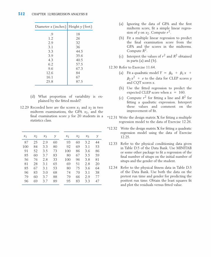
512 CHAPTER 12/REGRESSION ANALYSIS II
(a) Ignoring the data of GPA and the firstmidterm score, fit a simple linear regres-sion of y on . Compute .
(b) Fit a multiple linear regression to predictthe final examination score from theGPA and the scores in the midterms.Compute .
(c) Interpret the values of and obtainedin parts (a) and (b).
12.30 Refer to Exercise 11.64.
(a) Fit a quadratic model Y � � �
� e to the data for CLEP scores yand CQT scores x.
(b) Use the fitted regression to predict theexpected CLEP score when x � 160.
(c) Compute for fitting a line and forfitting a quadratic expression. Interpretthese values and comment on theimprovement of fit.
*12.31 Write the design matrix X for fitting a multipleregression model to the data of Exercise 12.26.
*12.32 Write the design matrix X for fitting a quadraticregression model using the data of Exercise12.25.
12.33 Refer to the physical conditioning data givenin Table D.5 of the Data Bank. Use MINITABor some other package to fit a regression of thefinal number of situps on the initial number ofsitups and the gender of the student.
12.34 Refer to the physical fitness data in Table D.5of the Data Bank. Use both the data on thepretest run time and gender for predicting theposttest run time. Obtain the least squares fitand plot the residuals versus fitted value.
R2r
2
�2 x
2�1 x�0
R2r
2R2
r
2x2
y
87 25 2.9 60100 84 3.3 8091 52 3.5 7385 60 3.7 8356 76 2.8 3381 28 3.1 6585 67 3.1 5396 83 3.0 6879 60 3.7 8896 69 3.7 89
x3x2x1 y
93 60 3.2 4492 69 3.1 53
100 86 3.6 8680 67 3.5 59
100 96 3.8 8169 51 2.8 2080 75 3.6 6474 70 3.1 3879 66 2.9 7795 83 3.3 47
x3x2x1
(d) What proportion of variability is ex-plained by the fitted model?
12.29 Recorded here are the scores and in twomidterm examinations, the GPA , and thefinal examination score y for 20 students in astatistics class.
x3
x2x1
Diameter x ( inches) Height y (feet)
.9 181.2 262.9 323.1 363.3 44.53.9 35.64.3 40.56.2 57.59.6 67.3
12.6 8416.1 6725.8 87.5
c12.qxd 10/15/09 11:18 AM Page 512

13
Analysis ofCategorical Data
1. Introduction2. Pearson’s Test for Goodness of Fit3. Contingency Table with One Margin Fixed
(Test of Homogeneity)4. Contingency Table with Neither Margin Fixed
(Test of Independence)5. Review Exercises
�2
c13.qxd 10/15/09 11:20 AM Page 513

Are Firm Mattresses Really Best?Although it is commonly believed that firm mattresses can help persons withlow-back pain, experimental evidence was lacking. Medical researchers1 designeda carefully designed experiment. Of the patients admitted to the study, 158 wererandomly selected to sleep on a new firm mattress and the others were givennew medium-firm mattresses. The patients were not told about the firmness oftheir new mattresses although most perceived the correct firmness. The personswho installed the new beds and the research assistants who collected the datafrom patients were also kept unaware of the firmness of the mattresses.
This design includes meritable features: (1) the random assignment of treat-ments (mattress firmness) and (2) the double blind feature where patient andresearcher are not told which treatment has been assigned.
The patients were asked to report whether or not they had low-back painupon arising during the 90-day follow-up period.
1Source: F. Kovacs et al., "Effect of firmness of mattress on chronic non-specific low-back pain: random-ized, double-blind, controlled, multicentre trial," The Lancet 362 (November 15, 2003), pp. 1599–1604.
Courtesy of Roberta Johnson.
Low Back Pain
Firmness No Yes Total
Firm 36 122 158Medium firm 55 95 150
The proportion with no low-back pain upon arising is .228 � 36/158 forthose who slept on firm mattresses and the proportion is .367 � 55/150 forthose who slept on medium-firm mattresses. These data provide convincing evi-dence that medium-firm mattresses reduce low-back pain upon arising. TheP–value for the test of equality of the proportions, of persons in each populationwho would answer No, versus a two-sided alternative is .008. In less than 1 in 100times would chance variation give an observed difference this large or larger.
c13.qxd 10/15/09 11:20 AM Page 514
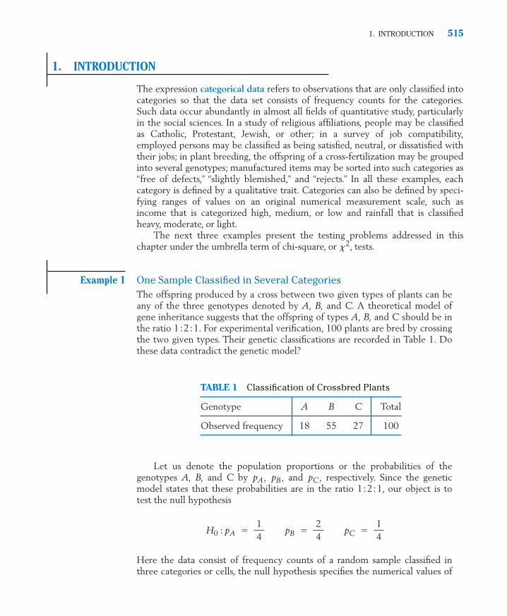
1. INTRODUCTION
The expression categorical data refers to observations that are only classified intocategories so that the data set consists of frequency counts for the categories.Such data occur abundantly in almost all fields of quantitative study, particularlyin the social sciences. In a study of religious affiliations, people may be classifiedas Catholic, Protestant, Jewish, or other; in a survey of job compatibility,employed persons may be classified as being satisfied, neutral, or dissatisfied withtheir jobs; in plant breeding, the offspring of a cross-fertilization may be groupedinto several genotypes; manufactured items may be sorted into such categories as“free of defects,” “slightly blemished,” and “rejects.” In all these examples, eachcategory is defined by a qualitative trait. Categories can also be defined by speci-fying ranges of values on an original numerical measurement scale, such asincome that is categorized high, medium, or low and rainfall that is classifiedheavy, moderate, or light.
The next three examples present the testing problems addressed in thischapter under the umbrella term of chi-square, or , tests.
Example 1 One Sample Classified in Several CategoriesThe offspring produced by a cross between two given types of plants can beany of the three genotypes denoted by A, B, and C. A theoretical model ofgene inheritance suggests that the offspring of types A, B, and C should be inthe ratio 1�2�1. For experimental verification, 100 plants are bred by crossingthe two given types. Their genetic classifications are recorded in Table 1. Dothese data contradict the genetic model?
Let us denote the population proportions or the probabilities of thegenotypes A, B, and C by , , and , respectively. Since the geneticmodel states that these probabilities are in the ratio 1�2�1, our object is totest the null hypothesis
Here the data consist of frequency counts of a random sample classified inthree categories or cells, the null hypothesis specifies the numerical values of
H0 �pA �14 pB �
24 pC �
14
pCpBpA
�2
1. INTRODUCTION 515
TABLE 1 Classification of Crossbred Plants
Genotype A B C Total
Observed frequency 18 55 27 100
c13.qxd 10/15/09 11:20 AM Page 515

the cell probabilities, and we wish to examine if the observed frequenciescontradict the null hypothesis.
Example 2 Independent Samples Classified in Several CategoriesTo compare the effectiveness of two diets A and B, 150 infants were includedin a study. Diet A was given to 80 randomly selected infants and diet B to theother 70 infants. At a later time, the health of each infant was observed andclassified into one of the three categories “excellent,” “average,” and “poor.”From the frequency counts recorded in Table 2, we wish to test the nullhypothesis that there is no difference between the quality of the two diets.
The two rows of Table 2 have resulted from independent samples. Fora descriptive summary of these data, it is proper to compute the relativefrequencies for each row. These are given in Table 2(a).
The (unknown) population proportions or probabilities are entered inTable 2( b). They allow us to describe the null hypothesis more clearly. Thenull hypothesis of “no difference” is equivalent to the statement that, for eachresponse category, the probability is the same for diet A and diet B. Conse-quently, we formulate
H0 � pA1 � pB1 pA2 � pB2 pA3 � pB3
516 CHAPTER 13/ANALYSIS OF CATEGORICAL DATA
TABLE 2 (a) Relative Frequencies (from Table 2)
Excellent Average Poor Total
Diet A .46 .30 .24 1Diet B .24 .47 .29 1
TABLE 2 Health under Two Different Diets
SampleExcellent Average Poor Size
Diet A 37 24 19 80Diet B 17 33 20 70
Total 54 57 39 150
c13.qxd 10/15/09 11:20 AM Page 516

Note that although specifies a structure for the cell probabilities, it doesnot give the numerical value of the common probability in each column.
Example 3 One Sample Simultaneously Classified According to Two CharacteristicsImproperly disclosed personal information has become a major source lead-ing to credit fraud. In a survey conducted to help investigate the pervasive-ness of the problem, 395 respondents reported receiving notification thattheir personal data had been compromised. Each of these cases were thenclassified according to type of institution sending the notification and alsowhether or not harm was caused to the person’s credit. Harm to credit pri-marily includes instances of charging merchandise or taking money frombank accounts. Attention was restricted to institutions categorized as
Government (federal, state and local)Financial (bank, investment organization, credit firm, or insurance)Other Commercial (Internet, retail, or communications company).
The cell frequencies for the two-way classification are given in Table 3.Do the data indicate that the pattern of cases of harmed credit, caused by
the release of personal data, differs among the three types of organizations?
Unlike Example 2, here we have a single random sample, but each sampledindividual elicits two types of response: source of notification and whether or notharm was done to credit. In the present context, the null hypothesis of “no differ-ence’’ amounts to saying the outcome on credit and type of institution givingnotification are independent. In other words, whether or not harm was done isunrelated to, or independent of, the type of institution that improperly disclosedpersonal information. A formal specification of this null hypothesis, in terms ofthe cell probabilities, is deferred until Section 4.
2
H0
TABLE 3 Type of Organization and Fraudulent Use of Personal Information
Government Financial Other Commercial Total
Harm 30 24 21 75No Harm 182 104 34 320
Total 212 128 55 395
TABLE 2(b) Population Proportions or Probabilities
Excellent Average Poor Total
Diet A 1Diet B 1pB3pB2pB1
pA3pA2pA1
1. INTRODUCTION 517
The resulting proportions are close to those reported in a 2006 survey by Harris Interactive.2
c13.qxd 10/15/09 11:20 AM Page 517

Frequency count data that arise from a classification of the sample observa-tions according to two or more characteristics are called cross-tabulated data ora contingency table. If only two characteristics are observed and the contingencytable has r rows and c columns, it is designated as an r � c table. Thus, Tables 2and 3 are both 2 � 3 contingency tables.
Although Tables 2 and 3 have the same appearance, there is a fundamentaldifference in regard to the method of sampling. The row totals 80 and 70 inTable 2 are the predetermined sample sizes; these are not outcomes of randomsampling, as are the column totals. By contrast, both sets of marginal totals inTable 3 are outcomes of random sampling—none were fixed beforehand. Todraw the distinction, one often refers to Table 2 as a 2 � 3 contingency tablewith fixed row totals. In Sections 3 and 4, we will see that the formulation ofthe null hypothesis is different for the two situations.
2. PEARSON’S TEST FOR GOODNESS OF FIT
We first consider the type of problem illustrated in Example 1, where the dataconsist of frequency counts observed from a random sample and the nullhypothesis specifies the unknown cell probabilities. Our primary goal is to test ifthe model given by the null hypothesis fits the data, and this is appropriatelycalled testing for goodness of fit.
For general discussion, suppose a random sample of size n is classified into kcategories or cells labeled 1, 2, . . . , k and let , , . . . , denote therespective cell frequencies. If we denote the cell probabilities by , , . . . , ,a null hypothesis that completely specifies the cell probabilities is of the form
where are given numerical values that satisfy
From Chapter 5 recall that if the probability of an event is p, then theexpected number of occurrences of the event in n trials is np. Therefore, oncethe cell probabilities are specified, the expected cell frequencies can be readilycomputed by multiplying these probabilities by the sample size n. A goodness offit test attempts to determine if a conspicuous discrepancy exists between theobserved cell frequencies and those expected under . (See Table 4.)
A useful measure for the overall discrepancy between the observed andexpected frequencies is given by the chi-square or statistic.� 2
H0
� pk 0 � 1.p10 � � � �p10
, . . . , pk 0
H0 � p1 � p10 , . . . , pk � pk 0
pkp2p1
nkn2n1
�2
518 CHAPTER 13/ANALYSIS OF CATEGORICAL DATA
TABLE 4 The Basis of a Goodness of Fit Test
Cells 1 2 � � � k Total
Observed frequency O � � � nProbability under � � � 1Expected frequency E
under n n � � � n npk 0p20p10H0
pk 0p20p10H0
nkn2n1
c13.qxd 10/15/09 11:20 AM Page 518

where O and E symbolize an observed frequency and the correspondingexpected frequency. The discrepancy in each cell is measured by the squareddifference between the observed and the expected frequencies divided by theexpected frequency. The measure is the sum of these quantities for all cells.
The statistic was originally proposed by Karl Pearson (1857–1936), whofound the distribution for large n to be approximately a distribution with d.f. � k � 1. Due to this distribution, the statistic is denoted by and calledPearson’s statistic for goodness of fit. Because a large value of the overalldiscrepancy indicates a disagreement between the data and the null hypothesis,the upper tail of the distribution constitutes the rejection region.
It should be remembered that Pearson’s test is an approximate test thatis valid only for large samples. As a rule of thumb, n should be large enough sothat the expected frequency of each cell is at least 5.
Example 4 Goodness of Fit for a Genetic ModelReferring to Example 1, test the goodness of fit of the genetic model to thedata in Table 1. Take � � .05.
SOLUTION Following the structure of Table 4, the computations for the statistic areexhibited in Table 5 where the last line gives the calculation
�2
�2
�2
�2
� 2�2
�2 �2
�2
�2 � �k
i � 1 ( ni � n pi0
)2
n pi 0� �
cells (O � E )2
E
Pearson’s Test for Goodness of Fit ( Based on Large n )
Null hypothesis
Test statistic
Rejection region
where is the upper � point of the distribution with
d.f. � k � 1 � (Number of cells) � 1
�2 ��2
�2 � ��2
�2 � �k
i � 1 ( ni � n pi0 )2
n pi 0� �
cells ( O � E )2
E
H0 � p1 � p10 , . . . , pk � pk 0
�2
2. PEARSON’S �2 TEST FOR GOODNESS OF FIT 519
� 1.96
�cells
( O � E )2
E�
( 18 � 25)2
25�
( 55 � 50 )2
50�
( 27 � 25 )2
25
.50� � .16 � 2.62
c13.qxd 10/15/09 11:20 AM Page 519

We use the statistic with rejection region R� � 5.99 since 5.99 with d.f. � 2 (Appendix B, Table 5). Because the observed � 2.62is smaller than this value, the null hypothesis is not rejected at � � .05. Weconclude that the data in Table 1 do not contradict the genetic model.
The statistic measures the overall discrepancy between the observed fre-quencies and those expected under a given null hypothesis. Example 4 demon-strates its application when the frequency counts arise from a single randomsample and the categories refer to only one characteristic—namely, the geno-type of the offspring. Basically, the same principle extends to testing hypotheseswith more complex types of categorical data such as the contingency tablesillustrated in Examples 2 and 3. In preparation for these developments, we statetwo fundamental properties of the statistic:�2
�2
�2 �.05
2 ��2 �2
520 CHAPTER 13/ANALYSIS OF CATEGORICAL DATA
TABLE 5 The Goodness of Fit Test for the Data in Table 1
Cell A B C Total
Observed frequency O 18 55 27 100Probability under .25 .50 .25 1.0Expected frequency E 25 50 25 100
1.96 .50 .16 2.62 � �2
d.f. � 2( O � E )2
E
H0
�2
Properties of Pearson’s Statistic
1. Additivity: If statistics are computed from independent samples,then their sum is also a statistic whose d.f. equals the sum of thed.f.’s of the components.
2. Loss of d.f. due to estimation of parameters: If does not com-pletely specify the cell probabilities, then some parameters have to beestimated in order to obtain the expected cell frequencies. In thatcase, the d.f. of is reduced by the number of parameters estimated.
d.f. of � ( No. of cells) � 1 � ( No. of parameters estimated )�2
�2
H0
�2 �2
�2
c13.qxd 10/15/09 11:20 AM Page 520

Exercises
2. PEARSON’S �2 TEST FOR GOODNESS OF FIT 521
Blood type O A B AB Total
Frequency 40 44 10 6 100
Color White Stainless Black Total
Frequency 63 56 31 150
13.1 Given below are the frequencies observedfrom 320 tosses of a die. Do these data castdoubt on the fairness of the die?
13.2 Recorded here is the frequency distributionof the blood types of 100 persons who havevolunteered to donate blood at a plasmacenter.
Test the goodness of fit of the model, whichassumes that the four blood types are equallylikely in the population of plasma donors. Use� � .05.
13.3 Referring to the data in Exercise 13.2, test thenull hypothesis that the probability of theblood types O, A, B, and AB is in the ratios4�4�1�1. Use � � .05.
13.4 A market researcher wishes to assess consumers’preference among three different colors availableon name-brand dishwashers. The following fre-quencies were observed from a random sampleof 150 recent sales.
Test the null hypothesis, at � � .05, that allthree colors are equally popular.
13.5 A shipment of assorted nuts is labeled ashaving 45% walnuts, 20% hazelnuts, 20%almonds, and 15% pistachios. By randomlypicking several scoops of nuts from this ship-ment, an inspector finds the counts shown atthe top of next column.Could these findings be a strong basis for an accusation of mislabeling? Test at � � .025.
13.6 Cross-fertilizing a pure strain of red flowerswith a pure strain of white flowers producespink hybrids that have one gene of each type.Crossing these hybrids can lead to any oneof four possible gene pairs. Under Mendel’s the-ory, these four are equally likely, so
P (white) � P (pink) � P (red) �
An experiment carried out by Correns, one ofMendel’s followers, resulted in the frequencies141, 291, and 132 for the white, pink, and redflowers, respectively. (Source: W. Johannsen,1909, Elements of the Precise Theory of Heredity,G. Fischer, Jena.)
Do these observations appear to contradictthe probabilities suggested by Mendel’s theory?
13.7 According to the records of the National SafetyCouncil, accidental deaths in the United Statesduring 2005 had the following distribution ac-cording to the principal types of accidents.
14
12
14
Face No. 1 2 3 4 5 6 Total
Frequency 39 63 56 67 57 38 320
Motor Vehicle Poison Falls Choking Drowning Other
40.5% 18.5% 15.7% 4.1% 3.2% 18.0%
Counts
Walnuts 95Hazelnuts 70Almonds 33Pistachios 42
Total 240
Motor Vehicle Poison Falls Choking Drowning Other Total
356 207 125 33 26 161 908
In a particular geographical region, the acciden-tal deaths, classified according to the principaltypes of accidents, yielded the followingfrequency distribution.
Do these data show a significantly different distri-bution of accidental deaths as compared to thatfor the entire United States? Test at � � .05.
c13.qxd 10/15/09 11:20 AM Page 521

3. CONTINGENCY TABLE WITH ONE MARGIN FIXED (TEST OF HOMOGENEITY)
From each population, we draw a random sample of a predetermined samplesize and classify each response in categories. These data form a two-way contin-gency table where one classification refers to the populations and the other tothe response under study. Our objective is to test whether the populations arealike, or homogeneous, with respect to cell probabilities. To do so, we will deter-mine if the observed proportions in each response category are nearly the samefor all populations.
Let us pursue our development of the test of homogenity with the dataof Table 2.
Example 5 Developing a Test to Compare Two DietsReferring to Example 2, test the null hypothesis that there is no differencebetween the quality of the two diets.
�2
�2
13.8 The following table, based on government data,shows the frequency distribution of births byday of the week for all registered births in theUnited States in a recent year. Test the nullhypothesis, at � � .01, that all seven days ofthe week are equally likely for childbirth.
522 CHAPTER 13/ANALYSIS OF CATEGORICAL DATA
Under the model of Bernoulli trials for the sexof rabbits, the probability distribution of thenumber of males per litter should be binomialwith 3 trials and p � probability of a male birth.From these data, the parameter p is estimated as
(a) Using the binomial table for three trials anddetermine the cell probabilities.
(b) Perform the test for goodness of fit.(In determining the d.f., note that one pa-rameter has been estimated from the data.)
*13.10 An alternative expression for Pearson’s . Byexpanding the square on the right-hand side of
show that the statistic can also be expressed as
�2 � �cells
O2
E� n
�2 � �cells
ni
2
npi 0� n that is,
�2
�2 � �cells
( ni � npi 0
)2
npi 0
�2
�2
p � .4,
�97240
� .4
p �Total number of males in 80 littersTotal number of rabbits in 80 litters
Number of males in litter 0 1 2 3 Total
Number of litters 19 32 22 7 80
Number of Births (in 10,000) by Day of the Week, United States
Number of births
Mon. 62.81Tues. 69.66Wed. 70.11Thurs. 69.91Fri. 68.39Sat. 45.47Sun. 40.21
All Days 426.56
Source: J. Martin et al, “Births: Final Data for2006,” National Vital Statistics Reports 57, No. 7(2009),Table 17.
13.9 Observations of 80 litters, each containing3 rabbits, reveal the following frequency distri-bution of the number of male rabbits per litter.
c13.qxd 10/15/09 11:20 AM Page 522
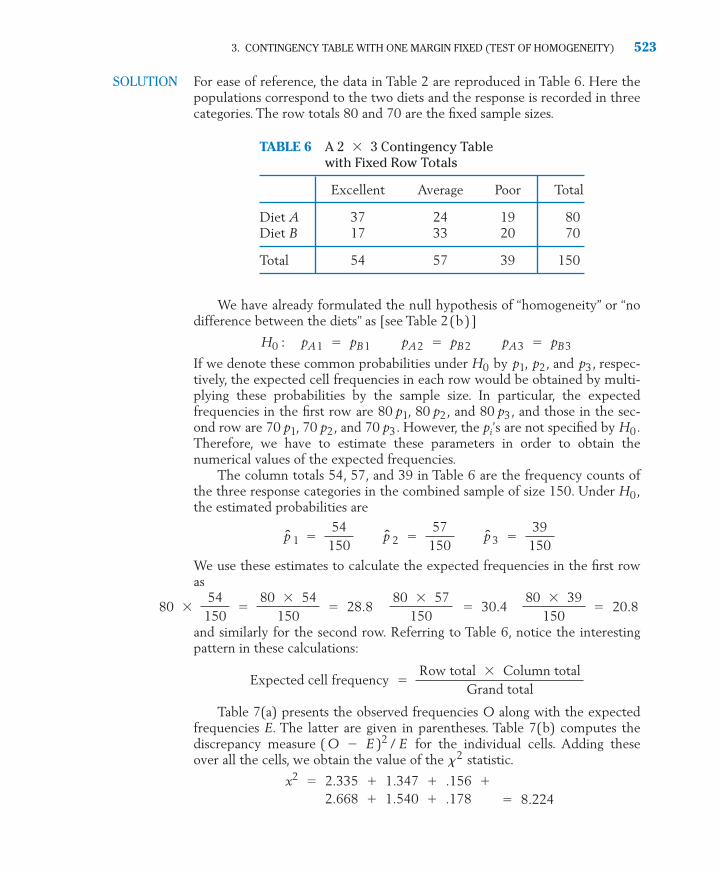
3. CONTINGENCY TABLE WITH ONE MARGIN FIXED (TEST OF HOMOGENEITY) 523
SOLUTION For ease of reference, the data in Table 2 are reproduced in Table 6. Here thepopulations correspond to the two diets and the response is recorded in threecategories. The row totals 80 and 70 are the fixed sample sizes.
We have already formulated the null hypothesis of “homogeneity” or “nodifference between the diets” as [see Table 2(b)]
If we denote these common probabilities under by , , and , respec-tively, the expected cell frequencies in each row would be obtained by multi-plying these probabilities by the sample size. In particular, the expectedfrequencies in the first row are 80 , 80 , and 80 , and those in the sec-ond row are 70 , 70 , and 70 . However, the pi’s are not specified by .Therefore, we have to estimate these parameters in order to obtain thenumerical values of the expected frequencies.
The column totals 54, 57, and 39 in Table 6 are the frequency counts ofthe three response categories in the combined sample of size 150. Under ,the estimated probabilities are
We use these estimates to calculate the expected frequencies in the first rowas
and similarly for the second row. Referring to Table 6, notice the interestingpattern in these calculations:
Table 7(a) presents the observed frequencies O along with the expectedfrequencies E. The latter are given in parentheses. Table 7(b) computes thediscrepancy measure for the individual cells. Adding theseover all the cells, we obtain the value of the statistic.�2
( O � E )2 / E
Expected cell frequency �Row total � Column total
Grand total
80 �54
150�
80 � 54150
� 28.8 80 � 57150
� 30.4 80 � 39150
� 20.8
p 1 �54
150 p 2 �
57150
p 3 �39
150
H0
H0p3p2p1
p3p2p1
p3p2p1H0
H0 � pA 1 � pB 1 pA 2 � pB 2 pA 3 � pB 3
TABLE 6 A 2 � 3 Contingency Table with Fixed Row Totals
Excellent Average Poor Total
Diet A 37 24 19 80Diet B 17 33 20 70
Total 54 57 39 150
2.668 � 1.540 � .178x2 � 2.335 � 1.347 � .156 �
� 8.224
c13.qxd 10/15/09 11:20 AM Page 523

524 CHAPTER 13/ANALYSIS OF CATEGORICAL DATA
In order to determine the degrees of freedom, we employ the propertiesof the statistic stated in Section 2. Our statistic has been computedfrom two independent samples; each contributes 3 � 1 � 2 d.f. becausethere are three categories. The added d.f. � 2 � 2 � 4 must now be reducedby the number of parameters we have estimated. Since , , and satisfythe relation there are really two undetermined para-meters among them. Therefore, our statistic has d.f. � 4 � 2 � 2.
With d.f. � 2, the tabulated upper 5% point of is 5.99 (Appendix B,Table 5). Since the observed � 8.224 is larger, the null hypothesis is rejected at � � .05. It would also be rejected at � � .025. Therefore, a signifi-cant difference between the quality of the two diets is indicated by the data.
Having obtained a significant , we should now examine Tables 7(a)and 7(b) and try to locate the source of the significance. We find that largecontributions to come from the “excellent” category, where the relativefrequency is 37/80, or 46%, for diet A and 17/ 70, or 24%, for diet B. Thesedata indicate that A is superior.
Motivated by Example 5, we are now ready to describe the test proce-dure for an contingency table that has independent samples from r pop-ulations that are classified in c response categories. As we have seen before, theexpected frequency of a cell is given by (row total � column total)/grand
r � c�2
�2
�2
�2 �2
�2 p1 � p2 � p3 � 1,
p3p2p1
�2 �2
TABLE 7(a) The Observed and Expected Frequencies of the Data in Table 6
Excellent Average Poor
Diet A
Diet B 20(18.2)
33(26.6)
17(25.2)
19(20.8)
24(30.4)
37(28.8)
TABLE 7(b) The Values of ( O � E / E
Excellent Average Poor
Diet A 2.335 1.347 .156Diet B 2.668 1.540 .178
8.224 � �2
)2
c13.qxd 10/15/09 11:20 AM Page 524

3. CONTINGENCY TABLE WITH ONE MARGIN FIXED (TEST OF HOMOGENEITY) 525
total. With regard to the d.f. of the for an table, we note that each ofthe r rows contributes d.f.’s so the total contribution is Since
number of parameters have to be estimated,
Example 6 Conducting a Test of HomogeneityA survey is undertaken to determine the incidence of alcoholism in differentprofessional groups. Random samples of the clergy, educators, executives,and merchants are interviewed, and the observed frequency counts are givenin Table 8.
Construct a test to determine if the incidence rate of alcoholism appearsto be the same in all four groups.
�2
� ( No. of rows � 1 ) � ( No. of columns � 1 ) � ( r � 1 ) ( c � 1 )
d.f. of �2 � r ( c � 1 ) � ( c � 1 )
c � 1r ( c � 1 ).c � 1
r � c�2
The Test of Homogeneity in a Contingency Table
Null hypothesis
In each response category, the probabilities are equal for all the popula-tions.
Test statistic
d.f. � ( No. of rows � 1) � ( No. of columns � 1)
Rejection region
�2 � ��2
�2 � �cells
( O � E )2
E �
O � Observed cell frequency
E �Row total � Column total
Grand total
�2
TABLE 8 Contingency Table of Alcoholism versus Profession
Alcoholic Nonalcoholic Sample Size
Clergy 32(58.25) 268(241.75) 300Educators 51(48.54) 199(201.46) 250Executives 67(58.25) 233(241.75) 300Merchants 83(67.96) 267(282.04) 350
Total 233 967 1200
c13.qxd 10/15/09 11:20 AM Page 525

526 CHAPTER 13/ANALYSIS OF CATEGORICAL DATA
SOLUTION Let us denote the proportions of alcoholics in the populations of the clergy,educators, executives, and merchants by , , , and , respectively. Basedon independent random samples from four binomial populations, we want totest the null hypothesis
The expected cell frequencies, shown in parentheses in Table 8, are com-puted by multiplying the row and column totals and dividing the results by1200. The statistic is computed in Table 9. With d.f. � 3, the tabulated upper 5% point of is 7.81 so that the null hypothesis is rejected at � �.05. It would be rejected also at � � .01, so the P–value is less than .01.
Examining Table 9, we notice that a large contribution to the statistichas come from the first row. This is because the relative frequency of alco-holics among the clergy is quite low in comparison to the others, as one cansee from Table 8.
Example 7 The Test for 2 � 2 Contingency TableTo determine the possible effect of a chemical treatment on the rate of seedgermination, 100 chemically treated seeds and 150 untreated seeds are sown.The numbers of seeds that germinate are recorded in Table 10. Do the dataprovide strong evidence that the rate of germination is different for thetreated and untreated seeds?
x2
�2
�2 �2
H0 � p1 � p2 � p3 � p4
p4p3p2p1
TABLE 9 The Values of ( O � E /Efor the Data in Table 8
Alcoholic Nonalcoholic
Clergy 11.83 2.85Educators .12 .03Executives 1.31 .32Merchants 3.33 .80
20.59 �
d.f. of � (4 � 1)(2 � 1) � 3�2
�2
)2
TABLE 10 Germination of Seeds
Germinated Not Germinated Total
Treated 84(86.40) 16(13.60) 100Untreated 132(129.60) 18(20.40) 150
Total 216 34 250
c13.qxd 10/15/09 11:20 AM Page 526

3. CONTINGENCY TABLE WITH ONE MARGIN FIXED (TEST OF HOMOGENEITY) 527
SOLUTION Letting and denote the probabilities of germination for the chemicallytreated seeds and the untreated seeds, respectively, we wish to test the nullhypothesis � � versus � � . For the test, we calculatethe expected frequencies in the usual way. These are given in parentheses inTable 10. The computed value of is
The tabulated 5% value of with d.f. � 1 is 3.84. Because the observed � .817 is smaller, the null hypothesis is
not rejected at � � .05. The rate of germination is not significantly differentbetween the treated and untreated seeds.
ANOTHER METHOD OF ANALYZING A 2 � 2 CONTINGENCY TABLE
In light of Example 7, we note that a 2 � 2 contingency table, with one marginfixed, is essentially a display of independent random samples from two dichoto-mous (i.e., two-category) populations. This structure is shown in Table 11,where we have labeled the two categories “success” and “failure.” Here X and Ydenote the numbers of successes in independent random samples of sizes and
taken from population 1 and population 2, respectively.
If we let and denote the probabilities of success for populations 1 and 2,respectively, our objective is to test the null hypothesis : � . Thesample proportions
provide estimates of and . When the sample sizes are large, a test of : � can be based on (see Section 6 of Chapter 10)p2p1H0
p2p1
p 1 �Xn1
and p 2 �Yn2
p2p1H0
p2p1
n2
n1
�2 �2
d.f. � (2 � 1)(2 � 1) � 1
� .817
�2 � .067 � .424 � .044 � .282
�2
�2 p2p1H1p2p1H0
p2p1
TABLE 11 Independent Samples from Two Dichotomous Populations
No. of No. of SampleSuccesses Failures Size
Population 1 X � XPopulation 2 Y � Y n2n2
n1n1
c13.qxd 10/15/09 11:20 AM Page 527

528 CHAPTER 13/ANALYSIS OF CATEGORICAL DATA
Test statistic
The level � rejection region is or according towhether the alternative hypothesis is or Here denotes the upper � point of the N (0, 1) distribution.
Although the test statistics Z and
appear to have quite different forms, there is an exact relation betweenthem—namely,
Also, is the same as the upper � point of with d.f. � 1. For instance, with
� � .05, which is also the upper 5% point of with d.f. � 1 (see Appendix B, Table 5). Thus, the two test procedures are equivalent when the alternative hypothesis is two-sided. However, if the alterna-tive hypothesis is one-sided, such as : , only the Z test is appropriate.
Example 8 Conducting a Z test to Compare Two ProportionsUse the Z test with the data of Example 7. Also, determine a 95% confidenceinterval for
SOLUTION We calculate
Because the observed is smaller than the null hypothesis isnot rejected at � � .05. Note that agrees with theresult found in Example 7.�2 � .817
Z2 � (�.904)2 � .817z.025 � 1.96,� Z �
��.04
√ .864 � .136 � 1100
�1
150
� �.904
Z �p 1 � p 2
√ p (1 � p ) � 1n1
�1n2
Pooled estimate p �84 � 132
100 � 150� .864
p 1 �84
100� .84 p 2 �
132150
� .88
p1 � p2 .
p2p1H1
�2 z.0252 � (1.96)2 � 3.8416,
�2 z� / 22
Z2 � �2 ( for a 2 � 2 contingency table )
�2 � �cells
( O � E )2
E
z�p1 p2 .p1 p2 , p1 � p2 ,Z � z�Z � �z� ,� Z � � z�/2 ,
Z �p 1 � p 2
√ p (1 � p ) � 1n1
�1n2
where p �X � Y
n1 � n2
c13.qxd 10/15/09 11:20 AM Page 528

3. CONTINGENCY TABLE WITH ONE MARGIN FIXED (TEST OF HOMOGENEITY) 529
For the confidence interval, we calculate
A 95% confidence interval for is
Exercises
�.04 1.96 � .045 � �.04 .09 or ( �.13, .05 )
p1 � p2
� .045 � p 1
( 1 � p 1 )
n1�
p 2 ( 1 � p 2
)
n2� � .84 � .16
100�
.88 � .12150
p 1 � p 2 � �.04
These proportions are close to those obtained in a recentGallup survey.
3
13.11 Among a sample of 800 adult males, 414 saidthey usually open all of their mail. Among 900adult females, 532 said they usually open all oftheir mail.
(a) Construct a two-way table based on thesefrequencies.
(b) Formulate the null hypothesis.
(c) Conduct a test of your null hypothesis.Use � � .05.
(d) Comment on the form of any departurefrom the null hypothesis.
13.12 Chapter 3, Table 1, gives the counts of under-classmen and for upperclassmen according tohours worked.
(a) Formulate the null hypothesis of no dif-ference in working hours.
�2
3
(b) Conduct a test of your null hypothesis.Use � � .05.
(c) Comment on the form of any departurefrom the null hypothesis.
13.13 Nausea from air sickness affects some travelers.In a comparative study of the effectivenessof two brands of motion sickness pills, brandA pills were given to 45 persons randomlyselected from a group of 90 air travelers, whilethe other 45 persons were given brand B pills.The following results were obtained.
Do these observations demonstrate that thetwo brands of pills are significantly different inquality? Test at � � .05.
13.14 Refer to the hardness of mattresses data in thechapter front piece. Confirm that these dataestablish a difference in the proportions whodid not have lower back pain using:
(a) The test with level � � .01.
(b) The Z test with level � � .01. Calculatethe P–value.
13.15 A community paper in the Spanish languagewas delivered to many sites in the San FranciscoBay area. As a check on the circulation numbers
�2
�2
Degree of NauseaNone Slight Moderate Severe Total
Brand A 18 17 6 4 45Brand B 11 14 14 6 45
No Work 10 WorkJob Hours More Than Total
or Less 10 Hours
underclass-men 132 28 20 180Upperclass-men 124 44 52 220
Total 256 72 72 400
c13.qxd 10/15/09 11:20 AM Page 529

Data: C13T6.txt
C1: 37 17
C2: 24 33
C3: 19 20
Dialog box:
Stat Tables Chisquare Test
Type C1-C3 in Columns containing
the table. Click OK.
530 CHAPTER 13/ANALYSIS OF CATEGORICAL DATA
Change in Bone MineralAppreciable Little Appreciable
Loss Change Increase Total
Control 38 15 7 60Therapy 22 32 16 70Activity 15 30 25 70
Total 75 77 48 200
that are important to advertisers, a survey wasconducted at four drop sites. The number ofpapers delivered to each site and the numberremaining after 3 days was recorded
(a) Formulate a null hypothesis of no differ-ence in the proportions of papers takenfrom the sites.
(b) Conduct a test of your null hypothesis.Use � � .05.
(c) Let , , , and denote the proba-bilities that a paper will be taken fromdrop sites 1, 2, 3, and 4, respectively.Construct the four individual 95% confi-dence intervals and plot these intervals.
13.16 Using the data for site 1 and site 3 in Exercise13.15, make a 2 � 2 table and test : �
versus : � at � � .05 using:
(a) The test.
(b) The Z test.
13.17 Referring to the data for site 3 and site 4 inExercise 13.15, make a 2 � 2 table and test
: � versus : at � � .05:
(a) Is there strong evidence that the proba-bility a paper will be taken from thedrop site is higher for site 3 than forsite 4? Answer by calculating theP–value.
(b) Construct a 95% confidence interval for� .
13.18 Osteoporosis, or a loss of bone minerals, is acommon cause of broken bones in the elderly.A researcher on aging conjectures that bonemineral loss can be reduced by regular physicaltherapy or certain kinds of physical activity.A study is conducted on 200 elderly subjectsof approximately the same age divided intocontrol, physical therapy, and physical activitygroups. After a suitable period of time, thenature of change in bone mineral content isobserved.
p4p3
p4p3H1p4p3H0
�2p3p1H1p3
p1H0
p4p3p2p1
�2
Papers Delivered Papers Remaining
Site 1 50 17Site 2 47 12Site 3 48 7Site 4 50 21 Do these data indicate that the change in bone
mineral varies for the different groups?
The Following Exercises May Require a Computer
13.19 Using the computer. The analysis of a contin-gency table can be conveniently done on acomputer. For an illustration, we present herea MINITAB analysis of the data in Table 6,Example 5.
The output is as follows:
Chi-Square Test: C1, C2, C3
Expected counts are printed belowobserved counts Chi-Square contributions are printedbelow expected counts
C1 C2 C3 Total1 37 24 19 80
28.80 30.40 20.802.335 1.347 0.156
2 17 33 20 7025.20 26.60 18.202.668 1.540 0.178
Total 54 57 39 150
Chi-Sq � 8.224, DF � 2, P-Value � 0.016
c13.qxd 10/15/09 11:20 AM Page 530

4. CONTINGENCY TABLE WITH NEITHER MARGIN FIXED (TEST OF INDEPENDENCE) 531
(a) Compare this output with the calcula-tions presented in Example 5.
(b) Do Exercise 13.11 on a computer.
(c) Do Exercise 13.18 on a computer.
13.20 With reference to the sleep data in TableD.10 of the Data Bank, make two categories
of snorers on the basis of the last variable:those who responded three or more timesa week so their score is coded 4 or 5 andthose who responded less than three timesa week. Test the equality of proportionsfor males and females using the test with� � .05.
�2
4. CONTINGENCY TABLE WITH NEITHER MARGIN FIXED(TEST OF INDEPENDENCE)
When two traits are observed for each element of a random sample, the datacan be simultaneously classified with respect to these traits. We then obtain atwo-way contingency table in which both sets of marginal totals are random. Anillustration was already provided in Example 3. To cite a few other examples: Arandom sample of employed persons may be classified according to educationalattainment and type of occupation; college students may be classified accordingto the year in college and attitude toward a dormitory regulation; floweringplants may be classified with respect to type of foliage and size of flower.
A typical inferential aspect of cross-tabulation is the study of whether thetwo characteristics appear to be manifested independently or certain levels of onecharacteristic tend to be associated or contingent with some levels of another.
Example 9 Developing a Test of IndependenceAnalyze the data in Example 3 concerning credit fraud and release of per-sonal information.
SOLUTION The 2 � 3 contingency table of Example 3 is given in Table 12. Here a sin-gle random sample of 395 persons, who were notified that personal credit in-formation was released by the institution, were classified according to type ofinstitution and whether or not personal credit was harmed.
�2
TABLE 12 Type of Oraganization and Fraudulent Use ofPersonal Information
OtherGovernment Financial Commercial Total
Harm 30 24 21 75No Harm 182 104 34 320
Total 212 128 55 395
Dividing the cell frequencies by the sample size 395, we obtain the rela-tive frequencies shown in Table 13(a). Its row marginal totals .190 and .810represent the sample proportions of cases where credit harm was inflictedand where it was not, respectively. Likewise, the column marginal totals show
c13.qxd 10/15/09 11:20 AM Page 531

the sample proportions for the three types of institutions. For instance, Gov-ernment was the source of proportion .537, or over half of the releases.
Imagine a classification of the entire population. The unknown popula-tion proportions (i.e., the probabilities of the cells) are represented by theentries in Table 13(b), where the suffixes H and N stand for Harm and NoHarm, and 1, 2, and 3 refer to “Government,” “Financial,” and “Other Com-mercial” institutions. Table 13(b) is the population analogue of Table 13(a),which shows the sample proportions. For instance
We are concerned with testing the null hypothesis that the two classifica-tions are independent. Recall from Chapter 4 that the probability of theintersection of independent events is the product of their probabilities. Thus,the independence of the two classifications means that
, and so on.Therefore, the null hypothesis of independence can be formalized as
: Each cell probability is the product of the corresponding pair of marginal probabilities.
To construct a test, we need to determine the expected frequencies.Under , the expected cell frequencies are
395 395 395395 395 395 pN p3pN p2pN p1
pH p3pH p2pH p1
H0
�2
H 0
pH p2
pH1 � pH p1 , pH2 �
Column marginal probability p1 � P( Government ) Row marginal probability pH � P( Harm )
Cell probability pH1 � P( Government and Harm )
532 CHAPTER 13/ANALYSIS OF CATEGORICAL DATA
TABLE 13(b) Probability of Each Cell
Other Row MarginalGovernment Financial Commercial Probability
HarmNo Harm
1p3p2p1Column marginal
probability
pN pN 3pN 2pN 1
pHpH 3pH 2pH 1
TABLE 13(a) Proportion of Observations in Each Cell
OtherGovernment Financial Commercial Total
Harm .076 .061 .053 .190No Harm .461 .263 .086 .810
Total .537 .324 .139 1.000
c13.qxd 10/15/09 11:20 AM Page 532

These involve the unknown marginal probabilities that must be estimatedfrom the data. Referring to Table 12, we calculate the estimates as
Then, the expected frequency in the first cell is estimated as
Notice that the expected frequency for each cell of Table 12 is of the form
Table 14(a) presents the observed cell frequencies along with theexpected frequencies shown in parentheses. The quantities and the statistic are then calculated in Table 13(b).
Having calculated the statistic, it now remains to determine its d.f. by in-voking the properties we stated in Section 2. Because we have a single
�2
�2 ( O � E )2 / E
Row total � Column totalGrand total
�75 � 212
395� 40.25
395 pH p1 � 395 �75
395�
102395
p1 �212395
p2 �128395
p3 �56
395
pH �75
395 pN �
320395
4. CONTINGENCY TABLE WITH NEITHER MARGIN FIXED (TEST OF INDEPENDENCE) 533
TABLE 14(a ) The Observed and Expected Cell Frequencies for the Credit Fraud Data in Table 12
OtherGovernment Financial Commercial
Harm
No Harm34
(44.56)104
(103.70)182
(171.75)
21(10.44)
24( 24.30 )
30(40.25)
TABLE 14(b) The Values of (O � E �E
OtherGovernment Financial Commercial Total
Harm 2.612 .004 10.672No Harm .612 .001 2.501
16.402 � �2
)2
c13.qxd 10/15/09 11:20 AM Page 533

random sample, only the property (b) is relevant to this problem. Sinceand we have really estimated 1 � 2
� 3 parameters. Hence,
We choose level of significance � � .05 and the tabulated upper 5%point of with d.f. � 2 is 5.99. Because the observed is larger than the tabulated value, the null hypothesis of independence is rejected at � � .05.In fact, it would be rejected even for � � .01.
Inspection of Table 14(b) reveals that moderately large contributionsfrom (i) the cell where Government released personal data has a smaller thanexpected number of cases where credit is harmed and (ii) the cell whereOther Commercial institutions have smaller than expected number of caseswhere credit is not harmed. However, a gigantic contribution to comesfrom the cell where personal data released by Other Commercial institutionshas much larger than expected number of cases where credit was harmed.
In all cases where you are notified that your personal information has beencompromised, you need to check your credit reports and carefully read credit cardstatements. This is particularly true if other commercial institutions are involved.
From our analysis of the contingency table in Example 9, the test ofindependence in a general contingency table is readily apparent. In fact,it is much the same as the test of homogeneity described in Section 3. Theexpected cell frequencies are determined in the same way—namely,
and the test statistic is again
With regard to the d.f. of in the present case, we initially have d.f.because there are r c cells into which a single random sample is classified. Fromthis, we must subtract the number of estimated parameters. This number is
because there are parameters among the rowmarginal probabilities and parameters among the column marginalprobabilities. Therefore,
which is identical to the d.f. of for testing homogeneity. In summary, the test statistic, its d.f., and the rejection region for testing independence are thesame as when testing homogeneity. It is only the statement of the null hypothe-sis that is different between the two situations.
�2�2
� ( No. of rows � 1 ) � ( No. of columns � 1 ) � ( r � 1 ) ( c � 1) � r c � r � c � 1
d.f. of �2 � r c � 1 � ( r � 1 ) � ( c � 1 )
c � 1r � 1( r � 1 ) � ( c � 1 )
r c � 1�2
�2 � �cells
( O � E )2
E
Expected cell frequency �Row total � Column total
Grand total
r � c�2
�2
�2 �2
� 2 � 6 � 1 � 3
d.f. of �2 � ( No. of cells ) � 1 � ( No. of parameters estimated )
p1 � p2 � p3 � 1,pH � pN � 1
534 CHAPTER 13/ANALYSIS OF CATEGORICAL DATA
c13.qxd 10/15/09 11:20 AM Page 534

SPURIOUS DEPENDENCE
When the test leads to a rejection of the null hypothesis of independence, weconclude that the data provide evidence of a statistical association between thetwo characteristics. However, we must refrain from making the hasty interpreta-tion that these characteristics are directly related. A claim of casual relationshipmust draw from common sense, which statistical evidence must not be allowedto supersede.
Two characteristics may appear to be strongly related due to the commoninfluence of a third factor that is not included in the study. In such cases, thedependence is called a spurious dependence. For instance, if a sample of indi-viduals is classified in a 2 � 2 contingency table according to whether or notthey are heavy drinkers and whether or not they suffer from respiratory trou-ble, we would probably find a high value for and conclude that a strong sta-tistical association exists between drinking habit and lung condition. But thereason for the association may be that most heavy drinkers are also heavysmokers and the smoking habit is a direct cause of respiratory trouble. This dis-cussion should remind the reader of a similar warning given in Chapter 3 re-garding the interpretation of a correlation coefficient between two sets of mea-surements. In the context of contingency tables, examples of spuriousdependence are sometimes called Simpson’s paradox, which is discussed inChapter 3, Section 2.
Exercises
�2
�2
4. CONTINGENCY TABLE WITH NEITHER MARGIN FIXED (TEST OF INDEPENDENCE) 535
The Null Hypothesis of Independence
: Each cell probability equals the product of the corresponding rowand column marginal probabilities.
H0
13.21 Applicants for public assistance are allowed anappeals process when they feel unfairlytreated. At such a hearing, the applicant maychoose self-representation or representationby an attorney. The appeal may result in anincrease, decrease, or no change of the aid rec-ommendation. Court records of 320 appealscases provided the following data.
Test the null hypothesis that the appeals deci-sion and the type of representation are inde-pendent. Test at � � .05.
13.22 A consultant to all kinds of retailers suggeststhat they have plenty of baskets available forcustomers. He bases his suggestion on datacollected by watching video tapes from hid-den cameras. Suppose that out of 200 cus-tomers, 80 picked up a basket when they en-tered the store. Among those who picked upbaskets 60 persons made purchases whileonly 41 of those without baskets made a purchase.
Type of Amount of AidRepresentation Increased Unchanged Decreased
Self 59 108 17Attorney 70 63 3
c13.qxd 10/15/09 11:20 AM Page 535

(a) Conduct a test of independencebetween purchasing and the decision topick up a basket. Use � � .05.
(b) The consultant may be confusing associa-tion with cause and effect. For instance,do you think the decision to pick up abasket has anything to do with the intentto purchase when a person enters thestore? Comment.
13.23 A survey was conducted by sampling 400 per-sons who were questioned regarding unionmembership and attitude toward decreasednational spending on social welfare programs.The cross-tabulated frequency counts arepresented.
Can these observed differences be explained bychance or are attitude and membership statusassociated?
13.24 A survey was conducted to study people’sattitude toward television programs that showviolence. A random sample of 1200 adultswas selected and classified according to gen-der and response to the question: Do youthink there is a link between violence on TVand crime?
Do the survey data show a significant asso-ciation between attitude and gender?
13.25 In a study of factors that regulate behavior, threekinds of subjects are identified: overcontrollers,
�2 average controllers, and undercontrollers, withthe first group being most inhibited. Each sub-ject is given the routine task of filling a box withbuttons and all subjects are told they can stopwhenever they wish. Whenever a subject indi-cates he or she wishes to stop, the experimenterasks, “Don’t you really want to continue?” Thenumber of subjects in each group who stop andthe number who continue are given in the fol-lowing table.
Are controller group and continue/stop deci-sion associated?
13.26 Out of 120 members of a club who res-ponded to a survey, 80 said that the golfingfacilities were influential, 53 said the diningfacilities were influential, and 25 said bothwere influential in their decision to join theclub.
(a) Construct a two-way table of frequen-cies with two categories influential/notinfluential for each facility, golf anddining.
(b) Formulate the null hypothesis.
(c) Conduct a test of your null hypothe-sis. Use � � .05.
(d) Comment on the form of any departurefrom the null hypothesis.
The Following Exercises May Require a Computer
13.27 Using the computer. The analysis of a contin-gency table becomes tedious especially whenthe size of the table is large. Using a computermakes the task quite easy. We illustrate this byusing MINITAB to analyze the data in Table 12,Example 9.
�2
536 CHAPTER 13/ANALYSIS OF CATEGORICAL DATA
ResponseYes No Not Sure
Male 361 228 17Female 433 141 20
Support Indifferent Opposed Total
Union 112 36 28 176Nonunion 84 68 72 224
Total 196 104 100 400
Controller Continue Stop Total
Over 9 9 18Average 8 12 20Under 3 14 17
Total 20 35 55
c13.qxd 10/15/09 11:20 AM Page 536

The output is as follows:
Chi-Square Test: C1, C2, C3
Expected counts are printed below ob-served counts
KEY IDEAS AND FORMULAS 537
Data: C13T12.txt
C1: 30 182
C2: 24 104
C3: 21 34
Dialog box:
Stat Tables Chisquare Test
Type C1-C3 in Columns containing
the table. Click OK.
Chi-Square contributions are printed be-low expected counts
C1 C2 C3 Total1 30 24 21 75
40.25 24.30 10.442.612 0.004 10.672
2 182 104 34 320171.75 103.70 44.560.612 0.001 2.501
Total 212 128 55 395
Chi-Sq � 16.402, DF � 2, P-Value � 0.000
(a) Compare this output with the calcula-tions presented in Example 9.
(b) Do Exercise 13.24 on a computer.
13.28 Do Exercise 13.26 on a computer.
USING STATISTICS WISELY
1. Moderately large sample sizes are required to detect differences in propor-tions. Usually, 50 to 100 observations from each population are needed.
2. Although the test statistic is the same for testing independence and fortesting equality of proportions, you should be clear which null hypothesisyou are testing. When you sample from separate populations, the testconcerns the equality of proportions. If a single sample is cross-classifiedaccording to two characteristics, the test concerns independence.
3. Don’t routinely apply the inference procedures for comparing proportionswhen it is obvious that the outcomes have a time order dependence.
KEY IDEAS AND FORMULAS
The term categorical data refers to observations that are only classified intocategories so the data consist of frequency counts for the categories. When thefrequency counts arise because observations are classified according to two ormore characteristics, they are called cross-tabulated data or a contingency table.A chi-square ( ) statistic compares the observed frequencies with thoseexpected under a null hypothesis.
When a chi-square test of independence leads to the rejection of the nullhypothesis, we say we have established a statistical association. There is no assertion
�2
�2
�2
�2
c13.qxd 10/15/09 11:20 AM Page 537

of a causal relation as it may be a spurious dependence caused by a third variable.Simpson's paradox is an example of spurious dependence caused when two cate-gorical data sets collected from very different populations are combined.
Pearson’s � Test for Goodness of Fit
Data: Observed cell frequencies , . . . , from a random sample of size nclassified into k cells.
The null hypothesis specifies the cell probabilities
:
Test statistic
Rejection region
� Test of Homogeneity in an r � c Contingency Table
Data: Independent random samples from r populations, each sample classified inc response categories.
Null hypothesis: In each response category, the probabilities are equal for allthe populations.
Test statistic
where for each cell
Rejection region
� Test of Independence in an r � c Contingency Table
Data: A random sample of size n is simultaneously classified with respect to twocharacteristics, one has r categories and the other c categories.
Null hypothesis: The two classifications are independent; that is,each cell probability is the product of the row and column marginal probabilities.
Test statistic and rejection region: Same as when testing homogeneity.
Limitation
All inference procedures of this chapter require large samples. The tests areappropriate if no expected cell frequency is too small (� 5 is normally required).
�2
2
� 2 � ��2
E �Row total � Column total
Grand total
O � Observed cell frequency
�2 � �cells
( O � E )2
E d.f. � ( r � 1 ) ( c � 1 )
2
�2 � ��2
�2 � �cells
( ni � n pi 0
)2
n pi 0 d.f. � k � 1
p1 � p10 , . . . , pk � pk 0H0
nkn1
2
538 CHAPTER 13/ANALYSIS OF CATEGORICAL DATA
c13.qxd 10/15/09 11:20 AM Page 538

TECHNOLOGY
Conducting a � test
MINITAB
Conducting a � test
We illustrate the calculation of the statistic with an example. Enter thecounts
30 42 289 10 31
in columns 1 to 3. Select the MINITAB commands
Stat Tables Chisquare Test.Type C1–C3 in columns containing the table.Click OK.
EXCEL
Calculating a � statistic
Enter observed values in a rectangular range of cells.Enter the expected values in another rectangular range of cells.
Select Insert, then Function. Select Statistical, and then CHITEST.Click OK.With the cursor in the textbox for Actual_range, highlight the observedvalues.With the cursor in the textbox for Expected_range, highlight the expectedvalues.Click OK.
The software will return the P–value.
TI-84/-83 PLUS
Calculating a � statistic
Enter the observed counts and expected values as matrices.
Select Matrix and then EDIT.Press Enter and enter the number of rows, the number of columns, and theentries for [A], the observed values.Press 2nd Quit and select Matrix, then EDIT again.
2
2
�2
2
2
TECHNOLOGY 539
c13.qxd 10/15/09 11:20 AM Page 539

Select Matrix [B], press Enter and enter the number of rows, the number ofcolumns, and the expected values. Press 2nd Quit again.Select STAT then TESTS and then test.Arrow down to select Calculate. Enter the appropriate matrix names(matrices [A] and [B] are the defaults) and then press Enter.
The software returns the value of the statistic, the P–value, and the degreesof freedom.
5. REVIEW EXERCISES
�2
�2
540 CHAPTER 13/ANALYSIS OF CATEGORICAL DATA
13.29 To examine the quality of a random numbergenerator, frequency counts of the individualintegers are recorded from an output of 500integers. The concept of randomness impliesthat the integers 0, 1, . . . , 9 are equally likely.Based on the observed frequency counts, wouldyou suspect any bias of the random number gen-erator? Answer by performing the test.
Integer 0 1 2 3 4 5 6 7 8 9 Total
Frequency 41 58 51 61 39 56 45 35 62 52 500
13.30 The following record shows a classification of41,208 births in Wisconsin (courtesy of ProfessorJerome Klotz). Test the goodness of fit of themodel that births are uniformly distributed overall 12 months of the year. Use � � .01.
�2
It is conjectured that twice as many babies areborn during the Jan.–March quarter than any ofthe other three quarters.At � � .10, test if thesedata strongly contradict the stated conjecture.
13.32 A large midwestern university allows multiplemajors and most educators appreciate that dou-ble majors are warranted in some circumstances.Recently, however, there is more concern aboutwhat a major means if a person has too many.The data on majors for graduating seniors in theCollege of Letters and Sciences, and the resultsfor an earlier academic year are
Jan. 3,478 July 3,476Feb. 3,333 Aug. 3,495Mar. 3,771 Sept. 3,490Apr. 3,542 Oct. 3,331May 3,479 Nov. 3,188June 3,304 Dec.
Total 41,208 3,321
Hepatitis No Hepatitis Total
Vaccinated 11 538 549Not vaccinated 70 464 534
Total 81 1002 1083
13.31 The following table records the observed num-ber of births at a hospital in four consecutivequarterly periods.
Quarters Jan.–March April–June July–Sept. Oct.–Dec.
Number 55 29 26 41of births
Treating these data as a random sample of graduatingseniors at similar institutions,
(a) perform a test to detect a difference in the popula-tions for number of majors.Take � � .05.
(b) Let be the probability a 2007–2008 graduatehas multiple majors and let be the probability for
2001–2002. Perform a test for a difference.Take � � .05.
13.33 Refer to Exercise 3.48 and the data concerninga vaccine for type B hepatitis.
�2
p2
p1
�2
Number of majors1 2 3
01–02 Year 2327 834 57
07–08 Year 2356 1059 88
c13.qxd 10/15/09 11:20 AM Page 540

Do these data indicate that there is a different rateof incidence of hepatitis between the vaccinatedand nonvaccinated participants? Use the testfor homogeneity in a contingency table.
13.34 Refer to the data in Exercise 13.33.
(a) Use the Z test for testing the equality oftwo population proportions with a two-sided alternative. Verify the relation �
by comparing their numerical values.
(b) If the alternative is that the incidence rateis lower for the vaccinated group, whichof the two tests should be used?
13.35 To compare the effectiveness of four drugs inrelieving postoperative pain, an experiment wasdone by randomly assigning 195 surgical pa-tients to the drugs under study. Recorded hereare the number of patients assigned to eachdrug and the number of patients who were freeof pain for a period of five hours.
(a) Make a 4 � 2 contingency table show-ing the counts of patients who were freeof pain and those who had pain, and testthe null hypothesis that all four drugs areequally effective. (Use � � .05.)
(b) Let , , , and denote the popula-tion proportions of patients who wouldbe free of pain under the use of drugs1, 2, 3, and 4, respectively. Calculate a90% confidence interval for each of theseprobabilities individually.
13.36 Using the data for drugs 1 and 3 in Exercise13.35, make a 2 � 2 contingency table and test
: � versus : � at � � .05employing:
(a) The test.
(b) The Z test.
13.37 Refer to the data for drugs 3 and 4 in Exercise13.35.
�2
p3p1H1p3p1H0
p4p3p2p1
�2
�2
�2
(a) Is there strong evidence that drug 4 ismore effective in controlling postoperativepain than drug 3? Answer by calculatingthe P–value.
(b) Construct a 95% confidence interval forthe difference � .
13.38 In a study on the effect of diet and lifestyle onheart disease, 96 patients with severe coronaryblockage were randomly assigned, 49 to anexperimental group and 47 to a control group.The patients in the experimental group had alow-fat vegetarian diet, regular exercise, andstress-management training, whereas those inthe control group had a low-fat diet and mod-erate exercise. The condition of their coronaryblockage was monitored throughout the studyperiod, and the following results were noted.
Analyze the data to determine if the changes incoronary blockage were significantly differentbetween the two groups of patients.
13.39 Based on interviews of couples seeking divorces,a social worker compiles the following data re-lated to the period of acquaintanceship beforemarriage and the duration of marriage.
Perform a test to determine if the data sub-stantiate an association between the stability ofa marriage and the period of acquaintanceshipprior to marriage.
p3p4
5. REVIEW EXERCISES 541
No. of PatientsFree of Pain Assigned
Drug 1 23 53Drug 2 30 47Drug 3 19 51Drug 4 29 44
Coronary BlockageGroup Worsened No Change Improved Total
Experimental 4 8 37 49Control 8 25 14 47
96
Acquaintanceship Duration of Marriagebefore Marriage � 4 years 4 years Total
Under year 11 8 19
years 28 24 52
Over 1 years 21 19 40
Total 60 51 111
12
12 –11
2
12
c13.qxd 10/15/09 11:20 AM Page 541

13.40 By polling a random sample of 350 undergrad-uate students, a campus press obtains thefollowing frequency counts regarding studentattitude toward a proposed change in dormi-tory regulations.
Are attitude toward the proposal and genderassociated?
13.41 In a genetic study of chromosome structures,132 individuals are classified according to thetype of structural chromosome aberration andcarriers in their parents. The following countsare obtained.
Test the null hypothesis that type of aberrationis independent of parental carrier.
13.42 A random sample of 130 business executiveswas classified according to age and the degree ofrisk aversion as measured by a psychological test.
542 CHAPTER 13/ANALYSIS OF CATEGORICAL DATA
Favor Indifferent Oppose Total
Male 95 72 19 186Female 53 79 32 164
Total 148 151 51 350
CarrierType of Aberration One Parent Neither Parent Total
Presumably innocuous 27 20 47
Substantially unbalanced 36 49 85
Total 63 69 132
Degree of Risk AversionAge Low Medium High Total
Below 45 14 22 7 4345–55 16 33 12 61
Over 55 4 15 7 26
130
TABLE 14 Secretarial Positions
Offered Denied Total
Male 25 50 75Female 75 150 225
Total 100 200 300
TABLE 15 Sales Positions
Offered Denied Total
Male 150 50 200Female 75 25 100
Total 225 75 300
(a) Verify that the statistic for testing in-dependence is zero for each of the datasets given in Tables 14 and 15.
(b) For the pooled data given in Table 16,compute the value of the statistic andtest the null hypothesis of independence.
(c) Explain the paradoxical result that there isno sex bias in any job category, but thecombined data indicate sex discrimination.
�2
�2
Do these data demonstrate an associationbetween risk aversion and age?
13.43 Pooling contingency tables can produce spuri-ous association. A large organization is beinginvestigated to determine if its recruitment issex-biased. Tables 14 and 15, respectively, showthe classification of applicants for secretarial andfor sales positions according to gender and resultof interview. Table 16 is an aggregation of thecorresponding entries of Table 14 and Table 15.
TABLE 16 Secretarial and Sales Positions
Offered Denied Total
Male 175 100 275Female 150 175 325
Total 325 275 600
c13.qxd 10/15/09 11:20 AM Page 542

1. Introduction2. Comparison of Several Treatments—
The Completely Randomized Design3. Population Model and Inferences
for a Completely Randomized Design4. Simultaneous Confidence Intervals5. Graphical Diagnostics and Displays
to Supplement ANOVA6. Randomized Block Experiments
for Comparing k Treatments7. Review Exercises
14
Analysis of Variance(ANOVA)
c14.qxd 10/15/09 11:35 AM Page 543

Which Brand HDTV Has the Clearest Picture?
A good experimental design is to collect samples of several HDTVs of each brand and measure their pictureclarity. The statistical technique called “analysis of variance” enables us to verify differences among the brands.© Ed Lallo/Index Stock Imagery.
c14.qxd 10/15/09 11:35 AM Page 544

1. INTRODUCTION
In Chapter 10, we introduced methods for comparing two population means. Whenseveral means must be compared, more general methods are required. We nowbecome acquainted with the powerful technique called analysis of variance(ANOVA) that allows us to analyze and interpret observations from several popula-tions. This versatile statistical tool partitions the total variation in a data set accordingto the sources of variation that are present. In the context of comparing k populationmeans, the two sources of variation are (1) differences between means or treatmentsand (2) within population variation (error). We restrict our discussion to this case,although ANOVA techniques apply to much more complex situations.
In this chapter, you will learn how to test for differences among severalmeans and to make confidence statements about pairs of means.
2. COMPARISON OF SEVERAL TREATMENTS—THE COMPLETELY RANDOMIZED DESIGN
It is usually more expedient in terms of both time and expense to simultaneouslycompare several treatments than it is to conduct several comparative trials two at atime. The term completely randomized design is synonymous with independentrandom sampling from several populations when each population is identified as thepopulation of responses under a particular treatment. Let treatment 1 be applied to
experimental units, treatment 2 to units, . . . , treatment k to units. In acompletely randomized design, experimental units selected at random from theavailable collection of n � � � ��� � units are to receive treatment 1,
units randomly selected from the remaining units are to receive treatment 2, andproceeding in this manner, treatment k is to be applied to the remaining units.The special case of this design for a comparison of k � 2 treatments has alreadybeen discussed in Section 2 of Chapter 10. The data structure for the response mea-surements can be represented by the format shown in Table 1, where is the jthobservation on treatment i. The summary statistics appear in the last two columns.
Before proceeding with the general case of k treatments, it would beinstructive to explain the reasoning behind the analysis of variance and the asso-ciated calculations in terms of a numerical example.
Example 1 The Structure of Data from an Experiment for Comparing Four MeansFour models of high-end earbuds will be compared for sound reproduction.There are 5 sets of earbud A, 4 of earbud B, 7 of earbud C, and 6 of earbud Davailable for testing. The quality of sound reproduction can be determinedobjectively by measuring audio signals received by a robot head wearing ear-buds and then comparing them with the known signal wave that was sent.Quantitatively, the measure of sound distortion called total harmonic distor-tion is an overall measure of the discrepancy, in percent. Because the values
yij
nk
n2
nkn2n1
n1
nkn2n1
2. COMPARISON OF SEVERAL TREATMENTS—THE COMPLETELY RANDOMIZED DESIGN 545
c14.qxd 10/15/09 11:35 AM Page 545

An analysis of the results essentially consists of decomposing the observa-tions into contributions from different sources. We reason that the deviationof an individual observation from the grand mean, is partly due todifferences among the mean qualities of the brands and partly due to random
y i j � y ,
546 CHAPTER 14/ANALYSIS OF VARIANCE (ANOVA)
TABLE 1 Data Structure for the Completely Randomized Designwith k Treatments
Observations Mean Sum of Squares
Treatment 1
Treatment 2
� � � �� � � �� � � �
Treatment k
Grand mean y �Sum of all observationsn1 � n2 � ��� � nk
�n1 y1 � ��� � nk yk
n1 � ��� � nk
�nk
j � 1 ( y k j � y k
)2yky k 1 , y k 2 , . . . , yk nk
�n2
j � 1 ( y 2j � y 2
)2y2y21 , y22 , . . . , y2n2
�n1
j � 1 ( y1j � y1
)2y1y11 , y12 , . . . , y1n1
TABLE 2 Sound Distortion Obtained with Four Brands of Earbuds
Coating Observations Mean Sum of Squares
A 10, 15, 8, 12, 15
B 14, 18, 21, 15
C 17, 16, 14, 15, 17, 15, 18
D 12, 15, 17, 15, 16, 15
Grand mean y � 15
�6
j � 1 ( y 4 j � y 4 )2 � 14y4 � 15
�7
j � 1 ( y 3 j � y 3
)2 � 12y3 � 16
�4
j � 1 ( y 2 j � y 2 )2 � 30y2 � 17
�5
j � 1 ( y 1j � y1)2 � 38y1 � 12
are substantially below 1% for high quality earbuds, we give the values fordistortion in hundredths of a percent so 10 is .1% and so on. Suppose the testresults for sound distortion produce the data in Table 2.
Two questions immediately come to mind. Does any significant differenceexist among the mean distortions obtained using the four brands of earbuds?Can we establish confidence intervals for the mean differences between brands?
c14.qxd 10/15/09 11:35 AM Page 546

variation in measurements within the same group. This suggests the followingdecomposition.
For the data given in Table 2, the decomposition of all the observations can bepresented in the form of the following arrays:
Observations
TreatmentGrand mean effects
Residuals
For instance, the upper left-hand entries of the arrays show that
If there is really no difference in the mean distortions obtained using thefour brands of earbuds, we can expect the entries of the second array on theright-hand side of the equation, whose terms are to be close to zero.As an overall measure of the amount of variation due to differences in the treat-ment means, we calculate the sum of squares of all the entries in this array, or
� 68
� 5 ( �3 )2 � 4 ( 2 )2 � 7 ( 1 )
2 � 6 ( 0 )
2
(�3 )2 � ��� � (�3 )2
n1 � 5
�
22 � ��� � 22
n2 � 4
�
12 � ��� � 12
n3 � 7
�
0
2 � ��� � 0
2
n4 � 6
y i � y ,
y11 � y � ( y 1 � y ) � ( y11 � y1
)
10 � 15 � (�3 ) � (�2 )
� ��2�3
1�3
3100
�44
�22
0�2�1
0
3
11
�10
2�( y i j � y i
)
� ��3
210
�3210
�3210
�3210
�3
10
10
1�� �15151515
15151515
15151515
15151515
15
1515
1515
15�( yi � y )y
�10141712
15181615
8211417
12151515
15
1716
1515
18�y i j
( y i j � y i
)�( yi � y )�y�y i j
Observation � �Grandmean � � �Deviation due
to treatment � � (Residual)
2. COMPARISON OF SEVERAL TREATMENTS—THE COMPLETELY RANDOMIZED DESIGN 547
� � � �
c14.qxd 10/15/09 11:35 AM Page 547

Thus, the sum of squares due to differences in the treatment means, also calledthe treatment sum of squares, is given by
Treatment sum of squares �
The last array consists of the entries that are the deviations ofindividual observations from the corresponding treatment mean. These devia-tions reflect inherent variabilities in the material, fabrication, and the measuringdevice and are called the residuals. The overall variation due to random errors ismeasured by the sum of squares of all these residuals
Thus, we obtain
Error sum of squares �
The double summation indicates that the elements are summed within eachrow and then over different rows. Alternatively, referring to the last column inTable 2, we obtain
Finally, the deviations of individual observations from the grand meanare given by the array
The total variation present in the data is measured by the sum of squares of allthese deviations.
Note that the total sum of squares is the sum of the treatment sum of squaresand the error sum of squares.
It is time to turn our attention to another property of this decomposition,the degrees of freedom associated with the sums of squares. In general terms:
� 162
� (�5 )2 � 0
2 � ( �7 )2 � ��� � 0
2
Total sum of squares � �4
i � 1 �
n i
j � 1 ( y i j � y )
2
Deviations � ��5�1
2�3
0310
�76
�12
�3000
0
21
00
3�y i j � y
� 38 � 30 � 12 � 14 � 94
� �7
j � 1 ( y 3 j � y 3 )2 � �
6
j � 1 ( y4 j � y4
)2
Error sum of squares � �5
j � 1 ( y 1j � y 1 )2 � �
4
j � 1 ( y 2 j � y 2 )2
�4
i � 1 �
ni
j � 1 ( y i j � y i
)2 � 94
(�2 )2 � 32 � (�4 )2 � ��� � 12 � 0
2 � 94
y i j � y i
�4
i � 1 n i ( y i � y )2 � 68
548 CHAPTER 14/ANALYSIS OF VARIANCE (ANOVA)
c14.qxd 10/15/09 11:35 AM Page 548

In our present example, the treatment sum of squares is the sum of four termswhere
the elements satisfy the single constraint
This equality holds because the grand mean is a weighted average of the treat-ment means, or
Consequently, the number of degrees of freedom associated with the treatmentsum of squares is 4 � 1 � 3. To determine the degrees of freedom for theerror sum of squares, we note that the entries in each row of theresidual array sum to zero and there are 4 rows. The number of degrees of free-dom for the error sum of squares is then
Finally, the number of degrees of freedom for the total sumof squares is � 1 � 22 � 1 � 21, because the22 entries whose squares are summed satisfy the single constraintthat their total is zero. Note that the degrees of freedom for the total sum ofsquares is the sum of the degrees of freedom for treatment and error.
We summarize the calculations thus far in Table 3.
Guided by this numerical example, we now present the general formulasfor the analysis of variance for a comparison of k treatments using the datastructure given in Table 1. Beginning with the basic decomposition
( y i j � y ) � ( y i � y ) � ( y i j � y i )
( yij � y )( n1 � n2 � n3 � n4 )
22 � 4 � 18.( n1 � n2 � n3 � n4
) � 4 �
y i j � y i
y �n1 y1 � n2 y2 � n3 y3 � n4 y4
n1 � n2 � n3 � n4
y
n1
( y 1 � y ) � n 2 ( y 2 � y ) � n 3
( y 3 � y ) � n 4 ( y4 � y ) � 0
n1
( y1 � y )2 � n 2
( y2 � y )2 � n3
( y3 � y )
2 � n4
( y4 � y )2,
2. COMPARISON OF SEVERAL TREATMENTS—THE COMPLETELY RANDOMIZED DESIGN 549
�
Degrees offreedomassociated with a sum of squares
� � �
Number ofelementswhose squares are summed
� � �
Number of linearconstraintssatisfied by the elements
�
TABLE 3 ANOVA Table for Distortion Data
Source Sum of Squares d.f.
Treatment 68 3Error 94 18
Total 162 21
c14.qxd 10/15/09 11:35 AM Page 549

and squaring each side of the equation, we obtain
When summed over j � 1, . . . , the last term on the right-hand side of this
equation reduces to zero due to the relation Therefore,
summing each side of the preceding relation over j � 1, . . . , and i � 1, . . . , k provides the decomposition
q q q
Total SS Treatment SS
It is customary to present the decomposition of the sum of squares and thedegrees of freedom in a tabular form called the analysis of variance table, abbre-viated as ANOVA table. This table contains the additional column for the meansquare associated with a component, which is defined as
The ANOVA table for comparing k treatments appears in Table 4.
Mean square �Sum of squares
d.f.
d.f. � �k
i � 1 n i � kd.f. � k � 1d.f. � �
k
i � 1 n i � 1
Residual SSor error SS
�k
i � 1 �
n i
j � 1 ( y i j � y )2 � �
k
i � 1 n i
( y i � y )2 � �k
i � 1 �
n i
j � 1 ( y i j � y i
)2
n i
�n i
j � 1 ( y i j � y i
) � 0.
n i
( y i j � y )2 � ( y i � y )2 � ( y i j � y i
)2 � 2 ( y i � y ) ( y i j � y i
)
550 CHAPTER 14/ANALYSIS OF VARIANCE (ANOVA)
TABLE 4 ANOVA Table for Comparing k Treatments
Source Sum of Squares d.f. Mean Square
Treatment k � 1
Error
Total �k
i � 1 n i � 1�
k
i � 1 �
ni
j � 1 ( y i j � y )2
MSE �SSE
�k
i � 1 n i � k
�k
i � 1 n i � kSSE � �
k
i � 1 �
n i
j � 1 ( y i j � yi
)
2
MST �SST
k � 1SS T � �
k
i � 1 n i ( y i � y )
2
c14.qxd 10/15/09 11:35 AM Page 550

GUIDE TO HAND CALCULATION
When performing an ANOVA on a calculator, it is convenient to express thesums of squares in an alternative form. These employ the treatment totals
to calculate the sums of squares:
Notice that the SSE can be obtained by subtraction.
Example 2 Calculating Sums of Squares Using the Alternative FormulasObtain the Total SS, , and SSE for the data in Example 1 using the alter-native form of calculation.
SOLUTION
and
Since
SSE � Total SS � SST � 162 � 68 � 94
SST �( 60 )
2
5�
( 68)2
4�
( 112)2
7�
( 90 )2
6�
( 330 )2
22� 68
Total SS � 5112 �( 330 )2
22� 162
�4
i � 1 �
n i
j � 1 y2
i j � ( 10 )2 � ( 15 )2 � ��� � ( 16 )2 � ( 15 )2 � 5112
� 5 � 4 � 7 � 6 � 22 � 60 � 68 � 112 � 90 � 330
n � n1 � n2 � n3 � n4T � T1 � T2 � T3 � T4
n4 � 6T4 � 12 � 15 � 17 � 15 � 16 � 15 � 90
n3 � 7T3 � 17 � 16 � 14 � 15 � 17 � 15 � 18 � 112
n2 � 4T2 � 14 � 18 � 21 � 15 � 68
n1 � 5T1 � 10 � 15 � 8 � 12 � 15 � 60
SST
SSE � Total SS � SST
SST � �k
i � 1 T2
i
ni�
T2
n
Total SS � �k
i � 1 �
n i
j � 1 y2
i j �T2
n where n � �
k
i � 1 n i
T � �k
i � 1 Ti � �
k
i � 1 �
n i
j � 1 y i j � Sum of all observations
Ti � �n i
j � 1 y i j � Sum of all responses under treatment i
2. COMPARISON OF SEVERAL TREATMENTS—THE COMPLETELY RANDOMIZED DESIGN 551
c14.qxd 10/15/09 11:35 AM Page 551

(a) Obtain the arrays that show a decomposi-tion for the observations.
(b) Find the sum of squares for each array.
(c) Determine the degrees of freedom for eachsum of squares.
(d) Summarize by an ANOVA table.
14.2 Subjects must press a button when they hear asignal. The three treatments are three differentintensities of the signal. The time elapsed be-tween presentation of the signal and when thebutton is pushed, are recorded in hundredths ofa second. Suppose the data are
552 CHAPTER 14/ANALYSIS OF VARIANCE (ANOVA)
Treatment Observations
A 5 9B 8 4C 4 2D 7 9
Treatment Observations
1 35, 24, 28, 212 19, 14, 14, 133 21, 16, 21, 14
Treatment Observations
A 7 5 4 4B 6 1 2C 2 1 0 1
Source Sum of Squares d.f.
Treatment 34 5Error
Total 92 25
14.4 The abilities of six different brand athletic socksto wick moisture are rated. The rating is basedon the time to reach 1% moisture content afterbeing subjected to a gentle mist. Use the rela-tions for sums of squares and d.f. to completethe following ANOVA table:
Treatment Observations
1 2 1 32 1 53 9 5 6 44 3 4 5
(a) Obtain the arrays that show a decomposi-tion for the observations.
(b) Find the sum of squares for each array.
(c) Determine the degrees of freedom for eachsum of squares.
(d) Summarize by an ANOVA table.
14.5 Spots cannot always be removed by dry clean-ing. Suppose the records from four different drycleaning establishments yield the following dataon number of unremovable spots per day.
14.1 Water collected in a single bottle from a river isdivided into eight specimens. Two specimens arerandomly selected and sent to Lab A, two to LabB, two to Lab C and two to Lab D. The amountof heavy metals (ppm) is measured for eachspecimen. Calling each lab a treatment, supposethe data are
14.3 It was decided to vary the experiment in Exer-cise 14.1 by dropping Lab D. Water from a sin-gle collection bottle was divided into elevenspecimens. The amount of heavy metals (ppm)is measured for each specimen. Suppose thedata are as follows and repeat Exercise 14.1.
Exercises
Provide a decomposition of the observationsand obtain the ANOVA table.
14.6 An ecologist, studying the southwestern Atlanticsalt marshes, concentrates on disturbance areas
c14.qxd 10/15/09 11:35 AM Page 552

where dead vegetation creates a mat that killsfurther growth of the dominant vegetation.These areas provide a place for colonization bynondominant vegetation. In three different saltmarshes, he randomly selects sampling plots andcounts the number of disturbance areas. Supposethe summary statistics are,
Create the ANOVA table.
( n3 � 1 )s
23 � �
9
j � 1 ( y 3 j � y 3
)2 � 25
y3 � 7n3 � 9
( n 2 � 1 )s 22 � �
6
j � 1 ( y 2 j � y 2
)2 � 18
y2 � 2n2 � 6
( n1 � 1 )s 21 � �
10
j � 1 ( y 1 j � y 1 )2 � 30
y1 � 5n1 � 10
3. POPULATION MODEL AND INFERENCES FOR A COMPLETELY RANDOMIZED DESIGN 553
The New Yorker Sports Illustrated National Geographic
where s
2i � �
n i
j � 1 ( y i j � y i
)2 / ( n i � 1 )
n3 � 20n2 � 20n1 � 20s3 � 38.1s2 � 54.2s1 � 58.4y3 � 75.5y2 � 92.9y1 � 94.4
Population Model for Comparing k Treatments
where � ith treatment mean. The errors are all independentlydistributed as N (0, s ).
e i j� i
Yi j � � i � ei j j � 1, . . . , n i and i � 1, . . . , k
3. POPULATION MODEL AND INFERENCES FOR A COMPLETELY RANDOMIZED DESIGN
To implement a formal statistical test for no difference among treatment effects,we need to have a population model for the experiment. To this end, we assumethat the response measurements with the ith treatment constitute a random sam-ple from a normal population with a mean of and a common variance of .The samples are assumed to be mutually independent.
� 2�i
14.7 Reading levels vary between different maga-zines. To avoid difficulties caused by differenttypefaces and sizes, an investigator just countedthe number of letters and punctuation signs.Random samples of 20 sentences were selectedfrom The New Yorker, Sports Illustrated, andNational Geographic. The resulting summarystatistics are:
Present the ANOVA table for these data.
Before presenting the test for equality of means based on this model, we give asecond parametrization that previews the formulation of statistical models for morecomplicated designs. For each i, the mean is considered to be the sum of an over-all effect m, common to all treatments, and an effect due only to the ith treatment.
subject to the constraint �k
i � 1 n i
a i � 0�i � � � ai
� i
c14.qxd 10/15/09 11:35 AM Page 553

The right-hand side is estimated by in the decompositionon page 547 and the estimated treatment effects satisfy the same constraint.
F DISTRIBUTION
The F test will determine if significant differences exist between the k samplemeans. The null hypothesis that no difference exists among the k populationmeans can now be phrased as follows:
� � � � � � �
The alternative hypothesis is that not all the ’s are equal. Seeking a criterionto test the null hypothesis, we observe that when the population means are allequal, is expected to be small, and consequently, the treatment mean
square � is expected to be small. On the otherhand, it is likely to be large when the means differ markedly. The error meansquare, which provides an estimate of , can be used as a yardstick for deter-mining how large a treatment mean square should be before it indicates signif-icant differences. Statistical distribution theory tells us that under the ratio
has an F distribution with d.f. � ( k � 1, n � k ), where Notice that an F distribution is specified in terms of its numerator degrees of free-
dom � k � 1 and denominator degrees of freedom � n � k . We denote
which is also called the upper 100a-th percentage point.The upper a � .05 and a � .10 points are given in Appendix B, Table 6,
for several pairs of d.f. With � 7 and � 15, for a � .05, we read fromcolumn � 7 and row � 15 to obtain (7,15) � 2.71 (see Table 5).F.05v2v1
v2v1
F� ( v1 , v2
) � Upper � point of the F distribution with ( v1 , v2 ) d.f.
v2v1
n � � n i .
F �Treatment mean square
Error mean square�
Treatment SS / ( k � 1 )
Error SS/� �k
i � 1 n i � k �
H0
�
2
n i ( y i � y )2 / ( k � 1 )
y i � y
� i
� k�2�1H0
y � ( y i � y )
554 CHAPTER 14/ANALYSIS OF VARIANCE (ANOVA)
TABLE 5 Percentage Points of F ( , ) Distributions a � .05
� � � 7 � � �
� �� �� �
15 � � � 2.71���
v2
v1
v2v1
c14.qxd 10/15/09 11:35 AM Page 554

We summarize the F test introduced above.
3. POPULATION MODEL AND INFERENCES FOR A COMPLETELY RANDOMIZED DESIGN 555
F Test for Equality of Means
Reject : � � � � � � if
where and ( k � 1, n � k ) is the upper a point of the F
distribution with d.f. � ( k � 1, n � k ).
F�n in � �k
i � 1
F �Treatment SS / ( k � 1 )
Error SS / ( n � k )� F�
( k � 1, n � k )
�k�2�1H0
TABLE 6 ANOVA Table for the Data Given in Example 1
Source Sum of Squares d.f. Mean Square F-ratio
Treatment 68 3 22.67
Error 94 18 5.22
Total 162 21
22.675.22
� 4.34
The computed value of the F-ratio is usually presented in the last column of theANOVA table.
Example 3 The F Test for Testing the Null Hypothesis of No Differencein Sound Distortion MeansConstruct the ANOVA table for the data given in Example 1 concerning acomparison of four brands of earbuds. Test the null hypothesis that the meansare equal. Use a � .05.
SOLUTION Using our earlier calculations for the component sums of squares, we con-struct the ANOVA table that appears in Table 6.
A test of the null hypothesis � � � � is performedby comparing the observed F value 4.34 with the tabulated value of F with d.f. � ( 3, 18 ). At a .05 level of significance, the tabulated value is found tobe 3.16. Because this is exceeded by the observed value, we conclude thatthere is a significant difference among the four mean sound distortions.
Table 7 gives some typical output from a computer program where theterm factor is used instead of treatment. The MINITAB commands for obtain-ing these results are given in Exercise 14.35.
�4�3�2�1H0
c14.qxd 10/15/09 11:35 AM Page 555

556 CHAPTER 14/ANALYSIS OF VARIANCE (ANOVA)
Source Sum of Squares d.f.
Treatment 12 2Error 104 41
Total 116 43
Source Sum of Squares d.f.
Treatment 23 5Error 56 30
Total 79 35
TABLE 7 Computer Output: One-Way Analysis of Variance for Sound Distortion Data
One-way Analysis of Variance
Analysis of VarianceSource DF SS MS F PFactor 3 68.00 22.67 4.34 0.018Error 18 94.00 5.22Total 21 162.00
Exercises
14.8 Using the table of percentage points for the Fdistribution, find
(a) The upper 5% point when � 7 and � 10.
(b) The upper 5% point when � 10 and � 7.
14.9 Using Appendix B, Table 6, find the upper 10%point of F for
(a) d.f. � (3, 5) (b) d.f. � (3, 10)
(c) d.f. � (3, 15) (d) d.f. � (3, 30)
(e) What effect does increasing the denominatord.f. have?
14.10 A psychologist investigating the connection be-tween music and memory, randomly assigns sub-jects to one of three treatment groups. The firstgroup hears white noise, the second Mozart, andthe third heavy metal. With the appropriate back-ground sound turned on, subjects visually study apicture. The picture is removed, the sound turnedoff, and then the subjects are asked to answer aquestionnaire concerning the image. Suppose thenumber of errors result in the following ANOVAtable,
v2
v1
v2
v1
Carry out the F test for equality of means takinga � .10.
14.11 Based on the current General Social Survey, anindex is created from the few questions askingabout the degree of confidence in government.Six age groups are compared. Suppose the val-ues of the index result in the followingANOVA table.
Carry out the F test for equality of meanstaking a � .05.
14.12 Using the data from Exercise 14.1, test forequality of means using a � .05.
14.13 Test for equality of means based on the data inExercise 14.2. Take a � .05.
14.14 Three bread recipes are to be compared withrespect to density of the loaf. Five loaves willbe baked using each recipe.
(a) If one loaf is made and baked at a time,how would you select the order?
(b) Given the following data, conduct an Ftest for equality of means. Take a � .05.
c14.qxd 10/15/09 11:35 AM Page 556

4. SIMULTANEOUS CONFIDENCE INTERVALS
The ANOVA F test is only the initial step in our analysis. It determines if signifi-cant differences exist among the treatment means. Our goal should be morethan to merely conclude that treatment differences are indicated by the data.Rather, we must detect likenesses and differences among the treatments. Thus,the problem of estimating differences in treatment means is of even greaterimportance than the overall F test.
Referring to the comparison of k treatments using the data structure given inTable 1, let us examine how a confidence interval can be established for � , the mean difference between treatment 1 and treatment 2. The statistic
has a t distribution with d.f. � n � k, and this can be employed to construct aconfidence interval for � . More generally:�2�1
T �( Y1 � Y2
) � ( �1 � �2 )
� SSE
n � k �
1n1
�1n2
�2�1
4. SIMULTANEOUS CONFIDENCE INTERVALS 557
Recipe Observation
1 .95 .86 .71 .72 .742 .71 .85 .62 .72 .643 .69 .68 .51 .73 .44
Confidence Interval for a Single Difference
A 100(1 � a)% confidence interval for the difference of meansfor treatment i and treatment i is given by
where
and is the upper a/2 point of t with d.f. � n � k.t� 2
S � √ MSE � �
SSEn � k
( Yi � Yi
) � t �/ 2 S �
1n i
�1
n i
� i � � i ,
14.15 Test for equality of means based on the data inExercise 14.3. Take a � .05.
14.16 Refer to the data on reading levels in Exer-cise 14.7. Test for equality of means. Take a � .05.
If the F test first shows a significant difference in means, then some statisticiansfeel that it is reasonable to compare means pairwise according to the precedingintervals. However, many statisticians prefer a more conservative procedurebased on the following reasoning.
c14.qxd 10/15/09 11:35 AM Page 557

Without the provision that the F test is significant, the preceding methodprovides individual confidence intervals for pairwise differences. However,
with k � 4 treatments, there are pairwise differences
and this procedure applied to all pairs yields six confidence statements, each hav-ing a 100(1 � a)% level of confidence. It is difficult to determine what levelof confidence will be achieved for claiming that all six of these statements arecorrect. To overcome this dilemma, procedures have been developed for severalconfidence intervals to be constructed in such a manner that the joint probabilitythat all the statements are true is guaranteed not to fall below a predeterminedlevel. Such intervals are called multiple confidence intervals or simultaneousconfidence intervals. Numerous methods proposed in the statistical literaturehave achieved varying degrees of success. We present one that can be used simplyand conveniently in general applications.
The procedure, called the multiple-t confidence intervals, consists of settingconfidence intervals for the differences in much the same way wejust did for the individual differences, except that a different percentage point isread from the t table.
Operationally, the construction of these confidence intervals does notrequire any new concepts or calculations, but it usually involves some nonstan-dard percentage point of t. For example, with k � 3 and 1 � a � .95, if
we want to set simultaneous intervals for all pairwise differences,
we require that the upper a/(2m) � .05/6 � .00833 point of a t distribution.
m � �k 2 � � 3
� i � � i
� i � � i ,�4 2 � � 6
558 CHAPTER 14/ANALYSIS OF VARIANCE (ANOVA)
Multiple-t Confidence Intervals
A set of 100(1 � a)% simultaneous confidence intervals for m numberof pairwise differences is given by
where m � the number of confidence statements, and � the upper a / (2m) point of t with d.f. � n � k.
Prior to sampling, the probability of all the m statements beingcorrect is at least 1 � a.
t� 2 m
S � √ MSE,
( Yi � Yi ) � t� / 2 m
S �
1n i
�1
n i
� i � � i
Example 4 Calculating Multiple-t Confidence Intervals to Reveal Which Means DifferAn experiment is conducted to determine the soil moisture deficit resultingfrom varying amounts of residual timber left after cutting trees in a forest. Thethree treatments are treatment 1�no timber left; treatment 2�2000 bd ft left;treatment 3�8000 bd ft left. (Board feet is a particular unit of measurement of
c14.qxd 10/15/09 11:35 AM Page 558

timber volume.) The measurements of moisture deficit are given in Table 8.Perform the ANOVA test and construct 95% multiple-t confidence intervalsfor the treatment differences.
SOLUTION Our analysis employs convenient alternative forms of the expressions forsums of squares involving totals.
4. SIMULTANEOUS CONFIDENCE INTERVALS 559
TABLE 8 Moisture Deficit in Soil
Treatment Observations Total Mean
1 1.52 1.38 1.29 1.48 1.632 1.63 1.82 1.35 1.03 2.30 1.453 2.56 3.32 2.76 2.63 2.12 2.78
Grand total Grand meany � 1.944T � 33.05
y3 � 2.695T3 � 16.17y 2 � 1.597T2 � 9.58y1 � 1.460T1 � 7.30
TABLE 9 ANOVA Table for Comparison of Moisture Deficit
Sum of MeanSource Squares d.f. Square F-ratio
Treatment 5.2791 2 2.640 20.8Error 1.7725 14 .127
Total 7.0516 16
The total number of observations n � 5 � 6 � 6 � 17.
The ANOVA table appears in Table 9.
Error SS � Total SS � Treatment SS � 1.7725
� 69.5322 � 64.2531 � 5.2791
Treatment SS � �3
i � 1 n i ( y i � y )2 � �
3
i � 1 T
2i
n i�
T2
n
� 71.3047 � 64.2531 � 7.0516
Total SS � �3
i � 1 �
n i
j � 1 ( y i j � y )2 � �
3
i � 1 �
n i
j � 1 y
2i j �
T2
n
Because the observed value of F is larger than the tabulated value (2, 14) � 3.74, the null hypothesis of no difference in the treatment
effects is rejected at a � .05. In fact, this would be true at almost any signif-icance level. In constructing a set of 95% multiple-t confidence intervals for
pairwise differences, note that there are pairs, so
�
2m�
.05( 2 � 3 )
� .00833
�
3
2� � 3
F.05
c14.qxd 10/15/09 11:35 AM Page 559

560 CHAPTER 14/ANALYSIS OF VARIANCE (ANOVA)
From Appendix B, Table 4, the upper .00833 point of t with d.f. � 14is 2.718. The simultaneous confidence intervals are calculated as follows:
These confidence intervals indicate that treatments 1 and 2 do not differappreciably, but the mean for treatment 3 is considerably higher than themeans for treatments 1 and 2.
Exercises
� ( .65, 1.82 )
�3 � �1: ( 2.695 � 1.460 ) � 2.718 � .356 � �
16
�15
� ( .54, 1.66 )
�3 � �2: ( 2.695 � 1.597 ) � 2.718 � .356 � �
16
�16
� ( � .45, .72 )
�2 � �1: ( 1.597 � 1.460 ) � 2.718 � .356 � � 16
�15
14.17 Taking a � .05 and n � k � 26, deter-mine the appropriate percentile of the t dis-tribution when calculating the multiple-tconfidence intervals with (a) m � 3 and ( b)m � 5.
14.18 Construct the 90% multiple-t confidenceintervals using the sound distortion data inExample 1.
14.19 As suggested in the photo on the front piece ofthis chapter, consumers can rate new HDTVs.Many Web sites use a five point scale. Althoughthe individual responses are not normal, thecentral limit result applied to each of the foursamples does justify treating the treatmentmeans as if the normal assumption prevailed.The summary statistics of ratings for four of themost popular sets, at one Web site are
n4 � 15 y4 � 4.56n3 � 30 y3 � 4.13n2 � 20 y2 � 3.60 s � 1.56n1 � 14 y1 � 4.50
Use a � .10 and determine:
(a) t intervals for each of the six differencesof means.
(b) The six multiple-t intervals.
14.20 Refer to the data on reading levels in Exercise14.7.
(a) Calculate simultaneous confidence inter-vals for the differences in means.
(b) Are you surprised by the conclusionregarding reading levels? Give anothervariable that might better quantify read-ing levels.
14.21 Determine the expression for the length of thet interval for � and the multiple-t
interval for � when m � 10. The ratioof lengths does not depend on the data. Evalu-ate this ratio for a � .10 and n � k � 15.
�2�1
�2�1
c14.qxd 10/15/09 11:35 AM Page 560
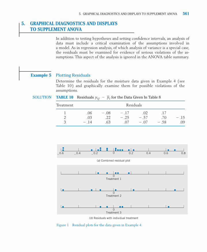
5. GRAPHICAL DIAGNOSTICS AND DISPLAYS TO SUPPLEMENT ANOVA 561
TABLE 10 Residuals for the Data Given In Table 8
Treatment Residuals
1 .06 � .08 � .17 .02 .172 .03 .22 � .25 � .57 .70 � .153 � .14 .63 .07 � .07 � .58 .09
y i j � y i
0_0.6 _0.4 _0.2 0.2 0.4 0.6 0.8
0
0
Treatment 1
Treatment 2
0Treatment 3
(b) Residuals with individual treatment
(a) Combined residual plot
Figure 1 Residual plots for the data given in Example 4.
5. GRAPHICAL DIAGNOSTICS AND DISPLAYS TO SUPPLEMENT ANOVA
In addition to testing hypotheses and setting confidence intervals, an analysis ofdata must include a critical examination of the assumptions involved ina model. As in regression analysis, of which analysis of variance is a special case,the residuals must be examined for evidence of serious violations of the as-sumptions. This aspect of the analysis is ignored in the ANOVA table summary.
Example 5 Plotting ResidualsDetermine the residuals for the moisture data given in Example 4 ( seeTable 10) and graphically examine them for possible violations of theassumptions.
SOLUTION
c14.qxd 10/15/09 11:36 AM Page 561

The residual plots of these data are shown in Figure 1, where the combined dotdiagram is presented in (a) and the dot diagrams of residuals corresponding toindividual treatments appear in (b).
From an examination of the dot diagrams, the variability in the points fortreatment 1 appears to be somewhat smaller than the variabilities in thepoints for treatments 2 and 3. However, given so few observations, it is diffi-cult to determine if this has occurred by chance or if treatment 1 actuallyhas a smaller variance. A few more observations are usually necessary toobtain a meaningful pattern for the individual treatment plots.
Fortunately, the ANOVA testing procedure is robust in the sense thatsmall or moderate departures from normality and constant variance do notseriously affect its performance.
In addition to the ANOVA a graphical portrayal of the data, as a box plotfor each treatment, conveys important information available for making com-parisons of populations.
Example 6 Box Plots Reveal Differences between PopulationsThe sepal width was measured on 50 iris flowers for each of three varieties,Iris setosa, Iris versicolor, and Iris virginica. A computer calculation producedthe summary shown in the following ANOVA table.
562 CHAPTER 14/ANALYSIS OF VARIANCE (ANOVA)
Source SS d.f. F
Treatment 11.345 2 49.16Error 16.962 147
Total 28.307 149
Treatment Sample Mean
Iris setosa 3.428Iris versicolor 2.770Iris virginica 2.974
Since (2, 147) � 3.05, we reject the null hypothesis of equal sepalwidth means at the 5% level of significance.
F.05
A calculation of multiple-t confidence intervals shows that all populationmeans differ from one another (see Exercise 14.36). Display the data on thethree varieties in boxplots.
c14.qxd 10/15/09 11:36 AM Page 562

SOLUTION The data are given in Exercise 14.36. Boxplots graphically display the varia-tion in the sepal width measurements. From Figure 2, we see that the Irissetosa typically has larger sepal width. R. A. Fisher, who developed analysis ofvariance, used these data along with other lengths and widths to introducea statistical technique for identifying varieties of plants.
6. RANDOMIZED BLOCK EXPERIMENTS FOR COMPARING k TREATMENTS
Just as we can pair like subjects or experimental units to improve upon the pro-cedure of taking two independent samples, we can also arrange, or block subjectsinto homogeneous groups of size k when comparing k treatments. Then if eachtreatment is applied to exactly one unit in the block and comparisons are onlydrawn between treatment responses from the same block, extraneous variabilityshould be greatly reduced. It is this concept of blocking that underlies therandomized block design.
The term “block design” originated from the design of agricultural fieldtrials, where “block” refers to a group of adjacent plots. A few typical exam-ples for which the block design may be appropriate are clinical trials to com-pare several competing drugs, where the experimental subjects are groupedin blocks according to age group and severity of symptoms; psychological ex-periments comparing several stimuli, where subjects may be blocked accord-ing to socioeconomic background; and comparison of several techniques forstoring fruit or vegetables, where each incoming shipment is regarded as ablock.
As its name implies, randomization is a basic part of the block design. Thistime, once the grouping of like experimental subjects in blocks is accom-plished, we randomly select one subject from the first block to receive treat-ment 1, one of the remaining subjects to receive treatment 2, and so on. Thesame procedure is repeated with a new randomization for each of the remain-ing blocks.
6. RANDOMIZED BLOCK EXPERIMENTS FOR COMPARING k TREATMENTS 563
2 3 4 5Width
Iris setosa
Iris versicolor
Iris virginica
Figure 2 Boxplots for the three iris samples.
c14.qxd 10/15/09 11:36 AM Page 563

Once the data are obtained, they can be arranged in rows according to thetreatments and in columns according to the blocks. If we designate the mea-surement corresponding to treatment i and block j by , the data structure of arandomized block design with b blocks and k treatments is shown in Table 11. The
y i j
row and column means are denoted by
and the overall mean, or
These means are shown in the margins of the table. Here an overbar on y indi-cates an average and a dot in the subscript denotes that the average is taken overthe subscript appearing in that place.
We now discuss the analysis of variance for a randomized block design withillustrative calculations based on the data given in Example 7.
Example 7 The Structure of Data from a Randomized Block ExperimentThe cutting speeds of four types of tools are being compared in an experiment.Five materials of varying degrees of hardness are to be used as experimentalblocks. The data pertaining to measurements of cutting time in seconds appearin Table 12.
grand mean y . . �1b k
�k
i � 1 �
b
j � 1 y i j
jth block (column) mean y . j �1k
�k
i � 1 y i j
ith treatment (row) mean y i
. �1b
�b
j � 1 y i j
564 CHAPTER 14/ANALYSIS OF VARIANCE (ANOVA)
TABLE 11 Data Structure of a Randomized Block Design with b Blocks and k Treatments
Block Block Block Treatment1 2 � � � b Means
Treatment 1 � � �Treatment 2 � � �
� � � � � � � �� � � � � � � �� � � � � � � �
Treatment k � � �
Block means � � � y .
.y
. by
. 2y
. 1
y k .y k by k2y k1
y 2 .y 2 by 22y 21
y1.y 1by 12y 11
c14.qxd 10/15/09 11:36 AM Page 564

6. RANDOMIZED BLOCK EXPERIMENTS FOR COMPARING k TREATMENTS 565
TABLE 12 Measurements of Cutting Time According to Types of Tool (Treatments) and Hardness of Material (Blocks)
Block TreatmentTreatment 1 2 3 4 5 Means
1 12 2 8 1 72 20 14 17 12 173 13 7 13 8 144 11 5 10 3 6
Block means y . . �20020
� 10y . 5 � 11y .
4 � 6y . 3 � 12y .
2 � 7y . 1 � 14
y4. � 7y3. � 11y2. � 16y1. � 6
Decomposition of Observations
� � � Residual
� � � � ( y i j � y i . � y . j � y . .
)( y. j � y . .)( y i . � y . . )y . .y i j
Deviationdue toblock
Deviationdue to
treatmentObservation �
Grandmean
TABLE 13 Decomposition of Observations for the Randomized Block Experiment in Table 12
� �
� �
� �20
�20
�11
�11
0�1
01
�1010
002
�2�� �
4444
�3�3�3�3
2222
�4�4�4�4
1111�
Residualy i j � y i
. � y . j � y . .
BlockEffect
y . j � y . .
� ��4
61
�3
�461
�3
�461
�3
�461
�3
�461
�3�� �
10101010
10101010
10101010
10101010
10101010��
12201311
21475
8171310
11283
717146�
TreatmentEffect
y i . � y . .
Grand Meany . .
Observationy i j
The observations form a two-way table, and their decomposition indicatesboth a term for row (treatment) deviations and column (block) deviations.
c14.qxd 10/15/09 11:36 AM Page 565

566 CHAPTER 14/ANALYSIS OF VARIANCE (ANOVA)
The number of distinct entries in the treatment effects array is k,and the single constraint is that they must sum to zero. Thus, k � 1 degrees offreedom are associated with the treatment sum of squares.
y i . � y . .
Sum of Squares Due to Treatment
with d.f. � k � 1.
� b �k
i � 1 ( y i
. � y . .
)
2
SST � �k
i � 1 �
b
j � 1 ( y i
. � y . . )2
TABLE 14 An Alternative Format of the Decomposition Table for a Randomized Block Experiment
Deviation ofBlock Treatment Mean
Treatment 1 � � � j � � � b from Grand Mean
1� � �� � �� � �i � � � � � �
� � �� � �� � �k
� � � � � �Grand mean
y . .( y .
b � y . . )( y.
j � y . .
)( y.1 � y..)Deviation ofblock mean
from grand mean
( y k . � y . .
)
( y i . � y . .
)( y i j � y i . � y.
j � y. . )
( y1 . � y . .
)
Taking the observation � 12 in Example 7, we obtain
Table 13 contains the results of the decomposition of all the observations. Table 14gives an alternative format.
� 10 � ( � 4 ) � ( 4 ) � ( 2 )
12 � 10 � ( 6 � 10 ) � ( 14 � 10 ) � ( 12 � 14 � 6 � 10 )
y 11
c14.qxd 10/15/09 11:36 AM Page 566

6. RANDOMIZED BLOCK EXPERIMENTS FOR COMPARING k TREATMENTS 567
In the array of treatment effects in Table 13, each entry appears b � 5 times,once in each block. The treatment sum of squares for this example is then
with d.f. � 4 � 1 � 3.In a similar manner, we obtain the block sum of squares.
SST � 5 ( �4 )2 � 5 ( 6 )2 � 5 ( 1 )
2 � 5 ( �3 )
2 � 310
Sum of Squares Due to Block
with d.f. � b � 1.
� k �b
j � 1 ( y.j � y.. )2
SSB � �k
i � 1 �
b
j � 1 ( y.j � y.. )2
Residual Sum of Squares or Error Sum of Squares
with d.f. � (b � 1)(k � 1).
SSE � �k
i � 1 �
b
j � 1 ( y i j � y i
. � y . j � y . . )2
Referring to the array of block effects in Table 13, we find the block sum ofsquares for our example to be
with d.f. � 5 � 1 � 4.The number of degrees of freedom associated with the residual array is
( b � 1)( k � 1). To understand why this is so, note that among the b � kresiduals, the following constraints are satisfied. One constraint is that thesum of all entries must be zero. The fact that all row sums are zero introducesk � 1 additional constraints. This is so because having fixed any k � 1 rowtotals and the grand total, the remaining row total is automatically fixed. Bythe same reasoning, b � 1 additional constraints arise from the fact that allcolumn totals are zero. Consequently, the number of degrees of freedom forthe residual is
b k � 1 � ( k � 1 ) � ( b � 1 ) � ( b � 1 )( k � 1 )
SSB � 4 ( 4 )2 � 4 ( �3 )2 � 4 ( 2 )2 � 4 ( �4 )2 � 4 ( 1 )2 � 184
c14.qxd 10/15/09 11:36 AM Page 567

568 CHAPTER 14/ANALYSIS OF VARIANCE (ANOVA)
TABLE 15 ANOVA Table for a Randomized Block Design
Source Sum of Squares d.f. Mean Square F-Ratio
Treatments k � 1
Blocks b � 1
Residual (b � 1)(k � 1)
Total bk � 1�k
i � 1 �
b
j � 1 ( y i j � y . . )2
MSE �SSE
( b � 1 )( k � 1 )SSE � �
k
i � 1 �
b
j � 1( y i j � y i .� y .
j � y . . )2
MSB
MSEMSB �
SSB
b � 1SSB � k �
b
j � 1 ( y .
j � y . . )2
MST
MSEMST �
SST
k � 1SST � b �
k
i � 1 ( y i
. � y . . )2
TABLE 16 ANOVA Table for the Data Given in Example 7
Sum of MeanSource Squares d.f. Square F-Ratio
Treatments 310 3 103.3 51.7Blocks 184 4 46 23Residual 24 12 2
Total 518 19
In our example,
with d.f. � ( 5 � 1)( 4 � 1 ) � 12.Finally, the total sum of squares equals the sum of squares of each observa-
tion about the grand mean, or
with d.f. � bk � 1. In our example, we sum the square of each entry in thearray for and subtract the sum of squares of entries in the array.
With d.f. � (5)(4) � 1 � 19.This provides a check on our previous calculations,because those sums of squares and degrees of freedom must sum to these totals.
These calculations are conveniently summarized in the ANOVA tables shownin Table 15 for the general case and Table 16 for the data in our numerical example.The last column of F-ratios will be explained after we discuss the population model.
� 518
�[ ( 10 )
2 � ( 10 )2 � ��� � ( 10 )
2 ]
Total sum of squares � ( 12 )2 � ( 2 )2 � ��� � ( 6 )
2
y . .y i j
Total sum of squares � �k
i � 1 �
b
j � 1 ( y i j � y . .
)2 � �k
i � 1 �
b
j � 1 y
2
i j � b k y2 . .
SSE � 22 � 0
2 � ( �2 )
2 � 0
2 � ��� � ( �2 )
2 � 24
c14.qxd 10/15/09 11:36 AM Page 568

Again, a statistical test of treatment differences is based on an underlyingpopulation model.
6. RANDOMIZED BLOCK EXPERIMENTS FOR COMPARING k TREATMENTS 569
Population Model for a Randomized Block Experiment
� m � � �
for i � 1, . . . , k and j � 1, . . . , b, where the parameters satisfy
and the ei j are random errors independently distributed as N(0, s).
�k
i � 1 � i � 0 �
b
j � 1 j � 0
e i j j� iY
i j
Observation �Overallmean
�Treatment
effect�
Blockeffect
� Error
Reject � � � � � � � 0 (no treatment differences) if
Reject � � � � � � � 0 (no block differences) if
MSB
MSE� F�( b � 1, ( b � 1 ) ( k � 1 ) )
b 1H0
MST
MSE� F�( k � 1, ( b � 1 )( k � 1 ) )
� k� 1H0
Tests for the absence of treatment differences or differences in block effectscan now be performed by comparing the corresponding mean square with theyardstick of the error mean square by using an F test.
To test the hypothesis of no treatment differences for the analysis of vari-ance in Table 16, we find that the tabulated .05 point of F (3, 12) is 3.49, a valuefar exceeded by the observed F-ratio for treatment effect. We therefore con-clude that a highly significant treatment difference is indicated by the data. Theblock effects are also highly significant, because the observed F value of 23 ismuch larger than the tabulated value (4, 12) � 3.26.
Again, we stress that a serious violation of the model assumptions is likely tojeopardize the conclusions drawn from the preceding analyses and a careful exami-nation of the residuals should be an integral part of the analysis. In addition to plot-ting the whole set of residuals in a graph, separate plots for individual treatmentsand individual blocks should also be studied. When observations are collected overtime, a plot of the residuals versus the time order is also important.
F.05
c14.qxd 10/15/09 11:36 AM Page 569

570 CHAPTER 14/ANALYSIS OF VARIANCE (ANOVA)
CONFIDENCE INTERVALS FOR TREATMENT DIFFERENCES
In addition to performing the overall F test for detecting treatment differences,the experimenter typically establishes confidence intervals to compare specificpairs of treatments. This is particularly important when the F test leads to a rejec-tion of the null hypothesis, thus signifying the presence of treatment differences.
We next estimate the difference � of the mean responses of treat-ments i and i. Because is normally distributed with a mean of �
and a variance of
the ratio
has a t distribution with d.f. � (b � 1)(k � 1). This result can be used toconstruct a confidence interval for an individual difference � .
When several such pairwise comparisons are to be integrated into a com-bined confidence statement, the concept of simultaneous confidence intervals,discussed in Section 4, is again applied.
Exercises
� i� i
T �( Yi
. � Y i
.
) � ( � i � � i
)
√ MSE √ 2 / b
�
2 �
1b
�1b
� � �2 �
2b
�� i
� iY i . � Y i
.� i� i
BlockTreatment 1 2 3 4
1 11 10 7 02 7 8 7 23 15 6 13 10
BlockTreatment 1 2 3 4
1 35 24 28 212 19 14 14 133 21 16 21 14
14.22 Suppose you wish to compare three differentbrands of tick collars for dogs. You have availablethree of each of the breeds Poodle, Lab, Collie,and Dachshund. Explain how you would assign abrand of tick collar to each of the 12 dogs in or-der to conduct a randomized block experiment.
14.23 The hours of relief are measured under aplacebo, Brand A, and Brand B sinus medicines.Call these treatment 1, treatment 2, and treat-ment 3, respectively. They are each given insuccession, in random order, to a subject withtwo days between each treatment. Supposethe data are
(a) Provide a decomposition for the observationsfrom this randomized block experiment.
(b) Find the sum of squares for each array.
(c) Determine the degrees of freedom bychecking the constraints for each array.
14.24 The yield, in pounds, of three types of heritagetomatoes is obtained after planting them inthree equal sized plots within a site. The assign-ment of type to a plot is random. A total of fourdifferent sites are used. Suppose the data are
(a) Provide a decomposition for the observationsfrom this randomized block experiment.
c14.qxd 10/15/09 11:36 AM Page 570

(b) Find the sum of squares for each array.
(c) Determine the degrees of freedom bychecking the constraints for each array.
14.25 Refer to Exercise 14.23. Present the ANOVAtable. What conclusions can you draw from thetwo F tests? Take a � .05.
14.26 Refer to Exercise 14.24. Present the ANOVAtable. What conclusions can you draw from thetwo F tests? Take a � .05.
14.27 Three loaves of bread, each made according toa different recipe, are baked in one oven at thesame time. Because of possible uncontrolledvariations in oven performance, each baking istreated as a block. This procedure is repeatedfive times, and the following measurements ofdensity are obtained.
USING STATISTICS WISELY 571
(b) Perform an analysis of variance for thesedata.
14.28 Referring to Exercise 14.27:
(a) Obtain simultaneous confidence intervalsfor the pairwise differences in mean den-sity for the three recipes. Take a � .05.
(b) Calculate the residuals and make a normal-scores plot.
14.29 As part of a cooperative study on the nutri-tional quality of oats, 6 varieties of oat kernelswith their hulls removed are subjected to amineral analysis. The plants are grown accord-ing to a randomized block design, and themeasurements of protein by percent of dryweight are recorded in Table 17.
(a) Perform an analysis of variance for thesedata.
(b) Calculate and plot the residuals. Does themodel appear to be adequate?
14.30 Referring to Exercise 14.29, suppose that vari-ety 6 is of special interest. Construct simultane-ous 90% confidence intervals for the differencesbetween the mean of variety 6 and each of theother means.
BlockTreatment 1 2 3 4 5 6
1 19.09 20.29 20.31 19.60 18.62 20.102 16.28 17.88 16.88 17.57 16.72 17.323 16.31 18.17 17.38 17.53 16.34 17.884 17.50 18.05 17.59 17.64 17.38 18.045 16.25 16.92 15.88 14.78 15.97 16.666 21.09 21.37 21.38 20.52 21.09 21.58
Data courtesy of D. Peterson, L. Schrader, and V. Youngs.
USING STATISTICS WISELY
1. When collecting data according to a one-way ANOVA design, conductthe trials in random order if at all possible.
2. Do not routinely accept the analysis of variance generated by statisticalsoftware. Instead, inspect the residuals for outliers or patterns indicatingthat the variance is not constant across treatments.
BlockRecipe 1 2 3 4 5
1 .95 .86 .71 .72 .742 .71 .85 .62 .72 .643 .69 .88 .51 .73 .44
(a) How should the three oven positions ofthe three loaves be selected for each trial?
TABLE 17 Protein (prct. dry wt.)
c14.qxd 10/15/09 11:36 AM Page 571

KEY IDEAS AND FORMULAS
Several populations can be compared using the Analysis of variance (ANOVA).A completely randomized design specifies taking independent random sam-
ples from each population.All of the observations are assumed to have a common variance. Then the
ANOVA consists of a separation of the total sum of squares into componentsdue to different sources of variation.
When samples are taken from k populations the two sources of variation arethe within population variation or error and the differences between populationmeans or treatments. The jth observation on the ith treatment is . The errorvariation is estimated using the residuals or � which are the deviations ofthe observations from their respective sample means.
The total variation in the observations is expressed as
Total sum of squares
is partitioned into the two components:
1. Treatment sum of squares:
2. Error sum of squares:
This decomposition of sums of squares is summarized in an analysis of variance(ANOVA) table. This table includes the mean square for each sum of squares.
Mean square
The F statistic � ( Treatment mean square ) / ( Error mean square )
which has an F distribution with k � 1 and n � k degrees of freedom.To ensure an overall confidence level for all confidence intervals, it is desirable to
use a simultaneous (multiple) confidence intervals procedure when calculating con-fidence intervals for the many mean differences. The multiple-t confidence intervalsfor all m � k (k � 1)/2 statements about the mean differences � are
Fortunately, the one-way analysis of variance is robust with respect to small ormoderate departures from the assumptions of normal errors with common variance.
� Y i � Y i � t� / 2m �
MSEn � k
, Y i � Y i � t� / 2 m �
MSEn � k
��i�i
�Sum of squares
Degrees of freedom
SSE � �k
i � 1 �
n i
j � 1 ( y i j � y i
)2
SST � �k
i � 1 n i( y i � y )2
�k
i � 1 �
n i
j � 1 ( y i j � y )2
� �k
i � 1 �
n i
j � 1 ( y i j � y )2
y i j
y iy i j
y i j
572 CHAPTER 14/ANALYSIS OF VARIANCE (ANOVA)
c14.qxd 10/15/09 11:36 AM Page 572

The technique of blocking, or grouping experimental units into homogeneoussets, can reduce extraneous variation and sharpen comparisons among treatments.
The analysis of variance of a randomized block experiment is based on the
partition of the total sum of squares into three components:
1. Treatment sum of squares:
2. Block sum of squares:
3. Error sum of squares:
TECHNOLOGY
One-way analysis of variance (ANOVA)
MINITAB
We illustrate with the data from different populations in separate columns. Forexample, with data from 3 populations in columns C1, C 2, and C 3:
Data
C1: 6 10 8C2: 13 14 15 14C3: 3 7 5
Stat Q ANOVA Q One-way (Unstacked)Type C1–C3 in Responses (in separate columns:)Click on Graphs. Select Three in one. Click OK.Click OK.
In addition to the analysis, this produces a histogram of the residuals as well as aplot of residuals versus fitted values.
EXCEL
Enter the data from the different populations in separate columns, for instanceA, B, C, etc., with a label in the first cell of each column.
SSE � �k
i � 1 �
b
j � 1 ( y i j � y i
. � y . j � y . .
)2
SSB � k �b
j � 1 ( y .
j � y . . )2
SST � b �k
i � 1 ( y i
. � y . .
)2
�k
i � 1�b
j � 1( y i j � y . . )2
TECHNOLOGY 573
c14.qxd 10/15/09 11:36 AM Page 573

Select Tools, then Data Analysis. Select Statistical and then Anova:SingleFactor.Click OK. Highlight the columns and check Labels in First Row.Enter Alpha and click OK.
The output includes the ANOVA table and P–value for test of equality ofthe means.
TI-84/-83 PLUS
Store the data in lists, one for each population. With 3 populations enter data inL1, L2, and L3.
Select STAT Q TESTS Q ANOVA.Enter L1, L2, L3 and close the parenthesis to obtain ANOVA(L1, L2, L3).Press Enter.
The software returns the value of the F statistic and the P–value, along withother values from the ANOVA table.
7. REVIEW EXERCISES
574 CHAPTER 14/ANALYSIS OF VARIANCE (ANOVA)
Treatment 1 Treatment 2 Treatment 3
19 16 1318 11 1621 13 1818 14 11
11 1511
Fabric 1 Fabric 2 Fabric 3 Fabric 4
17.8 11.2 11.8 14.916.2 11.4 11.0 10.817.5 15.8 10.0 12.817.4 10.0 9.2 10.715.0 10.4 9.2 10.7
14.31 Food scientists investigated whether making acheese sauce by a continuous process or batchprocess made any difference to taste. They alsoincluded a third treatment, a carefully selectedideal product, that served as a control. Treatment1 is the ideal, treatment 2 is the continuousprocess, and treatment 3 is the batch process.Suppose the sensory ratings by trained testers are
14.33 Using the table of percentage points for the Fdistribution, find(a) The upper 5% point when d.f. � (7, 13).(b) The upper 5% point when d.f. � (7, 20).(c) The upper 10% point when d.f. � (7, 12).
14.34 As part of the multilab study, four fabrics aretested for flammability at the National Bureau ofStandards. The following burn times in secondsare recorded after a paper tab is ignited on thehem of a dress made of each fabric.
Provide a decomposition for the observationsabove from a completely randomized designwith three treatments.
14.32 Compute the sums of squares and constructthe ANOVA table for the data given in Exer-cise 14.31.
(a) State the statistical model and present theANOVA table. With a � .05, test the nullhypothesis of no difference in the degree offlammability for the four fabrics.
c14.qxd 10/15/09 11:36 AM Page 574

7. REVIEW EXERCISES 575
Data
C1: 10 15 8 12 15C2: 14 18 21 15C3: 17 16 14 15 17 15 18C4: 12 15 17 15 16 15
Dialog box:
Stat Q ANOVA Q One-way ( nstacked)Type C1-C4 in Responses. Click OK.
U
The Output is as follows:
One-way ANOVA: C1, C2, C3, C4
SOURCE DF SS MS F PFACTOR 3 68.00 22.67 4.34 0.018ERROR 18 94.00 5.22TOTAL 21 162.00
S = 2.285 R-Sq= 41.98%
LEVEL N MEAN STDEVC1 5 12.000 3.082C2 4 17.000 3.162C3 7 16.000 1.414C4 6 15.000 1.673
POOLED STDEV = 2.285
INDIVIDUAL 95% CIS FOR MEAN BASED ON POOLED STDEV
–+––––––--+––––––--+––––––--+––––––––(––––––*––––––)
(–––––––*–––––––)(–––––*–––––)
(––––––*––––––)––––––––+–––––––––+–––––––––+––––––––
10.0 12.5 15.0 17.5
Use computer software to analyze the mois-ture data in Table 8.
14.36 The iris data described in Example 6are given in the stem-and-leaf diagrams below.
The MINITAB output for the analysis of theiris data is given below.
LEAF UNIT � 0.10
SETOSA VERSICOLOR VIRGINICA
2 0
2 3 2 22333 2 2
2 2 4445555 2 5555
2 2 66677777 2 667777
2 9 2 8888889999999 2 8888888899
3 0000001111 3 00000000111 3 0000000000001111
3 2222233 3 2223 3 22222333
3 444444444555555 3 4 3 44
3 666777 3 6
3 888899 3 88
4 01
4 2
4 4
One-way ANOVA:
SOURCE DF SS MS F PIRIS 2 11.345 5.672 49.16 0.000ERROR 147 16.962 0.115TOTAL 149 28.307
S = 0.3397 R-Sq = 40.08%
(b) If the null hypothesis is rejected, con-struct simultaneous confidence intervalsto determine the fabric(s) with the lowestmean burn time.
(c) Plot the residuals and comment on theplausibility of the assumptions.
(d) If the tests had been conducted one at atime on a single mannequin, how wouldyou have randomized the fabrics tested inthis experiment?
The Following Exercises Require a Computer
14.35 Using the computer. MINITAB can be usedfor ANOVA. Start with the data on each treat-ment, from Example 1, set in separate columns.The sequence of commands and output is:
c14.qxd 10/15/09 11:36 AM Page 575
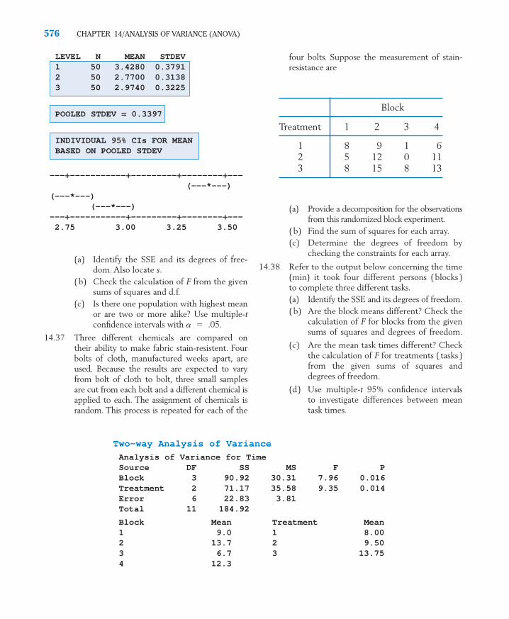
576 CHAPTER 14/ANALYSIS OF VARIANCE (ANOVA)
Two-way Analysis of Variance
Analysis of Variance for TimeSource DF SS MS F PBlock 3 90.92 30.31 7.96 0.016Treatment 2 71.17 35.58 9.35 0.014Error 6 22.83 3.81Total 11 184.92
Block Mean Treatment Mean1 9.0 1 8.002 13.7 2 9.503 6.7 3 13.754 12.3
LEVEL N MEAN STDEV1 50 3.4280 0.37912 50 2.7700 0.31383 50 2.9740 0.3225
POOLED STDEV = 0.3397
INDIVIDUAL 95% CIs FOR MEAN BASED ON POOLED STDEV
–––+–––––-–––––+–––––––––+––––––––+–––(–––*–––)
(–––*–––)(–––*–––)
–––+–––––––––––+–––––––––+––––––––+–––2.75 3.00 3.25 3.50
(a) Identify the SSE and its degrees of free-dom. Also locate s.
(b) Check the calculation of F from the givensums of squares and d.f.
(c) Is there one population with highest meanor are two or more alike? Use multiple-tconfidence intervals with a � .05.
14.37 Three different chemicals are compared ontheir ability to make fabric stain-resistent. Fourbolts of cloth, manufactured weeks apart, areused. Because the results are expected to varyfrom bolt of cloth to bolt, three small samplesare cut from each bolt and a different chemical isapplied to each. The assignment of chemicals israndom. This process is repeated for each of the
four bolts. Suppose the measurement of stain-resistance are
Block
Treatment 1 2 3 4
1 8 9 1 62 5 12 0 113 8 15 8 13
(a) Provide a decomposition for the observationsfrom this randomized block experiment.
(b) Find the sum of squares for each array.(c) Determine the degrees of freedom by
checking the constraints for each array.
14.38 Refer to the output below concerning the time(min) it took four different persons (blocks )to complete three different tasks.(a) Identify the SSE and its degrees of freedom.(b) Are the block means different? Check the
calculation of F for blocks from the givensums of squares and degrees of freedom.
(c) Are the mean task times different? Checkthe calculation of F for treatments ( tasks )from the given sums of squares anddegrees of freedom.
(d) Use multiple-t 95% confidence intervalsto investigate differences between meantask times.
c14.qxd 10/15/09 11:36 AM Page 576

1. Introduction2. The Wilcoxon Rank-Sum Test
for Comparing Two Treatments3. Matched Pairs Comparisons4. Measure of Correlation Based on Ranks5. Concluding Remarks6. Review Exercises
15
Nonparametric Inference
c15.qxd 10/15/09 11:37 AM Page 577

Selecting the Best Vintage
Wines can be ranked without reference to a quantitative scale of measurement. Individuals use non-quantitative characteristics to help select their favorite wines.© Peter Beck/Corbis Stock Market.
Using their professional judgment, wine critics do give a numeral rating as a guide to overall quali-tative placement and wine quality. However, ratings among critics differ on the same bottle ofwine and even the meaning of 90 points on one scale is different from that of 90 points on an-other critic’s scale. Ratings can never substitute for your own palate or your own wine tastingrankings.
c15.qxd 10/15/09 11:37 AM Page 578

1. INTRODUCTION
Nonparametric refers to inference procedures that do not require the popula-tion distribution to be normal or some other form specified in terms of para-meters. Nonparametric procedures continue to gain popularity because theyapply to a very wide variety of population distributions. Typically, they utilizesimple aspects of the sample data, such as the signs of the measurements, orderrelationships, or category frequencies. Stretching or compressing the scale ofmeasurement does not alter them. As a consequence, the null distribution of anonparametric test statistic can be determined without regard to the shape ofthe underlying population distribution. For this reason, these tests are alsocalled distribution-free tests. This distribution-free property is their strongestadvantage.
What type of observations are especially suited to a nonparametric analysis?Characteristics like degree of apathy, taste preference, and surface gloss cannotbe evaluated on an objective numerical scale, and an assignment of numbers is,therefore, bound to be arbitrary. Also, when people are asked to express theirviews on a five-point rating scale,
the numbers have little physical meaning beyond the fact that higher scoresindicate greater agreement. Data of this type are called ordinal data, becauseonly the order of the numbers is meaningful and the distance between the twonumbers does not lend itself to practical interpretation. Nonparametric proce-dures that utilize information only on order or rank are particularly suited tomeasurements on an ordinal scale.
2. THE WILCOXON RANK-SUM TEST FOR COMPARING TWO TREATMENTS
The problem of comparing two populations based on independent randomsamples has already been discussed in Section 2 of Chapter 10. Under theassumption of normality and equal standard deviations, the parametric inferenceprocedures were based on Student’s t statistic. Here we describe a usefulnonparametric procedure named after its proposer F. Wilcoxon (1945). Anequivalent alternative version was independently proposed by H. Mann and D. Whitney (1947).
2. THE WILCOXON RANK-SUM TEST FOR COMPARING TWO TREATMENTS 579
1
StronglyDisagree Disagree Indifferent Agree
StronglyAgree
2 3 4 5
c15.qxd 10/15/09 11:37 AM Page 579

For a comparative study of two treatments A and B, a set of n � �experimental units is randomly divided into two groups of sizes and ,respectively. Treatment A is applied to the units, and treatment B to theother units. The response measurements, recorded in a slightly differentnotation than before, are
Treatment A , , . . . ,
Treatment B , , . . . ,
These data constitute independent random samples from two populations.Assuming that larger responses indicate a better treatment, we wish to test thenull hypothesis that there is no difference between the two treatment effectsversus the one-sided alternative that treatment A is more effective than treat-ment B. In the present nonparametric setting, we only assume that the distribu-tions are continuous.
Note that no assumption is made regarding the shape of the population distribu-tion. This is in sharp contrast to our t test in Chapter 10, where we assumedthat the population distributions were normal with equal standard deviations.Figure 1 illustrates the above hypotheses and .
The basic concept underlying the rank-sum test can now be explained bythe following intuitive line of reasoning. Suppose that the two sets of observa-tions are plotted on the same diagram using different markings A and B to iden-tify their sources. Under , the samples come from the same population, soH0
H1H0
YnBY2Y1
XnAX2X1
nB
nA
nBnA
nBnA
580 CHAPTER 15/NONPARAMETRIC INFERENCE
Figure 1 (a) Null distribution. (b) A shift alternative.
Model: Both Population Distributions Are Continuous
Hypotheses
: The two population distributions are identical.
: The distribution of population A is shifted to the right of the distri-bution of population B.
H1
H0
Identical distributionof both populations
Shift of amount
Population B Population A
∆
H0 H1
(a) (b)
c15.qxd 10/15/09 11:37 AM Page 580

that the two sets of points should be well mixed. However, if the larger obser-vations are more often associated with the first sample, for example, we can infer that population A is possibly shifted to the right of population B. Thesetwo situations are diagrammed in Figure 2, where the combined set of points ineach case is serially numbered from left to right. These numbers are called thecombined sample ranks. In Figure 2a, large as well as small ranks are associatedwith each sample, whereas in Figure 2b, most of the larger ranks are associ-ated with the first sample. Therefore, if we consider the sum of the ranks as-sociated with the first sample as a test statistic, a large value of this statisticshould reflect that the first population is located to the right of the second.
To establish a rejection region with a specified level of significance, we mustconsider the distribution of the rank-sum statistic under the null hypothesis.This concept is explored in Example 1, where small sample sizes are investi-gated for easy enumeration.
Example 1 Determining the Null Distribution of the Rank-Sum StatisticTo determine if a new hybrid seedling produces a bushier flowering plantthan a currently popular variety, a horticulturist plants 2 new hybridseedlings and 3 currently popular seedlings in a garden plot. After the plantsmature, the following measurements of shrub girth in inches are recorded.
Shrub Girth (in inches)Treatment A 31.8 39.1(new hybrid)
Treatment B 35.5 27.6 21.3(current variety)
Do these data strongly indicate that the new hybrid produces larger shrubsthan the current variety?
SOLUTION We wish to test the null hypothesis
: A and B populations are identical
versus the alternative hypothesis
: Population A is shifted from B toward larger valuesH1
H0
A B A A A AB B B
1 2 3 6 8 94 5 7
(a)
Ranks
B B B A A AA B A
1 2 3 6 8 94 5 7
(b)
Ranks
Figure 2 Combined plot of the two samples and the combined sample ranks. (a) Mixed ranks. (b) Higher ranksare mostly A.
2. THE WILCOXON RANK-SUM TEST FOR COMPARING TWO TREATMENTS 581
c15.qxd 10/15/09 11:37 AM Page 581

For the rank-sum test, the two samples are placed together and rankedfrom smallest to largest:
Combined sampleordered observations 21.3 27.6 31.8 35.5 39.1
Ranks 1 2 3 4 5
Treatment B B A B A
Rank sum for ARank sum for B
Because larger measurements and therefore higher ranks for treatment Atend to support , the rejection region of our test should consist of largevalues for :
To determine the critical value c so that the Type I error probability is con-trolled at a specified level a, we evaluate the probability distribution of under . When the two samples come from the same population, every pair of integers out of { 1, 2, 3, 4, 5 } is equally likely to be the ranks for the two
A measurements. There are potential pairs, so that each collection
of possible ranks has a probability of under . These rank collec-tions are listed in Table 1 with their corresponding values. The null distribu-tion of can be obtained immediately from Table 1 by collecting theprobabilities of identical values (see Table 2). The observed value � 8WA
WA
WA
H01
10 � .1
� 52
� � 10
H0
WA
Reject H0 if WA � c
WA
H1
WB � 1 � 2 � 4 � 7
WA � 3 � 5 � 8
582 CHAPTER 15/NONPARAMETRIC INFERENCE
TABLE 1 Rank Collections for Treatment A with Sample Sizes � 2, � 3
Ranks of A Rank Sum Probability
1,2 3 .11,3 4 .11,4 5 .11,5 6 .12,3 5 .12,4 6 .12,5 7 .13,4 7 .13,5 8 .14,5 9 .1
Total 1.0
WA
nBnA
c15.qxd 10/15/09 11:37 AM Page 582

has the significance probability In otherwords, we must tolerate a Type I error probability of .2 in order to reject .Therank-sum test leads us to conclude that the evidence is not sufficiently strong toreject . Note that even if the A measurements did receive the highest ranks of4 and 5, a significance level of a � .1 would be required to reject .
Guided by Example 1, we now state the rank-sum test procedure in a gen-eral setting.
A determination of the null distribution of the rank-sum statistic by directenumeration becomes more tedious as the sample sizes increase. However,tables for the null distribution of this statistic have been prepared for small sam-ples, and an approximation is available for large samples. To explain the use ofAppendix B, Table 7, first we note some features of the rank sums and .
The total of the two ranks sums � is a constant, which is the sumof the integers 1, 2, . . . , n, where n is the combined sample size. For instance,in Example 1,
� 1 � 2 � 3 � 4 � 5 � 15WA � WB � ( 3 � 5 ) � ( 1 � 2 � 4 )
WBWA
WBWA
H0
H0
H0
PH0 ( WA � 8 ) � .1 � .1 � .2.
TABLE 2 Distribution of the Rank Sum for Sample Sizes � 2, � 3
Value of 3 4 5 6 7 8 9
Probability .1 .1 .2 .2 .2 .1 .1
WA
nBnA
WA
Wilcoxon Rank-Sum Test
Let , . . . , and , . . . , be independent random samplesfrom continuous populations A and B, respectively. To test : The popu-lations are identical:
1. Rank the combined sample of n � � observations in increas-ing order of magnitude.
2. Find the rank sum of the first sample.
3. (a) For : Population A is shifted to the right of population B; setthe rejection region at the upper tail of .
(b) For : Population A is shifted to the left of population B; setthe rejection region at the lower tail of .
(c) For : Populations are different; set the rejection region atboth tails of having equal probabilities.WA
H1
WA
H1
WA
H1
WA
nBnA
H0
YnBY1XnA
X1
2. THE WILCOXON RANK-SUM TEST FOR COMPARING TWO TREATMENTS 583
c15.qxd 10/15/09 11:37 AM Page 583

Therefore, a test that rejects for large values of is equivalent to a test that rejects for small values of . We can just as easily designate thetest statistic and set the rejection region at the lower tail. Consequently, we canalways concentrate on the rank sum of the smaller sample and set the rejectionregion at the lower (or upper) tail, depending on whether the alternativehypothesis states that the corresponding population distribution is shifted to theleft (or right).
Second, the distribution of each of the rank-sum statistics and issymmetric. In fact, is symmetric about and issymmetric about Table 2 illustrates the symmetry ofthe distribution for the case This symmetry also holdsfor the test statistic calculated from the larger sample size.
THE USE OF APPENDIX B, TABLE 7
The Wilcoxon rank-sum test statistic is taken as
When the sample sizes are equal, take the sum of ranks for either of the sam-ples. Appendix B, Table 7 gives the upper- as well as the lower-tail probabilities:
Upper-tail probability
Lower-tail probability
By the symmetry of the distribution, these probabilities are equal when x and x*are at equal distances from the center. The table includes the x* values corre-sponding to the x’s at the upper tail.
Example 2 Using Table 7 in Appendix B to Set the Rejection RegionFind and when
SOLUTION From Table 7, we read opposite the entry x � 25, so .033 �
The lower tail entry is obtained by reading opposite x* � 8. We find illustrating the symmetryof .
P � P [WS � x ] � P [WS � x*]
WS
P [WS � 8] � .033P [WS � x*]P [WS � 8]
P [WS � 25].P � P [WS � x]
Larger sample size � 7
Smaller sample size � 3
P [WS � 8]P [WS � 25]
P [ WS � x* ]
P [ WS � x ]
WS � sum of ranks of the smaller sample in the combined sample ranking
nA � 2, nB � 3.WA
nB
( nA � nB � 1 ) / 2.WBnA
( nA � nB � 1 ) / 2WA
WBWA
WBWBH0
WAH0
584 CHAPTER 15/NONPARAMETRIC INFERENCE
c15.qxd 10/15/09 11:37 AM Page 584

The steps to follow when using Appendix B, Table 7 in performing a rank-sumtest are:
Use the rank-sum of the smaller sample as the test statistic. ( If the sam-ple sizes are equal, take either rank sum as .)
1. If states that the population corresponding to is shifted to theright of the other population, set a rejection region of the form �c and take c as the smallest x value for which P � a.
2. If states that the population corresponding to is shifted to theleft, set a rejection region of the form � c and take c as the largestx* value for which P � a.
3. If states that the population corresponding to is shifted in eitherdirection, set a rejection region of the form and read from the x* column and from the x column, so that P � a /2.
Example 3 Apply the Rank-Sum Test to Compare Two Geological FormationsTwo geological formations are compared with respect to richness of mineralcontent. The mineral contents of 7 specimens of ore collected from forma-tion 1 and 5 specimens collected from formation 2 are measured by chemicalanalysis. The following data are obtained:
Mineral Content
Formation 1 7.6 11.1 6.8 9.8 4.9 6.1 15.1
Formation 2 4.7 6.4 4.1 3.7 3.9
Do the data provide strong evidence that formation 1 has a higher mineralcontent than formation 2? Test with a near .05.
c2c1
WS � c1 or WS � c2
WSH1
WS
WSH1
WS
WSH1
WS
WS
Smaller Sample Size � 3, Larger Sample Size � 7
x P x*
22 — 1123 — 1024 — 9
: 25 .033 826 — 727 — 6
2. THE WILCOXON RANK-SUM TEST FOR COMPARING TWO TREATMENTS 585
c15.qxd 10/15/09 11:37 AM Page 585

SOLUTION To use the rank-sum test, first we rank the combined sample and determinethe sum of ranks for the second sample, which has the smaller size. Theobservations from the second sample and their ranks are underlined here forquick identification:
Combinedorderedvalues 4.9 6.1 6.8 7.6 9.8 11.1 15.1
Ranks 5 6 8 9 10 11 12
The observed value of the rank-sum statistic is
We wish to test the null hypothesis that the two population distributions areidentical versus the alternative hypothesis that the second population, corre-sponding to , lies to the left of the first. The rejection region is therefore atthe lower tail of .
Reading Appendix B, Table 7 with smaller sample size � 5 and larger sam-ple size � 7, we find and Hence, the rejection region with a � .053 is established as � 22.Because the observed value falls in this region, the null hypothesis is rejected ata � .053. In fact, it would be rejected if a were as low as � .009.
Example 4 Comparing Two Flame-Retardant MaterialsFlame-retardant materials are tested by igniting a paper tab on the hem of adress worn by a mannequin. One response is the vertical length of damage tothe fabric measured in inches. The following data (courtesy of B. Joiner) for5 samples, each taken from two fabrics, were obtained by researchers at theNational Bureau of Standards as part of a larger cooperative study.
Fabric A 5.7 7.3 7.6 6.0 6.5
Fabric B 4.9 7.4 5.3 4.6 6.2
Do the data provide strong evidence that a difference in flammability existsbetween the two fabrics? Test with a near .05.
SOLUTION The sample sizes are equal, so that we can take the rank sum of either sampleas the test statistic. We compute the rank sum for the second sample.
Ordered values 5.7 6.0 6.5 7.3 7.6
Ranks 4 5 7 8 10
WS � 1 � 2 � 3 � 6 � 9 � 21
96321
7.46.25.34.94.6
P [WS � 17]
WS
P [WS � 22] � .053.P [WS � 21] � .037
WS
WS
WS � 1 � 2 � 3 � 4 � 7 � 17
74321
6.44.74.13.93.7
586 CHAPTER 15/NONPARAMETRIC INFERENCE
c15.qxd 10/15/09 11:37 AM Page 586

Because the alternative hypothesis is two-sided, the rejection region includesboth tails of . From Appendix B, Table 7, we find that
Thus with a � .056, the rejection region is � 37 or � 18. Theobserved value does not fall in the rejection region so the null hypothesis isnot rejected at a � .056.
LARGE SAMPLE APPROXIMATION
When the sample sizes are large, the null distribution of the rank-sum statistic isapproximately normal and the test can therefore be performed using the normaltable. Specifically, with denoting the rank sum of the sample of size ,suppose that both and are large. Then is approximately normallydistributed. Under , the distribution of has
The rejection region for the Z statistic can be determined by using thestandard normal table.
Example 5 The Error When Using the Large Sample ApproximationInvestigate the amount of error involved in the large sample approximation to thedistribution of the rank-sum statistic when � 9, � 10, and a � .05.
SOLUTION The approximate one-sided rejection region is
which simplifies to R : � 110.1. From Appendix B, Table 7, we find and which are quite close
to a � .05. The error decreases with increasing sample sizes.P [WS � 111 ] � .047,P [WS � 110 ] � .056
WA
R � WA � 9 ( 20 ) / 2
√ 9 � 10 � 20 / 12�
WA � 90
12.247� 1.645
nBnA
Variance �nA nB
( nA � nB � 1 )
12
Mean �nA
( nA � nB � 1)
2
WAH0
WAnBnA
nAWA
WSWS
P [WS � 37 ] � .028 � P [WS � 18 ]
WS
Large Sample Approximation to the Rank-Sum Statistic
is approximately N(0, 1) when is true.H0
Z �WA � nA
( nA � nB � 1 ) / 2
√ nA nB ( nA � nB � 1 ) / 12
2. THE WILCOXON RANK-SUM TEST FOR COMPARING TWO TREATMENTS 587
c15.qxd 10/15/09 11:37 AM Page 587

HANDLING TIED OBSERVATIONS
In the preceding examples, observations in the combined sample are all distinctand therefore the ranks are determined without any ambiguity. Often, however,due to imprecision in the measuring scale or a basic discreteness of the scale,such as a five-point preference rating scale, observed values may be repeated inone or both samples. For example, consider the two samples
Sample 1 20 24 22 24 26
Sample 2 26 28 26 30 18
The ordered combined sample is
18 20 22 24 24 26 26 26 28 30
Tie Tie
Here two ties are present; the first has 2 elements, and the second 3. The twopositions occupied by 24 are eligible for the ranks 4 and 5, and we assign theaverage rank (4 � 5) /2 � 4.5 to each of these observations. Similarly, thethree tied observations 26, eligible for the ranks 6, 7, and 8, are each assignedthe average rank (6 � 7 � 8)/ 3 � 7. After assigning average ranks to thetied observations and usual ranks to the other observations, the rank-sumstatistic can then be calculated. When ties are present in small samples, thedistribution in Appendix B, Table 7 no longer holds exactly. It is best to calcu-late the null distribution of under the tie structure or at least to modifythe variance in the standardized statistic for use in large samples. SeeLehmann [1] for details.
Exercises
WS
588 CHAPTER 15/NONPARAMETRIC INFERENCE
�
15.1 Independent random samples of sizes � 4and � 2 are taken from two continuouspopulations.
(a) Enumerate all possible collections ofranks associated with the smaller samplein the combined sample ranking. Attachprobabilities to these rank collectionsunder the null hypothesis that the popu-lations are identical.
(b) Obtain the null distribution of �sum of ranks of the smaller sample. Verifythat the tail probabilities agree with thetabulated values.
WS
nB
nA 15.2 Independent samples of sizes � 2 and � 2 are taken from two continuous
populations.
(a) Enumerate all possible collections ofranks associated with population A. Alsoattach probabilities to these rank collec-tions assuming that the populations areidentical.
(b) Obtain the null distribution of .
15.3 Using Appendix B, Table 7, find:
(a) P [ � 39 ] when � 5, � 6.
(b) P [ � 15 ] when � 6, � 4.nBnAWS
nBnAWS
WA
nB
nA
�
c15.qxd 10/15/09 11:37 AM Page 588

(c) The point c such that P [ � c ] is closeto .05 when � 7, � 7.
15.4 Using Appendix B, Table 7, find:
(a) P [ � 57 ] when � 6, � 8.
(b) P [ � 31 ] when � 8, � 6.
(c) P [ � 38 or � 22 ] when � 5and � 6.
(d) The point c such that P [ � c] is closeto .05 when � 4, � 7.
(e) The points and such that P [ �] � P [ � ] is about .025
when � 7, � 9.
15.5 See Table D. 10 in the data bank. The numberof breathing pauses per hour(BPH) helps de-termine a sleeping disorder. We took a randomsample of 3 males, population A, and a ran-dom sample of 2 females and obtained thevalues of BPH
Males 10.39 7.61 2.42
Females 2.58 .41
(a) Evaluate .
(b) Evaluate .
15.6 The following data pertain to the serumcalcium measurements in units of IU/L andthe serum alkaline phosphate measurements inunits of mg/ml for two breeds of pigs, ChesterWhite and Hampshire:
Chester White
Calcium 116 112 82 63 117 69 79 87
Phosphate 47 48 57 75 65 99 97 110
Hampshire
Calcium 62 59 80 105 60 71 103 100
Phosphate 230 182 162 78 220 172 79 58
WS
WA
nBnA
c2WSc1
WSc2c1
nBnA
WS
nB
nAWSWS
nBnAWS
nBnAWS
nBnA
WS
2. THE WILCOXON RANK-SUM TEST FOR COMPARING TWO TREATMENTS 589
Using the Wilcoxon rank-sum procedure, testif the serum calcium level is different for thetwo breeds.
15.7 Referring to the data in Exercise 15.6, is therestrong evidence of a difference in the serumphosphate level between the two breeds?
15.8 A project (courtesy of Howard Garber) is con-structed to prevent the decline of intellectualperformance in children who have a high riskof the most common type of mental retarda-tion, called cultural-familial. It is believed thatthis can be accomplished by a comprehensivefamily intervention program. Seventeen chil-dren in the high-risk category are chosen inearly childhood and given special schoolinguntil the age of Another 17 children in thesame high-risk category form the control group.Measurements of the psycholinguistic quotient(PLQ) are recorded for the control and theexperimental groups at the age of years.
Do the data at the bottom of the pagestrongly indicate improved PLQs for the chil-dren who received special schooling? Use theWilcoxon rank-sum test with a large sampleapproximation: Use a � .05.
15.9 The possible synergetic effect of insecticidesand herbicides is a matter of concern to manyenvironmentalists. It is feared that farmers whoapply both herbicides and insecticides to a cropmay enhance the toxicity of the insecticide be-yond the desired level. An experiment is con-ducted with a particular insecticide and herbi-cide to determine the toxicity of the treatments.
Treatment 1: A concentration of .25 mg pergram of soil of insecticide withno herbicide.
Treatment 2: Same dosage of insecticide usedin treatment 1 plus 100 mg ofherbicide per gram of soil.
412
412.
PLQ at Age Years
Experimental group 105.4 118.1 127.2 110.9 109.3 121.8 112.7 120.3
Control group 79.6 87.3 79.6 76.8 79.6 98.2 88.9 70.9
Experimental group 110.9 120.0 100.0 122.8 121.8 112.9 107.0 113.7 103.6
Control group 87.0 77.0 96.4 100.0 103.7 61.2 91.1 87.0 76.4
412
c15.qxd 10/15/09 11:37 AM Page 589

Site A Site B
1.49 1.311.32 1.462.01 1.861.59 1.581.76 1.64
Several batches of fruit flies are exposed toeach treatment, and the mortality percent isrecorded as a measure of toxicity. The follow-ing data are obtained:
Determine if the data strongly indicate differ-ent toxicity levels among the treatments.
15.10 Morphologic measurements of a particulartype of fossil excavated from two geologicalsites provided the following data:
590 CHAPTER 15/NONPARAMETRIC INFERENCE
Treatment 1 Treatment 2
40 3628 4931 5638 2543 3746 3029 4118
Do the data strongly indicate that fossils at thesites differ with respect to the particular mor-phology measured?
15.11 If � 1 and � 9, find
(a) The rank configuration that most stronglysupports : Population A is shifted tothe right of population B.
(b) The null probability of � 10.
(c) Is it possible to have a � .05 with thesesample sizes?
15.12 One aspect of a study of gender differencesinvolves the play behavior of monkeys duringthe first year of life (courtesy of H. Harlow,U. W. Primate Laboratory). Six male and sixfemale monkeys are observed in groups offour families during several ten-minute testsessions. The mean total number of times eachmonkey initiates play with another age mate isrecorded.
Males 3.64 3.11 3.80 3.58 4.55 3.92
Females 1.91 2.06 1.78 2.00 1.30 2.32
(a) Plot the observations.
(b) Test for equality using the Wilcoxon rank-sum test with a approximately .05.
(c) Determine the significance probability.
WA
H1
nBnA
3. MATCHED PAIRS COMPARISONS
In the presence of extensive dissimilarity in the experimental units, two treat-ments can be compared more efficiently if alike units are paired and the twotreatments applied one to each member of the pair. In this section, we discusstwo nonparametric tests, the sign test and the Wilcoxon signed-rank test, thatcan be safely applied to paired differences when the assumption of normality issuspect. The data structure of a matched pairs experiment is given in Table 3,where the observations on the ith pair are denoted by ( , ). The nullhypothesis of primary interest is that there is no difference, or
� No difference in the treatment effectsH0
YiX i
c15.qxd 10/15/09 11:37 AM Page 590

THE SIGN TEST
This nonparametric test is notable for its intuitive appeal and ease of applica-tion. As its name suggests, the sign test is based on the signs of the responsedifferences . The test statistic is
S � number of pairs in which treatment A has a higher response than treatment B
� number of positive signs among the differences , . . . ,
When the two treatment effects are actually alike, the response differencein each pair is as likely to be positive as it is to be negative. Moreover, if mea-
surements are made on a continuous scale, the possibility of identical responsesin a pair can be neglected. The null hypothesis is then formulated as
If we identify a plus sign as a success, the test statistic S is simply the number ofsuccesses in n trials and therefore has a binomial distribution with p � .5under . If the alternative hypothesis states that treatment A has higherresponses than treatment B, which is translated P [ � ] � .5, then large values of Sshould be in the rejection region. For two-sided alternatives atwo-tailed test should be employed.
Example 6 Applying the Sign Test to Compare Two Types of Spark PlugsMileage tests are conducted to compare a new versus a conventional sparkplug. A sample of 12 cars ranging from subcompacts to full-sized sedans areincluded in the study. The gasoline mileage for each car is recorded, oncewith the conventional plug and once with the new plug. The results are givenin Table 4. Test the null hypothesis of no difference versus the one-sidedalternative that the new plug is better. Use the sign test and take a � .05.
H1
: P [ � ] � .5,
H0
H0� P [ � ] � .5 � P [ � ]
Di
DnD1
Di
3. MATCHED PAIRS COMPARISONS 591
TABLE 3 Data Structure of Matched Pairs Sampling
Treatment Treatment DifferencePair A B A � B
12 n DnYnXn
D2Y2X2
D1Y1X1
c15.qxd 10/15/09 11:37 AM Page 591
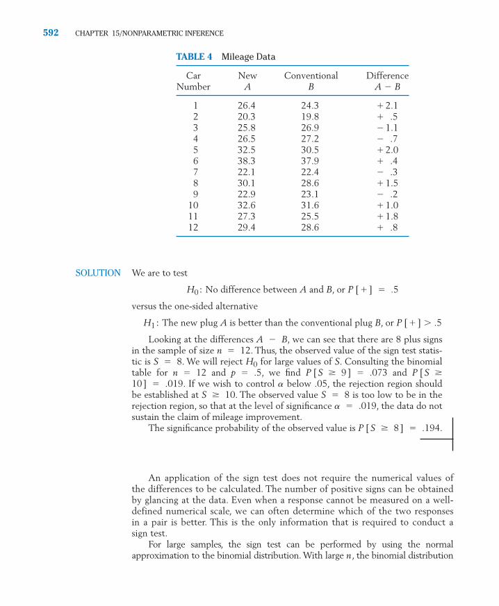
SOLUTION We are to test
� No difference between A and B, or P [�] � .5
versus the one-sided alternative
� The new plug A is better than the conventional plug B, or P [�] � .5
Looking at the differences A � B, we can see that there are 8 plus signsin the sample of size n � 12. Thus, the observed value of the sign test statis-tic is S � 8. We will reject for large values of S. Consulting the binomialtable for n � 12 and p � .5, we find P [S � 9] � .073 and P [S �10] � .019. If we wish to control a below .05, the rejection region shouldbe established at S � 10. The observed value S � 8 is too low to be in therejection region, so that at the level of significance a � .019, the data do notsustain the claim of mileage improvement.
The significance probability of the observed value is P [S � 8] � .194.
An application of the sign test does not require the numerical values ofthe differences to be calculated. The number of positive signs can be obtainedby glancing at the data. Even when a response cannot be measured on a well-defined numerical scale, we can often determine which of the two responsesin a pair is better. This is the only information that is required to conduct asign test.
For large samples, the sign test can be performed by using the normalapproximation to the binomial distribution. With large n , the binomial distribution
H0
H1
H0
592 CHAPTER 15/NONPARAMETRIC INFERENCE
TABLE 4 Mileage Data
Car New Conventional DifferenceNumber A B A � B
1 26.4 24.3 � 2.12 20.3 19.8 � .53 25.8 26.9 � 1.14 26.5 27.2 � .75 32.5 30.5 � 2.06 38.3 37.9 � .47 22.1 22.4 � .38 30.1 28.6 � 1.59 22.9 23.1 � .2
10 32.6 31.6 � 1.011 27.3 25.5 � 1.812 29.4 28.6 � .8
c15.qxd 10/15/09 11:37 AM Page 592

with p � .5 is close to the normal distribution with mean n/2 and standard deviation
Example 7 Applying the Sign Test to a Large Sample of Beer PreferencesIn a TV commercial filmed live, 100 persons tasted two beers A and B andeach selected their favorite. A total of S � 57 preferred beer A. Does thisprovide strong evidence that A is more popular?
SOLUTION According to the large sample approximation,
The significance probability P [ Z � 1.4 ] � .0808 is not small enough toprovide strong support to the claim that beer A is more popular.
HANDLING TIES
When the two responses in a pair are exactly equal, we say that there is a tie.Because a tied pair has zero difference, it does not have a positive or a negativesign. In the presence of ties, the sign test is performed by discarding the tiedpairs, thereby reducing the sample size. For instance, when a sample of n � 20pairs has 10 plus signs, 6 minus signs, and 4 ties, the sign test is performed withthe effective sample size n � 20 � 4 � 16 and S � 10.
THE WILCOXON SIGNED-RANK TEST
We have already noted that the sign test extends to ordinal data for which theresponses in a pair can be compared without being measured on a numericalscale. However, when numerical measurements are available, the sign test mayresult in a considerable loss of information because it includes only the signs ofthe differences and disregards their magnitudes. Compare the two sets of paireddifferences plotted in the dot diagrams in Figure 3. In both cases, there are n �6 data points with 4 positive signs, so that the sign test will lead to identical
Z �S � n / 2
√n / 4�
57 � 50
√ 25� 1.4
√ n / 4.
3. MATCHED PAIRS COMPARISONS 593
Large Sample Approximation to the Sign Test Statistic
Under ,
is approximately distributed as N (0, 1).
Z �S � n / 2
√ n / 4
H0
c15.qxd 10/15/09 11:37 AM Page 593

conclusions. However, the plot in Figure 3b exhibits more of a shift toward thepositive side, because the positive differences are farther away from zero thanthe negative differences. Instead of attaching equal weights to all the positivesigns, as is done in the sign test, we should attach larger weights to the plus signsthat are farther away from zero. This is precisely the concept underlying thesigned-rank test.
In the signed-rank test, the paired differences are ordered according totheir numerical values without regard to signs, and then the ranks associatedwith the positive observations are added to form the test statistic. To illustrate,we refer to the mileage data given in Example 6 where the paired differencesappear in the last column of Table 4. We attach ranks by arranging these differ-ences in increasing order of their absolute values and record the correspondingsigns.
Paireddifferences 2.1 .5 � 1.1 � .7 2.0 .4 � .3 1.5 � .2 1.0 1.8 .8
Orderedabsolutevalues .2 .3 .4 .5 .7 .8 1.0 1.1 1.5 1.8 2.0 2.1
Ranks 1 2 3 4 5 6 7 8 9 10 11 12Signs � � � � � � � � � � � �
The signed-rank statistic is then calculated as
If the null hypothesis of no difference in treatment effects is true, then thepaired differences , , . . . , constitute a random sample from a popu-lation that is symmetric about zero. On the other hand, the alternate hypothesisthat treatment A is better asserts that the distribution is shifted from zerotoward positive values. Under , not only are more plus signs anticipated, butthe positive signs are also likely to be associated with larger ranks. Consequently,
is expected to be large under the one-sided alternative, and we select a re-jection region in the upper tail of .T �T �
H1
DnD2D1
� 62 � 3 � 4 � 6 � 7 � 9 � 10 � 11 � 12
T� � sum of the ranks associated with positive observations
T�
594 CHAPTER 15/NONPARAMETRIC INFERENCE
+
0
–– + + +
(a)
+ +
0
–– + +
(b)
Figure 3 Two plots of paired differences with the same number of � signs but withdifferent locations for the distributions.
c15.qxd 10/15/09 11:37 AM Page 594

Selected tail probabilities of the null distribution of are given in Appen-dix B, Table 8 for n � 3 to n � 15.
USING APPENDIX B, TABLE 8
By symmetry of the distribution around n ( n � 1) /4, we obtain
when The x and x* values in Appendix B, Table 8satisfy this relation. To illustrate the use of this table, we refer once again to themileage data given in Example 6. There, n � 12 and the observed value of is found to be 62. From the table, we find P [ � 61 ] � .046. Thus, thenull hypothesis is rejected at the level of significance a � .046, and a signifi-cant mileage improvement using the new type of spark plug is indicated.
n � 12
P � P [ T� � x ] � P [ T� � x* ]
T �T �
x* � n ( n � 1 ) / 2 � x.
P [ T� � x ] � P [ T� � x* ]
T �
3. MATCHED PAIRS COMPARISONS 595
Steps in the Signed-Rank Test
1. Calculate the differences � � , i � 1, . . . , n .
2. Assign ranks by arranging the absolute values of the in increasingorder; also record the corresponding signs.
3. Calculate the signed-rank statistic � sum of ranks of positivedifferences .
4. Set the rejection region at the upper tail, lower tail, or at both tails of, according to whether treatment A is stated to have a higher,
lower, or different response than treatment B under the alternativehypothesis.
T�
Di
T �
Di
YiXiDi
x P x*
56 22
: 61 .046 1762 16
68 10
c15.qxd 10/15/09 11:37 AM Page 595

With increasing sample size n, the null distribution of is closelyapproximated by a normal curve, with mean n (n � 1) /4 and variancen (n � 1) (2n � 1) / 24.
This result can be used to perform the signed-rank test with large samples.
Example 8 Applying the Signed-rank Test to Compare Spark PlugsRefer to the mileage data in Example 6. Obtain the significance probabilityfor the signed-rank test using (a) the exact distribution in Appendix B, Table8 and (b) the large sample approximation.
SOLUTION (a) For the mileage data, � 62 and n � 12. From Appendix B,Table 8, the exact significance probability is P [ � 62 ] � .039.
(b) The normal approximation to this probability uses
From the normal table, we approximate by .036.
The normal approximation improves with increasing sample size.
*HANDLING TIES
In computing the signed-rank statistic, ties may occur in two ways: Some ofthe differences may be zero or some nonzero differences may have thesame absolute value. The first type of tie is handled by discarding the zero valuesafter ranking. The second type of tie is handled by assigning the average rank toeach observation in a group of tied observations with nonzero differences .
See Lehmann [1] for instructions on how to modify the critical values toadjust for ties.
Di
DiDi
P [ Z � 1.804 ] �P [ T� � 62 ]
z �62 � 12(13 ) / 4
√ 12( 13 ) ( 25 ) / 24�
2312.75
� 1.804
T�T �
T �
596 CHAPTER 15/NONPARAMETRIC INFERENCE
Large Sample Approximation to Signed-Rank Statistic
is approximately distributed as N(0, 1).
Z �T� � n ( n � 1 ) / 4
√ n ( n � 1 ) ( 2n � 1 ) / 24
c15.qxd 10/15/09 11:37 AM Page 596

Exercises
3. MATCHED PAIRS COMPARISONS 597
Service RatingRestaurant Critic 1 Critic 2
1 6.1 7.32 5.2 5.53 8.9 9.14 7.4 7.05 4.3 5.16 9.7 9.8
Answer ofCouple Husband Wife
1 3 22 1 13 2 14 2 35 5 16 0 17 0 28 1 39 2 2
10 3 111 4 212 1 213 3 314 2 115 3 2
Answer ofCouple Husband Wife
16 2 217 0 018 1 219 2 120 3 221 4 322 3 123 0 024 1 225 1 1
15.13 In a taste test of two chocolate chip cookierecipes, 13 out of 18 subjects favored recipe A.Using the sign test, find the significance proba-bility when states that recipe A is preferable.
15.14 Two critics rate the service at six award-winningrestaurants on a continuous 0-to-10 scale. Isthere a difference between the critics’ ratings?
(a) Use the sign test with a below .05.
(b) Find the significance probability.
15.15 A social researcher interviews 25 newlymarried couples. Each husband and wife areindependently asked the question: “How manychildren would you like to have?” The follow-ing data are obtained.
H1
Do the data show a significant difference of opin-ion between husbands and wives regarding anideal family size? Use the sign test with a closeto .05.
15.16 Use Appendix B, Table 8, to find:
(a) when n � 11.
(b) when n � 15.
(c) The value of c so that isnearly .05 when n � 14.
15.17 Use Appendix B, Table 8, to find:
(a) when n � 12.
(b) when n � 10.
(c) The value c such that when n � 8.
(d) The values and such that .027 when n �
11.
15.18 Referring to Exercise 15.14, apply theWilcoxon signed-rank test with a near .05.
15.19 The null distribution of the Wilcoxon signed-rank statistic is determined from the factthat under the null hypothesis of a sym-metric distribution about zero, each of theranks 1, 2, . . . , n is equally likely to beassociated with a positive sign or a negative
T �
c1 ] � P [ T� � c2
] �
P [ T� �c2c1
.039P [ T� � c ] �
P [ T� � 10 ]
P [ T� � 65 ]
P [ T� � c ]
P [ T� � 32 ]
P [ T� � 54 ]
c15.qxd 10/15/09 11:37 AM Page 597
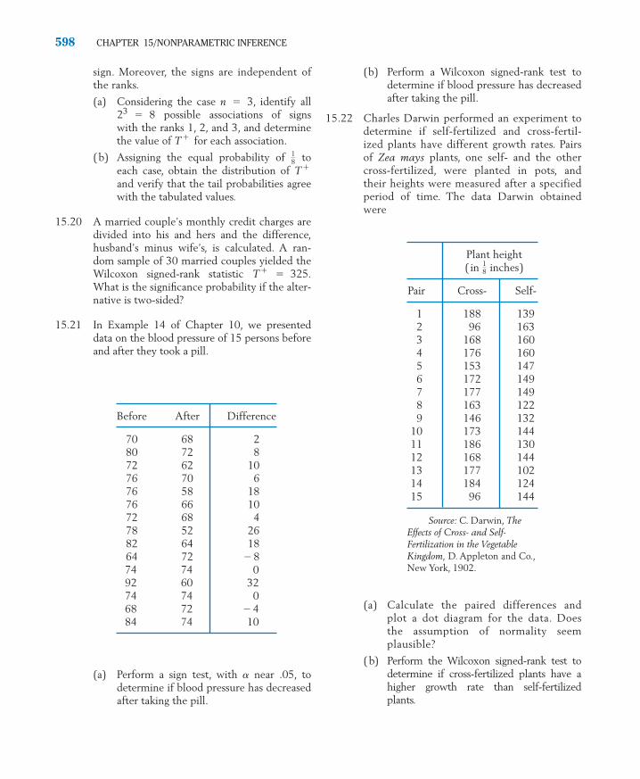
sign. Moreover, the signs are independent ofthe ranks.
(a) Considering the case n � 3, identify all� 8 possible associations of signs
with the ranks 1, 2, and 3, and determinethe value of for each association.
(b) Assigning the equal probability of toeach case, obtain the distribution of and verify that the tail probabilities agreewith the tabulated values.
15.20 A married couple’s monthly credit charges aredivided into his and hers and the difference,husband’s minus wife’s, is calculated. A ran-dom sample of 30 married couples yielded theWilcoxon signed-rank statistic � 325.What is the significance probability if the alter-native is two-sided?
15.21 In Example 14 of Chapter 10, we presenteddata on the blood pressure of 15 persons beforeand after they took a pill.
T�
T �
18
T �
23
598 CHAPTER 15/NONPARAMETRIC INFERENCE
Plant height( in inches)
Pair Cross- Self-
1 188 1392 96 1633 168 1604 176 1605 153 1476 172 1497 177 1498 163 1229 146 132
10 173 14411 186 13012 168 14413 177 10214 184 12415 96 144
18
Before After Difference
70 68 280 72 872 62 1076 70 676 58 1876 66 1072 68 478 52 2682 64 1864 72 � 874 74 092 60 3274 74 068 72 � 484 74 10
Source: C. Darwin, TheEffects of Cross- and Self-Fertilization in the VegetableKingdom, D. Appleton and Co.,New York, 1902.
(b) Perform a Wilcoxon signed-rank test todetermine if blood pressure has decreasedafter taking the pill.
15.22 Charles Darwin performed an experiment todetermine if self-fertilized and cross-fertil-ized plants have different growth rates. Pairsof Zea mays plants, one self- and the othercross-fertilized, were planted in pots, andtheir heights were measured after a specifiedperiod of time. The data Darwin obtainedwere
(a) Perform a sign test, with a near .05, todetermine if blood pressure has decreasedafter taking the pill.
(a) Calculate the paired differences andplot a dot diagram for the data. Doesthe assumption of normality seemplausible?
(b) Perform the Wilcoxon signed-rank test todetermine if cross-fertilized plants have ahigher growth rate than self-fertilizedplants.
c15.qxd 10/15/09 11:37 AM Page 598

4. MEASURE OF CORRELATION BASED ON RANKS
Ranks may also be employed to determine the degree of association betweentwo random variables. These two variables could be mathematical ability andmusical aptitude or the aggressiveness scores of first- and second-born sons on apsychological test. We encountered this same general problem in Chapter 3,where we introduced Pearson’s product moment correlation coefficient
as a measure of association between X and Y. Serving as a descriptive statistic,r provides a numerical value for the amount of linear dependence between Xand Y.
Before we present a measure of association, we note a few simplifying prop-erties. Because each of the ranks, 1, 2, . . . , n must occur exactly once in theset , , . . . , , it can be shown that
�n
i � 1 ( Ri � R )2 �
n ( n2 � 1 )12
R �1 � 2 � � n
n�
n � 12
RnR2R1
r �
�n
i � 1 ( Xi � X )( Yi � Y )
� �n
i � 1 ( Xi � X )2 � �
n
i � 1 ( Yi � Y )2
4. MEASURE OF CORRELATION BASED ON RANKS 599
Structure of the Observations
The n pairs ( , ), ( , ), . . . , ( , ) are independent, andeach pair has the same continuous bivariate distribution. The , . . . ,
are then ranked among themselves, and the , . . . , are rankedamong themselves:
Pair no. 1 2 n
Ranks of Ranks of SnS2S1Yi
RnR2R1Xi
YnY1Xn
X1
YnXnY2X2Y1X1
c15.qxd 10/15/09 11:37 AM Page 599

for all possible outcomes. Similarly,
A measure of correlation is defined by C. Spearman that is analogous toPearson’s correlation r, except that Spearman replaces the observations withtheir ranks. Spearman’s rank correlation is defined by
This rank correlation shares the properties of r that �1 � � 1 and thatvalues near �1 indicate a tendency for the larger values of X to be paired withthe larger values of Y. However, the rank correlation is more meaningful,because its interpretation does not require the relationship to be linear.
Example 9 Calculating Spearman’s Rank CorrelationAn interviewer in charge of hiring large numbers of data entry persons wishesto determine the strength of the relationship between ranks given on the basisof an interview and scores on an aptitude test. The data for six applicants are
5 2 3 1 6 4
47 32 29 28 56 38
Calculate .rSp
Aptitudescore
Interviewrank
rSp
rSp �
�n
i � 1 ( Ri � R )( Si � S )
� �n
i � 1 ( Ri � R )2 � �
n
i � 1 ( Si � S )2
�
�n
i � 1 �
Ri �n � 1
2 � � Si �
n � 12
�n ( n2 � 1 ) / 12
rSp
S �n � 1
2 and �
n
i � 1 ( Si � S )2 �
n( n2 � 1 )12
600 CHAPTER 15/NONPARAMETRIC INFERENCE
Spearman’s Rank Correlation
1. � 1 � � 1.
2. near �1 indicates a tendency for the larger values of X to be associ-ated with the larger values of Y. Values near �1 indicate the oppositerelationship.
3. The association need not be linear; only an increasing / decreasing re-lationship is required.
rSp
rSp
rSp �
�n
i � 1 � Ri �
n � 12
� � Si �n � 1
2 �
n ( n2 � 1 ) / 12
c15.qxd 10/15/09 11:37 AM Page 600

SOLUTION There are 6 ranks, so that and n ( � 1)/12 � 35/2 � 17.5. Ranking the aptitude scores, we obtain
Interview 5 2 3 1 6 4
Aptitude 5 3 2 1 6 4
Thus,
and
The relationship between interview rank and aptitude score appears tobe quite strong.
Figure 4 helps to stress the point that is a measure of any monotonerelationship, not merely a linear relation.
A large sample approximation to the distribution of is available.rSp
rSp
rSp �16.517.5
� .943
� 16.5
� 1.5(1.5) � (�1.5)(� .5) � � (.5)(.5)
� (5 � 3.5)( 5 � 3.5) � (2 � 3.5)(3 � 3.5) � � ( 4 � 3.5)(4 � 3.5)
�n
i � 1 �
Ri �n � 1
2 � � Si �
n � 12
�
Si
Ri
n2R � ( n � 1 ) / 2 � 7 / 2 � 3.5
4. MEASURE OF CORRELATION BASED ON RANKS 601
rSp = .99
r is inappropriate
Figure 4 is a measure of anymonotone relationship.
rSp
If X and Y are independent,
is approximately distributed as N(0, 1)
provided that the sample size is large.
rSp√ n � 1
c15.qxd 10/15/09 11:37 AM Page 601

This approximation leads to a convenient form of a test for independence.Reject
� X and Y are independent
in favor of
� Large values of X and Y tend to occur together and small values tend to occur together
if
Recall that is the upper a point of a standard normal distribution. Two-tailedtests can also be conducted.
Example 10 Establishing Dependence When Large X and YTend to Occur Together and so Do Small X and YThe grade point average (GPA) and Scholastic Achievement Test (SAT)scores for 40 applicants yielded � .4. Do large values of GPA and SAT tend to occur together? That is, test for lack of independence using a � .05.
SOLUTION For a � .05, the rejection region is Since
we reject : X and Y are independent at level a � .05. Large values ofGPA and SAT tend to occur together and so do small values.
Exercises
H0
√n � 1 rSp � √39(.4) � 2.498
√ n � 1 rSp � z.05 � 1.96.
rSp
z
√ n � 1 rSp � za
H1
H0
602 CHAPTER 15/NONPARAMETRIC INFERENCE
15.23 Refer to Exercise 11.31 and the first four coun-tries in Table 8. The number of Internet usersper one hundred residents and the human devel-opment index(HDI) are
Internet/100 21.3 26.2 14.3 20.6
HDI .866 .870 .852 .824
Calculate Spearmann’s rank correlation.
15.24 Refer to Exercise 11.68 and the height and speedof the four tallest roller coasters. Given the data
Height 456 420 415 377
Speed 128 120 100 107
Evaluate rSp
15.25 The following scores are obtained on a test ofdexterity and aggression administered to arandom sample of 10 high-school seniors.
Student 1 2 3 4 5 6 7 8 9 10
Dexterity 23 29 45 36 49 41 30 15 42 38
Aggression 45 48 16 28 38 21 36 18 31 37
Evaluate Spearman’s statistic.
15.26 Referring to Example 10, determine the signif-icance probability of � .4, using theone-sided test, when n � 40.
rSp
c15.qxd 10/15/09 11:37 AM Page 602

5. CONCLUDING REMARKS
In contrast to nonparametric procedures, Student’s t and the chi-square statis-tic were developed to make inferences about the parametersm and s of a normal population. These normal-theory parametric procedurescan be seriously affected when the sample size is small and the underlyingdistribution is not normal. Drastic departures from normality can occur inthe forms of conspicuous asymmetry, sharp peaks, or heavy tails. For instance,a t test with an intended level of significance of a � .05 may have an actualType I error probability far in excess of this value. These effects are mostpronounced for small or moderate samples sizes precisely when it is mostdifficult to assess the shape of the population. The selection of a parametricprocedure leaves the data analyst with the question: Does my normalityassumption make sense in the present situation? To avoid this risk, a nonpara-metric method could be used in which inferences rest on the safer ground ofdistribution-free properties.
When the data constitute measurements on a meaningful numerical scaleand the assumption of normality holds, parametric procedures are certainlymore efficient in the sense that tests have higher power than their nonpara-metric counterparts. This brings to mind the old adage, “You get what youpay for.” A willingness to assume more about the population form leads toimproved inference procedures. However, trying to get too much for yourmoney by assuming more about the population than is reasonable can lead tothe “purchase” of invalid conclusions. A choice between the parametric andnonparametric approach should be guided by a consideration of loss of effi-ciency and the degree of protection desired against possible violations of theassumptions.
Tests are judged by two criteria: control of the Type I error probability andthe power to detect alternatives. Nonparametric tests guarantee the desired con-trol of the Type I error probability a, whatever the form of the distribution.However, a parametric test established at a � .05 for a normal distributionmay suffer a much larger a when a departure from normality occurs. This isparticularly true with small sample sizes. To achieve universal protection,nonparametric tests, quite expectedly, must forfeit some power to detect alter-natives when normality actually prevails. As plausible as this argument sounds, itis rather surprising that the loss in power is often marginal with such simpleprocedures as the Wilcoxon rank-sum test and the signed-rank test.
Finally, the presence of dependence among the observations affects the use-fulness of nonparametric and parametric methods in much the same manner.When either method is used, the level of significance of the test may seriouslydiffer from the nominal value selected by the analyst.
Caution: When successive observations are dependent, nonparametrictest procedures lose their distribution-free property, and conclusionsdrawn from them can be seriously misleading.
( n � 1 )S
2 / �
2
5. CONCLUDING REMARKS 603
c15.qxd 10/15/09 11:37 AM Page 603

Reference
1. E. L. Lehmann, Nonparametrics: Statistical Methods Based on Ranks,Springer, 2007.
USING STATISTICS WISELY
1. A one-sample nonparametric test will provide valid inferences witha small sample size where it may not be possible to check theassumption of normality. Of course, the power of the rank test willgenerally be less than the normal theory paired t test when normalityholds.
2. When the two sample sizes are small, it is a good idea toconduct a two-sample Wilcoxon rank-sum test. If software is available,also obtain the corresponding confidence interval for the difference inlocation. These provide a baseline comparison for the result based onthe t distribution.
3. If the sample sizes are large enough so the dot diagrams reveal a differ-ence in both location and spread, the Wilcoxon rank-sum test is notappropriate.
4. Remember that nonparametric tests can produce invalid inferences ifthere is time dependence between the observations.
KEY IDEAS AND FORMULAS
Nonparametric tests obtain their distribution-free character because rank ordersof the observations do not depend on the shape of the population distribution.
The Wilcoxon rank-sum test, based on the test statistic
� sum of ranks of the observations from population A, among all
� observations
applies to the comparison of two populations. It uses the combined sample ranks.In the paired-sample situation, equality of treatments can be tested using
either the sign test based on the statistic
S � No. of positive differences
or the Wilcoxon signed-rank based on the statistic
� sum, over positive differences, of the ranks of their absolute values
The level of a nonparametric test holds whatever the form of the (continu-ous) population distribution.
Any tie in the observations requires specific handling.
T �
nBnA
nAWA
604 CHAPTER 15/NONPARAMETRIC INFERENCE
c15.qxd 10/15/09 11:37 AM Page 604

TECHNOLOGY
Nonparametric tests and confidence intervals
MINITAB
One sample—inference about median
Start with the data in C1. To find a 95% confidence interval for the medianusing the sign test:
Stat Q Nonparametrics Q 1-Sample Sign.Type C1 in Variables. Click Confidence interval and type 0.95 in Level.Click OK.
To test a hypothesis concerning the median, instead of Confidence interval:
Click Test Median and choose the form of the Alternative hypothesis. Youcannot set the level.
To find a 95% confidence interval for the median using the Wilcoxonsigned-rank test:
Stat Q Nonparametrics Q 1-Sample Wilcoxon.Type C1 in Variables. Click Confidence interval and type 0.95 in Level.Click OK.
To test a hypothesis concerning the median, instead of Confidence interval:
Click Test Median and choose the form of the Alternative hypothesis.
Two-sample Wilcoxon test for equality of populations
Start with the data from the first population in C1 and the data from thesecond in C2. To test at level a � .05:
Stat Q Nonparametrics Q Mann-Whitney.Type C1 and C2 in Variables. Type 0.95 in Confidence level and select theform of the Alternative. Click OK.
The output includes a confidence interval for the difference in locations.
6. REVIEW EXERCISES
6. REVIEW EXERCISES 605
15.27 From the campus crime statistics in Chapter 11,Table 5, the number of burglaries at the threeuniversities in Florida, population A, and thethree in California are
15.28 Using Appendix B, Table 7, find:
(a) when � 5, � 7.(b) when � 6, � 6.(c) when �
10, � 7.(d) The point c such that P [ WS � c] � .036
when � 8, � 4.n2n1
n2
n1P [ WS � 81 or WS � 45 ]n2n1P [ WS � 25 ]n2n1P [ WS � 42 ]
Florida 43 69 90
California 61 74 42
Evaluate WA (continued)
c15.qxd 10/16/09 2:26 PM Page 605

(e) The points and such that P [ �] � P [ � c1] � .05 when � 3,
� 9.
15.29 (a) Evaluate all possible rank configurationsassociated with treatment A when � 3and � 2.
(b) Determine the null distribution of .
15.30 Five finalists in a figure-skating contest are ratedby two judges on a 10-point scale as follows:
WA
nB
nA
n2
n1WSc2
WSc2c1
Calculate the Spearman’s rank correlationbetween the two ratings.
15.31 Using Appendix B, Table 8, find:
(a) when n � 8.
(b) when n � 9.(c) The point c such that is
approximately .05 when n � 13.
15.32 Referring to Exercise 15.30, calculate:
(a) The sign test statistic.
(b) The significance probability when thealternative is that Judge 2 gives higherscores than Judge 1.
15.33 In a study of the cognitive capacities of non-human primates, 19 monkeys of the same ageare randomly divided into two groups of 10and 9. The groups are trained by two differ-ent teaching methods to recollect an acousticstimulus. The monkeys’ scores on a subse-quent test are seen below.Do the data strongly indicate a difference inthe recollection abilities of monkeys trainedby the two methods? Use the Wilcoxon rank-sum test with a close to .10.
P [ T� � c ]P [ T� � 5 ]
P [ T� � 28 ]
rSp
15.34 A mixture of compounds called phenolicsoccurs in wood waste products. It has beenfound that when phenolics are present inlarge quantities, the waste becomes unsuit-able for use as a livestock feed. To comparetwo species of wood, a dairy scientist mea-sures the percentage content of phenolicsfrom 6 batches of waste of species A and 7batches of waste of species B. The followingdata are obtained.
606 CHAPTER 15/NONPARAMETRIC INFERENCE
Contestants A B C D E
Judge 1 6 9 2 8 5Judge 2 8 10 4 7 3
Memory Scores
Method 1 167 149 137 178 179 155 164 104 151 150
Method 2 98 127 140 103 116 105 100 95 131
Percentage of Phenolics
Species A 2.38 4.19 1.39 3.73 2.86 1.21
Species B 4.67 5.38 3.89 4.67 3.58 4.96 3.98
Use the Wilcoxon rank-sum test to determine ifthe phenolics content of species B is signifi-cantly higher than that of species A. Use a
close to .05.
15.35 (a) Calculate Spearman’s rank correlation forthe data on Chester Whites in Exercise15.6.
(b) Test for independence of calcium andphosphate levels using the rejection region
(c) What is the approximate level of signifi-cance?
15.36 In the study described in Exercise 1.5, golferswere asked to estimate the size of the hole (cm)in the green by selecting among nine in aboard. The size selected and their score for theday for three golfers are
√ n � 1 rSp � 1.96 or � �1.96
Hole size 11.5 10.0 10.5
Score 84 104 94
Evaluate .rSp
c15.qxd 10/15/09 11:37 AM Page 606

15.37 Refer to Exercise 10.76. Evaluate:
(a) Sign test statistic.
(b) Signed-rank statistic.
*15.38 Confidence interval for median using the signtest. Let , . . . , be a random samplefrom a continuous population whose medianis denoted by M. For testing � M � ,we can use the sign test statistic S � No. of
� , i � 1, . . . , n. is rejected atlevel a in favor of �M � if S � r or S � n � r � 1, where r is the largest inte-ger satisfying
�r
x � 0 b ( x ; n, .5 ) � / 2
M0H1
H0M0Xi
M0H0
XnX1
If we repeat this test procedure for all possiblevalues of , a 100 ( 1 � a ) % confidenceinterval for M is then the range of values so that S is in the acceptance region. Orderingthe observations from smallest to largest, verifythat this confidence interval becomes
( r � 1)st smallest to ( r � 1)st largest observation
(a) Refer to Example 6. Using the sign test,construct a confidence interval for the pop-ulation median of the differences A � B,with a level of confidence close to 95%.
(b) Repeat part (a) using Darwin’s data givenin Exercise 15.22.
M0
M0
6. REVIEW EXERCISES 607
c15.qxd 10/15/09 11:37 AM Page 607

c15.qxd 10/15/09 11:37 AM Page 608

A1APPENDIX
Summation Notation
A1.1 SUMMATION AND ITS PROPERTIES
The addition of numbers is basic to our study of statistics. To avoid a detailedand repeated writing of this operation, the symbol � (the Greek capital lettersigma) is used as mathematical shorthand for the operation of addition.
Summation Notation �
The notation represents the sum of n numbers , , . . . , and
is read as the sum of all with i ranging from 1 to n.
�n
i � 1 xi � x1 � x2 � � � � � xn
xi
xnx2x1�n
i � 1 xi
The term following the sign � indicates the quantities that are beingsummed, and the notations on the bottom and the top of the � specify therange of the terms being added. For instance,
�4
i � 1 ( xi � 3) � ( x1 � 3) � ( x2 � 3) � ( x3 � 3) � ( x4 � 3)
�3
i � 1 xi � x1 � x2 � x3
bapp01.qxd 10/15/09 11:52 AM Page 609

610 APPENDIX A1/SUMMATION NOTATION
Example Suppose that the four measurements in a data set are given as Compute the numerical values of
(a) (b) (c)
(d) (e) (f )
SOLUTION (a)
( b)
(c)
(d)
(e)
(f )
Alternatively, noting that we can write
� 54 � 6 ( 14 ) � 36 � 6
� �4
i � 1 x2
i � 6 � �4
i � 1 xi� � 4(9)
�( x23 � 6x3 � 9)�( x2
4 � 6x4 � 9)
� ( x21 � 6x1 � 9) � ( x2
2 � 6x2 � 9)
�4
i � 1 ( xi � 3 )2 � �
4
i � 1 ( x2
i � 6xi � 9 )
( xi � 3 )2 � x2i � 6xi � 9,
� 1 � 4 � 0 � 1 � 6
� ( 3 � 3 )2 � ( 4 � 3 )2
� ( 2 � 3 )2 � ( 5 � 3 )2� ( x3 � 3 )2 � ( x4 � 3 )2
�4
i � 1 ( xi � 3)2 � ( x1 � 3)2 � ( x2 � 3)2
�4
i � 1 x2
i � x21 � x2
2 � x23 � x2
4 � 22 � 52 � 32 � 42 � 54
� �4
i � 1 xi � 4 ( 3 ) � 14 � 12 � 2
� ( x3 � 3) � ( x4 � 3)
�4
i � 1 ( xi � 3 ) � ( x1 � 3 ) � ( x2 � 3 )
� 2 � 14 � 28
�4
i � 1 2xi � 2x1 � 2x2 � 2x3 � 2x4 � 2 � �
4
i � 1 xi�
�4
i � 1 6 � 6 � 6 � 6 � 6 � 4 ( 6 ) � 24
�4
i � 1 xi � x1 � x2 � x3 � x4 � 2 � 5 � 3 � 4 � 14
�4
i � 1 ( xi � 3 )2�
4
i � 1 x2
i�4
i � 1 ( xi � 3)
�4
i � 1 2xi�
4
i � 1 6�
4
i � 1 xi
x4 � 4.x3 � 3,x2 � 5,x1 � 2,
bapp01.qxd 10/15/09 11:52 AM Page 610

A1.2 SOME BASIC USES OF � IN STATISTICS 611
Some Basic Properties of Summation
If a and b are fixed numbers,
�n
i � 1 ( xi � a)2 � �
n
i � 1 x2
i � 2a �n
i � 1 xi � na2
�n
i � 1 ( b xi � a) � b �
n
i � 1 xi � na
�n
i � 1 b xi � b �
n
i � 1 xi
Exercises
1. Demonstrate your familiarity with the summation notation by evaluatingthe following expressions when
(a) (b) (c)
(d) (e) (f )
(g) (h) (i)
2. Five measurements in a data set are Determine
(a) (b) (c)
(d) (e) (f )
A1.2 SOME BASIC USES OF � IN STATISTICS
Let us use the summation notation and its properties to verify some computa-tional facts about the sample mean and variance.
�4
i � 1 ( xi � 5)2�
5
i � 1 ( xi � 6)2�
5
i � 1 ( xi � 6)
�5
i � 1 2�
3
i � 2 xi�
5
i � 1 xi
x5 � 7.x4 � 5,x3 � 6,x2 � 3,x1 � 4,
�3
i � 1 ( x2
i � 6 xi � 9)�3
i � 1 ( xi � 3)2�
3
i � 1 x2
i
�3
i � 1 ( xi � 2)2�
3
i � 1 ( xi � 3)�
3
i � 1 ( xi � 2)
�3
i � 1 5xi�
3
i � 1 7�
3
i � 1 xi
x1 � 4, x2 � �2, x3 � 1.
A few basic properties of the summation operation are apparent from thenumerical demonstration in the example.
bapp01.qxd 10/15/09 11:52 AM Page 611

� ( � ) � 0
The total of the deviations about the sample mean is always zero. Since we can write
Consequently, whatever the observations,
We could also verify this directly with the second property for summation inA1.1, when and
ALTERNATIVE FORMULA FOR
By the quadratic rule of algebra,
Therefore,
Using in place of we get
We could also verify this directly from the third property for summation, inA1.1, with
This result establishes that
so the two forms of are equivalent.s2
s2 �
�n
i � 1 ( xi � x )2
n � 1�
� x2i � ( � xi
)2 / nn � 1
a � x.
� � x2i �
( � xi )2
n
� � x2i �
2 ( � xi )2
n�
( � xi )2
n
� ( xi � x )2 � � x2i �
2 ( � xi )2
n�
n ( � xi )2
n2
x,(� xi) / n
� � x2i � 2x � xi � nx2
� ( xi � x )2 � � x2
i � � 2x xi � � x2
( xi � x )2 � x2i � 2 x xi � x2
s2
a � �x.b � 1
� n x � n x � 0
� x1 � x2 � � � � � xn � nx
�n
i � 1 ( xi � x ) � ( x1 � x ) � ( x2 � x ) � � � � � ( xn � x )
�n
i � 1 xi � x1 � x2 � � � � � xn � n x
(x1 � x2 � � � � � xn) / n,x �
xxi
612 APPENDIX A1/SUMMATION NOTATION
bapp01.qxd 10/15/09 11:52 AM Page 612

SAMPLE CORRELATION COEFFICIENT
The sample correlation coefficient and slope of the fitted regression line containa term
which is a sum of the products of the deviations. To obtain the alternative form,first note that
We treat xi yi as a single number, with index i, and conclude that
Since and
Consequently, either or canbe used for the calculation of with similar choices for and .SyySxxSxy
� xi yi � ( � xi ) ( � yi
) / n� ( xi � x ) ( yi � y )
� � xi yi �( � xi
) ( � yi )
n
�n ( � xi
)
n ( � yi
)
n
� ( xi � x )( yi � y ) � � xi yi �
( � yi )
n � xi �
( � xi )
n � yi
y � (� yi) / n,x � ( � xi ) / n
� � xi yi � y � xi � x � yi � n x y
� ( xi � x ) ( yi � y ) � � xi yi � � xi y � � xyi � � x y
( xi � x ) ( yi � y ) � xi yi � xi y � x yi � x y
Sxy � �n
i � 1 ( xi � x ) ( yi � y )
A1.2 SOME BASIC USES OF � IN STATISTICS 613
bapp01.qxd 10/15/09 11:52 AM Page 613

Some basic rules for counting can help us calculate probabilities. We begin withan example. Brazil (B ), United States (U.S.), Mexico (M), Canada (C), andJapan (J) are in the final round of a volleyball tournament. How many ways cana winner and second place finisher be selected?
To systematically address this problem, we create a tree diagram where thepossibilities for first place are represented by the initial 5 branches. For eachchoice of a first place finisher, there are four choices for second place. These arerepresented by the sets of 4 branches in the second stage. For instance, the left-most branch of the tree diagram depicts the case where Brazil is first and theUnited States second and so on.
US M C J B
B US M C J
M C J B US C J B US M J B US M C
A2APPENDIX
Rules for Counting
bapp02.qxd 10/15/09 11:53 AM Page 614

APPENDIX A2/RULES FOR COUNTING 615
Product Rule
An experiment consists of two parts where the first part has k distinctpossible outcomes and, for each outcome of the first part, there are m dis-tinct possible outcomes for the second part. Then, there are dis-tinct possible outcomes to the experiment.
k � m
The product rule is readily extended to experiments with more than twoparts. Suppose we are interested in the winner, second, and third place finishers inthe volleyball tournament. As above, by the product rule, there are distinct possibilities for selecting a first and second place volleyball team. Again,by the product rule, each of these 20 outcomes must be paired with one of the 3outcomes for a third place finisher so there are possibilities for the first, second, and third place finishers.
The term permutation means an ordering or arrangement of objects. Thenumber of different orderings or arrangements that can be formed with r ob-jects selected from a group of n distinct objects is called the number of permu-tations of r out of n and is denoted by
In the volleyball example, for the first two places andfor the first three places. When r objects are se-
lected, the first has n possibilities and the last possibilities.n � r � 1P5
3 � 5 � 4 � 3 � 60P 5
2 � 5 � 4 � 20P n
r .
20 � 3 � 5 � 4 � 3 � 60
5 � 4 � 20
There are terminal points or ways for these teams to finishfirst and second. Generalizing the tree diagram to k choices followed by mchoices, we obtain the product rule for counting.
5 � 4 � 20
Rule of Permutations or Arrangements
The number of different arrangements of r objects selected from agroup of n distinct objects is denoted by
Pnr � n ( n � 1 ) � � �( n � r � 1 )
P nr ,
If all n distinct objects are arranged in order, the number of possiblearrangements is which is the product ntimes on down through This special product, of decreasing in-tegers starting with n, is called n factorial and is denoted by n! .
When order is not important, we speak about collections of objects. Thenumber of different collections of r objects selected from a group of n distinctobjects is called the number of combinations of r out of n.
2 � 1.n � 1Pn
n � n ( n � 1 ) � � � � � 2 � 1,
bapp02.qxd 10/15/09 11:53 AM Page 615

616 APPENDIX A2/RULES FOR COUNTING
Rule of Combinations
The number of combinations, or different collections, of r objects selected
from a group of n distinct objects is denoted by
�nr � �
Pnr
r !�
n ( n � 1 ) � � �( n � r � 1 )r !
�n!
r ! ( n � r )!
�nr �,
The general formula for combinations is obtained by the following corre-spondence and an application of the product rule.
� � r !
According to the last form, is symmetric in r and Selecting r
objects to be in the collection is the same as choosing which to exclude.If 2 of the 5 volleyball teams must be selected to play another match, so the
order of selection is not important, there are 10 ways to select 2 to play or the 3teams which will not play.
�52� �
5 � 42 � 1
� 10 �5 � 4 � 3 � 2 � 1
2 � 1 � ( 3 � 2 � 1 )�
5 � 4 � 33 � 2 � 1
which equals �53�
n � r
n � r.�nr �
�nr �Pn
r
� Arrange r objectsselected from n � is the
same as � first select r
objects from n � andthen
� arrange the rselected objects �
bapp02.qxd 10/15/09 11:53 AM Page 616

A3APPENDIX
Expectation and Standard Deviation — Properties
The expected value of a discrete random variable is a summation of the prod-ucts (value � probability). The key properties of expectations are then all inher-ited from the properties of summation. In this appendix, we indicate this devel-opment for some of the most useful properties of expectation and variance. Theinterested reader can consult Bhattacharyya and Johnson1 for more details.
A3.1 EXPECTED VALUE AND STANDARD DEVIATION OF c X � b
The units of the random variable X may be changed by multiplying by a con-stant, for example,
or by adding a constant, for example,
X � 32 � degrees above freezing ( °F )
X � temperature ( °F )
X � height in feet, 12X � height in inches
1G. K. Bhattacharyya and Richard A. Johnson, Statistical Concepts and Methods, John Wiley &Sons, New York, 1978.
bapp03.qxd 10/15/09 11:54 AM Page 617

Finally, has mean and so hasmean � � 0 and
Any random variable having and can be con-verted to a
Var ( X ) � �2E ( X ) � �
sd � 15 (5) � 1.1
5 (0)
15 (X � 3)sd � 5,3 � 3 � 0(X � 3)
618 APPENDIX A3/EXPECTATION AND STANDARD DEVIATION—PROPERTIES
Random Variable Mean sd
cX cm �c �s
If a constant b is added to X,
Random Variable Mean sd
� (unchanged)� � bX � b
Notice that adding a constant to a random variable leaves the standard deviationunchanged.
Example Let X have mean � 3 � m and standard deviation � 5 � s. Find the meanand sd of (a) X � 4, ( b) 2X, (c) � X, and (d) (X � 3).
SOLUTION By the foregoing properties,
15
Random Variable Mean sd
52X
� �1 � 5 � 5(�1)3 � �3�X � (�1)X2(5) � 102(3) � 6
3 � 4 � 7X � 4
The mean and standard deviation of the new random variables are related toand
If X is multiplied by a constant c,� � sd ( X ).� � E ( X )
bapp03.qxd 10/15/09 11:54 AM Page 618

A3.2 ALTERNATIVE FORMULA FOR 619�2
Standardized variable
The standardized variable Z has mean � 0 and variance � 1. This was
checked for in the example above.
*VERIFICATION OF THE MEAN AND sd EXPRESSIONS FOR cX � b
Consider the random variable which includes the two cases above.The choice gives cX and the choice gives We restrictour verification to discrete random variables, where probability is attachedto . Because takes value with probability ,
and
Next,
so
Taking the positive square root yields Finally, taking and we obtain
so the standardized variable Z has
A3.2 ALTERNATIVE FORMULA FOR
An alternative formula for often simplifies the numerical calculations. Bydefinition,
�2 � � (deviation)2(probability) � � ( xi � �)2 f ( xi)
�2
�2
sd c � �1�
� � 1
mean c� � b �1�
� ��
�� 0
cX � b �1�
X ��
��
X � �
�� Z
b � �� / �,c � 1/�sd ( cX � b ) � � c ��.
� c2 � ( xi � � )2 f ( xi ) � c2�2
� � c2 ( xi � � )2 f ( xi )
variance � � (deviation)2 � probability
� ( cX � b ) � ( c� � b ) � cX � c� � c (X � � )
deviation � (random variable) � (mean)
� c � xi f (xi) � b � f (xi) � c� � b � 1
� � c xi f (xi) � � b f (xi)
mean � � (value � probability)
(value � probability) � ( c xi � b ) f (xi) � c xi f (xi) � b f (xi)
f (xi)c xi � bcX � bxi
f (xi)X � b.c � 1b � 0
cX � b,
Z �X � 3
5
Z �X � �
�
bapp03.qxd 10/15/09 11:54 AM Page 619

but can also be expressed as
To deduce the second form, we first expand the square of the deviation:
Then, multiply each term on the right-hand side by and sum:
First term
Second term � 2 since
Third term � � since � 1
Result:
Example Calculate by both formulas.
SOLUTION
�2
�2 � � x2i f (xi) � �2
� f (xi)�2�2 � f (xi)� xi f (xi) � ��2�2� � xi f (xi) �
� � x2i f ( xi)
f (xi)
(xi � �)2 � x2i � 2� xi � �2
�2 � � x2i f(xi) � �2
�2
620 APPENDIX A3/EXPECTATION AND STANDARD DEVIATION—PROPERTIES
Calculation
x f (x) x f (x)
1 .4 .4 1 .42 .3 .6 0 03 .2 .6 1 .24 .1 4
1.0 � �22.0 � �.4.4
( x � 2)2f ( x )(x � 2)2
� ( x � � )2 f ( x ) Calculation
x f (x) x f (x)
1 .4 .4 .42 .3 .6 1.23 .2 .6 1.84 .1
5.0
�2 � 5 � 22 � 1
2.0 � �1.6.4
x2 f (x)
� x2 f (x) � �2
A3.3 PROPERTIES OF EXPECTED VALUE FOR TWO RANDOM VARIABLES
The concept of expectation extends to two or more variables. With two randomvariables:
1. (additivity or sum law of expectation).
2. If X and Y are independent, then
Remark: Property 1 holds quite generally, independence is not required.
*DEMONSTRATION
We verify both (1) and (2) assuming independence. Independence implies thatfor all outcomes (x, y). ThatP [ X � x, Y � y ] � P [ X � x ] P [ Y � y ]
E( X Y ) � E(X ) E(Y ).
E( X � Y ) � E( X ) � E( Y )
bapp03.qxd 10/15/09 11:54 AM Page 620

is, the distribution of probability over the pairs of possible values (x, y) is speci-fied by the product
The expected value, is obtained by multiplying each possiblevalue by the probability and summing
� 1 � 1
Next,
�
Under the proviso that the random variables are independent, variancesalso add.
3. If X and Y are independent,
*DEMONSTRATION
We set and so by property 1,
Then, since variance is the expected value of ( variable � mean)2,
This last step follows since
�� E (X )E(Y ) � �1 �2 � �1
�2 � �1 �2 � 0 by property 2
� E(X Y ) � �1 �2
� E(X Y ) � �1E(Y ) � �2E(X ) � �1 �2
E( X � �1 )( Y � �2) � E(X Y � �1Y � X �2 � �1�2
)
� Var(X ) � Var(Y )
(by the sum law of expectation, property 1)
� E( X � �1 )2 � E ( Y � �2
)2 � 2E ( X � �1 ) ( Y � �2
)
� E[ ( X � �1 )2 � (Y � �2
)2 � 2 ( X � �1) ( Y � �2 ) ]
Var(X � Y ) � E(X � Y � �1 � �2)2
E(X � Y ) � �1 � �2
�2 � E(Y ),�1 � E(X )
Var (X � Y ) � Var(X ) � Var(Y )
� �x
x fX(x) ��y
y fY(y)� � E (X ) E (Y )
E ( X Y ) � �x
�y
x y fX (x) fY
(y)
� E(X ) � E (Y )
� ��x
x fX (x)� ��
y fY
(y)� � ��x
fX (x)� ��
y y fY
(y)� � �
x �
y x fX
(x) fY(y) � �x
�y
y fX(x) fY(y)
E (X � Y ) � �x
�y
( x � y ) fX (x) fY
(y)
fX ( x ) fY
( y )(x � y)E ( X � Y ),
fX (x) fY (y) � P [X � x, Y � y ].
A3.3 PROPERTIES OF EXPECTED VALUE FOR TWO RANDOM VARIABLES 621
� �
bapp03.qxd 10/15/09 11:54 AM Page 621

Some basic properties of the sampling distribution of can be expressed interms of the population mean and variance when the observations form a ran-dom sample. Let
In a random sample, the random variables , . . . , are independent, andeach has the distribution of the population. Consequently, each observation hasmean m and variance , or
Next,
and n is a constant. Using the additivity properties of expectation and variancediscussed in Appendix A3, we obtain
X �1n
( X1 � � � � � Xn)
Var ( X1) � � � � � Var ( Xn ) � �2 E ( X1) � � � � � E ( Xn ) � �
�2
XnX1
�2 � population variance
� � population mean
X
A4APPENDIX
The Expected Value and Standard Deviation of X
bapp04.qxd 10/15/09 11:54 AM Page 622

Furthermore, taking the square root yields
sd ( X ) � √Var(X) ��
√n
�1
n2 [ �2 � � � � � �2 ] �n�2
n2 ��2
n
�1
n2 [ Var ( X1) � � � � � Var ( Xn ) ] (variances add due to independence)
Var(X ) �1
n2 Var ( X1 � � � � � Xn )
�1n
[ � � � � � � � ] �n�
n� �
�1n
[ E (X1) � � � � � E(Xn) ] (mean of sum � sum of means)
E ( X ) �1n
E( X1 � � � � � Xn )
APPENDIX A4/THE EXPECTED VALUE AND STANDARD DEVIATION OF 623X
bapp04.qxd 10/15/09 11:54 AM Page 623

TABLE 1 Random Digits
Row
1 0695 7741 8254 4297 0000 5277 6563 9265 1023 59252 0437 5434 8503 3928 6979 9393 8936 9088 5744 47903 6242 2998 0205 5469 3365 7950 7256 3716 8385 02534 7090 4074 1257 7175 3310 0712 4748 4226 0604 38045 0683 6999 4828 7888 0087 9288 7855 2678 3315 6718
6 7013 4300 3768 2572 6473 2411 6285 0069 5422 61757 8808 2786 5369 9571 3412 2465 6419 3990 0294 08968 9876 3602 5812 0124 1997 6445 3176 2682 1259 17289 1873 1065 8976 1295 9434 3178 0602 0732 6616 7972
10 2581 3075 4622 2974 7069 5605 0420 2949 4387 7679
11 3785 6401 0540 5077 7132 4135 4646 3834 6753 159312 8626 4017 1544 4202 8986 1432 2810 2418 8052 271013 6253 0726 9483 6753 4732 2284 0421 3010 7885 843614 0113 4546 2212 9829 2351 1370 2707 3329 6574 700215 4646 6474 9983 8738 1603 8671 0489 9588 3309 5860
16 7873 7343 4432 2866 7973 3765 2888 5154 2250 433917 3756 9204 2590 6577 2409 8234 8656 2336 7948 747818 2673 7115 5526 0747 3952 6804 3671 7486 3024 985819 0187 7045 2711 0349 7734 4396 0988 4887 7682 899020 7976 3862 8323 5997 6904 4977 1056 6638 6398 4552
BAPPENDIX
Tables
bapp05.qxd 10/15/09 11:55 AM Page 624

APPENDIX B TABLES 625
TABLE 1 (Continued)
Row
21 5605 1819 8926 9557 2905 0802 7749 0845 1710 412522 2225 5556 2545 7480 8804 4161 0084 0787 2561 511323 2549 4166 1609 7570 4223 0032 4236 0169 4673 803424 6113 1312 5777 7058 2413 3932 5144 5998 7183 521025 2028 2537 9819 9215 9327 6640 5986 7935 2750 2981
26 7818 3655 5771 4026 5757 3171 6435 2990 1860 179627 9629 3383 1931 2631 5903 9372 1307 4061 5443 866328 6657 5967 3277 7141 3628 2588 9320 1972 7683 754429 4344 7388 2978 3945 0471 4882 1619 0093 2282 702430 3145 8720 2131 1614 1575 5239 0766 0404 4873 7986
31 1848 4094 9168 0903 6451 2823 7566 6644 1157 888932 0915 5578 0822 5887 5354 3632 4617 6016 8989 948233 1430 4755 7551 9019 8233 9625 6361 2589 2496 726834 3473 7966 7249 0555 6307 9524 4888 4939 1641 157335 3312 0773 6296 1348 5483 5824 3353 4587 1019 9677
36 6255 4204 5890 9273 0634 9992 3834 2283 1202 484937 0562 2546 8559 0480 9379 9282 8257 3054 4272 931138 1957 6783 4105 8976 8035 0883 8971 0017 6476 289539 7333 1083 0398 8841 0017 4135 4043 8157 4672 242440 4601 8908 1781 4287 2681 6223 0814 4477 3798 4437
41 2628 2233 0708 0900 1698 2818 3931 6930 9273 674942 5318 8865 6057 8422 6992 9697 0508 3370 5522 925043 6335 0852 8657 8374 0311 6012 9477 0112 8976 331244 0301 8333 0327 0467 6186 1770 4099 9588 5382 895845 1719 9775 1566 7020 4535 2850 0207 4792 6405 1472
46 8907 8226 4249 6340 9062 3572 7655 6707 3685 128247 6129 5927 3731 1125 0081 1241 2772 6458 9157 454348 7376 3150 8985 8318 8003 6106 4952 8492 2804 386749 9093 3407 4127 9258 3687 5631 5102 1546 2659 083150 1133 3086 9380 5431 8647 0910 6948 2257 0946 1245
51 4567 0910 8495 2410 1088 7067 8505 9083 4339 244052 6141 8380 2302 4608 7209 5738 9765 3435 9657 606153 1514 8309 8743 3096 0682 7902 8204 7508 8330 168154 7277 1634 7866 9883 0916 6363 5391 6184 8040 313555 4568 4758 0166 1509 2105 0976 0269 0278 7443 2431
56 9200 7599 7754 4534 4532 3102 6831 2387 4147 245557 3971 8149 4431 2345 6436 0627 0410 1348 6599 129658 2672 9661 2359 8477 3425 8150 6918 8883 1518 470859 1524 3268 3798 3360 2255 0371 7610 9114 9466 090160 6817 9007 5959 0767 1166 7317 7502 0274 6340 0427
bapp05.qxd 10/15/09 11:55 AM Page 625

626 APPENDIX B/TABLES
TABLE 1 (Continued)
Row
61 6762 3502 9559 4279 9271 9595 3053 4918 7503 516962 5264 0075 6655 4563 7112 7264 3240 2150 8180 136163 5070 8428 5149 2137 8728 9110 2334 9709 8134 392564 1664 3379 5273 9367 6950 6828 1711 7082 4783 014765 6962 7141 1904 6648 7328 2901 6396 9949 6274 1672
66 7541 4289 4970 2922 6670 8540 9053 3219 8881 189767 5244 4651 2934 6700 8869 0926 4191 1364 0926 287468 2939 3890 0745 2577 7931 3913 7877 2837 2500 877469 4266 6207 8083 6564 5336 5303 7503 6627 6055 360670 7848 5477 5588 3490 0294 3609 1632 5684 1719 6162
71 3009 1879 0440 7916 6643 9723 5933 0574 2480 689372 9865 7813 7468 8493 3293 1071 7183 9462 2363 652973 1196 1251 2368 1262 5769 9450 7485 4039 4985 661274 1067 3716 8897 1970 8799 5718 4792 7292 4589 455475 5160 5563 6527 7861 3477 6735 7748 4913 6370 2258
76 4560 0094 8284 7604 1667 9286 2228 9507 1838 464677 7697 2151 4860 0739 4370 3992 8121 2502 7670 447078 8675 2997 9783 7306 4116 6432 7233 4611 7121 941279 3597 3520 5995 0892 3470 4581 1068 8801 1254 860780 4281 8802 5880 6212 6818 8162 0052 1755 7107 5197
81 0101 0907 9057 2263 0059 8553 7855 7758 1020 126482 8179 0109 4412 6044 7167 4209 5250 4570 1984 827683 8980 9662 9333 6598 2990 8173 1753 1135 1409 204284 3050 2450 9252 6724 2697 7933 9540 3700 6561 279085 4465 1307 8782 6763 9202 5594 7166 7050 4462 0426
86 1925 5402 1379 3556 5109 4846 9827 2881 5574 902787 8753 4602 1838 4624 4632 2512 2652 4804 1624 511688 2645 9197 4541 4822 7883 3352 3202 0906 3676 814189 4287 5473 4493 7086 4271 9140 3315 7073 4533 065390 5280 5426 7240 2154 7952 3804 8097 9328 8069 6894
91 9553 3136 2112 1369 5562 7360 5530 8074 6488 368292 2975 7924 0253 3503 9383 9454 3320 3234 9255 352793 2596 7274 8967 8138 6868 0385 4467 3792 3844 870094 4192 7440 6410 6064 4561 0411 9187 9940 2866 334595 3980 8594 9935 8560 0229 8778 2386 7852 4031 0627
96 1822 1177 6846 3997 5822 9188 2479 7951 3051 011097 8415 2623 2358 8895 5125 0173 3182 4151 4419 904998 2123 5798 5444 3282 8022 3931 4429 6028 5385 684599 1754 4076 3507 3705 7459 7544 6127 4820 3760 6476
100 3967 9997 0695 3562 9997 2934 8469 9706 4763 7132
bapp05.qxd 10/15/09 11:56 AM Page 626

TABLE 1 (Continued)
Row
101 7604 6645 6633 6288 5488 8355 9295 9637 5410 0452102 6357 0216 1685 4308 0391 1517 1952 0108 1258 5498103 5241 0554 6072 2412 1915 4451 0633 0449 9059 6873104 9683 0618 2433 0154 0816 9885 3562 7392 4406 2994105 8073 7718 9374 0965 8861 0018 2152 1736 5187 9347
106 3685 5901 6296 7748 6815 8033 5646 8691 3885 1550107 9354 1854 1914 2592 9939 2468 0190 5882 3964 6938108 2604 3040 9664 3962 4600 1314 8163 7869 2059 8203109 9371 8390 6971 4931 1142 8588 2240 9256 7805 0153110 5463 5569 1657 2797 9026 7754 8501 1953 1364 7787
111 5832 6510 1728 0531 9770 5790 8294 2702 4318 2494112 6977 1478 4053 5836 5773 5706 8840 6575 6984 0196113 6653 3177 7173 1053 8117 5818 2177 7524 3839 2438114 2043 3329 3149 8591 8213 7941 0324 0275 2808 5787115 1892 6495 7363 8840 6126 5749 5841 5564 3296 8176
116 4279 6686 2795 2572 6915 5770 0723 5003 6124 0041117 9018 3226 1024 4455 4743 8634 7086 9462 5603 4961118 6588 0445 5301 0442 7270 4287 9827 7666 4020 6061119 3258 2829 5949 6280 9178 3614 8680 6705 1311 2408120 9213 0161 4449 9084 8199 7330 4284 5061 1971 1008
APPENDIX B TABLES 627
TABLE 2 Cumulative Binomial Probabilities
p
.05 .10 .20 .30 .40 .50 .60 .70 .80 .90 .95
c0 .950 .900 .800 .700 .600 .500 .400 .300 .200 .100 .0501 1.000 1.000 1.000 1.000 1.000 1.000 1.000 1.000 1.000 1.000 1.000
0 .902 .810 .640 .490 .360 .250 .160 .090 .040 .010 .0021 .997 .990 .960 .910 .840 .750 .640 .510 .360 .190 .0972 1.000 1.000 1.000 1.000 1.000 1.000 1.000 1.000 1.000 1.000 1.000
0 .857 .729 .512 .343 .216 .125 .064 .027 .008 .001 .0001 .993 .972 .896 .784 .648 .500 .352 .216 .104 .028 .0072 1.000 .999 .992 .973 .936 .875 .784 .657 .488 .271 .1433 1.000 1.000 1.000 1.000 1.000 1.000 1.000 1.000 1.000 1.000 1.000
n � 3
n � 2
n � 1
P [ X � c ] � �c
x � 0 � n
x � px ( 1 � p )
n�x
bapp05.qxd 10/15/09 11:56 AM Page 627

628 APPENDIX B/TABLES
TABLE 2 (Continued)
p
.05 .10 .20 .30 .40 .50 .60 .70 .80 .90 .95
c0 .815 .656 .410 .240 .130 .063 .026 .008 .002 .000 .0001 .986 .948 .819 .652 .475 .313 .179 .084 .027 .004 .0002 1.000 .996 .973 .916 .821 .688 .525 .348 .181 .052 .0143 1.000 1.000 .998 .992 .974 .938 .870 .760 .590 .344 .1854 1.000 1.000 1.000 1.000 1.000 1.000 1.000 1.000 1.000 1.000 1.000
0 .774 .590 .328 .168 .078 .031 .010 .002 .000 .000 .0001 .977 .919 .737 .528 .337 .188 .087 .031 .007 .000 .0002 .999 .991 .942 .837 .683 .500 .317 .163 .058 .009 .0013 1.000 1.000 .993 .969 .913 .813 .663 .472 .263 .081 .0234 1.000 1.000 1.000 .998 .990 .969 .922 .832 .672 .410 .2265 1.000 1.000 1.000 1.000 1.000 1.000 1.000 1.000 1.000 1.000 1.000
0 .735 .531 .262 .118 .047 .016 .004 .001 .000 .000 .0001 .967 .886 .655 .420 .233 .109 .041 .011 .002 .000 .0002 .998 .984 .901 .744 .544 .344 .179 .070 .017 .001 .0003 1.000 .999 .983 .930 .821 .656 .456 .256 .099 .016 .0024 1.000 1.000 .998 .989 .959 .891 .767 .580 .345 .114 .0335 1.000 1.000 1.000 .999 .996 .984 .953 .882 .738 .469 .2656 1.000 1.000 1.000 1.000 1.000 1.000 1.000 1.000 1.000 1.000 1.000
0 .698 .478 .210 .082 .028 .008 .002 .000 .000 .000 .0001 .956 .850 .577 .329 .159 .063 .019 .004 .000 .000 .0002 .996 .974 .852 .647 .420 .227 .096 .029 .005 .000 .0003 1.000 .997 .967 .874 .710 .500 .290 .126 .033 .003 .0004 1.000 1.000 .995 .971 .904 .773 .580 .353 .148 .026 .0045 1.000 1.000 1.000 .996 .981 .938 .841 .671 .423 .150 .0446 1.000 1.000 1.000 1.000 .998 .992 .972 .918 .790 .522 .3027 1.000 1.000 1.000 1.000 1.000 1.000 1.000 1.000 1.000 1.000 1.000
0 .663 .430 .168 .058 .017 .004 .001 .000 .000 .000. .0001 .943 .813 .503 .255 .106 .035 .009 .001 .000 .000 .0002 .994 .962 .797 .552 .315 .145 .050 .011 .001 .000 .0003 1.000 .995 .944 .806 .594 .363 .174 .058 .010 .000 .0004 1.000 1.000 .990 .942 .826 .637 .406 .194 .056 .005 .0005 1.000 1.000 .999 .989 .950 .855 .685 .448 .203 .038 .0066 1.000 1.000 1.000 .999 .991 .965 .894 .745 .497 .187 .0577 1.000 1.000 1.000 1.000 .999 .996 .983 .942 .832 .570 .3378 1.000 1.000 1.000 1.000 1.000 1.000 1.000 1.000 1.000 1.000 1.000
0 .630 .387 .134 .040 .010 .002 .000 .000 .000 .000 .0001 .929 .775 .436 .196 .071 .020 .004 .000 .000 .000 .0002 .992 .947 .738 .463 .232 .090 .025 .004 .000 .000 .0003 .999 .992 .914 .730 .483 .254 .099 .025 .003 .000 .000
n � 9
n � 8
n � 7
n � 6
n � 5
n � 4
bapp05.qxd 10/15/09 11:56 AM Page 628

APPENDIX B TABLES 629
TABLE 2 (Continued)
p
.05 .10 .20 .30 .40 .50 .60 .70 .80 .90 .95
c4 1.000 .999 .980 .901 .733 .500 .267 .099 .020 .001 .0005 1.000 1.000 .997 .975 .901 .746 .517 .270 .086 .008 .0016 1.000 1.000 1.000 .996 .975 .910 .768 .537 .262 .053 .0087 1.000 1.000 1.000 1.000 .996 .980 .929 .804 .564 .225 .0718 1.000 1.000 1.000 1.000 1.000 .998 .990 .960 .866 .613 .3709 1.000 1.000 1.000 1.000 1.000 1.000 1.000 1.000 1.000 1.000 1.000
0 .599 .349 .107 .028 .006 .001 .000 .000 .000 .000 .0001 .914 .736 .376 .149 .046 .011 .002 .000 .000 .000 .0002 .988 .930 .678 .383 .167 .055 .012 .002 .000 .000 .0003 .999 .987 .879 .650 .382 .172 .055 .011 .001 .000 .0004 1.000 .998 .967 .850 .633 .377 .166 .047 .006 .000 .0005 1.000 1.000 .994 .953 .834 .623 .367 .150 .033 .002 .0006 1.000 1.000 .999 .989 .945 .828 .618 .350 .121 .013 .0017 1.000 1.000 1.000 .998 .988 .945 .833 .617 .322 .070 .0128 1.000 1.000 1.000 1.000 .998 .989 .954 .851 .624 .264 .0869 1.000 1.000 1.000 1.000 1.000 .999 .994 .972 .893 .651 .401
10 1.000 1.000 1.000 1.000 1.000 1.000 1.000 1.000 1.000 1.000 1.000
0 .569 .314 .086 .020 .004 .000 .000 .000 .000 .000 .0001 .898 .697 .322 .113 .030 .006 .001 .000 .000 .000 .0002 .985 .910 .617 .313 .119 .033 .006 .001 .000 .000 .0003 .998 .981 .839 .570 .296 .113 .029 .004 .000 .000 .0004 1.000 .997 .950 .790 .533 .274 .099 .022 .002 .000 .0005 1.000 1.000 .988 .922 .753 .500 .247 .078 .012 .000 .0006 1.000 1.000 .998 .978 .901 .726 .467 .210 .050 .003 .0007 1.000 1.000 1.000 .996 .971 .887 .704 .430 .161 .019 .0028 1.000 1.000 1.000 .999 .994 .967 .881 .687 .383 .090 .0159 1.000 1.000 1.000 1.000 .999 .994 .970 .887 .678 .303 .102
10 1.000 1.000 1.000 1.000 1.000 1.000 .996 .980 .914 .686 .43111 1.000 1.000 1.000 1.000 1.000 1.000 1.000 1.000 1.000 1.000 1.000
0 .540 .282 .069 .014 .002 .000 .000 .000 .000 .000 .0001 .882 .659 .275 .085 .020 .003 .000 .000 .000 .000 .0002 .980 .889 .558 .253 .083 .019 .003 .000 .000 .000 .0003 .998 .974 .795 .493 .225 .073 .015 .002 .000 .000 .0004 1.000 .996 .927 .724 .438 .194 .057 .009 .001 .000 .0005 1.000 .999 .981 .882 .665 .387 .158 .039 .004 .000 .0006 1.000 1.000 .996 .961 .842 .613 .335 .118 .019 .001 .0007 1.000 1.000 .999 .991 .943 .806 .562 .276 .073 .004 .0008 1.000 1.000 1.000 .998 .985 .927 .775 .507 .205 .026 .0029 1.000 1.000 1.000 1.000 .997 .981 .917 .747 .442 .111 .020
10 1.000 1.000 1.000 1.000 1.000 .977 .980 .915 .725 .341 .11811 1.000 1.000 1.000 1.000 1.000 1.000 .998 .986 .931 .718 .46012 1.000 1.000 1.000 1.000 1.000 1.000 1.000 1.000 1.000 1.000 1.000
n � 12
n � 11
n � 10
bapp05.qxd 10/15/09 11:56 AM Page 629

630 APPENDIX B/TABLES
TABLE 2 (Continued)
p
.05 .10 .20 .30 .40 .50 .60 .70 .80 .90 .95
c0 .513 .254 .055 .010 .001 .000 .000 .000 .000 .000 .0001 .865 .621 .234 .064 .013 .002 .000 .000 .000 .000 .0002 .975 .866 .502 .202 .058 .011 .001 .000 .000 .000 .0003 .997 .966 .747 .421 .169 .046 .008 .001 .000 .000 .0004 1.000 .994 .901 .654 .353 .133 .032 .004 .000 .000 .0005 1.000 .999 .970 .835 .574 .291 .098 .018 .001 .000 .0006 1.000 1.000 .993 .938 .771 .500 .229 .062 .007 .000 .0007 1.000 1.000 .999 .982 .902 .709 .426 .165 .030 .001 .0008 1.000 1.000 1.000 .996 .968 .867 .647 .346 .099 .006 .0009 1.000 1.000 1.000 .999 .992 .954 .831 .579 .253 .034 .003
10 1.000 1.000 1.000 1.000 .999 .989 .942 .798 .498 .134 .02511 1.000 1.000 1.000 1.000 1.000 .998 .987 .936 .766 .379 .13512 1.000 1.000 1.000 1.000 1.000 1.000 .999 .990 .945 .746 .48713 1.000 1.000 1.000 1.000 1.000 1.000 1.000 1.000 1.000 1.000 1.000
0 .488 .229 .044 .007 .001 .000 .000 .000 .000 .000 .0001 .847 .585 .198 .047 .008 .001 .000 .000 .000 .000 .0002 .970 .842 .448 .161 .040 .006 .001 .000 .000 .000 .0003 .996 .956 .698 .355 .124 .029 .004 .000 .000 .000 .0004 1.000 .991 .870 .584 .279 .090 .018 .002 .000 .000 .0005 1.000 .999 .956 .781 .486 .212 .058 .008 .000 .000 .0006 1.000 1.000 .988 .907 .692 .395 .150 .031 .002 .000 .0007 1.000 1.000 .998 .969 .850 .605 .308 .093 .012 .000 .0008 1.000 1.000 1.000 .992 .942 .788 .514 .219 .044 .001 .0009 1.000 1.000 1.000 .998 .982 .910 .721 .416 .130 .009 .000
10 1.000 1.000 1.000 1.000 .996 .971 .876 .645 .302 .044 .00411 1.000 1.000 1.000 1.000 .999 .994 .960 .839 .552 .158 .03012 1.000 1.000 1.000 1.000 1.000 .999 .992 .953 .802 .415 .15313 1.000 1.000 1.000 1.000 1.000 1.000 .999 .993 .956 .771 .51214 1.000 1.000 1.000 1.000 1.000 1.000 1.000 1.000 1.000 1.000 1.000
0 .463 .206 .035 .005 .000 .000 .000 .000 .000 .000 .0001 .829 .549 .167 .035 .005 .000 .000 .000 .000 .000 .0002 .964 .816 .398 .127 .027 .004 .000 .000 .000 .000 .0003 .995 .944 .648 .297 .091 .018 .002 .000 .000 .000 .0004 .999 .987 .836 .515 .217 .059 .009 .001 .000 .000 .0005 1.000 .998 .939 .722 .403 .151 .034 .004 .000 .000 .0006 1.000 1.000 .982 .869 .610 .304 .095 .015 .001 .000 .0007 1.000 1.000 .996 .950 .787 .500 .213 .050 .004 .000 .0008 1.000 1.000 .999 .985 .905 .696 .390 .131 .018 .000 .0009 1.000 1.000 1.000 .996 .966 .849 .597 .278 .061 .002 .000
10 1.000 1.000 1.000 .999 .991 .941 .783 .485 .164 .013 .00111 1.000 1.000 1.000 1.000 .998 .982 .909 .703 .352 .056 .00512 1.000 1.000 1.000 1.000 1.000 .996 .973 .873 .602 .184 .036
n � 15
n � 14
n � 13
bapp05.qxd 10/15/09 11:56 AM Page 630

APPENDIX B TABLES 631
TABLE 2 (Continued)
p
.05 .10 .20 .30 .40 .50 .60 .70 .80 .90 .95
c13 1.000 1.000 1.000 1.000 1.000 1.000 .995 .965 .833 .451 .17114 1.000 1.000 1.000 1.000 1.000 1.000 1.000 .995 .965 .794 .53715 1.000 1.000 1.000 1.000 1.000 1.000 1.000 1.000 1.000 1.000 1.000
0 .440 .185 .028 .003 .000 .000 .000 .000 .000 .000 .0001 .811 .515 .141 .026 .003 .000 .000 .000 .000 .000 .0002 .957 .789 .352 .099 .018 .002 .000 .000 .000 .000 .0003 .993 .932 .598 .246 .065 .011 .001 .000 .000 .000 .0004 .999 .983 .798 .450 .167 .038 .005 .000 .000 .000 .0005 1.000 .997 .918 .660 .329 .105 .019 .002 .000 .000 .0006 1.000 .999 .973 .825 .527 .227 .058 .007 .000 .000 .0007 1.000 1.000 .993 .926 .716 .402 .142 .026 .001 .000 .0008 1.000 1.000 .999 .974 .858 .598 .284 .074 .007 .000 .0009 1.000 1.000 1.000 .993 .942 .773 .473 .175 .027 .001 .000
10 1.000 1.000 1.000 .998 .981 .895 .671 .340 .082 .003 .00011 1.000 1.000 1.000 1.000 .995 .962 .833 .550 .202 .017 .00112 1.000 1.000 1.000 1.000 .999 .989 .935 .754 .402 .068 .00713 1.000 1.000 1.000 1.000 1.000 .998 .982 .901 .648 .211 .04314 1.000 1.000 1.000 1.000 1.000 1.000 .997 .974 .859 .485 .18915 1.000 1.000 1.000 1.000 1.000 1.000 1.000 .997 .972 .815 .56016 1.000 1.000 1.000 1.000 1.000 1.000 1.000 1.000 1.000 1.000 1.000
0 .418 .167 .023 .002 .000 .000 .000 .000 .000 .000 .0001 .792 .482 .118 .019 .002 .000 .000 .000 .000 .000 .0002 .950 .762 .310 .077 .012 .001 .000 .000 .000 .000 .0003 .991 .917 .549 .202 .046 .006 .000 .000 .000 .000 .0004 .999 .978 .758 .389 .126 .025 .003 .000 .000 .000 .0005 1.000 .995 .894 .597 .264 .072 .011 .001 .000 .000 .0006 1.000 .999 .962 .775 .448 .166 .035 .003 .000 .000 .0007 1.000 1.000 .989 .895 .641 .315 .092 .013 .000 .000 .0008 1.000 1.000 .997 .960 .801 .500 .199 .040 .003 .000 .0009 1.000 1.000 1.000 .987 .908 .685 .359 .105 .011 .000 .000
10 1.000 1.000 1.000 .997 .965 .834 .552 .225 .038 .001 .00011 1.000 1.000 1.000 .999 .989 .928 .736 .403 .106 .005 .00012 1.000 1.000 1.000 1.000 .997 .975 .874 .611 .242 .022 .00113 1.000 1.000 1.000 1.000 1.000 .994 .954 .798 .451 .083 .00914 1.000 1.000 1.000 1.000 1.000 .999 .988 .923 .690 .238 .05015 1.000 1.000 1.000 1.000 1.000 1.000 .998 .981 .882 .518 .20816 1.000 1.000 1.000 1.000 1.000 1.000 1.000 .998 .977 .833 .58217 1.000 1.000 1.000 1.000 1.000 1.000 1.000 1.000 1.000 1.000 1.000
0 .397 .150 .018 .002 .000 .000 .000 .000 .000 .000 .0001 .774 .450 .099 .014 .001 .000 .000 .000 .000 .000 .0002 .942 .734 .271 .060 .008 .001 .000 .000 .000 .000 .000
n � 18
n � 17
n � 16
bapp05.qxd 10/15/09 11:56 AM Page 631

632 APPENDIX B/TABLES
TABLE 2 (Continued)
p
.05 .10 .20 .30 .40 .50 .60 .70 .80 .90 .95
c3 .989 .902 .501 .165 .033 .004 .000 .000 .000 .000 .0004 .998 .972 .716 .333 .094 .015 .001 .000 .000 .000 .0005 1.000 .994 .867 .534 .209 .048 .006 .000 .000 .000 .0006 1.000 .999 .949 .722 .374 .119 .020 .001 .000 .000 .0007 1.000 1.000 .984 .859 .563 .240 .058 .006 .000 .000 .0008 1.000 1.000 .996 .940 .737 .407 .135 .021 .001 .000 .0009 1.000 1.000 .999 .979 .865 .593 .263 .060 .004 .000 .000
10 1.000 1.000 1.000 .994 .942 .760 .437 .141 .016 .000 .00011 1.000 1.000 1.000 .999 .980 .881 .626 .278 .051 .001 .00012 1.000 1.000 1.000 1.000 .994 .952 .791 .466 .133 .006 .00013 1.000 1.000 1.000 1.000 .999 .985 .906 .667 .284 .028 .00214 1.000 1.000 1.000 1.000 1.000 .996 .967 .835 .499 .098 .01115 1.000 1.000 1.000 1.000 1.000 .999 .992 .940 .729 .266 .05816 1.000 1.000 1.000 1.000 1.000 1.000 .999 .986 .901 .550 .22617 1.000 1.000 1.000 1.000 1.000 1.000 1.000 .998 .982 .850 .60318 1.000 1.000 1.000 1.000 1.000 1.000 1.000 1.000 1.000 1.000 1.000
0 .377 .135 .014 .001 .000 .000 .000 .000 .000 .000 .0001 .755 .420 .083 .010 .001 .000 .000 .000 .000 .000 .0002 .933 .705 .237 .046 .005 .000 .000 .000 .000 .000 .0003 .987 .885 .455 .133 .023 .002 .000 .000 .000 .000 .0004 .998 .965 .673 .282 .070 .010 .001 .000 .000 .000 .0005 1.000 .991 .837 .474 .163 .032 .003 .000 .000 .000 .0006 1.000 .998 .932 .666 .308 .084 .012 .001 .000 .000 .0007 1.000 1.000 .977 .818 .488 .180 .035 .003 .000 .000 .0008 1.000 1.000 .993 .916 .667 .324 .088 .011 .000 .000 .0009 1.000 1.000 .998 .967 .814 .500 .186 .033 .002 .000 .000
10 1.000 1.000 1.000 .989 .912 .676 .333 .084 .007 .000 .00011 1.000 1.000 1.000 .997 .965 .820 .512 .182 .023 .000 .00012 1.000 1.000 1.000 .999 .988 .916 .692 .334 .068 .002 .00013 1.000 1.000 1.000 1.000 .997 .968 .837 .526 .163 .009 .00014 1.000 1.000 1.000 1.000 .999 .990 .930 .718 .327 .035 .00215 1.000 1.000 1.000 1.000 1.000 .998 .977 .867 .545 .115 .01316 1.000 1.000 1.000 1.000 1.000 1.000 .995 .954 .763 .295 .06717 1.000 1.000 1.000 1.000 1.000 1.000 .999 .990 .917 .580 .24518 1.000 1.000 1.000 1.000 1.000 1.000 1.000 .999 .986 .865 .62319 1.000 1.000 1.000 1.000 1.000 1.000 1.000 1.000 1.000 1.000 1.000
0 .358 .122 .012 .001 .000 .000 .000 .000 .000 .000 .0001 .736 .392 .069 .008 .001 .000 .000 .000 .000 .000 .0002 .925 .677 .206 .035 .004 .000 .000 .000 .000 .000 .0003 .984 .867 .411 .107 .016 .001 .000 .000 .000 .000 .0004 .997 .957 .630 .238 .051 .006 .000 .000 .000 .000 .0005 1.000 .989 .804 .416 .126 .021 .002 .000 .000 .000 .000
n � 20
n � 19
bapp05.qxd 10/15/09 11:56 AM Page 632

APPENDIX B TABLES 633
TABLE 2 (Continued)
p
.05 .10 .20 .30 .40 .50 .60 .70 .80 .90 .95
c6 1.000 .998 .913 .608 .250 .058 .006 .000 .000 .000 .0007 1.000 1.000 .968 .772 .416 .132 .021 .001 .000 .000 .0008 1.000 1.000 .990 .887 .596 .252 .057 .005 .000 .000 .0009 1.000 1.000 .997 .952 .755 .412 .128 .017 .001 .000 .000
10 1.000 1.000 .999 .983 .872 .588 .245 .048 .003 .000 .00011 1.000 1.000 1.000 .995 .943 .748 .404 .113 .010 .000 .00012 1.000 1.000 1.000 .999 .979 .868 .584 .228 .032 .000 .00013 1.000 1.000 1.000 1.000 .994 .942 .750 .392 .087 .002 .00014 1.000 1.000 1.000 1.000 .998 .979 .874 .584 .196 .011 .00015 1.000 1.000 1.000 1.000 1.000 .994 .949 .762 .370 .043 .00316 1.000 1.000 1.000 1.000 1.000 .999 .984 .893 .589 .133 .01617 1.000 1.000 1.000 1.000 1.000 1.000 .996 .965 .794 .323 .07518 1.000 1.000 1.000 1.000 1.000 1.000 .999 .992 .931 .608 .26419 1.000 1.000 1.000 1.000 1.000 1.000 1.000 .999 .988 .878 .64220 1.000 1.000 1.000 1.000 1.000 1.000 1.000 1.000 1.000 1.000 1.000
0 .277 .072 .004 .000 .000 .000 .000 .000 .000 .000 .0001 .642 .271 .027 .002 .000 .000 .000 .000 .000 .000 .0002 .873 .537 .098 .009 .000 .000 .000 .000 .000 .000 .0003 .966 .764 .234 .033 .002 .000 .000 .000 .000 .000 .0004 .993 .902 .421 .090 .009 .000 .000 .000 .000 .000 .0005 .999 .967 .617 .193 .029 .002 .000 .000 .000 .000 .0006 1.000 .991 .780 .341 .074 .007 .000 .000 .000 .000 .0007 1.000 .998 .891 .512 .154 .022 .001 .000 .000 .000 .0008 1.000 1.000 .953 .677 .274 .054 .004 .000 .000 .000 .0009 1.000 1.000 .983 .811 .425 .115 .013 .000 .000 .000 .000
10 1.000 1.000 .994 .902 .586 .212 .034 .002 .000 .000 .00011 1.000 1.000 .998 .956 .732 .345 .078 .006 .000 .000 .00012 1.000 1.000 1.000 .983 .846 .500 .154 .017 .000 .000 .00013 1.000 1.000 1.000 .994 .922 .655 .268 .044 .002 .000 .00014 1.000 1.000 1.000 .998 .966 .788 .414 .098 .006 .000 .00015 1.000 1.000 1.000 1.000 .987 .885 .575 .189 .017 .000 .00016 1.000 1.000 1.000 1.000 .996 .946 .726 .323 .047 .000 .00017 1.000 1.000 1.000 1.000 .999 .978 .846 .488 .109 .002 .00018 1.000 1.000 1.000 1.000 1.000 .993 .926 .659 .220 .009 .00019 1.000 1.000 1.000 1.000 1.000 .998 .971 .807 .383 .033 .00120 1.000 1.000 1.000 1.000 1.000 1.000 .991 .910 .579 .098 .00721 1.000 1.000 1.000 1.000 1.000 1.000 .998 .967 .766 .236 .03422 1.000 1.000 1.000 1.000 1.000 1.000 1.000 .991 .902 .463 .12723 1.000 1.000 1.000 1.000 1.000 1.000 1.000 .998 .973 .729 .35824 1.000 1.000 1.000 1.000 1.000 1.000 1.000 1.000 .996 .928 .72325 1.000 1.000 1.000 1.000 1.000 1.000 1.000 1.000 1.000 1.000 1.000
n � 25
bapp05.qxd 10/15/09 11:56 AM Page 633

634 APPENDIX B/TABLES
TABLE 3 Standard Normal Probabilities
z .00 .01 .02 .03 .04 .05 .06 .07 .08 .09
� 3.5 .0002 .0002 .0002 .0002 .0002 .0002 .0002 .0002 .0002 .0002� 3.4 .0003 .0003 .0003 .0003 .0003 .0003 .0003 .0003 .0003 .0002� 3.3 .0005 .0005 .0005 .0004 .0004 .0004 .0004 .0004 .0004 .0003� 3.2 .0007 .0007 .0006 .0006 .0006 .0006 .0006 .0005 .0005 .0005� 3.1 .0010 .0009 .0009 .0009 .0008 .0008 .0008 .0008 .0007 .0007� 3.0 .0013 .0013 .0013 .0012 .0012 .0011 .0011 .0011 .0010 .0010
� 2.9 .0019 .0018 .0018 .0017 .0016 .0016 .0015 .0015 .0014 .0014� 2.8 .0026 .0025 .0024 .0023 .0023 .0022 .0021 .0021 .0020 .0019� 2.7 .0035 .0034 .0033 .0032 .0031 .0030 .0029 .0028 .0027 .0026� 2.6 .0047 .0045 .0044 .0043 .0041 .0040 .0039 .0038 .0037 .0036� 2.5 .0062 .0060 .0059 .0057 .0055 .0054 .0052 .0051 .0049 .0048� 2.4 .0082 .0080 .0078 .0075 .0073 .0071 .0069 .0068 .0066 .0064� 2.3 .0107 .0104 .0102 .0099 .0096 .0094 .0091 .0089 .0087 .0084� 2.2 .0139 .0136 .0132 .0129 .0125 .0122 .0119 .0116 .0113 .0110� 2.1 .0179 .0174 .0170 .0166 .0162 .0158 .0154 .0150 .0146 .0143� 2.0 .0228 .0222 .0217 .0212 .0207 .0202 .0197 .0192 .0188 .0183
� 1.9 .0287 .0281 .0274 .0268 .0262 .0256 .0250 .0244 .0239 .0233� 1.8 .0359 .0351 .0344 .0336 .0329 .0322 .0314 .0307 .0301 .0294� 1.7 .0446 .0436 .0427 .0418 .0409 .0401 .0392 .0384 .0375 .0367� 1.6 .0548 .0537 .0526 .0516 .0505 .0495 .0485 .0475 .0465 .0455� 1.5 .0668 .0655 .0643 .0630 .0618 .0606 .0594 .0582 .0571 .0559� 1.4 .0808 .0793 .0778 .0764 .0749 .0735 .0721 .0708 .0694 .0681� 1.3 .0968 .0951 .0934 .0918 .0901 .0885 .0869 .0853 .0838 .0823� 1.2 .1151 .1131 .1112 .1093 .1075 .1056 .1038 .1020 .1003 .0985� 1.1 .1357 .1335 .1314 .1292 .1271 .1251 .1230 .1210 .1190 .1170� 1.0 .1587 .1562 .1539 .1515 .1492 .1469 .1446 .1423 .1401 .1379
�.9 .1841 .1814 .1788 .1762 .1736 .1711 .1685 .1660 .1635 .1611�.8 .2119 .2090 .2061 .2033 .2005 .1977 .1949 .1922 .1894 .1867�.7 .2420 .2389 .2358 .2327 .2297 .2266 .2236 .2206 .2177 .2148�.6 .2743 .2709 .2676 .2643 .2611 .2578 .2546 .2514 .2483 .2451�.5 .3085 .3050 .3015 .2981 .2946 .2912 .2877 .2843 .2810 .2776�.4 .3446 .3409 .3372 .3336 .3300 .3264 .3228 .3192 .3156 .3121�.3 .3821 .3783 .3745 .3707 .3669 .3632 .3594 .3557 .3520 .3483�.2 .4207 .4168 .4129 .4090 .4052 .4013 .3974 .3936 .3897 .3859�.1 .4602 .4562 .4522 .4483 .4443 .4404 .4364 .4325 .4286 .4247�.0 .5000 .4960 .4920 .4880 .4840 .4801 .4761 .4721 .4681 .4641
0z
P [ Z < z ]
bapp05.qxd 10/15/09 11:56 AM Page 634
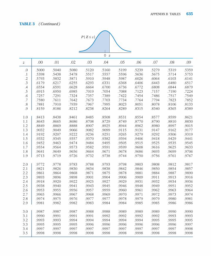
APPENDIX B TABLES 635
TABLE 3 (Continued)
z .00 .01 .02 .03 .04 .05 .06 .07 .08 .09
.0 .5000 .5040 .5080 .5120 .5160 .5199 .5239 .5279 .5319 .5359
.1 .5398 .5438 .5478 .5517 .5557 .5596 .5636 .5675 .5714 .5753
.2 .5793 .5832 .5871 .5910 .5948 .5987 .6026 .6064 .6103 .6141
.3 .6179 .6217 .6255 .6293 .6331 .6368 .6406 .6443 .6480 .6517
.4 .6554 .6591 .6628 .6664 .6700 .6736 .6772 .6808 .6844 .6879
.5 .6915 .6950 .6985 .7019 .7054 .7088 .7123 .7157 .7190 .7224
.6 .7257 .7291 .7324 .7357 .7389 .7422 .7454 .7486 .7517 .7549
.7 .7580 .7611 .7642 .7673 .7703 .7734 .7764 .7794 .7823 .7852
.8 .7881 .7910 .7939 .7967 .7995 .8023 .8051 .8078 .8106 .8133
.9 .8159 .8186 .8212 .8238 .8264 .8289 .8315 .8340 .8365 .8389
1.0 .8413 .8438 .8461 .8485 .8508 .8531 .8554 .8577 .8599 .86211.1 .8643 .8665 .8686 .8708 .8729 .8749 .8770 .8790 .8810 .88301.2 .8849 .8869 .8888 .8907 .8925 .8944 .8962 .8980 .8997 .90151.3 .9032 .9049 .9066 .9082 .9099 .9115 .9131 .9147 .9162 .91771.4 .9192 .9207 .9222 .9236 .9251 .9265 .9279 .9292 .9306 .93191.5 .9332 .9345 .9357 .9370 .9382 .9394 .9406 .9418 .9429 .94411.6 .9452 .9463 .9474 .9484 .9495 .9505 .9515 .9525 .9535 .95451.7 .9554 .9564 .9573 .9582 .9591 .9599 .9608 .9616 .9625 .96331.8 .9641 .9649 .9656 .9664 .9671 .9678 .9686 .9693 .9699 .97061.9 .9713 .9719 .9726 .9732 .9738 .9744 .9750 .9756 .9761 .9767
2.0 .9772 .9778 .9783 .9788 .9793 .9798 .9803 .9808 .9812 .98172.1 .9821 .9826 .9830 .9834 .9838 .9842 .9846 .9850 .9854 .98572.2 .9861 .9864 .9868 .9871 .9875 .9878 .9881 .9884 .9887 .98902.3 .9893 .9896 .9898 .9901 .9904 .9906 .9909 .9911 .9913 .99162.4 .9918 .9920 .9922 .9925 .9927 .9929 .9931 .9932 .9934 .99362.5 .9938 .9940 .9941 .9943 .9945 .9946 .9948 .9949 .9951 .99522.6 .9953 .9955 .9956 .9957 .9959 .9960 .9961 .9962 .9963 .99642.7 .9965 .9966 .9967 .9968 .9969 .9970 .9971 .9972 .9973 .99742.8 .9974 .9975 .9976 .9977 .9977 .9978 .9979 .9979 .9980 .99812.9 .9981 .9982 .9982 .9983 .9984 .9984 .9985 .9985 .9986 .9986
3.0 .9987 .9987 .9987 .9988 .9988 .9989 .9989 .9989 .9990 .99903.1 .9990 .9991 .9991 .9991 .9992 .9992 .9992 .9992 .9993 .99933.2 .9993 .9993 .9994 .9994 .9994 .9994 .9994 .9995 .9995 .99953.3 .9995 .9995 .9995 .9996 .9996 .9996 .9996 .9996 .9996 .99973.4 .9997 .9997 .9997 .9997 .9997 .9997 .9997 .9997 .9997 .99983.5 .9998 .9998 .9998 .9998 .9998 .9998 .9998 .9998 .9998 .9998
0 z
P [ Z ≤ z ]
bapp05.qxd 10/15/09 11:56 AM Page 635

636 APPENDIX B/TABLES
TABLE 4 Percentage Points of t Distributions
a
d.f. .25 .10 .05 .025 .01 .00833 .00625 .005
1 1.000 3.078 6.314 12.706 31.821 38.204 50.923 63.6572 .816 1.886 2.920 4.303 6.965 7.649 8.860 9.9253 .765 1.638 2.353 3.182 4.541 4.857 5.392 5.8414 .741 1.533 2.132 2.776 3.747 3.961 4.315 4.604
5 .727 1.476 2.015 2.571 3.365 3.534 3.810 4.0326 .718 1.440 1.943 2.447 3.143 3.287 3.521 3.7077 .711 1.415 1.895 2.365 2.998 3.128 3.335 3.4998 .706 1.397 1.860 2.306 2.896 3.016 3.206 3.3559 .703 1.383 1.833 2.262 2.821 2.933 3.111 3.250
10 .700 1.372 1.812 2.228 2.764 2.870 3.038 3.16911 .697 1.363 1.796 2.201 2.718 2.820 2.981 3.10612 .695 1.356 1.782 2.179 2.681 2.779 2.934 3.05513 .694 1.350 1.771 2.160 2.650 2.746 2.896 3.01214 .692 1.345 1.761 2.145 2.624 2.718 2.864 2.977
15 .691 1.341 1.753 2.131 2.602 2.694 2.837 2.94716 .690 1.337 1.746 2.120 2.583 2.673 2.813 2.92117 .689 1.333 1.740 2.110 2.567 2.655 2.793 2.89818 .688 1.330 1.734 2.101 2.552 2.639 2.775 2.87819 .688 1.328 1.729 2.093 2.539 2.625 2.759 2.861
20 .687 1.325 1.725 2.086 2.528 2.613 2.744 2.84521 .686 1.323 1.721 2.080 2.518 2.601 2.732 2.83122 .686 1.321 1.717 2.074 2.508 2.591 2.720 2.81923 .685 1.319 1.714 2.069 2.500 2.582 2.710 2.80724 .685 1.318 1.711 2.064 2.492 2.574 2.700 2.797
25 .684 1.316 1.708 2.060 2.485 2.566 2.692 2.78726 .684 1.315 1.706 2.056 2.479 2.559 2.684 2.77927 .684 1.314 1.703 2.052 2.473 2.552 2.676 2.77128 .683 1.313 1.701 2.048 2.467 2.546 2.669 2.76329 .683 1.311 1.699 2.045 2.462 2.541 2.663 2.756
30 .683 1.310 1.697 2.042 2.457 2.536 2.657 2.75040 .681 1.303 1.684 2.021 2.423 2.499 2.616 2.70460 .679 1.296 1.671 2.000 2.390 2.463 2.575 2.660
120 .677 1.289 1.658 1.980 2.358 2.428 2.536 2.617� .674 1.282 1.645 1.960 2.326 2.394 2.498 2.576
0 tα
α
bapp05.qxd 10/15/09 11:56 AM Page 636

APPENDIX B TABLES 637
TABLE 5 Percentage Points of x Distributions
a
d.f. .99 .975 .95 .90 .50 .10 .05 .025 .01
1 .0002 .001 .004 .02 .45 2.71 3.84 5.02 6.632 .02 .05 .10 .21 1.39 4.61 5.99 7.38 9.213 .11 .22 .35 .58 2.37 6.25 7.81 9.35 11.344 .30 .48 .71 1.06 3.36 7.78 9.49 11.14 13.285 .55 .83 1.15 1.61 4.35 9.24 11.07 12.83 15.096 .87 1.24 1.64 2.20 5.35 10.64 12.59 14.45 16.817 1.24 1.69 2.17 2.83 6.35 12.02 14.07 16.01 18.488 1.65 2.18 2.73 3.49 7.34 13.36 15.51 17.53 20.099 2.09 2.70 3.33 4.17 8.34 14.68 16.92 19.02 21.67
10 2.56 3.24 3.94 4.87 9.34 15.99 18.31 20.48 23.2111 3.05 3.81 4.57 5.58 10.34 17.28 19.68 21.92 24.7212 3.57 4.40 5.23 6.30 11.34 18.55 21.03 23.34 26.2213 4.11 5.01 5.89 7.04 12.34 19.81 22.36 24.74 27.6914 4.66 5.62 6.57 7.79 13.34 21.06 23.68 26.12 29.1415 5.23 6.26 7.26 8.55 14.34 22.31 25.00 27.49 30.5816 5.81 6.90 7.96 9.31 15.34 23.54 26.30 28.85 32.0017 6.41 7.56 8.67 10.09 16.34 24.77 27.59 30.19 33.4118 7.01 8.23 9.39 10.86 17.34 25.99 28.87 31.53 34.8119 7.63 8.90 10.12 11.65 18.34 27.20 30.14 32.85 36.19
20 8.26 9.59 10.85 12.44 19.34 28.41 31.41 34.17 37.5721 8.90 10.28 11.59 13.24 20.34 29.62 32.67 35.48 38.9322 9.54 10.98 12.34 14.04 21.34 30.81 33.92 36.78 40.2923 10.20 11.69 13.09 14.85 22.34 32.01 35.17 38.08 41.6424 10.86 12.40 13.85 15.66 23.34 33.20 36.42 39.36 42.9825 11.52 13.11 14.61 16.47 24.34 34.38 37.65 40.65 44.3126 12.20 13.84 15.38 17.29 25.34 35.56 38.89 41.92 45.6427 12.88 14.57 16.15 18.11 26.34 36.74 40.11 43.19 46.9628 13.56 15.30 16.93 18.94 27.34 37.92 41.34 44.46 48.2829 14.26 16.04 17.71 19.77 28.34 39.09 42.56 45.72 49.59
30 14.95 16.78 18.49 20.60 29.34 40.26 43.77 46.98 50.8940 22.16 24.42 26.51 29.05 39.34 51.81 55.76 59.34 63.6950 29.71 32.35 34.76 37.69 49.33 63.17 67.50 71.42 76.1560 37.48 40.47 43.19 46.46 59.33 74.40 79.08 83.30 88.3870 45.44 48.75 51.74 55.33 69.33 85.53 90.53 95.02 100.4380 53.54 57.15 60.39 64.28 79.33 96.58 101.88 106.63 112.3390 61.75 65.64 69.13 73.29 89.33 107.57 113.15 118.14 124.12
100 70.06 74.22 77.93 82.36 99.33 118.50 124.34 129.56 135.81
2
α
χ2α
bapp05.qxd 10/15/09 11:56 AM Page 637

638
TAB
LE 6
Per
cent
age
Poi
nts
of F
(,
) D
istr
ibut
ions
12
34
56
78
910
1215
2025
3040
60
139
.86
49.5
053
.59
55.8
357
.24
58.2
058
.91
59.4
459
.86
60.1
960
.71
61.2
261
.74
62.0
562
.26
62.5
362
.79
28.
539.
009.
169.
249.
299.
339.
359.
379.
389.
399.
419.
429.
449.
459.
469.
479.
473
5.54
5.46
5.39
5.34
5.31
5.28
5.27
5.25
5.24
5.23
5.22
5.20
5.18
5.17
5.17
5.16
5.15
44.
544.
324.
194.
114.
054.
013.
983.
953.
943.
923.
903.
873.
843.
833.
823.
803.
795
4.06
3.78
3.62
3.52
3.45
3.40
3.37
3.34
3.32
3.30
3.27
3.24
3.21
3.19
3.17
3.16
3.14
63.
783.
463.
293.
183.
113.
053.
012.
982.
962.
942.
902.
872.
842.
812.
802.
782.
767
3.59
3.26
3.07
2.96
2.88
2.83
2.78
2.75
2.72
2.70
2.67
2.63
2.59
2.57
2.56
2.54
2.51
83.
463.
112.
922.
812.
732.
672.
622.
592.
562.
542.
502.
462.
422.
402.
382.
362.
349
3.36
3.01
2.81
2.69
2.61
2.55
2.51
2.47
2.44
2.42
2.38
2.34
2.30
2.27
2.25
2.23
2.21
103.
292.
922.
732.
612.
522.
462.
412.
382.
352.
322.
282.
242.
202.
172.
162.
132.
1111
3.23
2.86
2.66
2.54
2.45
2.39
2.34
2.30
2.27
2.25
2.21
2.17
2.12
2.10
2.08
2.05
2.03
123.
182.
812.
612.
482.
392.
332.
282.
242.
212.
192.
152.
102.
062.
032.
011.
991.
9613
3.14
2.76
2.56
2.43
2.35
2.28
2.23
2.20
2.16
2.14
2.10
2.05
2.01
1.98
1.96
1.93
1.90
143.
102.
732.
522.
392.
312.
242.
192.
152.
122.
102.
052.
011.
961.
931.
911.
891.
8615
3.07
2.70
2.49
2.36
2.27
2.21
2.16
2.12
2.09
2.06
2.02
1.97
1.92
1.89
1.87
1.85
1.82
163.
052.
672.
462.
332.
242.
182.
132.
092.
062.
031.
991.
941.
891.
861.
841.
811.
7817
3.03
2.64
2.44
2.31
2.22
2.15
2.10
2.06
2.03
2.00
1.96
1.91
1.86
1.83
1.81
1.78
1.75
183.
012.
622.
422.
292.
202.
132.
082.
042.
001.
981.
931.
891.
841.
801.
781.
751.
7219
2.99
2.61
2.40
2.27
2.18
2.11
2.06
2.02
1.98
1.96
1.91
1.86
1.81
1.78
1.76
1.73
1.70
202.
972.
592.
382.
252.
162.
092.
042.
001.
961.
941.
891.
841.
791.
761.
741.
711.
6821
2.96
2.57
2.36
2.23
2.14
2.08
2.02
1.98
1.95
1.92
1.87
1.83
1.78
1.74
1.72
1.69
1.66
222.
952.
562.
352.
222.
132.
062.
011.
971.
931.
901.
861.
811.
761.
731.
701.
671.
6423
2.94
2.55
2.34
2.21
2.11
2.05
1.99
1.95
1.92
1.89
1.84
1.80
1.74
1.71
1.69
1.66
1.62
242.
932.
542.
332.
192.
102.
041.
981.
941.
911.
881.
831.
781.
731.
701.
671.
641.
6125
2.92
2.53
2.32
2.18
2.09
2.02
1.97
1.93
1.89
1.87
1.82
1.77
1.72
1.68
1.66
1.63
1.59
262.
912.
522.
312.
172.
082.
011.
961.
921.
881.
861.
811.
761.
711.
671.
651.
611.
5827
2.90
2.51
2.30
2.17
2.07
2.00
1.95
1.91
1.87
1.85
1.80
1.75
1.70
1.66
1.64
1.60
1.57
282.
892.
502.
292.
162.
062.
001.
941.
901.
871.
841.
791.
741.
691.
651.
631.
591.
5629
2.89
2.50
2.28
2.15
2.06
1.99
1.93
1.89
1.86
1.83
1.78
1.73
1.68
1.64
1.62
1.58
1.55
302.
882.
492.
282.
142.
051.
981.
931.
881.
851.
821.
771.
721.
671.
631.
611.
571.
5440
2.84
2.44
2.23
2.09
2.00
1.93
1.87
1.83
1.79
1.76
1.71
1.66
1.61
1.57
1.54
1.51
1.47
602.
792.
392.
182.
041.
951.
871.
821.
771.
741.
711.
661.
601.
541.
501.
481.
441.
4012
02.
752.
352.
131.
991.
901.
821.
771.
721.
681.
651.
601.
551.
481.
451.
411.
371.
32�
2.71
2.30
2.08
1.94
1.85
1.77
1.72
1.67
1.63
1.60
1.55
1.49
1.42
1.38
1.34
1.30
1.24
v 2v 1
��
.10
v 2v 1
Fα(v
1,
v 2)
α
bapp05.qxd 10/15/09 11:56 AM Page 638

639
TAB
LE 6
(Con
tinue
d)
12
34
56
78
910
1215
2025
3040
60
116
1.5
199.
521
5.7
224.
623
0.2
234.
023
6.8
238.
924
0.5
241.
924
3.9
246.
024
8.0
249.
325
0.1
251.
125
2.2
218
.51
19.0
019
.16
19.2
519
.30
19.3
319
.35
19.3
719
.38
19.4
019
.41
19.4
319
.45
19.4
619
.46
19.4
719
.48
310
.13
9.55
9.28
9.12
9.01
8.94
8.89
8.85
8.81
8.79
8.74
8.70
8.66
8.63
8.62
8.59
8.57
47.
716.
946.
596.
396.
266.
166.
096.
046.
005.
965.
915.
865.
805.
775.
755.
725.
695
6.61
5.79
5.41
5.19
5.05
4.95
4.88
4.82
4.77
4.74
4.68
4.62
4.56
4.52
4.50
4.46
4.43
65.
995.
144.
764.
534.
394.
284.
214.
154.
104.
064.
003.
943.
873.
833.
813.
773.
747
5.59
4.74
4.35
4.12
3.97
3.87
3.79
3.73
3.68
3.64
3.57
3.51
3.44
3.40
3.38
3.34
3.30
85.
324.
464.
073.
843.
693.
583.
503.
443.
393.
353.
283.
223.
153.
113.
083.
043.
019
5.12
4.26
3.86
3.63
3.48
3.37
3.29
3.23
3.18
3.14
3.07
3.01
2.94
2.89
2.86
2.83
2.79
104.
964.
103.
713.
483.
333.
223.
143.
073.
022.
982.
912.
852.
772.
732.
702.
662.
6211
4.84
3.98
3.59
3.36
3.20
3.09
3.01
2.95
2.90
2.85
2.79
2.72
2.65
2.60
2.57
2.53
2.49
124.
753.
893.
493.
263.
113.
002.
912.
852.
802.
752.
692.
622.
542.
502.
472.
432.
3813
4.67
3.81
3.41
3.18
3.03
2.92
2.83
2.77
2.71
2.67
2.60
2.53
2.46
2.41
2.38
2.34
2.30
144.
603.
743.
343.
112.
962.
852.
762.
702.
652.
602.
532.
462.
392.
342.
312.
272.
2215
4.54
3.68
3.29
3.06
2.90
2.79
2.71
2.64
2.59
2.54
2.48
2.40
2.33
2.28
2.25
2.20
2.16
164.
493.
633.
243.
012.
852.
742.
662.
592.
542.
492.
422.
352.
282.
232.
192.
152.
1117
4.45
3.59
3.20
2.96
2.81
2.70
2.61
2.55
2.49
2.45
2.38
2.31
2.23
2.18
2.15
2.10
2.06
184.
413.
553.
162.
932.
772.
662.
582.
512.
462.
412.
342.
272.
192.
142.
112.
062.
0219
4.38
3.52
3.13
2.90
2.74
2.63
2.54
2.48
2.42
2.38
2.31
2.23
2.16
2.11
2.07
2.03
1.98
204.
353.
493.
102.
872.
712.
602.
512.
452.
392.
352.
282.
202.
122.
072.
041.
991.
9521
4.32
3.47
3.07
2.84
2.68
2.57
2.49
2.42
2.37
2.32
2.25
2.18
2.10
2.05
2.01
1.96
1.92
224.
303.
443.
052.
822.
662.
552.
462.
402.
342.
302.
232.
152.
072.
021.
981.
941.
8923
4.28
3.42
3.03
2.80
2.64
2.53
2.44
2.37
2.32
2.27
2.20
2.13
2.05
2.00
1.96
1.91
1.86
244.
263.
403.
012.
782.
622.
512.
422.
362.
302.
252.
182.
112.
031.
971.
941.
891.
8425
4.24
3.39
2.99
2.76
2.60
2.49
2.40
2.34
2.28
2.24
2.16
2.09
2.01
1.96
1.92
1.87
1.82
264.
233.
372.
982.
742.
592.
472.
392.
322.
272.
222.
152.
071.
991.
941.
901.
851.
8027
4.21
3.35
2.96
2.73
2.57
2.46
2.37
2.31
2.25
2.20
2.13
2.06
1.97
1.92
1.88
1.84
1.79
284.
203.
342.
952.
712.
562.
452.
362.
292.
242.
192.
122.
041.
961.
911.
871.
821.
7729
4.18
3.33
2.93
2.70
2.55
2.43
2.35
2.28
2.22
2.18
2.10
2.03
1.94
1.89
1.85
1.81
1.75
304.
173.
322.
922.
692.
532.
422.
332.
272.
212.
162.
092.
011.
931.
881.
841.
791.
7440
4.08
3.23
2.84
2.61
2.45
2.34
2.25
2.18
2.12
2.08
2.00
1.92
1.84
1.78
1.74
1.69
1.64
604.
003.
152.
762.
532.
372.
252.
172.
102.
041.
991.
921.
841.
751.
691.
651.
591.
5312
03.
923.
072.
682.
452.
292.
182.
092.
021.
961.
911.
831.
751.
661.
601.
551.
501.
43�
3.84
3.00
2.61
2.37
2.21
2.10
2.01
1.94
1.88
1.83
1.75
1.67
1.57
1.51
1.46
1.39
1.32
v 2v 1
��
.05
Fα(v
1,
v 2)
α
bapp05.qxd 10/15/09 11:56 AM Page 639

640 APPENDIX B/TABLES
TABLE 7 Selected Tail Probabilities for the Null Distributionof Wilcoxon’s Rank-Sum Statistic
Smaller Sample Size � 2
Larger Sample Size
P � P [Ws � x ] � P [ Ws � x* ]
3
x P x*
8 .200 49 .100 3
10 0 2
4
x P x*
10 .133 411 .067 312 0 2
5
x P x*
11 .190 512 .095 413 .048 314 0 2
6
x P x*
13 .143 514 .071 415 .036 316 0 2
7
x P x*
15 .111 516 .056 417 .028 318 0 2
8
x P x*
16 .133 617 .089 518 .044 419 .022 320 0 2
9
x P x*
18 .109 619 .073 520 .036 421 .018 322 0 2
10
x P x*
19 .136 720 .091 621 .061 522 .030 423 .015 3
Smaller Sample Size � 3
Larger Sample Size3
x P x*
13 .200 814 .100 715 .050 616 0 5
4
x P x*
16 .114 817 .057 718 .029 619 0 5
5
x P x*
18 .125 919 .071 820 .036 721 .018 622 0 5
6
x P x*
20 .131 1021 .083 922 .048 823 .024 724 .012 625 0 5
7
x P x*
22 .133 1123 .092 1024 .058 925 .033 826 .017 727 .008 628 0 5
8
x P x*
24 .139 1225 .097 1126 .067 1027 .042 928 .024 829 .012 730 .006 631 0 5
9
x P x*
27 .105 1228 .073 1129 .050 1030 .032 931 .018 832 .009 7
10
x P x*
29 .108 1330 .080 1231 .056 1132 .038 1033 .024 934 .014 835 .007 7
bapp05.qxd 10/15/09 11:56 AM Page 640

APPENDIX B TABLES 641
TABLE 7 (Continued)
Smaller Sample Size � 4
Larger Sample Size4
x P x*
22 .171 1423 .100 1324 .057 1225 .029 1126 .014 1027 0 9
5
x P x*
25 .143 1526 .095 1427 .056 1328 .032 1229 .016 1130 .008 1031 0 9
6
x P x*
28 .129 1629 .086 1530 .057 1431 .033 1332 .019 1233 .010 11
7
x P x*
31 .115 1732 .082 1633 .055 1534 .036 1435 .021 1336 .012 1237 .006 11
8
x P x*
34 .107 1835 .077 1736 .055 1637 .036 1538 .024 1439 .014 1340 .008 12
9
x P x*
36 .130 2037 .099 1938 .074 1839 .053 1740 .038 1641 .025 1542 .017 1443 .010 13
10
x P x*
39 .120 2140 .094 2041 .071 1942 .053 1843 .038 1744 .027 1645 .018 1546 .012 1447 .007 13
Smaller Sample Size � 5
Larger Sample Size5
x P x*
34 .111 2135 .075 2036 .048 1937 .028 1838 .016 1739 .008 16
6
x P x*
37 .123 2338 .089 2239 .063 2140 .041 2041 .026 1942 .015 1843 .009 17
7
x P x*
41 .101 2442 .074 2343 .053 2244 .037 2145 .024 2046 .015 1947 .009 18
8
x P x*
44 .111 2645 .085 2546 .064 2447 .047 2348 .033 2249 .023 2150 .015 2051 .009 19
bapp05.qxd 10/15/09 11:56 AM Page 641

642 APPENDIX B/TABLES
TABLE 7 (Continued)
Larger Sample Size9
x P x*
47 .120 2848 .095 2749 .073 2650 .056 2551 .041 2452 .030 2353 .021 2254 .014 2155 .009 20
10
x P x*
51 .103 2952 .082 2853 .065 2754 .050 2655 .038 2556 .028 2457 .020 2358 .014 2259 .010 21
Smaller Sample Size � 6
Larger Sample Size6
x P x*
47 .120 3148 .090 3049 .066 2950 .047 2851 .032 2752 .021 2653 .013 2554 .008 24
7
x P x*
51 .117 3352 .090 3253 .069 3154 .051 3055 .037 2956 .026 2857 .017 2758 .011 2659 .007 25
8
x P x*
55 .114 3556 .091 3457 .071 3358 .054 3259 .041 3160 .030 3061 .021 2962 .015 2863 .010 27
9
x P x*
59 .112 3760 .091 3661 .072 3562 .057 3463 .044 3364 .033 3265 .025 3166 .018 3067 .013 2968 .009 28
10
x P x*
63 .110 3964 .090 3865 .074 3766 .059 3667 .047 3568 .036 3469 .028 3370 .021 3271 .016 3172 .011 3073 .008 29
bapp05.qxd 10/15/09 11:56 AM Page 642

APPENDIX B TABLES 643
TABLE 7 (Continued)
Smaller Sample Size � 7
Larger Sample Size7
x P x*
63 .104 4264 .082 4165 .064 4066 .049 3967 .036 3868 .027 3769 .019 3670 .013 3571 .009 34
8
x P x*
67 .116 4568 .095 4469 .076 4370 .060 4271 .047 4172 .036 4073 .027 3974 .020 3875 .014 3776 .010 36
9
x P x*
72 .105 4773 .087 4674 .071 4575 .057 4476 .045 4377 .036 4278 .027 4179 .021 4080 .016 3981 .011 3882 .008 37
10
x P x*
76 .115 5077 .097 4978 .081 4879 .067 4780 .054 4681 .044 4582 .035 4483 .028 4384 .022 4285 .017 4186 .012 4087 .009 39
Smaller Sample Size � 8
Larger Sample Size8
x P x*
80 .117 5681 .097 5582 .080 5483 .065 5384 .052 5285 .041 5186 .032 5087 .025 4988 .019 4889 .014 4790 .010 46
9
x P x*
86 .100 5887 .084 5788 .069 5689 .057 5590 .046 5491 .037 5392 .030 5293 .023 5194 .018 5095 .014 4996 .010 48
10
x P x*
91 .102 6192 .086 6093 .073 5994 .061 5895 .051 5796 .042 5697 .034 5598 .027 5499 .022 53
100 .017 52101 .013 51102 .010 50
bapp05.qxd 10/15/09 11:56 AM Page 643

644 APPENDIX B/TABLES
TABLE 7 (Continued)
Smaller Sample Size � 9
Larger Sample Size9
x P x*
100 .111 71101 .095 70102 .081 69103 .068 68104 .057 67105 .047 66106 .039 65107 .031 64108 .025 63109 .020 62110 .016 61111 .012 60112 .009 59
10
x P x*
106 .106 74107 .091 73108 .078 72109 .067 71110 .056 70111 .047 69112 .039 68113 .033 67114 .027 66115 .022 65116 .017 64117 .014 63118 .011 62119 .009 61
10
x P x*
122 .109 88123 .095 87124 .083 86125 .072 85126 .062 84127 .053 83128 .045 82129 .038 81130 .032 80131 .026 79132 .022 78133 .018 77134 .014 76135 .012 75136 .009 74
Smaller Sample Size � 10
Larger Sample Size
Source: Adapted from C. Kraft and C. van Eeden, A Nonparametric Introduction to Statistics,Macmillan, New York, 1968.
bapp05.qxd 10/15/09 11:56 AM Page 644

APPENDIX B TABLES 645
TABLE 8 Selected Tail Probabilities for the Null Distributionof Wilcoxon’s Signed-Rank Statistic
P � P [ T� � x ] � P [ T� � x* ]
x P x*
5 .250 16 .125 07 0
n � 3
x P x*
8 .188 29 .125 1
10 .062 011 0
n � 4
x P x*
12 .156 313 .094 214 .062 115 .031 016 0
n � 5
x P x*
17 .109 418 .078 319 .047 220 .031 121 .016 022 0
n � 6
x P x*
22 .109 623 .078 524 .055 425 .039 326 .023 227 .016 128 .008 0
n � 7
x P x*
27 .125 928 .098 829 .074 730 .055 631 .039 532 .027 433 .020 334 .012 235 .008 1
n � 8
x P x*
34 .102 1135 .082 1036 .064 937 .049 838 .037 739 .027 640 .020 541 .014 442 .010 3
n � 9
x P x*
40 .116 1541 .097 1442 .080 1343 .065 1244 .053 1145 .042 1046 .032 947 .024 848 .019 749 .014 650 .010 5
n � 10
x P x*
48 .103 1849 .087 1750 .074 1651 .062 1552 .051 1453 .042 1354 .034 1255 .027 1156 .021 1057 .016 958 .012 859 .009 7
n � 11
x P x*
56 .102 2257 .088 2158 .076 2059 .065 1960 .055 1861 .046 1762 .039 1663 .032 1564 .026 1465 .021 1366 .017 1267 .013 1168 .010 10
n � 12
x P x*
64 .108 2765 .095 2666 .084 2567 .073 2468 .064 2369 .055 2270 .047 2171 .040 2072 .034 1973 .029 1874 .024 1775 .020 1676 .016 1577 .013 1478 .011 1379 .009 12
n � 13
x P x*
73 .108 3274 .097 3175 .086 3076 .077 2977 .068 2878 .059 2779 .052 2680 .045 2581 .039 2482 .034 2383 .029 2284 .025 2185 .021 2086 .018 1987 .015 1888 .012 1789 .010 16
n � 14
bapp05.qxd 10/15/09 11:56 AM Page 645

646 APPENDIX B/TABLES
TABLE 8 (Continued)
x P x*
83 .104 3784 .094 3685 .084 3586 .076 3487 .068 3388 .060 3289 .053 3190 .047 3091 .042 2992 .036 2893 .032 2794 .028 2695 .024 2596 .021 2497 .018 2398 .015 2299 .013 21
100 .011 20101 .009 19
n � 15
Source: Adapted from C. Kraft and C. van Eeden, A Nonparametric Introduction to Statistics,Macmillan, New York, 1968.
bapp05.qxd 10/15/09 11:56 AM Page 646

The Jump River Electric Company serves several counties in northern Wisconsin. Much of the area is forest and lakes. The data on power outages froma recent summer include date, time, duration of outage (hours), and cause.
TABLE D.1 Power Outages
Date Time Duration Cause
6/11 4:00 PM 5.50 Trees and limbs6/12 8:00 PM 1.50 Trees and limbs6/16 8:30 AM 2.00 Trees and limbs6/17 5:30 AM 2.00 Trees and limbs6/17 5:00 PM 8.00 Windstorm6/21 4:30 PM 2.00 Trees and limbs6/26 3:00 AM 3.00 Trees and limbs6/26 2:00 PM 1.75 Unknown6/26 12:00 AM 2.00 Lightning blew up transformer7/03 6:00 PM 1.50 Trees and limbs7/04 9:00 AM 2.50 Unknown7/04 5:00 PM 1.50 Trees and limbs7/05 5:00 AM 1.50 Trees and limbs7/08 7:00 AM 3.50 Lightning7/20 12:00 AM 1.50 Unknown7/21 9:00 AM 1.50 Animal7/28 12:00 PM 1.00 Animal
Data Bank
bapp06.qxd 10/15/09 11:56 AM Page 647

648 DATA BANK
Madison recruits for the fire department need to complete a timed test thatsimulates working conditions. It includes placing a ladder against a building,pulling out a section of fire hose, dragging a weighted object, and crawling in asimulated attic environment. The times, in seconds, for recruits to complete thetest for a Madison firefighter are shown in Table D.2.
TABLE D.1 (Continued)
Date Time Duration Cause
7/30 7:00 PM 1.00 Squirrel on transformer7/31 7:30 AM 0.50 Squirrel on cutout8/04 6:00 AM 2.50 Trees and limbs8/06 8:00 PM 2.00 Beaver8/09 5:30 AM 1.50 Fuse-flying squirrel8/11 12:00 AM 3.00 Beaver-cut trees8/13 1:00 AM 1.00 Unknown8/15 12:30 AM 1.50 Animal8/18 8:00 AM 1.50 Trees and limbs8/20 4:00 AM 2.00 Transformer fuse8/25 9:00 AM 1.00 Animal8/26 2:00 AM 10.00 Lightning8/27 3:00 AM 1.00 Trees and limbs
TABLE D.2 Time to Complete Firefighters Physical Test (seconds)
425 389 380 421 438 331 368 417 403 416 385 315427 417 386 386 378 300 321 286 269 225 268 317287 256 334 342 269 226 291 280 221 283 302 308296 266 238 286 317 276 254 278 247 336 296 259270 302 281 228 317 312 327 288 395 240 264 246294 254 222 285 254 264 277 266 228 347 322 232365 356 261 293 354 236 285 303 275 403 268 250279 400 370 399 438 287 363 350 278 278 234 266319 276 291 352 313 262 289 273 317 328 292 279289 312 334 294 297 304 240 303 255 305 252 286297 353 350 276 333 285 317 296 276 247 339 328267 305 291 269 386 264 299 261 284 302 342 304336 291 294 323 320 289 339 292 373 410 257 406374 268
Natural resource managers have attempted to use the Satellite LandsatMultispectral Scanner data for improved land-cover classification. The intensi-ties of reflected light recorded on the near-infrared band of a thermatic mapperare given in Table D.3. Table D.3a gives readings from areas known to consist offorest and Table D.3b readings from urban areas.
bapp06.qxd 10/15/09 11:56 AM Page 648

DATA BANK 649
Beginning accounting students need to learn to audit in a computerized en-vironment. A sample of beginning accounting students took a test that is sum-marized by two scores shown in Table D.4: the Computer Attitude Scale(CAS), based on 20 questions, and the Computer Anxiety Rating Scale(CARS), based on 19 questions. (Courtesy of Douglas Stein.) Males are codedas 1 and females as 0.
TABLE D.4 Computer Attitude and Anxiety Scores
Gender CAS CARS Gender CAS CARS
0 2.85 2.90 1 3.30 3.471 2.60 2.32 1 2.90 3.050 2.20 1.00 1 2.60 2.681 2.65 2.58 0 2.25 1.901 2.60 2.58 0 1.90 1.841 3.20 3.05 1 2.20 1.741 3.65 3.74 0 2.30 2.580 2.55 1.90 0 1.80 1.581 3.15 3.32 1 3.05 2.471 2.80 2.74 1 3.15 3.320 2.40 2.37 0 2.80 2.901 3.20 3.11 0 2.35 2.420 3.05 3.32 1 3.70 3.471 2.60 2.79 1 2.60 4.001 3.35 2.95 0 3.50 3.420 3.75 3.79 0 2.95 2.530 3.00 3.26 1 2.80 2.681 2.80 3.21
TABLE D.3a Near Infrared Light Reflected from Forest Areas
77 77 78 78 81 81 82 82 82 82 82 83 83 84 84 84 84 8586 86 86 86 86 87 87 87 87 87 87 87 89 89 89 89 89 89 8990 90 90 91 91 91 91 91 91 91 91 91 91 93 93 93 93 93 9394 94 94 94 94 94 94 94 94 94 94 94 95 95 95 95 95 96 9696 96 96 96 97 97 97 97 97 97 97 97 97 98 99 100 100 100 100
100 100 100 100 100 101 101 101 101 101 101 102 102 102 102 102102 103 103 104 104 104 105 107
TABLE D.3b Near Infrared Light Reflected from Urban Areas
71 72 73 74 75 77 78 79 79 79 79 80 80 80 81 81 81 82 82 82 8284 84 84 84 84 84 85 85 85 85 85 85 86 86 87 88 90 91 94
bapp06.qxd 10/15/09 11:56 AM Page 649

650 DATA BANK
Data were collected on students taking the course Conditioning 1, designedto introduce students to a variety of training techniques to improve cardio-respiratory fitness, muscular strength, and flexibility (Table D.5). (Courtesy ofK. Baldridge.)
c1 Gender (1 � male, 2 � female)
c2 Pretest percent body fat
c3 Posttest percent body fat
c4 Pretest time to run 1.5 miles (seconds)
c5 Posttest time to run 1.5 miles (seconds)
c6 Pretest time to row 2.5 kilometers (seconds)
c7 Posttest time to row 2.5 kilometers (seconds)
c8 Pretest number of situps completed in 1 minute
c9 Posttest number of situps completed in 1 minute
TABLE D.5 Physical Fitness Improvement
Pretest Posttest Pretest Posttest Pretest Posttest Pretest PosttestGender % Fat % Fat Run Run Row Row Situps Situps
1 15.1 12.4 575 480 621 559 60 671 17.1 18.5 766 672 698 595 42 452 25.5 15.0 900 750 840 725 32 362 19.5 17.0 715 610 855 753 28 382 21.7 20.6 705 585 846 738 46 541 17.7 18.5 820 670 630 648 18 412 22.7 17.2 880 745 860 788 22 332 26.6 22.4 840 725 785 745 29 392 36.4 32.5 1065 960 780 749 27 401 9.7 8.0 630 565 673 588 32 492 31.0 25.0 870 780 746 689 39 542 6.0 6.0 580 494 756 714 37 492 25.1 22.8 1080 806 852 838 43 381 15.1 13.4 720 596 674 576 48 622 23.0 21.1 780 718 846 783 30 382 9.7 9.7 945 700 890 823 38 441 7.0 6.1 706 657 652 521 52 631 16.6 15.1 650 567 740 615 38 472 21.7 19.5 686 662 762 732 29 472 23.7 21.7 758 718 830 719 35 422 24.7 21.7 870 705 754 734 24 371 11.6 8.9 480 460 640 587 55 602 19.5 16.0 715 655 703 731 36 441 4.8 4.2 545 530 625 571 40 452 31.1 21.6 840 790 745 728 30 36
bapp06.qxd 10/15/09 11:56 AM Page 650

DATA BANK 651
TABLE D.5 (Continued)
Pretest Posttest Pretest Posttest Pretest Posttest Pretest PosttestGender % Fat % Fat Run Run Row Row Situps Situps
1 23.2 19.9 617 622 637 620 35 321 12.5 12.2 635 600 805 736 37 522 29.3 21.7 790 715 821 704 41 422 19.5 16.0 750 702 1043 989 42 451 10.7 9.8 622 567 706 645 40 462 26.6 21.7 722 725 741 734 49 612 27.6 23.7 641 598 694 682 40 471 25.9 18.8 708 609 685 593 20 211 27.5 16.0 675 637 694 682 35 371 9.4 7.6 618 566 610 579 36 501 12.5 9.8 613 552 610 575 46 502 27.5 30.9 705 660 746 691 31 362 18.3 15.0 853 720 748 694 31 341 6.6 4.7 496 476 623 569 45 452 23.7 21.7 860 750 758 711 42 552 23.2 22.1 905 636 759 726 26 302 18.0 14.8 900 805 823 759 31 292 22.7 18.3 767 741 808 753 28 321 19.9 14.8 830 620 632 586 39 451 6.6 5.7 559 513 647 602 44 491 14.3 9.8 699 652 638 602 34 351 21.7 18.5 765 735 674 615 41 481 13.9 9.4 590 570 599 571 40 421 20.1 19.3 770 672 675 611 37 481 15.1 8.9 602 560 656 578 47 582 14.8 11.0 741 610 768 687 34 412 23.4 19.1 723 641 711 695 36 412 23.7 16.3 648 601 802 740 44 511 28.0 17.7 842 702 790 765 26 291 4.7 4.7 558 540 660 600 40 462 26.6 23.7 750 565 720 670 36 522 21.7 18.3 608 592 707 697 42 461 11.6 8.9 537 495 610 572 55 602 22.7 18.3 855 694 800 712 41 502 21.7 18.3 630 614 785 743 50 552 25.9 21.9 902 820 771 717 34 381 28.4 21.7 780 664 756 703 57 642 21.9 20.8 665 670 673 667 41 442 27.5 22.7 675 646 689 674 49 501 5.7 3.8 473 472 551 546 53 532 22.7 22.0 715 682 678 672 40 432 33.2 25.7 795 740 817 721 30 312 16.0 13.6 688 615 811 705 45 491 14.3 11.6 530 497 589 570 39 50
bapp06.qxd 10/15/09 11:56 AM Page 651

652 DATA BANK
TABLE D.5 (Continued)
Pretest Posttest Pretest Posttest Pretest Posttest Pretest PosttestGender % Fat % Fat Run Run Row Row Situps Situps
1 22.7 19.5 840 705 788 780 29 322 25.0 18.3 690 618 816 701 42 501 4.2 3.2 545 527 577 543 55 592 25.7 21.7 760 727 849 724 39 441 13.9 9.4 620 515 689 580 32 411 12.2 7.6 605 564 661 614 35 381 21.7 20.6 688 625 750 686 39 321 7.0 5.1 590 529 631 619 60 652 34.6 27.5 720 694 690 698 34 451 3.2 3.2 500 459 644 599 35 371 6.1 5.1 540 492 579 546 56 602 28.4 21.7 885 825 804 733 33 36
bapp06.qxd 10/15/09 11:56 AM Page 652

DATA BANK 653
Grizzly bears are magnificent animals that weigh up to several hundredpounds and can run over 30 mph in short distances. Males range over severalmiles but the females tend to stay closer to home. Grizzly bears usually keep tothemselves. However, several grizzly bear attacks on humans are reported eachyear. Because of their large size, they can menace hikers and campers in somecircumstances. Even so, it is important that a healthy grizzly bear population bemaintained for future generations.
Harry Reynolds, of the Alaska Game and Fish Department, has studied griz-zly bears for over 20 years in an effort to protect them and learn what they needto survive. He and his colleagues typically spot bears from an airplane. Oncea bear is located, they try to shoot it with a dart so that it falls asleep for a fewminutes. During this brief period, they check its overall health and take mea-surements of the size of the bear. They also roll the bear onto a tarp, which isthen lifted by a scale attached to a tripod. Age is given in years, weight inpounds, and the other size measurements in centimeters.
Occasionally, the researchers have to run to a vehicle for protection whenthe sedated bear awakes too quickly. These measurements are not easy to make!
TABLE D.6 Grizzly Bear Data
Head HeadBear Sex Age Weight Length Neck Girth Length Width
1 M 9 245 199 84 135 24.5 39.02 M 9 200 198 83 129 22.5 39.33 F 4 102 174 65 104 20.3 33.44 F 5 180 183 57 101 17.9 32.75 F 5 225 170 57 100 18.6 33.36 F 5 230 188 62 103 19.3 32.97 F 13 315 185 62 118 22.1 36.98 F 19 280 193 63 114 22.2 35.59 F 5 235 177 56 93 19.4 33.4
10 F 2 70 152 46 80 16.8 31.311 M 2 91 157 58 102 17.3 30.612 F 6 280 181 61 100 19.4 34.513 M 11 465 204 84 132 23.7 38.814 M 4 125 191 60 97 20.1 33.415 F 6 265 189 59 100 20.4 33.316 F 3 107 156 45 81 16.3 28.117 F 2 68 158 43 77 16.0 29.918 M 2 75 163 45 77 17.8 29.719 M 2 82 164 48 80 16.7 32.320 F 6 245 176 66 104 20.5 34.521 F 4 215 176 55 103 19.1 32.022 M 2 84 169 53 89 19.9 31.523 F 17 109 176 62 112 19.0 32.324 F 5 240 185 61 103 20.5 33.625 F 5 247 175 57 102 18.5 33.3
bapp06.qxd 10/15/09 11:56 AM Page 653

654 DATA BANK
TABLE D.6 (Continued)
Head HeadBear Sex Age Weight Length Neck Girth Length Width
26 F 3 130 148 45 77 13.6 27.427 F 3 130 166 53 86 17.5 30.028 F 7 280 177 57 106 18.7 33.129 M 11 620 224 95 164 24.2 42.030 M 3 150 151 49 85 18.0 32.431 F 1 115 134 45 78 14.4 26.532 F 1 115 137 43 77 14.0 26.833 F 4 285 188 64 110 19.6 34.034 M 4 415 199 77 137 23.0 38.535 F 1 120 135 49 77 14.0 26.336 M 6 578 219 90 134 24.8 38.637 M 2 140 148 56 88 17.0 29.938 F 2 125 131 48 80 16.3 27.239 M 4 265 178 63 102 18.8 32.240 F 2 135 153 49 83 16.2 28.741 M 2 212 171 51 88 17.8 31.442 F 2 190 168 49 81 17.4 30.343 M 5 359 198 76 114 21.4 36.644 F 7 187 166 57 95 19.4 32.445 M 1 62 114 37 66 12.4 26.946 F 17 283 188 67 113 20.5 37.047 M 1 126 145 46 84 15.2 27.448 F 4 196 168 56 90 18.2 31.549 M 4 345 192 69 112 20.3 35.250 M 2 195 175 53 92 18.2 30.251 M 1 100 125 41 73 14.1 24.552 F 1 50 107 33 58 12.1 21.153 M 1 100 131 45 74 15.1 26.754 F 1 65 119 39 53 13.2 22.555 F 1 105 136 42 71 15.0 25.556 M 1 110 144 43 70 15.4 26.557 F 1 100 133 45 66 16.4 25.258 M 1 63 116 38 62 13.3 23.559 F 1 70 123 41 63 13.5 24.260 F 1 96 139 46 76 14.5 25.661 M 1 95 142 48 76 14.4 25.6
bapp06.qxd 10/15/09 11:56 AM Page 654

DATA BANK 655
Salmon fisheries support a primary industry in Alaska and their management isof high priority. Salmon are born in freshwater rivers and streams, but then swimout into the ocean for a few years before returning to spawn and die. In order toidentify the origins of mature fish and equably divide the catch of returning salmonbetween Alaska and the Canadian provinces, researchers have studied the growthof their scales. The growth the first year in freshwater is measured by the width ofthe growth rings for that period of life, and marine growth is measured by thewidth of the growth rings for the first year in the ocean environment. The scalesare first magnified 100 times and then the measurements are made in hundredthsof an inch. A set of these measurements, collected by the Alaska Department ofFish and Game, are given in Table D.7. (Courtesy of K. Jensen and B. Van Alen.)
TABLE D.7 Radius of Growth Zones for Freshwater and First Marine Year
Males Females
Freshwater First Year Freshwater First YearGrowth Marine Growth Growth Marine Growth
147 444 131 405139 446 113 422160 438 137 42899 437 121 469
120 405 139 424151 435 144 402115 394 161 440121 406 107 410109 440 129 366119 414 123 422130 444 148 410110 465 129 352127 457 119 414100 498 134 396115 452 139 473117 418 140 398112 502 126 434116 478 116 39598 500 112 33498 589 117 45583 480 97 43985 424 134 51188 455 88 43298 439 99 38174 423 105 41858 411 112 475
114 484 98 43688 447 80 431
bapp06.qxd 10/15/09 11:56 AM Page 655

656 DATA BANK
TABLE D.7 (Continued)
Males Females
Freshwater First Year Freshwater First YearGrowth Marine Growth Growth Marine Growth
77 448 139 51586 450 97 50886 493 103 42965 495 93 420
127 470 85 42491 454 60 45676 430 115 49144 448 113 47442 512 91 42150 417 109 45157 466 122 44242 496 68 363
The U. S. Department of Agriculture and State Agriculture Experiment Sta-tions cooperate on the investigation of barleys for possible use in brewingprocesses. One year, the malt extract (%) was obtained for 40 different varietiesfrom one experiment station.
TABLE D.8 Malt Extract
75.3 77.9 77.6 76.6 78.3 77.9 77.5 77.6 77.1 78.077.9 76.3 75.7 77.4 77.4 76.9 77.9 77.4 78.1 77.476.4 79.1 80.0 76.9 78.5 78.4 77.8 80.4 75.9 77.079.2 76.2 77.0 75.9 77.9 78.4 76.7 76.4 76.6 77.4
bapp06.qxd 10/15/09 11:56 AM Page 656

DATA BANK 657
An ongoing study of wolves is being conducted at the Yukon-Charley RiversNational Preserve. Here are some of the physical characteristics of wolves thatwere observed. (Courtesy of John Burch National Park Service, Fairbanks, Alaska.)
TABLE D.9 Physical Characteristics of Wolves
Body Tail CanineSex Age Weight ( lb) Length (cm) Length (cm) Length (mm)
M 4 71 134 44 28.7F 2 57 123 46 27.0F 4 84 129 49 27.2M 4 93 143 46 30.5M 4 101 148 48 32.3M 1 84 127 42 25.8M 2 88 136 47 26.6M 3 117 146 46 29.1F 2 90 143 43 27.1M 4 86 142 51 29.2F 6 71 124 42 28.2F 8 71 125 42 27.8M 0 86 139 54 24.0M 2 93 140 45 29.0M 2 86 133 44 29.3F 3 77 122 45 27.4F 2 68 125 51 27.3M 3 106 123 53 29.0F 0 73 122 43 24.5
bapp06.qxd 10/15/09 11:56 AM Page 657

658 DATA BANK
Researchers studying sleep disorders needed to obtain data from the generalpopulation to serve as a reference set. They randomly selected state employeeswho worked in certain divisions, and many agreed to spend a night in the sleeplab and be measured. Female � 0 and male � 1. The body weight index(BMI) is a person’s weight (kg) divided by the square of his or her height (m).The percent of rapid eye movement (PREM) sleep is the percent of total sleeptime that is spent in rapid eye movement sleep. The number of breathing pausesper hour (BPH) is the total number of breathing pauses divided by the totalhours of sleep. The snoring frequency (SNORF) is a response to the surveyquestion, “According to what others have told you, please estimate how oftenyou snore?” The possible responses were (1) rarely, (2) sometimes, (3) irregularpattern but at least once a week, (4) three to five nights a week, or (5) every oralmost every night. (Courtesy of T. Young.)
TABLE D.10 Sleep Data
Gender Age BMI PREM BPH SNORF Gender Age BMI PREM BPH SNORF
0 41 24.65 0.200 0.00 5 0 55 25.10 0.326 0.19 00 49 23.14 0.162 0.00 4 0 31 28.17 0.124 0.21 10 39 27.61 0.308 0.00 5 0 58 32.68 0.216 5.76 10 51 33.50 0.083 0.00 4 0 43 20.07 0.191 0.00 00 32 43.36 0.205 2.79 4 0 53 24.92 0.189 7.46 00 37 31.04 0.109 3.87 5 0 52 29.10 0.194 0.69 20 36 32.42 0.154 0.00 5 0 43 26.40 0.077 0.00 20 30 31.06 0.328 3.42 5 0 41 20.13 0.138 0.12 10 44 44.15 0.227 4.39 5 0 34 23.77 0.260 0.00 00 43 38.29 0.104 5.14 5 0 41 29.06 0.163 0.31 20 34 21.63 0.184 0.00 5 0 49 24.45 0.164 0.00 00 47 34.78 0.215 1.13 5 0 41 21.15 0.142 0.41 00 40 25.16 0.206 0.00 2 0 47 19.47 0.224 0.00 10 49 37.02 0.123 2.58 5 0 59 28.76 0.176 0.99 00 54 31.25 0.313 0.00 0 0 34 26.77 0.109 0.00 00 38 32.58 0.227 0.13 5 0 42 40.06 0.191 0.14 00 36 34.65 0.172 0.00 4 0 44 24.99 0.316 1.01 20 39 29.55 0.223 2.84 5 0 32 17.86 0.174 0.00 00 45 31.96 0.146 0.00 4 0 31 25.99 0.109 0.00 00 49 21.64 0.250 0.00 5 0 35 20.42 0.227 0.25 20 47 30.67 0.244 3.98 5 0 58 23.03 0.202 0.00 10 33 23.43 0.228 0.00 2 0 38 41.14 0.220 1.24 20 43 30.24 0.193 0.00 1 0 40 22.49 0.149 0.00 00 43 37.83 0.230 7.11 5 0 43 23.71 0.149 0.00 00 39 22.46 0.141 0.17 5 1 44 30.22 0.162 2.33 50 50 33.53 0.094 3.66 5 1 59 27.39 0.103 0.00 30 57 24.35 0.174 0.33 4 1 51 24.34 0.203 1.30 50 36 37.64 0.000 25.36 2 1 49 27.17 0.179 0.00 50 34 28.03 0.205 0.00 1 1 29 28.09 0.228 0.00 40 43 25.24 0.223 0.00 1 1 40 30.06 0.180 3.18 50 59 33.71 0.175 4.71 0 1 45 40.82 0.082 2.34 5
bapp06.qxd 10/15/09 11:56 AM Page 658

DATA BANK 659
TABLE D.10 (Continued)
Gender Age BMI PREM BPH SNORF Gender Age BMI PREM BPH SNORF
1 55 32.46 0.082 38.00 5 1 47 24.00 0.220 0.53 51 51 22.95 0.175 3.29 4 1 36 31.76 0.196 6.73 51 38 21.97 0.123 0.00 5 1 59 27.12 0.255 6.18 51 36 25.57 0.179 0.00 4 1 42 24.34 0.137 1.46 51 39 26.67 0.216 0.24 5 1 59 35.14 0.160 3.56 51 38 28.95 0.231 0.55 5 1 37 26.53 0.122 3.80 41 42 35.65 0.139 0.20 5 1 55 31.28 0.170 0.58 41 34 43.65 0.131 47.52 4 1 31 35.61 0.066 19.60 41 55 42.70 0.191 5.41 5 1 53 27.55 0.083 8.01 41 42 25.04 0.242 0.00 5 1 41 34.92 0.207 15.28 41 47 31.28 0.147 7.26 5 1 45 33.20 0.228 4.37 51 46 31.02 0.124 22.55 5 1 41 29.94 0.134 2.42 51 39 25.43 0.169 10.35 5 1 50 26.26 0.179 0.16 51 37 26.29 0.178 7.05 5 1 40 34.94 0.174 8.76 51 41 29.59 0.259 1.37 5 1 54 28.60 0.197 0.00 41 58 29.24 0.170 3.89 5 1 39 31.55 0.135 0.81 51 57 28.72 0.152 2.33 5 1 49 22.84 0.109 1.53 21 33 28.56 0.126 1.09 5 1 46 18.89 0.114 0.00 01 58 30.04 0.160 0.18 4 1 39 25.70 0.233 0.00 01 54 35.43 0.117 1.24 5 1 41 26.89 0.247 1.94 11 46 34.78 0.151 19.47 5 1 46 31.29 0.230 0.00 21 46 25.66 0.223 0.00 3 1 40 29.76 0.000 0.71 01 55 31.80 0.087 4.58 5 1 44 26.71 0.163 0.39 21 56 29.74 0.162 18.77 5 1 41 24.69 0.209 0.16 01 35 24.43 0.423 0.16 5 1 37 26.58 0.074 0.00 01 49 23.33 0.196 21.58 4 1 44 23.61 0.234 0.00 01 50 26.45 0.199 0.00 4 1 44 29.86 0.147 5.13 21 42 27.38 0.155 2.63 5 1 41 28.41 0.097 0.19 11 46 27.06 0.123 0.00 5 1 46 23.12 0.156 0.19 01 37 24.82 0.175 0.18 4 1 34 29.88 0.195 0.00 01 38 30.64 0.190 70.82 5 1 41 18.02 0.149 0.00 01 44 37.61 0.254 7.61 5 1 44 20.90 0.181 0.21 01 48 26.85 0.219 0.42 4 1 39 22.39 0.223 0.00 11 53 28.23 0.103 0.33 4 1 35 29.23 0.152 0.00 21 55 29.48 0.150 4.57 5 1 38 23.83 0.163 0.00 21 56 27.76 0.185 7.82 5 1 47 22.23 0.129 0.76 11 57 32.08 0.205 28.26 5 1 47 28.04 0.146 2.53 01 58 27.55 0.128 26.37 5 1 50 32.82 0.183 12.86 01 37 31.98 0.241 5.38 1 1 48 20.09 0.083 1.59 21 30 24.09 0.188 0.68 5 1 38 26.63 0.229 1.81 21 51 33.80 0.169 0.90 5 1 37 30.72 0.203 2.13 21 44 28.08 0.130 0.53 5 1 50 24.73 0.188 0.00 21 45 30.83 0.105 6.86 4 1 37 33.35 0.274 17.78 2
1 44 24.70 0.170 0.42 21 49 18.24 0.223 0.00 11 41 24.86 0.216 2.31 0
bapp06.qxd 10/15/09 11:56 AM Page 659

660 DATA BANK
Insecticides, including the long banned DDT, which imitate the human re-productive hormone estrogen, may cause serious health problems in humansand animals. Researchers examined the reproductive development of young alli-gators hatched from eggs taken from (1) Lake Apopka, which is adjacent to anEPA Superfund site, and (2) Lake Woodruff, which acted as a control. The con-taminants at the first lake, including DDT, were thought to have caused repro-ductive disorders in animals living in and around the lake. The concentrations ofthe sex steroids estradiol and testosterone in the blood of alligators were deter-mined by radioimmunoassay both at about six months of age and then again af-ter the alligators were stimulated with LH, a pituitary hormone. (Courtesy of L.Guillette.)
The data are coded as (* indicates missing):
� 1, Lake Apopka, and � 0, Lake Woodruff
� 1 male and � 0 female
� E2 � estradiol concentration (pg/ml)
� T � testosterone concentration (pg/ml)
� LHE2 � estradiol concentration after receiving LH (pg/ml)
� LHT � testosterone concentration after receiving LH (pg/ml)x6
x5
x4
x3
x2
x1
TABLE D.11 Alligator Data
Lake Apopka Lake Woodruff
Lake Sex E2 T LHE2 LHT Lake Sex E2 T LHE2 LHT
1 1 38 22 134 15 0 1 29 47 46 101 1 23 24 109 28 0 1 64 20 82 761 1 53 8 16 12 0 1 19 60 * *1 1 37 6 220 13 0 1 36 75 19 721 1 30 7 114 11 0 1 27 12 118 951 0 60 19 184 7 0 1 16 54 33 641 0 73 23 143 13 0 1 15 33 99 191 0 64 16 228 13 0 1 72 53 29 201 0 101 8 163 10 0 1 85 100 72 01 0 137 9 83 7 0 0 139 20 82 21 0 88 7 200 12 0 0 74 4 170 751 0 73 19 220 21 0 0 83 18 125 451 0 257 8 194 37 0 0 35 43 19 761 0 138 10 221 3 0 0 106 9 142 51 0 220 15 101 5 0 0 47 52 24 621 0 88 10 141 7 0 0 38 8 68 20
0 0 65 15 32 500 0 21 7 140 40 0 68 16 110 30 0 70 16 58 180 0 112 14 78 5
x6x5x4x3x2x1x6x5x4x3x2x1
bapp06.qxd 10/15/09 11:56 AM Page 660

TABLE D.12 Credit Card Data
Row Gender Age Charge FreqCC Charity Compassion
1 0 3 100 1 6 62 1 3 150 3 5 73 0 3 500 3 7 74 1 3 0 1 5 75 1 3 0 2 6 66 0 1 100 4 5 57 1 3 1100 6 6 68 1 3 1000 5 5 79 0 3 200 6 7 710 1 3 1000 5 7 711 1 2 200 5 7 712 1 1 500 4 5 513 1 3 100 4 5 614 1 3 20 3 6 715 0 3 0 1 7 716 0 2 400 6 6 517 1 1 0 1 5 718 1 3 0 1 6 619 0 1 800 7 6 520 1 3 1000 7 7 721 1 1 100 4 5 422 1 3 500 4 5 523 1 3 0 4 4 524 1 2 300 4 5 525 1 2 400 5 5 526 1 1 50 4 6 7
DATA BANK 661
Market researchers track attitudes and preferences of potential purchasers.An increasing number of brands are being linked to social causes and this studywas conducted to help determine if adding a social cause to products wouldcause a difference in consumers’ preferences regarding credit cards. Questionsabout credit card use and preferences, as well as attitudes toward sharing wealthwith others, were included.
Female � 0 and male � 1. The three age groups 19–24, 25–34, and35–44 are coded as 1, 2, and 3, respectively. Charge is the average monthlyamount charged on credit cards. The last three variables are measured on sevenpoint rating scales. The frequency of credit card use, FreqCC, ranges from never(1) to several times a day (7), with weekly (4) in the middle. “Money given tocharities goes for good causes” and “I consider myself a compassionate person”scored from strongly disagree (1) to strongly agree (7). (Courtesy of NeerajArora)
2
N. Arora and T. Henderson. “Embedded Premium Promotion: Why it Works and How to Make itMore Effective,” Marketing Science, 26, (2007), pp. 514–531.
2
bapp06.qxd 10/15/09 11:56 AM Page 661

TABLE D.12 (Continued)
Row Gender Age Charge FreqCC Charity Compassion
27 1 2 100 4 6 628 1 2 200 5 4 729 0 2 1 6 5 530 1 2 2000 7 1 431 1 1 450 3 7 732 1 2 100 2 3 633 1 3 0 1 5 634 1 2 600 4 6 635 1 3 100 3 6 736 1 3 700 5 7 737 1 3 500 4 6 738 1 2 300 7 6 639 1 3 100 4 7 740 1 3 1500 7 7 541 0 3 600 6 6 642 1 1 40 2 6 743 1 2 1000 7 4 544 1 3 100 3 6 745 1 2 300 3 6 646 1 1 0 1 7 747 1 3 150 5 6 648 1 2 10 2 6 749 0 2 1000 5 7 750 1 2 500 5 7 751 0 3 0 2 4 652 0 1 500 4 5 453 1 2 450 4 5 554 1 2 200 5 6 755 1 2 25 3 2 656 1 2 500 5 5 657 1 3 70 4 2 458 0 3 300 4 5 159 1 3 300 5 4 660 1 1 0 2 4 661 1 1 0 1 5 662 1 2 200 5 5 563 0 2 2000 4 4 464 0 3 0 1 7 765 1 3 1500 7 4 566 1 2 0 1 3 367 1 1 60 3 6 668 1 3 500 5 7 769 0 3 0 1 5 770 0 3 1200 5 5 671 0 3 2000 6 5 5
662 DATA BANK
bapp06.qxd 10/15/09 11:56 AM Page 662
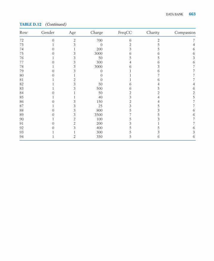
TABLE D.12 (Continued)
Row Gender Age Charge FreqCC Charity Compassion
72 0 2 700 6 2 773 1 3 0 2 5 474 0 1 200 3 5 675 0 3 3000 6 6 676 1 3 50 5 5 377 0 3 300 4 6 678 1 3 3000 6 3 779 0 3 0 1 6 780 0 1 0 1 7 781 1 2 0 1 6 782 1 3 50 6 4 483 1 3 500 6 5 684 0 1 50 2 2 285 1 1 40 3 4 586 0 3 150 2 4 787 1 3 25 3 5 788 0 3 800 5 3 689 0 3 3500 7 5 690 1 2 100 5 3 791 0 2 200 3 1 792 0 3 400 5 5 693 1 1 300 5 3 394 1 2 350 5 6 6
DATA BANK 663
bapp06.qxd 10/15/09 11:56 AM Page 663

bapp06.qxd 10/15/09 11:56 AM Page 664

CHAPTER 1
1.1 Population: Entire set of responses from all U.S. teens 13 to 17. Sample: re-sponses from the 1055 teens contacted.
1.3 (a) person living in Chicago, (b) whethera person is an illegal alien(yes) or not (no),(c) entire set of yes/no responses from allpersons living in Chicago.
1.5 (a) Anyone who golfs (b) The statisticalpopulation is the collection of estimatedhole sizes, one for each golfer. The sam-ple is the collection of 46 hole sizes thepsychologists recorded.
1.7 It is likely that any person visiting the sitedoes so because they have a problem withprocrastination.The scores recordedwould not be representative of the generalpopulation.
Answers to Selected Odd-Numbered Exercises
1.9 Population: The entire collection ofresponses, from all residents, of theirfavorite establishment. Sample: theresponses from the persons who filledout the form. This is a self-selectedsample, and not representative, as onlythose with strong opinions would fill out form.
1.11 (a) anecdotal, ( b) sample based,(c) sample based
1.13 “Too long” is not well defined. Could, forinstance, say half the time it takes longerthan 5 minutes.
1.21 (b) Including votes only from those withstrong enough opinions to call in, like bigdogs jumping above the fence, would pro-duce unrepresentative results.
bansw.qxd 10/15/09 11:50 AM Page 665
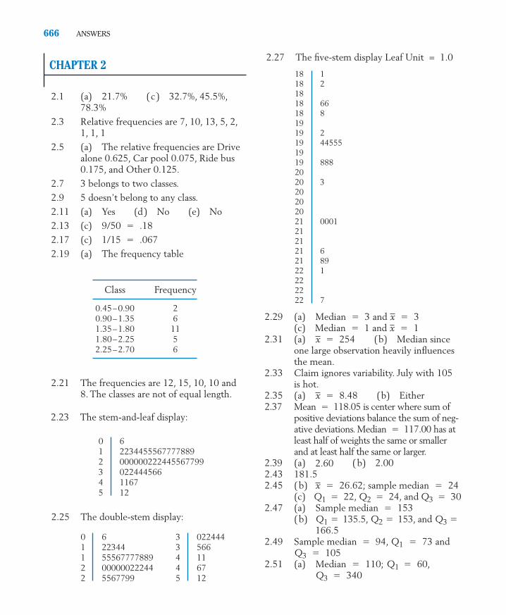
666 ANSWERS
2.29 (a) Median � 3 and (c) Median � 1 and
2.31 (a) (b) Median sinceone large observation heavily influencesthe mean.
2.33 Claim ignores variability. July with 105is hot.
2.35 (a) (b) Either2.37 Mean � 118.05 is center where sum of
positive deviations balance the sum of neg-ative deviations. Median � 117.00 has atleast half of weights the same or smallerand at least half the same or larger.
2.39 (a) 2.60 (b) 2.002.43 181.52.45 (b)
(c)2.47 (a)
(b) � 135.5, � 153, and �166.5
2.49 Sample median � 94, � 73 and� 105
2.51 (a)Q3 � 340
Q1 � 60,Median � 110;Q3
Q1
Q3Q2Q1
Sample median � 153Q1 � 22, Q2 � 24, and Q3 � 30x � 26.62; sample median � 24
x � 8.48
x � 254x � 1x � 3
CHAPTER 2
2.1 (a) 21.7% (c) 32.7%, 45.5%,78.3%
2.3 Relative frequencies are 7, 10, 13, 5, 2,1, 1, 1
2.5 (a) The relative frequencies are Drivealone 0.625, Car pool 0.075, Ride bus0.175, and Other 0.125.
2.7 3 belongs to two classes.
2.9 5 doesn’t belong to any class.
2.11 (a) Yes (d) No (e) No
2.13 (c) 9/50 � .18
2.17 (c) 1/15 � .067
2.19 (a) The frequency table
2.23 The stem-and-leaf display:
Class Frequency
0.45–0.90 20.90–1.35 61.35–1.80 111.80–2.25 52.25–2.70 6
2.25 The double-stem display:
0 61 22344555677778892 0000002224455677993 0224445664 11675 12
2.27 The five-stem display Leaf Unit = 1.0
0 61 223441 555677778892 000000222442 5567799
3 0224443 5664 114 675 12
18 118 21818 6618 81919 219 445551919 8882020 320202021 0001212121 621 8922 1222222 7
2.21 The frequencies are 12, 15, 10, 10 and8. The classes are not of equal length.
bansw.qxd 10/15/09 11:50 AM Page 666

ANSWERS 667
(b)2.53 (b) Mean � 24.33°C; median �
24.44°C2.57 (b)2.59 (b)2.63 (a) (c)2.67 (a) (b) s � 393.992.71 (a) Median � 68.4
(b) (c) s � 2.4192.73 (a) (b) 25.00
(c) 8 is nearly half as variable.2.75 Interquartile range � 31.02.77 No. Extremes more variable than middle.2.81 (a) and s � 1.303 (b)
proportions .5, 1.0 and 1.0, respectively.2.83 (a) �1.037 (b) 1.6772.87 (a) Mean � 24.83, standard devia-
tion � 7.68 (b) 23/24 � .9582.89 Mean � 1.925, standard devia-
tion � 1.6072.91 (a) 14.0 (b) maximum 55 Truman
and minimum � 8 (gain) Bush (c) 632.95 Only the value 215 from the second
period is outside of limits.2.97 First an upward trend and then a down-
ward trend. Control limits not appropriate.2.99 The relative frequencies of the occupa-
tion groups are:
x � 2.600
s2 � 239.32x � 68.343
s2 � 155,226s2 � .286s2 � 1.30
s2 � 18.667 and s � 4.32s2 � 7 and s � 2.646
90th percentile � 400 2.109 (a) (c) Mean� � 21, standard deviation � 6.
2.113 (a) (b)Median � 5.0 (c) Range � 13
2.115 (a) Median � 4.505,(b) 4.935
(c)2.117 (a) Median � 6.7,
7.1(b) and s � .466
2.119 (b) Not reasonable with time trend2.121 Mean � 83.34 and standard deviation
� 38.372.129
CHAPTER 3
3.1 (c) The pill seems to reduce the propor-tions of severe and moderate nausea.
3.3 The proportion who study more than 10hours is highest for the physical sciences.It is .70 while social sciences have thelowest proportion .48.
3.7 (b)
x � 109.1, s � 65.8
x � 6.73
Q1 � 6.4, Q3 �x � 4.5074, s � .368Q3 � 4.70
Q1 � 4.30,
x � 5.375 and s � 3.424
x � 7, s � 2
2.103 (a) Yes (b) Yes (c ) No2.105 (a) Mean = 227.4 pounds is center
where sum of positive deviations balancethe sum of negative deviations. Median �232.5 has at least half of weights the sameor smaller and at least half the same orlarger. (b) 82.7 (c) 1.120
2.107 (a) Median � 9 (b)(c) � 3.895s2
x � 9.033
Occupation Relative FrequencyGroup 2007 2000
Goods producing 0.139 0.161Service (private) 0.722 0.702Government 0.139 0.136
Total 1.000 0.999
MajorB H P S Total
Male .245 .082 .102 .286 .715Female .122 0 .082 .082 .286
Total .367 .082 .184 .368 1.001
3.11 (b) Research hospital best for eithercondition.
3.15 (b) Positive—better players are paidmore.
3.17 No.There is not a straight line relationship.3.19 (b) r � �.4153.21 (a) Figure (c) (b) Figure (b)
(c) Figure (a)3.233.253.27 (b) r � .2793.33 (b) r � .9963.37 (b) 16 or more
r � .891r � � .578
bansw.qxd 10/15/09 11:50 AM Page 667

668 ANSWERS
3.39 (a) � .52 � .70
3.41 (a) � 2.143 � 1.085
3.43 (b) � �157.6 � 1.385x3.47 (c)
y
�1�0
�1�0 4.23 (b)4.25 (a) (b) (c)4.27 S
YYYYY }4.29 (b)
4.33 (b)4.35 (b) (i)
(iii)4.37 (b)
(d)4.39 (b)4.41 (a) and
(c)4.43 (b)
4.45 (b)(c) (d)
4.47 (a) (b)4.494.51 (a)4.55 Higher, they are dependent.4.57 (a) .48 (b) .52 (c) .5074.59 not independent4.63 (a)
(b) Not independent because
4.65 (b) 4.8% (c) .3604.67 (a) .688 (c) .7694.69 (a) .25 (c) (e)4.71 (a) (b)4.73 (a)
(c)4.75 .999914.77 (b) .8964.79 (a) .55 (b) Yes4.814.83 (a) 20 (c) 231 (e) 40604.85 (a) 210 (b) 904.87 (a) 462 (b) 2104.91 (a) .491 (b) .0844.93 No4.97 (a) .018 (b) .3934.99 (a) 330 (b) .1824.105 (a) A � { 23, 24 }
P ( B � A ) � .577
B, P (B) � .8BC, P ( BC ) � 0
712
29
922
122
P ( AB ) � .1 � P (A) P ( B )
P (A) � .4, P (B) � .4P (B � A) � .0099,
P ( B ) � .35
718
P ( AB ) � .15P ( A ) � .65.59P (A � B ) � .73
P (AB) � .36P (A B) � .37
P (AB) � .38,P (AB) � .13,P (A � B) � .40
P (B) � .36P (A) � .30A � B � { e1, e3, e4 }, AB � { e3 }A C � { e3, e4 }, P ( A C ) � .24AB � { e2, e6, e7 }, P ( AB ) � .40
AB � { e4 , e5 }
AB � { e6 , e7 }P ( A ) � 1
2, P ( B ) � 13
17
� { N, YN, YYN, YYYN, YYYYN,
1215
1115
115
49
2-Wheel 4-Wheel Total
.343 .657 1.000
.444 .556 1.000
3.49 (a) negative. Only so much time (c) no relation
3.51 (b) r � .9883.53 (b) r � �.1583.55 (c) � 1.15 � .37x3.57 (a) x � road roughness and y � gas
consumption3.59 (b) r � .6493.61 (b) r � .437
CHAPTER 4
4.1 (a) (iv) (d) (vi) (f ) (i)4.3 (a) (ii) (b) (iii)4.5 (a) { 0, 1}
(b) { 0, 1, . . . , 344}(c) { t : 90 � t � 425.4}
4.7 (a) S � {BJ, BL, JB, JL, LB, LJ, BS,JS, LS, SB, SJ, SL }
(b)
4.9 .14.11 (a) Yes
(b) No, because the total is less than 1(c) Yes
4.13 .24.15 .7994.17 (c)4.19 (a) S where � [ the
ticket has number i ];
(b)4.21 (c)
P (D) � 16P (C) � 1
2 ,
P (B) � 16
,P ( A) � 536
,
58
P ( e2 ) � 3
8 , P ( e3
) � 38
P ( e1 ) � 2
8 ,
ei� { e1, e2, e3 }
38
B � { JL, LJ, JS, SJ, LS, SL }A � { LB, LJ, LS }
y
bansw.qxd 10/15/09 11:50 AM Page 668

ANSWERS 669
(d)
4.107 , p is percent4.109 (a) .5 (b) .75 (c) .1674.111 .54.113 (a) (b)4.115 (b) 2/34.117 (a) Either a faulty transmission or
faulty brakes or both(b) Transmission, brakes, and exhaust
system all faulty4.119
4.123 (a) .25 (b) .734.125 (a) .25 (c) .344.127 they are independent.4.129 (a)
independent(b)
not independent4.131 (a) .44 (b) .50
(c) Not independent4.135 b(ii) .64 b(iii) .494.1374.139 (a) .108 (b) .5154.141 (a) .008
1165 � .0061
P(AB) P(C) � .1, P(ABC) � .15,
P (A) P (C) � .15, P (AC) � .15,P (A �B) � .8,
P(A � B ) � .5P (AB ) � .10,P (A) � .3,
29
49
A � { p : .10 � p � 100 }
A � { t : 0 � t � 500.5 }
Possible choices x
{1, 3} 2{1, 5} 4{1, 6} 5{1, 7} 6{3, 5} 2{3, 6} 3{3, 7} 4{5, 6} 1{5, 7} 2{6, 7} 1
x 1 2 3 4 5 6
f (x) .2 .3 .1 .2 .1 .1
(b)
5.9 (c)
5.13 (a)
Yes, a probability distribution(b)
Not a probability distribution; f (1)is negative.
5.15
5.17
5.19 (b) .55.215.25 (a) .94 (b) .47 (c) .415.27 (a) .45 (b) .25
(c) The capacity must be increased by2 to a total of 4.
5.29 (b)5.31 $931.205.335.35 (c) $113,5005.37 (a) (b)5.41 (b)
(c)5.43 Median � 35.45 (a) Trials are dependent
(c) Bernoulli model plausible5.47 Identify S � yellow, F � other colors
(a) Yes, p � .48 (b) No (c) No5.49 (a) Yes, P ( S ) � .5
E ( X ) � 1.2
� � 1.318E ( X) � 1.381
� 2.4, � � .980
E ( X ) � 3, � � 1
f ( 2 ) � .2, f ( 4 ) � .2, f ( 6 ) � .2
x 0 1 2 3 4 Total
f (x) .2401 .4116 .2646 .0756 .0081 1.0000
x 0 1 2 3 4
f (x) .4096 .4096 .1536 .0256 .0016
CHAPTER 5
5.1 (a) Discrete (b) Continuous(c) Continuous
5.3 (a)
x 1 2 3 4 Total
f (x) 0 136
26
16
x 1 2 3 4 Total
f (x) 0 123
13�1
3
x 0 1 2
f (x) 14
12
14
x 2 3 4 5 6
f (x) .1 .4 .1 .2 .2
bansw.qxd 10/15/09 11:50 AM Page 669

670 ANSWERS
(b) Not independent5.51 (a) Bernoulli trials model is not appro-
priate.(b) Appropriate
5.53 (a) .2401 (b) .00815.55 (a) .00729 (b) .07295.57 (c)
5.59 (a) Yes,(b) No, because the number of trials is
not fixed.5.61 (b) .1325.63 (a) .9850 (b) .1265 (c) .32555.65 (a) .7383 (b) .6836 (c) 35.69 (a) .233 (b) .014 (c) .0145.71 (a) .837 (b) .9015.73 (a) Mean � 15 and sd � 1.936 (c)
Mean � 12 and sd � 2.8985.75 .4115.77 Mean � 49.05, sd � 6.6815.79 (b) Mean � 12.308, sd � 2.9195.81 (a)
(b)5.83 (c) The proportions for all restaurants
are “in control.”5.85 The point .917 for this restaurant is “out
of control.”5.87 (b)
5.89
5.91 (a) The probability distribution is givenin the first two columns.
(b) m 5 1.5 and � 7/12 � .583s
2
P [ X � 3 or X 12 ] � .073P [ X � 4 or X 13 ] � .072
n � 10, p � 16
x 0 1 2
f (x) .400 .467 .133
w 0 1 2
f (w) .405 .470 .125
x 0 1 3
f (x) 16
36
26
x � 15 �5 5 15
f (x) .1458 .3936 .3543 .1063
x f (x) x f (x) f (x)
0 0 0
1
2
3
Total 1.00 1.503412
912
312
112
2012
1012
512
512
512
512
112
x2
5.93 (a) (b)
5.95 (a) .002 (b) � $0.605.97 (a) .30 (b)
5.99 (a)
(b) 1.05.101 (a)
(b) � $0.79 (c) No5.103 (a)
5.1055.107 (a) Not plausible, because the assump-
tion of independence is questionable.(b) Plausible
5.109 .1255.111 .1465.113 (a) Binomial distribution with
(b) .821, .047, 2.45.115 (b) 1.759 (c) .225.117 This small probabil-
ity casts doubt on the claim that 5.119 (c) E (X) � 2.0 and Var (X) � 1.25.1215.123 (a) .598 (c) m � 3.2 and s � 1.6
CHAPTER 6
6.1 (c) Probability density function6.3 The interval 1.5 to 2 has higher probability.6.5 Median � 1.414
6.9 (c)
6.11 (b)
6.13 (a) .7967 (c) .15156.15 (c) .8907 (d) .05106.17 (b) .8164 (d) .06956.19 (a) � .842 (c)6.21 (a) (d)6.23 (a) .6293 (d) z � .524
z � .753z � � .93z � .97
Z �X � 250
6
Z �X � 161
5
P [ X 10 ] � .048, P [ X � 10 ] � .031
p � .7P [ X � 10 ] � .048.
p � .4n � 6,
� 3.667, � � .943F ( 6 ) � 1.00F ( 5) � .90,
F ( 4 ) � .72,F ( 3 ) � .44,
� � 1.342
�
2 � .6 � 1.0
x 0 1 2
f (x) 49256
126256
81256
bansw.qxd 10/15/09 11:50 AM Page 670

ANSWERS 671
6.25 (a) .3446 (c) .2119(e) .9093
6.27 (a)6.29 (a) .0668 (c) .91986.31 .84686.33 .20246.35 (a) .01286.37 (a) (iii) .3830 (b) 16.5 to 17.56.41 (a) Normal .0236
(c) With continuity correction .70256.47 (a) .0923 (b) .07286.49 .1562 using continuity correction6.51 .6004 no continuity correction6.55 (a) 0.5
(b) First quartile � .25, second quar-tile � .5, and third quartile � .75
6.59 (a) (c)6.61 (a) .2676 (c) .00266.63 (a) .8371 (c) .8057
(e) .60966.65 (a) .2000 (c) .20476.67 .10576.69 (a) 0.57936.71 (b) 305.3 ounces6.73 (b) (i) .1537 using continuity correction6.75 (a) .0281 using continuity correction6.77 (a) .0401 using continuity correction6.79 (b) .0418 with continuity correction
CHAPTER 7
7.1 (a) Statistic(c) Parameter
7.5 (b)
7.7 No, very best pictures become sample.7.9 (a) X � 4 for 6 dots
z � .64z � �1.38
b � 67.64
Probability
34567
Total 1
19
29
39
29
19
f ( x )x
7.11 (a)7.13 (a) .3224 (c) .08067.15
7.17 (b) E ( ) � 1.0 (c) mean � 1.0,variance � � .0167
7.19 (a)(c) N(115, 8.98)
7.21 (a) .1587 (c) .07867.23 (a) is approximately
N(41,000, 500). (b) .15877.27 .6817.31 ( b)
7.33 ( b) more variability in two months7.35 ( b) Sampling distribution of R:
7.37 (c) mean � 2 variance � �.0049
7.39 (b) Exactly a normal distribution(c) .7066
7.41 (a) N(12.1, (3.2)/3) (c) About26% smaller than 10
7.43 (a) mean � 1.9, sd � .20 hour
( b) Approximately N(1.9, .20)
7.45 (a)(b) Approximately N(4.660, .1289)
7.47 (b) (d) .0957.49 (b) 305.29
CHAPTER 8
8.1 (a)13.55
(c)13.43
8.3 (a)(c) x � 6.6, estimated S.E. � .313
x � 6.167, estimated S.E. � .365
S.E. � 8.165, 90% error margin �
S.E. � 5.814, 98% error margin �
� � .781
E ( X) � 4.660 and s.d.( X) �.1289
.481
� � 1.136
X
E ( X ) �115 ( b) sd ( X ) � 8.98
.636
XE ( X ) � 5, s.d.( X ) � √4
3
E ( X ) � � 83, s.d.( X ) � 19
Value of R Probability
0 4/162 6/164 4/166 2/16
Total 1
bansw.qxd 10/15/09 11:50 AM Page 671

672 ANSWERS
8.58.7 (a) 2.143 (b) 3.5258.9 (a) (b)8.138.15 (2.03, 3.14)8.19 (28.94, 31.46) grams8.21 (17.1, 19.5) days8.23 (a) (3.604, 3.996)8.25 (8.00, 9.20) miles8.27 (88.91, 102.57)8.29 (�.00497, .00157)8.31 (1.521, 1.909) centimeters8.33 (b) In long run, coverswithproportion .958.35 (b) Yes, in the middle (d) No8.37 (a)
(b)8.39 (a) Correct decision if � 14. Wrong
decision if � 14, Type II error.(b) Correct decision if � 4.50 dollars.Wrong if � 4.50,Type II error.
8.43 (a) (c)8.45 , fail to reject (b) Fail to
reject when 8.47 (a) Reject (c) .01 (e) .0058.49 (a) reject (b) Falsely
reject : � 3.58.51 (a) : � 183, : days
(b) reject (c) Reject when � 183
8.53
Observed is not rejected.8.55
Observed z � 2.13; is rejected
8.57 (a) (i) p � probability that reading is afavorite leisure time activity of a randomlyselected adult. (ii) � .299 (iii) .029(b) (i) p � probability that a randomlyselected pet owner buys their pet holidaypresents. (ii) � .666 (iii) .044
8.59 (a) n � 632 (c) n � 7528.61 (b) (.49, .53).8.63 (a) � .287 (b) S. E. � .0467
(c) ( .178, .396)p
p
p
at � � .05.H0
R: � Z � 1.96H0
: � 3000, H1: � 3000,H0z � 1.44;
R: Z 1.645H0
: � 3.0, H1 : � 3.0,
H0H0Z � 1.88,m � 183H1H0
H0
H0Z � 1.58,H0
m � 2.0.H0
H0Z � 2.26.c � 41.1a � .025
H0 : � 4.50, H1
: � 4.50 dollarsH0
: � 14, H1 : � 14 days
n � 68n � 171n � 246
x � 95.74, 90% error margin � 5.73 8.65 (a) � p � .26 and � p � .268.67 (c) (i) �p � .60 versus �p � .60
(ii) (iii)
8.69 (a) : p � .30 versus : p > .30
(b)
(c) Fail to conclude that more than30% have posters. (d) reject
8.71 (b) P–value � .02448.73 so Z � 2.915 and
P–value .002. Strong evidence that pgreater than .55
8.75 (a) (.47, .55) (b) (3889, 4490)8.77 (.58, .85)8.79 (a)
(c) 2.3548.81 (b) A factor of 168.83 (a) 2.8 (b) (124.6, 129.2)8.85 (a) Correct8.87 The alternative hypothesis is the
assertion that is to be established; itsopposite is the null hypothesis .(a)(d)
8.89 (a) m 5 mean number of days tooth-paste lasts.
(c)
(d) Z 5 2.51 reject (e) .0068.91 (b) P–value .014/2 � .007 reject .8.93 (b)
(c)
Observed z � 2.80; is rejected at � � .05.
8.95 (a) (b) .01248.97 (a) ( .190, .255)8.99 (c)
(d) Z � 1.92, reject (e) .027H0
R : Z �√137 ( p � .25 )
√ ( .25 .75 ) c
p � .0875
H0
R: Z 1.645.Z �X � .7
S / √64,
H0 : � .7 versus H1
: � .7,� � .781
H0
H0
R : Z �√n ( X� � 30.5)
s c
H0: � 16, H1: � 16H0: � 50, H1: � 50
H0
H1
x � 85.022 ( b) S.E. � 1.201
p � .6225
H0
R : Z �p � .3
√.3 .7/60 1.645
H1H0
R : � Z � 2.33p � .6.0558
H1H0
H1H0
bansw.qxd 10/15/09 11:50 AM Page 672

ANSWERS 673
8.101 (a) � p � .8 H1 � p � .8
Observed z � � 4.24, is rejectedat � � .05.P–value isextremely small. The genetic model isstrongly contradicted.(b) ( .62, .74)
8.103 (a) larger must cover more often, (.260,.303) (b) reject at level � � .05.
8.105 (a) (1.55, 1.88) (b) Observed z ��2.464, reject
8.107 (90.54, 106.16)
CHAPTER 9
9.1 (a) 2.015 (b) � 2.1609.3 (b) 3.747 (c) � 1.7179.5 (a) 2.015 (b) 2.1209.7 (b) Between .025 and .05
(c) Between .05 and .109.9 (a) (72.75, 79.45)
(b) Center � 76.1, Length � 6.7(c) Usually different since S is random
9.11 (128.17, 147.03)9.13 (3.2, 4.0) kg9.15 (a)
(b) (17.7, 27.1)9.17 (5.372, 5.594)9.19
Observed t � 2.02; is rejected at � � .05.
9.21 (a) Cannot tell, mean unknown(b) In the long run, 95% of the intervalsobtained using this procedure will cover.
9.23 (b) (23.38, 29.86) feet9.25
� 1.729,t.05
d.f. � 19,T �X � 128
S / √20,
H0 : � 128, H1: � 128
H0
X � 800
S/√10, d.f. � 9, R: T 1.833
H0 : � 800, H1
: � 800, T �
x � 22.4, s � 5.98
H0: � 1.9.
H0
P [ � Z � 4.24 ] � .0001
H0
Z �p � .8
√ ( .8 .2 ) / 200, R:� Z � 1.96,
H0Observed t � 2.13, is rejected at � � .05.
9.27
or Observed t � � 2.566; isrejected at � � .05.
9.29 (b) (83, 89) (c) normal population9.31 (b) Reject when it is true
(d) When prevails, will be rejectedin about proportion .05 of the times.
9.33 (a) is rejected at � � .05.9.35 (a) (1.28, 12.28)
(c) Observed t � � 3.53; isrejected at � � .05.
9.39 (a)(b)
(c)(d)
9.41 (a) .773 (b) ( .566, 1.220)9.43
Observed � 24.4; is rejected at� � .05.
9.45 (1.56, 4.15)9.47 (a) (15.99, 27.60)9.49 (4.70, 10.83)9.51 (a) 2.015 (c) � 2.0159.55 (39.4, 54.6)9.57 (a) 95% error margin �
.298(b) (2.763, 3.251)
9.59 (a)
(b)
(c)
(d) Observed t � � 3.23, is rejected at � � .01.
H0
R: T � � t.01 � �2.528
T �X � 42
S/√21, d.f. � 20
H0: � 42, H1: � 42
x � 3.007,
H0�2R: �2 � �2
.95 � 25.7
�2 �( n � 1) S2
( .6 )2 , d.f. � 39,
H0: � � .6, H1: � � .6
�2.95 � 2.73
� 2.10 � 51.81
�2.95 � 12.34
� 2 .10 � 23.54
H0
H0
H0H0
H0
H0
T 2.365R: T � �2.365t.025 � 2.365,
d.f. � 7,T �X � 83
S/√8,
H0 : � 83, H1
: � 83 pounds.
H0
R: T 1.729
bansw.qxd 10/15/09 11:50 AM Page 673

674 ANSWERS
9.63 (a)
(b)
(c) Observed t � .18; fail to reject .The claim is not demonstrated.
9.65
2.132, Observed
is rejected at � � .05.9.67 (a) (423.09, 456.05)
(b) t � �1.99, reject
9.69 (a) (c)
9.71 (a) : m � 55.0 versus :
(b)
(c)
(d) t � 2.75 and c � 2.228 so reject at level � � .05.
9.73 (a)
Observed � 3.25; is rejected.9.75 (a) Cannot tell, mean unknown
(b) In the long run, 95% of the intervalsobtained using this procedure will cover.
9.77 t � 2.25, reject
CHAPTER 10
10.1 First group, using first letter of subject,{B, C }, {B, E }, {B, H }, {B, P }{C, E }, {C, H }, {C, P }{E, H }, {E, P }{H, P }
10.3 (a) Using first letter of name,{(S, G), (T, E)} {(S, G), (T, R)} {(S, G), (E, R)} {(S, J ), (T, E)}
H0
H0�2R: �2 � 3.33
�2 �( n � 1 ) S2
324, d.f. � 9,
H0
R : T c or T � �c
T �X � 55.0
S/√n
m � 55.0H1H0
�2.95 � 2.17�2
.05 � 14.07
H0
H0
t �1620 � 1500
90 / √5� 2.98;
R: T 2.132.
T �X � 1500
S/√5, d.f. � 4, t.05 �
H0 : � 1500, H1
: � 1500
H0
t.05 � 1.860, R: T 1.860.
d.f. � 8,T �X � 65
S/√9,
H0 : � 65, H1
: � 65 {(S, J ), (T, R)} {(S, J ), (E, R)} {(J, G), (T, E)} {(J, G), (T, R)} {(J, G), (E, R)}(b) There are three sets each consisting
of three pairs.10.5 (a)
(b) (2.1, 11.9)10.7
Observed z � � 4.17; null hypothesis is rejected at � � .05.
10.9 � population mean sentence lengthfor magazine 1..(a)
(b)
(c) Observed z � 1.69, is rejected,P–value � .0455
10.11 is rejected at � � .05.10.13 (a) (b) 1.789
(c) t � � 1.4610.15 (a) (b) t � 3.35
and P–value � .001, reject : m1 �� 0 (c) ( .77, 3.23)
10.17
Observed z � 2.91,
P–value .0018.Strong evidence in support .
10.19 (a) t � �1.81, d.f � 18, reject : � � 0 (c) (�9.09, .69)
10.21 Cannot reject : � � 4.110.23 (a) Diet and other exercise.10.25 (a) t � 3.34 with d.f � 11, reject
: � � .80 at a � .0510.27 (a) Reject . Evidence is strong since
P–value � .004.(b) t � 2.43, reject
10.29 We drew slips with �, �, � so group 1 is{ alpha, beta, tau }.
H0
H0
21H0
21H0
21H0
H1
� P [ Z 2.91 ] �
Z �X � Y
� S21
n1�
S22
n2
H1
: 1 � 2 � 0,H0
: 1 � 2 � 0,2
H0
s2pooled � 2.400
s2pooled � 3.20
H0
H0
Z �X � Y
� S21
n1�
S22
n2
, R: Z �1.645
H0 : 1 � 2 � .2, H1
: 1 � 2 � 2
1
R: � Z � 1.96H1
: 1 � 2 � 0,H0
: 1 � 2 � 0,
x � y � 7, S.E. � 2.48
bansw.qxd 10/15/09 11:50 AM Page 674

10.33 (a) (b) d.f. � 510.35 (a) t � 1.46, the claim is not estab-
lished at � � .05.10.37 (a) Observed t � 2.87; is rejected
at � � .05.(b) (1.52, 7.90).
10.39
Observed t � 1.49; is not rejected.The difference is not significant.
10.43 (a) t � 8.25, d.f � 9, P– value lessthan .001 (b) (60.27, 60.47)
10.45 (a) ( .17, .36) (b) z � 4.56 reject at level � � .05,P– value less than .0001
10.49 (suffix 1refers to abused group),Observed z � 3.01, is rejected at � � .01. There is strong evidence insupport of the conjecture.
10.51 (suffix 1refers to “with carbolic acid”),
Observed z � 2.91; is rejected at � � .05. P–value � .0036.
10.55 (a) (suf-fix 1 refers to “smokers”).
Observed z � 4.29, P–value less than.00001. The conjecture is strongly supported.
10.57 (b) (�.14, �.08)10.59 (a) (.17, .38)
(b) (� .045, .103)10.61 (3.89, 6.11)10.63 (a) versus
(c) z � � 1.79, so reject at � � .05, P–value � .0367.
10.65 (a) (.13, 1.09)(b) (4.31, 4.97)
10.67 (a) 4.857 (b) t � 2.03, d.f. = 710.69 (� 10.0, 42.0), d.f. = 1110.71 (a) H0
: 1 � 2 � 0,
H0
H1: 1 � 2 � �150
H0: 1 � 2 � �150
H0
: p1 � p2 , H1
: p1 � p2
H0
R: � Z � 1.96.
H0
: p1 � p2 , H1
: p1 � p2
H0
R: Z 2.33.H0 : p1 � p2 , H1 : p1 � p2
H0
H0
d.f. � 8, R: � T � 2.306
H0: D � 0, H1: D � 0, T �D
SD/√n,
H0
t � 2.07
ANSWERS 675
0 ( suffix 1 refers
to “city A”),Observed reject .
(b) (� 7.93, � 2.87)10.73 (a) Do not reject (b) (�.026, .630)10.75 (a) t � 2.00, fail to reject
(b) ( .68, 18.65)10.77 Denote growth with additive (x).
d.f. � 9
greater growth established at � � .05.10.79 (a) t � �1.95, reject .10.81 (suffix 1
refers to “seeded”),
Observed z � � 1.77, P–value �Fairly strong
evidence in support of the conjecture.10.83 (a)
(suffix 1 refers to “uremic”), with � � .01, the rejection region is
Observed z � 2.64,reject at � � .01. Strong evidence of higher incidence.(b) (.05, .29).
10.85 (a) Fail to reject (b) (�500.2, �12.2)
10.87 (a) Do not pool (b) (�58.0, �16.0)10.89 z � 2.961, reject 10.91 z � 13.13, reject
CHAPTER 11
11.1 Intercept � 3, slope � 211.3 (a) x � duration of training, y �
measure of performance(c) x � level of humidity, y �growth rate of fungus
11.511.7 (a)11.11 (b) No, only the mean is higher.
E ( Y ) � �1, s.d.(Y ) � 4�0 � 6, �1 � 3 and � � 3
H0
H0
H0
H0
R: Z 2.33.
H0
: p1 � p2, H1: p1 � p2
P [ Z � �1.77 ] � .0384.
Z �p1 � p2
√ p q �
1n1
�1n2
R: Z � c.H0
: p1 � p2, H1: p1 � p2
H0
t �d
sd / √ n� 2.93
H0
H0
H0z � �4.97;R: � Z � 2.33.
H1 : 1 � 2 �
bansw.qxd 10/15/09 11:50 AM Page 675

Observed t � � .54, fail to reject .11.55 (b)
Observed t � 7.41, reject .(d) (822.4, 985.8) dollars
11.57 (b)(c) (� 1.803, � 1.029)
11.59 r � � .925, .856 explained11.61 (a)
(c) Estimated S.E. ( )(e)
11.63 (a)(b) Observed t � 5.92, d.f. � 16;
reject : �1 � 0.11.65 (a)
(c) 74.55 degrees11.67 (b) MARINGRW � 478 � 0.236
FRESHGRW
CHAPTER 12
12.1 (b)(c) but relation is not astraight line.
12.3 (a)
12.5 (b) No. beetles � 6.14 � 0.899 (distance)
(c) (� 1.52, � .28)12.712.9 (a) (.81, 1.20)
(b) R: T > � 1.68 d.f � 48
reject 12.11 (a) and
(c) .795 (d) 11.5812.13 (a) R: |T | > � 2.086 d.f � 20
t � �3.2243/.4562 � �7.07 reject (b) t � �2.41, reject
12.15 (b)r2 � .749
y � 46.55 � 11.77 log10 (x),H0H0
t.025
�0 � 45.3
�2 � �.0207,�1 � �3.22,H0
t � ( .0166 � .0140 ) / .00107 � 2.43,t.05
E ( Y ) � �11
loge
y� �1
y1/3, x� � x
r 2 � .842,y � 3.92 � .53x
y � 24.96 � 3.306xH0
y � �87.17 � 1.2765xr2 � .828
� 2.751�0
�1 � 2.7408�0 � �1.071,
y � 17.64 � 1.416x
H0
R: T t.05 � 1.943, d.f. � 6.H0
: �1 � 0, H1: �1 � 0,
H0
d.f. � 13.R: T � t.05 � �1.771,
676 ANSWERS
11.13 (d) The fitted line is 11.15 (b) SSE � 5.50
(c)11.17 (b)
11.19 (a)(c)
11.21 (a)(c)
11.25 (a)3.833(b)
Observed t � 4.04,reject at the 5% level.(c) (8.94, 13.06).
11.27 ( .530, 4.470)11.29 (b)
(c) (.72, 1.02)11.31 (a) (.813, .942) (b) (.716, 1.038)11.33 (a) and fit
with s.d.(e) �
(b) Observed t-ratio � 3.48 with P–value .002. Reject : � 0 at the 5% level.
11.35 (a) and fit with
s.d.(e) �
(b) Observed t-ratio � 9.55 withP–value approximately zero. Reject :�1 � 0 at 5% level.
11.37 (a)(c) (29.4, 31.4)
11.3911.41 (a) (b) same11.43 (a) (b)11.45 Proportion explained11.49 x � ( leaf length) ( leaf width) is
the area of a rectangle containing leaf.Slope should be less than one.
11.51 (b) SSE � 15.66 (c)11.53 (a)
(b) H0
: �1 � �2, H1: � � �2,y � 73.18 � 2.214x
s2 � 2.24
� r 2 � .799.r � .978r 2 � .956
r 2 � .855r 2 � .380
y � 24.78 � 1.413x
H0
s � .1208.y � .3381 � .83099x
Y � �0 � �1x � e
�1H0
s � 299.4.y � 994 � .10373x
Y � �0 � �1x � e
y � 41.58 � .8694x
H0
d.f. � 3R: � T � t.025 � 3.182,
H0 : �1 � 0, H1: �1 � 0,
s2 ��1 � 2.50,�0 � 3.50,s2 � 31.37
�0 � 89.61�1 � .5033,s2 � 21.30y � 2.751 � .809 x
�0 � 2.154�1 � .962,s2 � 1.375
y � 8.5 � 1.5x
bansw.qxd 10/15/09 11:50 AM Page 676

ANSWERS 677
13.13 Observed d.f. � 3,
7.81. The two brands are not
shown to be significantly different in quality.
13.15 (b) Observed d.f. � 3,
Reject (c) : ( .53, .79)
13.17 (a) Observed z � 3.00, reject .P–value � .0013
13.21 Observed d.f. � 2,
5.99. Reject . The appeals decision and type of representation are dependent.
13.23 Observed d.f. � 2,9.21. Reject the null hypothesis
of independence at � � .01.13.25 Observed
5.99. Fail to reject the null hy-pothesis of independence.
13.27 (b) Observed Reject .
13.29 Observed 16.92. Fail to reject .
13.31 Observed 6.25. Fail to reject . The
stated conjecture is not contradicted.13.33 Observed
6.63. The null hypothesis of homogeneity is rejected even at � � .01.
13.35 (a) Observed Reject .
Drugs are different.(b) Drug 1: (.32, .55)
Drug 3: (.26, .48)13.37 (a) Observed z � 2.78 and P–value
� .0027. Strong evidence for .(b) ( .09, .48)
13.39 Observed 5.99. Not significant.
13.41 Observed 3.84. Fail to reject .
13.43 Observed 6.63. Reject .H0�2
.01 ��2 � 18.338, d.f. � 1,
H0�2.05 �
�2 � 2.764, d.f. � 1,�2
.05 ��2 � 0.153, d.f. � 2,
H1
H0d.f. � 3, �2.05 � 7.81.
�2 � 12.053 statistic,
�2.01 �
�2 � 48.242, d.f. � 1,
H0�2.10 �
�2 � 4.977, d.f. � 3,H0�2
.05 ��2 � 16.44, d.f. � 9,
H0�2.01 � 6.25.
�2 � 16.238 d.f. � 1,
�2.05 �
�2 � 4.134, d.f. � 2,
�2.01 �
�2 � 27.847
H0�2.05 �
�2 � 15.734,
H0
p1
H0�2.05 � 7.81.
�2 � 9.780,
�2.05 �
�2 � 5.580,(c) (�17.66, �5.88)
12.17 (a)
12.19 (a) (.151, .529)(b) R : T > � 1.740 d.f. � 17t � (.1826 � .10) /.0451 � 1.83, reject
12.21 (b) The residuals tend to increase over time. Errors dependent.
12.25 (a) � 81.2 � 0.998x � 0.00993(b) .998 (c) R : T > � 1.860d.f. � 8 t � .9983 /.1389 � 7.19,reject
12.27 (a)� .925 (c) (9.67, 11.32)
12.29 (a) and� .03
(c) Even three variables do not predictwell.
12.33 (b) �.9015( initial no. ) but P–value for gender large
CHAPTER 13
13.1 Observed 11.07. The model of a fair die is contra-dicted.
13.3 Observed 7.81. The model is not contradicted.
13.5 Observed
. Strong evidence of mislabeling.
13.7 Observed
. Reject at � � .05.
13.9 (a)
(b) Observed . d. f. � 2,
The binomial model is notcontradicted.
13.11 (c) With � � .05 and d.f. � 1,
Observed reject .H0�2 � 9.298,
�2.05 � 3.84
�2.05 � 5.99.
�2 � 1.098,
H0�2.05 � 11.07
� 2 � 12.44, d.f. � 5,
�2.025 � 9.35
�2 � 17.336, d.f. � 3,
�2 � 2.00, d.f. � 3, �2.05 �
�2 � 13.90, d.f. � 5, �2.05 �
y � 9.999 � .155 ( gender )
r
2y � 50.4 � .1907x2
r
2C3 � � .167 � .237C1H0
t.05
x
2y
H0
t.05
r2 � .988
log10 y � �1.16 � .0305 x,
x 0 1 2 3
Probability .216 .432 .288 .064
bansw.qxd 10/15/09 11:50 AM Page 677

678 ANSWERS
14.19 with 75 d.f.For t interval .90 � .90,multiple-t interval .90 � 1.33
14.21 for 15 d.f.
14.23 (b) Treatment SS � 56, Block SS �78, Residual SS � 64
(c) Treatment d.f. � 2, Block d.f. �3, and Residual d.f.
14.25
Fail to reject equal treatment means.Blocks not significant.
14.27 (a) Randomize the position of theloaves in the oven.
(b) no significant treatment difference
blockeffects are significant.
14.29 (a)treatments are highly significant.
block effectsare significant.
14.33 (a)(c)
14.35 with P–value .00014.37 (b) Treatment SS � 56, Block SS �
138, Residual SS � 32(c) Treatment d.f. � 2, Block d.f. �
3, Residual d.f.
CHAPTER 15
15.1 (a) Probability for each rankcollection.
(b)15.3 (a)
(c) c � 66P [ WS 39 ] � .063P [ WB � 5 ] � 2
15
� 115
� 2 �3 � 6
F � 20.85F.10
( 7, 12 ) � 2.28F.05
( 7, 13 ) � 2.83
F.05 ( 5, 25 ) � 6.11,
F.05 ( 5, 25 ) � 2.603 � 106.79,
F.05 ( 4, 8 ) � 3.84 � 5.31,
F.05 ( 2, 8 ) � 4.46 � 3.92,
� 2 �3 � 6
t.05
t.005� .595
1 � 2:t.00833 � 2.45
CHAPTER 14
14.1 (b)–(d)
14.3 (d)
14.5
14.7
14.9 (a)(b)
14.11 failto reject .
14.13reject .
14.15reject .
14.17 (a) With 26 d.f.,(b) With df � 26, t.005 � 2.779
t.0083 � 2.559H0
F.05 ( 2, 8 ) � 4.46 and F � 5.82,
H0
F.05 ( 2, 9 ) � 4.26 and F � 8.26,
H0
F.05 ( 5, 30 ) � 2.53 and F � 2.46,F.10
( 3, 10 ) � 2.73F.10 ( 3, 5 ) � 3.62
Source of Degrees of Sum of MeanVariation Freedom Squares Square F
Treatment 2 56 28 2.62Blocks 3 78 26 2.44Error 6 64 10.667
Total 11 198
ANOVA Table
Source Sum of Squares d.f.
Treatment 28 3Error 20 4
Total 48 7
ANOVA Table
Source Sum of Squares d.f.
Treatment 32 2Error 22 8
Total 54 10
ANOVA Table
Source Sum of Squares d.f.
Treatment 30 3Error 26 8
Total 56 11
ANOVA Table
Source Sum of Squares d.f.
Magazines 4414.80 2Error 148196.39 57
Total 152611.19 59
bansw.qxd 10/15/09 11:50 AM Page 678

15.5 (a)(b)
15.7 reject .15.9 fail to reject .15.11 (a) BBBBBBBBBA
(b)15.13 .04815.15 S � 11; with 7 ties, n � 18; do not
reject .15.17 (a) .021 (c)15.19 (b) for t � 0,
1, 2 and 4, 5, 615.21 (a) S � 11; with n � 13, reject .
(b) reject .H0T� � 83,H0
P [ T� � t ] � .125c � 31
H0
P [ WA � 10 ] � .1
H0WS � 62,H0WS � 47,
WS � 1 � 3 � 4WA � 2 � 4 � 5 � 11 15.23
15.25 do not reject (n � 10is not large).
15.2715.29 (a) Each triple has probability
(b)15.31 (a) .098 (c)15.33 reject H0 .15.35 (a)
(b) Do not reject independence.(c) may be too
small)15.37 (a) (b) T� � 14S � 4
� � .05 (n � 8
rSp � �0.524WS � 51 � 69,
c � 21P [ WA � 8 ] � .2
110
WA � 12
H0z � � .60,rSp � .80
ANSWERS 679
bansw.qxd 10/15/09 11:50 AM Page 679

bansw.qxd 10/15/09 11:50 AM Page 680

Absolute values, 594Addition law, 136Alternative hypothesis , 315Analysis of variance (ANOVA), 545
completely randomized design, 545
F distribution, 554F test, 555, 569graphical diagnostics and
displays with, 561–563hand calculation of, 551model, 553, 558randomized block
experiments, 563simultaneous confidence
intervals, 558table, 550
Average, 41. See also Mean
Bayes’ Theorem, 151Bell-shaped distributions, 53.
See also Normal distributionsBernoulli trials, 193–195Best fit line, 104Best fitting regression line, 450Best fitting straight line, 450Binomial distributions, 198–205
in context, 208–210mean of, 204–205normal approximation to, 245standard deviation of, 205
Binomial random variable, 199Binomial table, 203Bivariate data, 83
scatter diagram of, 90–93Blind trials, 89Blocking, 410, 411, 563Block sum of squares, 567Boundaries, class, 30Boxplots, 55–56
Categorical data, 23, 24–27, 515Pearson’s test for goodness
of fit, 518–520test of homogeneity, 522–529test of independence, 531–535
Causal variables, 443Causation, correlation and, 98Cause-and-effect diagram, 16–17
Cell frequency, 30Center, measures of, 40–45Centerline:
on control charts, 61p charts, 210
Central limit theorem, 277–281test of homogeneity, 522–529test of independence, 531–535
Chi-square distribution,366–369
with n � 1 degrees of freedom, 366
Chi-square statistic, 519,525, 534
properties, 520relation to , 528
Class boundaries, 30Class frequency, 30Class intervals, 30–32Combinations, 156, 616Combined sample ranks, 581Common variance, 553Comparative studies, 383–386
independent random samplesfrom two populations,388–403
independent samples vs. pairedobservations for, 418–420
matched pair comparisons,409–414
of population proportions,420–424
randomization procedure for,407–408
Complement, 132, 134Completely randomized design, 545Conditional probability, 141–145Confidence intervals:
and hypotheses tests, 363–365individual, 557interpretation of, 307–308, 357for large sample differences in
means, 389for large sample differences in
proportions, 421for means, 309, 356for median using sign test, 607multiple, 557–560multiple-t, 558
for parameters, 310–311for population proportions, 332in randomized block experi-
ments, 570simultaneous, 548for slope, 459for small samples, differences in
means 397, 401–403for standard deviation, 368for variances. 368
Contingency tables, 83spurious association when
pooling, 535, 542test of homogeneity in, 522–529test of independence for, 531–535
Continuity correction, 244Continuous random variables, 175,
223–229Continuous sample space, 120Continuous variables, 24, 29–34Control charts, 61–63Control limits, 61, 209Correlation:
based on ranks, 599–602spurious, 98–100
Correlation coefficient ( r ),93–97, 472
calculation of, 96–97and causal relation, 98sample, 95–97, 472
Critical region, 317. See alsoRejection region
Critical value, 317Cross-classified (cross-tabulated)
data, 83–84Cross-tabulated frequency, 83–84Cumulative probabilities, 208, 217
Data:bivariate, 83categorical, 24–27, 515on a continuous variable, 29–36cross-classified, 83–84discrete, 28–29multivariate, 83ordinal, 579types of, 23–24
Data collection, statement ofpurpose for, 14–15
Z2
( �2 )
( �2 )�2�2
�2
( H1 )
681
Index
bindex.qxd 10/15/09 11:57 AM Page 681

Data sets:describing, 24discrete, 28ordered, 43sample, 10
Decision rule, 316Decomposition of observations,
547, 565Degree of polynomial, 498Degrees of freedom
analysis of variance, 549chi-square distribution, 366, 520contingency tables, 525, 534F distribution, 554t distribution, 352
Dependence, 145–146, 535Dependent variables, 443Descriptive statistics, 8Design of experiments, see
Experimental designDesign of sampling process, 17Deviations, 49, 548Discrete data, 28–29Discrete random variables, 175,
176–182Discrete sample space, 120Discrete variables, 23Distributions, see Normal distribu-
tions; Probability distributionsDistribution-free tests, 579. See
also Nonparametric inferenceDistribution of a statistic, 266. See
also Sampling distributionDot diagrams, 29–30, 504Double blind trials, 89Double-stem display, 39
Elementary outcome, 118Element of the sample space, 118Empirical guidelines, 53Endpoint convention, 32Errors, Type I and Type II, 319Error margin, 300Error sum of squares, 548, 567Estimated standard error, 301, 457
when estimating a mean, 301when estimating a proportion, 330when predicting single
observation y, 463Estimate of �, 301. See also Point
estimate
Estimate of variance, 452Estimation of parameters, 297–298Estimators, 299. See also Point
estimatorsEvents:
defined, 118incompatible, 135incompatible vs. independent, 145independent, 145mutually exclusive, 135probability of, 121rare, 219simple, 118
Event relations, 132–135, 138Examination of residuals, 503–506EXCEL, 72–73
calculating binomialprobability, 214
calculating statistic, 539calculating cumulative binomial
probability, 214confidence intervals for �, 341,
375fitting straight line, 111fitting straight line—regression
analysis, 480generating random digits, 164matched pairs t tests, 432one-way ANOVA, 573–574probabilities/percentiles for
standard normal and generalnormal distribution, 256
tests of hypotheses concerning �, 342
two-sample t tests, 432Expected response, 457Expected value, 186. See also MeanExperiment, defined, 118Experimental design, 7, 88–89,
383–386Experimental units, see Subjects
Failure (F), 194, 195F distribution, 554Fishbone diagram, 16–17Fitted (estimated) regression
line, 451Five-number summary, 55Five-stem display, 40Frequency (-ies), 24. See also
Relative frequency (-ies)
class, 30cross-tabulated, 83–84
Frequency distribution, 28–33F test, 555
General linear model, 500–501Geometric distribution, 219Goodness of fit, Pearson’s test
for, 518–520Grading on a curve, 258Graphics, 64–65, 561–563
boxplot, 55–56cause-and-effect diagram, 16–17dot diagram, 29–30histogram, 33–34multiple scatter diagram, 91–92p chart, 209–210Pareto diagram, 26–27pie chart, 25–26scatter diagram, 90stem-and-leaf, 34–36time plot, 60–61
see Null hypothesissee Alternative hypothesis
Highly statistically significantresult(s), 322
Histogram(s), 33–34areas in, 33, 223probability, 178of residuals, 504
Homogeneity, test of, 522–529Hypotheses:
alternative, 315formulating, 315–316null, see Null hypothesisone-sided, 324two-sided, 324
Hypothesis testing, 297–298about population mean,
314–326, 359about proportion, 333–334about standard deviation, 369and confidence intervals, 363–365formulating hypotheses, 315–316performing test, 320–321power of tests, 346P–value, 321–322steps for, 322test criterion and rejection
region, 317–318types and probabilities of error, 319
H1,H0,
�2
�2
682 INDEX
bindex.qxd 10/15/09 11:57 AM Page 682

Imperfect clinical tests, 154Incompatible events, 135
independent events vs., 145special addition law for, 136
Independence, 145–147null hypothesis of, 535test of independence, 531–535
Independent events, 145Independent random samples,
386–403inferences from large samples,
388–394inferences from small samples,
394–403pooling decision with, 399–400statistical model for, 387, 395
Independent samples, 386–387matched pairs vs., 418–420
Independent samples design, 386Independent variables, 443Individual confidence intervals, 557Inferences, see Statistical inferencesInferences about the intercept, 460Inferential statistics, 8Input variables, 443Interquartile range, sample, 54Intersection, 134, 135Intervals:
class, 30–32frequency distribution on, 30–32standard normal probabilities of,
234–235standard normal probabilities
outside of, 235–236Interval estimation, 298
Large samples:confidence intervals for �, 309confidence intervals for p, 332inferences about from,
388–396inferences about from,
420–424normal test (Z test) for, 326tests about p, 330–333tests for �, 326
Law of complement, 135Laws of probability
addition, 136, 138Bayes’ theorem, 151complement, 135
multiplication, 143total probability, 149
Least squares, see Method of leastsquares
Least squares estimates, 449, 450Least squares estimators,
450–451, 456Least squares line, 104–107Level of confidence, 305Level of significance, 319Linear regression, 104–107Linear relations:
correlation coefficient and, 93–94proportion of y variability
explained by, 472strength of, 473
Line diagram, 29Long-run stability of relative
frequency, 126–128Lower control limit, 209Lurking variables, 98–100
Marginal totals, 83Matched pairs design, 409–412Matched pairs experiments,
418–420, 590–596Matched pairs samples, 383–385Matching, 410Mean, of population, 186
of binomial distributions, 204–205of continuous random
variable, 227of normal distribution, 231–232point estimation of, 299–301
Mean, of sample, 41–42choosing between median and, 43properties of, 47–48sampling distribution, 273–277
Mean square, 550Measurement data, 23Median, 42
choosing between mean and, 43confidence interval for, 607of continuous random
variable, 227properties of, 47–48sample, 42–43, 269–271
Method of least squares, 448–449MINITAB, 70–72
calculating binomialprobability, 213
calculating cumulative binomialprobability, 213
conducting a test, 539confidence intervals for �,
341, 375fitted line plot, 106fitting quadratic regression
model, 508fitting straight line, 110–111fitting straight line—regression
analysis, 480generating random digits, 164matched pair samples, 431one sample—inference about
median, 605one-way ANOVA, 573probabilities/percentiles for stan-
dard normal and generalnormal distribution, 256
regression with two or morepredictors, 508
tests of hypotheses concerning�, 341, 375
transforming data, 508two-sample t tests and confi-
dence intervals, 431–432two-sample Wilcoxon test for
equality of populations, 605Mode, 77�, estimate of, 293. See also Point
estimateMultiple confidence intervals, 548Multiple regression, 491–497
general linear model, 500–501model for, 492polynomial regression, 498
Multiple scatter plots, 91–92Multiple-t confidence intervals, 548Multiplication law of probability, 143Multivariate data, 83Mutually exclusive events, 135
Nonparametric inference, 579matched pair comparisons,
590–596measure of correlation based on
ranks, 599–602sign test, 591–593Wilcoxon rank-sum test, 583Wilcoxon signed-rank test,
593–596
�2
p1 � p2
m1 2 m2
INDEX 683
bindex.qxd 10/15/09 11:57 AM Page 683

Normal approximationto binomial distributions, 242–245sample mean, 277, 299–300sample proportion, 329
Normal distributions, 230, 232mean of, 231–232probability calculations with,
238–241as reasonable model, 248–250standard, 233–237standard deviation of, 231–232transforming observations to
attain, 251–253Normal population mean:
confidence interval for, 356hypothesis tests for, 359
Normal probability, conversion of, to standard normal probability, 239
Normal scores, 248Normal-scores plot, 248–250Normal-theory parametric
procedures, 603Null hypothesis 315Null hypothesis, tests of,
315–318, 459independence, 535rejection of, 319–322with large samples, 321, 392with small samples, 359, 396Wilcoxon rank-sum test, 583
Numerical data, 23Numerical-valued variables, 23.
See also Variables
Observations:decomposition of, 565standardized, 95
Odds, 123100 p-th percentile, 43, 44, 228One-sided hypotheses, 324One-sided tests, 324One-tailed tests, 324Order of polynomial, 498Ordered data set, 43Ordered sampling, 160Ordinal data, 579Outlier, 24, 62, 68, 371,
in residuals, 507
Paired observations, 90Pairing (blocking), 410, 411
Parameters, 265, 297confidence intervals for, 311defined, 199, 265estimation of, 297in probability distributions, 193
Pareto diagram, 26–27p charts, 209–210Pearson’s test for goodness of
fit, 518–520Percentiles, 43–44
of normal population, 240–241of probability distributions, 228sample 100 p-th percentile, 43, 44
Permutation, 615Pie chart, 25–26Placebo groups, 89Point estimation, 299
of mean, 299–301of population proportion, 330
Point estimators, 299, 366Poisson distribution, 219Polya’s urn scheme, 169Polynomial regression model,
487, 498Pooled estimate of variance, 395Pooling, 395,399Population, 8–11Population mean, 186
confidence interval for, 309, 356testing hypotheses about,
314–326, 359Population model, 199, 553, 569Population of units, 9, 10Population proportions:
comparative studies of, 420–424confidence intervals for, 332statistical inferences about,
330–333Population standard deviation,
189–190Population variance, 189–190Predicted value, residuals vs., 504Prediction interval, 463Predictor variables, 443Probability (-ies), 117–118
addition law, 136of an event, 121assigning, 124–129basic properties of, 121conditional, 141–145event relations, 132–136
independence, 145law of complement, 135law of total, 149as long-run relative frequency,
126–128multiplication law of, 143and odds, 123with random sampling from
finite population, 159rule of combinations, 156–157special addition law for
incompatible events, 136statistical inference vs., 159–160sum of, 121from Venn diagrams, 138
Probability density curve, 225–226Probability density function, 225Probability distributions:
Bernoulli trials, 193–195binomial, 198–205of continuous random variables,
223–227cumulative probabilities for, 217of discrete random variable,
176–178mean of, 186parameters in, 193standard deviation of, 189–190and statistical inference, 180–181
Probability histogram, 178Probability model, 199, 223–227P–value, 322
Quadratic function, 498Qualitative data, 23. See also
Categorical dataQuartiles, 44, 228
r, see Correlation coefficientRandom assignment, 89Randomization, 407–408
in block design, 563with pairing, 416
Randomized block design, 563Random number table, 12–13Random samples, 269
independent, 386–387physical devices for generation
of, 273of size n from population
distribution, 269. See alsoRandom sampling
�2
( H0 ),
684 INDEX
bindex.qxd 10/15/09 11:57 AM Page 684

Random sampling:defined, 159from finite population, 159
Random variables, 173binomial, 199continuous, 175, 223–229discrete, 175, 176–182normal, 238
Range, sample, 54Rank-sum test, 583Rare events, Poisson distribution
for, 219Regression analysis, 441–443.
See also Analysis of variance(ANOVA)
checking adequacy of statisticalmodels, 503–506
estimation of mean response tospecified x value, 460–462
examination of residuals, 503–506inference concerning the slope,
458–460method of least squares,
448–453multiple linear regression,
491–497nonlinear relationships, 487prediction of single response for
specified x value, 463sampling variability of least
squares estimators, 457with single predictor, 443–445straight line model
assumptions, 476straight line regression model,
446–447strength of linear relations,
471–473transformations, 487–490
Rejection region, 317–318Relative frequency (-ies), 25, 28, 30
area of histogram representing, 33calculation of, 83–84long-run stability of, 126–128probability as, 126–129
Residuals, 451examination of, 503–506,
561–563histogram/dot diagram of, 504predicted value vs., 504–505time order vs., 504–505
Residual sum of squares, 451, 567.See also Sum of squares dueto error
Response, 384Response variables, 443Robustness:
of ANOVA testing procedures,562
of statistical inferences, 371–372Rule of combinations, 156Runs, 217
Samples, 8–11misleading, 11selecting, 12–14
Sample correlation coefficient,95–97, 472
Sample data set, 10Sample interquartile range, 54Sample mean, 185
sampling distribution of, 273–277Sample median, 42–43, 269–271Sample percentiles, 43–44Sample proportions, statistical
inferences about, 330Sample range, 54Sample size for estimation,
population mean, 303population proportion 332–333
Sample space, 118continuous, 120discrete, 120
Sample standard deviation, 51Sample variance, 50–53Sampling. See also Random sampling
design of process for, 17–18ordered vs. unordered, 160with/without replacement, 196
Sampling design, 383Sampling distribution, 266Sampling unit, 9Satterthwaite correction, 402Scatter diagrams (plots), 90
of bivariate data, 90–93and correlation coefficients, 94, 95multiple, 91–92in regression analysis, 445
Second-degree polynomial, 498Series system, 146Set notation, 138Significance, level of, 319
Significance probability, 322.See also P–value
Sign test, 591, 593Simple event, 118Simple regression, 443Simpson’s paradox, 85–86, 535Simultaneous confidence intervals,
557–560Skewed curves, 227Slope of regression line, 446,
458–459Small samples:
independent, inferences from,394–403
inferences about �, 355–360inferences about standard
deviation, 366–369relationship of tests and confi-
dence intervals, 363–365robustness of inference proce-
dures, 371–372Spearman’s rank correlation, 600Special addition law for incompat-
ible events, 136Spread, 50Spurious correlation, 98–100Spurious dependence, 535Square of multiple correlation
coefficient, 497SSE, see Sum of squares due to errorStability over time, 60–63Standard deviation, 51
of binomial distributions, 205of estimator, 299inferences about, 366–369of normal distribution, 231–232population, 189–190of probability distributions,
189–190sample, 51
Standard error, 299estimated, 457, 463
Standardized observations, 95Standardized variables, 229Standard normal distribution, 233Standard normal probability, convert-
ing normal probability to, 239Standard normal table,
233–234, 236Statement of purpose (data
collection), 14–15
INDEX 685
bindex.qxd 10/15/09 11:57 AM Page 685

Statistic(s), 3–8, 265defined, 3, 265descriptive, 8inferential, 8objectives of, 17–18sampling distribution of, 266
Statistical association, 535Statistical control, 60Statistical inferences, 8
about population proportions,329–334
defined, 297methodology for, 17nonparametric, see Nonparamet-
ric inferenceand probability distributions,
180–181probability vs., 159–160randomization in, 407–408robustness of, 371–372
Statistical models, checking adequacy of, 503–506
Statistical population, 10Stem-and-leaf display, 34–36
double-stem, 39five-stem, 40
Straight line regression model,446–447
assumptions involved in, 476and method of least squares, 449
Student’s t distribution, 351–354with n � 1 degrees for
freedom, 352Subjects (experimental units),
89, 386Success (S), 194Sum of squares:
block, 567due to regression, 472error, 548, 567residual, 451, 567total, 472, 548, 567treatment, 548 566
Sum of squares due to error(SSE), 451, 567
Summation, 41, 609
Tables, combining, 85–86Tail events, standard normal prob-
abilities for, 234
Testing of statistical hypotheses,297–298. See also Hypothesistesting
Test of the null hypothesis, 315–318Test statistic, 318Tie, 588, 593Time order, residuals vs., 504–505Time plots (time series plots), 60–61TI-84/-83 PLUS, 73
calculating binomial probability,214
calculating cumulative binomialprobability, 215
calculating statistic, 539–540confidence intervals for �, 342,
375fitting quadratic regression
model, 508fitting straight line, 104fitting straight line—regression
analysis, 481generating random digits, 164matched pairs samples, 433one-way ANOVA, 574probabilities/percentiles for stan-
dard normal and generalnormal distribution, 257
tests of hypotheses concerning�, 342, 376
two-sample t tests, 433Total sum of squares, 472, 548, 568Transformations:
to improve normality, 251–252in regression analysis, 487–490
Treatment, 384Treatment sum of squares, 548, 566Tree diagram, 119Trend, p charts for, 209–210Trials, 194
Bernoulli, 193–195double blind, 90
Two-sided alternatives, 324Two-sided hypotheses, 324Type I error, 319Type II error, 319
Uncontrolled variables, 89Uniform probability model,
124–126
Union, 132, 134, 135Units, 9
population of, 9, 10sample, 10
Unordered sampling, 160Upper control limit, 209
Variables, 23causal, 443continuous, 24dependent, 443discrete, 23independent, 443input, 443lurking, 98–100predictor, 443random, 173response, 443standardized, 229uncontrolled, 89
Variance:common, 553estimate of, 452pooled estimate of, 395population, 189–190sample, 50–53of sampling distribution, 274
Variation:between means/treatments, 545measures of, 48–55within populations, 545
Venn diagram, 132–134, 138
Wilcoxon rank-sum test, 583concept underlying, 580–581large sample approximation, 587null hypothesis in, 580tied observations, 588
Wilcoxon signed-rank test, 590,593–596
Z score, 58Z test, 321, 326. See also Large
sample normal test
�2
686 INDEX
bindex.qxd 10/15/09 11:57 AM Page 686


