Page 1
Supplementary Material for:
Measuring Dipolar and J Coupling Between Quadrupolar Nuclei Using Double-Rotation NMR
Frédéric A. Perras and David L. Bryce*
*Author to whom correspondence may be addressed.
Department of Chemistry
University of Ottawa
10 Marie Curie Private, Ottawa, Ontario, Canada
Phone: 1 613-562 5800 extension 2018
Fax: 1 613 562 5170
E-mail: [email protected]
S1
Page 2
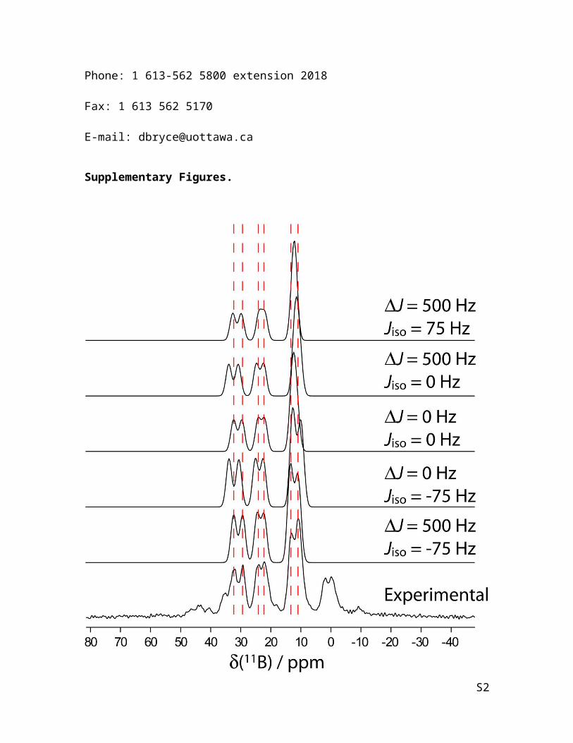
Supplementary Figures.
FIG S1. A stackplot of simulated spectra is shown for the 11B DOR NMR spectrum of 1
while including and excluding the isotropic and anisotropic J coupling. The simulations
are compared to the experimental spectrum shown in the bottom trace. The peaks near 0
ppm are spinning sidebands. B0 = 9.4 T.
S2
Page 3
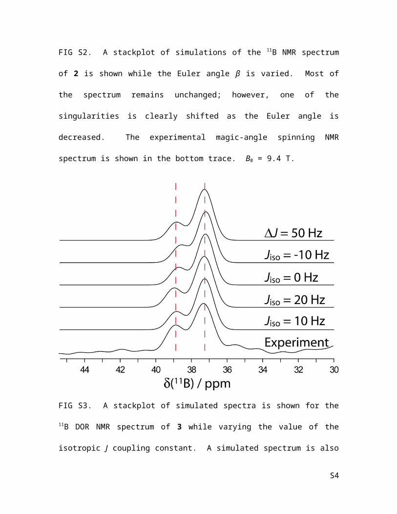
FIG S2. A stackplot of simulations of the 11B NMR spectrum of 2 is shown while the
Euler angle β is varied. Most of the spectrum remains unchanged; however, one of the
singularities is clearly shifted as the Euler angle is decreased. The experimental magic-
angle spinning NMR spectrum is shown in the bottom trace. B0 = 9.4 T.
S3
Page 4
FIG S3. A stackplot of simulated spectra is shown for the 11B DOR NMR spectrum of 3
while varying the value of the isotropic J coupling constant. A simulated spectrum is
also shown which includes some anisotropic J coupling which has little effect on the
spectrum. The experimental spectrum is shown in the bottom trace. B0 = 9.4 T.
S4
Page 5
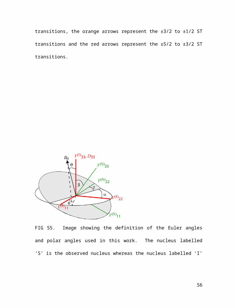
FIG S4. Energy level diagram depicting the transitions in a spin-5/2 A2 spin pair. The
blue arrows represent the CT transitions, the orange arrows represent the ±3/2 to ±1/2 ST
transitions and the red arrows represent the ±5/2 to ±3/2 ST transitions.
S5
Page 6
FIG S5. Image showing the definition of the Euler angles and polar angles used in this
work. The nucleus labelled ‘S’ is the observed nucleus whereas the nucleus labelled ‘I’ is
the perturbing nucleus. Notice that in all cases in this study, V(I)33 is always coincident
with D33.
S6
Page 7
Additional Experimental Details.
NMR Spectroscopy
Samples of B-chlorocatecholborane, 1, 4, and 5 were purchased from Aldrich and
used without further purification. Similarly, 2 was purchased from Strem and was used
without further purification. Compound 3 was prepared by reacting equimolar amounts
of sodium manganese pentacarbonyl salt and B-chlorocatecholborane in dry toluene
under an inert atmosphere using literature procedures.[1] The sodium manganese
pentacarbonyl salt was prepared by reacting 5 with a 1 % Na/Hg amalgam in dry THF.
All samples are moisture sensitive and were thus tightly packed into either vespel DOR
rotors or zirconium oxide MAS rotors under an inert atmosphere.
All DOR NMR experiments were performed at 9.4 T using a Bruker AVANCE
III console and a Bruker WB 73A DOR probe with a 14 mm outer rotor and a 4.3 mm
inner rotor. Typically, experiments were performed with the outer rotor spin rate varied
from 700 to 1000 Hz in order to identify the centerbands; the inner rotor spin rates are
typically 4 to 5 times larger and cannot be independently varied. For all experiments,
outer-rotor synchronization was used to remove the odd-ordered sidebands.[2] 20 kHz 1H
SPINAL-64 decoupling was also used for the 11B DOR NMR experiments.[3] The 11B
DOR NMR experiments were performed using 20 μs CT selective excitation pulses,
either 1 or 2 s recycle delays, and either 128 or 256 scans. The 55Mn NMR experiments
were performed using a 12.5 μs CT selective excitation pulse, 256 scans, and a 2 s
recycle delay.
The 11B MAS NMR experiments were performed at 9.4 T using a 4 mm triple
channel MAS probe, a Bruker AVANCE III spectrometer, 10 kHz MAS, a 4 s recycle
S7
Page 8
delay, and a 20 μs CT selective excitation pulse. All experiments used a rotor-
synchronized Hahn echo sequence to remove the 11B background signal from the probe.
The number of scans varied from 128 to 2560. All 11B NMR experiments were
referenced to liquid F3B·O(C2H5)2 using solid NaBH4 as a secondary reference (δ =
-42.06 ppm).
The 79/81Br NQR experiments were performed using a spin-echo sequence on a
Bruker AVANCE III spectrometer equipped with a 4 mm triple resonance MAS probe.
For the 1D experiments, the excitation pulse duration was 1 μs and the refocusing pulse
was 2 μs. The 2D nutation experiment used 512 increments of 1 μs for the first pulse
length in the spin echo experiment. The asymmetry parameter can then be determined
from the nutation powder pattern singularities as: η=3 (ν3−ν2)ν3+ν2
, where ν2 and ν3 are the
two highest-frequency singularities.[4]
The 35Cl WURST-QCPMG experiment for 2 was performed at 21.1 T using the
Bruker AVANCE II 900 NMR spectrometer at the National Ultrahigh-Field NMR
Facility for Solids in Ottawa. A two-channel 7 mm static probe was used. The
experiment used 50 μs WURST pulses sweeping 2 MHz, a 5 kHz spikelet separation, a
0.5 s recycle delay, and 4096 scans. The VOCS method was necessary and seven
subspectra were acquired with 500 kHz offsets. The chemical shifts were referenced to
dilute Cl- using solid NaCl as a secondary reference (δ = -41.11 ppm).
The 55Mn solid echo NMR spectrum was acquired at 9.4 T using a Bruker
AVANCE III spectrometer and a 4 mm triple channel MAS probe. A 1.75 μs CT
selective excitation pulse was used with a 30 μs echo delay, a 2 s recycle delay, and 200
S8
Page 9
scans. A total of 12 VOCS subspectra were acquired with 100 kHz offsets. For the 55Mn
MAS NMR experiments, the same probe was used along with 10 kHz MAS, a 2 s recycle
delay, and a 1.75 μs CT selective excitation pulse. A MAS NMR spectrum of 5 was also
collected at 21.1 T (Figure 5). A total of 128 scans were acquired at 10 kHz MAS
spinning with a 4 s recycle delay and a 1.5 μs CT selective excitation pulse. All 55Mn
NMR experiments were referenced to a 0.82 m solution of KMnO4 in D2O.
Density Functional Theory Calculations
Cluster model DFT calculations were performed using the ADF software package.[5]
For all calculations the meta-GGA functional of Tao, Perdew, Staroverov, and Scuseria
(TPSS)[6] was used along with the ZORA/QZ4P Slater-type basis sets which are core
triple-zeta, valence quadruple-zeta, and have four polarization functions.[7] The clusters
consisted of a single molecule, the coordinates of which were extracted directly from the
known crystal structures.
(GI)PAW DFT calculations of the EFG and magnetic shielding tensors were
performed using the CASTEP NMR program.[8] In all cases, a 610 eV kinetic energy
cut-off was used along with the default ‘ultra-fine’ k-point grids. On-the-fly generated
ultrasoft pseudopotentials were used on all atoms; the explicit pseudopotential strings are
given in the Supplementary Material. For all cases, the published crystal structures were
used without any modifications;[9, 10, 11, 12] in the case of 2 however, the hydrogens
needed to be added and were then subsequently optimized prior to performing the NMR
calculation. The calculated boron[13] and chlorine[14] isotropic magnetic shielding
constants were converted to chemical shifts with the use of an absolute shielding scale.
S9
Page 10
QUEST simulations
Simple, in house, modifications to the QUEST program were made in order to
calculate the resonance frequencies. Neither the Hamiltonian, Euler angles, nor the
interpolation scheme were altered for the MAS and DOR simulations. The simulations
are performed by averaging the resonance frequencies over a large number of rotor
increments. This number was systematically increased until the lineshape did not change.
The calculated lineshapes were compared to those predicted for the spin-1/2 case
implemented in WSolids when the CQ is set to zero. Although powder averaging isn’t
necessary for the DOR simulations, the interpolation scheme was still used, for
simplicity, but a powder average quality of 1 (i.e. 3 crystal orientations) was used. When
a large number of rotor increments are used in the averaging, the three calculation
resonance frequencies are degenerate and only a single, sharp, resonance is predicted.
The time necessary to calculate the DOR and MAS spectra were similar as in the latter
case no powder averaging is necessary yet a large number of rotor increments is needed.
On a laptop computer with an Intel i5 processor the calculations lasted, on average, two
seconds each. In the case of DOR NMR, only the positions of the centerbands were fit.
S10
Page 11
GIPAW DFT Pseudopotential Strings.
The following are the pseudopotential strings used for all the GIPAW DFT (CASTEP)
calculations in this work.
H 1|0.8|3.675|7.35|11.025|10UU(qc=6.4)[]
B 2|1.4|9.187|11.025|13.965|20UU:21UU(qc=5.5)[]
C 2|1.4|9.187|11.025|12.862|20UU:21UU(qc=6)[]
O 2|1.3|16.537|18.375|20.212|20UU:21UU(qc=7.5)[]
Br 2|2|2|1.4|5.6|6.6|8.8|40U=-0.74U=+0.25:41U=-0.295U=+0.25[]
N 2|1.5|11.025|12.862|14.7|20UU:21UU(qc=6)[]
Cl 2|1.7|5.88|7.35|9.187|30UU:31UU:32LGG[]
References.
S11
Page 12
1 C. S. Kraihanzel and L. G. Herman, J. Organomet. Chem. 15, 397 (1968); K. M. Waltz, X. He,
C. Muhoro, and J. F. Hartwig, J. Am. Chem. Soc. 117, 11357 (1995); K. M. Waltz, C. N.
Muhoro, and J. F. Hartwig, Organometallics, 18, 3383 (1999).
2 A. Samoson and E. Lippmaa, J. Magn. Reson, 84, 410 (1989).
3 B. M. Fung, A. K. Khitrin, and K. Ermolaev, J. Magn. Reson. 142, 97 (2000).
4 G. S. Harbison, A. Slokenbergs, and T. M. Barbara, J. Chem. Phys. 90, 5292 (1989).
5 C. F. Guerra, J. G. Snijders, G. te Velde, and E. J. Baerends, Theor. Chem. Acc. 99, 391
(1998); G. te Velde, F. M. Bickelhaupt, E. J. Baerends, C. F. Guerra, S. J. A. van Gisbergen, J.
G. Snijders, and T. Ziegler, J. Comput. Chem. 22, 931 (2001); Amsterdam Density Functional
Software ADF2009.01, SCM; Theoretical Chemistry, Vrije Universiteit: Amsterdam, the
Netherlands, 2010. <http://www.scm.com>
6 J. Tao, J. P. Perdew, V. N. Staroverov, and G. E. Scuseria, Phys. Rev. Lett. 91, 146401 (2003).
7 E. van Lenthe and E. J. Baerends, J. Comput. Chem. 24, 1142 (2003).
8 C. J. Pickard and F. Mauri, Phys. Rev. B 63, 245101 (2001); M. D. Segall, P. J. D. Lindan, M.
J. Probert, C. J. Pickard, P. J. Hasnip, S. J. Clark, and M. C. Payne, J. Phys.: Condens. Matter
14, 2717 (2002).
9 R. B. Coapes, F. E. S. Souza, M. A. Fox, A. S. Batsanov, A. E. Goeta, D. S. Yufit, M. A.
Leech, J. A. K. Howard, A. J. Scott, W. Clegg, and T. B. Marder, J. Chem. Soc., Dalton Trans.
1201 (2001).
10 D. L. Coursen and J. L. Hoard, J. Am. Chem. Soc. 74, 1742 (1952).
11 C. S. Kraihanzel and L. G. Herman, J. Organomet. Chem. 15, 397 (1968); K. M. Waltz, X. He,
C. Muhoro, and J. F. Hartwig, J. Am. Chem. Soc. 117, 11357 (1995); K. M. Waltz, C. N.
Muhoro, and J. F. Hartwig, Organometallics, 18, 3383 (1999).
12 W. Clegg, M. R. J. Elsegood, F. J. Lawlor, N. C. Norman, N. L. Pickett, E. G. Robins, A. J.
Scott, P. Nguyen, N. J. Taylor, and T. B. Marder, Inorg. Chem. 37, 5289 (1998); M. R.
Churchill, K. N. Amoh, and H. J. Wasserman, Inorg. Chem. 20, 1609 (1981).
Page 13
13 K. Jackowski, W. Makulski, A. Szyprowska, A. Antušek, M. Jaszuński, J. Jusélius, J. Chem.
Phys. 130, 044309 (2009).
14 M. Gee, R. E. Wasylishen, A. Laaksonen, J. Phys. Chem. A 103, 10805 (1999).