86
ACIL ALLEN CONSULTING REPORT TO AUSTRALIAN ENERGY MARKET OPERATOR 10 JUNE 2014 FUEL AND TECHNOLOGY COST REVIEW FINAL REPORT
A C I L A L L E N C O N S U L T I N G
REPORT TO
AUSTRALIAN ENERGY MARKET OPERATOR
10 JUNE 2014
FUEL AND TECHNOLOGY COST REVIEW
FINAL REPORT

For information on this report contact:
Owen Kelp
Principal
ACIL Allen Consulting
Ph (07) 3009 8711
Mob: 0404 811 359
Email: [email protected]
Richard Lenton
Principal
ACIL Allen Consulting
Ph (07) 3009 8713
Mob: 0404 822 316
Email: [email protected]
Gour Choudhuri Project Manager – Power Generation GHD Pty Ltd Ph (07) 3316 3442 Mob: 0407 142 840 Email: [email protected]
ACIL ALLEN CONSULTING PTY LTD
ABN 68 102 652 148
LEVEL FIFTEEN
127 CREEK STREET
BRISBANE QLD 4000
AUSTRALIA
T+61 7 3009 8700
F+61 7 3009 8799
LEVEL TWO
33 AINSLIE PLACE
CANBERRA ACT 2600
AUSTRALIA
T+61 2 6103 8200
F+61 2 6103 8233
LEVEL NINE
60 COLLINS STREET
MELBOURNE VIC 3000
AUSTRALIA
T+61 3 8650 6000
F+61 3 9654 6363
LEVEL ONE
50 PITT STREET
SYDNEY NSW 2000
AUSTRALIA
T+61 2 8272 5100
F+61 2 9247 2455
SUITE C2 CENTA BUILDING
118 RAILWAY STREET
WEST PERTH WA 6005
AUSTRALIA
T+61 8 9449 9600
F+61 8 9322 3955
ACILALLEN.COM.AU
RELIANCE AND DISCLAIMER
THE PROFESSIONAL ANALYSIS AND ADVICE IN THIS REPORT HAS BEEN PREPARED BY ACIL ALLEN CONSULTING FOR THE EXCLUSIVE USE OF THE PARTY OR PARTIES TO WHOM IT IS ADDRESSED (THE ADDRESSEE) AND FOR THE PURPOSES SPECIFIED IN IT. THIS REPORT IS SUPPLIED IN GOOD FAITH AND REFLECTS THE KNOWLEDGE, EXPERTISE AND EXPERIENCE OF THE CONSULTANTS INVOLVED. THE REPORT MUST NOT BE PUBLISHED, QUOTED OR DISSEMINATED TO ANY OTHER PARTY WITHOUT ACIL ALLEN CONSULTING’S PRIOR WRITTEN CONSENT. ACIL ALLEN CONSULTING ACCEPTS NO RESPONSIBILITY WHATSOEVER FOR ANY LOSS OCCASIONED BY ANY PERSON ACTING OR REFRAINING FROM ACTION AS A RESULT OF RELIANCE ON THE REPORT, OTHER THAN THE ADDRESSEE.
IN CONDUCTING THE ANALYSIS IN THIS REPORT ACIL ALLEN CONSULTING HAS ENDEAVOURED TO USE WHAT IT CONSIDERS IS THE BEST INFORMATION AVAILABLE AT THE DATE OF PUBLICATION, INCLUDING INFORMATION SUPPLIED BY THE ADDRESSEE. UNLESS STATED OTHERWISE, ACIL ALLEN CONSULTING DOES NOT WARRANT THE ACCURACY OF ANY FORECAST OR PROJECTION IN THE REPORT. ALTHOUGH ACIL ALLEN CONSULTING EXERCISES REASONABLE CARE WHEN MAKING FORECASTS OR PROJECTIONS, FACTORS IN THE PROCESS, SUCH AS FUTURE MARKET BEHAVIOUR, ARE INHERENTLY UNCERTAIN AND CANNOT BE FORECAST OR PROJECTED RELIABLY.
ACIL ALLEN CONSULTING SHALL NOT BE LIABLE IN RESPECT OF ANY CLAIM ARISING OUT OF THE FAILURE OF A CLIENT INVESTMENT TO PERFORM TO THE ADVANTAGE OF THE CLIENT OR TO THE ADVANTAGE OF THE CLIENT TO THE DEGREE SUGGESTED OR ASSUMED IN ANY ADVICE OR FORECAST GIVEN BY ACIL ALLEN CONSULTING.
© ACIL ALLEN CONSULTING 2014

AC I L AL L E N C O N S UL T ING
ii
C o n t e n t s 1 Introduction and background 1
2 Data deliverables 2
2.1 Format of data 2
2.2 Scope of inputs – existing generators 2
2.3 Scope of inputs – new entrants 3
3 Methodology and definitions 5
3.1 Consideration of AEMO planning scenarios 5
3.1.1 The scenarios 5
3.1.2 Scenario definitions - key parameters 10
3.2 Definitions and methodology - Existing generator costs and
parameters 11
3.2.1 Overview of methodology 11
3.2.2 Industry survey 12
3.2.3 Individual data items 12
3.3 Definitions and methodology - New entrant costs and
parameters 15
3.3.1 Overview of methodology 15
3.3.2 Scope of Estimate 16
3.3.3 Forward Curve Assumptions 17
3.3.4 Build limits 18
3.4 Emission factors 20
3.4.1 Measurement of emissions 20
3.4.2 Emission factors and intensities 20
3.4.3 Emissions scope 21
3.4.4 AEMO carbon dioxide intensity index 22
3.4.5 NGER reporting 22
3.4.6 Approach in estimating emission factors 23
3.5 Fuel costs 24
3.5.1 Contractual prices versus opportunity cost 25
3.5.2 Vertically integrated fuel supply 25
3.5.3 Projecting prices for new long-term contracts 26
4 Results – Existing generators 28
5 Results - New entrants 29

AC I L AL L E N C O N S UL T ING
iii
5.1 Introduction 29
5.2 Supercritical Pulverised Coal (PC) Technology 29
5.3 Biomass Technology 33
5.4 Gas Turbine Technology 34
5.5 Solar Photovoltaic Technologies 38
5.5.2 Dual Axis Tracking 39
5.6 Solar Thermal Technologies 41
5.6.1 Compact Linear Fresnel 41
5.6.2 Central Receiver (with Thermal Storage) 43
5.6.3 Parabolic Trough (with Thermal Storage) 45
5.6.4 Thermal Storage 47
5.6.5 Potential Improvements in CSP Technologies 48
5.6.6 Integrated Solar Combined Cycle 49
5.7 Wind Technology 51
5.7.1 Wind Resource 51
5.7.2 Typical New Entrant Size 52
5.7.3 Capital Costs Trend 52
5.7.4 Wind farm development and operational life 53
5.7.5 CAPEX Profile Assumptions (FY 2014 to FY 2040) 53
5.7.6 Operation and Maintenance Costs 54
5.8 Wave/Ocean Technology 55
5.9 Storage Technologies 56
5.9.1 Large Scale Battery Storage 56
5.9.2 Pumped Hydro Storage 57
6 Results – Gas prices 60
6.1 Approach 60
6.2 Projection results 63
7 Results – Coal prices 68
7.1 Approach 68
7.1.1 Existing power stations 68
7.1.2 New power stations 68
7.2 Export coal prices 68
7.3 Price of coal into existing power stations 70
7.4 Price of coal into new power stations by zone 77
List of boxes

AC I L AL L E N C O N S UL T ING
iv
Box 1 Types of emission factors 21
List of figures
Figure 1 Domestic inflation 7
Figure 2 Exchange rate – Euro/$A 8
Figure 3 Exchange rate – US$/$A 8
Figure 4 Export coal price (US$/tonne, nominal) 8
Figure 5 Oil price (US$/bbl, nominal) 9
Figure 6 LNG price (US$/tonne, nominal) 9
Figure 7 Steel price (US$/tonne, nominal) 9
Figure 8 Australian unemployment rate 10
Figure 9 Typical Grubb Curve 18
Figure 10 Development of gas turbine models 35
Figure 11 CLFR pilot plant at Kogan Creek 42
Figure 12 Schematics of a CSP tower system 44
Figure 13 CSP tower systems (PS10 & PS20), Seville - Spain (10 & 20MW) 44
Figure 14 A typical parabolic trough system 46
Figure 15 Schematics of CSP with thermal storage 48
Figure 16 Annual capacity factor for a 100 MW parabolic trough plant as a function of solar field size and size of thermal energy storage 48
Figure 17 Example ISCC Plant 50
Figure 18 Australian gas network representation 60
Figure 19 Projected gas prices for major load centres: Medium case 63
Figure 20 Projected gas prices (real 2014-15 $/GJ) for existing gas plant: Medium case 63
Figure 21 Projected gas prices (real 2014-15 $/GJ) for new entrants: Medium case 64
Figure 22 Projected gas prices for major load centres: High case 64
Figure 23 Projected gas prices (real 2014-15 $/GJ) for existing gas plant: High case 65
Figure 24 Projected gas prices (real 2014-15 $/GJ) for new entrants: High case 65
Figure 25 Projected gas prices for major load centres: Low case 66
Figure 26 Projected gas prices (real 2014-15 $/GJ) for existing gas plant: Low case 66
Figure 27 Projected gas prices (real 2014-15 $/GJ) for new entrants: Low case 67
Figure 28 Assumed export coal prices (Real 2014-15 A$/t) 69
Figure 29 Assumed export coal prices in comparison with historic prices 69
Figure 30 Projected coal price (real 2014-15 $/GJ) into NSW existing stations 71
Figure 31 Projected coal price (real 2014-15 $/GJ) into QLD existing stations 74
Figure 32 Projected coal price (real 2014-15 $/GJ) into VIC and SA existing stations 76
Figure 33 Coal prices into new power stations by zone (Real 2014-15 $/GJ) 78
List of tables
AC I L AL L E N C O N S UL T ING
v
Table 1 Existing generator data elements required 2
Table 2 Indicative Technology list to be examined 3
Table 3 New entrant generator data elements required 3
Table 4 Scenario definitions - Key parameters for technology and fuel costs 6
Table 5 Scenario definitions - Key parameters for technology and fuel costs 7
Table 6 Scenario definitions - Key parameters for NEM modelling 11
Table 7 Thermoflow Cost Factors (Coal) 31
Table 8 Black Coal with Carbon Capture and Storage 31
Table 9 Black Coal without Carbon Capture and Storage 32
Table 10 Brown Coal with Carbon Capture and Storage 32
Table 11 Brown Coal without Carbon Capture and Storage 33
Table 12 Biomass Technology 34
Table 13 Thermoflow Cost Factors (Gas Turbine) 36
Table 14 Combined Cycle Gas Turbine with CCS 36
Table 15 Combined Cycle Gas Turbine without CCS 37
Table 16 Open Cycle Gas Turbine 37
Table 17 PV Fixed Flat Plate/ Single Axis Tracking/ Dual Axis Tracking 40
Table 18 Compact Linear Fresnel Technology – Direct Stream Generation – No Storage 43
Table 19 Central Receiver with 6 hours thermal storage 45
Table 20 Parabolic Trough with 6 hours 47
Table 21 Integrated Solar Combined Cycle 50
Table 22 Wind 55
Table 23 Wave/Ocean 56
Table 24 Large Scale Battery Storage 57
Table 25 Pumped Storage Input Costs 58
Table 26 Pumped Hydro Storage 59
Table 27 NTNDP zone and gas market nodes 61
Table 28 NTNDP scenario assumptions 62
Table 29 Coal prices into existing power stations in NSW (Real 2014-15 $/GJ) – High scenario 72
Table 30 Coal prices into existing power stations in NSW (Real 2014-15 $/GJ) – Medium scenario 72
Table 31 Coal prices into existing power stations in NSW (Real 2014-15 $/GJ) – Low scenario 72
Table 32 Coal prices into existing power stations in Qld (Real 2014-15 $/GJ) – High scenario 75
Table 33 Coal prices into existing power stations in Qld (Real 2014-15 $/GJ) – Medium scenario 75
Table 34 Coal prices into existing power stations in Qld (Real 2014-15 $/GJ) – Low scenario 75
Table 35 Coal prices into existing power stations in Victoria and SA (Real 2014-15 $/GJ) – All scenarios 76
Table 36 Coal prices into new power stations by zone (Real 2014-15 $/GJ) – High scenario 79
Table 37 Coal prices into new power stations by zone (Real 2014-15 $/GJ) – Medium scenario 79

AC I L AL L E N C O N S UL T ING
vi
Table 38 Coal prices into new power stations by zone (Real 2014-15 $/GJ) – Low scenario 79

AC I L AL L E N C O N S UL T ING
FUEL AND TECHNOLOGY COST REVIEW FINAL REPORT 1
1 Introduction and background
The Australian Energy Market Operator’s (AEMO) planning functions rely on an underlying
set of input assumptions that characterise the behaviour of existing generation assets, and
the economics/location of future investment and retirement decisions. The dataset includes
projections of fuel and technology costs for both existing and emerging generation
technologies. The dataset also encompasses the technical operating parameters of these
units. For emerging technologies the dataset specifies location incentives/limits, construction
lead-times, and earliest commercial viability dates.
The data is used by AEMO to conduct market simulation studies for medium and long-term
planning purposes; in particular the analysis underlying the annual National Transmission
Network Development Plan (NTNDP). Emissions factor data provided/validated through this
review will also be used operationally in calculation of the Carbon Dioxide Equivalent
Intensity Index (CDEII).
ACIL Allen Consulting (ACIL Allen) have been engaged by AEMO to undertake an update of
the technology costs, fuel costs and technical parameters contained within the NTNDP
assumptions database. To assist with this review ACIL Allen has engaged GHD as a sub-
contractor to provide expert advice and estimates on new entrant technology costs,
engineering and technical matters.
This engagement requires the delivery of the analysis, recommendations for updates and
reports in stages:
The first stage of the assignment involves the review and update of Emission factors
which are used in the calculation of the CDEII. ACIL Allen has provided its assessment
and recommendations of updates to fuel emission factors in a separate report.
The second stage of the assignment was the delivery of the proposed methodology for
updating the remaining data items, which is included as Chapter 3 in this report.
Included in this chapter are the definitions and methodology employed in the estimation
of the generation cost data.
This report is one of the key deliverables of this assignment and summarises the approach
and methodology used and the key results for existing generators and new entrant
technologies. It is structured as follows:
Chapter 2 provides the scope of data elements
Chapter 3 gives an overview of the methodology and definitions used
Chapters 4 to 7 summarise the results and provide commentary for existing plant, new
entrant plant, gas prices and coal prices respectively.
A detailed dataset is provided separately as an attachment to this report, in spreadsheet
format.

AC I L AL L E N C O N S UL T ING
FUEL AND TECHNOLOGY COST REVIEW FINAL REPORT 2
2 Data deliverables
2.1 Format of data
At the completion of the assignment, the data is to be provided in the template attached to
the RFP:
on a sent-out basis using metric units
presented in real 2014-15 Australian dollars covering the period 2014-15 to 2044-45
exclusive of GST
maintaining formulas in calculated fields as much as possible.
2.2 Scope of inputs – existing generators
AEMO require data elements as shown in Table 1 on a unit basis for all scheduled and
semi-scheduled market generators. Thermal efficiency and emission factors are also
required for all non-scheduled market generators.
Table 1 Existing generator data elements required
Technical parameters
Validation of the pre-populated dataset provided by AEMO
Minimum Stable Generation (% of installed capacity)
Cold/Warm/Hot Start Notification Times (hours)
Cold/Warm/Hot Minimum Sync Times (hours)
No load fuel consumption (GJ/hour)
Auxiliary load (% of as-generated energy)
Ramp Rates (MW sent-out/hour, during standard operation and start up)
Pumping efficiency values for the pumped hydro units (energy required for pumping expressed as a %
of energy sent-out)
Thermal de-rate factors for hot climate operations (% of installed sent-out capacity)
Maintenance rate (days/year)
Full & Partial forced outage rates (on a running hours basis).
Efficiency and emission factors
Thermal Efficiency (%, HHV, sent-out and as generated)
Scope 1 Emission Factor (kg CO2e/GJ fuel)1
Scope 3 Emission Factor (kg CO2e/GJ fuel)2
Cost elements
Fixed Operating Cost ($/MW sent-out /year)
Variable Operating Cost ($/MWh sent-out)
No Load Cost ($/MW sent-out)
Cold start-up cost ($ per cold-start offline >40 hours)
Warm start-up cost ($ per warm-start — offline between 5 and 40 hours)
Hot start-up cost ($ per hot-start — offline <5 hours)
1 This data element was previously termed Combustion Emission Factor
2 The data element was previously termed Fugitive Emission Factor

AC I L AL L E N C O N S UL T ING
FUEL AND TECHNOLOGY COST REVIEW FINAL REPORT 3
Retirement / Refurbishment cost ($)
Fuel cost by year ($/GJ)
In discussions with AEMO, it was decided to remove “Minimum on/off times” from the
original scope (although ACIL Allen and GHD will attempt to estimate these values as part of
the industry survey). In addition, it was agreed that some of the ‘new’ data items such as
cold/warm/hot start notification times and costs would be undertaken by technology rather
than producing estimates for individual existing stations.
2.3 Scope of inputs – new entrants
The scope of work requires nominating the most likely generation technologies to be
commercially viable over the next 30-year period for each scenario. The RFP and template
include the technologies listed in Table 2.
Table 2 Indicative Technology list to be examined
Technology
Wind (onshore)
Biomass (with variety of fuel sources and locations)
Solar Thermal (including Compact Linear Fresnel, Parabolic Trough. Central Receiver. all with/without
6 hour storage)
Solar Photovoltaic (including Fixed Flat Plate, Single Axis Tracking and Dual Axis Tracking)
Wave/Ocean
Pumped Hydro storage
Large scale Battery storage
Integrated Solar (e.g. Kogan Creek Solar Boost - with detailed output characteristics)
Closed Cycle Gas Turbines (± Carbon Capture & Storage)
Open Cycle Gas Turbines
Super Critical Black Coal (± Carbon Capture & Storage)
Super Critical Brown Coal (± Carbon Capture & Storage)
In discussions with AEMO, it was decided to not undertake cost and parameter reviews for
geothermal, coal gasification and nuclear technologies.
The new entrant generator data elements are specified in Table 3. Where appropriate, these
should be specified for technology and region. In cases where parameters are impacted by
learning rates, the parameter should be specified separately for each year representing a
unit constructed in that year.
Table 3 New entrant generator data elements required
Technical parameters
First year assumed commercially viable (for commissioning, not construction start)
Assumed economic life (years)
Fugitive Emissions (kg CO2elGJ fuel)
Combustion Emissions (kg CO2elGJ fuel)
Emissions Capture (% of total emissions)
Assumed unit size (MW, sent-out)
Minimum Stable Generation (% of installed capacity)
Cold/Warm/Hot Start Notification Times (hours)

AC I L AL L E N C O N S UL T ING
FUEL AND TECHNOLOGY COST REVIEW FINAL REPORT 4
Cold/Warm/Hot Minimum Sync Times (hours)
No load fuel consumption (GJ/hour)
Auxiliary load (% of as—generated energy)
Ramp Rates (MW/h, during standard operation)
Thermal Efficiency (% as-generated and as sent-out, by year of construction)
Heat rate degradation curves
Pumping efficiency values for the pumped hydro units
Thermal de-rate factors for hot climate operations (% of installed sent-out capacity)
Maintenance rate (days/year)
Full & Partial forced outage rates (on a running hours basis)
Cost parameters
Fixed Operating Cost ($/MW sent-out/year)
Variable Operating Cost ($/MWh sent-out)
No Load Cost ($/MW sent-out)
Cold start-up cost ($ per cold-start offline >40 hours)
Warm start-up cost ($ per warm-start — offline between 5 and 40 hours)
Hot start-up cost ($ per hot-start - offline <5 hours)
CO2 Transport & Storage Costs by zone ($/tonne)
Fuel cost by year and by zone ($/GJ)
Capital cost by year ($/MW sent-out)
Build limits
Project lead time between construction approval and commissioning
The maximum build achievable in each zone (MW sent-out)
The maximum build rate (MW sent-out/year)
The following elements were excluded from the original scope for data item requirements on
AEMO’s advice:
Minimum on/off times
Retirement and refurbishment costs for new technologies
Contribution to peak demand for intermittent technologies.
AC I L AL L E N C O N S UL T ING
FUEL AND TECHNOLOGY COST REVIEW FINAL REPORT 5
3 Methodology and definitions
3.1 Consideration of AEMO planning scenarios
A number of the data items in the template, particularly the cost items, will vary as a function
of the three planning scenarios developed by AEMO. Therefore, a description will be
required about the way each data item varies across the scenarios. In the following chapters
while defining each data item and the methodology applied for its estimation an indication is
given as to whether it is static across the scenarios or varies with each scenario and the
approach considered for determining the variation.
3.1.1 The scenarios
The three scenarios are based on information contained in AEMO’s report titled, 2014
Planning and Forecasting Scenarios, dated 11 February 2014. AEMO commissioned
Independent Economics to produce the report titled, Economic and Energy Market
Forecasts, 9 March, which provides more detail on each scenario.
Three scenarios have been defined as part of the study and are referred to as the:
Medium centralised energy demand (Medium scenario)
High centralised energy demand (High scenario)
Low centralised energy demand (Low scenario).
Presented below are the key parameters from the scenario definitions which are relevant
when projecting the generation technology and fuel costs of the NEM.

AC I L AL L E N C O N S UL T ING
FUEL AND TECHNOLOGY COST REVIEW FINAL REPORT 6
The Independent Economics report and associated spreadsheet (provided by AEMO)
provide additional detail on each of the scenarios. ACIL Allen has extracted the relevant
details and presents them in summary form below.
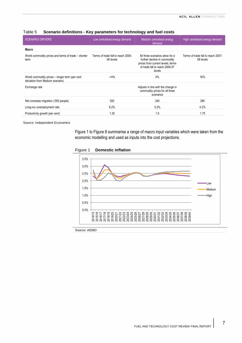
Table 4 Scenario definitions - Key parameters for technology and fuel costs
SCENARIO DRIVERS Low centralised energy demand Medium centralised energy
demand
High centralised energy demand
Energy consumption
Domestic energy consumption from centralised source
Low Medium High
Economic and demographic
Economic activity - Australian Low Medium High
Energy-intensive industrial sectors Reduced output from industrial
sectors
Continue at current levels Increased output from industrial
sectors
Population growth Low levels of economic activity and low demand for Australia’s
resources reduces requirements
for additional skilled labour and hence immigration levels are low
Central estimated growth Stronger growth to support higher economic activity
Economic activity - Global US remains weak; EU member state defaults cause new credit
freeze; slows Chinese growth
Global recovery continues Strong growth in India and China; increased growth in western
Europe and the USA
Greenhouse policy
International action on global warming NA NA NA
Carbon Implementation of Direct Action
policy in the short to medium term; coupled with safeguarding emissions reduction with a wider effect and higher strength phased
in from 2017
Implementation of Direct Action
policy in the short to medium term; coupled with safeguarding emissions reduction with a wider
effect and moderate strength
phased in from 2020
Implementation of Direct Action
policy
Renewable Energy Target Current legislation Current legislation Current legislation
SRES Current legislation Current legislation Current legislation
Domestic gas
Production Domestic gas production more difficult than in medium scenario; Australia has lower international
competitiveness
Central estimate – consistent with current growth in production
Domestic gas production higher than in medium scenario;
Australia has higher international competitiveness
Global LNG market Global LNG demand is weak Central estimate – consistent with current growth in production
Global LNG demand is strong
Penetration of gas as transport fuel Low penetration Central estimated High penetration
Technology and development
Research and development Government and industry investment in development of new
technologies is well funded and
coordinated internationally. New low-emission technologies move rapidly down their learning curve
Low, moving to moderate Investment in new technologies is constrained and slow
Distributed generation penetration (solar, cogen and
trigen)
High Moderate Low
Source: AEMO
AC I L AL L E N C O N S UL T ING
FUEL AND TECHNOLOGY COST REVIEW FINAL REPORT 7
Figure 1 to Figure 8 summarise a range of macro input variables which were taken from the
economic modelling and used as inputs into the cost projections.
Figure 1 Domestic inflation
Source: AEMO
0.0%
0.5%
1.0%
1.5%
2.0%
2.5%
3.0%
3.5%
201
4/1
5
201
5/1
6
201
6/1
7
201
7/1
8
201
8/1
9
201
9/2
0
202
0/2
1
202
1/2
2
202
2/2
3
202
3/2
4
202
4/2
5
202
5/2
6
202
6/2
7
202
7/2
8
202
8/2
9
202
9/3
0
203
0/3
1
203
1/3
2
203
2/3
3
203
3/3
4
203
4/3
5
203
5/3
6
203
6/3
7
203
7/3
8
203
8/3
9
203
9/4
0
Low
Medium
High
Table 5 Scenario definitions - Key parameters for technology and fuel costs
SCENARIO DRIVERS Low centralised energy demand Medium centralised energy
demand
High centralised energy demand
Macro
World commodity prices and terms of trade – shorter term
Terms of trade fall to reach 2005-06 levels
All three scenarios allow for a further decline in commodity
prices from current levels; terms of trade fall to reach 2006-07
levels
Terms of trade fall to reach 2007-08 levels
World commodity prices – longer term (per cent
deviation from Medium scenario)
-14% 0% 16%
Exchange rate Adjusts in line with the change in commodity prices for all three
scenarios
Net overseas migration (‘000 people) 200 240 280
Long-run unemployment rate 6.2% 5.2% 4.2%
Productivity growth (per cent) 1.25 1.5 1.75
Source: Independent Economics

AC I L AL L E N C O N S UL T ING
FUEL AND TECHNOLOGY COST REVIEW FINAL REPORT 8
Figure 2 Exchange rate – Euro/$A
Source: AEMO
Figure 3 Exchange rate – US$/$A
Source: AEMO
Figure 4 Export coal price (US$/tonne, nominal)
Source: AEMO
0.00
0.10
0.20
0.30
0.40
0.50
0.60
0.70
201
4/1
5
201
5/1
6
201
6/1
7
201
7/1
8
201
8/1
9
201
9/2
0
202
0/2
1
202
1/2
2
202
2/2
3
202
3/2
4
202
4/2
5
202
5/2
6
202
6/2
7
202
7/2
8
202
8/2
9
202
9/3
0
203
0/3
1
203
1/3
2
203
2/3
3
203
3/3
4
203
4/3
5
203
5/3
6
203
6/3
7
203
7/3
8
203
8/3
9
203
9/4
0
Low
Medium
High
0.000
0.100
0.200
0.300
0.400
0.500
0.600
0.700
0.800
0.900
201
4/1
5
201
5/1
6
201
6/1
7
201
7/1
8
201
8/1
9
201
9/2
0
202
0/2
1
202
1/2
2
202
2/2
3
202
3/2
4
202
4/2
5
202
5/2
6
202
6/2
7
202
7/2
8
202
8/2
9
202
9/3
0
203
0/3
1
203
1/3
2
203
2/3
3
203
3/3
4
203
4/3
5
203
5/3
6
203
6/3
7
203
7/3
8
203
8/3
9
203
9/4
0
Low
Medium
High
-
20.00
40.00
60.00
80.00
100.00
120.00
140.00
160.00
201
4/1
520
15/
16
201
6/1
720
17/
18
201
8/1
920
19/
20
202
0/2
120
21/
22
202
2/2
320
23/
24
202
4/2
520
25/
26
202
6/2
720
27/
28
202
8/2
920
29/
30
203
0/3
120
31/
32
203
2/3
320
33/
34
203
4/3
520
35/
36
203
6/3
720
37/
38
203
8/3
920
39/
40
Low
Medium
High

AC I L AL L E N C O N S UL T ING
FUEL AND TECHNOLOGY COST REVIEW FINAL REPORT 9
Figure 5 Oil price (US$/bbl, nominal)
Source: AEMO
Figure 6 LNG price (US$/tonne, nominal)
Source: AEMO
Figure 7 Steel price (US$/tonne, nominal)
Source: AEMO
-
20.00
40.00
60.00
80.00
100.00
120.00
140.00
160.00
180.00
201
4/1
520
15/
16
201
6/1
720
17/
18
201
8/1
920
19/
20
202
0/2
120
21/
22
202
2/2
320
23/
24
202
4/2
520
25/
26
202
6/2
720
27/
28
202
8/2
920
29/
30
203
0/3
120
31/
32
203
2/3
320
33/
34
203
4/3
520
35/
36
203
6/3
720
37/
38
203
8/3
920
39/
40
Low
Medium
High
-
200.00
400.00
600.00
800.00
1,000.00
1,200.00
201
4/1
5
201
6/1
7
201
8/1
9
202
0/2
1
202
2/2
3
202
4/2
5
202
6/2
7
202
8/2
9
203
0/3
1
203
2/3
3
203
4/3
5
203
6/3
7
203
8/3
9
Low
Medium
High
-
100.00
200.00
300.00
400.00
500.00
600.00
201
4/1
520
15/
16
201
6/1
720
17/
18
201
8/1
920
19/
20
202
0/2
120
21/
22
202
2/2
320
23/
24
202
4/2
520
25/
26
202
6/2
720
27/
28
202
8/2
920
29/
30
203
0/3
120
31/
32
203
2/3
320
33/
34
203
4/3
520
35/
36
203
6/3
720
37/
38
203
8/3
920
39/
40
Low
Medium
High

AC I L AL L E N C O N S UL T ING
FUEL AND TECHNOLOGY COST REVIEW FINAL REPORT 10
Figure 8 Australian unemployment rate
Source: AEMO
3.1.2 Scenario definitions - key parameters
Taking the above summaries, presented in the table below are the key parameters which
will influence the estimates of the data items, and a high level proposed treatment of these
parameters for the three scenarios.
0.0%
1.0%
2.0%
3.0%
4.0%
5.0%
6.0%
7.0%
201
4/1
5
201
5/1
6
201
6/1
7
201
7/1
8
201
8/1
9
201
9/2
0
202
0/2
1
202
1/2
2
202
2/2
3
202
3/2
4
202
4/2
5
202
5/2
6
202
6/2
7
202
7/2
8
202
8/2
9
202
9/3
0
203
0/3
1
203
1/3
2
203
2/3
3
203
3/3
4
203
4/3
5
203
5/3
6
203
6/3
7
203
7/3
8
203
8/3
9
203
9/4
0
Low
Medium
High

AC I L AL L E N C O N S UL T ING
FUEL AND TECHNOLOGY COST REVIEW FINAL REPORT 11
3.2 Definitions and methodology - Existing
generator costs and parameters
3.2.1 Overview of methodology
The approach adopted is a staged process which focuses on updates to the existing dataset
rather than starting from scratch.
An initial review of the data set was undertaken to assess each item and identify any
obvious changes required. These changes were initially based on in-house information and
market intelligence, acknowledging the need for transparency and a preference to rely on
publicly available data. Where possible use of publicly available data was made, including
Table 6 Scenario definitions - Key parameters for NEM modelling
Scenario parameters Data items affected Low centralised energy demand
Medium centralised energy demand
High centralised energy demand
Macro
AUD exchange rate Capital costs; export coal and LNG netback prices
As per Figure 2 and Figure 3
As per Figure 2 and Figure 3 As per Figure 2 and Figure 3
Inflation As per Figure 1 As per Figure 1 As per Figure 1
Carbon policy
International action on greenhouse emissions
Demand for energy; learning rate for emerging
technologies
Global agreement reached earlier and/or recovery in
European permit prices by 2017
Global agreement reached by 2020 and/or recovery in
European permit prices by 2020
Global agreement not reached until post 2030
and/or recovery in European permit prices by
2030
Fuel prices
Oil prices Export LNG netback prices;
cost of liquid fuels
As per Figure 5 As per Figure 5 As per Figure 5
International coal price Export coal netback prices As per Figure 4 As per Figure 4 As per Figure 4
East coast gas supply / production costs
Gas supply cost curve ACIL Allen Reference case
supply curve with low development in unconventional reserves (out of the Cooper Basin)
ACIL Allen Reference case
supply curve with moderate development in unconventional reserves (out of the Cooper Basin)
ACIL Allen Reference case
supply curve with reasonable development in unconventional reserves (out of the Cooper Basin)
Other commodity prices
Steel prices Capital costs and O&M As per Figure 7 As per Figure 7 As per Figure 7
Technology and development
Research and development Learning curve for emerging technologies
Government and industry investment in development
of new technologies is well funded and coordinated internationally. New low-emission technologies
move rapidly down their learning curve
Low, moving to moderate Investment in new technologies is constrained
and slow
Productivity growth (per cent) Learning curve for emerging technologies
1.25 1.5 1.75
Demography
Net overseas migration (‘000 people)
Labour costs – capital costs and O&M
200 240 280
Long-run unemployment rate Labour costs As per Figure 8 As per Figure 8 As per Figure 8
Source: ACIL Allen and GHD, with AEMO data
AC I L AL L E N C O N S UL T ING
FUEL AND TECHNOLOGY COST REVIEW FINAL REPORT 12
aggregate data – this often involved a degree of “forensic analysis” of indirectly observable
data (such as aggregate emissions or aggregate auxiliary loads).
After the initial review the dataset was reviewed for internal consistency by grouping stations
by technology and fuel type in order to identify any outliers. Provided an outlier can be
explained, it remained in the dataset, otherwise a change was proposed.
The proposed dataset after the initial review was presented in comparison with the original
dataset for initial feedback from AEMO.
The proposed changes were then tested within industry by way of a focused survey.
3.2.2 Industry survey
The proposed dataset was tested for reasonableness by surveying responses from industry
participants.
A “traditional” mail out or web based survey were not followed as in that case the response
rate was likely to be very low. Rather, contacts within the industry, in particular generators
were followed up directly to obtain feedback. Between the ACIL Allen and GHD team a list
of contacts was developed based on previous work undertaken for each of the generators,
and a team member was identified who is better placed to contact the potential participant.
Each survey participant was sent the proposed data set (and the existing data set) together
with a cover letter explaining the process before personal contact was made.
Upon completion of the survey the team compiled a list of proposed changes to the dataset,
citing reasons at a high level and prepared a high level summary of the degree of
agreement. This was then presented to AEMO for feedback.
Given the potential confidential nature of the feedback, only a very high level summary is
provided in this report.
The industry survey was limited to the list of scheduled and semi-scheduled stations.
3.2.3 Individual data items
The following definitions were included in the survey cover letter.
Minimum stable load
Minimum stable load (or MinGen) is a measure of the lower bound that the generator unit
can be dispatched at any instant while maintaining a stable combustion process. Minimum
stable loads vary across each generator as a function of technology, fuel type and location.
The usual way of expressing the station minimum stable load is in percentage form and
when applied to the gross capacity.
Minimum On/Off Times
Minimum time, in hours, a given unit can be dispatched or turned-off within the simulation
modelling.
Cold/Warm/Hot Start Notification and Minimum Sync Times
Notification time is a measure of time in hours required to mobilise the appropriate
resources for a unit start up or first firing.
Minimum Sync time is the synchronisation time in hours required from first firing to
synchronise the unit to the national electricity grid and being ready to accept load.

AC I L AL L E N C O N S UL T ING
FUEL AND TECHNOLOGY COST REVIEW FINAL REPORT 13
Auxiliary load
Auxiliary load is an electricity load used within a power station as part of the electricity
generation process – that is, it is an electricity load used in the making of electricity (also
called a parasitic load). The usual way of expressing the station auxiliaries is in percentage
form and when applied to the gross capacity of the station provides a measure of the net
capacity or sent-out capacity of the station.
Station auxiliaries also impact the sent-out or net thermal efficiency of the station, and
therefore the station’s SRMC.
Ramp Rates
Ramp rate refers to a change in generation output over a given unit of time, and describes
the ability of a generating unit to change its output. Technically, ramp rates are usually
expressed in MW per minute, but given the ramp rates are likely to be used in modelling the
market at an hourly resolution, AEMO require them to be estimated in MW per hour. AEMO
also require a ramp up and a ramp down rate.
Thermal efficiency
Thermal efficiency is presented on a HHV sent-out basis (in GJ/MWh).
Pumping efficiency
Pumping efficiency for the pumped storage hydro units is a measure of the energy required
to pump a given volume of water from the lower reservoir to the upper reservoir compared
with the energy generated when that same volume of water is released from the upper
reservoir via the turbines to the lower reservoir.
Thermal de-rate factors for hot climate operations
Thermal de-rate factors are a measure of a station’s maximum available capacity during
periods of high ambient temperature relative to its maximum available capacity during
normal ambient conditions.
AEMO has provided the following temperature cut-offs which are consistent with the
generators’ survey:
Queensland - 37°C
NSW - 42°C
Victoria - 41°C
South Australia - 43°C
Tasmania – 1.2°C.
Note that Tasmania is more affected by winter temperature than summer and the de-rate
factor is therefore related to temperatures at 1.2 °C
Planned and Maintenance Outage rate
The planned and maintenance outage rate defines the amount of time each generator unit is
off-line for planned or maintenance outages in a given year. A planned outage (full or partial)
is an outage that has been anticipated well in advance, even if the timing plan has changed.

AC I L AL L E N C O N S UL T ING
FUEL AND TECHNOLOGY COST REVIEW FINAL REPORT 14
Maintenance Outages are not forced or planned outages. A maintenance outage refers to
an outage that has not been anticipated well in advance, but could have been deferred or
the unit being maintained recalled had there been a commercial driver to do so3.
In reality, the rate varies year by year, normally in the form of a planned maintenance cycle
– consisting of major and minor maintenance periods. However, a single/static value is
required by AEMO and therefore will be an average rate across the remaining life of each
asset. The value is to be expressed in days per year.
Full & Partial forced outage rates (on a running hours basis)
Full and partial forced outage rates represent the percent of time within a year the plant is
unavailable due to circumstances other than a planned and maintenance event. Forced
outages are not planned or maintenance outages. In principle, “forced outages” represent
the risk that a unit’s capacity will be affected by limitations beyond a generator’s control. An
outage (including full outage, partial outage or a failed start) is considered “forced” if the
outage cannot reasonably be delayed beyond 48 hours4.
It will be important to properly account (or discount) unusual events such coal supply
constraints when assessing the forced outage rates.
Fixed Operating Cost
Fixed O&M costs ($/MW/year) represent the costs of operation and maintenance that do not
vary with output, such as wages and salaries, insurances, other overheads and periodic
maintenance. For stations that are vertically integrated with their fuel supply, fixed O&M
costs can also include fixed costs associated with the coal mine/gas field.
Variable Operating Cost
The additional operating and maintenance costs for an increment of electrical output depend
on a number of factors, including the size of the increment in generation, the way in which
wear and tear on the generation units is accrued between scheduled maintenance (hours
running or a specific number of start-stop cycles) and whether operation is as a base load or
peaking facility. Generally, variable O&M is a relatively small portion of the overall SRMC for
fossil fuel fired power plants.
For coal, variable O&M includes additional consumables such as water, chemicals and
energy used in auxiliaries including incremental running costs for coal and ash handling etc.
For gas, in addition to consumables and additional operating costs, an allowance is also
included for major maintenance. The reason for including an allowance for major
maintenance in the variable O&M for gas turbines is because this maintenance is not
periodic, as it is for coal plant, but rather is generally determined by hours of operation and
often in addition is related to the number of specific events such as starts, stops, trips etc.
The OCGT peaking plant will have higher variable O&M per MWh than a CCGT base or
intermediate load plant for following reasons:
The OCGT plants will have more number of start/stops and part load operation than
CCGT plants and
3 See AEMO’s GUIDEBOOK FOR FORCED OUTAGE DATA RECORDING: DEFINITIONS AND ASSUMPTIONS
http://www.aemo.com.au/Electricity/Policies-and-Procedures/Reserve-Management/Forced-Outage-Data-Working-Group
4 Ibid

AC I L AL L E N C O N S UL T ING
FUEL AND TECHNOLOGY COST REVIEW FINAL REPORT 15
The output from gas turbine is about two third of the CCGT plant output. The steam
turbine maintenance costs are generally lower as compared to gas turbine maintenance
costs.
The variable O&M value is usually expressed in sent-out terms to account for internal usage
by the station (see below) rather than in ‘as generated’ terms.
No load fuel consumption
No load fuel consumption is the quantity of primary and secondary fuel being consumed
when the unit is synchronised to the grid but not despatching any load to the grid other than
generation of the house load or the plant auxiliary load to be expressed as GJ/hour for each
type of fuel such as primary and secondary fuel either independently or together.
No Load Cost
For no load costs ($/MW), estimates will be developed based on technology, fuel and
specific application. The No Load Cost is the cost of not running a station for an extended
period of time (the operation at Gladstone which generally results in the operation of five out
six units is a current example). This approach still requires maintenance but is much less
costly than the fixed maintenance (FOM) needed for a unit which is running.
No Load Cost is not to be confused with No load fuel consumption which relates to shorter
term fuel costs associated with the unit being synchronised to the grid but not despatching
load.
Start-up costs
The start-up costs will include plant maintenance cost, the fuel cost and any other
identifiable cost related to the plant start-up.
Retirement / Rehabilitation cost
This cost shall include the cost of end of life plant remediation and site rehabilitation. These
costs are often plant and technology specific and are significantly influenced by local
statutory rules and regulations and the provisions under the development approval.
Fuel costs
The study approach in providing updated fuel cost estimates is reported separately in
Chapter 3.5.
3.3 Definitions and methodology - New entrant
costs and parameters
3.3.1 Overview of methodology
Similar to the data items for the existing generators, this study proposed approach is a
staged process which focuses on updates to the existing dataset rather than starting from
scratch.
To review and develop current costs for respective generation technologies, a variety of cost
estimating methodologies were employed including:
Compilation of data available in the public domain,
Benchmarking against recent project costs (where available)

AC I L AL L E N C O N S UL T ING
FUEL AND TECHNOLOGY COST REVIEW FINAL REPORT 16
New coal fired power, CCGT/OCGT and biomass cost estimates based on Thermoflow
software GTPro, GTMaster, SteamPro, SteamMaster and PEACE. This software models
plant performance and provides Engineering, Procurement and Construction (EPC) and
total project cost data.
Industry suppliers regularly update performance and costing information to
Thermoflow
Cost factors are built into the software for modelling to Australian conditions such as
foreign exchange, materials and labour cost
Development of cost and performance adjustment factors for application to new plant
sourced from Asian continent reflecting Australia’s increasing comfort with equipment
from these sources and its maturing delivery standards.
Future trends – based on OEM information, industry analysis papers and GHD internal
data
Renewables – direct experience in projects, surveys of vendors’ products, access to
industry association papers and public domain material.
3.3.2 Scope of Estimate
All estimates are based on a complete power plant facility on a generic site.
An EPC contracting strategy has been assumed where the EPC scope is conducted by a
main contractor with multiple subcontracts working under the main contractor. This standard
contracting strategy provides a high degree of certainty of costs for the facility but
traditionally attracts risk premiums built into the EPC price.
No site specific conditions have been considered in the estimates.
Labour costs are based on 2014/15 Australian Rates and productivities in a competitive
bidding environment.
Direct Cost Estimates
Estimated direct costs for new generation facilities include costs for all major plant,
materials, minor equipment and labour involved in the development of the power plant to
commercial operation.
Indirect Cost Estimates
Estimated indirect costs for new generation include all owner’s costs to cover expenses
leading up to commencing construction and anything not covered under an EPC contract
during construction. Specific development cost items which have been estimated or
assumed are listed below:
Concept/Feasibility Studies and Project Development
Site acquisition
Legal fees
Project support team
Development approvals
Duties and taxes
Operator training
Commissioning and testing (including fuel).

AC I L AL L E N C O N S UL T ING
FUEL AND TECHNOLOGY COST REVIEW FINAL REPORT 17
Exclusions
The following items are excluded from the direct and indirect capital costs:
Costs of electricity network augmentation required to connect the generator to the NEM
Escalation throughout the period-of-performance
All taxes
Site specific considerations including but not limited to: seismic zone, accessibility, local
regulatory requirements, excessive rock, piles, lay down space, etc.
For CCS cases, the cost associated for CO2 injection wells, pipelines to deliver the CO2
from the power plant to the storage facility and all administration supervision and control
costs for the facility
Import tariffs that may be charged for importing equipment to Australia or shipping
charges for this equipment, and
Interest during construction and financing costs.
3.3.3 Forward Curve Assumptions
Forward cost curves are based on AEMO’s Economic and Energy Market Forecasts 2014
report by Independent Economics.
Exchange Rate
The exchange rate assumptions from the scenario definitions will be adopted.
Productivity Rate
One of the key assumptions used in the development of economic scenarios in AEMO’s
Economic and Energy Market Forecasts 2014 report by Independent Economics is
productivity growth.
The medium scenario’s productivity growth rate of 1.5% matches average growth over the
last 20 years.
Commodity Variation
Another of the key assumptions used in the development of economic scenarios in AEMO’s
Economic and Energy Market Forecasts 2014 report by Independent Economics is
commodity variation.
Technological Improvement
Pricing trends due to technological improvements over the next 30 years are likely to be one
of the most significant factors for cost estimation.
Generally, assumptions have been made based on the expected trend for each technology
following a typical Grubb curve shown in Figure 9. Each technology is assumed at a specific
point of the curve according to the level of maturity for that technology.

AC I L AL L E N C O N S UL T ING
FUEL AND TECHNOLOGY COST REVIEW FINAL REPORT 18
Figure 9 Typical Grubb Curve
Source: GHD – taken from EPRI (2010)
3.3.4 Build limits
Build limits include:
project lead time (by technology)
maximum build achievable (by technology and zone)
maximum build rate (by technology)
The analysis will build on the assumptions of the 2012 WorleyParsons report which defined
the regional annual build limit as the physical ability to deliver a project as opposed to the
ability to establish a commercial case to progress a project.
The principal influencing factors which impact the annual build capacity across all
technologies (in addition to some individual technology specific factors) will include:
The ability to source plant and equipment
The ability to source sufficient general and specialised labour to construct the plant
The ability to source necessary specialised equipment for construction of the plant
The ability to source sufficient fuel feedstock to supply the planned plant
The ability to source water
The availability of sufficient electricity network infrastructure to export planned
generation capacity
Permitting constraints.
Individual issues which apply to specific technologies, e.g. availability of carbon storage
reservoirs for CCS and acceptable penetration of variable (non-scheduled) generation into
the network shall be considered.
Ability to Source Plant and Equipment
The majority of specialised components for all of the generation categories are
manufactured internationally for Australian projects. This is expected to continue to be the
case for the forecast period. The demand for equipment in Australia is unlikely to comprise a
significant proportion of the manufacturing capacity, thus variation in Australian demand in
isolation is unlikely to have a significant impact on the supply of plant and equipment.

AC I L AL L E N C O N S UL T ING
FUEL AND TECHNOLOGY COST REVIEW FINAL REPORT 19
Significant variation in international demand for specific technology may have an impact on
the supply to Australia, however, such future constraints are difficult to forecast.
Therefore, it is assumed that constraints on the ability to source specialised plant and
equipment are unlikely to contribute significantly to regional annual build limits.
Ability to Source Labour
Although the Australian market is currently experiencing a slowing level of economic activity
in the resources sector, skilled labour constraints continue to be considered present in the
Australian economy. This constraint is particularly accentuated in the mineral rich and more
remote parts of the country. Such skilled labour shortages are often cyclic and dependent
on the general growth patterns in the broader global economy.
The impact of a slowing global economy on the capital cost for delivery of projects has been
considered; new projects are expected to maintain a higher cost to deliver, though not
necessarily causing a constraint on the annual build limit.
Ability to Source Specialised Construction Equipment
The delivery of some large scale generation projects may require the use of specialised
construction equipment.
It is not considered that constraints around sourcing specialised equipment will impact the
regional annual build, but rather, as with the discussion on labour, may have an impact on
the cost to deliver the projects.
Ability to Supply Fuel Feedstock
This analysis assumes the planned development of new generation capacity is based on the
availability of sufficient and viable fuel supply. Constraints in infrastructure to supply the fuel
to the generation plant may impact on the ability to deliver a project, however, solutions to
fuel supply constraints are assumed to be incorporated into the development of a new
generation project.
Ability to Source Water
Regional availability of water, both now and into the future, is likely to impact on the annual
build limits for particular technology types. Where water is currently in short supply, or may
become scarcer, it is likely that the application of wet cooled thermal generation
technologies may be limited and air cooling would be preferable.
Availability of Electricity Network Infrastructure
One of the primary constraints on development of projects in a region is the availability of
sufficient network capacity to effectively deliver the generation to the load taking into
account the time required to plan, approve and build new powerlines. As with the impact of
fuel supply, solutions to network constraints are assumed to be incorporated into the
development of a new generation project, and thus not considered a separate factor limiting
the regional annual build limit.
Permitting Constraints
Constraints on permitting for new build generation capacity can result from a number of
factors including social acceptance of development, policy and legislative requirements and
a capacity to process approvals. Such constraints can have a significant impact on the
AC I L AL L E N C O N S UL T ING
FUEL AND TECHNOLOGY COST REVIEW FINAL REPORT 20
timeframe to deliver a project, and thus the annual build will be limited by the ability to clear
necessary permitting steps in development.
Necessary permitting will also be influenced by government policy, both at a State and
Federal level. While the ability to deliver projects and associated approval timeframes can
be estimated under present policy settings, future changes to policy can have an impact on
the delivery time and the annual build limits.
Technology Specific Constraints
In addition to the principal factors impacting the annual build limit as outlined above, there
are a number of factors specific to technologies that will impact the ability to deliver projects
in a specific region.
These will include:
CCS: The availability to access appropriate storage structures at an economic cost.
Wind: Ability to access land with an appropriate wind resource in a specific region. This
can be influenced by both the topography and the division of land and population
density.
Wind/Solar: penetration of non-scheduled and semi-scheduled generation into the
network. There are a number of studies suggesting that at penetration levels above 25 to
30%, the cost to integrate additional non-scheduled variable generation into the network,
can increase. The extent to which this will be a regional constraint will depend on the
future connection infrastructure and systems operational regimes.
3.4 Emission factors
This section outlines the approach in estimating the emission factors for each scheduled,
semi-scheduled and non-scheduled generator in the NEM.
3.4.1 Measurement of emissions
Greenhouse gas emissions are measured in carbon dioxide equivalence (CO2-e). These are
comprised of the following emissions to the atmosphere:
carbon dioxide (CO2)
methane (CH4)
nitrous oxide (N2O), or
perfluorocarbons specified in the NGER Regulations and that are attributable to
aluminium production.
The equivalence measure allows the global warming potential of each greenhouse gas to be
standardised relative to carbon dioxide.
3.4.2 Emission factors and intensities
In the context of an electricity generator an Emission factor relates the amount of
greenhouse gas emitted per unit of fuel consumed (expressed in units of CO2-e per unit of
fuel consumed).
When combined with the power stations’ thermal efficiency, one can calculate the
Emissions intensity of the station, expressed in unit of CO2-e per unit of electricity
produced (either sent-out or as generated).

AC I L AL L E N C O N S UL T ING
FUEL AND TECHNOLOGY COST REVIEW FINAL REPORT 21
For the purpose of this work, we have been tasked with providing estimates of stations
emission factors and thermal efficiencies separately. This allows AEMO to calculate
emission intensity values for each power station.
Note that these definitions align with the NGA Factors workbook which provides estimates of
Emission factors for various fuel types in kg CO2-e/GJ.
In contrast, AEMO in its procedure for calculation of the Carbon Dioxide Equivalent Intensity
Index5 refer to Emission factors as being both defined on a per GJ and on a per MWh basis.
3.4.3 Emissions scope
In the language of carbon accounting, for example as set out in the Australian Government’s
National Greenhouse Accounts (NGA) Factors publications, there are a number of different
emission ‘scopes’. These are defined in Box 1.
Box 1 Types of emission factors
Firstly, it is important to note that an emission factor is activity-specific. The activity determines the emission factor used. The scope that emissions are reported under is determined by whether the activity is within the organisation’s boundary (direct—scope 1) or outside it (indirect—scope 2 and scope 3).
Direct (or point-source) emission factors give the kilograms of carbon dioxide equivalent (CO2-e) emitted per unit of activity at the point of emission release (i.e. fuel use, energy use, manufacturing process activity, mining activity, on-site waste disposal, etc.). These factors are used to calculate scope 1 emissions.
Indirect emission factors are used to calculate scope 2 emissions from the generation of the electricity purchased and consumed by an organisation as kilograms of CO2-e per unit of electricity consumed. Scope 2 emissions are physically produced by the burning of fuels (coal, natural gas, etc.) at the power station.
Various emission factors can be used to calculate scope 3 emissions. For ease of use, this workbook reports specific ‘scope 3’ emission factors for organisations that:
a) burn fossil fuels: to estimate their indirect emissions attributable to the extraction, production and transport of those fuels; or
b) consume purchased electricity: to estimate their indirect emissions from the extraction, production and transport of fuel burned at generation and the indirect emissions attributable to the electricity lost in delivery in the transmission and distribution network.
Source: Department of Industry, Innovation, Climate Change, Science, Research and Tertiary Education, Australian National Greenhouse Accounts: National Greenhouse Accounts Factors, July 2013, p7
In simple terms for electricity generators:
Scope 1 emissions relate to emissions associated with combustion of fuels on-site or
other emissions associated with the power station facility
Scope 2 emissions relate to indirect emissions from any electricity purchased from the
grid
Scope 3 relate to indirect emissions associated with the extraction, production and
transport of fuel to the power station.
It should be recognised that this definition does cause an issue for renewable generators
which do not consume fossil fuel in generating electricity, despite some of these entities
5 AEMO, Carbon Dioxide Equivalent Intensity Index Procedure, August 2013
AC I L AL L E N C O N S UL T ING
FUEL AND TECHNOLOGY COST REVIEW FINAL REPORT 22
reporting scope 1 emissions under the NGER scheme. For renewable plant an Emission
factor of zero will be set, despite them possibly having a non-zero Emission intensity value.6
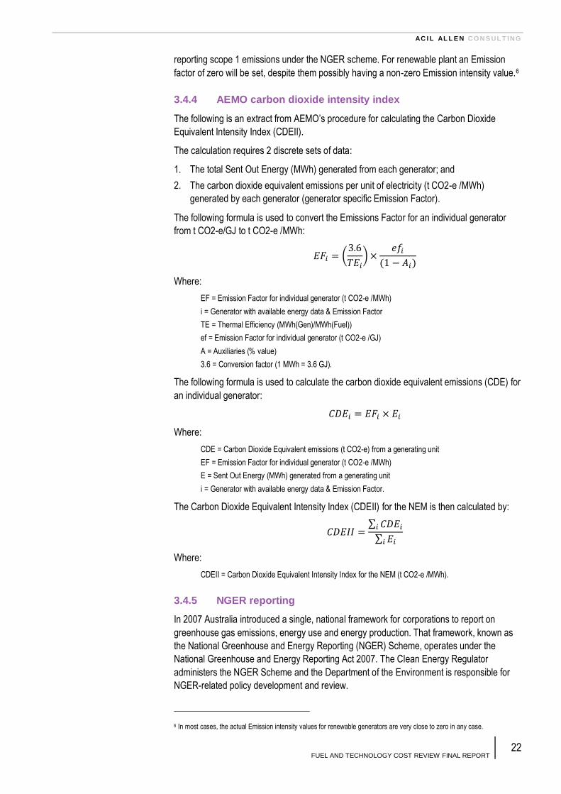
3.4.4 AEMO carbon dioxide intensity index
The following is an extract from AEMO’s procedure for calculating the Carbon Dioxide
Equivalent Intensity Index (CDEII).
The calculation requires 2 discrete sets of data:
1. The total Sent Out Energy (MWh) generated from each generator; and
2. The carbon dioxide equivalent emissions per unit of electricity (t CO2-e /MWh)
generated by each generator (generator specific Emission Factor).
The following formula is used to convert the Emissions Factor for an individual generator
from t CO2-e/GJ to t CO2-e /MWh:
(
)
Where:
EF = Emission Factor for individual generator (t CO2-e /MWh)
i = Generator with available energy data & Emission Factor
TE = Thermal Efficiency (MWh(Gen)/MWh(Fuel))
ef = Emission Factor for individual generator (t CO2-e /GJ)
A = Auxiliaries (% value)
3.6 = Conversion factor (1 MWh = 3.6 GJ).
The following formula is used to calculate the carbon dioxide equivalent emissions (CDE) for
an individual generator:
Where:
CDE = Carbon Dioxide Equivalent emissions (t CO2-e) from a generating unit
EF = Emission Factor for individual generator (t CO2-e /MWh)
E = Sent Out Energy (MWh) generated from a generating unit
i = Generator with available energy data & Emission Factor.
The Carbon Dioxide Equivalent Intensity Index (CDEII) for the NEM is then calculated by:
∑
∑
Where:
CDEII = Carbon Dioxide Equivalent Intensity Index for the NEM (t CO2-e /MWh).
3.4.5 NGER reporting
In 2007 Australia introduced a single, national framework for corporations to report on
greenhouse gas emissions, energy use and energy production. That framework, known as
the National Greenhouse and Energy Reporting (NGER) Scheme, operates under the
National Greenhouse and Energy Reporting Act 2007. The Clean Energy Regulator
administers the NGER Scheme and the Department of the Environment is responsible for
NGER-related policy development and review.
6 In most cases, the actual Emission intensity values for renewable generators are very close to zero in any case.

AC I L AL L E N C O N S UL T ING
FUEL AND TECHNOLOGY COST REVIEW FINAL REPORT 23
Under the NGER Scheme, companies which meet the threshold criteria7 are required to
report annually ‘Scope 1’ emissions, ‘Scope 2’ emissions, energy production and energy
consumption.
The National Greenhouse and Energy Reporting Regulations 2008 define ‘Scope 1’ and
‘Scope 2’ emissions as follows:
‘Scope 1’ emission of greenhouse gas, in relation to a facility, means the release of greenhouse
gas into the atmosphere as a direct result of an activity or series of activities (including ancillary
activities) that constitute the facility.
‘Scope 2’ emission of greenhouse gas, in relation to a facility, means the release of greenhouse
gas into the atmosphere as a direct result of one or more activities that generate electricity,
heating, cooling or steam that is consumed by the facility but that do not form part of the facility.
For electricity generators, ‘Scope 1’ emissions generally relate to greenhouse gas emissions
associated with combustion of fuel in the electricity generation process. ‘Scope 2’ emissions
would also accrue due to any purchased electricity sourced from the grid or from heat/steam
acquired from an external source which is then used to generate electricity by the facility.
It is important to note that under the Clean Energy Act 2011, liability for covered emissions
only include ‘Scope 1’ emissions under the carbon pricing mechanism. Entities are not liable
for 'Scope 2' emissions.
For the reporting year 2012-13, the Clean Energy Regulator has for the first time made
public reported energy production and scope 1 & 2 emission values at facility level.8
Information reported by designated generation facilities is published for facilities where the
principal activity is electricity generation and where the facility is not part of a vertically-
integrated production process. Facilities generating electricity for their own use or as a
secondary activity do not have their emissions and electricity production data published.
3.4.6 Approach in estimating emission factors
The proposed approach in estimating emission factors for this exercise is as follows:
1. Review CER data for NEM market generators (scheduled, semi-scheduled and non-
scheduled generators)
2. Verify the basis of the Electricity Production (GJ) value in the CER data (i.e. whether it’s
sent-out or as generated). This should be obtainable from the NGERs Act and/or
reporting guidelines for companies published by the CER
3. From this data, calculate Emission intensity values for each generator based on Scope
1 emissions only on a tonnes CO2-e/MWh sent-out basis
4. Calculate Emission intensity values from existing AEMO NTNDP input assumptions
(using the emission factors termed ‘Combustion’ only as the CER values do not contain
Scope 3 components)
5. Calculate Emission intensity values from current ACIL Allen internal database values
6. Undertake a comparison of the actual CER values obtained against existing NTNDP
and ACIL Allen estimates and between like for like plant.
7. Consider the plants running regime and other operational parameters (such as coal
quality) through 2012-13 a decide whether this represents its typical running state
7 The threshold criteria at facility level are currently set at 25 kt CO2-e or more of greenhouse gases; production of 100 TJ or
more of energy, or consumption of 100 TJ or more of energy. Corporate facility thresholds also apply for aggregate volumes of 50 kt CO2-e or more of greenhouse gases; production of 200 TJ or more of energy or consumption of 200 TJ or
more of energy.
8 See http://www.cleanenergyregulator.gov.au/National-Greenhouse-and-Energy-Reporting/published-information/greenhouse-and-energy-information/Greenhouse-and-Energy-information-2012-2013/Pages/default.aspx
AC I L AL L E N C O N S UL T ING
FUEL AND TECHNOLOGY COST REVIEW FINAL REPORT 24
8. Settle on any appropriate adjustments to existing values and clearly state the rationale
for the proposed change.
This will result in a recommended Emissions intensity value (Scope 1 only) for each
generator (in tonnes CO2-e/MWh either sent-out or as-generated depending upon result of
Step 2 above).
To this an estimate of the Scope 3 emission intensity values (to be estimated separately
based on non-CER data) may be added to yield a Scope 1 & 3 Emission intensity value
which corresponds with the current values used in the CDEII. Scope 3 values will principally
be sourced from the NGA factors workbook (July 2013)9.
This approach essentially involves estimating the final Emission intensity figure, rather than
its component parts which make up the calculation. This allows to modify thermal
efficiencies, emission factors (and auxiliary use factors if relevant) at a later stage in the
project, with the overall constraint being that the Emission intensity value matches those set
in this early stage.
It is noted that AEMO’s emission factors as used in the CDEII use the sum of ‘Combustion’
emission factors and ‘Fugitive’ emission factors in the calculation of the index. It is proposed
to amend the terms used as follows:
Replace ‘Combustion’ emission factor with ‘Scope 1’ emission factor. This is a more
correct term as liability for emissions from a facility can relate to more than combustion
of fossil fuels in the generation process (e.g. wind farms report a small amount of scope
1 emissions presumably due to vehicle use or other ancillary operations associated with
the farm)
Replace ‘Fugitive’ emission factor with ‘Scope 3’ emission factor. This is also a more
correct term as Fugitive emissions solely relate to unintended leakages. The term
‘Scope 3’ emissions on the other hand, include all emissions associated with the
extraction, production and transport of fuels to the power station which is the intended
purpose of the measure.
Whilst inclusion of the Scope 3 emission factors is useful when conducting market modelling
(it saves amending fuel price series each time the carbon price changes), in ACIL Allen’s
opinion, it is not a useful measure for estimating emissions from the electricity sector. Scope
3 emissions occur elsewhere throughout Australia and potentially even overseas when
imported fuels are used (e.g. diesel). It also overstates the direct carbon emission liability for
generators as they are only liable to pay for Scope 1 emissions. However considerations of
modification to the CDEII are outside our scope of work and are mentioned here only for
discussion purposes.
3.5 Fuel costs
ACIL Allen maintains a database of existing fuel supply contracts (in terms of volumes,
terms and prices) based on publicly available information. This database has been used as
a starting point for estimating fuel costs.
Projections of fuel costs beyond existing contracts is developed by using in house gas and
coal models, taking into account the different scenario definitions.
9 Department of Industry, Innovation, Climate Change, Science, Research and Tertiary Education, Australian National
Greenhouse Accounts: National Greenhouse Accounts Factors, July 2013

AC I L AL L E N C O N S UL T ING
FUEL AND TECHNOLOGY COST REVIEW FINAL REPORT 25
A number of parameters are required to ensure proper description of each scenario in these
models, and AEMO is provided with these key assumptions to ensure these are internally
consistent with each scenario definition.
The marginal fuel cost to a station is dependent on a number of factors including:
• Contractual arrangements including pricing, indexation, tenure and take or pay
provisions
• Mine/gas field and power station ownership arrangements
• Availability of fuel through spot purchases or valuation on an opportunity cost basis
• Projected prices for new long-term contracts.
Each of these factors is taken into account in evaluating the fuel cost component. The
factors are discussed below.
3.5.1 Contractual prices versus opportunity cost
Where the power station is dependent on a third party to supply fuel under contract then the
cost of incremental fuel within the AEMO dataset has historically been the average contract
price on a delivered basis.
In some cases this is still the relevant value; however the divergence between legacy
contract prices and current market prices has grown significantly for both coal and gas. In
some cases generators no longer consider prices under existing contracts to be their
marginal cost of fuel, but rather look to the opportunity cost of the commodity. This is
illustrated by the recent decision by Stanwell to sell contracted gas to other users rather
than utilise it at Swanbank E. If the gas or coal has a higher value elsewhere and on-sale is
feasible then this should represent the marginal fuel cost.
ACIL Allen will examine the fuel supply situation for each station individually and make a
judgement about whether legacy contract prices or opportunity value is the more appropriate
value. The may vary across the scenario definitions if the spread in commodity prices is
large.
3.5.2 Vertically integrated fuel supply
Stations which are fully vertically integrated with their fuel supply have lower fuel costs as a
small increment in fuel use is unlikely to require additional capital and maintenance and
hence this incremental fuel does not include these costs. Most brown coal stations in
Victoria fall into this category (incremental fuel costs are reduced to marginal diesel and
electricity costs from mining another tonne of coal).
For station owners who also own the associated coal mine and deposit but use contract
miners, the marginal fuel cost will be dependent on the contractual arrangements with the
contract miner and may not reflect the marginal cost if mining activities were carried out in-
house. For stations such as these, the estimated mining contractor costs are used as the
marginal cost of fuel.
Importantly, most vertically integrated fuel/power station developments do not have ready
access to export markets/alternative buyers and therefore the true economic opportunity
cost of fuel generally is the incremental cost of production. For those that could conceivably
access alternative markets, an opportunity cost value will be considered.

AC I L AL L E N C O N S UL T ING
FUEL AND TECHNOLOGY COST REVIEW FINAL REPORT 26
3.5.3 Projecting prices for new long-term contracts
The following section outlines the proposed approach in projecting fuel prices for new long-
term contracts. Coal, natural gas and liquid fuels are discussed separately.
Black coal – NSW and Queensland
New long-term coal prices for particular deposits depend upon the cost of mining and
preparation (if required), whether the coal is of suitable quality and can access export
markets. Other factors include ownership/vertical integration (for mine mouth developments)
and transportation costs.
Analysis of coal prices relies principally upon estimates of costs of production and transport
(if relevant) to the station in question. This analysis is undertaken on a deposit-by-deposit
basis and takes into consideration the coal resources available.
Where coal is exportable, the netback price available for the coal producer becomes a factor
in considering prices potentially available for power generation. However, given the stability
offered from domestic contracts, which offer long-terms at fixed prices, we assume that
domestic coal receive a 20% discount over the export parity value of the Run-of-Mine
(ROM) coal. ACIL Allen will incorporate the projected thermal coal export price from the
economic modelling of the three scenarios.
Hence the projected coal prices for new contracts for each NEM zone will be one of three
values:
• 80% of the export parity value of the ROM coal where it is greater than the ROM coal
mining cost. This generally applies to deposits which are higher quality coal and/or are
generally closer to the export terminals.
• ROM coal mining costs where 80% of the export parity value of the ROM coal is less
than the mining costs and the coal is delivered to a mine-mouth power station. This
usually applies to deposits which are relatively inferior in quality and/or some distance
from export terminals while being relatively close to major transmission links (Felton,
New Acland, Ulan etc).
• ROM coal mining costs plus transport costs to a power station site remote from the
mine but closer to transmission infrastructure and where 80% export parity value of the
ROM coal is again less than the mining costs but where the deposit is greater than
100 km from the transmission system (Wandoan, Alpha, Pentland).
The delivered prices can switch from one basis to another as export prices and ROM coal
mining costs are projected to vary. This is particularly the case where export prices are
projected to fall in real terms while mining costs are projected to remain constant in real
terms.
Victorian brown coal
Extensive deposits of brown coal occur in the tertiary sedimentary basins of Latrobe Valley
coalfield which contains some of the thickest brown coal seams in the world. The coal is up
to 330 m thick and is made up of 4 main seams, separated by thin sand and clay beds. The
total brown coal resource in the Latrobe Valley is estimated to be 394,000 million tonnes,
with an estimated useable brown coal reserve of 50,000 million tonnes.
Anglesea's brown coal reserves are estimated at around 120 million tonnes. Average coal
thickness is 27 metres. The coal is a high quality brown coal, with a heat value of just over
15 MJ/kg.
AC I L AL L E N C O N S UL T ING
FUEL AND TECHNOLOGY COST REVIEW FINAL REPORT 27
Mine mouth dedicated coalmines supply all the power stations. The coalmines are owned by
the same entities that own the power stations with two exceptions. The exceptions are the
Loy Yang B power station, where the mine, which is in close proximity to the power station,
is owned and operated by Loy Yang Power, the owners and operators of the Loy Yang A
power station and Energy Brix which is supplied by Morwell mine.
The marginal price of coal for the Victorian power stations is generally taken as the cash
costs for mining the coal.
South Australia black coal
The only currently producing coalfield in South Australia is near Leigh Creek based on low-
grade sub-bituminous black coal. The mining operation involves drilling, blasting and
removal of overburden and coal by shovels and trucks. After mining, the crushed coal is
railed to the Port Augusta power stations. Due to the steeply dipping seams, it is likely that
economic recovery of coal will be limited to between 70 and 100 Mt at depths of 150–200 m.
The Leigh Creek mine is about 250kms from the Northern power station. A long-term freight
contract is in place with Pacific National. The marginal cost of coal in South Australia is
taken as the cash costs for mining the coal. and transport. The life of the Leigh Creek mine
is constantly under review and its future will depend on the cost of mining and transport.
Natural gas
Long-term price projections for natural gas will be provided as output from our proprietary
gas market model – GasMark Global Australia (GMG Australia). GMG Australia incorporates
a complete input database containing data and assumptions for every gas producing field,
transmission pipeline and major load/demand centre in Australia. It is used by ACIL Allen
internally, and is also licensed to a number of external gas market participants.
GMG Australia provides price projections for each defined node on the Eastern Australian
gas grid, which are mapped to each of the 16 NEM zones.
The availability of gas to support generation in each NEM zone is determined by a number
of factors, namely:
• The reserves and production capability of various fields (locally and in an aggregate
sense throughout Eastern Australia)
• Existing transmission capacity into the zone (if the zone does not have indigenous gas
resources)
• The potential for new or additional transmission capacity.10
ACIL Allen will align key assumptions from each economic scenario (including the number of
East coast LNG trains developed) in the gas market modelling to ensure consistency with
the AEMO scenarios.
Other fuels
The price for liquid fuels will be based on the global oil/liquid fuel product price, converted to
Australian dollars per GJ. As transportation costs for liquid fuels are a relatively small
proportion of the total cost, these will be ignored and a single price for liquid fuel will be
provided for all NEM zones.
10 The planning and development of additional pipeline capacity is generally shorter than the station itself and therefore does
not impact upon the lead-time for gas plant development.

AC I L AL L E N C O N S UL T ING
FUEL AND TECHNOLOGY COST REVIEW FINAL REPORT 28
4 Results – Existing generators
ACIL Allen and GHD undertook an assessment of the 2012 NTNDP data set by drawing
upon industry experience as well as utilising AEMO operational data. This assessment
resulted in a number of minor suggested amendments to the data set. These amendments
were then tested with industry via the industry survey which was sent to 29 participants.
Nineteen of the participants acknowledged receipt of the survey, and 13 sets of
responses/feedback were received – representing over 50 percent of the capacity of the
current generation fleet in the NEM.
The majority of the responses indicated that the proposed data set was reasonable for its
purpose. Of those that suggested further changes, the key areas across all technologies
were:
Ramp rates
Start-up notification times
Minimum generation loads.
Not surprisingly, given the expansion of the wind farm fleet since the previous NTNDP data
set, wind farm proponents provided feedback which suggested changes to:
Auxiliary load
Maintenance days
Variable O&M costs.
Probably the most contentious data item was the forced outage for peaking plant, with most
respondents suggesting a forced outage rate of less than five percent compared with the
previous estimate of about 25 percent. However, there may have been some
misinterpretation with regard to the rate being expressed as a percent of hours run, as
opposed to a percent of hours in a given year. ACIL Allen followed up this matter with some
respondents and there was reasonable sentiment that 25 percent was too high. Although it
may be the case that some of the older peaking plant experience higher outage rates it
seems unreasonable to assume all plant have this degree of outage rate. Given the
modelling simulations are to be undertaken at an hourly resolution, rather than at five
minutes, the conclusion was reached that an outage rate of about five percent would be
more appropriate. Further, this assumption aligns better with the assumption adopted for
new entrant peaking plant.

AC I L AL L E N C O N S UL T ING
FUEL AND TECHNOLOGY COST REVIEW FINAL REPORT 29
5 Results - New entrants
5.1 Introduction
GHD was engaged as a sub-consultant to assist in undertaking a review of AEMO’s
planning input assumptions which characterise the behaviours of existing generation assets
and the economics/location of future investment or retirement decisions.
Specifically GHD has undertaken a review of the engineering elements, in particular the
generator technical parameters and capital cost estimates for new entrant generation and
forecasted technology improvements. This data was subject to a review in late 2013 by
WorleyParsons, a full study into all of the data was not undertaken but it was reviewed for its
suitability and currency.
Where the data was found not to be aligned with recent industry data in the public domain or
sourced from internal databases, the data has been amended in line with referenced
sources or appropriate justification.
When undertaking the review of the different technologies, GHD assumed a generic set of
conditions to establish base case cost and performance estimates. These cost and
performance estimates may vary significantly depending on the size and location of the
proposed installation for a particular technology and fuel.
Using the three planning scenarios developed by AEMO the amended dataset has been
projected for both the High Scenario and the Low Scenario. The Medium Scenario
parameters and definitions were used in the review of the original dataset and form the
assumed base case.
This report should be read in conjunction to the previously submitted Fuel and Technology
Cost Review – Methodology Report with respect to the provided data and definition of all
terminology.
5.2 Supercritical Pulverised Coal (PC) Technology
Currently close to 40% of world’s electricity is produced from coal and this figure is likely to
remain the same or reduce marginally in the future. However the actual consumption of coal
for electricity production is forecast to increase significantly due to the development in China
and India. The abundance of coal and its price maintains coal as the most competitive fuel
for base load power generation. The introduction of emission restrictions and penalties
promote the use of carbon capture and storage technologies (CCS) and may make coal
fired generation relatively more expensive. However a limited availability of alternative fuels
and growing global demand will keep coal as a competitive fuel for future power generation.
Over the years, significant effort has been expended in improving the thermal efficiency of
coal fired power stations, including; regenerative feed heating system, steam reheat system,
increasing main steam pressure and temperatures etc. However, the introduction of
supercritical technology remains the most significant step change so far.
Supercritical technology has been in use since the 1950s but initial difficulties hindered
further development of this technology. In the 1980s, manufactures in Japan and Europe
took a great initiative to bring this technology to an acceptable level and its application is

AC I L AL L E N C O N S UL T ING
FUEL AND TECHNOLOGY COST REVIEW FINAL REPORT 30
now well established. A thermodynamic cycle is considered supercritical when the boiler
temperature and pressure exceed 374°C and 22.12 MPa respectively. At this point, no
additional energy is required for the liquid-vapour transformation and the water is at its
critical point. Operating at the higher temperature and pressure results in a significant cycle
efficiency gain.
Several supercritical circulating fluidised bed combustion (CFBC) coal units have been
installed internationally in the 400-450 MW size range. CFBC boilers are suitable where low-
grade coals are available and also provide flexibility for multi-fuel burning capabilities
including the co-firing of biomass.
Supercritical technology is considered to have achieved maturity; however there is a
constant effort to further improve efficiency. The following are current technology
improvement focus areas for the industry:
Further increase of steam pressure and temperature (advanced supercritical, ultra
supercritical)
Development of appropriate materials to cope with increased steam temperature
Retrofit options for existing sub-critical plants with supercritical technology
Incorporation of CCS technologies for existing and future plants.
Coal-fired power continues to be the base load generation technology within the National
Electricity Market (NEM). New entrant coal-fired generation into the NEM is likely to be
supercritical and utilise carbon capture and storage (CCS) as the technology matures, is
widely demonstrated at utility scale, and proven to be economical.
Four coal based technology options were reviewed against AEMO’s current new entrant
planning data:
1. Supercritical pulverised black coal with carbon capture and storage
2. Supercritical pulverised black coal without carbon capture and storage
3. Supercritical pulverised brown coal with carbon capture and storage
4. Supercritical pulverised brown coal without carbon capture and storage
Pulverised coal-fired power plants were based on a conventional boiler with single reheat
supercritical steam turbine generator, wet natural draft cooling tower and air quality control
equipment (particulate control). Cases were modelled with and without CCS technology
installed. The steam generator was assumed to include low NOx burners and the plant to
have a total generated (gross) capacity of 750 MW.
Post combustion carbon capture technology commonly comprises a process which involves
absorption of CO2 in chemical solvents such as amines. Traditionally carbon capture
utilising solvents yields a CO2 capture efficiency of 90%. Use of CCS technology causes a
significant increase to the total parasitic load of any plant, reducing electrical efficiency.
Thermoflow software version 23 was used to model and derive the performance parameters
of the pulverised coal and CCS technologies, including capital costs. Thermoflow utilises
several cost factors which may be adjusted from defaults for a more accurate representation
of costs in different countries or regions. These cost factors are provided in Table 7.

AC I L AL L E N C O N S UL T ING
FUEL AND TECHNOLOGY COST REVIEW FINAL REPORT 31
Table 7 Thermoflow Cost Factors (Coal)
Cost Factor Thermoflow Default
(Australia)
Adjusted Factor Comment
Specialised equipment 1.3 1.0 Adjusted for Asian
sourced equipment
Other equipment 1.3 1.3 No change
Commodities 1.3 1.3 No change
Labour 2.025 3.0 Adjusted for high
domestic labour
rates
Source: GHD
The cost factor for Specialised Equipment (boilers, steam turbines, feedwater heaters etc.)
and Labour were altered from Thermoflow’s default settings, to reflect the softening attitude
of the Australian market to source power generation equipment from Asian countries such
as China and India and to reflect Australia’s high labour rates.
Supercritical pulverised coal technology is considered to be mature and therefore not
expected to experience dramatic cost or efficiency improvements in the future. CCS
technology however is likely to experience both cost and efficiency improvements (via a
reduction of auxiliary loads) as number of installed units grows around the world.
Table 8 Black Coal with Carbon Capture and Storage
Technology Description Pulverised Coal Supercritical with CCS
Fuel Type Bituminous Coal
Capital Costs, A$/kW sent-out $5,388
Local Equipment/Construction Costs (includes
commodities)
36%
International Equipment Costs 35%
Labour Costs 29%
Construction Profile % of Capital Cost Year 1 – 35%
Year 2 – 35%
Year 3 – 20%
Year 4 – 10%
First Year Assumed Commercially Viable 2024
Typical new entrant size (Generated MW) 750 MW
Economic Life (years) 50
Lead time for development (years) 8
Minimum stable generation level (% capacity) 40%
Thermal Efficiency (sent out – HHV) 31.24%
Auxiliary Load (%) 18.5%
FOM ($/MW/year) for 2014 $73,200
VOM ($/MWh sent out) 2014 $9.0
Percentage of emissions captured (%) 90%
Emissions rate per kgCO2e/MWhr (generated) 85 kgCO2e/MWh
Source: GHD

AC I L AL L E N C O N S UL T ING
FUEL AND TECHNOLOGY COST REVIEW FINAL REPORT 32
Table 9 Black Coal without Carbon Capture and Storage
Technology Description Pulverised Coal Supercritical without CCS
Fuel Type Bituminous Coal
Capital Costs, A$/kW sent-out $2,880
Local Equipment/Construction Costs (includes commodities)
31%
International Equipment Costs 39%
Labour Costs 30%
Construction Profile % of Capital Cost Year 1 – 35%
Year 2 – 35%
Year 3 – 20%
Year 4 – 10%
First Year Assumed Commercially Viable 2014
Typical new entrant size (Generated MW) 750 MW
Economic Life (years) 50
Lead time for development (years) 6
Minimum stable generation level (% capacity) 40%
Thermal Efficiency (sent out – HHV) 41.5%
Auxiliary Load (%) 7.1%
FOM ($/MW/year) for 2014 $50,500
VOM ($/MWh sent out) 2014 $4.00
Percentage of emissions captured (%) 0%
Emissions rate per kgCO2e/MWhr (generated) 743 kgCO2e/MWh
Source: GHD
Table 10 Brown Coal with Carbon Capture and Storage
Technology Description Pulverised Coal Supercritical with CCS
Fuel Type Brown Coal – Latrobe Valley
Capital Costs, A$/kW sent-out $8,277
Local Equipment/Construction Costs (includes
commodities)
36%
International Equipment Costs 35%
Labour Costs 29%
Construction Profile % of Capital Cost Year 1 – 35%
Year 2 – 35%
Year 3 – 20%
Year 4 – 10%
First Year Assumed Commercially Viable 2024
Typical new entrant size (Generated MW) 750
Economic Life 50
Lead time for development (years) 8
Minimum stable generation level (% capacity) 40%
Thermal Efficiency (sent out – HHV) 20.8%
Auxiliary Load (%) 24.3%
FOM ($/MW/year) for 2014 $96,500
VOM ($/MWh sent out) 2014 $11.0
Percentage of emissions captured (%) 90%
Emissions rate per kgCO2e/MWh 87 kgCO2e/MWh
Source: GHD

AC I L AL L E N C O N S UL T ING
FUEL AND TECHNOLOGY COST REVIEW FINAL REPORT 33
Table 11 Brown Coal without Carbon Capture and Storage
Technology Description Pulverised Coal Supercritical without CCS
Fuel Type Brown Coal – Latrobe Valley
Capital Costs, A$/kW sent-out $4,386
Local Equipment/Construction Costs (includes commodities)
33%
International Equipment Costs 38%
Labour Costs 29%
Construction Profile % of Capital Cost Year 1 – 35%
Year 2 – 35%
Year 3 – 20%
Year 4 – 10%
First Year Assumed Commercially Viable 2014
Typical new entrant size (Generated MW) 750
Economic Life 50
Lead time for development (years) 6
Minimum stable generation level (% capacity) 40%
Thermal Efficiency (sent out – HHV) 28.9%
Auxiliary Load (%) 9.6%
FOM ($/MW/year) for 2014 $65,500
VOM ($/MWh sent out) 2014 $5.0
Percentage of emissions captured (%) 90%
Emissions rate per kgCO2e/MWh 1126 kgCO2e/MWh
Source: GHD
5.3 Biomass Technology
Power generation from biomass most commonly involves direct firing in a boiler. Sugar cane
waste sourced from sugar mills is a common fuel source in Australia however the outlook for
new entrant generation firing sugar cane biomass is limited. Waste products from
agricultural processing facilities such as nut processing and also green waste are possible.
Biomass supply is seasonal, generally only having the required fuel resource during
harvesting. Typically a biomass power generation facility will source alternative biomass
fuels in non-milling season or accumulate and store bagasse during milling season to slack
season.
The size of the plant is directly related to the available biomass resource, typical installations
in Australia range between 5 – 30 MW. A typical new entrant size of 18 MW, comprised of a
high pressure boiler and condensing steam turbine generator operating year-round, has
been modelled for cost and performance estimation.
A capital cost of $5,200/kW has been estimated utilising Thermoflow 23.0 software, as well
as recent reference projects. This value is consistent with the values used in the AETA 2013
update for biomass technologies ($4000/kW for a 32 MW sugar cane waste power plant and
$5000/kW for a 18 MW other biomass plant).
The process of direct firing biomass is considered to be a mature technology and therefore
is not expected to experience any dramatic cost or efficiency improvements in the future.

AC I L AL L E N C O N S UL T ING
FUEL AND TECHNOLOGY COST REVIEW FINAL REPORT 34
Table 12 Biomass Technology
Technology Description Biomass
Fuel Type Bagasse (agriculture by-product)
Capital Costs, A$/kW sent-out $5,200
Local Equipment/Construction Costs (includes commodities)
55%
International Equipment Costs 27%
Labour Costs 18%
Construction Profile % of Capital Cost Year 1 – 50%
Year 2 – 50%
First Year Assumed Commercially Viable 2014
Typical new entrant size (Generated MW) 18 MW
Economic Life 30 years
Lead time for development (years) 4 years
Minimum stable generation level (% capacity) 40%
Thermal Efficiency (sent out – HHV) 29.5%
Auxiliary Load (%) 8%
FOM ($/MW/year) for 2014 $125,000
VOM ($/MWh sent out) 2014 $8.0
Percentage of emissions captured (%) 0%
Emissions rate per kgCO2e/MWh 1114 kgCO2e/MWh
Source: GHD
5.4 Gas Turbine Technology
Gas turbines are commonly used in power generation application as peaking stations due to
their quick start up capability. However with significant efficiency increases owing to
advances in technology and the emergence of combined cycle technology, gas turbine
power stations have become popular for provision of base load generation. Gas turbines
were initially produced as jet engines for aircraft. Once their potential for power generation
purposes was realised, the design evolved into large land-based units referred to as heavy-
duty industrial units. Gas turbines designed for aircraft may also be packaged for power
generation purposes and are referred to as aero-derivative units.
Gas turbines can be run in several configurations including simple cycle (OCGT), combined
cycle (CCGT), cogeneration and combined heat and power (CHP).
Combined cycle gas turbine (CCGT) utilises a combination of the gas turbine, a heat
recovery steam generator (HRSG) and a steam turbine-generator system to produce power.
Utilisation of the heat from the exhaust gasses to produce steam and drive a steam turbine
greatly increases the efficiency of the system. CCS systems can also be installed and can
achieve a CO2 capture efficiency of greater than 90%.
Various classes of industrial gas turbine are currently available for the supply of utility scale
power generation including the classic E class and more recent F, G and H classes.
E class gas turbines were the dominantly used gas turbine for power generation in the
1980s and still hold a large share of the industry today. E class turbines can be run in both
simple and combined cycle.
F class turbines emerged in the 1990s and are still the most popular gas turbine for power
generation application
G and H class turbines are the most recent generation of gas turbines and provide the
highest power capacity and efficiency (due to high turbine inlet temperature ceilings). These

AC I L AL L E N C O N S UL T ING
FUEL AND TECHNOLOGY COST REVIEW FINAL REPORT 35
power and efficiency increases are due to the introduction of improved aerodynamic design,
heat transfer design and new materials. G and H class turbines create inseparable
thermodynamic and physical link between a CCGT’s primary (GT) and secondary (ST)
power generation systems. H class turbines are designed to achieve gross LHV efficiencies
greater than 60% in combined cycle mode.
Looking forward, gas turbine manufacturers (OEMs) such as Mitsubishi Heavy Industries
(MHI), Siemens and GE continue to develop larger and more efficient gas turbines such as J
class. MHI’s J class turbine, which is approaching commercial operation, has achieved a
turbine inlet temperature of 1600°C and CCGT thermal efficiency of 61.5%. A graphical
illustration of the development of MHI’s gas turbine classes is shown in Figure 10.
Figure 10 Development of gas turbine models
Note: Development of 1600°C C-Class High-efficiency Gas Turbine for Power Generation Applying J-Type Technology, 2013, Mitsubishi Heavy Industries Technical Review Vol. 50 No. 3, Available: www.mhi.co.jp/technology/review/pdf/e503/e503001.pdf
Source: GHD
While G and H class turbines have been commercially available for a number of years, they
are yet to fully break into markets as commonly installed units. For this study, single
Siemens SGT5 4000F, F class units were modelled for each configuration with a three
pressure reheat HRSG.
Three gas turbine based technology options were reviewed against AEMO’s current new
entrant planning data as follows:
1. Combined cycle gas turbine (CCGT) with CCS
2. Combined cycle gas turbine (CCGT) without CCS
3. Open cycle gas turbine (OCGT) without CCS
Thermoflow software version 23 was used to model and derive the performance parameters
of the gas turbine installations and CCS technologies, including capital costs. Thermoflow
utilises several cost factors which may be adjusted from defaults for a more accurate
representation of costs. These cost factors are provided in Table 13.

AC I L AL L E N C O N S UL T ING
FUEL AND TECHNOLOGY COST REVIEW FINAL REPORT 36
Table 13 Thermoflow Cost Factors (Gas Turbine)
Cost Factor Thermoflow Default
(Australia)
Adjusted Factor Comment
Specialised equipment 1.3 1.3 No change
Other equipment 1.3 1.3 No change
Commodities 1.3 1.3 No change
Labour 2.025 3.0 Adjusted for high
domestic labour rates
Source: GHD
The cost factors for Specialised Equipment, Other Equipment, Commodities and Labour
were adjusted using the default Australian values provided by Thermoflow with the
exception of Labour which was adjusted to reflect Australian labour rates as per the models
for coal fired plants.
Table 14 Combined Cycle Gas Turbine with CCS
Technology Description CCGT with CCS
Fuel Type Natural Gas
Capital Costs, A$/kW sent-out $2,940
Local Equipment/Construction Costs (includes commodities)
14%
International Equipment Costs 67%
Labour Costs 19%
Construction Profile % of Capital Cost Year 1 – 60%
Year 2 – 40%
First Year Assumed Commercially Viable 2024
Typical new entrant size (Generated MW) 363 MW
Economic Life (years) 40
Lead time for development (years) 4
Minimum stable generation level (% capacity) 0%
Thermal Efficiency (sent out – HHV) 44.1%
Auxiliary Load (%) 10%
FOM ($/MW/year) for 2014 $17,000
VOM ($/MWh sent out) 2014 $12.0
Percentage of emissions captured (%) 85%
Emissions rate per kgCO2e/MWh 54 kgCO2e/MWh
Source: GHD

AC I L AL L E N C O N S UL T ING
FUEL AND TECHNOLOGY COST REVIEW FINAL REPORT 37
Table 15 Combined Cycle Gas Turbine without CCS
Technology Description CCGT without CCS
Fuel Type Natural Gas
Capital Costs, A$/kW sent-out AC $1,092
Local Equipment/Construction Costs (includes commodities)
18%
International Equipment Costs 56%
Labour Costs 26%
Construction Profile % of Capital Cost Year 1 – 60%
Year 2 – 40%
First Year Assumed Commercially Viable 2014
Typical new entrant size (Generated/Sent-out, MW) 390 MW
Economic Life 40 years
Lead time for development (years) 4 years
Minimum stable generation level (% capacity) 0%
Thermal Efficiency (sent out – HHV) 50.6%
Auxiliary Load (%) 3%
FOM ($/MW/year) for 2014 $10,000
VOM ($/MWh sent out) 2014 $7.0
Percentage of emissions captured (%) 0%
Emissions rate per kgCO2e/MWh 349 kgCO2e/MWh
Source: GHD
Table 16 Open Cycle Gas Turbine
Technology Description OCGT without CCS
Fuel Type Natural Gas
Capital Costs, A$/kW sent-out $725
Local Equipment/Construction Costs (includes commodities)
10%
International Equipment Costs 79%
Labour Costs 11%
Construction Profile % of Capital Cost Year 1 – 100%
First Year Assumed Commercially Viable 2014
Typical new entrant size (Generated MW) 530 MW
Economic Life 30 years
Lead time for development (years) 2 years
Minimum stable generation level (% capacity) 0%
Thermal Efficiency (sent out – HHV) 34.6%
Auxiliary Load (%) 2.2%
FOM ($/MW/year) for 2014 $4,000
VOM ($/MWh sent out) 2014 $10.0
Percentage of emissions captured (%) 0%
Emissions rate per kgCO2e/MWh 515 kgCO2e/MWh
Source: GHD

AC I L AL L E N C O N S UL T ING
FUEL AND TECHNOLOGY COST REVIEW FINAL REPORT 38
5.5 Solar Photovoltaic Technologies
Solar photovoltaic (PV) systems convert sunlight directly into electricity and are one of the
fastest growing renewable energy technologies today. Currently there are two main
variations of PV cells at different levels of commercial maturity:
Wafer-based crystalline silicon (c-Si) (single or multi-crystalline) and,
Thin-film PV technologies including amorphous and micromorph silicon, Cadmium-
Telluride and Copper-Indium-Selenide (CIS) and Copper-Indium-Gallium-Diselenide
(CIGS)
PV cells, traditionally made with crystalline silicon, have put PV manufacturers in
competition with electronics manufacturers for highly purified silicon wafers. More recent thin
film technologies for PV cells that require just a fraction of the material needed for silicon
crystal PV cells have provided alternative PV installation options to project developers.
However, for a given MW installed PV capacity, thin film arrays tend to require11 more land
area than single or multi crystalline PV modules. There are industry reports that indicate thin
film's financial advantages of cheap manufacturing are not being realised as much as initial
industry expectations12.
Additional PV cell technologies exist such as concentrating PV and organic PV which are
currently in the demonstration phase or not widely commercialised and therefore have not
been considered in this report.
A solar PV farm consists of a group of PV cells along with requisite balance of system
(BOS) such as auxiliary components including the inverter, controls etc. that are bundled
into a PV array module.
This report has considered the installed cost of the established crystalline silicon technology
at a utility scale of 100 MW.
Operation and maintenance costs for PV systems are typically limited to fixed costs only as
no fuels or consumables associated with PV generation. Fixed operating costs associated
with general maintenance, cleaning and ancillary running costs are common to all PV
installations.
Capacity factors for solar PV installation vary depending on the available solar resource (i.e.
location), ranging from 10% to 20% for fixed tilt systems. A PV system can be fitted with a
tracking device which tracks the sun’s path, boosting the energy capture and hence capacity
factor.
Tracking systems can significantly raise the electricity generation levels of an installation,
however the additional expense is rarely justified economically and should be assessed on a
case by case basis.
Capital Cost Basis
Costs of new solar PV systems have been decreasing rapidly due to the continuing
maturation of the technology and market pressures from increasingly number of new
11 Pre-feasibility study for a solar power precinct, 2010 AECOM, Available:
http://www.environment.nsw.gov.au/resources/climatechange/PreFeasibilityStudy.pdf.
12 Overview – Renewable Power Generation Costs in 2012, IRENA, 2013, Available:
http://www.irena.org/DocumentDownloads/Publications/Overview_Renewable%20Power%20Generation%20Costs%20in%202
012.pdf

AC I L AL L E N C O N S UL T ING
FUEL AND TECHNOLOGY COST REVIEW FINAL REPORT 39
manufacturing entrants particularly in China. These have led to overcapacity in the supply
chain from both European and Asian manufacturers. System costs are made up of a
combination of PV module process and BOS costs. BOS costs including installation are
largely dependent on the nature of the installation and the site location. As utility scale PV
installations become more common it is expected that BOS costs will fall as best practice
techniques are adopted.
Identifying current costs for rapidly evolving technology is challenging, published cost figures
and estimates quickly become outdated and projected costs can be quite speculative.
Accepting the lag in in reported costs and the uncertainty in future costs, the estimated
capital cost of installation represents an understanding of present day costs. These costs
are compiled from various sources available in the public domain and shown relative to the
system’s DC nameplate rating.
Operation and Maintenance Costs
It is common practice to express the O&M costs for PV systems in fixed O&M (FOM) costs
only, as there are negligible variable O&M (VOM) costs due to the generation being
dependant on solar resource and the simplicity of operating the systems.
For a solar PV farm, the following costs are considered in FOM:
Asset management and administrative expenses including insurances
Planned and unplanned maintenance
PV module washing and weed abatement
Spare parts and repairs including inverter replacement reserves
The expected FOM for a 100 MW solar PV farm (fixed) is estimated to be $25,00013 per MW
per year.
Single Axis Tracking
A single axis solar tracking (SAT) PV system rotates on one axis moving back and forth in a
single direction to change the orientation throughout the day to follow the suns path to
maximise energy capture. The tracking system minimises the angle of incidence (the angle
that a ray of light makes with a line perpendicular to the surface) between the incoming light
and the panel, which increases the amount of energy the PV system generates. A typical
regional single axis tracking PV system can expect an increased capacity factor relative to a
fixed flat plate installation by a ratio of 1.28 (Solar Choice, 2010). Single axis systems offer
lower cost and higher reliability compared with dual-axis systems since there are fewer
components that require maintenance over the life of the system.
Operation and Maintenance Costs
The expected FOM for a 100 MW solar PV farm (with a single axis tracking system) is
estimated to be $30,00014 per MW per year.
5.5.2 Dual Axis Tracking
A dual axis solar tracking (DAT) PV system rotates on two axes, enabling the PV modules to
accurately track the sun. Dual axis types include tip-tilt and azimuth-altitude. A typical
13 Australian Energy Technology, Assessment 2013 Model Update – Dec 2013 (www.bree.gov.au)
14 Australian Energy Technology, Assessment 2013 Model Update – Dec 2013 (www.bree.gov.au)

AC I L AL L E N C O N S UL T ING
FUEL AND TECHNOLOGY COST REVIEW FINAL REPORT 40
regional dual axis tracking PV system can expect an increased capacity factor relative to a
fixed flat plate installation by a ratio of 1.35 (Solar Choice, 2010).They are more complicated
to maintain and set up than a single-axis tracker.
Operation and Maintenance Costs
The expected FOM for a 100 MW solar PV farm (with a dual axis tracking system) is
estimated to be $39,00015 per MW per year.
Table 17 PV Fixed Flat Plate/ Single Axis Tracking/ Dual Axis Tracking
Technology Description PV Fixed Flat Plate/ Single Axis Tracking/
Dual Axis Tracking
Fuel Type Solar
Capital Costs, A$/kW sent-out AC $2,350 – Fixed axis tracking
$2,900 – Single axis tracking
$3,800 – Dual axis tracking
Local Equipment/Construction Costs (includes
commodities)
15%
International Equipment Costs 70%
Labour Costs 15%
Construction Profile % of Capital Cost Year 1: 80%
Year 2: 20%
First Year Assumed Commercially Viable 2014
Typical new entrant size (Generated MW) 100 MW was assumed for this report.
However, any size can be considered.
Economic Life Typical design life is 25 years. There are no examples of solar farms that have gone
beyond this period. However, solar farms operational life can be extended beyond their design life by either refurbishing the
main components or repowering to newer and larger PV modules.
Lead time for development (years) Development time for a typical solar farm project is 2 to 4 years from site
identification to commencing construction.
Minimum stable generation level (% capacity) Non despatchable. Generation level is
dependent on solar resource. No energy storage is included in this analysis
Thermal Efficiency (sent out – HHV) N/A
Capacity Factor Ratio (AC Output, rural installation basis)16
FFP = 1
SAT = 1.28
DAT = 1.35
Auxiliary Load (%) 0%
FOM ($/MW/year) for 2014 $25,000/MW AC/year – Fixed flat plate
$30,000/MW AC/year – Single axis tracking
$39,000/MW AC/year – Dual axis tracking
VOM ($/MWh sent out) 2014 Included in FOM.
Percentage of emissions captured (%) N/A
Emissions rate per kg CO2e/MWh N/A
Source: GHD
15 Australian Energy Technology, Assessment 2013 Model Update – Dec 2013 (www.bree.gov.au)
16 Solar Trackers, 2010, Solar Choice, Available: http://www.solarchoice.net.au/blog/solar-trackers/

AC I L AL L E N C O N S UL T ING
FUEL AND TECHNOLOGY COST REVIEW FINAL REPORT 41
5.6 Solar Thermal Technologies
Solar thermal energy systems, known as Concentrating Solar Power (CSP), harness the
sun’s heat to generate electricity. Reflectors (mirrors) concentrate the sun’s energy onto a
thermal receiver. Fluids (such as water, oil or molten salt) or a gas passes through the
receiver where the concentrated solar energy heats it to very high temperatures (from
350°C to over 1,000°C) depending on the system. This heating medium is used to heat
water to create super-heated steam, which in turn drives a steam turbine connected to a
generator.
There are typically four types of CSP design:
1. Compact Linear Fresnel design (CLFR), which uses modular flat reflectors to focus the
sun's heat onto elevated receivers containing water; the concentrated sunlight boils the
water in the tubes, generating high-pressure steam for direct use in power generation
and industrial steam applications.
2. Central receiver or ‘power tower’ design, where many tracking mirrors reflect the sun
onto a thermal receiver sitting at the top of a tower. Power towers can drive steam
turbine or Brayton cycle (air turbine) systems connected to generators.
3. Parabolic trough design, where a series of large dish-shaped troughs reflects the sun’s
rays onto an inline receiver tube running along the centre of the trough arrays. The
receiver tube can contain water, oil or molten salts, and drive a steam turbine connected
to a generator.
4. Parabolic dish, which focuses the sun’s rays onto a thermal receiver located at the focal
point of the parabola.
CSP systems have not had the same explosive growth as solar PV. In 2000-2011, total
growth was just over 3 TWh (+20% annually), reaching an estimated 4 TWh in 2011, from
over 2 TWh in 2010. Though it is projected to grow significantly through 2017, to more than
30 TWh. Competition from lower-cost solar PV is challenging deployment, with some
projects in the United States having converted from CSP to solar PV17. However, the
suitability of CSP for integration with a fossil fuel plant and storage can enhance its value
through dispatchability, which may lead to increased market penetration. Commercial
capacity has been concentrated in a few areas, largely Spain and the United States, but
numerous projects are being developed in the Middle East and North Africa, as well as in
Australia, India, China and South Africa.
5.6.1 Compact Linear Fresnel
AREVA’s CLFR technology was selected for the CSP solar flagship project in 2010. The
project was based on using direct steam generation in the solar absorbers. The plant
consisted of two 125 MW facilities. No energy storage was provided with this system.
17 Tracking Clean Energy Progress, IEA Report 2013
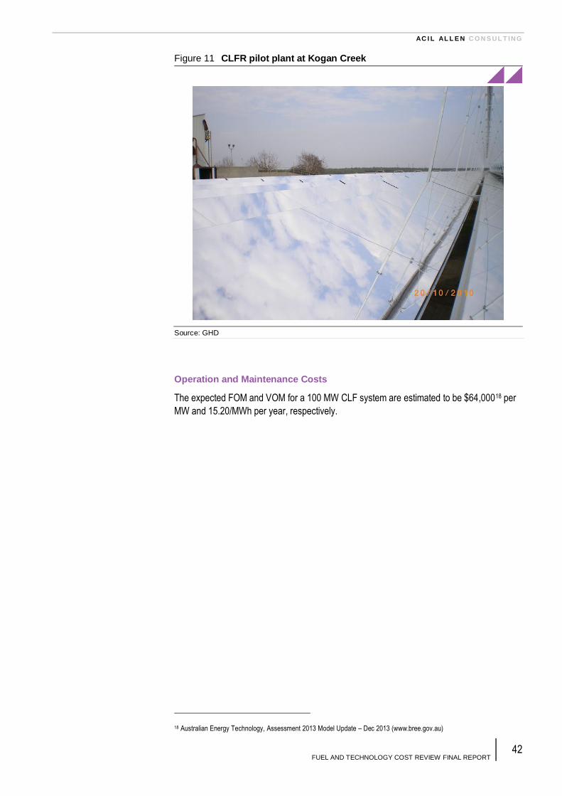
AC I L AL L E N C O N S UL T ING
FUEL AND TECHNOLOGY COST REVIEW FINAL REPORT 42
Figure 11 CLFR pilot plant at Kogan Creek
Source: GHD
Operation and Maintenance Costs
The expected FOM and VOM for a 100 MW CLF system are estimated to be $64,00018 per
MW and 15.20/MWh per year, respectively.
18 Australian Energy Technology, Assessment 2013 Model Update – Dec 2013 (www.bree.gov.au)

AC I L AL L E N C O N S UL T ING
FUEL AND TECHNOLOGY COST REVIEW FINAL REPORT 43
Table 18 Compact Linear Fresnel Technology – Direct Stream Generation –
No Storage
Technology Description Compact Linear Fresnel Technology –
Direct Stream Generation – No Storage
Fuel Type Solar
Capital Costs, A$/kW $4,500
Local Equipment/Construction Costs (includes
commodities)
25%
International Equipment Costs 55%
Labour Costs 20%
Construction Profile % of Capital Cost Year 1 – 50%
Year 2 – 30%
Year 3 – 20%
First Year Assumed Commercially Viable 2016
Typical new entrant size (Generated MW) 100 MW
Economic Life Typical design life is 25 years. There are
no examples of CFLR plants that have gone beyond this period. However, similar
to conventional power plants, their operational life can be extended beyond their design life by regular refurbishing of
the main components or repowering.
Lead time for development (years) 4 years
Minimum stable generation level (% capacity) 10% - output is dependent on solar
resource
Thermal Efficiency (sent out – HHV) N/A
Auxiliary Load (%) 8%
FOM ($/MW/year) for 2014 $64,00019 (without storage)
VOM ($/MWh sent out) 2014 $15.20
Percentage of emissions captured (%) 0%
Emissions rate per kgCO2e/MWh 0
Source: GHD
5.6.2 Central Receiver (with Thermal Storage)
A CSP Central Receiver system, also called power towers, consists of a series of large
mirrors or lenses placed around the tower, called heliostats. Typically, the central receiver
systems have three main components: ground heliostats (mirrors, lenses, or reflectors), a
tower, and a central receiver at the top of the tower. The function of the heliostats is to
capture solar radiation from the sun and re-direct it to a central receiver. A heliostat typically
rotates along two axes, east and west, and north and south, tracking the sun as it moves
throughout the day and the year. Each individual heliostat is guided by a computer
controlled system which follows the sun and optimises total energy output. Electricity is
generated when the concentrated light is converted into heat, which drives a steam turbine
connected to an electrical generator.
The first commercial solar tower system was built by Abengoa Solar of Spain at the Solucar
Platform in the Spanish province of Seville. It began operation in March, 2007 and continues
to this day20.
19 Australian Energy Technology, Assessment 2013 Model Update – Dec 2013 (www.bree.gov.au)
20 Image source: http://solarcellcentral.com/csp_page.html

AC I L AL L E N C O N S UL T ING
FUEL AND TECHNOLOGY COST REVIEW FINAL REPORT 44
Figure 12 Schematics of a CSP tower system
Note: http://mcensustainableenergy.pbworks.com/w/page/32181014/
Source: GHD
Figure 13 CSP tower systems (PS10 & PS20), Seville - Spain (10 & 20MW)
Source: US Department of Energy
Operation and Maintenance Costs
The operating costs of CSP plants are low compared to fossil fuel-fired power plants, but are
still significant. The replacement of receivers and mirrors, due to glass breakage, are a
significant component of the O&M costs. The cost of mirror washing, including water costs,
is significant. Plant insurance and general asset management are also important expenses.
The expected FOM and VOM for a 100 MW CSP tower system are estimated to be
$71,30021 per MW and 5.70/MWh per year, respectively.
21 Australian Energy Technology, Assessment 2013 Model Update – Dec 2013 (www.bree.gov.au)

AC I L AL L E N C O N S UL T ING
FUEL AND TECHNOLOGY COST REVIEW FINAL REPORT 45
Table 19 Central Receiver with 6 hours thermal storage
Technology Description Central Receiver with 6 hours thermal
storage
Fuel Type N/A
Capital Costs, A$/kW $6,700
Local Equipment/Construction Costs (includes
commodities)
20%
International Equipment Costs 55%
Labour Costs 25%
Construction Profile % of Capital Cost Year 1 – 50%
Year 2 – 30%
Year 3 – 20%
First Year Assumed Commercially Viable 2016 – There are currently no central
receiver solar thermal plants under development in Australia.
Typical new entrant size (Generated MW) 100 MW
Economic Life Typical design life is 25 years. There are
no examples of CFLR plants that have gone beyond this period. However, similar to conventional power plants, their
operational life can be extended beyond their design life by regular refurbishing of the main components or repowering.
Lead time for development (years) 4 years
Minimum stable generation level (% capacity) 10% - output is dependent on solar
resource
Thermal Efficiency (sent out – HHV) N/A
Auxiliary Load (%) 10%
FOM ($/MW/year) for 2014 $71,300
VOM ($/MWh sent out) 2014 $5.70
Percentage of emissions captured (%) 0%
Emissions rate per kgCO2e/MWh 0
Source: GHD
5.6.3 Parabolic Trough (with Thermal Storage)
The parabolic trough is a relatively mature power generation technology with extensive
operational history that could be deployed for large-scale installation. This technology was
first commercialised in 1980s. It has improved on costs and efficiency significantly.
Currently, there are several hundreds of MWs in operation in countries such as Spain,
United States, Morocco, Algeria, Egypt, South Africa, India, Mexico and Chile. Parabolic
trough is the most developed technology among all types of solar thermal power plants.
Parabolic trough technology uses a curved, mirrored trough which reflects the direct solar
radiation onto a glass tube containing a fluid (a receiver, absorber or collector) running the
length of the trough and positioned at the focal point of the reflectors. The trough is
parabolic along one axis and linear in the orthogonal axis. Troughs are positioned on a
single axis tracking system to tilt east to west so that the direct radiation remains focused on
the receiver. A heat transfer fluid inside the receiver is used to heat steam in a standard
steam turbine generator arrangement.

AC I L AL L E N C O N S UL T ING
FUEL AND TECHNOLOGY COST REVIEW FINAL REPORT 46
Figure 14 A typical parabolic trough system
Note: Image source: http://www.csp-world.com/resources/technology
Source: GHD
Operation and Maintenance Costs
The operating costs of CSP plants are low compared to fossil fuel-fired power plants, but are
still significant. The replacement of receivers and mirrors, due to glass breakage, are a
significant component of the O&M costs. The cost of mirror washing, including water costs,
is also significant. Plant insurance and general asset management are also important
expenses.
The expected FOM and VOM for a 100 MW CSP parabolic trough system are estimated to
be $72,40022 per MW and 11.40/MWh per year, respectively.
22 Australian Energy Technology, Assessment 2013 Model Update – Dec 2013 (www.bree.gov.au)

AC I L AL L E N C O N S UL T ING
FUEL AND TECHNOLOGY COST REVIEW FINAL REPORT 47
Table 20 Parabolic Trough with 6 hours
Technology Description Parabolic Trough with 6 hours thermal
storage
Fuel Type N/A
Capital Costs, A$/kW sent-out $9,100
Local Equipment/Construction Costs (includes
commodities)
20%
International Equipment Costs 55%
Labour Costs 25%
Construction Profile % of Capital Cost Year 1 – 50%
Year 2 – 30%
Year 3 – 20%
First Year Assumed Commercially Viable 2016
Typical new entrant size (Generated MW) 100 MW
Economic Life 25 years
Lead time for development (years) 4 years
Minimum stable generation level (% capacity) 10% - output is dependent on solar
resource
Thermal Efficiency (sent out – HHV) N/A
Auxiliary Load (%) 10%
FOM ($/MW/year) for 2014 $72,400
VOM ($/MWh sent out) 2014 $11.40
Percentage of emissions captured (%) 0%
Emissions rate per kgCO2e/MWh 0
Source: GHD
5.6.4 Thermal Storage
Parabolic trough and central receiver systems with thermal energy storage typically use a
two-tank, indirect, molten-salt system. The system uses different heat transfer fluids for the
receiver and for storage, and therefore it requires a heat exchanger. Advances in thermal
storage technologies could further improve the uptake of CSP by increasing capacity factors
and enabling systems to take advantage of peak electricity prices. CSP plant capacity
factors extend from 20-28% for plants with no storage to 30 -50% for plants with 6-7.5 hours
of storage23. However, the storage system and additional mirrors increases the installed cost
per kW. For instance, adding a six hour storage option would typically double the CAPEX, or
even higher. The cost of installed generation varies greatly depending on the location,
ownership, the values of key financing terms, available financial incentives, and other
factors.
23 www1.eere.energy.gov - Concentrating Solar Power: Technologies, Cost, and Performance report – May 2010

AC I L AL L E N C O N S UL T ING
FUEL AND TECHNOLOGY COST REVIEW FINAL REPORT 48
Figure 15 Schematics of CSP with thermal storage
Note: Image source: NREL
Source: US Department of Energy
Figure 16 Annual capacity factor for a 100 MW parabolic trough plant as a
function of solar field size and size of thermal energy storage
Note: Data Source: Cost Analysis of Concentrating Solar Power Report – IRENA, June 2012.
Source: GHD
5.6.5 Potential Improvements in CSP Technologies
Currently, the installed costs of CSP systems are high compared to wind or solar PV. For
the purpose of this report, a range of information and studies has been reviewed and
analysed to establish a rule of thumb for cost estimation of CSP systems in Australia based
on system size and thermal storage capacity. Whilst there is a high level of uncertainty with
this, it is apparent that current installed costs per MW are as high as 100% of other
renewable systems.
However, the potential for cost reduction going forward is very high. Reviewing experience
in related industries suggests the most likely result is that cost reduces by around 15% for
every doubling of installed capacity globally. On this basis, and assuming a 20 - 30% per
year projected global growth rate, convergence between cost and value in the Australian
AC I L AL L E N C O N S UL T ING
FUEL AND TECHNOLOGY COST REVIEW FINAL REPORT 49
market is likely to occur not later than 2030 and possibly as soon as 2018, with energy
market price increases due to carbon prices or otherwise also influencing this (ASI24).
The key areas where cost reductions could to be achieved are given by ARENA25 as:
The solar field: mass production and cheaper components, as well as improvements in
design, can help to reduce costs.
The heat transfer fluid: new heat transfer fluids and those capable of higher
temperatures will help to improve storage possibilities and reduce costs. Direct steam
generation is also a possibility, but requires further research.
The storage system: This is closely tied to the heat transfer fluid, as higher
temperatures, notably from solar towers, will reduce the cost of thermal energy storage.
The power block: There is still room for cost reductions, although these will be more
modest than for the other components.
The balance of costs, including project development costs.
5.6.6 Integrated Solar Combined Cycle
Integrated solar combined cycle generation integrates solar thermal technology into
conventional combined cycle gas turbine plant, working effectively to boost the steam cycle
plant to optimise for fuel use and equipment utilisation.
A similar technology is the Kogan Creek Solar Boost project being installed by CS Energy
and AREVA. It involves utilising CLF array to heat steam to CS Energy’s 750 megawatt
coal-fired Kogan Creek Power Station in South West Queensland. The system will augment
the Kogan Creek Power Station’s steam generation and will produce 44 MW of electricity
during peak solar conditions26. This system is similar to an integrated solar combined cycle
in that it supplements the steam cycle to offset fuel consumption (see Figure 17).
The plant considered for this exercise assumes a nominal 500 MW plant including a solar
field sized at a multiple of 1.2 with no thermal storage. The thermal efficiency of this plant is
dependent on the capacity factor achieved due to the available solar resource. Assuming an
average capacity factor of 23% over the year and a thermal efficiency of 50.6% for the base
case CCGT (without integrated solar), the average thermal efficiency would increase to
53.7%. If the solar component were operated at full output, a thermal efficiency of around
64.1% could be achieved.
24 ASI - Realising the potential of Concentrating Solar Power in Australia, May 2012
25 Data Source: Cost Analysis of Concentrating Solar Power Report – ARENA, June 2012
26 Kogan Creek Solar Boost Project, 2014, CS Energy, Available: http://kogansolarboost.com.au/
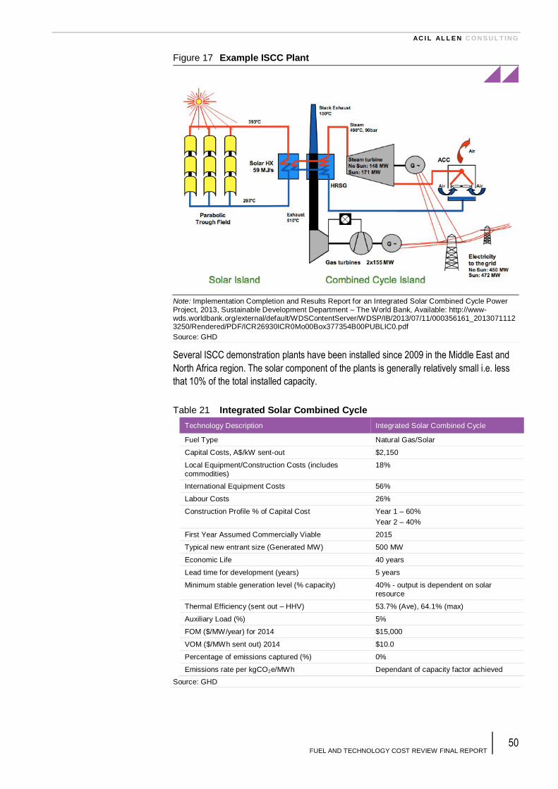
AC I L AL L E N C O N S UL T ING
FUEL AND TECHNOLOGY COST REVIEW FINAL REPORT 50
Figure 17 Example ISCC Plant
Note: Implementation Completion and Results Report for an Integrated Solar Combined Cycle Power Project, 2013, Sustainable Development Department – The World Bank, Available: http://www-wds.worldbank.org/external/default/WDSContentServer/WDSP/IB/2013/07/11/000356161_20130711123250/Rendered/PDF/ICR26930ICR0Mo00Box377354B00PUBLIC0.pdf
Source: GHD
Several ISCC demonstration plants have been installed since 2009 in the Middle East and
North Africa region. The solar component of the plants is generally relatively small i.e. less
that 10% of the total installed capacity.
Table 21 Integrated Solar Combined Cycle
Technology Description Integrated Solar Combined Cycle
Fuel Type Natural Gas/Solar
Capital Costs, A$/kW sent-out $2,150
Local Equipment/Construction Costs (includes
commodities)
18%
International Equipment Costs 56%
Labour Costs 26%
Construction Profile % of Capital Cost Year 1 – 60%
Year 2 – 40%
First Year Assumed Commercially Viable 2015
Typical new entrant size (Generated MW) 500 MW
Economic Life 40 years
Lead time for development (years) 5 years
Minimum stable generation level (% capacity) 40% - output is dependent on solar
resource
Thermal Efficiency (sent out – HHV) 53.7% (Ave), 64.1% (max)
Auxiliary Load (%) 5%
FOM ($/MW/year) for 2014 $15,000
VOM ($/MWh sent out) 2014 $10.0
Percentage of emissions captured (%) 0%
Emissions rate per kgCO2e/MWh Dependant of capacity factor achieved
Source: GHD

AC I L AL L E N C O N S UL T ING
FUEL AND TECHNOLOGY COST REVIEW FINAL REPORT 51
5.7 Wind Technology
Wind power has become one of the mainstream electricity generation sources, and is
considered to be a mature technology among other renewable technologies. It enjoyed the
highest average cumulative growth of 25-30% for 15 consecutive years from late 1990s to
early 2000s. The total installed wind energy capacity worldwide reached 319 GW by the end
of 2013, which contributes close to 4% to the global electricity demand. China installed 16
GW in 2013 and has a total installed capacity of over 91 GW. Asia had the same installed
capacity in 2013 as Europe (119 GW) and is expected to overtake Europe in 2014 as largest
wind continent (WWEA27).
The amount of installed wind power in Australia has doubled in the past five years. The total
installed wind power capacity in Australia by June 2013 was 3,059 MW, 13th position
internationally. China has the first ranking in the world (WWEA).
Wind turbines directly convert the kinetic energy of the wind into electricity. The wind turns
the blades that spin a shaft, which is connected (directly or indirectly via a gearbox) to a
generator that generates electricity. The power generation of wind turbines is determined by
the capacity of the turbine (in kW or MW), the wind resource, height of the turbine and the
diameter of the rotors. Three bladed horizontal axis wind turbines have become the
accepted configuration in most wind power installations. Wind turbine drive train is typically
of two types: direct drive with ring or annular generators (i.e. without a gearbox) and
transmission driven drive train which connects the rotors to a generator. In modern wind
turbines, each blade is pitch-adjusted and controlled by a central computer to extract the
optimum amount of energy from the wind and protect the turbine from extreme wind speeds.
Wind turbines are deigned to operate to wind speeds of up to 90 km/hr; they shut down
automatically until wind speeds return within turbine’s operations range.
Large scale utility wind farms in Australia typically utilise machines in the 2 to 3 MW range
with hub heights of 80 to 100 m above ground level and rotor diameters of 70 to 120 m.
Wind farms are arrays of 50 to 250 turbines. Wind farm sizes in Australia have steadily
grown. 100 MW is considered to be a typical size for the purpose of this report.
5.7.1 Wind Resource
Australia has one of the richest wind resources in the world. Australian wind regime is
dominated by sea breezes and coastal weather systems. For most sites, wind speed is
strongest in mid to later afternoon and weakest at night. Winter months are the windiest time
at most Australian wind sites.
The strength and characteristics of the wind resource have significant impacts on the
delivered cost of electricity generation from a wind turbine. There are a number of factors
such as wind speed distribution characteristics, turbulence intensity, wind shear profile (i.e.
change of wind speed with height) and diurnal / seasonal wind patterns that influence the
strength and quality of the wind resource.
For the purpose of modelling a baseline 100 MW wind farm, an average wind resource that
represents most Australian wind farms and produces a capacity factor of 35% have been
assumed. It is noted that earlier wind farms in Australia have capacity factors of 30% or
lower. However, newer turbines with improved production and higher reliability rates are
expected to support an average 35% capacity factor, or higher.
27 World Wind Energy Association – 2013 Half-Year Report

AC I L AL L E N C O N S UL T ING
FUEL AND TECHNOLOGY COST REVIEW FINAL REPORT 52
5.7.2 Typical New Entrant Size
For the purpose of this report, a typical wind farm size of 100 MW has been considered as
an average new wind farm. The trend for larger wind farm projects has continued in
Australia. Wind farm sizes tend to be limited by a number of factors such as:
Availability of electrical network capacity (i.e. limitation of upgrade and augmentation
costs associated in connecting a larger wind farm)
Wind farm land availability – larger wind farms require large areas of rural land. Signing
in all landowners and satisfying all planning requirements by local regulatory authorities
can constrain wind farm sizes.
Suitable site conditions – favourable wind resource, local topography, site access, ease
of transportation, and wind farm constructability often dictate the size of wind farms.
Off-take agreements – obtaining commercially viable off-take agreements for suitable
long-term periods (i.e. 10 to 15 years).
MacArthur Wind farm with an installed capacity of 420 MW is the largest operational wind
farm in Australia. There are several 500+ MW wind farm projects that are under
consideration in NSW, QLD and WA. It is expected that 100+ MW wind farms will become
more common over the forecast period with an ongoing trend towards deployment of fewer
but larger capacity wind turbines.
5.7.3 Capital Costs Trend
The costs for onshore wind energy experienced significant reductions between 1980 and the
early 2000s with notable increases in turbine performance. However, beginning in about
2003 and continuing through the latter half of the past decade, wind power capital costs
increased, mainly due to rising commodity and raw materials prices, increased labour costs,
improved manufacturer profitability, and turbine up-scaling – thus pushing wind energy’s
costs upward in spite of continued performance improvements. More recently, wind turbine
prices and therefore project capital costs have declined, but still have not returned to the
historical lows observed earlier in the 2000s – however performance improvements have
been maintained. Continued cost reductions are expected through to 2030, but the
anticipated magnitude and pattern of these reductions varies widely and will ultimately be
determined by a variety of technical and non-technical factors.
From mid 2000s, the wind turbine industry has heavily focused in up-scaling of wind
turbines, primarily driven by demands from offshore wind sector. However, efforts to
increase wind turbine reliability did not follow the same pace. Wind turbine suppliers in
recent years have focused their attention to increase wind turbine reliability and lowering
OPEX costs away from up-scaling efforts.
Looking into the future, the cost of wind power is expected to continue to fall, at least on a
global basis and within fixed wind resource classes. Performance improvements associated
with continued turbine up-scaling, use of stronger but lighter structural materials and design
advancements are anticipated that could overall lower capital costs (IEA28). The magnitude
of future cost reductions is nevertheless highly uncertain. It is noted that predictions of the
future cost of onshore wind power that have been done to date have often been the result of
an iterative process that incorporates some combination of historical trends, learning curve
analysis, expert elicitation, and engineering modelling.
28 IEA Wind Task 26 report - The Past and Future Cost of Wind Energy

AC I L AL L E N C O N S UL T ING
FUEL AND TECHNOLOGY COST REVIEW FINAL REPORT 53
A large number of technological and market-based drivers are expected to determine
whether lowering cost projections are ultimately realised. Possible technical drivers include:
More reliable drivetrain technology
Improved manufacturing efficiency
Cost effective O&M strategies
Advancements in power electronics and power conversion
More accurate predictions for energy yield assessments
Advances in new rotor and tower designs by using lighter but stronger materials at lower
costs and more robust high lifting.
Adding to these technical drivers, future environmental and planning policies by local and
federal regulatory authorities such as turbine noise emission guidelines will play an
important role in the cost of installed wind power plants.
5.7.4 Wind farm development and operational life
Wind farms have an operating life of 20 years or longer. However, there are currently no
wind farms in Australia that have been continuously in service for that long. Wind turbines in
Crookwell wind farm in NSW, Denham wind farm in WA, and Thursday Island in QLD are
among the oldest operational machines in Australia.
Development time for a typical wind farm project is in the order of four to seven years from
site identification to commissioning (i.e. commercial operation).
5.7.5 CAPEX Profile Assumptions (FY 2014 to FY 2040)
The following assumptions are made in preparing the CAPEX profile for construction of a
100 MW wind farm project in Australia.
The expected cost in 2014 is taken to be AUD 2,550 per installed kW. This is based on
GHD’s in-house database of recent constructed wind farm projects in Australia.
Wind turbines account for the largest single component of the cost of installed
generation, typically about 72%.
There expected to be reasonable reduction in costs from 2014 to 2020 (11.5%) driven by
increased competition among turbine manufacturers to capture re-emerging Australian
wind market, consolidation of new Asian and mainstream turbine suppliers, increased
economies of scale, and advances in lighter, stronger and more durable core materials
used in turbine rotors, drivetrain, and towers.
It is expected that there would be a period of very limited to nil reduction in costs from
2021-2024. Most grade one wind farm sites (with high wind resource and favourable
planning conditions) have been used up by project developers by then and sites with
lower wind resource in more challenging geographies would be available for
construction. This means that wind turbines with larger rotor diameter compared with
generator size will have to be utilised, and hence the increased levelised cost of energy
will negate the cost reduction factors mentioned above.
From 2025 to 2040, it is expected that costs would continue to drop however the rate
and period of this cost reduction is uncertain.

AC I L AL L E N C O N S UL T ING
FUEL AND TECHNOLOGY COST REVIEW FINAL REPORT 54
The above assumptions are in agreement with ARENA’s29 findings that state “wind turbines
are projected to be 15% cheaper in 2020 than in 2011 and 28% cheaper in 2040”.
Chinese Wind Turbine Suppliers
Among key drivers in lowering the costs for wind power in Australia are expected to be new
entrants into the wind turbine suppliers market such as Chinese OEMs. Chinese and Asian
turbine suppliers such as Goldwind and Suzlon are strongly presented in the Australian
market and have already contributed to lower the capital cost of wind farms. However, since
they are not yet fully recognised by the mainstream lenders and financiers for project
financing, there expected to be another three to five years before they establish themselves
as the dominant players in Australia. With close geographical and trade relationships
between Australia and China, the influence of Chinese wind turbines in contributing to lower
the costs should not be underestimated.
5.7.6 Operation and Maintenance Costs
Operation and maintenance (O&M) costs make up a sizeable share of the total annual costs
of a wind farm. For a new wind farm, O&M costs can easily constitute up to 25% of the total
cost per kWh for over the design life of the wind farm (ARENA, 2012). In recent years, wind
farm O&M costs have been attracting greater attention by project developers and financiers,
as manufacturers attempt to lower these costs significantly by developing new turbine
designs that require fewer regular service visits and less turbine downtime. Wind farm O&M
costs are separated into fixed and variable parts and typically related to:
Planned and unplanned maintenance
Repairs and midlife refurbishments
Insurances
Spare parts, and
Administration and asset management costs.
Cost components such as insurances and planned maintenance (fixed costs) are relatively
easy to estimate. However, costs related to unplanned maintenance and spare parts are
much more difficult to predict. And although all cost components tend to increase as the
turbine gets older, costs for repair and spare parts are particularly influenced by turbine age;
starting low and increasing over time.
Due to dramatic changes in wind turbine technology and turbine sizes during the past two
decades and relative infancy of the wind industry, as well as unavailability of reliable wind
farm operational costs, it is difficult to extrapolate historical O&M costs into future.
Nevertheless, there have been several recent studies that have produced beneficial results.
These investigations indicate that annual average O&M costs have declined substantially
since 1980. In the United States, data for completed projects suggest that total O&M costs
(fixed and variable) have declined from around USD 33/MWh for 24 projects that were
completed in the 1980s to USD 22/MWh for 27 projects installed in the 1990s and to USD
10/MWh for the 65 projects installed in the 2000s (ARENA, 2012).
In Australia, the total O&M costs are generally higher than the US and European costs due
to smaller size of wind industry and unavailability of third party independent O&M service
providers. The expected FOM costs is estimated to be AUD 45,000 per MW annually and
29 RENEWABLE ENERGY TECHNOLOGIES: COST ANALYSIS SERIES, ARENA Volume 1: Power Sector, Issue 5/5 Report
– June 2012.

AC I L AL L E N C O N S UL T ING
FUEL AND TECHNOLOGY COST REVIEW FINAL REPORT 55
VOM is estimated at AUD 13/MWh over the wind farm design life for a 100 MW size wind
farm. It has also been observed that the average length of full-service O&M contracts for
Australian wind farms has increased from 2 years for earlier projects to 5-10 years for
current projects. Average availability guarantees will remain at 96%-97%. The decreasing
cost and increasing contract length suggest that turbine reliability is improving.
Table 22 Wind
Technology Description Wind
Fuel Type N/A
Capital Costs, A$/kW $2,550
Local Equipment/Construction Costs (includes
commodities)
13%
International Equipment Costs 72%
Labour Costs 15%
Construction Profile % of Capital Cost Year 1: 80%
Year 2: 20%
First Year Assumed Commercially Viable 2014
Typical new entrant size 100 MW was assumed for this report.
However, any size can be considered. There are several 500 MW+ wind farms
that are in development stage across Australia
Economic Life Typical design life is 20-25 years. There are no examples of wind farms that have
gone beyond this period in Australia. However, wind farms are anticipated to have an operational life of greater than
their design life by either refurbishing the main components or repowering to newer and larger turbines.
Lead time for development (years) Development time for a typical wind farm
project is 4 to 7 years from site identification to commissioning.
Minimum stable generation level (% capacity) 1% - 3%, depending on turbine type and size
Thermal Efficiency (sent out – HHV) N/A
Thermal Efficiency (sent out – HHV) learning rate (%
improvement per annum)
N/A
Capacity Factor 35%
Auxiliary Load (%) 1%. Auxiliary loads are very low for wind farms and the net capacity factor typically
accounts for them.
FOM ($/MW/year) for 2014 $45,000
VOM ($/MWh sent out) 2014 $13.0
Percentage of emissions captured (%) N/A
Emissions rate per kg CO2e/MWh N/A
Source: GHD
5.8 Wave/Ocean Technology
Wave/ocean energy technologies harness the energy of ocean waves or tidal flows and
convert them into electricity. Wave/ocean technologies are under development for near-
shore, off-shore and far off-shore application. Wave/ocean energy technology is still
considered immature and commercial production of systems at a material scale does not yet
exist. Several prototype technology systems were investigated including point absorbers,
terminator devices, oscillating water columns, attenuators, overtopping devices and surging
devices. The costs are based on a commercial deployment of a wave reaction point
absorber system and does not reflect the current pricing for development scale projects.

AC I L AL L E N C O N S UL T ING
FUEL AND TECHNOLOGY COST REVIEW FINAL REPORT 56
Table 23 Wave/Ocean
Technology Description Wave/Ocean
Fuel Type N/A
Capital Costs, A$/kW sent-out $5,900
Local Equipment/Construction Costs (includes commodities)
30
International Equipment Costs 40
Labour Costs 30
Construction Profile % of Capital Cost Year 1: 60%
Year 2: 40%
First Year Assumed Commercially Viable 2020
Typical new entrant size 20 MW
Economic Life 20 years
Lead time for development (years) 6
Minimum stable generation level (% capacity) 0%
Thermal Efficiency (sent out – HHV) N/A
Auxiliary Load (%) 0.5%
FOM ($/MW/year) for 2014 $40,000
VOM ($/MWh sent out) 2014 $20.0
Percentage of emissions captured (%) N/A
Emissions rate per kg CO2e/MWh N/A
Source: GHD
5.9 Storage Technologies
5.9.1 Large Scale Battery Storage
Battery storage on a large scale is an increasingly attractive solution to complement the
emergence of intermittent renewable energy sources such as solar PV, wind and tidal
energy. Large installations of battery storage can match the total generation to total load
with precision on a second by second basis. Power from batteries can be dispatched almost
instantaneously and effectively produces no emissions once the energy is stored.
Several types of batteries are used for large scale energy storage, all consisting of
electrochemical cells although no one type is suitable for all applications. Technologies
which have been demonstrated at MW-scale and have a growing supply chain include
advanced lead-acid batteries flow batteries and lithium-ion batteries.30
Lead acid batteries are a well-established technology with multiple installations on the grid
for back-up power supply. However they suffer a limited life cycle when regularly cycled over
a substantial rate of change state (ROC), degrading rapidly. Recent advances in materials
and electrolytes have seen increases in cycle life and performance.
Flow batteries have low energy densities although they can be charged and discharged over
almost the entire range of their nameplate capacity.
NREL’s Cost and Performance Data for Power Generation Technologies (Black & Veatch
2012)31 estimates a sodium sulphide installation with an assumed net capacity of 7.2 MW
with 8.1 hours of storage at a cycle efficiency of approximately 75% and gives a capital cost
of US $3,990/kW in 2012 and US $3,890/kW in 2015 dollars. In view of both of these figures
30 Energy Storage, AEMO 100% Renewable Energy Study, 2012, CSIRO, Available:
http://www.climatechange.gov.au/sites/climatechange/files/files/reducing-carbon/APPENDIX8-CSIRO-energy-storage.pdf
31 Cost and Performance Data for Power Generation Technologies, NREL, 2012, Black and Veatch, Available: http://bv.com/docs/reports-studies/nrel-cost-report.pdf
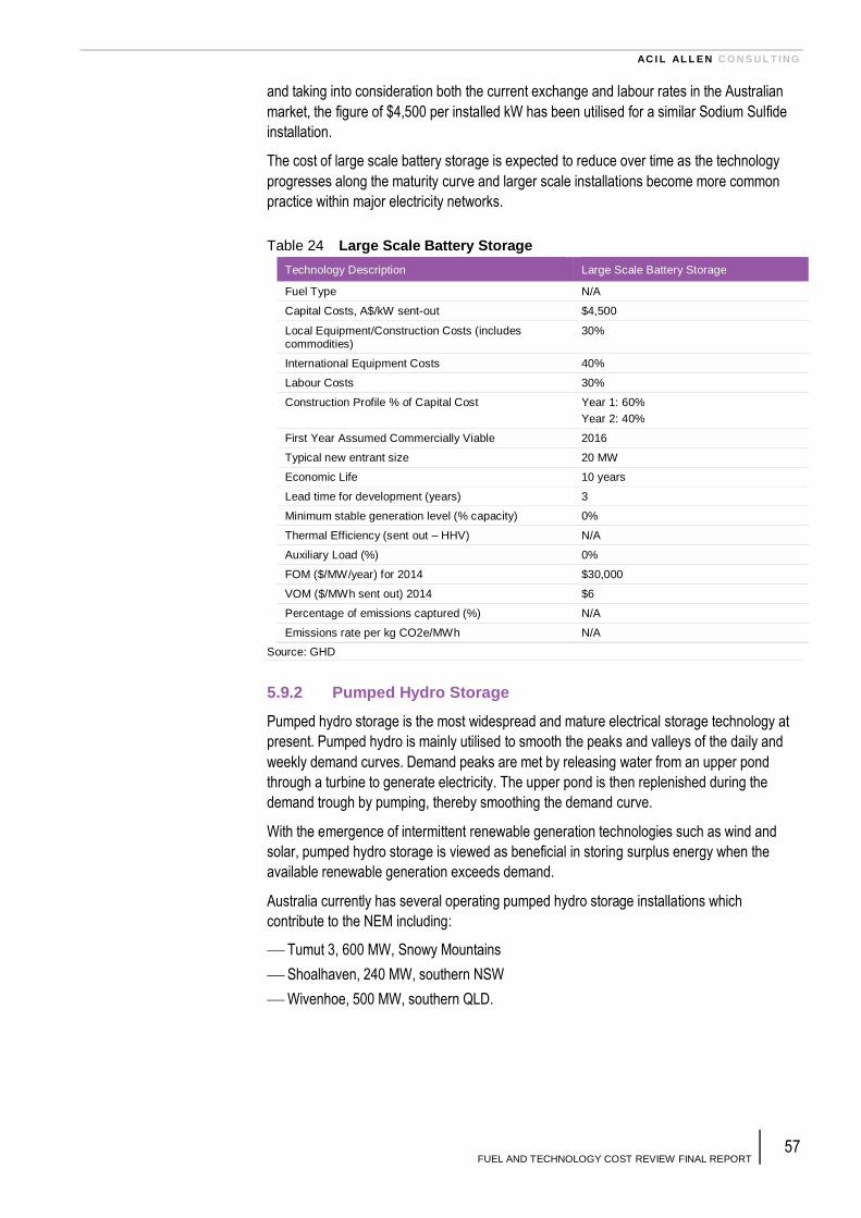
AC I L AL L E N C O N S UL T ING
FUEL AND TECHNOLOGY COST REVIEW FINAL REPORT 57
and taking into consideration both the current exchange and labour rates in the Australian
market, the figure of $4,500 per installed kW has been utilised for a similar Sodium Sulfide
installation.
The cost of large scale battery storage is expected to reduce over time as the technology
progresses along the maturity curve and larger scale installations become more common
practice within major electricity networks.
Table 24 Large Scale Battery Storage
Technology Description Large Scale Battery Storage
Fuel Type N/A
Capital Costs, A$/kW sent-out $4,500
Local Equipment/Construction Costs (includes commodities)
30%
International Equipment Costs 40%
Labour Costs 30%
Construction Profile % of Capital Cost Year 1: 60%
Year 2: 40%
First Year Assumed Commercially Viable 2016
Typical new entrant size 20 MW
Economic Life 10 years
Lead time for development (years) 3
Minimum stable generation level (% capacity) 0%
Thermal Efficiency (sent out – HHV) N/A
Auxiliary Load (%) 0%
FOM ($/MW/year) for 2014 $30,000
VOM ($/MWh sent out) 2014 $6
Percentage of emissions captured (%) N/A
Emissions rate per kg CO2e/MWh N/A
Source: GHD
5.9.2 Pumped Hydro Storage
Pumped hydro storage is the most widespread and mature electrical storage technology at
present. Pumped hydro is mainly utilised to smooth the peaks and valleys of the daily and
weekly demand curves. Demand peaks are met by releasing water from an upper pond
through a turbine to generate electricity. The upper pond is then replenished during the
demand trough by pumping, thereby smoothing the demand curve.
With the emergence of intermittent renewable generation technologies such as wind and
solar, pumped hydro storage is viewed as beneficial in storing surplus energy when the
available renewable generation exceeds demand.
Australia currently has several operating pumped hydro storage installations which
contribute to the NEM including:
Tumut 3, 600 MW, Snowy Mountains
Shoalhaven, 240 MW, southern NSW
Wivenhoe, 500 MW, southern QLD.

AC I L AL L E N C O N S UL T ING
FUEL AND TECHNOLOGY COST REVIEW FINAL REPORT 58
Several additional promising sites were identified in ROAM’s report Pumped Storage
modelling for AEMO 100% Renewables Project, 201232.
This report nominated the following notional cost inputs for estimating installed costs:
Table 25 Pumped Storage Input Costs
Unit costs Cost
Dam wall $ million/m2 0.1
Pipe/tunnel $ million/m 0.5
Mechanical/Electrical $/kW 1000
Source: GHD
Considering these figures and a plant size of 500 MW, the report suggested a benchmark
cost of $3,200/kW.
NREL’s Cost and Performance Data for Power Generation Technologies (Black & Veatch
2012)33 estimates a plant with an assumed net capacity of 500 MW with 10 hours of storage
and gives a capital cost of US $2,230/kW.
In view of both of these figures and taking into consideration both the current exchange and
labour rates in the Australian market, the figure of $3,200 per installed kW has been utilised.
A pumping efficiency (GWh consumed per GWh despatched) of 1.7 has been assumed.
This value, although high, is based on experience with existing plants and is considered
appropriate due to part load operation and varying head in operation.
Pumped hydro storage is considered a mature technology and no cost improvements are
assumed over time.
32 ROAM report on Pumped Storage modelling for AEMO 100% Renewables
project, 2012, ROAM Consulting.
33 Cost and Performance Data for Power Generation Technologies, NREL, 2012, Black and Veatch, Available: http://bv.com/docs/reports-studies/nrel-cost-report.pdf

AC I L AL L E N C O N S UL T ING
FUEL AND TECHNOLOGY COST REVIEW FINAL REPORT 59
Table 26 Pumped Hydro Storage
Technology Description Pumped Hydro Storage
Fuel Type N/A
Capital Costs, A$/kW sent-out $3,200
Local Equipment/Construction Costs (includes commodities)
55%
International Equipment Costs 20%
Labour Costs 25%
Construction Profile % of Capital Cost Year 1: 20
Year 2: 30%
Year 3: 30%
Year 4: 20%
First Year Assumed Commercially Viable 2014
Typical new entrant size 500 MW
Economic Life 50 years
Lead time for development (years) 8 years
Minimum stable generation level (% capacity) 0%
Thermal Efficiency (sent out – HHV) N/A
Auxiliary Load (%) 1%
Pumping Efficiency (GWh pumped per GWh
generated) – within 24 hours
1.7
Pumping Efficiency (GWh pumped per GWh generated) - annual
1.7
FOM ($/MW/year) for 2014 $5000
VOM ($/MWh sent out) 2014 $5.0
Percentage of emissions captured (%) N/A
Emissions rate per kg CO2e/MWh N/A
Source: GHD

AC I L AL L E N C O N S UL T ING
FUEL AND TECHNOLOGY COST REVIEW FINAL REPORT 60
6 Results – Gas prices
6.1 Approach
Long-term price projections for gas have been developed from the outputs of ACIL Allen’s
proprietary gas market model – GMG Australia (GasMark Global Australia). The input
database within GMG Australia is the most comprehensive in Australia and comprises of:
• Over 180 individual gas fields and producing Basins
• 270 individual and aggregated load/demand points, mapped to around 120 market
locations around Australia
• Over 300 pipelines/pipeline segments with actual regulated or estimated commercial
tariff settings.
The geographic representation of the Australian gas network as modelled within this project
is shown in Figure 18. For the purposes of the NTNDP work, the modelling has focused on
Eastern Australia only.
Figure 18 Australian gas network representation
Note: Global demand for Australian LNG is represented by notional offshore receiving terminals and demand points.
Source: GMG Australia

AC I L AL L E N C O N S UL T ING
FUEL AND TECHNOLOGY COST REVIEW FINAL REPORT 61
ACIL Allen has utilised its internal Base Case supply and demand assumptions for this work.
The inputs contain assumptions regarding:
field reserves, production capability and costs
gas demand and the price tolerance and elasticity of this demand
pipeline capacities and tariffs (as well as capability for future augmentations)
LNG plants: capacity, liquefaction tolling and shipping costs.
GMG Australia provides price projections on a nodal basis for each defined node on the
Australian gas grid. Specific nodes are selected to represent each of the 16 NEM zones
within the NTNDP modelling. These are detailed below.
Table 27 NTNDP zone and gas market nodes
NTNDP Zone Gas market node
NQ Townsville
CQ Gladstone
SEQ Swanbank
SWQ Braemar
NNS Wilga Park
NCEN Sydney
SWNSW Wagga
CAN Canberra
NVIC Chiltern
CVIC Ballarat
MEL Melbourne
LV Latrobe
TAS Bell Bay
SESA Ladbroke
ADE Adelaide
NSA Peterborough
Source: ACIL Allen
The availability of gas to support generation in each region is determined by a number of
factors, namely:
The reserves and production capability of various fields (locally and in an aggregate
sense throughout Eastern Australia)
Existing transmission capacity into the zone (if the zone does not have indigenous gas
resources)
The potential for new or additional transmission capacity.
Prices from GMG Australia can be interpreted as annual market clearing prices – similar to
those that would apply within liquid spot markets. The NEM now has access to several spot
gas markets: the Victorian spot market, the Short-term Trading Markets (STTMs) at Sydney,
Adelaide and Brisbane and the recently opened Wallumbilla Gas Supply Hub. Whilst trading
in these markets currently only comprises a very small proportion of gas supply, it is likely
that these will develop over time and become pricing markers for domestic gas contracts.
Legacy gas contracts
Given the large divergence between prices within legacy gas supply contracts and current
contract prices, we have chosen to use current price markers as being the representative
cost for existing generators. Most generators no longer consider prices under existing
contracts to be their marginal cost of fuel, but rather look to the opportunity cost of the

AC I L AL L E N C O N S UL T ING
FUEL AND TECHNOLOGY COST REVIEW FINAL REPORT 62
commodity. This is illustrated by the recent decision by Stanwell to sell contracted gas to
other users rather than utilise it at Swanbank E. If the gas has a higher value elsewhere and
on-sale is feasible, then this should represent the marginal fuel cost. It is likely that a
number of baseload/intermediate gas plant will switch to peaking roles over the next few
years as anticipated wholesale gas price rises materialise.
For this reason, ACIL Allen has projected gas prices for each network node and used these
values for all generators within that NTNDP zone, irrespective of existing gas supply
contractual positions. A mark-up of $2/GJ (Real 2014-15 dollars) has been applied to
peaking generators reflecting the fact that spot gas prices during periods when peakers are
seeking to run will generally be higher than average annual values.
NTNDP scenarios
Within GMG Australia gas prices are set based on domestic gas-on-gas competition
between producers, taking into account acreage and contracts for supply to export markets.
Adjustments between the NTNDP scenarios have been made for gas production costs and
the degree to which prospective and contingent gas resources ultimately are firmed up into
proven and probable gas reserves. The assumption changes between scenarios is
summarised below.
Table 28 NTNDP scenario assumptions
NTNDP scenario Treatment within gas market modelling
High energy consumption from a centralised
source
Lower production costs for unconventional gas (lower drilling and completion costs,
higher well productivity and ultimate recovery); 8 LNG trains developed in QLD in the period to 2027
Medium energy consumption from a
centralised source
ACIL Allen base case demand and supply assumptions; 6 LNG trains currently
committed, no new LNG developments (committed 6 LNG trains only)
Low energy consumption from a centralised source
Increased production costs for unconventional gas (higher drilling and completion
costs, lower well productivity and ultimate recovery); lower ultimate resource conversion to reserves; committed 6 LNG trains only
Source: ACIL Allen
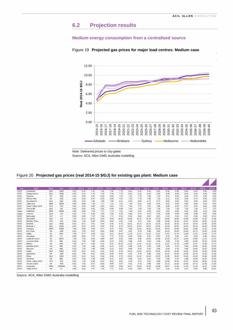
AC I L AL L E N C O N S UL T ING
FUEL AND TECHNOLOGY COST REVIEW FINAL REPORT 63
6.2 Projection results
Medium energy consumption from a centralised source
Figure 19 Projected gas prices for major load centres: Medium case
Note: Delivered prices to city-gates
Source: ACIL Allen GMG Australia modelling
Figure 20 Projected gas prices (real 2014-15 $/GJ) for existing gas plant: Medium case
Source: ACIL Allen GMG Australia modelling
0.00
2.00
4.00
6.00
8.00
10.00
12.00
201
4-1
5
201
5-1
6
201
6-1
7
201
7-1
8
201
8-1
9
201
9-2
0
202
0-2
1
202
1-2
2
202
2-2
3
202
3-2
4
202
4-2
5
202
5-2
6
202
6-2
7
202
7-2
8
202
8-2
9
202
9-3
0
203
0-3
1
203
1-3
2
203
2-3
3
203
3-3
4
203
4-3
5
203
5-3
6
203
6-3
7
203
7-3
8
203
8-3
9
203
9-4
0
Real
2014-1
5 $
/GJ
Adelaide Brisbane Sydney Melbourne Wallumbilla
Ty pe Station Region Zone 2014-15 2015-16 2016-17 2017-18 2018-19 2019-20 2020-21 2021-22 2022-23 2023-24 2024-25 2025-26 2026-27 2027-28 2028-29 2029-30
CCGT Condamine QLD SWQ 4.52 6.14 7.41 7.34 7.34 7.73 8.01 8.15 8.24 8.25 8.35 8.45 8.44 8.43 8.46 8.50
CCGT Darling Dow ns QLD SWQ 4.52 6.14 7.41 7.34 7.34 7.73 8.01 8.15 8.24 8.25 8.35 8.45 8.44 8.43 8.46 8.50
CCGT Osborne SA ADE 4.91 5.63 6.47 6.63 6.69 7.07 7.51 7.79 7.86 7.92 8.12 8.30 8.49 8.73 9.00 9.20
CCGT Pelican Point SA ADE 4.91 5.63 6.47 6.63 6.69 7.07 7.51 7.79 7.86 7.92 8.12 8.30 8.49 8.73 9.00 9.20
CCGT Sw anbank E QLD SEQ 4.80 6.63 7.96 7.89 7.89 8.21 8.56 8.69 8.72 8.72 8.82 8.92 8.91 8.90 8.93 8.97
CCGT Tallaw arra NSW NCEN 5.84 6.89 7.34 7.17 7.13 7.51 7.94 8.22 8.29 8.34 8.52 8.69 8.81 8.96 9.23 9.43
CCGT Tamar Valley CCGT TAS TAS 4.81 5.54 6.38 6.54 6.62 7.01 7.45 7.74 7.81 7.88 8.06 8.25 8.37 8.53 8.81 9.02
CCGT Tow nsville QLD NQ 5.92 5.92 5.91 6.25 6.58 6.94 7.30 7.30 7.30 7.29 7.29 7.28 7.28 7.28 7.27 7.27
Cogen Smithfield NSW NCEN 5.84 6.89 7.34 7.17 7.13 7.51 7.94 8.22 8.29 8.34 8.52 8.69 8.81 8.96 9.23 9.43
Cogen Yarw un QLD CQ 5.23 7.14 8.20 7.92 7.93 8.25 8.60 8.74 8.78 8.78 8.89 8.99 8.99 8.98 9.02 9.06
OCGT Bairnsdale VIC LV 5.90 6.63 7.47 7.64 7.71 8.10 8.54 8.83 8.91 8.97 9.15 9.34 9.47 9.63 9.90 10.11
OCGT Barcaldine QLD CQ 7.23 9.14 10.20 9.92 9.93 10.25 10.60 10.74 10.78 10.78 10.89 10.99 10.99 10.98 11.02 11.06
OCGT Bell Bay Three TAS TAS 6.81 7.54 8.38 8.54 8.62 9.01 9.45 9.74 9.81 9.88 10.06 10.25 10.37 10.53 10.81 11.02
OCGT Braemar QLD SWQ 6.52 8.14 9.41 9.34 9.34 9.73 10.01 10.15 10.24 10.25 10.35 10.45 10.44 10.43 10.46 10.50
OCGT Braemar 2 QLD SWQ 6.52 8.14 9.41 9.34 9.34 9.73 10.01 10.15 10.24 10.25 10.35 10.45 10.44 10.43 10.46 10.50
OCGT Colongra NSW NCEN 7.84 8.89 9.34 9.17 9.13 9.51 9.94 10.22 10.29 10.34 10.52 10.69 10.81 10.96 11.23 11.43
OCGT Dry Creek SA ADE 6.91 7.63 8.47 8.63 8.69 9.07 9.51 9.79 9.86 9.92 10.12 10.30 10.49 10.73 11.00 11.20
OCGT Hallett SA NSA 7.50 8.77 9.39 9.31 9.31 10.18 11.20 11.47 11.52 11.51 11.61 11.70 11.69 11.67 11.69 11.72
OCGT Jeeralang VIC LV 5.90 6.63 7.47 7.64 7.71 8.10 8.54 8.83 8.91 8.97 9.15 9.34 9.47 9.63 9.90 10.11
OCGT Ladbroke Grove SA SESA 7.09 7.81 8.64 8.80 8.87 9.25 9.68 9.96 10.03 10.09 10.29 10.47 10.65 10.89 11.16 11.37
OCGT Laverton North VIC MEL 6.32 7.05 7.89 8.06 8.13 8.52 8.96 9.25 9.33 9.39 9.58 9.76 9.89 10.05 10.32 10.53
OCGT Mintaro SA NSA 7.50 8.77 9.39 9.31 9.31 10.18 11.20 11.47 11.52 11.51 11.61 11.70 11.69 11.67 11.69 11.72
OCGT Mortlake OCGT VIC MEL 6.32 7.05 7.89 8.06 8.13 8.52 8.96 9.25 9.33 9.39 9.58 9.76 9.89 10.05 10.32 10.53
OCGT New port VIC MEL 6.32 7.05 7.89 8.06 8.13 8.52 8.96 9.25 9.33 9.39 9.58 9.76 9.89 10.05 10.32 10.53
OCGT Oakey QLD SWQ 6.52 8.14 9.41 9.34 9.34 9.73 10.01 10.15 10.24 10.25 10.35 10.45 10.44 10.43 10.46 10.50
OCGT Quarantine SA ADE 6.91 7.63 8.47 8.63 8.69 9.07 9.51 9.79 9.86 9.92 10.12 10.30 10.49 10.73 11.00 11.20
OCGT Roma QLD SWQ 6.52 8.14 9.41 9.34 9.34 9.73 10.01 10.15 10.24 10.25 10.35 10.45 10.44 10.43 10.46 10.50
OCGT Somerton VIC MEL 6.32 7.05 7.89 8.06 8.13 8.52 8.96 9.25 9.33 9.39 9.58 9.76 9.89 10.05 10.32 10.53
OCGT Tamar Valley OCGT TAS TAS 6.81 7.54 8.38 8.54 8.62 9.01 9.45 9.74 9.81 9.88 10.06 10.25 10.37 10.53 10.81 11.02
OCGT Torrens Island SA ADE 6.91 7.63 8.47 8.63 8.69 9.07 9.51 9.79 9.86 9.92 10.12 10.30 10.49 10.73 11.00 11.20
OCGT Uranquinty NSW SWNSW 7.62 8.38 9.22 9.38 9.45 9.83 10.27 10.56 10.63 10.69 10.87 11.06 11.18 11.33 11.61 11.81
OCGT Valley Pow er VIC LV 5.90 6.63 7.47 7.64 7.71 8.10 8.54 8.83 8.91 8.97 9.15 9.34 9.47 9.63 9.90 10.11

AC I L AL L E N C O N S UL T ING
FUEL AND TECHNOLOGY COST REVIEW FINAL REPORT 64
Figure 21 Projected gas prices (real 2014-15 $/GJ) for new entrants: Medium case
Source: ACIL Allen GMG Australia modelling
High energy consumption from a centralised source
Figure 22 Projected gas prices for major load centres: High case
Note: Delivered prices to city-gates
Source: ACIL Allen GMG Australia modelling
Technology Zone 2014-15 2015-16 2016-17 2017-18 2018-19 2019-20 2020-21 2021-22 2022-23 2023-24 2024-25 2025-26 2026-27 2027-28 2028-29 2029-30
CCGT - Without CCS (ADE) ADE 4.91 5.63 6.47 6.63 6.69 7.07 7.51 7.79 7.86 7.92 8.12 8.30 8.49 8.73 9.00 9.20
CCGT - Without CCS (CAN) CAN 5.45 6.50 6.95 6.79 6.75 7.13 7.56 7.85 7.92 7.97 8.15 8.33 8.45 8.60 8.87 9.07
CCGT - Without CCS (CQ) CQ 5.23 7.14 8.20 7.92 7.93 8.25 8.60 8.74 8.78 8.78 8.89 8.99 8.99 8.98 9.02 9.06
CCGT - Without CCS (CVIC) CVIC 4.51 5.24 6.08 6.24 6.31 6.70 7.14 7.43 7.50 7.57 7.77 7.96 8.15 8.39 8.66 8.87
CCGT - Without CCS (LV) LV 3.90 4.63 5.47 5.64 5.71 6.10 6.54 6.83 6.91 6.97 7.15 7.34 7.47 7.63 7.90 8.11
CCGT - Without CCS (MEL) MEL 4.32 5.05 5.89 6.06 6.13 6.52 6.96 7.25 7.33 7.39 7.58 7.76 7.89 8.05 8.32 8.53
CCGT - Without CCS (NCEN) NCEN 5.84 6.89 7.34 7.17 7.13 7.51 7.94 8.22 8.29 8.34 8.52 8.69 8.81 8.96 9.23 9.43
CCGT - Without CCS (NNS) NNS 4.51 4.71 5.98 7.02 6.98 7.29 7.54 7.68 7.71 7.71 7.84 8.02 8.14 8.29 8.55 8.76
CCGT - Without CCS (NQ) NQ 5.92 5.92 5.91 6.25 6.58 6.94 7.30 7.30 7.30 7.29 7.29 7.28 7.28 7.28 7.27 7.27
CCGT - Without CCS (NSA) NSA 5.50 6.77 7.39 7.31 7.31 8.18 9.20 9.47 9.52 9.51 9.61 9.70 9.69 9.67 9.69 9.72
CCGT - Without CCS (NVIC) NVIC 4.92 5.65 6.49 6.66 6.73 7.12 7.56 7.85 7.93 7.99 8.18 8.36 8.49 8.65 8.92 9.13
CCGT - Without CCS (SEQ) SEQ 4.80 6.63 7.96 7.89 7.89 8.21 8.56 8.69 8.72 8.72 8.82 8.92 8.91 8.90 8.93 8.97
CCGT - Without CCS (SESA) SESA 5.09 5.81 6.64 6.80 6.87 7.25 7.68 7.96 8.03 8.09 8.29 8.47 8.65 8.89 9.16 9.37
CCGT - Without CCS (SWNSW) SWNSW 5.62 6.38 7.22 7.38 7.45 7.83 8.27 8.56 8.63 8.69 8.87 9.06 9.18 9.33 9.61 9.81
CCGT - Without CCS (SWQ) SWQ 4.52 6.14 7.41 7.34 7.34 7.73 8.01 8.15 8.24 8.25 8.35 8.45 8.44 8.43 8.46 8.50
CCGT - Without CCS (TAS) TAS 4.81 5.54 6.38 6.54 6.62 7.01 7.45 7.74 7.81 7.88 8.06 8.25 8.37 8.53 8.81 9.02
OCGT - Without CCS (ADE) ADE 6.91 7.63 8.47 8.63 8.69 9.07 9.51 9.79 9.86 9.92 10.12 10.30 10.49 10.73 11.00 11.20
OCGT - Without CCS (CAN) CAN 7.45 8.50 8.95 8.79 8.75 9.13 9.56 9.85 9.92 9.97 10.15 10.33 10.45 10.60 10.87 11.07
OCGT - Without CCS (CQ) CQ 7.23 9.14 10.20 9.92 9.93 10.25 10.60 10.74 10.78 10.78 10.89 10.99 10.99 10.98 11.02 11.06
OCGT - Without CCS (CVIC) CVIC 6.51 7.24 8.08 8.24 8.31 8.70 9.14 9.43 9.50 9.57 9.77 9.96 10.15 10.39 10.66 10.87
OCGT - Without CCS (LV) LV 5.90 6.63 7.47 7.64 7.71 8.10 8.54 8.83 8.91 8.97 9.15 9.34 9.47 9.63 9.90 10.11
OCGT - Without CCS (MEL) MEL 6.32 7.05 7.89 8.06 8.13 8.52 8.96 9.25 9.33 9.39 9.58 9.76 9.89 10.05 10.32 10.53
OCGT - Without CCS (NCEN) NCEN 7.84 8.89 9.34 9.17 9.13 9.51 9.94 10.22 10.29 10.34 10.52 10.69 10.81 10.96 11.23 11.43
OCGT - Without CCS (NNS) NNS 6.51 6.71 7.98 9.02 8.98 9.29 9.54 9.68 9.71 9.71 9.84 10.02 10.14 10.29 10.55 10.76
OCGT - Without CCS (NQ) NQ 7.92 7.92 7.91 8.25 8.58 8.94 9.30 9.30 9.30 9.29 9.29 9.28 9.28 9.28 9.27 9.27
OCGT - Without CCS (NSA) NSA 7.50 8.77 9.39 9.31 9.31 10.18 11.20 11.47 11.52 11.51 11.61 11.70 11.69 11.67 11.69 11.72
OCGT - Without CCS (NVIC) NVIC 6.92 7.65 8.49 8.66 8.73 9.12 9.56 9.85 9.93 9.99 10.18 10.36 10.49 10.65 10.92 11.13
OCGT - Without CCS (SEQ) SEQ 6.80 8.63 9.96 9.89 9.89 10.21 10.56 10.69 10.72 10.72 10.82 10.92 10.91 10.90 10.93 10.97
OCGT - Without CCS (SESA) SESA 7.09 7.81 8.64 8.80 8.87 9.25 9.68 9.96 10.03 10.09 10.29 10.47 10.65 10.89 11.16 11.37
OCGT - Without CCS (SWNSW) SWNSW 7.62 8.38 9.22 9.38 9.45 9.83 10.27 10.56 10.63 10.69 10.87 11.06 11.18 11.33 11.61 11.81
OCGT - Without CCS (SWQ) SWQ 6.52 8.14 9.41 9.34 9.34 9.73 10.01 10.15 10.24 10.25 10.35 10.45 10.44 10.43 10.46 10.50
OCGT - Without CCS (TAS) TAS 6.81 7.54 8.38 8.54 8.62 9.01 9.45 9.74 9.81 9.88 10.06 10.25 10.37 10.53 10.81 11.02
0.00
1.00
2.00
3.00
4.00
5.00
6.00
7.00
8.00
9.00
10.00
201
4-1
5
201
5-1
6
201
6-1
7
201
7-1
8
201
8-1
9
201
9-2
0
202
0-2
1
202
1-2
2
202
2-2
3
202
3-2
4
202
4-2
5
202
5-2
6
202
6-2
7
202
7-2
8
202
8-2
9
202
9-3
0
203
0-3
1
203
1-3
2
203
2-3
3
203
3-3
4
203
4-3
5
203
5-3
6
203
6-3
7
203
7-3
8
203
8-3
9
203
9-4
0
Real
2014-1
5 $
/GJ
Adelaide Brisbane Sydney Melbourne Wallumbilla

AC I L AL L E N C O N S UL T ING
FUEL AND TECHNOLOGY COST REVIEW FINAL REPORT 65
Figure 23 Projected gas prices (real 2014-15 $/GJ) for existing gas plant: High case
Source: ACIL Allen GMG Australia modelling
Figure 24 Projected gas prices (real 2014-15 $/GJ) for new entrants: High case
Source: ACIL Allen GMG Australia modelling
Ty pe Station Region Zone 2014-15 2015-16 2016-17 2017-18 2018-19 2019-20 2020-21 2021-22 2022-23 2023-24 2024-25 2025-26 2026-27 2027-28 2028-29 2029-30
CCGT Condamine QLD SWQ 3.58 5.25 6.71 6.27 5.89 6.08 6.45 6.71 6.60 6.47 6.47 6.56 6.87 7.12 7.14 7.15
CCGT Darling Dow ns QLD SWQ 3.58 5.25 6.71 6.27 5.89 6.08 6.45 6.71 6.60 6.47 6.47 6.56 6.87 7.12 7.14 7.15
CCGT Osborne SA ADE 4.52 5.35 6.19 5.99 5.99 6.45 7.00 7.27 7.27 7.26 7.40 7.62 7.75 7.80 7.81 7.83
CCGT Pelican Point SA ADE 4.52 5.35 6.19 5.99 5.99 6.45 7.00 7.27 7.27 7.26 7.40 7.62 7.75 7.80 7.81 7.83
CCGT Sw anbank E QLD SEQ 3.87 5.74 7.33 6.89 6.44 6.56 6.99 7.26 7.07 6.95 6.95 7.03 7.34 7.59 7.61 7.62
CCGT Tallaw arra NSW NCEN 5.16 6.05 6.76 6.50 6.42 6.89 7.43 7.70 7.69 7.68 7.81 8.04 8.17 8.21 8.22 8.24
CCGT Tamar Valley CCGT TAS TAS 4.41 5.26 6.10 5.91 5.91 6.38 6.93 7.22 7.22 7.22 7.36 7.59 7.73 7.78 7.80 7.83
CCGT Tow nsville QLD NQ 4.91 4.91 4.90 4.90 4.90 4.89 4.89 4.88 4.88 4.99 5.10 5.43 6.33 6.90 6.92 6.92
Cogen Smithfield NSW NCEN 5.16 6.05 6.76 6.50 6.42 6.89 7.43 7.70 7.69 7.68 7.81 8.04 8.17 8.21 8.22 8.24
Cogen Yarw un QLD CQ 4.29 6.25 7.56 6.92 6.48 6.60 7.04 7.31 7.13 7.01 7.02 7.10 7.27 7.37 7.40 7.41
OCGT Bairnsdale VIC LV 5.51 6.35 7.20 7.00 7.01 7.48 8.03 8.31 8.31 8.31 8.45 8.69 8.82 8.87 8.90 8.92
OCGT Barcaldine QLD CQ 6.29 8.25 9.56 8.92 8.48 8.60 9.04 9.31 9.13 9.01 9.02 9.10 9.27 9.37 9.40 9.41
OCGT Bell Bay Three TAS TAS 6.41 7.26 8.10 7.91 7.91 8.38 8.93 9.22 9.22 9.22 9.36 9.59 9.73 9.78 9.80 9.83
OCGT Braemar QLD SWQ 5.58 7.25 8.71 8.27 7.89 8.08 8.45 8.71 8.60 8.47 8.47 8.56 8.87 9.12 9.14 9.15
OCGT Braemar 2 QLD SWQ 5.58 7.25 8.71 8.27 7.89 8.08 8.45 8.71 8.60 8.47 8.47 8.56 8.87 9.12 9.14 9.15
OCGT Colongra NSW NCEN 7.16 8.05 8.76 8.50 8.42 8.89 9.43 9.70 9.69 9.68 9.81 10.04 10.17 10.21 10.22 10.24
OCGT Dry Creek SA ADE 6.52 7.35 8.19 7.99 7.99 8.45 9.00 9.27 9.27 9.26 9.40 9.62 9.75 9.80 9.81 9.83
OCGT Hallett SA NSA 6.81 7.88 8.75 8.31 8.05 8.68 9.62 10.06 9.87 9.74 9.73 9.81 9.97 10.06 10.07 10.08
OCGT Jeeralang VIC LV 5.51 6.35 7.20 7.00 7.01 7.48 8.03 8.31 8.31 8.31 8.45 8.69 8.82 8.87 8.90 8.92
OCGT Ladbroke Grove SA SESA 6.69 7.53 8.37 8.17 8.16 8.63 9.17 9.44 9.44 9.43 9.57 9.79 9.92 9.96 9.98 10.00
OCGT Laverton North VIC MEL 5.93 6.77 7.62 7.43 7.43 7.90 8.45 8.73 8.73 8.73 8.88 9.11 9.24 9.29 9.32 9.34
OCGT Mintaro SA NSA 6.81 7.88 8.75 8.31 8.05 8.68 9.62 10.06 9.87 9.74 9.73 9.81 9.97 10.06 10.07 10.08
OCGT Mortlake OCGT VIC MEL 5.93 6.77 7.62 7.43 7.43 7.90 8.45 8.73 8.73 8.73 8.88 9.11 9.24 9.29 9.32 9.34
OCGT New port VIC MEL 5.93 6.77 7.62 7.43 7.43 7.90 8.45 8.73 8.73 8.73 8.88 9.11 9.24 9.29 9.32 9.34
OCGT Oakey QLD SWQ 5.58 7.25 8.71 8.27 7.89 8.08 8.45 8.71 8.60 8.47 8.47 8.56 8.87 9.12 9.14 9.15
OCGT Quarantine SA ADE 6.52 7.35 8.19 7.99 7.99 8.45 9.00 9.27 9.27 9.26 9.40 9.62 9.75 9.80 9.81 9.83
OCGT Roma QLD SWQ 5.58 7.25 8.71 8.27 7.89 8.08 8.45 8.71 8.60 8.47 8.47 8.56 8.87 9.12 9.14 9.15
OCGT Somerton VIC MEL 5.93 6.77 7.62 7.43 7.43 7.90 8.45 8.73 8.73 8.73 8.88 9.11 9.24 9.29 9.32 9.34
OCGT Tamar Valley OCGT TAS TAS 6.41 7.26 8.10 7.91 7.91 8.38 8.93 9.22 9.22 9.22 9.36 9.59 9.73 9.78 9.80 9.83
OCGT Torrens Island SA ADE 6.52 7.35 8.19 7.99 7.99 8.45 9.00 9.27 9.27 9.26 9.40 9.62 9.75 9.80 9.81 9.83
OCGT Uranquinty NSW SWNSW 7.23 8.10 8.94 8.70 8.65 9.16 9.76 10.04 10.03 10.03 10.17 10.39 10.52 10.58 10.60 10.62
OCGT Valley Pow er VIC LV 5.51 6.35 7.20 7.00 7.01 7.48 8.03 8.31 8.31 8.31 8.45 8.69 8.82 8.87 8.90 8.92
Technology Zone 2014-15 2015-16 2016-17 2017-18 2018-19 2019-20 2020-21 2021-22 2022-23 2023-24 2024-25 2025-26 2026-27 2027-28 2028-29 2029-30
CCGT - Without CCS (ADE) ADE 4.52 5.35 6.19 5.99 5.99 6.45 7.00 7.27 7.27 7.26 7.40 7.62 7.75 7.80 7.81 7.83
CCGT - Without CCS (CAN) CAN 4.77 5.67 6.37 6.11 6.04 6.51 7.05 7.33 7.32 7.31 7.45 7.67 7.80 7.85 7.86 7.88
CCGT - Without CCS (CQ) CQ 4.29 6.25 7.56 6.92 6.48 6.60 7.04 7.31 7.13 7.01 7.02 7.10 7.27 7.37 7.40 7.41
CCGT - Without CCS (CVIC) CVIC 4.12 4.96 5.80 5.61 5.61 6.08 6.63 6.91 6.91 6.90 7.05 7.28 7.41 7.46 7.48 7.51
CCGT - Without CCS (LV) LV 3.51 4.35 5.20 5.00 5.01 5.48 6.03 6.31 6.31 6.31 6.45 6.69 6.82 6.87 6.90 6.92
CCGT - Without CCS (MEL) MEL 3.93 4.77 5.62 5.43 5.43 5.90 6.45 6.73 6.73 6.73 6.88 7.11 7.24 7.29 7.32 7.34
CCGT - Without CCS (NCEN) NCEN 5.16 6.05 6.76 6.50 6.42 6.89 7.43 7.70 7.69 7.68 7.81 8.04 8.17 8.21 8.22 8.24
CCGT - Without CCS (NNS) NNS 3.68 3.77 5.19 6.35 6.27 6.74 7.02 7.03 7.02 7.01 7.14 7.37 7.49 7.53 7.55 7.57
CCGT - Without CCS (NQ) NQ 4.91 4.91 4.90 4.90 4.90 4.89 4.89 4.88 4.88 4.99 5.10 5.43 6.33 6.90 6.92 6.92
CCGT - Without CCS (NSA) NSA 4.81 5.88 6.75 6.31 6.05 6.68 7.62 8.06 7.87 7.74 7.73 7.81 7.97 8.06 8.07 8.08
CCGT - Without CCS (NVIC) NVIC 4.53 5.37 6.22 6.03 6.03 6.50 7.05 7.33 7.33 7.33 7.47 7.71 7.84 7.89 7.92 7.94
CCGT - Without CCS (SEQ) SEQ 3.87 5.74 7.33 6.89 6.44 6.56 6.99 7.26 7.07 6.95 6.95 7.03 7.34 7.59 7.61 7.62
CCGT - Without CCS (SESA) SESA 4.69 5.53 6.37 6.17 6.16 6.63 7.17 7.44 7.44 7.43 7.57 7.79 7.92 7.96 7.98 8.00
CCGT - Without CCS (SWNSW) SWNSW 5.23 6.10 6.94 6.70 6.65 7.16 7.76 8.04 8.03 8.03 8.17 8.39 8.52 8.58 8.60 8.62
CCGT - Without CCS (SWQ) SWQ 3.58 5.25 6.71 6.27 5.89 6.08 6.45 6.71 6.60 6.47 6.47 6.56 6.87 7.12 7.14 7.15
CCGT - Without CCS (TAS) TAS 4.41 5.26 6.10 5.91 5.91 6.38 6.93 7.22 7.22 7.22 7.36 7.59 7.73 7.78 7.80 7.83
OCGT - Without CCS (ADE) ADE 6.52 7.35 8.19 7.99 7.99 8.45 9.00 9.27 9.27 9.26 9.40 9.62 9.75 9.80 9.81 9.83
OCGT - Without CCS (CAN) CAN 6.77 7.67 8.37 8.11 8.04 8.51 9.05 9.33 9.32 9.31 9.45 9.67 9.80 9.85 9.86 9.88
OCGT - Without CCS (CQ) CQ 6.29 8.25 9.56 8.92 8.48 8.60 9.04 9.31 9.13 9.01 9.02 9.10 9.27 9.37 9.40 9.41
OCGT - Without CCS (CVIC) CVIC 6.12 6.96 7.80 7.61 7.61 8.08 8.63 8.91 8.91 8.90 9.05 9.28 9.41 9.46 9.48 9.51
OCGT - Without CCS (LV) LV 5.51 6.35 7.20 7.00 7.01 7.48 8.03 8.31 8.31 8.31 8.45 8.69 8.82 8.87 8.90 8.92
OCGT - Without CCS (MEL) MEL 5.93 6.77 7.62 7.43 7.43 7.90 8.45 8.73 8.73 8.73 8.88 9.11 9.24 9.29 9.32 9.34
OCGT - Without CCS (NCEN) NCEN 7.16 8.05 8.76 8.50 8.42 8.89 9.43 9.70 9.69 9.68 9.81 10.04 10.17 10.21 10.22 10.24
OCGT - Without CCS (NNS) NNS 5.68 5.77 7.19 8.35 8.27 8.74 9.02 9.03 9.02 9.01 9.14 9.37 9.49 9.53 9.55 9.57
OCGT - Without CCS (NQ) NQ 6.91 6.91 6.90 6.90 6.90 6.89 6.89 6.88 6.88 6.99 7.10 7.43 8.33 8.90 8.92 8.92
OCGT - Without CCS (NSA) NSA 6.81 7.88 8.75 8.31 8.05 8.68 9.62 10.06 9.87 9.74 9.73 9.81 9.97 10.06 10.07 10.08
OCGT - Without CCS (NVIC) NVIC 6.53 7.37 8.22 8.03 8.03 8.50 9.05 9.33 9.33 9.33 9.47 9.71 9.84 9.89 9.92 9.94
OCGT - Without CCS (SEQ) SEQ 5.87 7.74 9.33 8.89 8.44 8.56 8.99 9.26 9.07 8.95 8.95 9.03 9.34 9.59 9.61 9.62
OCGT - Without CCS (SESA) SESA 6.69 7.53 8.37 8.17 8.16 8.63 9.17 9.44 9.44 9.43 9.57 9.79 9.92 9.96 9.98 10.00
OCGT - Without CCS (SWNSW) SWNSW 7.23 8.10 8.94 8.70 8.65 9.16 9.76 10.04 10.03 10.03 10.17 10.39 10.52 10.58 10.60 10.62
OCGT - Without CCS (SWQ) SWQ 5.58 7.25 8.71 8.27 7.89 8.08 8.45 8.71 8.60 8.47 8.47 8.56 8.87 9.12 9.14 9.15
OCGT - Without CCS (TAS) TAS 6.41 7.26 8.10 7.91 7.91 8.38 8.93 9.22 9.22 9.22 9.36 9.59 9.73 9.78 9.80 9.83

AC I L AL L E N C O N S UL T ING
FUEL AND TECHNOLOGY COST REVIEW FINAL REPORT 66
Low energy consumption from a centralised source
Figure 25 Projected gas prices for major load centres: Low case
Note: Delivered prices to city-gates
Source: ACIL Allen GMG Australia modelling
Figure 26 Projected gas prices (real 2014-15 $/GJ) for existing gas plant: Low case
Source: ACIL Allen GMG Australia modelling
0.00
2.00
4.00
6.00
8.00
10.00
12.00
14.00
201
4-1
5
201
5-1
6
201
6-1
7
201
7-1
8
201
8-1
9
201
9-2
0
202
0-2
1
202
1-2
2
202
2-2
3
202
3-2
4
202
4-2
5
202
5-2
6
202
6-2
7
202
7-2
8
202
8-2
9
202
9-3
0
203
0-3
1
203
1-3
2
203
2-3
3
203
3-3
4
203
4-3
5
203
5-3
6
203
6-3
7
203
7-3
8
203
8-3
9
203
9-4
0
Real
2014-1
5 $
/GJ
Adelaide Brisbane Sydney Melbourne Wallumbilla
Ty pe Station Region Zone 2014-15 2015-16 2016-17 2017-18 2018-19 2019-20 2020-21 2021-22 2022-23 2023-24 2024-25 2025-26 2026-27 2027-28 2028-29 2029-30
CCGT Condamine QLD SWQ 5.90 8.17 10.00 10.70 11.30 11.58 11.59 11.66 11.73 11.73 11.73 11.73 11.73 11.75 11.78 11.80
CCGT Darling Dow ns QLD SWQ 5.90 8.17 10.00 10.70 11.30 11.58 11.59 11.66 11.73 11.73 11.73 11.73 11.73 11.75 11.78 11.80
CCGT Osborne SA ADE 5.81 6.59 7.57 7.86 8.28 9.03 9.56 9.95 10.34 10.83 11.32 11.52 11.58 11.63 11.69 11.95
CCGT Pelican Point SA ADE 5.81 6.59 7.57 7.86 8.28 9.03 9.56 9.95 10.34 10.83 11.32 11.52 11.58 11.63 11.69 11.95
CCGT Sw anbank E QLD SEQ 6.19 8.57 10.37 11.05 11.65 12.04 12.21 12.21 12.20 12.20 12.20 12.20 12.20 12.22 12.25 12.26
CCGT Tallaw arra NSW NCEN 6.75 7.85 8.67 9.43 10.14 10.44 10.68 11.05 11.26 11.40 11.65 11.76 11.81 11.86 11.92 12.18
CCGT Tamar Valley CCGT TAS TAS 5.71 6.49 7.48 7.78 8.20 8.96 9.49 9.90 10.20 10.61 11.11 11.31 11.38 11.44 11.50 11.77
CCGT Tow nsville QLD NQ 6.93 6.93 6.92 8.88 11.00 11.15 11.14 11.34 11.53 11.53 11.52 11.52 11.52 11.53 11.56 11.57
Cogen Smithfield NSW NCEN 6.75 7.85 8.67 9.43 10.14 10.44 10.68 11.05 11.26 11.40 11.65 11.76 11.81 11.86 11.92 12.18
Cogen Yarw un QLD CQ 6.61 9.16 10.96 11.54 11.96 12.17 12.25 12.26 12.26 12.27 12.27 12.28 12.28 12.28 12.29 12.29
OCGT Bairnsdale VIC LV 6.80 7.59 8.58 8.87 9.30 10.06 10.59 10.99 11.30 11.70 12.21 12.41 12.47 12.53 12.59 12.86
OCGT Barcaldine QLD CQ 8.61 11.16 12.96 13.54 13.96 14.17 14.25 14.26 14.26 14.27 14.27 14.28 14.28 14.28 14.29 14.29
OCGT Bell Bay Three TAS TAS 7.71 8.49 9.48 9.78 10.20 10.96 11.49 11.90 12.20 12.61 13.11 13.31 13.38 13.44 13.50 13.77
OCGT Braemar QLD SWQ 7.90 10.17 12.00 12.70 13.30 13.58 13.59 13.66 13.73 13.73 13.73 13.73 13.73 13.75 13.78 13.80
OCGT Braemar 2 QLD SWQ 7.90 10.17 12.00 12.70 13.30 13.58 13.59 13.66 13.73 13.73 13.73 13.73 13.73 13.75 13.78 13.80
OCGT Colongra NSW NCEN 8.75 9.85 10.67 11.43 12.14 12.44 12.68 13.05 13.26 13.40 13.65 13.76 13.81 13.86 13.92 14.18
OCGT Dry Creek SA ADE 7.81 8.59 9.57 9.86 10.28 11.03 11.56 11.95 12.34 12.83 13.32 13.52 13.58 13.63 13.69 13.95
OCGT Hallett SA NSA 8.40 10.31 11.94 12.62 13.33 13.71 13.94 14.30 14.51 14.64 14.88 14.98 14.98 14.97 14.96 14.96
OCGT Jeeralang VIC LV 6.80 7.59 8.58 8.87 9.30 10.06 10.59 10.99 11.30 11.70 12.21 12.41 12.47 12.53 12.59 12.86
OCGT Ladbroke Grove SA SESA 7.99 8.77 9.75 10.03 10.45 11.21 11.73 12.13 12.51 13.00 13.49 13.69 13.75 13.80 13.85 14.11
OCGT Laverton North VIC MEL 7.23 8.01 9.00 9.29 9.72 10.48 11.01 11.41 11.72 12.12 12.63 12.83 12.89 12.95 13.01 13.28
OCGT Mintaro SA NSA 8.40 10.31 11.94 12.62 13.33 13.71 13.94 14.30 14.51 14.64 14.88 14.98 14.98 14.97 14.96 14.96
OCGT Mortlake OCGT VIC MEL 7.23 8.01 9.00 9.29 9.72 10.48 11.01 11.41 11.72 12.12 12.63 12.83 12.89 12.95 13.01 13.28
OCGT New port VIC MEL 7.23 8.01 9.00 9.29 9.72 10.48 11.01 11.41 11.72 12.12 12.63 12.83 12.89 12.95 13.01 13.28
OCGT Oakey QLD SWQ 7.90 10.17 12.00 12.70 13.30 13.58 13.59 13.66 13.73 13.73 13.73 13.73 13.73 13.75 13.78 13.80
OCGT Quarantine SA ADE 7.81 8.59 9.57 9.86 10.28 11.03 11.56 11.95 12.34 12.83 13.32 13.52 13.58 13.63 13.69 13.95
OCGT Roma QLD SWQ 7.90 10.17 12.00 12.70 13.30 13.58 13.59 13.66 13.73 13.73 13.73 13.73 13.73 13.75 13.78 13.80
OCGT Somerton VIC MEL 7.23 8.01 9.00 9.29 9.72 10.48 11.01 11.41 11.72 12.12 12.63 12.83 12.89 12.95 13.01 13.28
OCGT Tamar Valley OCGT TAS TAS 7.71 8.49 9.48 9.78 10.20 10.96 11.49 11.90 12.20 12.61 13.11 13.31 13.38 13.44 13.50 13.77
OCGT Torrens Island SA ADE 7.81 8.59 9.57 9.86 10.28 11.03 11.56 11.95 12.34 12.83 13.32 13.52 13.58 13.63 13.69 13.95
OCGT Uranquinty NSW SWNSW 8.53 9.34 10.32 11.00 11.72 12.11 12.35 12.72 13.02 13.42 13.92 14.12 14.18 14.24 14.30 14.56
OCGT Valley Pow er VIC LV 6.80 7.59 8.58 8.87 9.30 10.06 10.59 10.99 11.30 11.70 12.21 12.41 12.47 12.53 12.59 12.86

AC I L AL L E N C O N S UL T ING
FUEL AND TECHNOLOGY COST REVIEW FINAL REPORT 67
Figure 27 Projected gas prices (real 2014-15 $/GJ) for new entrants: Low case
Source: ACIL Allen GMG Australia modelling
Technology Zone 2014-15 2015-16 2016-17 2017-18 2018-19 2019-20 2020-21 2021-22 2022-23 2023-24 2024-25 2025-26 2026-27 2027-28 2028-29 2029-30
CCGT - Without CCS (ADE) ADE 5.81 6.59 7.57 7.86 8.28 9.03 9.56 9.95 10.34 10.83 11.32 11.52 11.58 11.63 11.69 11.95
CCGT - Without CCS (CAN) CAN 6.36 7.46 8.28 9.05 9.76 10.06 10.30 10.68 10.89 11.03 11.28 11.39 11.45 11.50 11.56 11.82
CCGT - Without CCS (CQ) CQ 6.61 9.16 10.96 11.54 11.96 12.17 12.25 12.26 12.26 12.27 12.27 12.28 12.28 12.28 12.29 12.29
CCGT - Without CCS (CVIC) CVIC 5.41 6.20 7.19 7.48 7.90 8.66 9.19 9.59 9.98 10.47 10.97 11.18 11.24 11.30 11.35 11.62
CCGT - Without CCS (LV) LV 4.80 5.59 6.58 6.87 7.30 8.06 8.59 8.99 9.30 9.70 10.21 10.41 10.47 10.53 10.59 10.86
CCGT - Without CCS (MEL) MEL 5.23 6.01 7.00 7.29 7.72 8.48 9.01 9.41 9.72 10.12 10.63 10.83 10.89 10.95 11.01 11.28
CCGT - Without CCS (NCEN) NCEN 6.75 7.85 8.67 9.43 10.14 10.44 10.68 11.05 11.26 11.40 11.65 11.76 11.81 11.86 11.92 12.18
CCGT - Without CCS (NNS) NNS 5.48 5.65 7.22 9.69 10.81 11.11 11.19 11.19 11.19 11.19 11.19 11.19 11.19 11.19 11.24 11.50
CCGT - Without CCS (NQ) NQ 6.93 6.93 6.92 8.88 11.00 11.15 11.14 11.34 11.53 11.53 11.52 11.52 11.52 11.53 11.56 11.57
CCGT - Without CCS (NSA) NSA 6.40 8.31 9.94 10.62 11.33 11.71 11.94 12.30 12.51 12.64 12.88 12.98 12.98 12.97 12.96 12.96
CCGT - Without CCS (NVIC) NVIC 5.83 6.61 7.60 8.28 9.00 9.39 9.64 10.01 10.32 10.72 11.23 11.43 11.49 11.55 11.61 11.88
CCGT - Without CCS (SEQ) SEQ 6.19 8.57 10.37 11.05 11.65 12.04 12.21 12.21 12.20 12.20 12.20 12.20 12.20 12.22 12.25 12.26
CCGT - Without CCS (SESA) SESA 5.99 6.77 7.75 8.03 8.45 9.21 9.73 10.13 10.51 11.00 11.49 11.69 11.75 11.80 11.85 12.11
CCGT - Without CCS (SWNSW) SWNSW 6.53 7.34 8.32 9.00 9.72 10.11 10.35 10.72 11.02 11.42 11.92 12.12 12.18 12.24 12.30 12.56
CCGT - Without CCS (SWQ) SWQ 5.90 8.17 10.00 10.70 11.30 11.58 11.59 11.66 11.73 11.73 11.73 11.73 11.73 11.75 11.78 11.80
CCGT - Without CCS (TAS) TAS 5.71 6.49 7.48 7.78 8.20 8.96 9.49 9.90 10.20 10.61 11.11 11.31 11.38 11.44 11.50 11.77
OCGT - Without CCS (ADE) ADE 7.81 8.59 9.57 9.86 10.28 11.03 11.56 11.95 12.34 12.83 13.32 13.52 13.58 13.63 13.69 13.95
OCGT - Without CCS (CAN) CAN 8.36 9.46 10.28 11.05 11.76 12.06 12.30 12.68 12.89 13.03 13.28 13.39 13.45 13.50 13.56 13.82
OCGT - Without CCS (CQ) CQ 8.61 11.16 12.96 13.54 13.96 14.17 14.25 14.26 14.26 14.27 14.27 14.28 14.28 14.28 14.29 14.29
OCGT - Without CCS (CVIC) CVIC 7.41 8.20 9.19 9.48 9.90 10.66 11.19 11.59 11.98 12.47 12.97 13.18 13.24 13.30 13.35 13.62
OCGT - Without CCS (LV) LV 6.80 7.59 8.58 8.87 9.30 10.06 10.59 10.99 11.30 11.70 12.21 12.41 12.47 12.53 12.59 12.86
OCGT - Without CCS (MEL) MEL 7.23 8.01 9.00 9.29 9.72 10.48 11.01 11.41 11.72 12.12 12.63 12.83 12.89 12.95 13.01 13.28
OCGT - Without CCS (NCEN) NCEN 8.75 9.85 10.67 11.43 12.14 12.44 12.68 13.05 13.26 13.40 13.65 13.76 13.81 13.86 13.92 14.18
OCGT - Without CCS (NNS) NNS 7.48 7.65 9.22 11.69 12.81 13.11 13.19 13.19 13.19 13.19 13.19 13.19 13.19 13.19 13.24 13.50
OCGT - Without CCS (NQ) NQ 8.93 8.93 8.92 10.88 13.00 13.15 13.14 13.34 13.53 13.53 13.52 13.52 13.52 13.53 13.56 13.57
OCGT - Without CCS (NSA) NSA 8.40 10.31 11.94 12.62 13.33 13.71 13.94 14.30 14.51 14.64 14.88 14.98 14.98 14.97 14.96 14.96
OCGT - Without CCS (NVIC) NVIC 7.83 8.61 9.60 10.28 11.00 11.39 11.64 12.01 12.32 12.72 13.23 13.43 13.49 13.55 13.61 13.88
OCGT - Without CCS (SEQ) SEQ 8.19 10.57 12.37 13.05 13.65 14.04 14.21 14.21 14.20 14.20 14.20 14.20 14.20 14.22 14.25 14.26
OCGT - Without CCS (SESA) SESA 7.99 8.77 9.75 10.03 10.45 11.21 11.73 12.13 12.51 13.00 13.49 13.69 13.75 13.80 13.85 14.11
OCGT - Without CCS (SWNSW) SWNSW 8.53 9.34 10.32 11.00 11.72 12.11 12.35 12.72 13.02 13.42 13.92 14.12 14.18 14.24 14.30 14.56
OCGT - Without CCS (SWQ) SWQ 7.90 10.17 12.00 12.70 13.30 13.58 13.59 13.66 13.73 13.73 13.73 13.73 13.73 13.75 13.78 13.80
OCGT - Without CCS (TAS) TAS 7.71 8.49 9.48 9.78 10.20 10.96 11.49 11.90 12.20 12.61 13.11 13.31 13.38 13.44 13.50 13.77

AC I L AL L E N C O N S UL T ING
FUEL AND TECHNOLOGY COST REVIEW FINAL REPORT 68
7 Results – Coal prices
7.1 Approach
7.1.1 Existing power stations
For existing stations:
the price for coal supplied from integrated mine mouth operations is the marginal price of
supplying coal (for ex-mine operations fixed costs are not generally included in the coal
price)
the price for coal supplied by third parties is taken as the contract price
where a power station is supplied by more than one contract, the price is taken as the
tonnage weighted average of the contract prices.
For power stations with multiple coal contracts consideration was given to using the price of
the marginal coal contract or alternatively the opportunity cost of the coal supply, as the coal
price to the power station, but these approaches were not suitable for AEMO purposes.
In arriving at the coal price projections for each existing power station ACIL Allen has
considered:
existing contractual and other supply arrangements
source and cost of new/replacement coal supply sources in the future taking into
account, export prices and mining and transport costs.
The price for new coal contracts is taken as the maximum of the production cost and 90% of
export parity value. The 90% of export parity estimate by ACIL Allen is based on recent
domestic coal contract prices and presumably relates to the lower price and exchange rate
and other risks for the producer when supplying domestic coal versus exporting.
7.1.2 New power stations
For new stations ACIL Allen undertook and analysis of known coal deposits in the 17 zones
and selected those zones where adequate coal resources were available to support at least
1000 MW of future coal fired generation. Only seven of the 17 zones were judged as having
adequate coal resources and they were NQ, CQ and SWQ in Queensland NCEN, NNS and
SWNSW in New South Wales and LV in Victoria.
The price of black coal in each zone in Queensland and New South Wales was based on
the deposit found to have the lowest delivered cost to a power station located close to the
transmission network in that zone. For each black coal deposit the delivered price of coal
was taken as the maximum of the cost of production and export parity value.
For Victoria the delivered price of brown coal is assumed at the cash cost of production.
7.2 Export coal prices
The Free on Board (FOB) price for thermal coal is an important consideration in the price
formation for all new coal contracts in New South Wales and for some in Queensland. The
projection of these prices underlies the projected future export parity value of the Run of
Mine (ROM) coal at each location which is an important consideration in setting the likely
delivered price into local power stations.

AC I L AL L E N C O N S UL T ING
FUEL AND TECHNOLOGY COST REVIEW FINAL REPORT 69
Figure 28 shows the assumed export prices in real 2014/15 A$/t for each of the three
planning scenarios. The figures in real 2014-15 A$/t prices have been calculated by
applying the US$/$A exchange rate and the Australian CPI to in nominal US$/t forecast of
FOB coal prices as supplied by AEMO.
Figure 28 Assumed export coal prices (Real 2014-15 A$/t)
Source: AEMO
Figure 28 shows for the median scenario that, after the initial period to 2019/20 where the
real 2014/15 A$/t price recovers to around A$110/t, the real FOB coal price is forecast to
gradually decline to around A$98/t by 2039/40. Post 2019/20, the real A$/t FOB coal price in
the high scenario is forecast to be A$10.00/t higher than the median scenario while the low
scenario is forecast to be A$10.00/t lower.
The graph below plots the historic prices against the forecast prices for the three scenarios.
Figure 29 Assumed export coal prices in comparison with historic prices
Source: ACIL Allen analysis with AEMO forecast
$50.00
$60.00
$70.00
$80.00
$90.00
$100.00
$110.00
$120.00
$130.00
201
4/1
5
201
5/1
6
201
6/1
7
201
7/1
8
201
8/1
9
201
9/2
0
202
0/2
1
202
1/2
2
202
2/2
3
202
3/2
4
202
4/2
5
202
5/2
6
202
6/2
7
202
7/2
8
202
8/2
9
202
9/3
0
203
0/3
1
203
1/3
2
203
2/3
3
203
3/3
4
203
4/3
5
203
5/3
6
203
6/3
7
203
7/3
8
203
8/3
9
203
9/4
0
Rea
l 201
4-15
A$/
t
High
Medium
Low
$0.00
$20.00
$40.00
$60.00
$80.00
$100.00
$120.00
$140.00
$160.00
$180.00
198
1/8
2
198
3/8
4
198
5/8
6
198
7/8
8
198
9/9
0
199
1/9
2
199
3/9
4
199
5/9
6
199
7/9
8
199
9/0
0
200
1/0
2
200
3/0
4
200
5/0
6
200
7/0
8
200
9/1
0
201
1/1
2
201
3/1
4
201
5/1
6
201
7/1
8
201
9/2
0
202
1/2
2
202
3/2
4
202
5/2
6
202
7/2
8
202
9/3
0
203
1/3
2
203
3/3
4
203
5/3
6
203
7/3
8
203
9/4
0
Rea
l 201
4-15
A$/
t
Actual
High
Medium
Low

AC I L AL L E N C O N S UL T ING
FUEL AND TECHNOLOGY COST REVIEW FINAL REPORT 70
7.3 Price of coal into existing power stations
New South Wales
In New South Wales all coal is supplied to the power stations by third party coal mines
under a variety of contractual arrangements with varying terms, prices and transport
arrangements. These contracts vary from relatively short term (1 to 2 years) to very long
term (20 years or more). Generally these contracts were written before the surge in export
coal prices from early 2004 and carry contract prices which are generally well below the
export parity value being experienced in today’s export market.
There are a number of strategies which local power stations are likely to employ to keep
prices of new tonnage lower than export parity price including:
acquisition of undeveloped resources and employing a contract miner to produce the
coal. (there are many unallocated resources available in New South Wales for this
purpose)
offering firm long term contracts to potential new developments in order to achieve
discounted prices by lowering the market and infrastructure risks associated new
developments
accepting lower value high ash coal, oxidised coal and washery rejects and middlings.
We expect these purchase strategies to result in reductions of around 10% on the export
parity price of coal.
Figure 30 summarises the projected delivered coal prices into the major NSW power
stations. It shows significant increases in price in all three scenarios for Delta Coastal in
2021/22, Eraring in 2022-23 and Macquarie Generation in 2026-27 when all existing
contracts have expired and prices follow 90% of the export parity price. The price to Delta
Western is 90% of the export parity price form 2014-15 as there are no existing contracts. In
the long term the price to the western stations is lowest and to the coastal stations the
highest because of the noticeably higher transport cost reduce the export parity value of
coal into the western stations. The price to Macquarie Generation in the longer term is only
slightly higher than in the west because the transport cost differential is eroded by the fact
that the lower quality open cut mine coal going to Macquarie Generation has lower washery
yields for export than the western longwall mines. Coal to Redbank is assumed to be
continued low quality washery tailings.

AC I L AL L E N C O N S UL T ING
FUEL AND TECHNOLOGY COST REVIEW FINAL REPORT 71
Figure 30 Projected coal price (real 2014-15 $/GJ) into NSW existing stations
Source: ACIL Allen analysis volume weighted prices
$0.00
$0.50
$1.00
$1.50
$2.00
$2.50
$3.00
$3.50
$4.00
2014
/15
2015
/16
2016
/17
2017
/18
2018
/19
2019
/20
2020
/21
2021
/22
2022
/23
2023
/24
2024
/25
2025
/26
2026
/27
2027
/28
2028
/29
2029
/30
2030
/31
2031
/32
2032
/33
2033
/34
2034
/35
2035
/36
2036
/37
2037
/38
2038
/39
2039
/40
Rea
l 20
14-1
5 A
$/G
J d
eliv
ered
High scenario NSW
Macquarie Generation
Eraring Energy
Delta Coastal
Delta Western
Redbank
$0.00
$0.50
$1.00
$1.50
$2.00
$2.50
$3.00
$3.50
$4.00
2014
/15
2015
/16
2016
/17
2017
/18
2018
/19
2019
/20
2020
/21
2021
/22
2022
/23
2023
/24
2024
/25
2025
/26
2026
/27
2027
/28
2028
/29
2029
/30
2030
/31
2031
/32
2032
/33
2033
/34
2034
/35
2035
/36
2036
/37
2037
/38
2038
/39
2039
/40
Rea
l 20
14-1
5 A
$/G
J d
eliv
ered
Medium scenario NSW
Macquarie Generation
Eraring Energy
Delta Coastal
Delta Western
Redbank
$0.00
$0.50
$1.00
$1.50
$2.00
$2.50
$3.00
$3.50
$4.00
2014
/15
2015
/16
2016
/17
2017
/18
2018
/19
2019
/20
2020
/21
2021
/22
2022
/23
2023
/24
2024
/25
2025
/26
2026
/27
2027
/28
2028
/29
2029
/30
2030
/31
2031
/32
2032
/33
2033
/34
2034
/35
2035
/36
2036
/37
2037
/38
2038
/39
2039
/40
Rea
l 20
14-1
5 A
$/G
J d
eliv
ered
Low scenario NSW
Macquarie Generation
Eraring Energy
Delta Coastal
Delta Western
Redbank

AC I L AL L E N C O N S UL T ING
FUEL AND TECHNOLOGY COST REVIEW FINAL REPORT 72
Existing power stations Queensland
In Queensland there are four types of coal supply arrangement:
mine mouth - own mine: Tarong, Tarong North, Kogan Creek, Millmerran
mine mouth - captive third party mine: Callide B, Callide Power (i.e. Callide C)
transported from captive third party mine: Stanwell
transported from third party mine: Gladstone.
Table 29 Coal prices into existing power stations in NSW (Real 2014-15 $/GJ) – High scenario
2014/
15
2015/
16
2016/
17
2017/
18
2018/
19
2019/
20
2020/
21
2021/
22
2022/
23
2023/
24
2024/
25
2025/
26
2026/
27
2027/
28
2028/
29
2029/
30
MacGen $1.62 $1.65 $1.71 $1.90 $2.03 $2.10 $2.14 $2.14 $2.13 $2.12 $2.14 $2.30 $2.91 $2.90 $2.88 $2.87
Eraring Energy
$2.84 $2.93 $2.62 $2.63 $2.67 $2.67 $2.61 $3.51 $3.47 $3.43 $3.40 $3.36 $3.33 $3.32 $3.30 $3.28
Delta Coastal
$2.69 $2.59 $2.58 $2.77 $2.85 $2.83 $2.80 $2.81 $3.47 $3.43 $3.40 $3.36 $3.33 $3.32 $3.30 $3.28
Delta
Western $2.90 $2.68 $2.65 $3.03 $3.14 $3.12 $3.10 $3.07 $3.03 $2.99 $2.95 $2.91 $2.89 $2.87 $2.85 $2.84
Redbank $1.12 $1.12 $1.12 $1.12 $1.12 $1.12 $1.12 $1.12 $1.12 $1.12 $1.12 $1.12 $1.12 $1.12 $1.12 $1.12
Source: ACIL Allen analysis using forecast of thermal coal export prices supplied by AEMO
Table 30 Coal prices into existing power stations in NSW (Real 2014-15 $/GJ) – Medium scenario
2014/
15
2015/
16
2016/
17
2017/
18
2018/
19
2019/
20
2020/
21
2021/
22
2022/
23
2023/
24
2024/
25
2025/
26
2026/
27
2027/
28
2028/
29
2029/
30
MacGen $1.63 $1.67 $1.70 $1.82 $1.92 $1.97 $2.01 $2.01 $2.00 $1.99 $2.01 $2.13 $2.62 $2.61 $2.60 $2.59
Eraring Energy
$2.84 $2.92 $2.61 $2.60 $2.61 $2.60 $2.56 $3.17 $3.14 $3.11 $3.07 $3.04 $3.01 $3.00 $2.98 $2.97
Delta Coastal
$2.71 $2.64 $2.59 $2.63 $2.67 $2.65 $2.62 $2.63 $3.14 $3.11 $3.07 $3.04 $3.01 $3.00 $2.98 $2.97
Delta Western
$2.95 $2.78 $2.68 $2.75 $2.79 $2.77 $2.75 $2.72 $2.69 $2.66 $2.63 $2.59 $2.56 $2.55 $2.54 $2.52
Redbank $1.12 $1.12 $1.12 $1.12 $1.12 $1.12 $1.12 $1.12 $1.12 $1.12 $1.12 $1.12 $1.12 $1.12 $1.12 $1.12
Source: ACIL Allen analysis using forecast of thermal coal export prices supplied by AEMO
Table 31 Coal prices into existing power stations in NSW (Real 2014-15 $/GJ) – Low scenario
2014/
15
2015/
16
2016/
17
2017/
18
2018/
19
2019/
20
2020/
21
2021/
22
2022/
23
2023/
24
2024/
25
2025/
26
2026/
27
2027/
28
2028/
29
2029/
30
MacGen $1.64 $1.68 $1.70 $1.74 $1.81 $1.85 $1.88 $1.87 $1.87 $1.86 $1.87 $1.97 $2.32 $2.31 $2.30 $2.29
Eraring Energy
$2.84 $2.92 $2.61 $2.57 $2.56 $2.56 $2.53 $2.82 $2.79 $2.76 $2.73 $2.70 $2.68 $2.66 $2.65 $2.64
Delta Coastal
$2.73 $2.68 $2.58 $2.47 $2.48 $2.47 $2.44 $2.44 $2.79 $2.76 $2.73 $2.70 $2.68 $2.66 $2.65 $2.64
Delta Western
$3.00 $2.87 $2.66 $2.44 $2.43 $2.42 $2.40 $2.37 $2.34 $2.31 $2.28 $2.25 $2.23 $2.22 $2.20 $2.19
Redbank $1.12 $1.12 $1.12 $1.12 $1.12 $1.12 $1.12 $1.12 $1.12 $1.12 $1.12 $1.12 $1.12 $1.12 $1.12 $1.12
Source: ACIL Allen analysis using forecast of thermal coal export prices supplied by AEMO

AC I L AL L E N C O N S UL T ING
FUEL AND TECHNOLOGY COST REVIEW FINAL REPORT 73
Power stations in Queensland relying on their own mine mouth coal supply are least likely to
be affected by export prices and it has been assumed that they will offer marginal fuel costs
into the market. However they will be affected by changes in mining costs which have
increased in recent years.
Power stations with a mine mouth operation with a third party supplier are likely to be under
pressure to accept higher prices more in line with export parity particularly with price reviews
and contract renewal. Costs at the Meandu mine supplying Tarong the Tarong North power
stations have increased substantially in recent years as the mine has moved to deeper
lower quality coal seams.
In 2004 Stanwell entered a 16 year arrangement with the Curragh mine which is not linked
to export prices. We have assumed that Stanwell will move to a 65% export parity
arrangement when the current arrangement expires in 2026-27.
Gladstone which relies on transported coal from third party mines is most exposed to pass
through of export prices. Callide Boundary Hill mine is lowest cost potential supplier of coal
into Gladstone as this coal has poor yield for export. It is assumed that Gladstone will move
to an arrangement where half its future coal supply will be prices at 90% of export parity and
half from the lower cost Callide mine.
Figure 31 shows the forecast coal prices into Queensland stations under the three
scenarios. The low cost mine mouth operations at Millmerran and Kogan Creek remain the
lowest cost based on the assumption that mining costs will escalate with general inflation of
$1.0/GJ or less in real 2014/15 prices. In the longer term Gladstone and Stanwell have the
highest costs being exposed to export parity pricing to varying degrees.
Comparing Figure 30 with Figure 31 shows that domestic coal prices at the higher end
where domestic prices are exposed to the export coal price are similar in Queensland and
NSW. However there is a significant volume of coal from captive mines in Queensland
which has noticeably lower prices.
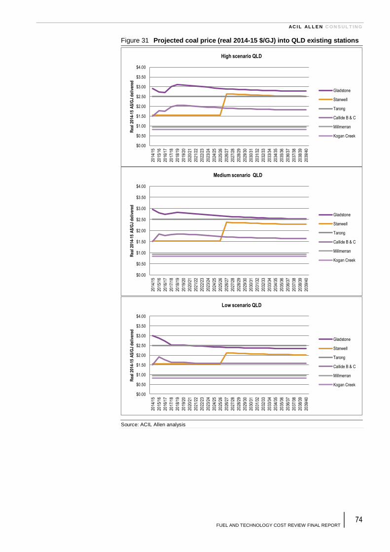
AC I L AL L E N C O N S UL T ING
FUEL AND TECHNOLOGY COST REVIEW FINAL REPORT 74
Figure 31 Projected coal price (real 2014-15 $/GJ) into QLD existing stations
Source: ACIL Allen analysis
$0.00
$0.50
$1.00
$1.50
$2.00
$2.50
$3.00
$3.50
$4.00
2014
/15
2015
/16
2016
/17
2017
/18
2018
/19
2019
/20
2020
/21
2021
/22
2022
/23
2023
/24
2024
/25
2025
/26
2026
/27
2027
/28
2028
/29
2029
/30
2030
/31
2031
/32
2032
/33
2033
/34
2034
/35
2035
/36
2036
/37
2037
/38
2038
/39
2039
/40
Rea
l 20
14-1
5 A
$/G
J d
eliv
ered
High scenario QLD
Gladstone
Stanwell
Tarong
Callide B & C
Millmerran
Kogan Creek
$0.00
$0.50
$1.00
$1.50
$2.00
$2.50
$3.00
$3.50
$4.00
2014
/15
2015
/16
2016
/17
2017
/18
2018
/19
2019
/20
2020
/21
2021
/22
2022
/23
2023
/24
2024
/25
2025
/26
2026
/27
2027
/28
2028
/29
2029
/30
2030
/31
2031
/32
2032
/33
2033
/34
2034
/35
2035
/36
2036
/37
2037
/38
2038
/39
2039
/40
Rea
l 20
14-1
5 A
$/G
J d
eliv
ered
Medium scenario QLD
Gladstone
Stanwell
Tarong
Callide B & C
Millmerran
Kogan Creek
$0.00
$0.50
$1.00
$1.50
$2.00
$2.50
$3.00
$3.50
$4.00
2014
/15
2015
/16
2016
/17
2017
/18
2018
/19
2019
/20
2020
/21
2021
/22
2022
/23
2023
/24
2024
/25
2025
/26
2026
/27
2027
/28
2028
/29
2029
/30
2030
/31
2031
/32
2032
/33
2033
/34
2034
/35
2035
/36
2036
/37
2037
/38
2038
/39
2039
/40
Rea
l 20
14-1
5 A
$/G
J d
eliv
ered
Low scenario QLD
Gladstone
Stanwell
Tarong
Callide B & C
Millmerran
Kogan Creek

AC I L AL L E N C O N S UL T ING
FUEL AND TECHNOLOGY COST REVIEW FINAL REPORT 75
Victorian brown coal and South Australian black coal
Coal mined for power generation in Victoria and South Australia is not suitable for export
and hence removed from fluctuations in export prices.
Extensive deposits of brown coal occur in the tertiary sedimentary basins of Latrobe Valley
coalfield which contains some of the thickest brown coal seams in the world.
Table 32 Coal prices into existing power stations in Qld (Real 2014-15 $/GJ) – High scenario
2014/
15
2015/
16
2016/
17
2017/
18
2018/
19
2019/
20
2020/
21
2021/
22
2022/
23
2023/
24
2024/
25
2025/
26
2026/
27
2027/
28
2028/
29
2029/
30
Gladstone $2.91 $2.73 $2.71 $3.01 $3.10 $3.09 $3.07 $3.04 $3.01 $2.98 $2.95 $2.92 $2.90 $2.88 $2.87 $2.86
Stanwell $1.54 $1.54 $1.54 $1.54 $1.54 $1.54 $1.54 $1.54 $1.54 $1.54 $1.54 $1.54 $2.64 $2.63 $2.61 $2.60
Tarong $2.50 $2.50 $2.50 $2.50 $2.50 $2.50 $2.50 $2.50 $2.50 $2.50 $2.50 $2.50 $2.50 $2.50 $2.50 $2.50
Callide B & C
$1.50 $1.78 $1.77 $1.99 $2.06 $2.05 $2.04 $2.02 $1.99 $1.97 $1.95 $1.93 $1.91 $1.90 $1.89 $1.88
Millmerran $0.94 $0.94 $0.94 $0.94 $0.94 $0.94 $0.94 $0.94 $0.94 $0.94 $0.94 $0.94 $0.94 $0.94 $0.94 $0.94
Kogan Creek
$0.83 $0.83 $0.83 $0.83 $0.83 $0.83 $0.83 $0.83 $0.83 $0.83 $0.83 $0.83 $0.83 $0.83 $0.83 $0.83
Source: ACIL Allen analysis using forecast of thermal coal export prices supplied by AEMO
Table 33 Coal prices into existing power stations in Qld (Real 2014-15 $/GJ) – Medium scenario
2014/
15
2015/
16
2016/
17
2017/
18
2018/
19
2019/
20
2020/
21
2021/
22
2022/
23
2023/
24
2024/
25
2025/
26
2026/
27
2027/
28
2028/
29
2029/
30
Gladstone $2.95 $2.81 $2.73 $2.79 $2.82 $2.80 $2.79 $2.76 $2.74 $2.71 $2.69 $2.66 $2.63 $2.62 $2.61 $2.60
Stanwell $1.54 $1.54 $1.54 $1.54 $1.54 $1.54 $1.54 $1.54 $1.54 $1.54 $1.54 $1.54 $2.38 $2.37 $2.36 $2.35
Tarong $2.50 $2.50 $2.50 $2.50 $2.50 $2.50 $2.50 $2.50 $2.50 $2.50 $2.50 $2.50 $2.50 $2.50 $2.50 $2.50
Callide B & C
$1.50 $1.84 $1.78 $1.82 $1.85 $1.84 $1.83 $1.81 $1.79 $1.77 $1.75 $1.73 $1.71 $1.70 $1.70 $1.69
Millmerran $0.94 $0.94 $0.94 $0.94 $0.94 $0.94 $0.94 $0.94 $0.94 $0.94 $0.94 $0.94 $0.94 $0.94 $0.94 $0.94
Kogan Creek
$0.83 $0.83 $0.83 $0.83 $0.83 $0.83 $0.83 $0.83 $0.83 $0.83 $0.83 $0.83 $0.83 $0.83 $0.83 $0.83
Source: ACIL Allen analysis using forecast of thermal coal export prices supplied by AEMO
Table 34 Coal prices into existing power stations in Qld (Real 2014-15 $/GJ) – Low scenario
2014/
15
2015/
16
2016/
17
2017/
18
2018/
19
2019/
20
2020/
21
2021/
22
2022/
23
2023/
24
2024/
25
2025/
26
2026/
27
2027/
28
2028/
29
2029/
30
Gladstone $2.99 $2.88 $2.71 $2.53 $2.52 $2.52 $2.50 $2.48 $2.45 $2.44 $2.42 $2.41 $2.40 $2.39 $2.39 $2.38
Stanwell $1.54 $1.54 $1.54 $1.54 $1.54 $1.54 $1.54 $1.54 $1.54 $1.54 $1.54 $1.54 $2.11 $2.10 $2.09 $2.08
Tarong $2.50 $2.50 $2.50 $2.50 $2.50 $2.50 $2.50 $2.50 $2.50 $2.50 $2.50 $2.50 $2.50 $2.50 $2.50 $2.50
Callide B & C
$1.50 $1.90 $1.77 $1.64 $1.63 $1.63 $1.61 $1.60 $1.58 $1.58 $1.58 $1.58 $1.58 $1.58 $1.58 $1.58
Millmerran $0.94 $0.94 $0.94 $0.94 $0.94 $0.94 $0.94 $0.94 $0.94 $0.94 $0.94 $0.94 $0.94 $0.94 $0.94 $0.94
Kogan Creek
$0.83 $0.83 $0.83 $0.83 $0.83 $0.83 $0.83 $0.83 $0.83 $0.83 $0.83 $0.83 $0.83 $0.83 $0.83 $0.83
Source: ACIL Allen analysis using forecast of thermal coal export prices supplied by AEMO

AC I L AL L E N C O N S UL T ING
FUEL AND TECHNOLOGY COST REVIEW FINAL REPORT 76
Mine mouth dedicated coalmines supply all the power stations. The coalmines are owned by
the same entities that own the power stations with two exceptions. The exceptions are the
Loy Yang B power station, where the mine, which is in close proximity to the power station,
is owned and operated by Loy Yang Power, the owners and operators of the Loy Yang A
power station and Energy Brix which is supplied by Morwell mine.
The marginal price of coal for the Victorian power stations is generally taken as the marginal
cash costs of mining the coal.
The only currently producing coalfield in South Australia is at Leigh Creek based on low-
grade sub-bituminous coal. The mining operation involves drilling, blasting and removal of
overburden and coal by shovels and trucks. After mining, the crushed coal is railed to the
Port Augusta power stations. The Leigh Creek mine is about 250 km from the power
stations. A long-term rail haulage contract is in place with Pacific National.
Figure 32 Projected coal price (real 2014-15 $/GJ) into VIC and SA existing
stations
Source: ACIL Allen analysis
$0.00
$0.50
$1.00
$1.50
$2.00
$2.50
$3.00
$3.50
$4.00
2014
/15
2015
/16
2016
/17
2017
/18
2018
/19
2019
/20
2020
/21
2021
/22
2022
/23
2023
/24
2024
/25
2025
/26
2026
/27
2027
/28
2028
/29
2029
/30
2030
/31
2031
/32
2032
/33
2033
/34
2034
/35
2035
/36
2036
/37
2037
/38
2038
/39
2039
/40
Rea
l 20
14-1
5 A
$/G
J d
eliv
ered
All scenarios VIC and SA
Yallourn
Loy Yang A
Loy Yang B
Hazelwood
Anglesea
Energy Brix
Northern
Table 35 Coal prices into existing power stations in Victoria and SA (Real 2014-15 $/GJ) – All scenarios
2014/
15
2015/
16
2016/
17
2017/
18
2018/
19
2019/
20
2020/
21
2021/
22
2022/
23
2023/
24
2024/
25
2025/
26
2026/
27
2027/
28
2028/
29
2029/
30
Yallourn $0.10 $0.10 $0.10 $0.11 $0.11 $0.11 $0.11 $0.11 $0.12 $0.12 $0.12 $0.12 $0.13 $0.13 $0.13 $0.13
Loy Yang A $0.09 $0.09 $0.09 $0.09 $0.10 $0.10 $0.10 $0.10 $0.10 $0.11 $0.11 $0.11 $0.11 $0.12 $0.12 $0.12
Loy Yang B $0.40 $0.40 $0.40 $0.41 $0.41 $0.42 $0.42 $0.42 $0.43 $0.43 $0.44 $0.44 $0.45 $0.45 $0.45 $0.46
Hazelwood $0.09 $0.09 $0.09 $0.09 $0.10 $0.10 $0.10 $0.10 $0.10 $0.11 $0.11 $0.11 $0.11 $0.12 $0.12 $0.12
Anglesea $0.43 $0.43 $0.43 $0.44 $0.44 $0.45 $0.45 $0.46 $0.46 $0.47 $0.47 $0.47 $0.48 $0.48 $0.49 $0.49
Energy Brix $0.64 $0.65 $0.66 $0.66 $0.67 $0.68 $0.68 $0.69 $0.70 $0.70 $0.71 $0.72 $0.72 $0.73 $0.74 $0.75
Northern $1.64 $1.68 $1.71 $1.74 $2.29 $2.34 $2.39 $2.43 $2.48 $2.53 $2.58 $2.63 $2.69 $2.74 $2.80 $2.85
Source: ACIL Allen analysis using forecast of thermal coal export prices supplied by AEMO
AC I L AL L E N C O N S UL T ING
FUEL AND TECHNOLOGY COST REVIEW FINAL REPORT 77
7.4 Price of coal into new power stations by zone
For new stations ACIL Allen undertook and analysis of known coal deposits in the 17 zones
and selected those zones where adequate coal resources were available to support at least
2000 MW of future coal fired generation. Only seven of the 17 zones were judged as having
adequate coal resources and they were NQ, CQ and SWQ in Queensland NCEN, NNS and
SWNSW in New South Wales and LV in Victoria.
The price of black coal in each zone in Queensland and New South Wales was based on
the deposit found to have the lowest delivered cost to a power station located close to the
transmission network in that zone. For each black coal deposit the delivered price of coal
was taken as the maximum of the cost of production and export parity value.
For Victoria the delivered price of brown coal is assumed at the cash cost of production
which is forecast to increase at between 1 and 2 percent.
The real coal prices forecast in each of the seven zones are shown in Figure 33. Costs
variation between the zones is due to the quality of the available deposits and whether
access to export markets is expected to be available. The influence of export markets is
evident in the prices in CQ, NNS and NCEN. The prices in other zones are linked to mining
costs.

AC I L AL L E N C O N S UL T ING
FUEL AND TECHNOLOGY COST REVIEW FINAL REPORT 78
Figure 33 Coal prices into new power stations by zone (Real 2014-15 $/GJ)
Source: ACIL Allen analysis using forecast of thermal coal export prices supplied by AEMO
$0.00
$0.50
$1.00
$1.50
$2.00
$2.50
$3.00
$3.50
real
201
4/15
A$/
GJ
High NQ
CQ
SWQ
NNS
NCEN
SWNSW
LV
$0.00
$0.50
$1.00
$1.50
$2.00
$2.50
$3.00
$3.50
real
201
4/15
A$/
GJ
Medium NQ
CQ
SWQ
NNS
NCEN
SWNSW
LV
$0.00
$0.50
$1.00
$1.50
$2.00
$2.50
$3.00
$3.50
real
201
4/15
A$/
GJ
Low NQ
CQ
SWQ
NNS
NCEN
SWNSW
LV
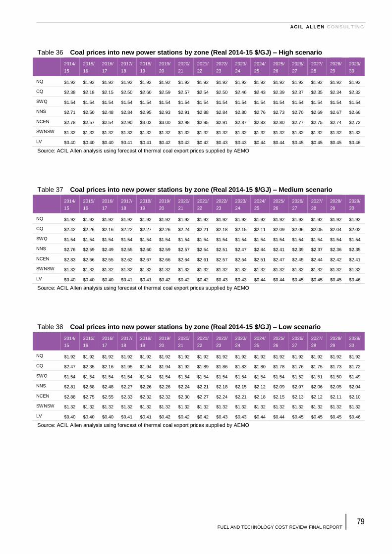
AC I L AL L E N C O N S UL T ING
FUEL AND TECHNOLOGY COST REVIEW FINAL REPORT 79
Table 36 Coal prices into new power stations by zone (Real 2014-15 $/GJ) – High scenario
2014/
15
2015/
16
2016/
17
2017/
18
2018/
19
2019/
20
2020/
21
2021/
22
2022/
23
2023/
24
2024/
25
2025/
26
2026/
27
2027/
28
2028/
29
2029/
30
NQ $1.92 $1.92 $1.92 $1.92 $1.92 $1.92 $1.92 $1.92 $1.92 $1.92 $1.92 $1.92 $1.92 $1.92 $1.92 $1.92
CQ $2.38 $2.18 $2.15 $2.50 $2.60 $2.59 $2.57 $2.54 $2.50 $2.46 $2.43 $2.39 $2.37 $2.35 $2.34 $2.32
SWQ $1.54 $1.54 $1.54 $1.54 $1.54 $1.54 $1.54 $1.54 $1.54 $1.54 $1.54 $1.54 $1.54 $1.54 $1.54 $1.54
NNS $2.71 $2.50 $2.48 $2.84 $2.95 $2.93 $2.91 $2.88 $2.84 $2.80 $2.76 $2.73 $2.70 $2.69 $2.67 $2.66
NCEN $2.78 $2.57 $2.54 $2.90 $3.02 $3.00 $2.98 $2.95 $2.91 $2.87 $2.83 $2.80 $2.77 $2.75 $2.74 $2.72
SWNSW $1.32 $1.32 $1.32 $1.32 $1.32 $1.32 $1.32 $1.32 $1.32 $1.32 $1.32 $1.32 $1.32 $1.32 $1.32 $1.32
LV $0.40 $0.40 $0.40 $0.41 $0.41 $0.42 $0.42 $0.42 $0.43 $0.43 $0.44 $0.44 $0.45 $0.45 $0.45 $0.46
Source: ACIL Allen analysis using forecast of thermal coal export prices supplied by AEMO
Table 37 Coal prices into new power stations by zone (Real 2014-15 $/GJ) – Medium scenario
2014/
15
2015/
16
2016/
17
2017/
18
2018/
19
2019/
20
2020/
21
2021/
22
2022/
23
2023/
24
2024/
25
2025/
26
2026/
27
2027/
28
2028/
29
2029/
30
NQ $1.92 $1.92 $1.92 $1.92 $1.92 $1.92 $1.92 $1.92 $1.92 $1.92 $1.92 $1.92 $1.92 $1.92 $1.92 $1.92
CQ $2.42 $2.26 $2.16 $2.22 $2.27 $2.26 $2.24 $2.21 $2.18 $2.15 $2.11 $2.09 $2.06 $2.05 $2.04 $2.02
SWQ $1.54 $1.54 $1.54 $1.54 $1.54 $1.54 $1.54 $1.54 $1.54 $1.54 $1.54 $1.54 $1.54 $1.54 $1.54 $1.54
NNS $2.76 $2.59 $2.49 $2.55 $2.60 $2.59 $2.57 $2.54 $2.51 $2.47 $2.44 $2.41 $2.39 $2.37 $2.36 $2.35
NCEN $2.83 $2.66 $2.55 $2.62 $2.67 $2.66 $2.64 $2.61 $2.57 $2.54 $2.51 $2.47 $2.45 $2.44 $2.42 $2.41
SWNSW $1.32 $1.32 $1.32 $1.32 $1.32 $1.32 $1.32 $1.32 $1.32 $1.32 $1.32 $1.32 $1.32 $1.32 $1.32 $1.32
LV $0.40 $0.40 $0.40 $0.41 $0.41 $0.42 $0.42 $0.42 $0.43 $0.43 $0.44 $0.44 $0.45 $0.45 $0.45 $0.46
Source: ACIL Allen analysis using forecast of thermal coal export prices supplied by AEMO
Table 38 Coal prices into new power stations by zone (Real 2014-15 $/GJ) – Low scenario
2014/
15
2015/
16
2016/
17
2017/
18
2018/
19
2019/
20
2020/
21
2021/
22
2022/
23
2023/
24
2024/
25
2025/
26
2026/
27
2027/
28
2028/
29
2029/
30
NQ $1.92 $1.92 $1.92 $1.92 $1.92 $1.92 $1.92 $1.92 $1.92 $1.92 $1.92 $1.92 $1.92 $1.92 $1.92 $1.92
CQ $2.47 $2.35 $2.16 $1.95 $1.94 $1.94 $1.92 $1.89 $1.86 $1.83 $1.80 $1.78 $1.76 $1.75 $1.73 $1.72
SWQ $1.54 $1.54 $1.54 $1.54 $1.54 $1.54 $1.54 $1.54 $1.54 $1.54 $1.54 $1.54 $1.52 $1.51 $1.50 $1.49
NNS $2.81 $2.68 $2.48 $2.27 $2.26 $2.26 $2.24 $2.21 $2.18 $2.15 $2.12 $2.09 $2.07 $2.06 $2.05 $2.04
NCEN $2.88 $2.75 $2.55 $2.33 $2.32 $2.32 $2.30 $2.27 $2.24 $2.21 $2.18 $2.15 $2.13 $2.12 $2.11 $2.10
SWNSW $1.32 $1.32 $1.32 $1.32 $1.32 $1.32 $1.32 $1.32 $1.32 $1.32 $1.32 $1.32 $1.32 $1.32 $1.32 $1.32
LV $0.40 $0.40 $0.40 $0.41 $0.41 $0.42 $0.42 $0.42 $0.43 $0.43 $0.44 $0.44 $0.45 $0.45 $0.45 $0.46
Source: ACIL Allen analysis using forecast of thermal coal export prices supplied by AEMO


