m FILE COPJf ^ USAAEFA PROJECT NO. 81-01-6 US ARMY AVIATION SYSTEMS COMMAND FUEL CONSERVATION EVALUATION OF US ARMY HELICOPTERS PART 6, PERFORMANCE CALCULATOR EVALUATION IT) (D 00 < I D < E F A FLOYD DOMINICK PROJECT OFFICER/ENGINEER ROY A. LOCKWOOD MAJ, AV PROJECT PILOT JULY 1986 FINAL REPORT APPROVED FOR PUBLIC RELEASE. DISTRIBUTION UNLIMITED. US ARMY AVIATION ENGINEERING FLIGHT ACTIVITY EDWARDS AIR FORCE BASE, CALIFORNIA 93523 • 5000
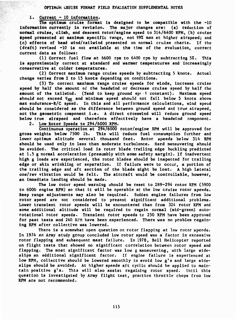
Transcript
m FILE COPJf ^
USAAEFA PROJECT NO. 81-01-6
US ARMY AVIATION SYSTEMS COMMAND
FUEL CONSERVATION EVALUATION OF US ARMY HELICOPTERS PART 6, PERFORMANCE CALCULATOR EVALUATION
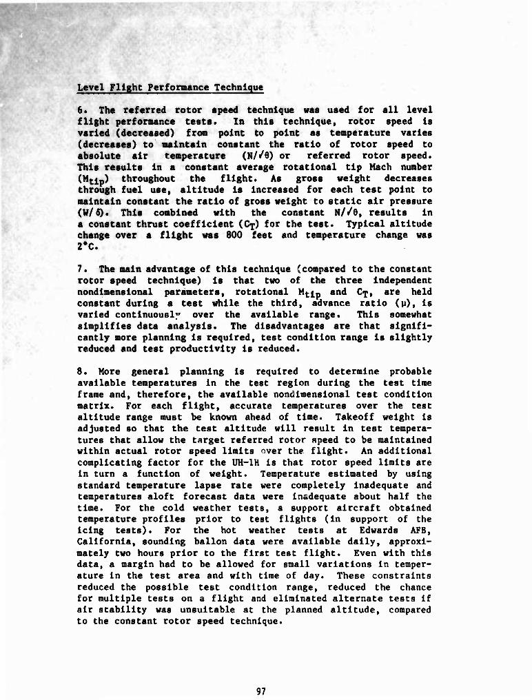
IT)
(D
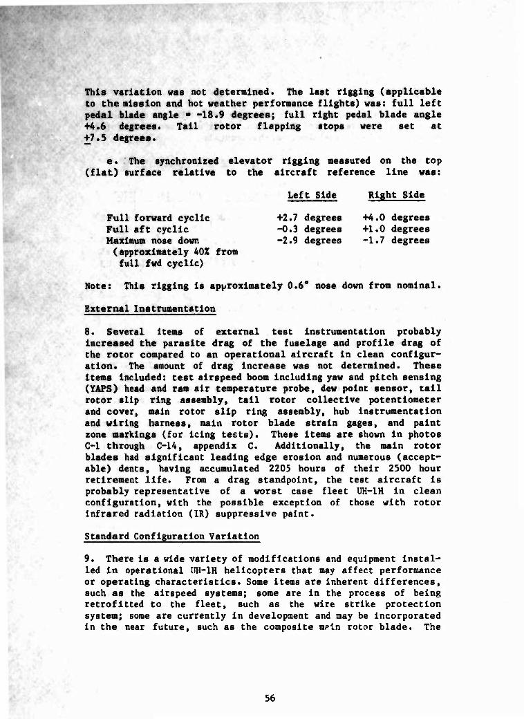
00
<
I D <
E F A
FLOYD DOMINICK PROJECT OFFICER/ENGINEER
ROY A. LOCKWOOD MAJ, AV
PROJECT PILOT
JULY 1986
FINAL REPORT
APPROVED FOR PUBLIC RELEASE. DISTRIBUTION UNLIMITED.
US ARMY AVIATION ENGINEERING FLIGHT ACTIVITY EDWARDS AIR FORCE BASE, CALIFORNIA 93523 • 5000
DISCLAIMER NOTICE
The findings of this report are not to be comtmed as an official Department of the Army position inUeas to deognated by other authorized documents.
DISPOSITION INSTRUCTIONS
Destroy this report when it is no longer needed. Do not return it to the originator.
TRADE NAMES
The use of trade names in this report does not constitute an official endorsement or approval of the use of the commercial hardware and software.
UNCLASSIFIED SKCURITY CLASH PIC ATION OP THIS PAGE (Wh— Oat» Bnfnd)
I. HUoftf NUM4IK REPORT DOCUMENTATION PAGE
a. OOVT Acci
USAAEFA PROJECT NO. 81-01-6 Ai&~A\
READ I STRUCTIONS BEFORE COMPLETING FORM
ä .*■ RCCIPICNT'S CATALOG NUMSKR
4. TITLE fa* SuMM*>
FUEL CONSERVATION OF US ARMY HELICOPTERS PART 6, PERFORMANCE CALCULATOR EVALUATION
8. TYPE OP REPORT • PtRIOD COVERED
FINAL JANUARY 1981 «. PERPORMING ORG. REPORT NUMSEN
r. AUTHONT*) FLOYD DOMINICK, ROY A. LOCKWOOD
• ■ CONTRACT OR GRANT NUMBERf»)
tO. PROGRAM ELEMENT, PROJECT, TASK AREA » WORK UNIT NUMBERS
t. ^IRPONMINOOROANIZATION NAME AND ADDRESS
US ARMY AVN ENGINEERING fllCHT ACTIVITY EDWARDS AIR FORCE BASE, CA 93523-5000
II. CONTROLLING OPPICE NAME AND ADDRESS
US ARMY AVIATION SYSTEMS COMMAND 4300 GOODFELLOW BOULEVARD ST. LOUIS, MO 63120-1798 I«. MONITORING AGENCV NAME • AODRESSC" ällHtmtl Inm ConlroUInt Ollle»)
12. REPORT DATE
JULY 1986 IS. NUMBER OP PAGES
208 IS. SECURITY CLASS, (el Ma
UNCLASSIFIED
in DECLASSIPICATION/OOWNORAOING SCHEDULE
K DISTRISUTION STATEMENT (•! «I« R« *t) ""
Approved for public release; distribution unlimited.
IT. OIITRIBUTIOH STATEMENT (ol (ha «6«lracl mtffd In Block tO. II dlllwmtl «ran Rmpott) £& m^ IB. SUPPLEMENTARY NOTES
f
IB. KEY WORDS (Cenllnum on rmnta» «Ida II nacaaaarr anrf Idanllly by block numbor) ,
•- Conpressibiltiy Ef fects y Level Flighr and Hdver Data, f Flight Management Calculator. Regressive Analog Model
Flight Planning DH-1H Ä- Fuel Saving \|
^5 t*. ABSTRACT fTHitfciii ommwmm o»* M nmo—atf m* UonlHr by blockmmtbt)
he US Army Aviation Engineering Flight Activity conducted an evaluation of Flight Management Calculator for the UH-1H. The calculator was a Hewlett-Packard HP-41CV. The performance calculator was evaluated for flight planning and in-flight use during U mission flights simulating operational conditions. The calculator was much easier to use in-flight than the operator's manual data. The calculator program needs improvement in the areas of pre-flight planning and execution speed. The mission flights demonstrated a 19 percent.
:K
UR\«lili09xr Lau
tCUWITY CLAMIFICATIOW Or THU PAQUOmm Dm»
fuel saving using "optimus" over "normal" flight profiles In warm temperatures (IS degrees C above standard). Savings would be greater at colder temperatures because of Increasing compressibility effects. Acceptable accuracy for Indiv- idual aircraft under operational conditions may require a regressive analog model in which Individual aircraft data are used to update the program. The perforsance data base for the UH-1H was expanded with level flight and hover data to thrust coefficients and Mach numbers to the practical limits of aircraft operation. __^ fir^ AMA. ^
u?tr^ution/_
'DlBt
UNCLASSIFIED
IICUMITV CLAMIPICATION OP THIS PlOKWhin Oat« Bnfnd)
TABLE OF CONTENTS
INTRODUCTION
Background Test Objectives Description
Aircraft Flight Management Calculator
Test Scope Test Methodology
Page
2 5
RESULTS AND DISCUSSION
General 6 Calculator Evaluation 6
Pilot Comments 8 Documentation 9 Physical Characteristics 10 Accuracy • 10 Units - Conversions 12 Data Ranges 12 Data Limits 12 Input 13 Output 14 Specific Performance Comments 15
Weight and Balance 13 Ground Operations 16 Engine Performance 17 Hover 17 Takeoff 17 Climb - Descent 18 Winds and Temperature 18 Emergency Performance 18
Future Development 19 Mission Flights 20
General 20 Flight Conditions 21
Loading and Fuel Quantity 23 Cruise Conditions 24
Cruise Altitude and Temperature 24 Cruise Rotor Speed 24 Cruise Airspeed 23
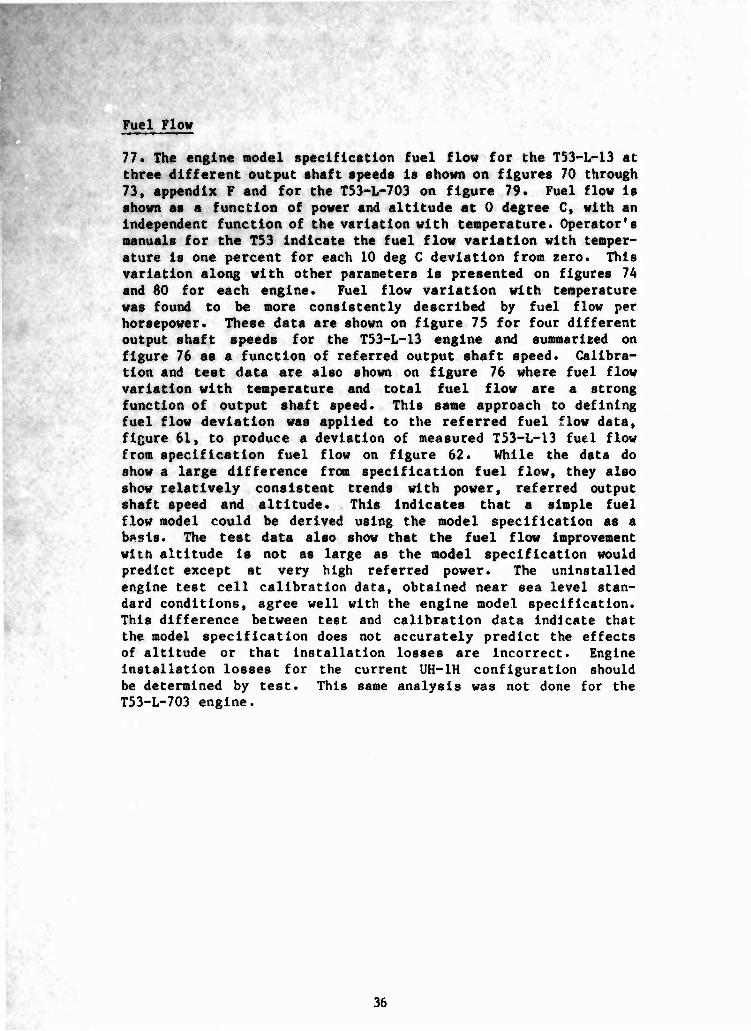
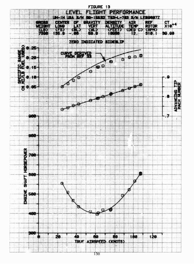
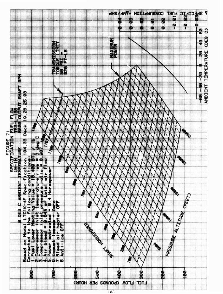
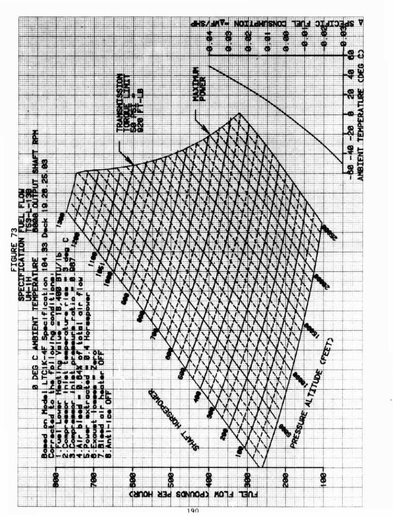
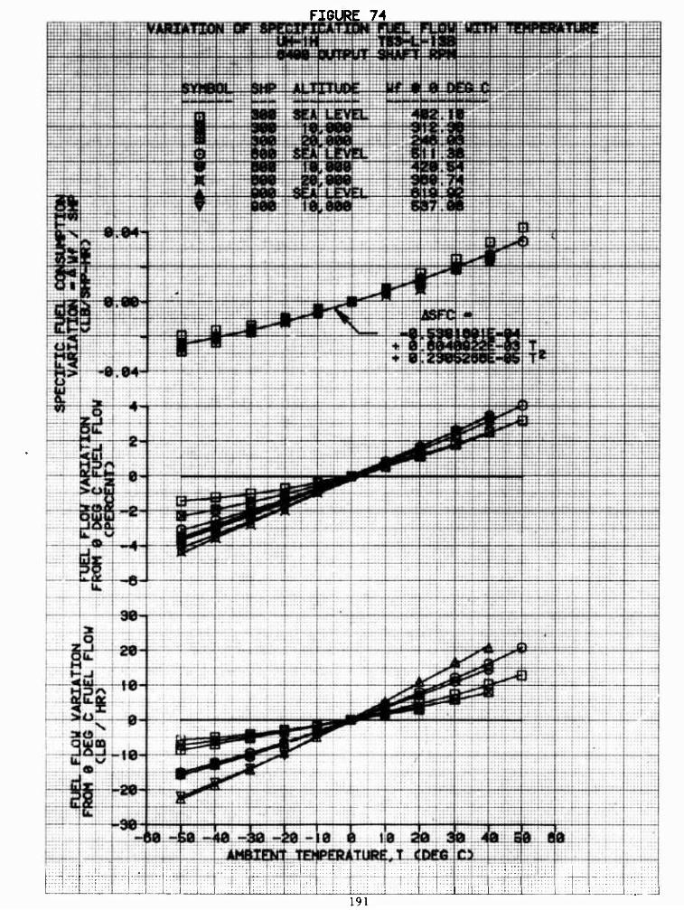
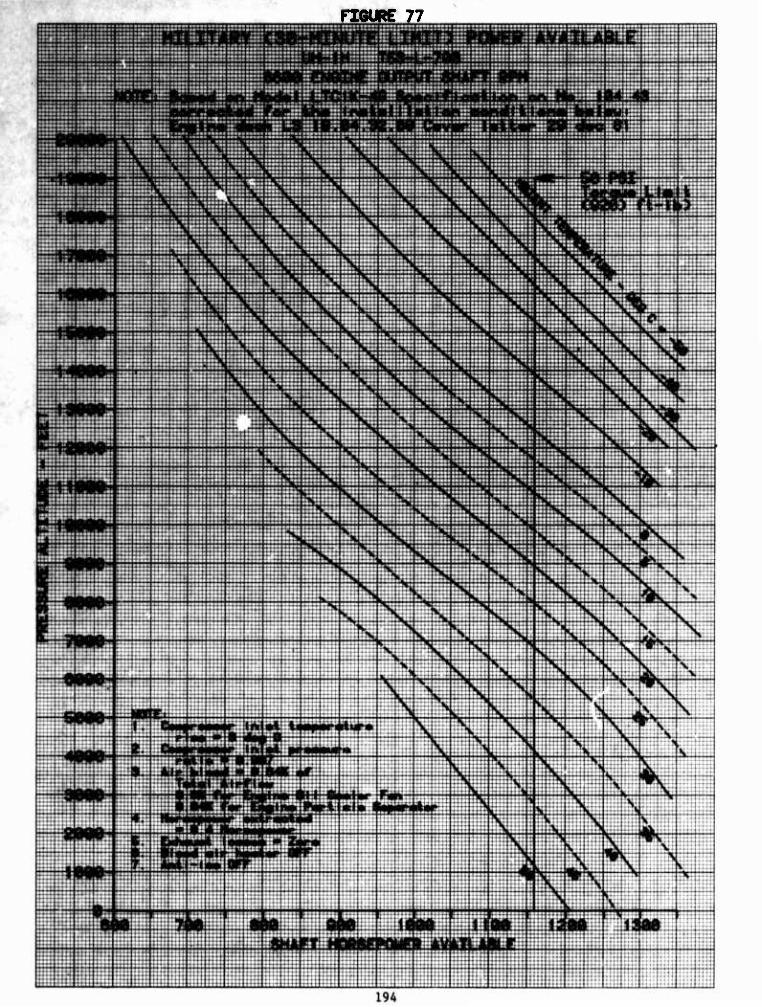
Performance Tests 34 Level Flight Performance 34 Hover Performance 35 Engine Characteristics 35 Power Available 35 Fuel Flow 36
CONCLUSIONS
General 37 Specific 37
RECOMMENDATIONS AO
APPENDIXES
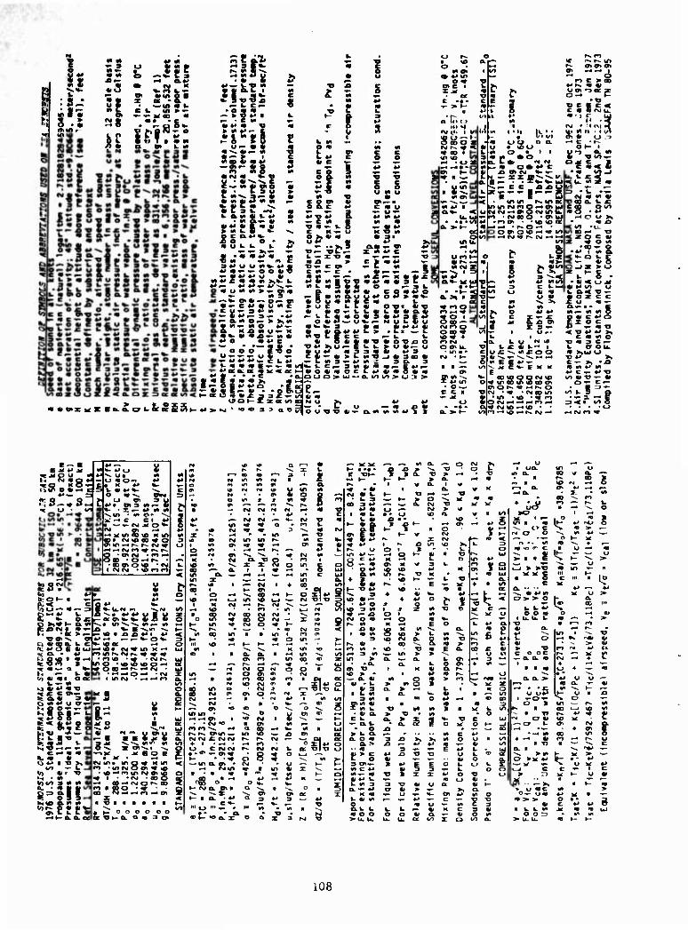
A. References 42 B. Flight Management Calculator and Aircraft Description.. 45 C. Test Instrumentation 62 D. Test Techniques and Data Analysis Methods 95 E. Prototype Optimum Cruise Charts and Supplemental
Notes Ill F. Graphical Test Data 117
DISTRIBUTION
I
INTRODUCTION
BACKCROUND
1. The US Army is placing emphasis on achieving fuel conservation In operation of Army aircraft. The Department of the Army, Deputy Chief of Staff for Logistics (DCSLOG), Aviation Logistics Office/Special Assistant supports a program to minimize fuel consumption. The Directorate for Engineering, US Army Aviation Systems Commaml (AVSCOM) and US Army Aviation Engineering Flight Activity (USAAEZA), Jointly developed a fuel conservation program which both US Army Materiel Command and DCSLOG agreed to imple- ment. USAAEFA began a five part flight test program In January 1981. Results are reported in references 1 through 5, appendix A. Concurrently, AVSCOM contracted Bell Helicopter Textron (BHT) to develop a software program for the Hewlett-Packard HP-4ICV calculator which could be used by Army pilots to provide perfor- mance data and fuel consumption data during operational missions. This calculator program and results of a limited field evaluation are reported in reference 6. AVSCOM requested that USAAEFA conduct an engineering flight evaluation of the performance calculator and provide additional performance data for the UH-1H to complete the perfor lance characterization for the fuel conservation effort (ref 7). A test plan (ref 8) was prepared In response to that request.
TEST OBJECTIVES
2. The objectives of this test were to evaluate the overall adequacy of the performance calculator, determine optimum cruise fuel savings under operational conditions and to obtain additional blade compressibility and blade stall flight test data on the UH-IH to complete the performance characterization for the fuel conservation effort.
DESCRIPTION
Aircraft
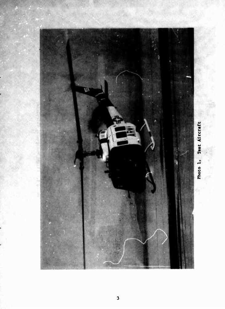
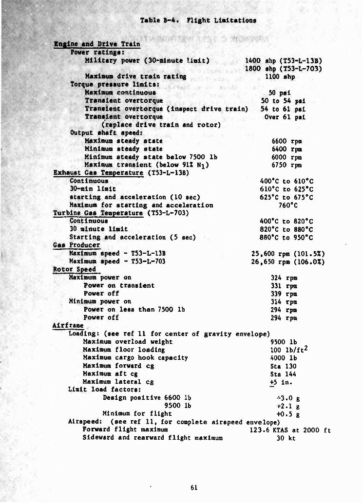
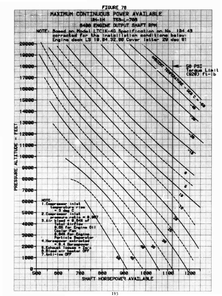
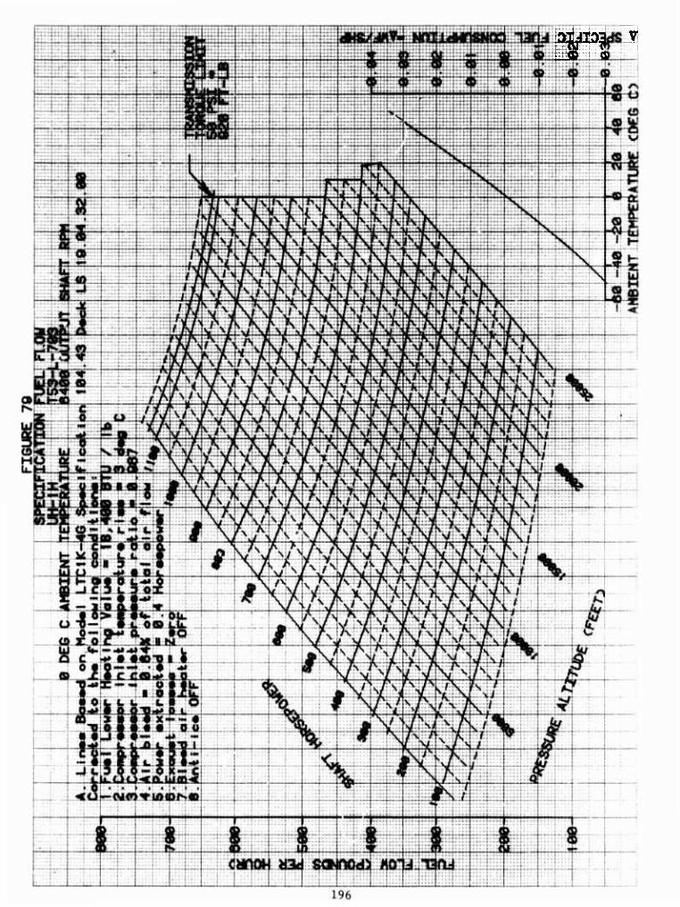
3. The UH-IH is a thirteen-place, single engine helicopter with a 9500 pound (lb) maximum gross weight. Lift is provided by a two- bladed, 48-foot diameter, teetering main rotor. A two-bladed pusher type tall rotor provides antitorque and directional con- trol. Power is normally supplied by a T53-L-13B free turbine engine rated at 1400 horsepower. For part of these tests a TS3-L-703 engine with a thermodynamic rating of 1800 horsepower was used. This engine has been designated as a contingency engine for the UH-IH. Drive train limits derate either engine
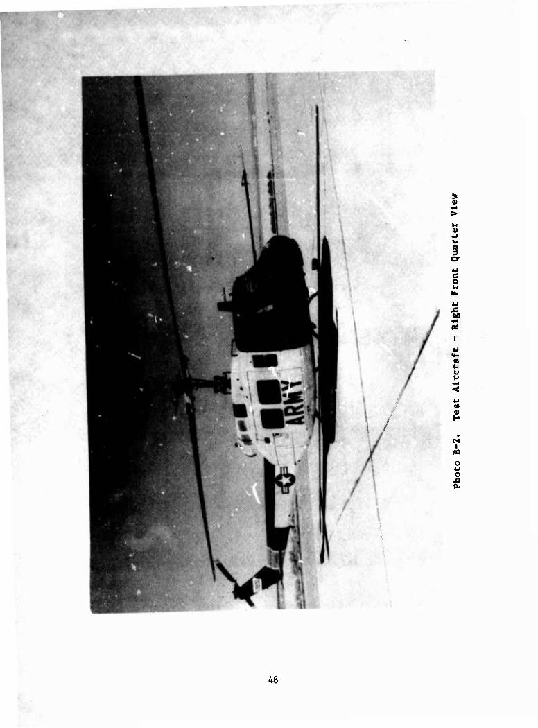
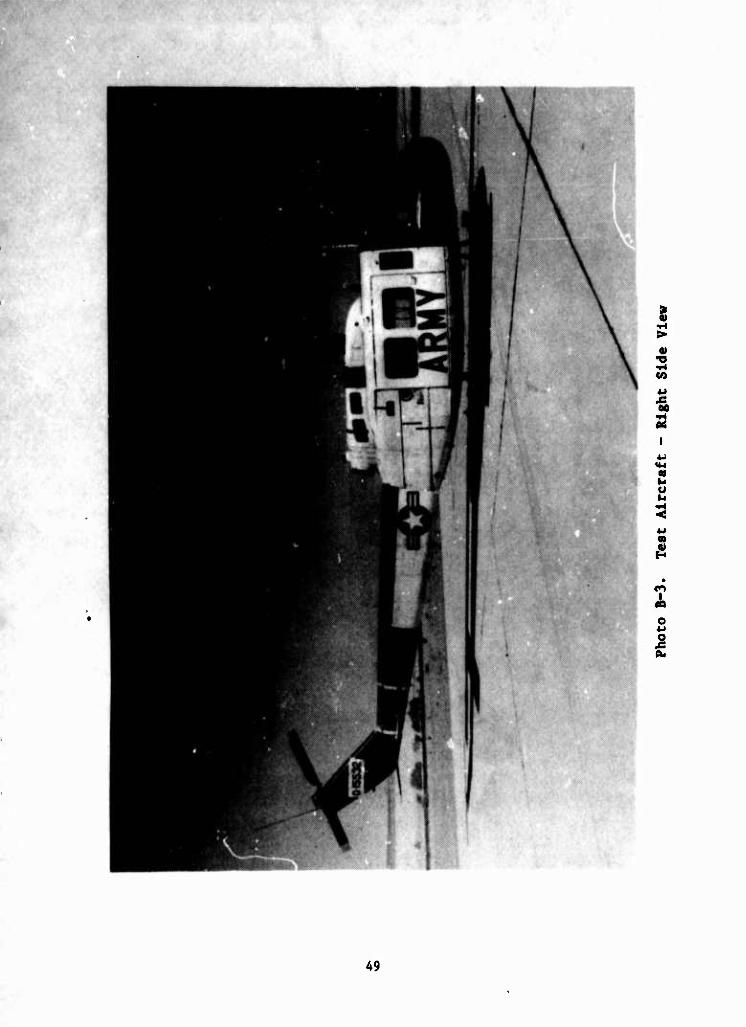
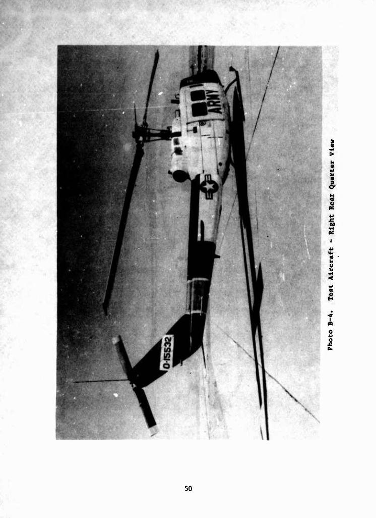
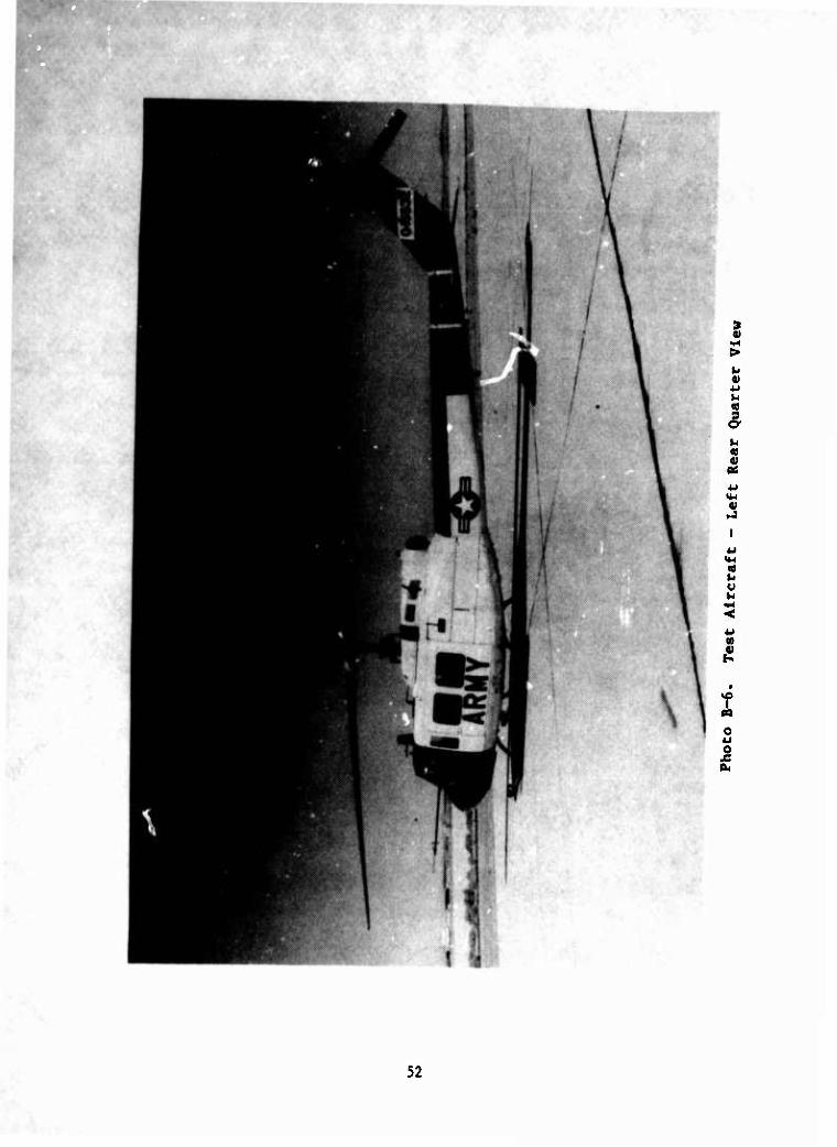
to 1100 horsepower, which is available up to 7000 feet and 15,000 feet at standard temperatures from the -13B and -703 engines respectively. The test aircraft (photo 1), US Army serial number 69-15532, is a standard production UH-1H. A more complete descrip- tion Is presented in appendix B. Additional information can be found in the operator's manuals (refs 9, 10 and 11, app A) and the detail specification (ref 12). The aircraft was in normal clean configuration except for the test instrumentation described in appendix C.
Flight Management Calculator
4. The Flight Management Calculator (FMC) consists of a Hewlett- Packard HP-41CV programmable scientific pocket calculator, BHT modification hardware and Performance Data Quick (PDQ) software. The FMC as configured by BHT for the calculator evaluation is shown In photograph 2. The modifications to the HP-41CV expanded the capability of the basic calculator, provided the pilot with input function labels and allowed attachment to the pilot's knee board. The PDQ program provides weight and balance information as well as performance information for various flight conditions. The program is considered proprietary by BHT and was programmed in "private" mode which makes it inaccessible. References 6 and 13, appendix A and appendix B provide thorough documentation and description of the FMC.
TEST SCOPE
5. Fourteen mission flights were conducted to determine optimum cruise fuel savings and evaluate the FMC. All tests were within the operator's manual limitations as amended by the airworthiness release (ref 14, app A), which allowed a maximum takeoff weight of 10,000 lb (300 lb over the normal limit) and rotor speeds down to 304 rpm below 8000 lb gross weight and 294 rpm below 7300 lb gross weight. These flights covered a spectrum of UH-1H range capabilities, air traffic control constraints, weather conditions, and other operational variables. Mission test flights were conducted with a mid center of gravity (eg) and a nominal engine
I start weight of 8100 pounds, which represented full fuel, a crew of two, and 1000 lb cargo or passengers. Comparative mission flights using "normal" and "optimum" flight profiles gave an approximation of fuel savings using optimum conditions. Cruise altitudes were nominally 1300 feet above ground level (AGL) for the normal flight profiles. Cruise altitude, rotor speed, and airspeed for the optimum flight profiles were determined from previous test data (ref 2, app A) included in appendix E.
u o u
«0
H
o tu
u o
3 o (0 o
a
00
s 4J
00
<M
o Or
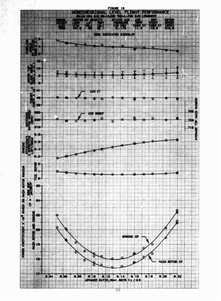
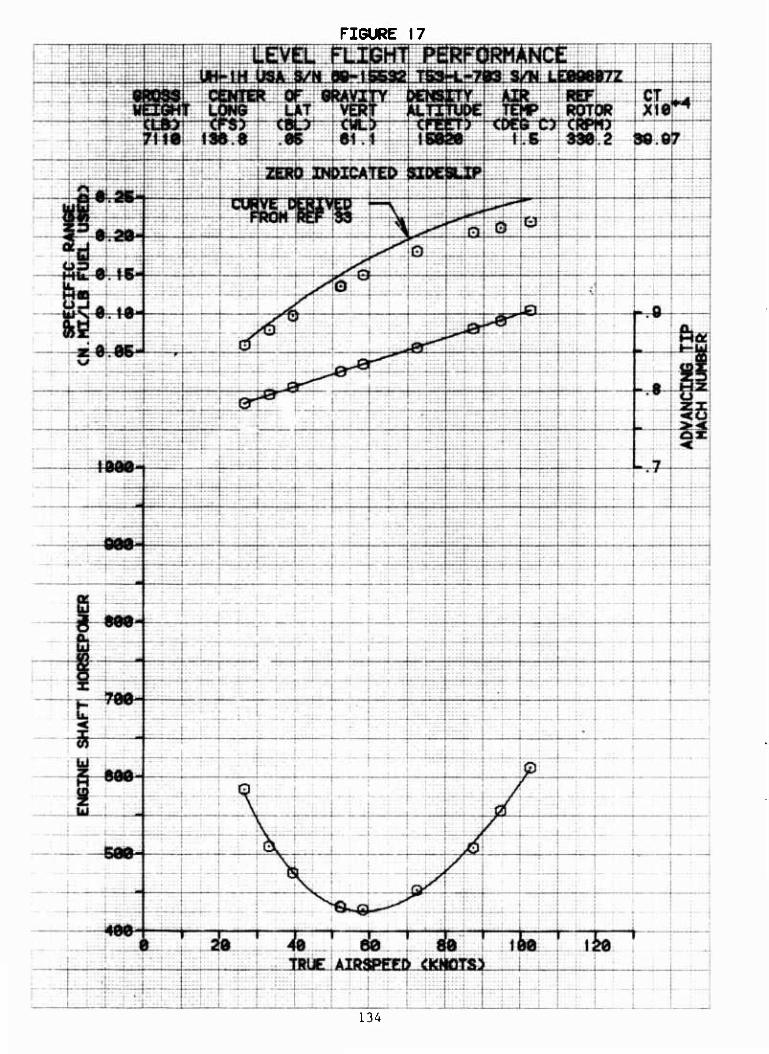
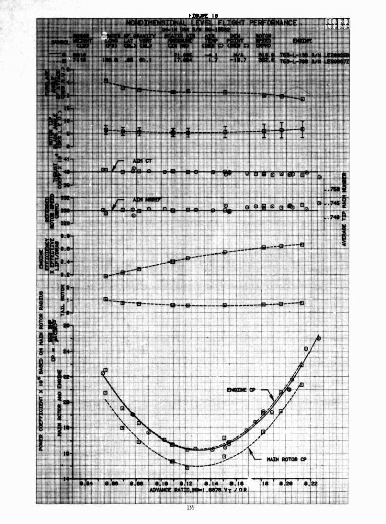
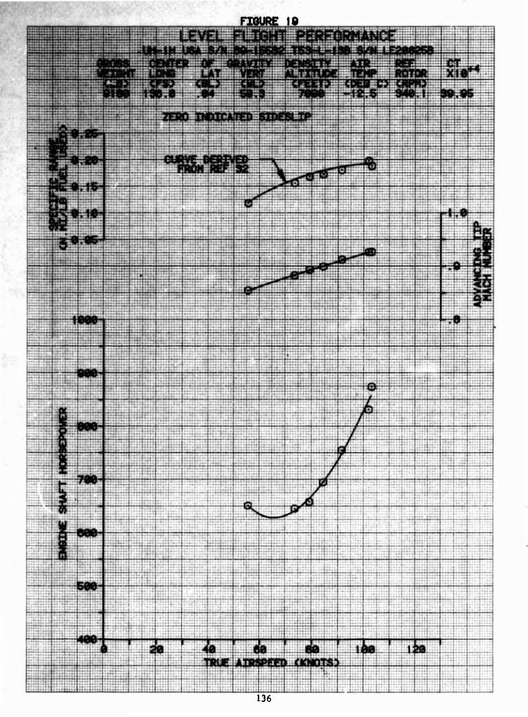
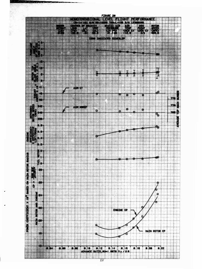
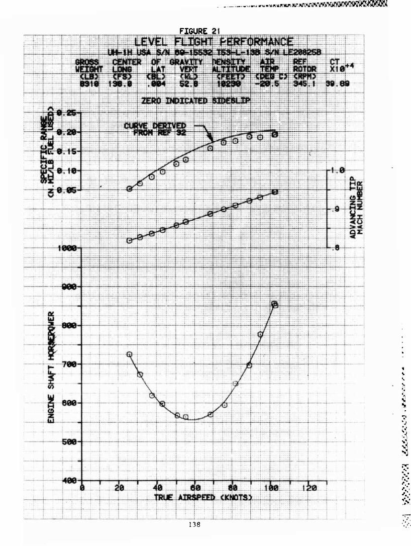
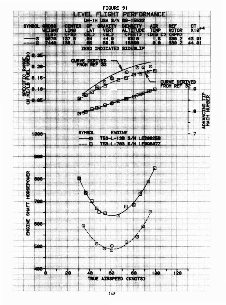
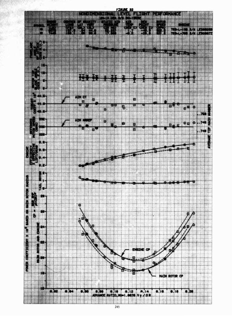
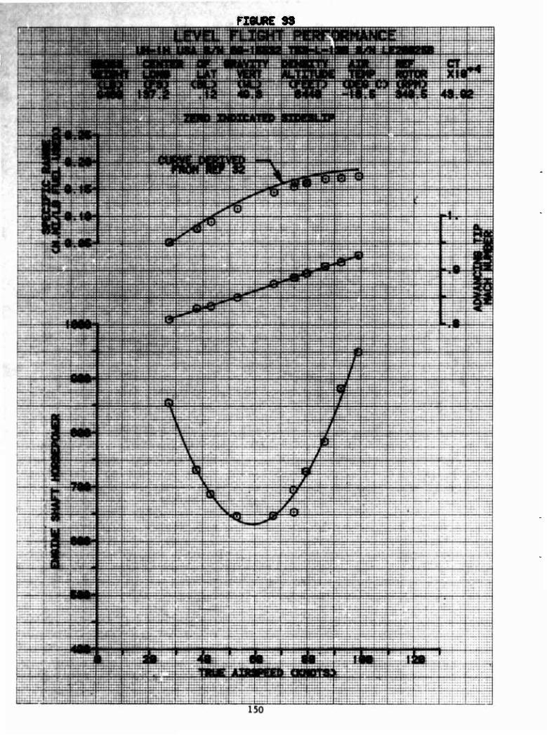
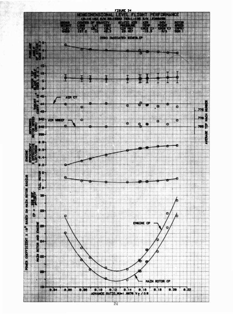
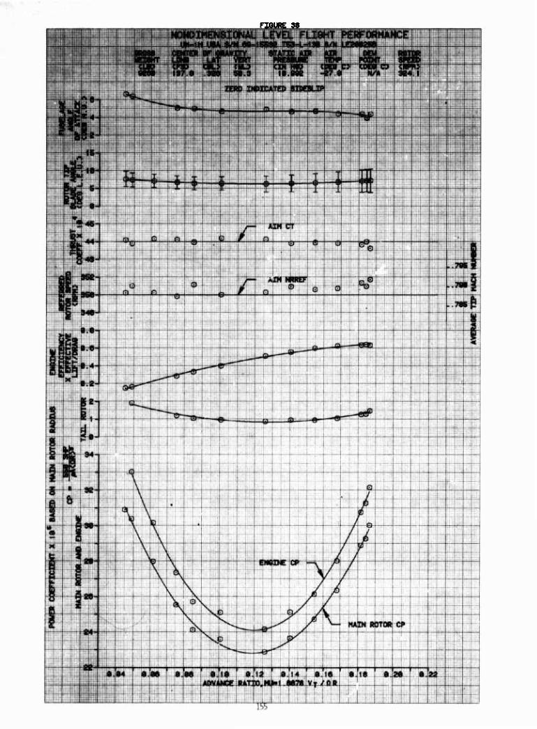
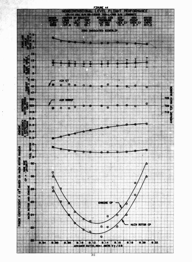
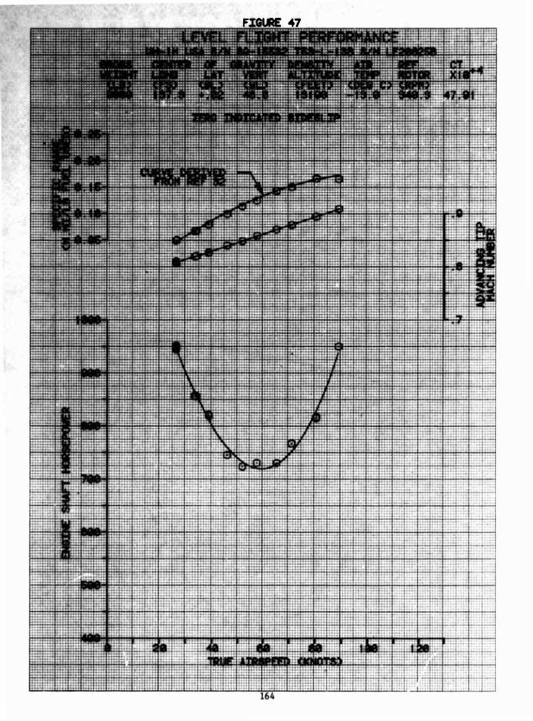
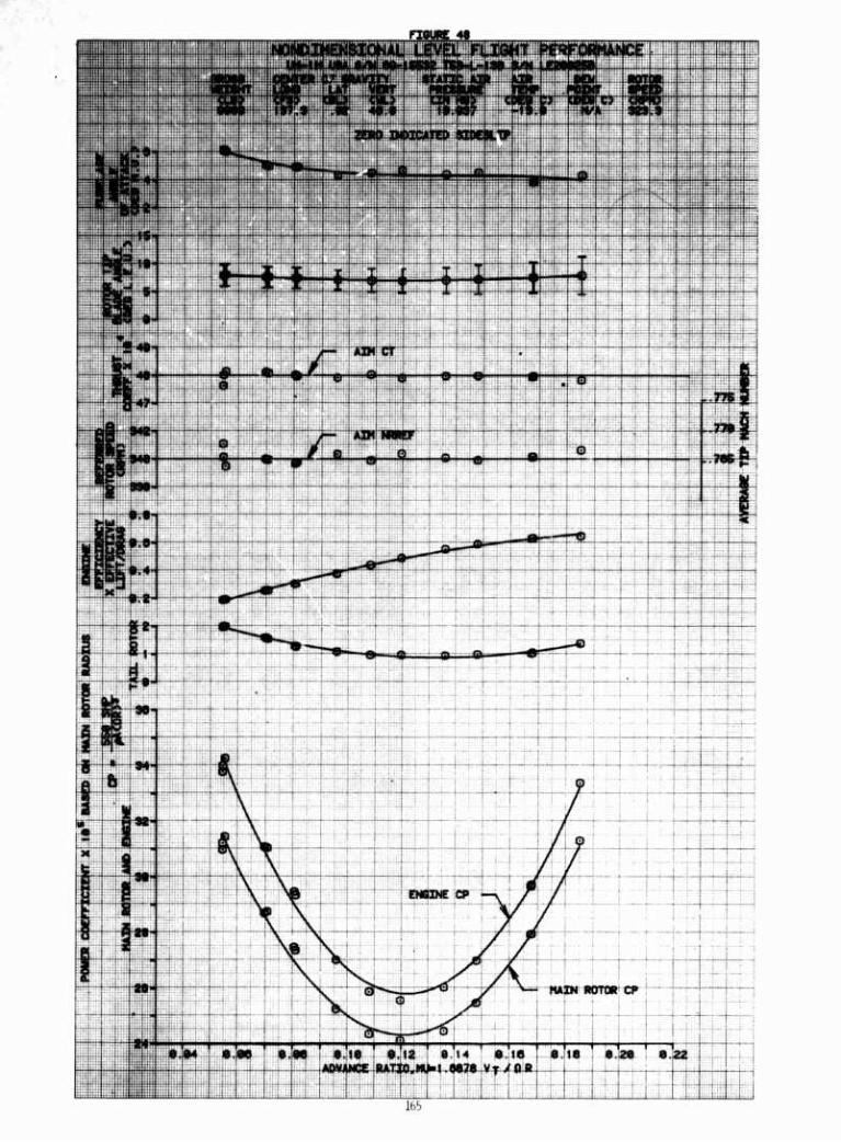
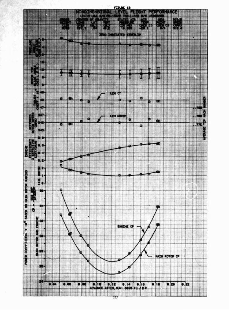
6. Twenty flights were conducted to obtain limited hover perfor- mance data and high thrust coefficient level flight performance data. Level flight data were obtained at thrust coefficients from 0.0040 to 0.0032 and referred rotor speeds from 300 to 350 rpm. These referred rotor speeds correspond to average tip Mach numbers of 0.675 to 0.788. Level flight performance tests covered: gross weight from 7020 to 9875 lb, rotor speed from 294 to 324 rpm, pressure altitude from 5520 to 14,840 feet, ambient temperature from-30.1 to+21.3 degrees Celsius, and airspeed from 20 knots (minimum usable Indicated airspeed) to limit airspeed (120 knots or less depending on weight and density altitude). Performance tests were conducted at a mid eg, at zero Indicated sideslip. In the clean configuration.
TEST METHODOLOGY
7. The overall adequacy of the FMC was determined by qualitative pilot communts, measured accuracy of the system am4 an evaluation of the range and scope of system capabilities. The pilots evalu- ated the Instructions, time required and ease of planning for each mission flight. Note was also made when Information was not available and the flight manual or another source was required. During flight the ease of use, flexibility to update Information and physical suitability of the hardware were evaluated. Accuracy was determined by the ability to validate the results of the BHT evaluation (ref 6, app A), comparison of predicted values with flight measurements, and comparison of normal and optimum mission profiles. The FMC functions and data available were evaluated with respect to operational needs. The calculator program was evaluated during 14 flights to three destinations which simulated typical utility missions as closely as practical. The flights were flown by an operational pilot (not a test pilot) solely by reference to standard flight instruments installed in the air- craft. Normal flight profiles were planned using the FMC as well as the operator*i manual. Optimum profiles were planned using the Prototype Optimum Cruise Charts and supplemental notes shown in appendix E.
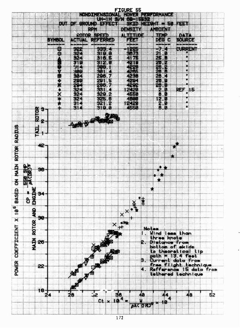
8. Blade stall a"d compressibility dita were obtained during level flight and hover test to complete the performance charac- terization for the fuel conservation effort. The referred rotor speed method was used for the level flight tests and the free flight method was used for the hover tests. All data were obtained at stable conditions in a nonturbulent atmosphere. Hover tests were flown only when winds were less than 3 knots. Data were recorded on magnetic tape in pulse code modulated (PCM). Test techniques and data analysis methods for the data in this report are described in detail in appendix D.
RESULTS AND DISCUSSION
GENERAL
9. The FMC was evaluated for flight planning and In-flight use during fourteen mission flights and calculator generated data were compared to engineering source data (ref 15). The FMC had many good features such as a very comprehensive set of limit checks. The calculator program accurately reproduced the source data. The HP-41CV calculator has significant advantages of cost, size, and availability over other electronic computing devices. The FMC's major faults were lack of an Integrated flight planning mode and relatively slow execution, resulting In longer planning time using the program than using the operator's manual. Operation and instructions need simplification for operational use. To achieve a one percent accuracy may require some form of "regressive modeling" where the program is updated with current data for the individual aircraft. To improve the speed and operating complexity and add other desired features may require a more sophisticated calculator than the HP-41CV.
10. Fourteen round-trip flights were made to determine the actual fuel savings using optimum flight profiles and to evaluate the calculator and program under operational conditions. The FMC did not provide optimum airspeed or rotor speed and Its optimum altitude was in error, so prototype operators manual optimum cruise charts were used to determine optimum flight profiles. Fuel savings were determined by comparing fuel use on flights using normal and optimum flight profiles. Overall fuel savings were 19% using optimum profiles compared to normal profiles. Fuel loading variation caused actual range or endurance uncertain- ties approaching 19%. Twenty performance test flights were conducted to provide a level flight data base in the high thrust coefficient range and to expand the hover data Mach number range. These data can be used to characterize blade stall and compres- sibility effects.
CALCULATOR EVALUATIOI'
11. The FMC was evaluated primarily for enroute performance (cruise, climb and descent) during the mission flights. Additional information used for this evaluation included: (1) use of the calculator by a variety of pilots on other ml:slons, (2) the field trials of reference 6, (3) other services performance calculators, (4) commercial aircraft performance calculators and onboard flight management computers, (5) Army operator's manuals mission planning requirements (ref 16), (6) an AEFA in-house optimum cruise demonstration program, and (7) an earlier onboard hover performance computer (lift margin system) evaluation
(ref 17). The FMC was oriented towards the field evaluation rather than towards an operational production design. This was done to permit evaluatlcn of a variety of possible features and functions. For example, several Input and output formats were used to allow selection of the most desirable formats. A produc- tion design for operational use should have a single Input format and a minimum of output formats. Several functions were late additions and not fully developed. These Included: weight and balance computations, more comprehensive limit checks, and engine performance variation capability. Comments and recommendations are generally oriented towards production version development of the FMC program for operational use In the UH-1H. However, some comments are applicable to other systems as well.
12. The HP-41CV calculator has been used for many performance applications. These programs generally duplicate the performance presented In the operator's manuals by using mathematical fits to existing data. This approach has two advantages. The programs can be produced by programming services with little or no knowl- edge of the Individual aircraft thereby reducing program develop- ment time and costs. It also simplifies data verification so the program can be introduced operationally and used in place of the operator's manual data in minimum time. An alternative approach is physical analog modeling. The FMC program was a combination of copying operator's manual data and analog modeling of basic test data.
13. The FMC program allows temperature variation but limits minimum cruise speed to 85 knots (except maximum endurance) and climbs to maximum rate of climb airspeed and power. Only limit airspeed is provided for "best cruise speed". The FMC optimum altitude function is easy to use but it does not include wind effects, optimum airspeeds or rotor speed. A simple correction to specification maximum power is provided. An operational program should provide optimum power, rotor speed, airspeed and altitude fur optimum climb, cruise and descent over the full range of weights and temperatures. The calculator provides easily read digital data at specific conditions.
14. Performance data accuracy is dependent on "specification" engine performance. Test experience (ref 3) indicates that fuel flow variation between engines or over the life cycle of an engine model is small (« 57,), However, maximum power available variation is large. Test engine power available of the T53-L-13 varied 15 percent from the reference 15 tests tc the reference 3 tests. The FMC incorporated a correction allowing a torque increment (relative to specification power available) input. This delta torque increment comes from the Turbine Engine Analysis Check
(TEAC) data, a maintenance procedure performed on newly installed engines. This value is accurate only at the TEAC conditions and will vary with time and engine condition. A previous method that provided better data was to determine power available from the applicable gas producer speed (Nl) and measured gas tempera- ture (EGT) relations to power and their limits (ref 17). These relationships are currently included as the "power assurance" function in FMC, however they are fixed at reference 15 test engine values. They could be established for an individual engine based on the initial TEAC and Health Indicator Test (HIT) baseline data and updated using the daily idle and HIT check data. This method has the advantage of not requiring a maximum power check and should substantially improve the prediction accuracy for power available dependent performance. Some method of updating power available with service time and engine condition should be incorporated.
Pilot Comments
15. Pilots generally responded favorably to the use of a calcula- tor as a better method to obtain performance information. The calculator was much easier to use in flight than the operator's manual. It was determined that the calculator could be read with much greater "precision" with greater ease than the graphical operator's manual data. The requirements for preparation of operator's manual data require that the data scaling be such that it can be read to one percent precision (two percent incre- ments) and at least as good as cockpit indicators. Some operator's manuals do not meet these requirements. Under poor conditions (in the aircraft with vibration, turbulence or darkness) this readability decreases. The output precision of the calculator can be misleading by Implying much greater accuracy than actually exists.
16. Two factors reduced the acceptance of the calculator; function execution time and the tendency of user induced inadvertent stoppage. A major potential benefit of the calculator is to reduce the time and effort for administrative planning of a flight. Some FMC functions required times exceeding two minutes which prevented a reduction of planning time over use of the operator's manual. Except for the longest (Yuma) mission flights, prefllght administration and planning time exceeded the flight time. Calculator/computer assistance in completing the various forms including performance planning, weight and balance and others could significantly reduce this administrative burden. The contractor indicated that search and execution time would be improved when the program was written on a production "PROM" chip. An execution time of five seconds. Independent of laput
tine would be an acceptable goal. This nay require a calculator nore advanced than the HP-41.
17. The long er.ecution tine sometimes caused the user to inadvert- ently stop the progran prior to conpletion because of apparent inactivity. The "input" key is actually a "run/stop" key so that pushing it while the progran is running will stop the pro- gran. The FMC progran showed a variety of displays while programs were executing. These did not provide the user with a program status and led to confusion as to whether or not the calculation was proceeding. This fault is inherent with the programmable calculator and can only be nininized and explained clearly in the operating instructions. A nore serious difficulty encountered by most users was unknowingly switching fron PDQ to basic calcu- lator node. The inclusion of this sinple calculator node was a serious detriment to the acceptance of the evaluation program. A production version using a programmable read only memory (PROM) chip would avoid this and allow the full calculator capability Independent of the performance progran. Pilot opinion of the value of the FMC covered the whole spectrun from "no conceivable value" to "an immediate necessity long overdue". The predominant opinion was that it had significant potential value but required substantial refinement with the planning node capability the most needed modification i.e., "1 want it to print ny Perfornance Planning Card (PPC)."
Documentation
18. The users manual was poor because of apparent large volume including much infornation extraneous to operation and detracted from user acceptance. The single document (ref 18) contained overall project information, background infornation, field trail plan and methods, as well as operating instructions. The size was similar to the aircraft operator's manual and was printed on one side of the paper in fairly large print. Ultimately the calculator operating instructions should be integrated into the pertinent sections of the aircraft operator's manuals i.e., limits, weight and balance, performance, normal and emergency procedures. "Help files" as used on computers should be con- sidered if substantial memory expansion is included or more capable calculators are used. This would require the use of a printer or auxiliary display. Other factors that need improvement include complete abbreviation definitions and, where applicable, use of established standard abbreviations. The detailed program descriptions should be supplied in a separate document.
•
Phyical Characteristics
19« The HP-41CV calculator Is one of the most capable calculators available that Is truly pocket sized. Its overall dimensions are 5.6 X 3.1 X 1.3 Inches. This size and the light weight of 8 ounces make It very portable. It Is easy to mount on the standard kneeboard and still leaves room for notes. However, the small face that Includes the display and 39 keys requires small keys closely spaced. This characteristic Increases the prob- ability of erroneous key entries. The tactile "click" provides a distinct feel when a key has been activated. However, while wearing gloves in flight in a vibration or turbulent environment correct key entry is difficult. With moderate or worse vibration, the calculator and key entry hand must be isolated from aircraft vibration by raising them from kneeboard. Using a pencil eraser helps proper entry. A "touch pad" overlay that locks over the keyboard is available, that Increases the area, separates the keys and increases the pressure required to activate the key from approximately 5 to 16 ounces. Its major drawback is that it masks the tactile click, particularly with gloves. Pilots must be cautioned (as they were in ref 18) to visually check the numerical value prior to data input.
20. Another inherent limitation of the HP-A1CV is the display. The built-in display consists of 12 alpha or numeric characters scrol- lable to a maximum of 24. The scroll rate is two per second so a full message would take 6 seconds to display. The characters are generated from a 14 segment liquid crystal display (LCD) so the number and legibility of the characters are limited. For example a question mark (?) should not be put next to numeric values because of its similarity to a seven (7); even experienced users will misinterpret the two characters. This limitation can be overcome with auxiliary electronic displays or printers where a 7 X 9 dot matrix is used for character generation. This permits use of 128 standard characters or even design of special charac- ters for the program. If the HP-41CV is used for future perfor- mance calculators, an auxiliary lighted display should be con- sidered. Neither the display nor the keyboard has integral lighting. BHT designed a modification to the standard pilots knee board to provide calculator lighting for the reference 6 field trials. This lighting method was not evaluated.
Accuracy
21. Calculator introduced errors will be insignificant bocause the ten place calculation precision is far more accurate than other error sources. The high output precision available from the program misled most pilots about the overall accuracy. For
10
example, altitudes were output to the nearest foot and weights to the nearest pound. Consideration should be given to reducing the output precision. The reference 19 program rounded the cruise altitude to the appropriate 500 foot altitude Increment. The reference 17 computer rounded altitudes to 100 feet and weights to 10 lb. The most direct solution to this problem Is to output estimated error bounds as well as most probable value for each parameter. This would require a detailed error analysis and a substantially more sophisticated program. Estimated accuracy for each major parameter should be stated to the degree practical In the calculator operator's manual. This will define and minimize the margins required for performance data uncertainty to Insure safe operation.
22. Reference 6 Includes demonstrations of the calculator programs ability to reproduce the source data accurately. In some cases the source data are Inappropriate. For example, reference 15 engine data were used for the relationships of gas producer speed and exhaust gas temperature to power. Current operational engines are significantly different from these preproductlon engines of 20 years ago. However, if some method were Included In the program to correct the general relationships to current individual engine characteristics, accuracy could be improved. Another more signifi- cant example that determines UH-1H performance capability is directional control limits. The FMC used reference 15 data to determine the "10%" directional control margin. This data did not consider the variables of skid height, wind azimuth, rotor speed, control rigging or complete maneuver capability. Data published In reference 11 are considerably more accurate and include wind azimuth and wind speed at the most adverse rigging. The difference between the current (ref 11) data and the obsolete (ref 15) data could result in inadequate control at 14 knots lees wind speed or 2000 lb less gross weight than predicted by the FMC. Reference 11 data should be corrected for the rotor speed error (para 62) and used in future calculator programs and UH-UI operator's manuals.
23. An overall calculator accuracy of one percent is desirable. This level of accuracy is usually adequate to allow proper decisions to be made. For example, one percent of the 9500 lb maximum gross weight, 95 lb, permits the proper decision on number of troops to be carried. One percent of 1A00 pounds of fuel, 14 lb, corresponds to less than 10 percent of reserve fuel and less than two minutes flight time at the worst condi- tions. Because of engine, aircraft and indicator systems vari- ability, some form of "regressive modeling" where the program Is updated with current individual aircraft data, will be required to achieve this level of accuracy.
11
Units - Conversions
24. The calculator program parameters were generally in customary U.S. aviation units (feet, pounds, knots, etc.), except for those peculiar to the Uh-IH, such as torque pressure In pounds per square Inch (PS1). These units are proper and desirable. One undesirable factor for the HP-'JICV 12-character display was the Inclusion of the units In the output display. This used up valuable display characters that could have been used to minimize nonstandard parameter abbreviations and to Include other enhance- ments. One exception to this Is temperature units, where degrees Celsius and degrees Fahrenheit are used with nearly equal fre- quency. If an expanded auxiliary display or a different calcu- lator with expanded display is used, units could be included. The calculator piogram had several units and parameter conversions including: degrees F to degrees C, indicated to pressure altitude, and indicated to true airspeed. The indicated to pressure alti- tude conversion was backwards. If a pressure higher than 29.92 in.Hg. (standard) was input, the calculated pressure altitude was higher than indicated, not lower as it should be. The mechanics of the conversions were rather cumbersome. They could be mechanized such that a single keystroke could convert from a nonstandard unit to the standard unit and the secondary (gold) key plus the conversion key would convert from standard back to the nonstandard unit. Unless substantially more memory is used or a more powerful calculator is used for future programs, unit conversions should be of secondary or lower consideration to the primary performance function requirements. If computing capability is increased, other conversions that should be considered are: fuel weight to volume (gallons) and density and metric conversions for use in the European environment.
Data Ranges
25. Data ranges should not be arbitrarily limited, such as the minimum cruise speed which was limited to 85 knots. Performance computation capability should be available for any conditions at which the aircraft can operate. With performance computation capability available for all conditions, only the limits table (following paragraph) would have to be updated for limit changes. Performance Information Is most important at extreme conditions because flight will be more critical and the pilot will have little or no experience there and must rely on the calculated performance information.
Data Limits
26. Limit checks are where the program halts or changes execution when input or output values exceed aircraft operating limi :s or
12
reflect Impossible conditions. Limit checks serve three purposes. They prevent the pilot from inadvertently planning operations beyond approved limits. They allow the pilot to know and plan operations at limits to obtain maximum performance. Limit checks also reduce the possibility of erroneous data entry. The FMC program has a fairly comprehensive list of limit checks. In general, they are appropriate and have proper values. Their mechanization la quite cumberpome and could be improved substan- tially. When encountering or exceeding most limits, the FMC will not continue and the user must restart the performance calculation and input all previous valid data. A better method would be to leave the user at the input parameter that caused the limit to be exceeded. The limit value would become the new default value for that parameter so it could be used ir the pilot wished to operate at the limit. This would provide an easy way for the pilot to determine limits without knowing them ahead of time or using a separate procedure to determine them. Limits should fall into two categories; those under pilot control, such as maximum gross weight, airspeed, torque; and those beyond pilot control, such as minimum aircraft weight, maximum ambient temperature or maximum power. Those limits under pilot control should be exceedable on a second try, to determine what the performance would be in an emergency situation wnere limit observance is secondary and to determine what the next limit is and its proximity to the lowest limit. For example, hover per- formance is most likely to be limited by directional control. However, if winds are not a factor the pilot might want to know his torque-limited or maximum weight-limited performance. He may also wish to know the maximum power-limited performance and Its proximity to the torque limit to judge the likelihood of topping the engine if ambient temperature is difffrent than estimated. Additionally the parameter that determines the limit should be Indicated so the pilot will know which to monitor.
Input
27. Several levels of input should be preselect able. The lowest and default level should require input of the minimum number of parameters to obtain reasonably accurate performance. A higher level could include secondary parameters such as barometric pressure or humidity to improve accuracy at critical conditions. The most sophisticated input level could allow the user to pre-set the input parameter list or sequence for his calculator. The capability of the user to select, terminate or omit a calculation on the basis of an input value is a generally good concept. This was used for several of the FMC functions. Examples are the termination of cargo load items in the weight and balance function
13
by the input of zero weight and the deletion of the wind calcu- lations with the input of zero wind speed. While this approach requires additional knowledge of the user to know the input value codes, it provides a convenient and efficient means of tailoring input for a given performance calculation. A single input format should be used. The following format is considered a good compromise:
(parameter name) ?= (default value) no units
With the exception of temperature, there is no ambiguity of customary aviation parameter units within the Army. They need not be used in the actual display, since they use spaces that could otherwise be used for for better parameter name definition. For the HP-41CV, more than 12 characters are undesirable since this requires scrolling the display which obscures the initial parameter name characters. While the question mark more logically belongs after the equal slgr, it can easily be confused with a seven on the standard calculator display. A more sophisticated auxiliary display or calculator would allow a superimposed question mark and equal sign.
Output
28. Generally, the same condlderations for input apply to output. A wide variety of approaches have been used for output presenta- tion In existing and past performance data presentations. Enroute performance (cruise, climb and descent) can be limiteci to a moderate number of output parameters. The FMC has a primary cruise function as well as a maximum range, endurance and climb functions. Limit airspeed and optimum altitude were also provided as separate functions. Output from the cruise function includes: limit airspeed, fuel flow, required and available torque, ground speed, reserve fuel, enroute time and fuel used. Vte maximum range function is similar except that total fuel is li{i:.t and distance to reserve fuel is output. Maximum climb and a. ourance output is time and distance. These functions can only bt used at minimum power airspeed and, in the case of climb, at maximum power available. Most FMC functions provide a "manual" mode that stops at every output parameter or an "automatic" mode that pauses at intermediate output and stops at the final output. Each primary enroute function takes approximately two minutes to execute.
29. The FMC program has four hover functions: gross weight, torque, endurance, and time. Each of these functions output some combination of the following parameters: maximum hover weight and lift margin at both maximum power and for ten percent
14
i
directional control margin, maximum skid height capability, power required to hover, power available, vertical climb rate, fuel flow, hover time with remaining fuel and fuel for a given time. The operator's manual graphical data provide these parameters and In addition allow the performance problem to be worked back- wards so that limiting Input parameters can be directly deter- mined. For example, for a given hover load or gross weight, maximum altitude or ambient temperature to hover can be deter- mined. Similarly at given conditions the maximum wind velocity to maintain ten percent directional control margin can be deter- mined. This capability should be available from the calculator program.
30. The FMC uses an even greater variety of formats for output than for Input. Particularly troublesome to all users was the format with the parameter name(8) appearing on the display for only one or two seconds prior to the value(s) line. This required the user to continuously watch the calculator for up to two minutes so that he would not miss the label and end up with undefined numbers In the display. Some abbreviations and terms were not clear (such as SK HT:PDM) and In some cases disagreed with Army definitions (such as BOW: basic operating weight). The format recommended for Input Is also recommended for output, however, there may be some specific cases where an alternate output format Is better. The concept of user selectable levels of parameters Is also applicable to output. The lowest level (default) would require the minimum Input and output to complete the performance planning card (PPC). The next level would add those parameter« necessary to Improve accuracy and provide additional output information for those missions where performance Is known to be critical. The highest level would allow the user to pre-select parameters In the desired sequence. This would allow termination of the output sequence for any performance function after obtaining Information required for a particular mission. This sophistication may be beyond the capability of the HP-41CV calculator.
Specific Performance Comments
31. The following paragraphs discuss specific functional areas of the FMC and performance areas not In the program.
Weight and Balance:
32. The FMC weight and balance function Is logically organized, requires minimum Input and provides mo it needed output quickly. However, It was added late In the development and was not fully developed. Several Improvements are needed. The Interaction
15
with other functions, providing gross weight and load information, was a good feature, but not allowing fuel weight input within the function was objectionable. Weight and balance is usually the first step in planning so all required input should be within the function. For missions not requiring a weight and balance computation direct input of gross weight, load, fuel weight and possibly eg data to the main program should be retained, default values should be provided for all inputs. Limit checks against eg limits and precautionary areas must be provided, possibly with instructions for revised loading if limits are exceeded. The limit checks had the same fault as other functions in that input errors or exceeding limits required the user to start the function over. The program should return to the input that exceeded the limit, with the limiting value provided as default and all previous valid input retained. The type of aircraft fuel system input should be removed from the calculator program if all UH-1 aircraft have been converted to crashworthy systems. The fuel computations should include provisions for the standard internal auxiliary fuel tanks. They could be automatically invoked if fuel load is greater than normal capacity. One possible additional dedicated input is the cargo hook load. In addition to the total moment, eg and gross weight, the function should provide any other Information required on the weight and balance form. A related feature not part of the weight and balance function was the capability to operate in either of two modes, aircraft gross weight or load weight. The two modes allowed the user to work with gross weight or Just cargo, equipment, and passenger load, whichever is most convenient. While conceptually good, this feature required additional knowledge and confused some users.
Ground/Taxi Operations:
33. There are no provisions for ground operations, specifically engine start and idle fuel use. Engine idle fuel flow is approxi- mately half of normal cruise fuel flow and two thirds of optimum cruise fuel flow. Hov>>r/air taxi fuel flow le greater than cruise fuel flow. Therefore, ground engine operation will have a significant effect on overall range and endurance and must be considered to plan missions accurately. The default 3 foot skid height, within the hover time function, could be used for air taxi. Ground/taxi fuel use calculations could be mechanized to input a single fuel used value based on experience or previous calculations. Inputlng zero ground fuel would then invoke the detailed calculations for ground idle time, flight idle time and hover/taxi time prior to takeoff and output and adjust Initial fuel for total ground fuel used. For multi-engine helicopters this becomes even more complex since single engine, dual engine and auxiliary power unit (API!) time must be considered.
16
Engine Performance:
34. The FMC has a "power assurance" function that provides gas producer speed (Nl) and exhaufL gas temperature (EGT) for a given Input power (torque and the assumed fixed rotor speed). The relationships used are obsolete and In error. However, even with current data and proper characterization, Input of measured Individual engine baseline data will probably be required to achieve useful accuracy. In addition to Nl and EGT, fuel flow as a function of power (torque and rotor speed) should be Included so that It can be determined Independent of any partlcula: per- formance phase or maneuver.
Hover:
35. The four FMC hover functions (gross weight, torque, time and endurance) could be combined Into two or possibly a single func- tion. Maximum performance values could be returned for the default values at the Input request. The hover weight Input request could have a default value equal to the maximum hover weight and the hover time Input request could have a default value equal to the total time available with remaining fuel. The hover gross weight function outputs power-limited and directlonal-control-liralted maximum gross weights. A better method would be to provide maximum wind velocity for adequate pedal margin at the selected hover gross weight and conditions using current operator's manual data (ref 11, app A). Alter- natively, the maximum weight for adequate pedal margin could be output for a given wlndspeed Input. In a planning mode, fuel used for an Input hover time should be subtracted from fuel remaining prior to takeoff.
Takeoff:
36. The FMC program does not provide takeoff performance data. Takeoff performance data (distance required to clear a 50 foot obstacle) Is useful for tactical helicopter operations at calm wind and level surface conditions. The calculator could allow more complex data than can be provided In the operator's manual. For example. It could calculate the maximum safe load that can be flown as winds and temperature vary from a given area where obstacle height and distance are known. The tradeoffs between an uphill or downwind takeoff under conditions where one or the other Is required could also be calculated. Recent operator's manual takeoff data have been presented with most independent parameters in terms of maximum ICE hovering skid height. There- fore, takeoff performance could be added to the hover performance function since IGE height is already computed when out-of-ground effect (OGE) hover is not possible.
17
Climb - Descent:
37. Except for the vertical climb output from hover the only climb and descent performance available from the FMC is maximum perfor- mance climb at maximum power and best rate of climb airspeed. This performance, based on specification power available, is not practical since flying qualities are poor at the airspeed and maximum power (topping) is difficult to maintain accurately. The time, fuel and distance traveled during climb or descent at any airspeed and power must be accounted for to accurately plan range or endurance.
Winds and Temperature:
38. The FMC has two levels of wind input. If zero windspeed is input, all calculations are made with groundspeed equal to true airspeed and no further wind input is requested. If wind speed is not zero, wind direction and course are requested and ground- speed is corrected for winds. The corrections are made as though course is actually heading and are in error. For example, a 90 degree cross wind to the course results in no difference between groundspeed and true airspeed calculations. With a 90 degree crosswind, groundspeed will be less than true airspeed because of the crab angle required. Determination of true optimum cruise altitudes requires input of wind variation with altitude and flight path.
39. The FMC calculated temperature at altitude (assuming standard adiabatic lapse rate of -2 degrees C per thousand feet) from an input temperature and altitude. Temperature observations during the mission tests showed this method using surface temper- ature and altitude would result in temperature under estimated by as much as I30C at cruise altitude. This temperature difference would result in a 2% error in planned range or fuel use at a given altitude. It could cause errors in determining optimum altitude of as much as 4000 feet which would cause up to 67. error in planned range or fuel use. This temperature error could also result in optomlstlc planned maximum hover capability of as much as 1100 lb. Performance can be recalculated in-flight with actual temperature Input to correct planned performance.
Emergency Performance:
A0. The FMC provides no emergency performance information. The most significant emergency performance information for the single engine UH-1H are the airspeeds and rotor speeds for minimum rate of descent and best glide in autorotation. Height - velocity Information would also be useful for planning. For multi-engine
18
helicopters there is a multitude of additional Information required for one engine out performance.
Future Development
41. Future performance calculators must Include a planning mode that runs more or less automatically requiring minimum special knowledge and Input from the user. The planning mode should do all necessary calculations between flight phases and provide output or print any required forms. For Inflight use, five seconds from last Input to the desired output Is an acceptable time. Regressive modeling In which current Individual aircraft data Is used to update the program may be necessary to ach., /e acceptable accuracy under operational conditions. Automatic data Input from aircraft sensors would make available updated performance data. Such a system using the HP-41CV system with available peripherals Is technically feasible. For the UH-1H, airspeed (dynamic pressure) and air temperature, preferably compressor Inlet temperature, would bu required. For modern aircraft all necessary signals may be available on a data buss. A display would also «ignlficantly enhance the in-flight benefits of the performance calculator. This combined with the automatic data input feature of the HP-41CV could provide continuous data presentation. The changes recommended in this report would tax the capability of the current HP-41CV calculator. There are more advanced calculators availible that should be considered. Inte- gration of performance data into current and future aircraft that have general purpose computers and displays could have additional safety and mission enhancement benefits.
42. The portable calculator provides a means to determine both planning and in-flight performance data and the potential to both improve the data and reduce the effort. The use of fixed base computers could improve planning capability and complement the portable calculator's capabilities. The ability to access other data bases could also significantly enhance flight planning. Reference 20 describes a system using a small personal sized computer to integrate performance and weather data. Additional integration should include accessing local data bases for aircraft configuration, condition, baseline performance data, navigation and possibly tactical data. For a portable calculator such as the HP-41CV, the ground based computer could load the planning data and other precomputed data such as optimum cruise profiles which are beyond the computing capability of the calculator. For aircraft where a performance computer is installed, such data would be transferred by some data storage medium. In-flight data different from the planned data would alert the pilot to changed conditions, malfunctions and other reasons to reconsider
19
the planned data. Electronic data storage and performance computing capability, from portable calculators through onboard computers to fixed base computers, can enhance the productivity, efficiency, utility and safety of helicopter flight»
■
MISSION FLIGHTS
General
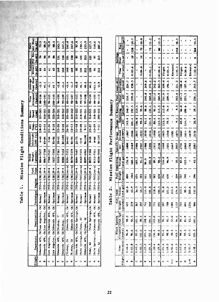
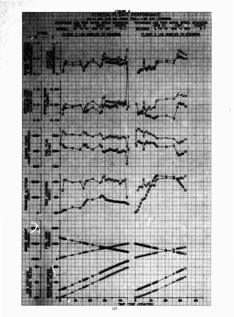
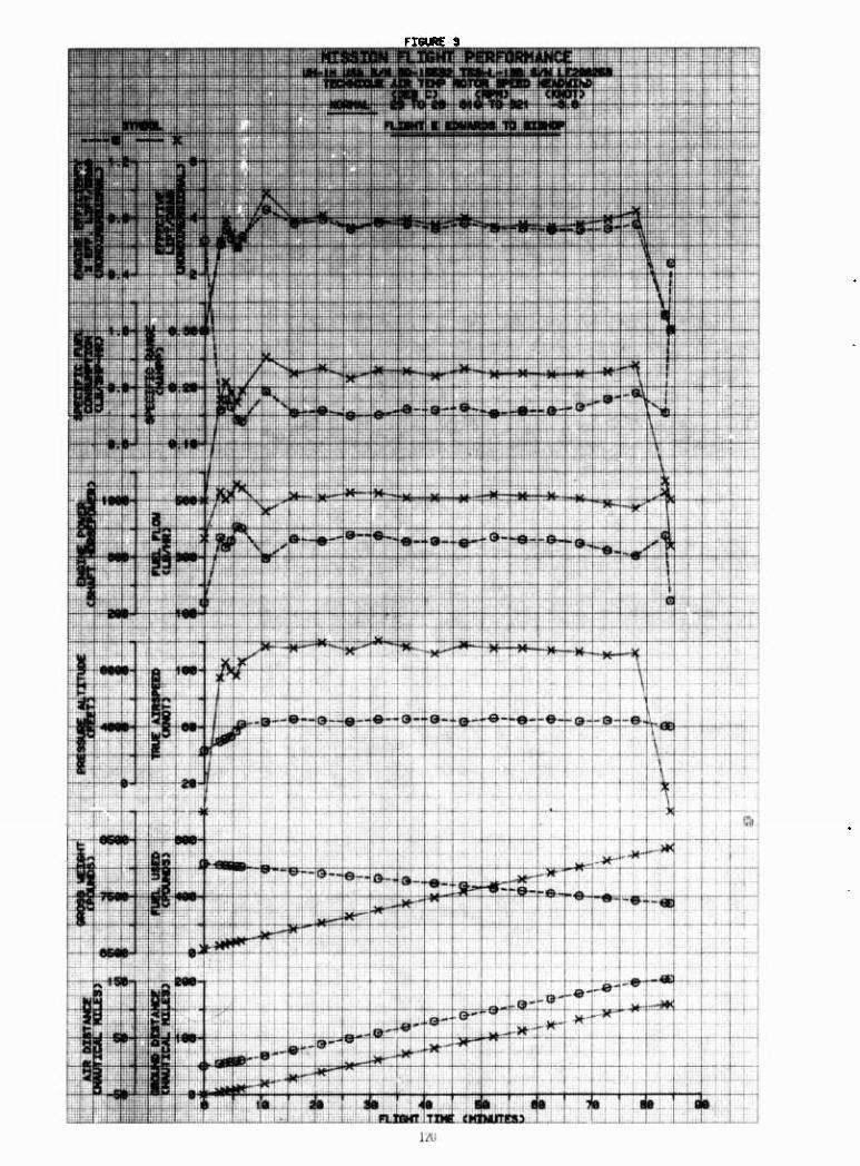
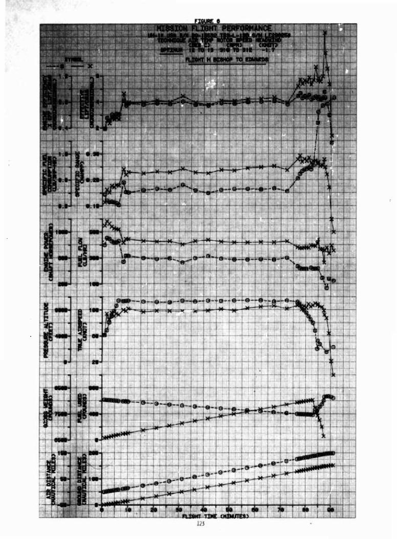
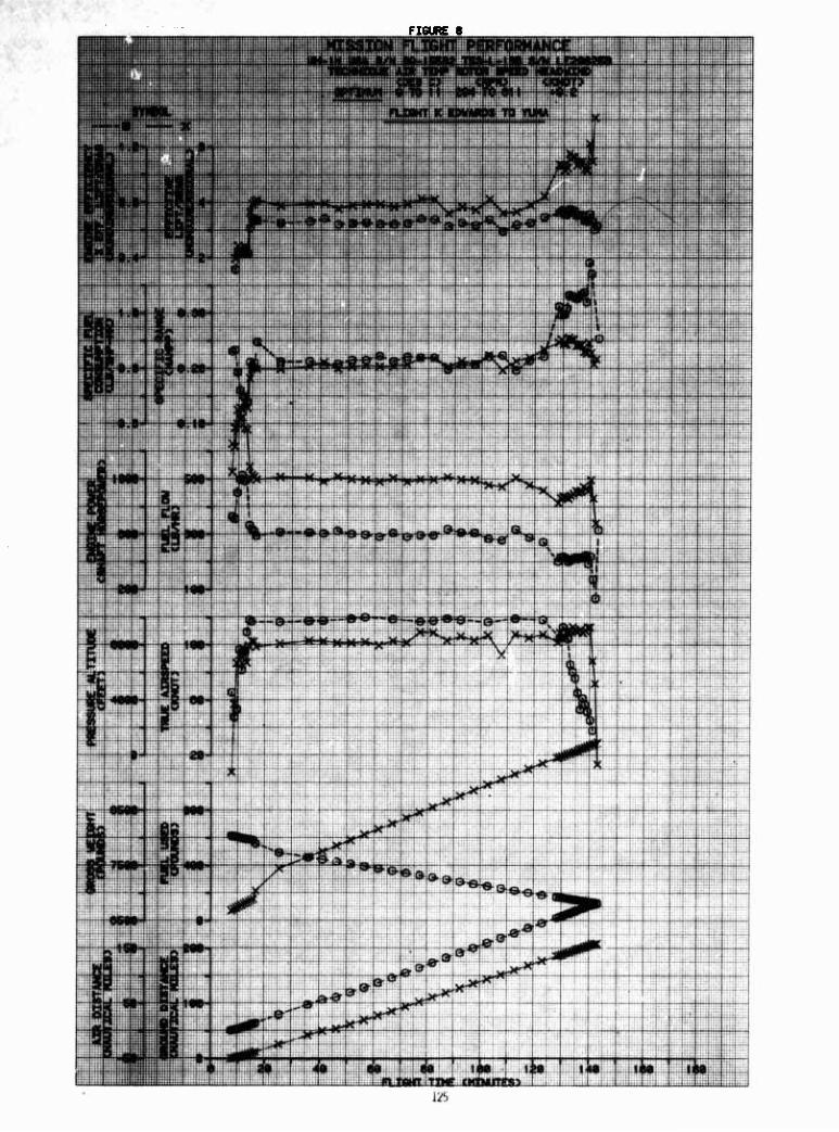
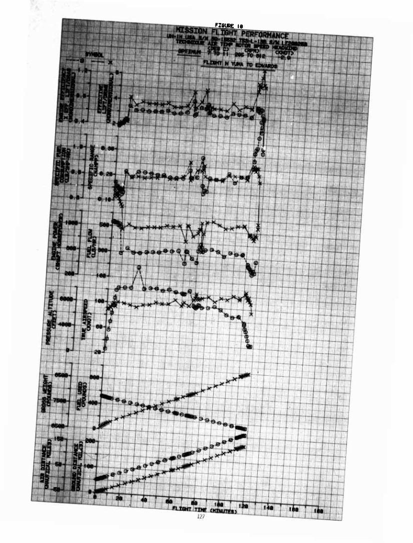
43. Fourteen mission test flights were made from Edwards AFB, California to three destinations: Los Angeles International airport, Los Angeles, California; Bishop airport. Bishop, California; and Laguna Army Airfield, Yuma Proving Ground, Arizona. The "normal profile" flights to and from Yuma required a fuel stop at Palm Springs, California. Two mission flights were flovn to and from each destination. Flight routes were planned using the most direct route considering airspace restric- tions and terrain suitable for forced landing following engine failure at cruise altitude. One leg of each round trip was flown using "Normal" flight profiles and the other using "Optimum" flight profiles. An approximation of fuel savings was made by comparing results from "Normal" and "Optimum" flight profiles. Time history data for the mission flights are shown In figures 1 through 10, appendix F. These flights covered a spectrum of UH-IH range capability, air traffic control constraints, weather conditions, and other operational variables. Mlsnlon test flights were designed to simulate operational missions as closely as practical. The flights were flown by operational pilots (not test pilots). Three different flight crews were used. The engine models used were the T53-L-13B and the T53-L-703.
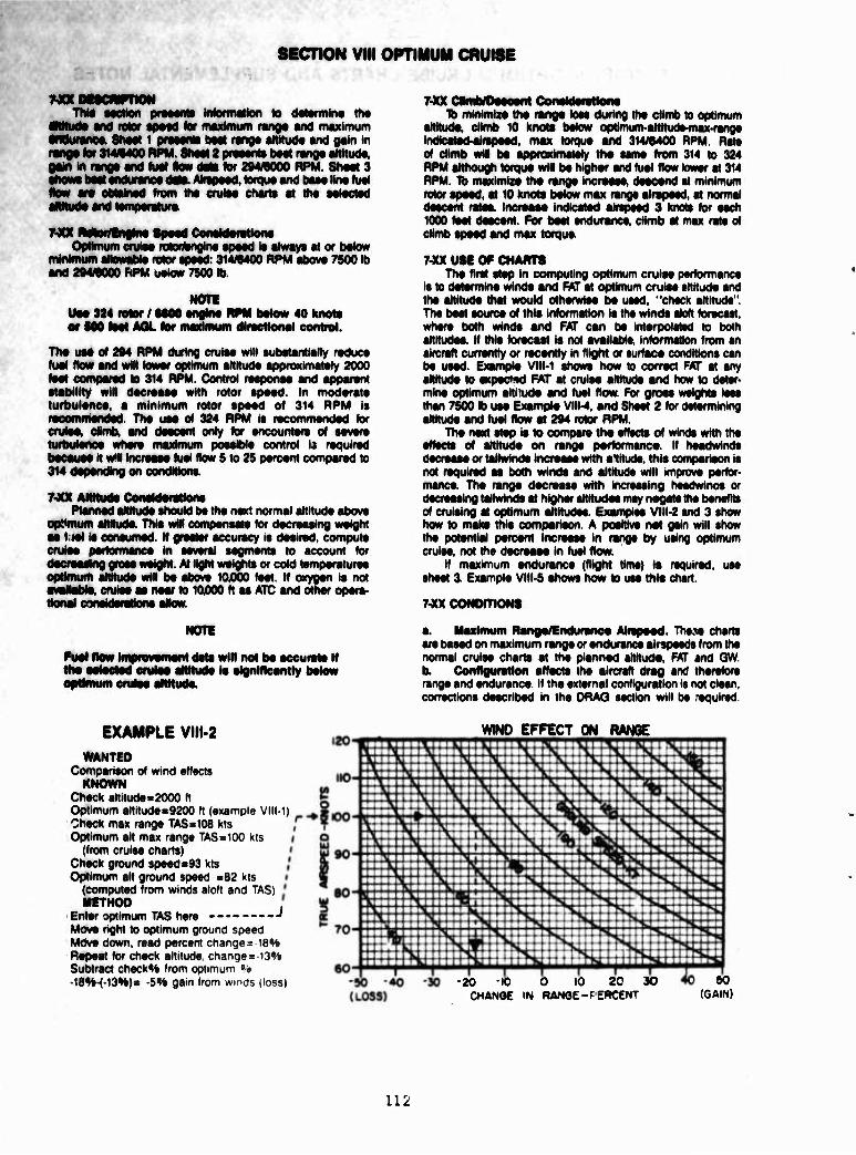
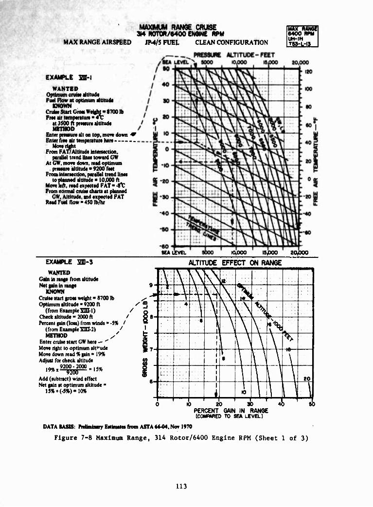
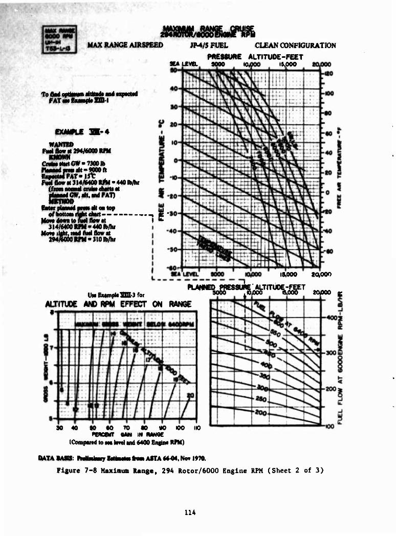
44. Normal flight profiles were In accordance with the UH-IH Aircrew Training Manual (ATM), reference 21, appendix A, ind current training procedures. Optimum flight profiles were deter- mined from the Prototype Optimum Cruise Charts and supplemental notes extracted from reference 2, Included as appendix E. The major difference between the two profiles was the rotor speed and altitude used during cruise flight. The normal flight profile used maximum rotor speed (defined as normal) and the optimum flight profiles used minimum rotor speed. Normal flight profile altitude was established relative to terrain and optimum altitude was that which gave maximum specific range for the conditions.
45. To the extent possible, missions were planned using the FMC. Planning aspects such as time, ease of operation and ac)uracy of the FMC were compared to normal planning using the operator's manual. Most of the minimum required (PPC) performance Information
20
such as hover performance and V^ was available from the FMC. Some of the performance Information such as directional control limits was substantially in error. It was intended to plan the mission flight profiles using the FMC and compare FMC predicted flight performance with actual performance measured by test instrumentation. However, because some Information was not available, optimum flight profiles could not be determined from the FMC. It contained no information on optimum rotor speed, airspeed, climb and descent power or airspeed schedules. The FMC optimum altitude was several thousand feet higher than appendix E optimum altitude and at the mission flight conditions always above 10,000 feet, the limit for continuous cruise without supplemental breathing oxygen. The FMC operating instructlc. i indicate that VJJE is "recommended cruise velocity". Vj^ is provided by the FMC. At the test conditions, maximum range, calm wind, cruise airspeed is at or slightly below Vj^. However, at temperatures below standard, maximum range airspeed is as much as 25 knots below Vfjj;. This difference has a large effect on range and fuel use. Additionally, maximum range airspeed decreases by approximately AOZ of the tall wind magnitude. The FMC predicts fuel used only during the cruise portion of the flight, and does not Include fuel used during idle, taxi, takeoff, climb or descent. This FMC data is compared to fuel use and maximum range mission test data in paragraph 64.
Flight Conditions
46. Flight conditions for the mission flights are summarized in table 1. The flights were conducted under Visual Flight Rules (VFR) to minimize route or time deviation requirements from Air Traffic Control (ATC) facilities. ATC conatcaints were mlnlnwl on the Bishop flights (E-H), requiring only VFR departure and arrival procedures from the Edwards complex. ATC constraints for the high traffic density Los Angeles flights (A-D) ware extensive. Flight E to Bishop encountered intermittent llj»ht rain and light to occasionally moderate turbulence. Flight H from Bishop was in similar weather, and slight route deviations were required to maintain VFR cloud separation requirements. Flights K through N were in light or occasionally moderate turbu- lence. Flight N required both route and altitude deviations to maintain cloud separation. For the other mission flights, the weather conditions were clear with no more than light turbulence.
47. With one exception, mission flight conditions were estab- lished and maintained by reference to standard uncalibrated production indicators. The sensitive test rotor speed indicator was used to limit minimum rotor speed to the true value. Use of the standard indicator with its systematic error would have
resulted In rotor speeds significantly be the minimum rotor speed limit. While the pilots uted the standard Instruments during flight, the flight conditions and performance shown in tables 1 and 2 were determined from test instrumentation using methods described in appendix D. The following paragraphs discuss each of the conditions in table 1»
Loading and Fuel Quantity:
48. Nominal loading was 8100 lb engine start gross weight which represents 1000 lb pay load, a crew of two and full fuel for an operationally-configured aircraft. A mid longitudinal eg (fuselage station (FS) 137) and a mid lateral eg were used. Precise fuel loaaxng was not attempted, since this was considered an operational variable. Therefore, engine start gross weight varied with the actual fuel loading from 8035 lb to 8162 lb. The test aircraft had 205.7 gallons (gal) usable capacity In a level attitude. The actual fuel volume capacity varies approxi- mately 5 gal per degree of lateral attitude with an Increase for left side low and a decrease with a rlgnt side low. Longitudinal attitude has no significant effect on capacity. Fuel capacity variation with aircraft lateral attitude should be considered when fueling for missions that require maximum range or endurance. This Information should be included in the operator's manual.
49. Fuel density also impacts maximum cruise capability and for the mission flights ranged from 6.34 lb/gal for flight L to 6.70 lb/gal for flights J and M. Jet fuel density variation with temperature is -0.00657 lb/gal/deg C. The combined volume and density variation resulted in mission fuel weights from 1087 lb on flight L t5 1233 lb on flight J, a 13 percent varia- tion. Precise planning should utilize the fuel quantity Indicator which reads out in lb of usable fuel remaining. This instruction should be included in the operator's manual.
50. Where the objective is minimum fuel consumption rather than maximum range or endurance, minimum fuel weight rather than maximum Is desired, ideally, the aircraft should land is the low fuel warring activates, with cooldown and shutdown accomplished on reserve fuel. At low altitude and cruise speeds from maximum endurance to maximum range, the weight of additional fuel burned per hour is approximately two percent of the excess weight. For example, if the aircraft lands after a one hour flight with 200 lb more fuel than required for reserve, an additional 4 lb fuel consumption would occur during the flight. This Increases to approximately three percent at optimum altitude. The excess weight fuel burn at speeds below best endurance speed increases to ten percent or more at hover or nap-of-the-earth speeds,
23
depending on weight and altitude. This applies to any excess weight caiiled on a flight, not Just fuel. A suitably developed performance calculator or onboard performance computer would mini- mize the margins required for aircraft performance uncertainty.
■
Cruise Conditions
51. Pressure altitude, ambient air temperature, rotor speed and true airspeed ranges for the cruise portion of each mission flight are summarized In table 1. Additionally, sideslip angle did not exceed six degrees for any recorded cruise condition. The latest operator's manual (ref 11, app A) does not contain any information on optimum cruise conditions (other than the normal calm wind "best" cruise speed.) The FMC optimum altitude was several thousand feet in error compared to reference 15 data. The calcu- lator contains no information on optimum airspeed, rotor speed, wind effects on optimum conditions or optimum climb and descent, power and airspeed schedules. Therefore optimum profiles were determined from appendix E data adjusted to normal VFR cruise altitudes and by AR 95-1 crew oxygen use rules. The test aircraft had oxygen but it is not normally available in UH-1H aircraft. Portable oxygen systems are available and Integral oxygen genera- tors using engine bleed air are under development (ref 22, app A). Except for very light weights or cold temperatures the majority of cruise altitude benefits can be achieved at 10,000 feet or less.
Cruise Altitude and Temperature:
52. Normal flight profile cruise altitudes were nominally 1500 feet above ground level (AGL) with pressure altitudes from -300 feet to 7500 feet, as terrain elevation varied. Optimum flight profile cruise altitudes varied from 7500 to 10,500 feet mean sea level (MSL), depending on weight, rotor speed and ambient temperature. Pressure altitudes were from 7800 to 10,500 feet. Ambient temperature at cruise altitude averaged approximately 15 degrees C above standard for the flight altitudes. The optimum rotor speed gains in cruise performance were minimal at these warm temperatures and cruise performance improvements will Increase at colder temperatures compared to these test results (see flg. B, ref 3).
Cruise Rotor Speed:
53. Normal cruise Indicated rotor/engine speed was 324/6600 rpm. This has since been reduced to 314/6400 by reference 11. On the first round trip to Los Angeles, rotor speed was inadvertently set using the test Indicator at the normal 324 rpm value for the
24
entire flight (flights A and D). The use of the pruductlon rotor/engine tachometer Indicator during other flights resulted In sctual rotor speeds of 318 to 323 rpm. While this error Improves cruise performance, It has other serious Implications discussed further In the Instrument accuracy section (para 62). For the optimum mission flights the rotor/engine speeds were minimum allowable: 314/6400 rpm above 7500 lb, and 294/6000 rpm below 7500 lb gross weight. The 304 rotor rpm limit below 8000 lb allowed by reference 14 for these tests was not used as It Is not proposed for an operational limit.
Cruise Airspeed:
54. The normal mission cruise airspeeds were selected by the pilot, on the basis of vibration and comfort. They were usually In the 90 to 100 knot Indicated airspeed range. This resulted in cruise true airspeeds from 85 to 120 knots with a variation of as much as 28 knots on a flight. Optimum cruise airspeeds were determined from reference 10 and modified per information in appendix E. They were usually above limit airspeed (V^E) and therefore limited to V(^. Optimum flight profile cruise true airspeeds varied from 92 to 110 knots. Optimum cruise speeds varied a maximum of 16 knots on a flight but generally varied less than 10 knots. Reference 23 indicates that cruise, climb and descent performance improvements can be obtained by reducing airspeed variation. The FMC program does not provide optimum cruise airspeed for maximum range. Instructions for the calculator Indicate that V^g should be used for "best" range (high speed for 99Z of maximum calm wind specific range). V^E was available from the calculator. At cold temperat .res maximum range airspeed falls significantly below V^.
53. Except at cold temperatures, cruise airspeed is limited by VNE or continuous power below the high airspeed for 99 percent maximum specific range for a large majority of weights and alti- tudes. For the UH-1H, maximum range (ground distance) airspeed changes by approximately 40 percent of the effective headwind (difference between true airspeed and ground speed). Future calculator development should include corrections to maximum range cruise speeds for winds. Operator's manuals should include the effects of winds on maximum range cruise airspeed.
56. Limit airspeed for the UH-1H is the most restrictive limit affecting cruise performance. It precludes increasing airspeed for headwind ot for the optimum descent schedule, which decreases range or fuel savings. While the V^E algorithm appears simple (120 knots calibrated airspeed to 2000 feet density altitude then decreasing by 3 knots per 1000 feet and one knot for each 200 lb
25
.
above 7500 lb), it Is not practical, to compute In flight on the basis of flight manual Information. With the FMC, the computation is easy and should Increase observance of V^g.
Winds and Distance
37. Air distance for each mission flight was determined by Integrating true airspeed over the flight time. Dividing air distance by flight time gave the average true airspeed. Average ground speed was determined by dividing flight route distance by flight time. The difference between average true airspeed and ground speed was the average effective wind speed. The maximum effective headwind of 11.A knots occurred on flight M. These winds generally agreed with distance measuring equipment (DME) derived winds which were available a small percentage of the time. The overall average headwinds were 1.0 knots for the normal flight profile flights and 1.8 knots for the optimum flight technique flights. Mission planning was based on winds aloft forecasts. The wind corrections to maximum range airspeed described in appendix E could not be made. Although cruise speed could have been decreased for tailwlnds, the calm wind best cruise speed was not available from either the calculator or the operator's manual at the mission flight conditions.
58. Wind speeds can be of comparable magnitude to helicopter cruise airspeeds. The calculator optimum altitude and the optimum altitude shown in appendix E are based on calm wind optimum altitude. True optimum altitude will be a function of wind variation with altitude, in addition to aircraft optimum altitude, appendix E provides a method of comparing range performance at one other altitude. To find the true optimum altitude using these charts requires an iterative approach. Future calculator development should directly provide true optimum cruise altitude including effects of winds. This will require input of wind variation with altitude and route of flight. The calculator should also provide a means of correcting planned cruise per- formance for actual winds determined in-flight.
Indicator Accuracy
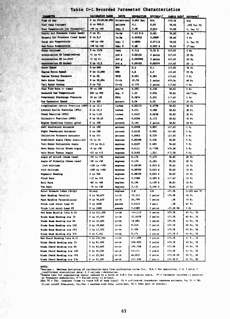
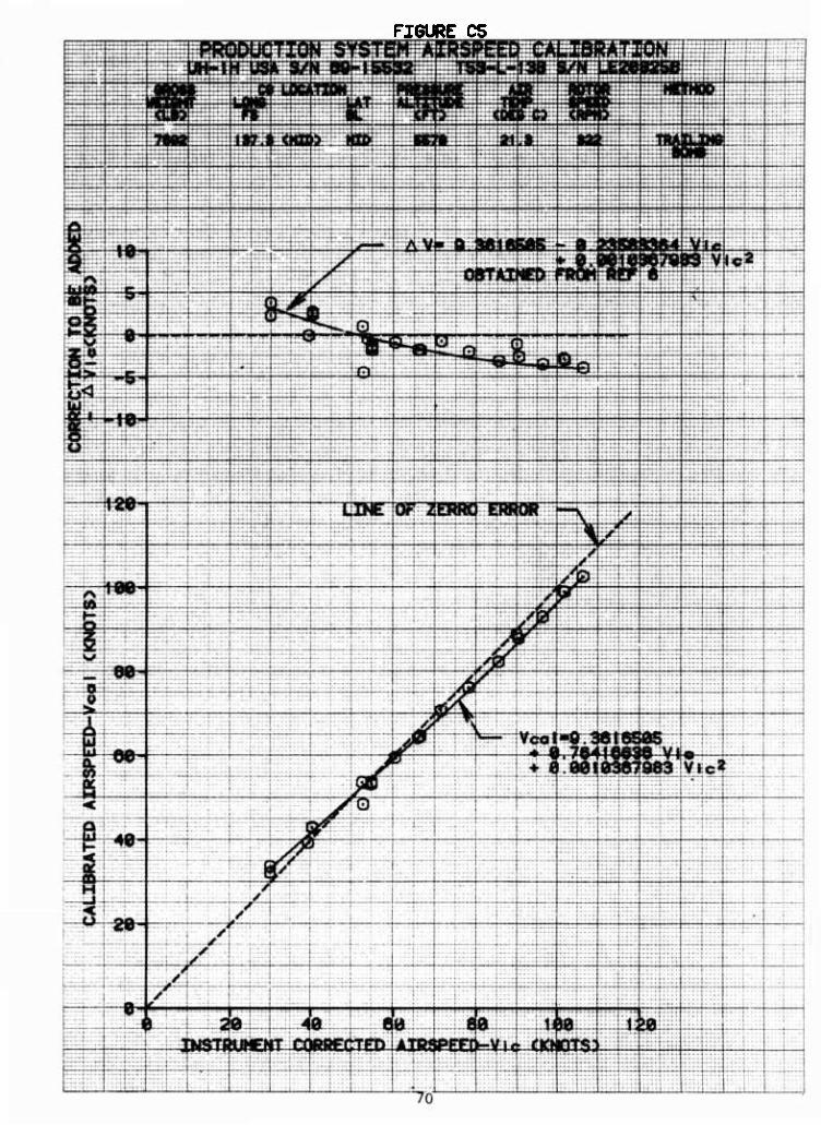
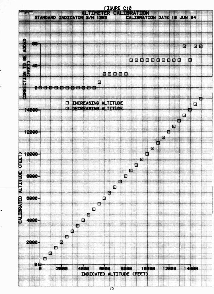
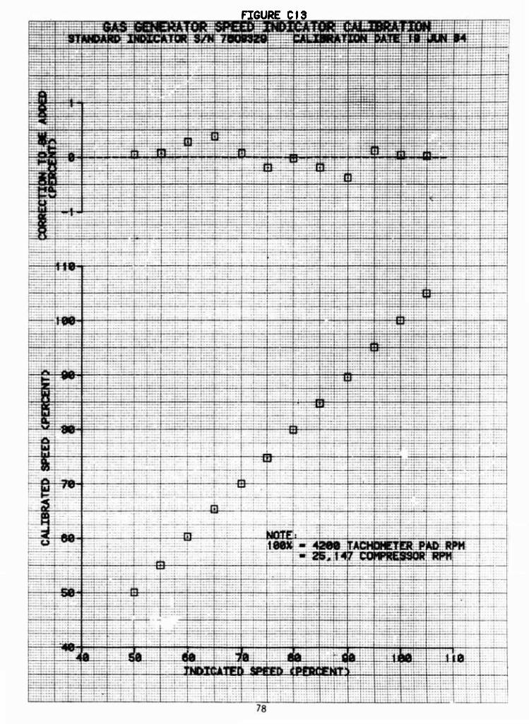
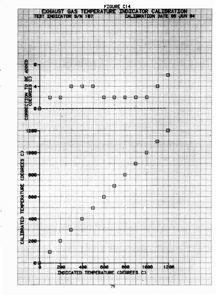
59. Calibrations for standard production indicators and systems are shown in figures C-5 through C-15, appendix C. The mission flights were planned and flown without knowledge of the calibra- tions on the part of the flight crews. The gas temperature error of four degrees C, the gas generator speed error of 0.4 percent, the torque indicating system error of 1 psl, the altimeter error of -50 feet and the airspeed Indicator error of 2 knots, while undesirable, were acceptable and had no significant
26
effect on cruise performance. The airspeed position error of +3 to -4 knots Is corrected in both the calculator and operator's nanual.
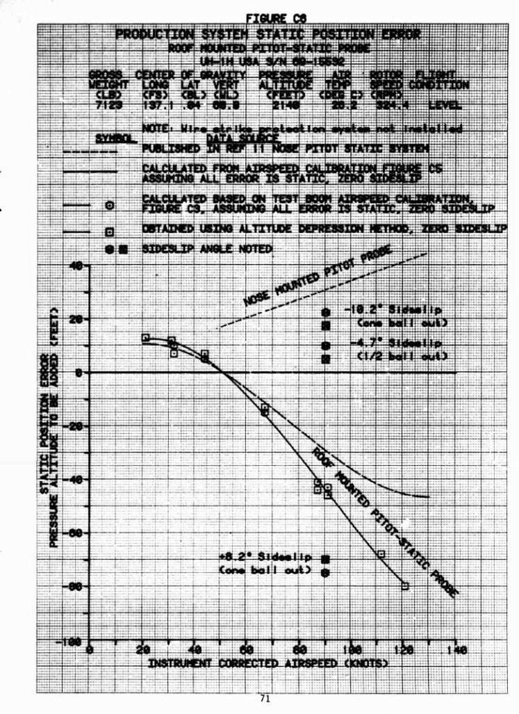
60. The static position altitude error, shown In figure C-6 appendix C for the roof mounted system, Is not significant for cruise performance. The basic position error at zero sideslip angle In level flight was as much as -80 feet.
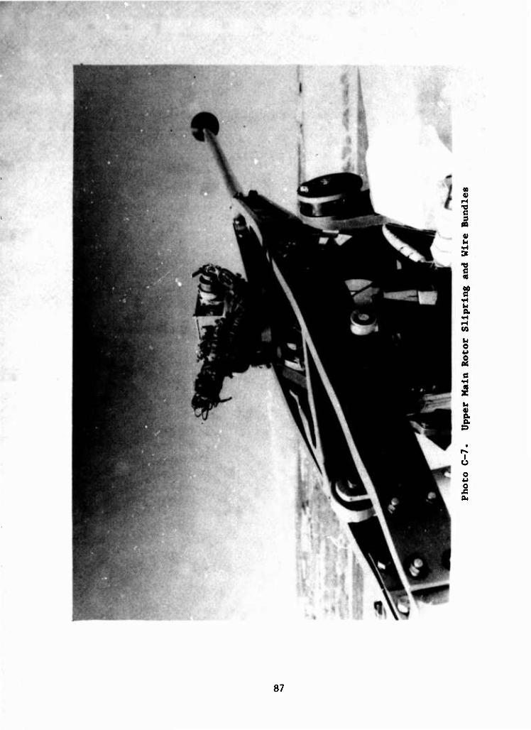
61. The fuel quantity indicating system, figure C-7, appendix C, had errors of +130 to -100 pounds (+10 to -7 percent). The system was calibrated along with the sight gage calibration. The Indicator system had relatively small errors at full and empty fuel which are the only points checked operationally. Past UH-1 fuel quantity systems have had maximum errors as small as 5 lb, limited only by the readability of the gage. Indicating that the potential accuracy is very good. The error of the system used for this project was conservative in that it indicated less fuel than actual as minimum fuel was approached. However, it was nonconservative in that it indicated lower fuel flow than actual during the first 15 to 30 minutes of flight when the fuel consumption check is made. The fuel quantity system check and adjustment procedures in the maintenance manuals are not clear or comprehensive. Required information is scattered throughout the fuel system description and trouble shooting procedures. Consideration should be given to Including intermediate points in addition to full and empty points in the quantity checks. The full fuel weight is determined by using the published full fuel volume and assumed JP-A standard density. The fuel quantity check and adjustment procedure accuracy could be improved by measuring fuel density since the ayeiem Is a capacitance system that measures fuel mass not volume. Additional information concerning fuel quantity measurement can be found in appendix D.
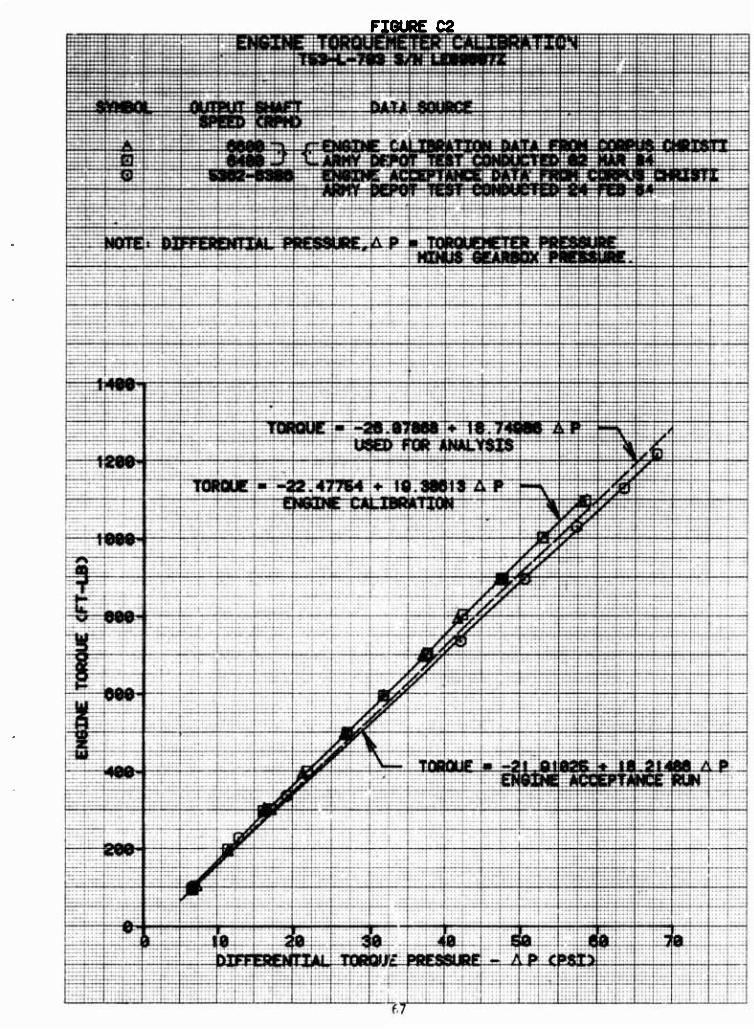
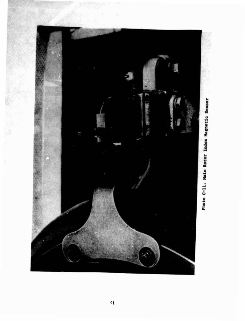
62. The engine output shaft speed calibration is shown on figure 012, appendix C. The rotor speed needle (flg. C-ll) of the dual tach has poor resolution (20 rpm increments - twice the normal operating range) and the scale Is hidden behind the engine tach needle. The engine speed indicator had an 80 tc 90 rpm error in the allowable operating range. This corresponds to a 4 to 4.5 rpm rotor speed error or nearly half the normal operating range. The error is such that true rotor/engine speed is less than indicated. This error appears in all AEFA UH-lH's. If this error is fleet wide, it needs to be corrected or component fatigue life, replacement times, performance and operating infor- mation need to be revised to reflect it.
27
Mission Flight Performance
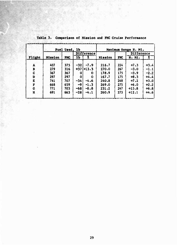
63. Time history data of mission flight conditions and performance are shown In figures I through 10 appenulx F. Mission flight performance Is summarized for each flight In table 2. Flight time Is measured from lift off to touchdown. The combined flights I-J anu L-M also Include ground time required for refueling at Palm Springs. Block speeds are the total air or ground distance divided by the total time. Fuel used Is the total fuel used from engine start to shutdown. It Includes approximately 50 lb used for start, warm up, hover-taxi, takeoff, cool down and shutdown where no distance was traveled. Weight converted to gallons using standard JP-4 density (6.5 lb/gal) Is also shown. Fuel remaining Is the total fuel remaining at engine shutdown. Specific range Is the total air or ground distance traveled divided by the total fuel used. Range to reserve fuel Is the range that would have been avallabl«» ^ad ehe flight been continued and engine shutdown occurred at nominal reserve fuel (185 lb). Range remaining Is slightly conservative In that It was calculated based on the last cruise specific range and the remaining mission fuel. Specific range would actually Improve slightly because of decreasing weight. Total available range Is the sum of acturl distance (air or ground) traveled plus the calculated remaining range. The savings presented are the differences between the performance obtained on the comparative normal and optimum profile flights. Time savings are the difference in flight times. Distance savings are the difference In flight route distances allowed by the higher optimum profile cruise altitudes. Fuel savings are the differences between total fuel used for the comparative flights.
FMC Comparison:
64. Mission flight fuel used and maximum range data are compared to FMC cruise functions data for flights A through H in table 3. The FMC fuel used and maximum range data was computed for constant cruise at the average cruise conditions of table 1 (except rotor speed) over the same distance as the mission flights, with table 1 start fuel and gross weight. The FMC cruise a..d range functions provide the only enroute fuel use data. Sufficient information Is included in the UH-1H operator's manual to more precisely compute range performance and includes idle, taxi, climb and descent fuel use. However, this is a long and error prone procedure. It could be simplified with a fully developed calculator flight planning mode. The fuel used and maximum range data show the FMC data are optimistic by as much as 68 lb and 8.8% fuel, end 15.8 nautical miles and 6.8% more range than determined from the test data. One flight was conservative by
28
Table 3. Comparison of Mission and FMC Cruise Performance
Flight
Fue I Used . lb Maximum Range N. Mi »
Mission FMC Dlfl 'erence
Mission FMC Difference
lb X N. Ml. X
A 407 375 -32 -7.9 216.7 224 +7.3 +3.4 B 279 316 +37 +13.3 270.0 267 -3.0 -1.1 C 367 367 0 0 178.9 175 -3.9 -2.2 D 297 297 0 0 167.7 175 +8.3 +4.4 E 741 707 -34 -4.6 240.8 248 +7.2 +3.0 F 668 659 -9 -1.3 269.0 275 46.0 +2.2 G 771 703 -68 -8.8 231.2 247 +15.8 +6.8 H 691 663 -28 -4.1 260.9 273 +12.1 +4.6
29
37 lb of fuel use. The difference In performance would be even larger using planning Information since actual fuel loads were as much as 170 lb less than the standard planning fuel load. The fuel use error from the FMC generally agrees with the fuel flow performance data trends (fig. 61, app F). Overall Comparison:
65. Data from the normal flight profile flights were summed and compared to the sum of data from the optimum flight profile flights. Total normal fuel use was 5007 lb. Optimum fuel use was 4060 lb, a saving of 947 lb or 19 percent. Average normal fuel flow rate was 551.8 Ib/hr. Average optimum fuel flow rate was 475.2 Ib/hr a saving of 76.6 Ib/hr or 11.8 standard gallons/ hour. Total normal flight time was 9 hours, 4 minutes. Total optimum flight time was 8 hours, 33 minutes a saving of 32 minutes. If the Palm Springs refueling time Is charged to the normal flights, enroute time difference Increase« to 3 hours, 5 minutes. Part of the time and fuel savings was obtained from the more direct flight routes available at the higher optimum altitudes (34 fewer ground miles and 28 fewer air miles). Additional benefits of the higher optimum altitude cruise are: increased gliding distance and landing area available in the event of an engine failure forced landing, improved navigational aid range (both electronic and visual). Increased communication range and generally smoother air above surface turbulence.
66. Block true airspeeds (Including takeoff, climb, cruise and descent segments) were very similar with normal flight profile yielding 99.3 knots and optimum flight profile 102.2 knots. The fuel remaining at engine shutdown represents excess weight carried on the flight which increased the fuel consumption an additional two to three percent of this weight per hour. Overall normal specific ground range was 0.1782 nautical ground miles per pound of fuel used (NAMPP) increasing to 0.2113 NAMPP for the optimum flight profile. Calculated total ground range available varied from 189 to 250 nautical miles for the normal technique and 221 to 274 nautical miles for the optimum flight profile. These all exceed the planning value of 170 nautical miles which would permit higher headwind or lower full fuel loads. A better measure of actual aircraft performance is specific air range, since it excludes the uncontrolled variables of wind, air distance and fuel load. Overall specific air ra .^e for the normal flights was 0.1799 NAMPP, and for the optimum flights it was 0.2151 NAMPP. The normal specific range Is signifi- cantly less than that calculated from reference 15 cruise specific range data and the optimum specific range is slightly less than calculated. It the approximately 50 lb of nonproductive ground fuel is subtracted, normal average specific range Increases to
30
0.1954 NAMPF and optimum Increases to 0.2323 NAMPP. The normal value approximates the calculated value, and the adjusted optimum specific range exceeds the calculated value approximately 5Z. Distance Comparison:
67. Additional information can be obtained by comparing flight profile on a destination - distance basis. The Bishop flights (E-H) show the smallest variation. This could be expected since the normal cruise altitude was closer to the optimum altitude than on other flights. Also most of the optimum flight was above 7500 lb gross weight so the more efficient 294 rotor rpm was not used. Specific air range was 0.1908 NAMPP (normal) and 0.2169 NAMPP (optimum), a 13.7 percent improvement. With the ground fuel subtracted these values increase to 0.2043 NAMPP (normal), 0.2341 NAMPP (optimum) and 14.6 percent Improvement. The Los Angeles flights (A - D) gave the best corrected specific air range and the greatest optimum profile improvement. Overall NAMPP was 0.1889 (normal) and 0.2385 (optimum), a 26.3 percent gain. Corrected for ground fuel the NAMPP was 0.2169 (normal), and 0.2887 (optimum), a 33.1 percent improvement. The Yuma flights (1 - N) yielded the lowest specific ranges, 0.1713 NAMPP (normal) and 0.2076 NAMPP (optimum), a 21.2 percent difference. Corrected for ground fuel the values are 0.1925 NAMPP (normal), 0.2291 NAMPP (optimum), a 19.0 percent difference. The lower normal specific range could be expected since the cruise pressure altitude was very low for the majority of the flight. Engine specific fuel consumption increases significantly as altitude decreases.
Climb and Descent Gains:
68. The increasing specific air range and optimum cruise gain» with decreasing distance (para 67) Indicate there is a net benefit from the climb and descent portion of the flight, compared to the cruise portion. The optimum climb and descent becomes a larger percentage of the flight as distance decreases. This apparent benefit from climb and descent can be rationalized several ways. Figure 1, appendix F shows that nearly half the flight distance is spent descending with reduced power and fuel flow, and increased specific range and vehicle efficiency, compared to the cruise. A relatively shorter time is spent climbing at higher power and fuel flow. From an efficiency viewpoint, the overall vehicle efficiency (engine efficiency times effective lift/drag) drops during the climb for a short time by an amount approximately equal to the increase during the descent over a larger period of time (figs. 1 through 10, app F). If the vehicle system is credited with the potential energy gain
31
during the climb, and debited for the descent, there Is no sig- nificant difference between climb and cruise while a smaller Increase remains during the descent. This occurs because the engine efficiency Improves substantially as power Increases which essentially compensates for the reduced lift/drag of the helicopter during the Increased power climb. The descent profile was chosen to keep the engine power, and therefore vehicle efficiency, as high as practical during the descent.
Optimum Flight Profiles:
69. The climb and descent power and airspeed schedules used for the optimum flight profile mission flights are described In appendix E. These schedules were estimated from historical data (ref 15, app A), modified for practical considerations and tested to a very limited extent during the reference 3 tests. Formal optimization methods were not used. The climb schedule consisted of a maximum power climb at an Indicated airspeed 10 knots less than the optimum altitude cruise Indicated airspeed. This produced a near maximum rate of climb at low altitude where the engine was less efficient and a decreasing rate as optimum altitude was approached. Time to climb to optimum altitude was usually less than 10 minutes. The original descent schedule was to maintain cruise power and Increase airspeed to achieve a 500 feet per minute (fpm) descent. Airspeed or vibration limits usually precluded this schedule and maximum practical airspeed with power reduced to achieve the 500 fpm descent was used.
70. The performance of idealized flight profiles shown in figure 1 was computed. These profiles included baseline cruise at sea level, constant cruise at 13,000 feet average optimum altitude, cruise climb to remain at optimum altitude from approximatly 11,500 feet to 14,500 feet, a climb cruise descent profile similar to that in references 24 and 25 including various rates of descent, the profile in appendix E, and an unconstrained series of climbs and descents. The profiles were generated for standard temperatures using specification (ref 26, app A) power available and fuel flow. Power required was derived using reference 27. Optimum altitude was determined from appendix E. A constant 314 RPM rotor speed was used and a constant 108 knot true airspeed was used for the cruise segments of the profiles. Start weight was 8000 pounds and the climb schedules described in appendix E were used for those profiles having climbs. The climb used a constant 80 knots calibrated airspeed and 1100 horsepower to approximately 9000 feet then decreasing to approximately 900 horsepower at 14,000 feet. The performance data was Integrated over 1000 foot increments for the climbs and descents and 15 minute increments for the cruise segments. Comparisons vere made by determining the distance traveled for 1000 lb of fuel.
32
DISTANCE FOR 1000 LB FUEL
CONSTANT AVERAGE OPTIMUM ALTITUDE
OPTIMUM ALTITUDE CRUISE CLIMB
OPTIMUM CLIMB-CRUISE-DESCENT AT VARIOUS RATES
• - OPTIMUM UNCONSTRAINED CLIMr AND DESCENT SERIES
Figure 1. Optimum Flight Profile Comparison
71. The constant sea level cruise gave 194 nautical miles (NM). The constant 13,000 foot cruise gave 252 NM. This decreased slightly to 250 NM for the optimum altitude cruise climb. Both references 24 and 23 altitude profiles use airspeeds near optimum cruise speed and Indicate maximum practical rate of descent is optimum for helicopters of similar size to the UH-1H. A rate of descent of 1000 fpm gave a range of 252 NM, 2000 fpm gave 265 NM, and autorotation (approximatly 2500 fpm) gave 232 NM. The original appendix E descent schedule gave a distance of 252 NM and the series of climb and descents gave 237 NM. Since these were less than expected from the mission flight results trends, a limited study at these idealized conditions was made of the effects of vertical speed on maximum specific range air- speeds and specific range. This study showed that level flight maximum specific range speed should be increased approximately one knot for each 100 fpm rate of climb and decreased one knot for each 100 fpm rate of descent. The appendix E descent schedule was revised to reflect this result so that descent airspeed should be decreased 10 knots from level speed for the Army stan- dard rate of descent of 1000 fpm. Using this revised schedule Increased the appendix E profile distance to 263 NM. The series of climbs and descents was modified further to climb at maximum
33
range level speed (after the Initial climb) and descend at 500 fpm, 5 knots below best level speed. This improved the distance to 278 NM. While the gains from these climb and descent profiles are small, they do shew that no net penalty is paid for climb and descent, as long as airspeed and power are near optimum. True optimum profiles are likely beyond the capability of a calculator and would require ground based computer solutions. This would be enhanced if the computer had direct access to weather data (temperature and wind variation with altitude). Such solutions could then be loaded into the calculator.
PERFORMANCE TESTS
72. Level flight performance and limited hover performance tests were made to supplement the data of the reference 3, appendix A tests. The overall objective is to develop a mathematical per- formance model that can be used in the calculator and has flight test and theoretical basis. Such a model will be required to achieve acceptable accuracy for individual aircraft under opera- tional conditions. The general approach to date has been similar to tha'c of reference 28. This analysis uses an empirical charac- terization of blade stall and compressibility effects. A com- pressibility characterization based on potential flow compressi- bility correction has been developed and independently refined in reference 27. It can duplicate the reference 3 data within one percent. However analysis of reference 15 data indlca es this correction is increasingly inaccurate above thrust coef c- ients of 0.00A, the limit of reference 3 data. A thrust coef c- icnt of 0.004 approximates optimum altitude conditions. The sensitivity of compressibility effectä to thrust coefficient increases nonllnearly above this value and stall effects may become significant. Emphasis during this test was on the higher thrust coefficients. Use of a higher powered T53-L-'/ü3 engine enabled tests over a larger range of conditions.
Level Flight Performance
73. Level flight performance tests were conducted at thrust coef- ficients from 0.004 to 0.0052, referr«>H rotor speeds from 300 to 350 rpm, and airspeeds from minimum indicated airspeed to limit airspeed. The tests were all flown at zero indicated sideslip and a mid longitudinal and lateral c^. Data are showu in figures 11 through 54, appendix F. For each test two figures are presented.
34
Hover Performance
74. Out-of-ground effect hover performance tests were conducted at the hot and cold weather test sites to expand the rotor tip Mach number range. The free flight technique was used and winds were less than 3 knots. Nondlmenslonal rotor and engine power coefficient data are shown on figure 35. Engine power coefficient data corrected for compressibility and linearized are shown on figure 56.
Engine Characteristics
75. Engine performance parameters recorded during these tests Included torque, fuel flow, measured gas temperature, gas genera- tor speed and output shaft speed. These parameters were "referred" using relationships obtained from the engine manufacturer. With the exception of Inlet temperature rise. Installation conditions were taken from reference 15. The Inlet temperature rise used was three degree C. Reference 17 analytically determined a rise of 2.9 degree C, for a very similar Inlet. Referred engine chara- cteristics data are compared to the engine calibration data and predictions from the engine model specification computer programs on figures 61 through 67, appendix F. The model specifi- cation performance was determined using references 26 and 32, appendix A for the T53-L-13B and references 31 and 33 for the T53-L-703 engine. Reference 33 results are suspect In some areas and are being updated.
Power Available
76. Military and continuous power available for the T53-L-13B engine were derived from the engine specification. The data and the Installation losses used are shown on figures 68 and 69, appendix F. Maximum test engine power agreed well with figure 68 when a three degree C inlet temperature rise was used- Military and continuous power for the T53-I.-703 derived from the engine specification are shown on figures 77 and 78. This pov/er avail- able data has some anomalies and is suspect because of discontinu- ities with altitude and temperature and inability to run at some allowable condition. Maximum power f..cm the T53-L-703 engine could not be tested within the test conditions because of drive train limits. A relatively simple mathematical model of power available is derived in reference 17, appendix A. This model is analogous to the operation of the "Nl bias" curve of the T53 fuel control. It should be suitable for a calculator power available function, particularly if it is corrected to an individual engine baseline.
35
Fuel Flow
77. The engine model specification fuel flow for the T53-L-13 at three different output shaft speeds is shown on figures 70 through 73, appendix F and for the T53-L-703 on figure 79. Fuel flow is shown as a function of power and altitude at 0 degree C, with an independent function of the variation with temperature. Operator's manuals for the T33 indicate the fuel flow variation with temper- ature is one percent for each 10 deg C deviation from zero. This variation along with other parameters is presented on figures 74 and 80 for each engine. Fuel flow variation with temperature was found to be more consistently described by fuel flow per horsepower. These data are shown on figure 75 for four different output shaft speeds for the T53-L-13 engine and summarized on figure 76 as a function of referred output shaft speed. Calibra- tion and test data are also shown on figure 76 where fuel flow variation with temperature and total fuel flow are a strong function of output shaft speed. This same approach to defining fuel flow deviation was applied to the referred fuel flow data, figure 61, to produce a deviation of measured T53-L-13 fuel flow from specification fuel flow on figure 62. While the data do show a large difference from specification fuel flow, they also show relatively consistent trends with power, referred output shaft speed and altitude. This indicates that a simple fuel flow model could be derived using the model specification as a bpsls. The test data also show that the fuel flow improvement with altitude is not as large as the model specification would predict except at very high referred power. The unlnstalled engine test cell calibration data, obtained near sea level stan- dard conditions, agree well with the engine model specification. This difference between test and calibration data indicate that the model specification does not accurately predict the effects of altitude or that Installation losses are Incorrect. Engine Installation losses for the current UH-1H configuration should be determined by test. This same analysis was not done for the T53-L-703 engine.
36
CONCLUSIONS
GENERAL
78. The FMC performance calculator has the potential to facilitate flight planning, Increase mission performance, and provide greater safety. A form of "regressive" analog modeling in which the program Is updated with Individual aircraft data may be required to achieve acceptable accuracy. The calculator program evaluated has many good features and functions which should be retained In future programs. It needs significant Improvement In the areas of planning, complexity. Instructions and calculating speed. Improvements will require additional memory and perhaps a more advanced calculator.
SPECIFIC
79. The following conclusions were a result of the FMC calculator evaluation:
a. The calculator program accurately reproduced the source data from which the functions were derived (para 22).
b. The calculator high output precision was erroneously perceived by most evaluation pilots to be a measure of the accuracy (paras 15 and 21).
c. A one percent overall accuracy Is desirable and acceptable. To achieve this accuracy will likely require that Individual aircraft data be used to update the program for engine, aircraft and measurement system variation. The HP-41CV system is capable of automatic data input (paras 23 and Al).
d. The calculator execution time was more than two minutes for some functions. Five seconds from last input to first output would be an acceptable execution time (para 16).
e. The absence of a planning mode to integrate and accumulate results from each flight phase, the absence of some data such as idle fuel flow, and the slow execution resulted in longer times to plan a flight using the calculator than using the operator's manual (paras 16, 33 and Al).
f. The calculator was much easier to use in flight than the operators manual (para 15).
g. Because of the calculator physical characteristics, it was difficult to avoid erroneous data input in flight (para 19).
37
h. The weight and balance function was well designed and required minimum Input while quickly providing most needed output. It needs some refinement, such as load limit checks, for opera- tional use (para 32).
1. Input termination or option selection, determined by Input value, such as terminating loading Input by inputing zero load, Is a good concept (para 27).
J. The units used were proper, however their Inclusion In the limited HP-41 display decreased the readability (para 24).
k. The limit checks were good and comprehensive. Their mech- anization needs improvement (para 26).
1. The use of the program could be simplified if maximum performance values such as maximum range or maximum hover weight were provided as default upon input request (paras 26, 28, 29 and 35).
m. Takeoff performance could be added to the hover performance function (para 36).
n. Time, distance and fuel used during climbs and descents at any power and airspeed are not provided and are needed for accurate range and endurance determination (para 37).
o. FMC fuel use and range data are optomistic by as much as 8.8 percent fuel use and 6.8 percent range (para 64).
p. The temperature prediction algorithm can result in signif- icant errors based on temperature - altitude profiles observed during this test, (para 44).
q. The wind computation for groundspeed was in error (para 39).
r. The indicated to pressure altitude conversion was In error (para 24).
80. The following conclusions were a result of the mission flight tests:
a. A 19 percent fuel savings was achieved using optimum cruise flight profile at temperatures approximately 15 degrees C above standard. Greater savings can be expected at colder temper- atures where compressibility effects Increase (paras 52 and 65).
38
■
• " ■
b. True optimum cruise altitude and airspeed are significant- ly affected by winds and wind gradients wivh altitude (paras 55 and S3).
c» Optimum climb and descent profiles do not decrease range performance and may improve it, as long as airspeed and power schedules are near optimum (para 71).
d. Aircraft lateral attitude during fueling significantly affects fuel capacity (para 48).
81. The following conclusion was reached as a result of the performance tests and data analysis:
a. A compressibility correction algorithm predicts past UH-1H fuel conservation power required data within one percent up to optimum altitude. It is inaccurate above optimum altitude and needs further development (para 72).
b. A simple and accurate power available model, adjustable to individual engine performance, is feasible (para 76).
c. A simple and accurate fuel flow model is feasible (para 77).
82. The following conclusion was made regarding the UH-IH: The engine power output shaft speed tachometer system appears general- ly in error by 80 to 90 rpm (para 62).
39
RECOMMENDATIONS
83. The following recommendations are made with regard to future performance calculator development.
a. Future performance calculators must have a planning mode that runs more or less automatically, requires a minimum of computer knowledge and Instructions and produces at least the minimum Information required (paras 16 and 41).
b. Future performance calculators should accurately compute performance for any conditions at which the aircraft can operate so that major modifications are not required as limits or operat- ing procedures change (para 25).
c. The calculator should allow determination of performance for conditions beyond operating limits that are under the control of the pilot. Those limits not under the pilots control should be absolute (para 26).
d. Consideration should be given to providing several levels of input and output parameters, with the lowest (default) requir- ing and providing a minimum of information and the highest being established by the user to meet his specific requirements (paras 27 and 30).
e. If the HP-41CV is used for future performance programs, an auxiliary display should be considered (para 20).
f. Emergency performance, such as autorotation, should be included in future calculator programs (para 40).
g. The effects of winds on maximum range airspeed and alti- tude should be Included in future calculator programs (paras 55 and 58).
h. Some method of updating power available with service time and engine condition should be Incorporated in future performance calculators (para 22).
i. The estimated accuracy of major parameters should be Included in future calculators operator's manuals.
J. The current UH-1H operator's manual directional control data should be corrected for the rotor/engine speed indicator error and used in future UH-1H performance calculators (para 22).
84. The following recommendations are made with regard to UH-IH manual changes or additions:
40
a. Include In the operator's manual tint effect of lateral attitude on fuel capacity (para 48).
b. Include in the operator's manual the instruction to use the fuel quantity indicator when more precise performance planning is required (para 44).
c. The fuel quantity system accuracy checks and instructions need improvement. The test aircraft met these checks with a ten percent error (para 61).
d. Research current use of non-crashworthy fuel systems throughout the fleet. If there are none, delete all information and references to them from the manuals and future calculator programs (para 32).
e. The effects of winds on maximum range airspeed should be included (para 55).
f. The current UH-1H operator's manual directional control data should be corrected for the rotor/engine speed indicator error (para 22).
85. The following recommendations are made regarding studies of the UH-1H helicopter:
a. The engine installation and accessory losses of the cur- rent configuration UH-1H should be determined by tests (paras 75 and 77).
b. The generality of the output shaft speed (N2) tachometer system error needs to be determined. If it is fleetwide, the error should be corrected or else the performance and operating information needs to be revised (para 62).
41
APPENDIX A. REFERENCES
1. Letter, DAVTE-M, USAAEFA Project 81-0i-l, subject: Report, Fuel Conservation of US Army Helicopters, Part 1 Flight Operations Improvement Anaiysi-, 28 January 1982.
2. Letter, USAASFA Project 81-01-2, subject: Report Fuel Con- servation of US Army Helicopters, Part 2 Development and Evalua- tion of Fuel Conservation Formatted Data, 23 October 1981.
3. Final Report, USAAEFA Project 81-01-3, Fuel Conservation of US Army Helicoptere, Part 3 UH-1H Flight Testing, August 1982.
4. Final Report, USAAEFA Project 81-01-4, Fuel Coneervation of US Army Helicoptere, Part 4 OH-58C Flight Testing, August 1982.
5. Final Report, USAAEFA Project 81-01-5, Fvel Conservation of US Army Helicopters, Part 5 AH-1S Flight Testing, January 1983.
6. Final Report, Number 205-099-158, UH-1H Flight Management Calculator Field Evaluation, Bell Helicopter Textron, September 1983.
7. Letter, AVRADC0M, DRDAV-DI, Subject: Test request No. 81-01-6, Fuel Conservation of US Army Helicopters, Part 6, Performance Calculator Evaluation, 21 September 1983.
8. Letter, DAVTE-M, Subject: Test Plan, USAAEFA Project No. 81-01-6, Fuel Conservation of US Army Helicopters, Part 6, Performance Calculator Evaluation, 18 November 1983.
9. Technical Manual, TM 55-1520-210-10, Operator's Manur.L, US Army Model UH-lD/fl Helicopters, with change 13, 25 August 1971.
10. Technical Manual, TM 55-1520-210-10, Operator's Manual, US Army Model UH-1D/H and EH-1H Helicopters, 18 May 1979, with change 19, 1A March 1984.
11. Technical Manual, TM 55-1520-210-10, Operator's Manual, US Army Model UH-1H/V Helicopter, 15 July 1985.
12. Detail Specification, Bell Helicopter Textron, No. 205-9A7- 177, UH-IH Utility Helicopter FY-74 Procurement, 15 May 1973.
13. Manual, HP-41 Owner's Handbook and Progrvurming Guide, Hewlett- Packard Company, September 1980.
14. Letter, AVSCOM, DRSAV-E, Subject: Airworthiness Release for UH-IH S/N 69-15532 for USAAEFA Project 81-01-6, et al 16 January 1984, with revision 2, 26 July 1984.
42
15. Final Report, USAAEFA Project 66-04, Engineering Flight Teat of the YUH-1H Helicopter (Phase D Limited), November 1970.
16. letter, AVSCOM, AMSAV-GR (R-MCP), Subject: Aviation School Requirements for Performance Data Changes for Mission Planning, 25 June, 1969.
17. Final Report, ÜSAAEFA Project No. 73-01, Helicopter Lift Margin Syetem and SloD Speed Performance Evaluation, August 1977.
18. Manual, Bell Helicopter Textron, Performance Data Quick Flight Management Calculator Ueer'e Guide, Version 3, Release 0, 19 April 1983.
19. Article, AGFA Pilot, New Product Evaluation: Beech Aircraft Corp. Flight Planning Calculator, September 1980.
20. Article, United States Atmy Aviation Digest, Atmoepheria Sciences Laboratory: Weather Intelligence Enhancee Capabilitiee, April 1985.
21. Field Circular, US Aviation Center, FC 1-211, Aircrew Training Manual, Utility Helicopter, UH-1, 31 July 1984.
22. Final Report, USAARL Report No. 84-6, In-Flight Evaluation of Two Molecular Sieve Oxygen Concentration Syeteme in US Army Aircraft (JUH-1H and JU-21G), March 1984.
23. Technical Paper, Kathy H. Abbott and Charles E. Knox, NASA 2383, Reference Energy-Altitude Deeoent Guidance, January 1985.
24. Technical Memorandum, G. L. Slater and H. Erzberger, Optimal Short-Range Trajectoriee for Helicopters, NASA TM 84303, December 1982.
25. Technical Paper, G. L. Slater and M. Stoughton, 0n-Line Determination of Optimal Flight Paths for Helicopters, American Helicopter Society Symposium, May 1984.
27. Technical Memorandum, Dr. R. Macmillan, Leigh Instruments Limited, AISLIS: Modification of USAAEFA Compressibility Algorithm to Fit UH-1H Helicopter Performance Curves, November 1, 1983.
43
28. Technical Paper, Barclay Bolrun, Generalising Helicopter Flight Teet Performxnoe Data, Proceedings, American Helicopter Society Symposium, May 1978.
29. Proposal, Bell Helicopter Textron, Composite Main Rotor Blade for UH-1H Helicopter, number 205-199-602 Vol. 6, Part 2 perfor- mance, March 1982.
30. Final Report, USAAVLABS TR 68-57, Inetallatian of a High- Reduetion~Ratio Tranemieeion in the UH-1 Helicopter, May 1969.
31. Model Specification, Lycomlng Division, Avco, TS3-L-703 (LTC1K-4G) Turboehift Engine Specification No. 104,43, May 1974, Revised February 1981.
33. Computer Prcgram, Lycomlng Division, AVCO, Eetimated Steady State Pe formance Computer Program, File No. 19.04.32.00 Received December 1981.
44
APPENDIX B. FLIGHT MANAGEMENT CALCULATOR AND AIRCRAFT DESCRIPTION
FLIGHT MANAGEMENT CALCULATOR —_____^——^^_—_—
1. The flight management calculator (FMC) consists of the
Hewlett-Packard HP-41CV programmable scientific pocket calcula- tor, hardware modifications to the calculator, and the program, "Performance Data Quick (PDQ)" version 3, release 1.
Calculator
2. Overall dimensions of the HP-41CV calculator are 5.6 X 3.1 X 1.3 Inches. This size and the light weight of 8 ounces make It very portable. The size makes It easy to mount on the standard kneeboard and still leave room for notes. However, the face is small and the 39 keys are small and closely spaced. A tactile "click" indicates key activation which requires approxi- mately 5 ounces of force. The built-in display consists of 12 alpha or numeric characters scrollable to a maximum of 24. The scroll rate Is two per second so a full message would take 6 seconds to display completely. The characters are generated from a 14 segment liquid crystal display (LCD) so the number and legibility of the characters are limited. Neither the dis- play nor the keyboard has lighting. The calculator is powered by 4 size N batteries which last approximately six months, or a rechargeable battery pack. The calculator has Federal Communications Commission (FCC) approval for use in aircraft. The basic HP-41CV was augmented with three random access memory (RAM) chips which give It approximately 6500 eight bit bytes memory capacity. A bytr of memory will store one alpha or numeric character or approximately one program step. A sign, decimal exponent and ten-digit constant, the calculator precision, can be stored in a 7 byte register. The calculator also has more than 200 mathematical and system functions available that can be directly executed or executed under program control. The calcu- lator may be interfaced with printers, computers and many other peripheral devices.
Modifications
3. The FMC modifications include: a key cap to prevent switching into program mode, which could cause alteration of the program; paint blanking of the normal HP-41CV key function labels; a custom key label overlay; velcro backing for attachment to the pilot's kneeboard; and a chip cap to prevent demounting the extended memory chips which would cause loss of the program from memory. The chip cap would not be required on a production system as the program would be written on "programmable read only memory" (PROM) chips, which would preclude loss or alteration of the program by the user. Program memory and, therefore,
45
program capability could be greatly expanded by adding PROM chips. PROM chips up to 3200 bytes are available which would provide more than 20 times current program capacity when installed in all four available ports.
Program
4. The program, PDQ, generally duplicates the performance and weight and balance information currently in the UH-1H operator's manual (ref 11, app A). Information not currently available in the operator's manual that can be obtained from PDQ includes: optimum cruise altitude, hover endurance, pressure altitude calculated from indicated altitude, cruise ground speed, and power assurance calculations which predict compressor speed and exhaust gas temperature relation to torque. Information that is available from the operator's manual but not included in PDQ include: autorotation performance, takeoff performance, idle fuel flow, optimum cruise airspeed, cruise performance below 85 knots, climb, and descent, (except maximum endurance fnd maximum climb performance which are included in PDQ). The PDQ program contains no information on optimum airspeed, rotor speed, wind effects on optimum conditions or optimum climb and descent, power and airspeed schedules. The program is thoroughly documented in reference 6. The documentation includes the functions used to describe each type of performance (generally fifth order poly- nomials) and compares them to the source data. The program is coded in KP-41 calculator language. Particular features of the program are discussed in more detail in the results and discussion section of this report.
TEST AIRCRAFT
5. The test aircraft, production UH-1H, USA S/N 69-15532, is shown in photos B-l through B-8.
Weight and Balance
6. Prior to testing, the aircraft empty weight (including full oil and undrainable fuel) and horizontal center of gravity (eg) location were determined with calibrated scales. Vertical eg was determined by suspending the helicopter from the top of the rotor mast and measuring the resulting attitude. The empty weight was 6024 lb including approximately 900 lb of test instru- mentation. The eg was fuselage station (FS) 147.887, butt line (BL) 0.005, waterline (WL) 67.194. Total fuel capacity in a level attitude was uetermined to be 207.2 gallons from a fuel drained condition. Unuseable fuel is stated as 1.5 gallons giving a total useable capacity of 205.7 gallons.
46
> V «
u u u
i
5
47
\ /
3 •H >
£
u «
CO
P>4 I
O £
48
I
00 •H «i
I
u u
(0 s m i
5
49
u « 4J kl
s Or
u 0)
OS
00
I
« u u I-
I o a.
50
51
9 01
u
u a <u
OS
CO u o u
09 0)
I pa
I
52
•o Ui
V
u u
gg
H
I pa
o
Pu,
53
54
Control Rigging
7. The following main rotor tip static blade angles were measured with the collective control full down, rotor mast vertical, rotor hub horizontal and stabilizer bar horizontal:
Cyclic Position Tip Blade Angle (degrees)
Rotor Longitudinal Lateral
Neutral
Azimuth o8 90° 180° 270°
Neutral +0.80 - 1.00 -3.00 - 1.22 Full Forward Neutral +1.74 -13.25 -3.12 +10.37 Full Aft Neutral -2.32 + 9.80 40.92 -12.55 Neutral Full Left +9.00 + 2.30 -11.70 - 4.35 Neutral Full Right -9.69 - 1.10 + 7.10 - 0.83
Note: Reference rotor azimuth (0°) Is aft.
a. The variation of average tip blade angle with collective position was:
Collective Position (%) 0 25 50 75 100
Avg. tip blade angle (deg) -1.11 +2.03 +5.85 +9.70 +12.67
b. The average blade pitch to flap angle coupling was -0.052 degrees/degree over the full flapping angle variation of 23.2°.
c. Mast angle forward tilt with the aircraft in a level attitude was 5.1 degree« and lateral angle was zero degrees. Transmission mount stiffness (determined during the vertical eg measurement) was approximately 100,000 in.-lb moment/degree deflection about an assumed pivot of FS 140.249, WL 59.433.
d. The tail rotor was rigged several times during the project as the instrumented tail rotor gear box was installed for engineering tests and removed for ferry flights etc. The installation and rigging were done per applicable maintenance instructions and met operational rigging checks but varied substantially. Full left pedal blade angle varied from -15.9 degrees to -19.0 degrees. Blade angle travel measurements varied from 23.5 to 24.1 degrees. Blade angle measurements were averaged for each blade at each flapping stop with ground hydraulic power applied. Without hydraulics, maximum blade angle is reduced approximately 0.5 degree at each stop (1.0 degree travel reduction). Dynamic blade angle limits in flight are known to vary significantly from static ground measurements.
55
This variation was not determined. The last rigging (applicable to the mission and hot weather performance flights) was: full left pedal blade angle ■ -18.9 degrees; full right pedal blade angle +4.6 degrees. Tail rotor flapping stops were set at +7.5 degrees.
e. The synchronized elevator rigging measured on the top (flat) surface relative to the aircraft reference line was:
Left Side Right Side
Full forward cyclic +2.7 degrees +4.0 degrees Full aft cyclic -0.3 degrees +1.0 degrees Maximum nose down -2.9 degrees -1.7 degrees
(approximately 40Z from full fwd cyclic)
Note: This rigging is approximately 0.6° nose down from nominal.
External Instrumentation
8. Several items of external test Instrumentation probably increased the parasite drag of the fuselage and profile drag of the rotor compared to an operational aircraft In clean configur- ation. The amount of drag increase was not determined. These items included: test airspeed boom Including yaw and pitch sensing (YAPS) head and ram air temperature probe, dew point sensor, tall rotor slip ring assembly, tail rotor collective potentiometer and cover, main rotor slip ring assembly, hub instrumentation and wiring harness, main rotor blade strain gages, and paint zone markings (for icing te;.ts). These items are shown in photos C-l through 014, appendix C. Additionally, the main rotor blades had significant leading edge erosion and numerous (accept- able) dents, having accumulated 2205 hours of their 2500 hour retirement life. From a drag standpoint, the test aircraft is probably representative of a worst case fleet UH-1H in clean configuration, with the possible exception of those with rotor infrared radiation (IR) suppressive paint.
Standard Configuration Variation
9. There is a wide variety of modifications and equipment instal- led in operational ITH-IH helicopters that may affect performance or operating characteristics. Some items are Inherent differences, such as the airspeed systems; some are in the process of being retrofitted to the fleet, such as the wire strike protection system; some are currently in development and may be Incorporated In the near future, such as the composite m^in rotor blade. The
56
only significant change made to the test aircraft during this project was the replacement of the standard T33-L-13B engine with the T53-L-703 engine for the hot weather tests. This resulted In empty weight Increase of 9.5 lb and a slight aft shift In the eg. The T53-L-703 engine has been designated as a contingency t.igine for the UH-1H. The T53-L-13B has been out of production for several years and spares are In short supply. A preliminary airworthiness evaluation (USAAEFA Project No. 84-25) of this configuration Is In progress. The test aircraft configuration and known alternative configurations are listed In table B-I. Design data, data derived from design data and flight limitations applicable to these tests are tabulated In tables B-2, B-3 and B-A, respectively.
Installed Installed Installed Installed Flat black on olive drab Black on olive IR suppressive Flat black IR suppressive Black & white hi-visibillty Installed Installed Various armament Auxiliary fuel Dispensers Standard plus H F comm on tall boom Global positioning Various mission antennas
58
Overall Dlaensioni Length (rotor turning) Length (note to tall) Width of skids (max width except rotor) Height (to top of turning tall rotor) Height (to top of rotor mast) Fuselage ground clearance (dejlgn weight) Main rotor clearance (rotor tip to tall
boom, static) Weights
Empty weight (typical fleet aircraft) Design gross weight Maximum gross weight Allowable test weight (ref 14)
Main rotor Type Rotation direction Number of blades Rotor diameter (blades) Rotor diameter (Including tracking tips) Blade length Blade chord Blade twist (hub center to tip) Blade airfoil Preconlng angle Hub diameter Mast angle (from vertical ref) Control travel: (measured at center of grip)
(replace drive train and rotor) Output shaft speed:
Maximum steady state Minimum steady state Minimum steady state below 7500 lb Maximum transient (below 9IZ N})
Exhaust Gas Temperature (T53-L-13B) Continuous 30-mln limit starting and acceleration (10 sec) Maximum for starting and acceleration
Turbine Gas Temperature (T53-L-703) Continuous 30 minute limit Starting and acceleration (5 sec)
Gas Producer Maximum speed - T53-L-13B 25,600 rpm (101.5X) Maximum speed - T53-L-703 26,650 rpm (106.OX)
Rotor Speed Maximum power on 324 rpm
Power on transient 331 rpm Power off 339 rpm
Minimum power on 314 rpm Power on less than 7500 lb 294 rpm Power off 294 rpm
Airframe Loading: (see ref 11 for center of gravity envelope)
Maximum overload weight 9500 lb Maximum floor loading 100 lb/ft2
Maximum cargo hook capacity 4000 lb Maximum forward eg Sta 130 Maximum aft eg Sta 144 Maximum lateral eg +5 in.
Limit load factors: Design positive 6600 lb ■l-3.0 g
9500 lb f2.1 g Minimum for flight +0.5 g
Airspeed: (see ref 11, for complete airspeed envelope) Forward flight maximum 123.6 KTAS at 2000 ft Sideward and rearward flight maximum 30 kt
50 psi 50 to 54 psi 54 to 61 psi Over 61 psi
6600 rpm 6400 rpm 6000 rpm 6750 rpm
400oC to 610' 'C 610oC to 625' C 6250C to 675e C
760' •c
400oC to 820e C 820oC to 880' C 880oC to 950° C
61
APPENDIX C. TEST INSTRUMENTATION
1. All instrumentation was Installed, calibrated and maintained by US Army Aviation Engineering Flight Activity (USAAEFA) except for strain gages. The main rotor blade, hub, and mast and tall rotor torque strain gages were Installed and calibrated under contract by Bell Helicopter, Textron. The main rotor blade Instrumentation consisted of five strain gage arrays at each of five radial stations; one gage at the leading edge, two gages (top and bottom) near the 1/4 chord point and two gages (top and bottom) near the trailing edge. The gage array signals were resolved, calibrated and output as two parameters, beam (flapwlse) bending and chord (edgewise) bending for each radial station. All Instrumentation Including sensors. Indicators, signal con- ditioning, pulse code modulation (PCM) encoder, recorder, telemetry and all mounting hardware weighed approximately 900 pounds. PCM data were recorded on a wide-band analog tape recorder aboard the alrcr-ft. A 12-blt encoder formatted with 34 main frame and eight deep sub-frame columns operated at 192 kllo-blts per-second (KBPS) rate yielded a main frame rate (MFR) of 470.38 samples per second per word, which was recorded on one of 14 tape tracks at 13 Inches-per-second (IPS). For the mission test flights data rate was reduced to 50.4 KBPS, for a main frame rate of 125 samples per second per word, recorded at 3-3/4 IPS to conserve tape. An Intervalometer was used during the mission test flights to take 30 second long records, at five minute Intervals during cruise and at one minute Intervals during other flight phases.
RECORDED PARAMETERS
2. Calibration and dynamic characteristics of the recorded parameters are listed In table C-l. Resolution is the "engineering value" change per PCM count. For some parameters multiple channels were used to Improve the dynamic range. A "residual" is the maximum engineering unit deviation of the calibration data from the calibration curve fit and gives an indication of the remaining systematic error due to curve fitting. Those parameters labeled "S", indicate a voltage substitution calibration. The "response" gives 3 db filter cutoff frequencies in hertz where applicable. In addition to PCM recording, two parameters (pitch link load #2 and chord bending station 192) were recorded in parallel on separate tape tracks using frequency modulation (FM) to aid in reconstruction and analysis of the waveform derived from the PCM data.
62
Table C-l. Recorded Parameter Characteristics rAMMTU CAUSMTIOM »AWCI UNITS MSOWTIO« «PS1IHIA'.' SAMFLE HATE' SISPONSE1
Tl« of D.r 0 ta 2):J«iJ«.m hnalniaac 0.001 Sac N/A 470.31 N/A
Naat »•;idl;i(i Parallal 0 to 3»,«70 l.i-lb 18.313 2 point 470.5« 40 re
Haat landln« Parpandlcular 0 to 3«,630 In-lb 2*.7«« Z point .58 40 re
Pitch Link Aalal Load »1 0 to 2*00 pounda 0.03*5 3 pot.i .58 60 re
Pitch l.li.k Ailal Load K 0 to 2*00 pounda 0.038« 3 point .70.58 PM 5 Ft
Hub laaa landl.ip (ata *.}) 0 to 111,300 i.i-lb IU.1I2 2 point 470.58 60 Pc, 5K
ilada iaaa («ndlitf aca It 0 to *0,D00 In-lb 32.0*5« 2 point 470.5« 60 Pc, 5«
llada laaa Mndl.tn aca It 0 to 31>*00 l.i-lb 18.88* 2 point 470.58 40 Pc, 5K
llada laaa landln« ata 1 Vj 0 to 1»,«»0 In-lk «.2A] 2 point 470.58 »0 re, 5«
llada laaa laudlni ata 1*2 0 to 12,300 In-lk 8.088 2 point 470.58 60 re, 5K
llada laaa Sandln« aca 23* 0 to 5,162 <n-lk «.*7t 2 point 470.58 P 60 re, 5«
Hub Chord landln« (ata b.l) 0 to 230,OOU i.i-lb 2'i:.299 2 point 470.58 40 P.-, «
llada Chord Saudlnf ata 15 0 to SI,000 In-lk 50«.«2« 2 point 470.58 40 Pc, 5«
llada Chord laadl.-ig ata 14 0 to »3,600 l.i-l» H*.T08 2 point 470.5« 40 Pc, 5«
llada Chord Sanding ata IV) 0 to *0,200 in-ib 53.07* 2 p .in 470.5« 60 re, 5K
Slada Chcrd Sanding ata 1«2 0 to 23,3*0 In-lb *».833 2 point 470.3« PM 60 re. 5K
Slada Chord Sanding ata 23A 0 to 10,500 m-lb 107.358 2 poi.it 470.58 F 60 Fr, 5K
NOTES; Uaildua.t NaxlMiB daviadon of calibration data fro» calibration curve Ht» N/A - Not applicabl«; 2 or ) poi.tt * iiiauffUi«nt «tatistical data; S - voltaM "ibaclCuclon.
'Saapla rate for e>ifir>«*r 1 i« taata; raduead by a ratio of 3.0:1 for «iaaloit taata. FM • Paranectr recorded lit paraltcl by frequency soduiation; F - Failed early i* project.
]Sac TC - T1L. onatanr (tiaa to r-ach 63Z of step Input) Ft - unfiltarad tranaducar rasponaa aatiaata, ht; Fc • )db filter cutoff frequency. hi;/Sec a »axinun alcv rate, unita/aec; )K - )Khc part of prolcct.
63
SYSTEM CALIBRATIONS
3. In addition to transducer calibrations, the engine torquemeter calibrations were obtained from engine test cell calibrations conducted at Corpus Christi Army Depot, Texas. There was an apparent discrepancy in the T53-L-703 calibration which is dis- cussed in appendix D. The torquemeter calibrations are shown in figures C-l and C-2 for the two engines used. The test air- speed probes and production airspeed systems were calibrated for position error. Results are shown in figures C-3 through C-6. A fixed heated probe was used for the low temperature performance tests, which were rvn concurrently with an icing project (USAAEFA Project No. 83-23). Other flights used an unheated swiveling test probe. Position error was similar for both probes in zero sideslip level flight. Both test probes were mounted on the same boom and extended 92 inches forward from the nose of the aircraft.
COCKPIT INDICATORS
4. Both test and production indicators were used to establish and maintain desired test conditions. In some tests they were used to obtain data. Mission flight conditions were established solely by reference to standard production indicators without reference to their calibrations or the test indicators. Calibra- tions of some production indicators and indicating systems are shown in figures C-7 through C-15. Analysis of the Impact of their errors on overall aircraft performance and operating characteristics are discussed in the Mission Flight Section of this report. The test and production Indicators used for this test are listed below:
Sensitive Test Indicators Calibrated Production Indicators
Record number Time of day Airspeed (test boom) Pressure altitude (test boom) Radar altitude Sideslip angle Ambient air temperature Dew point temperature Fuel used (accumulator) Rotor speed Engine torque pressure Fuel flow rate
Airspeed (roof P-S probe) Altitude (roof P-S probe) Rotor speed Engine speed Engine torque pressure Fuel quantity DC load meter (AMPS) DC voltmeter Magnetic heading Pitch and roll attitude Sideforce (slip ball) Distance measuring equipment
6A
Gas generator speed Measured gas temperature Normal acceleration (G-meter) Control positions
5. Several items of external test instrumentation probably increased the fuselage parasite drag and rotor profile drag over that of an operational aircraft. These items included: test airspeed boom including swivellng pitot-static probe, YAPS head, and ram air temperature probe (photo C-l); dew point sensor (photo C-2); tail rotor slipring assembly (C-3); tail rotor collective blade pitch potentiometer and cover (photo C-4); main rotor blade strain gages and paint zone markings (photos C-5 and C-6); main rotor slipring assembly (photo C-7); and main rotor mast and hub instrumentation and wiring harnesses (photo C-8 through C-1A). Drag for these Items was not determined.
ELECTROMAGNETIC INTERFERENCE (EMI) CHECK
6. The airworthiness release (ref 14, app A) required an EMI check to determine the compatibility of the Instrumentation system with aircraft navigation and communication systems. Operation of the instrumentation caused no detectable effect on the aircraft systems including the standby magnetic compass. Transmitting on the communication radios caused some problems with the Instrumentation. The VHF-AM transmitter always caused some parameters to shift, usually 1Z to 5% but sometimes full scale. The VHF-FM transmitter sometimes caused some parameters to shift. The UHF-AM transmitter occasionally caused shifts In the data. This problem generally required the test point to be repeated whenever radio transmission with air traffic control (ATC) or the chase aircraft could not be avoided during the 30 second data records. One other minor problem noted was a 400 hertz low amplitude (1-2Z) signal superimposed on some of the strain gage loads, apparently caused by the main inverter. This signal was filtered out during data processing.
65
FIGURE C1
FIGURE C2
Illllllllllll FIGURE C3
rIGURE C4
FIGURE C5
FIGURE C7
Iiilll..l.t— FIGURE Cie
FIGURE CtI
FIGURE C12
FIGURE Ct3
FIGU ?E CI4
FIGURE CIS r:::|::trt;:::j:::;
81
Il o «3 c 0) w « u s u « E <u a §
O a-
3! a
I
O
a.
82
I (0
v •H
O
5
u o u J
83
84
Photo C-5. Strain Gaged Blade with Icing Zone Paint
85
86
CO
i-t
c 3
PQ
0) U
T3 C nt
•H
a
o
a a
I O
87
88
c
U
•a cd
3
ce u
9i 00
«9 I« 4J
0) •a
<s
1
o PL.
89
T3 C 3
C
U
1
i I
O
u
2 I
90
91
ja S «J co
•<
u V 4-1 0) e o
c a
■u O ft-
to c <
•c «B
(SQ
(I
o 4J o
it X
I o
o j=
92
u 4J
a v u o
OH
1 U as i) U
s I u V 4J 0) « H u o
a
o o
du
93
94
APPENDIX D. TEST TECHNIQUES AND DATA ANALYSIS METHODS
DATA PROCESSING
1. The majority of data was post-processed on the Real Time Data Acquisition and Processing System (RDAPS) from the onboard analog flight tape. Some data was processed In "real time" via telemetry, primarily to monitor flight limits and confirm target test con- ditions» Some data were obtained from cockpit Indicators. Most of the data presented In this report are average values taken over 30 second data records. All averaged parameters were edited to the slowest sub-frame parameter rate (1/8 main frame rate) so that approximately 1600 samples were averaged for the engineering test points and approximately 500 samples were averaged for the mission flight test points (slower data rate).
MISSION PLIGHT TESTS
2. Mission test flights were designed to simulate actual operational flights as closely .JS practical. Two mission flights were flown to and from each of three destinations. One leg of each round trip was flown using "Optimum" flight profile and the other using "Normal" flight profile. An operational pilot flew each flight although a test pilot was onboard because of the aircraft "test status". The test pilot managed the data system and communications. Three different flight crews were used. The flights were conducted under Visual Flight Rules (VFR) to minimize significant route or time deviation requirements from ATC facilities.
Flight Conditions
3. Nominal loading was 8100 lb gross weight which represents 1000 lb pay load, a crew of two and full fuel, for an operationally configured aircraft. Precise fuel loading was not attempted since this was considered a real operational variable. Therefore, engine start gross weight varied with the actual fuel loading. Nominal mid longitudinal and lateral center of gravity was used. Flight routes were planned as the most direct route considering restricted airspace and terrain suitable for an emergency landing from cruise altitude. Normal flight profile cruise altitudes were approximately 1500 feet above ground level (ACL). Optimum flight profile cruise altitudes were determined from appendix E information adjusted to comply with normal VFR cruise altitudes and not exceed altitudes specified for aircraft without onboard oxygen by AR 95-1. They varied from 7500 to 10,500 feet mean sea level (MSL), depending on weight, rotor rpm, ambient temperature and direction of flight. Normal cruise indicated rotor/engine speeds were 32A/6600 rpm. Optimum cruise indicated rotor/engine
95
speeds wee 314/6400 rpm above 7500 lb and 294/ 6000 rpm below 7300 pounds gross weight. Normal cruise airspeeds were at the discretion of the jllot, usually 90 to 100 knots Indicated air- speed. Optimum cruise airspeeds were taken from reference 10 and were usually limit airspeed (Vtyg). This did not allow adjustment for winds as described In appendix F., which would have Improved performance. Optimum climb and descent power and airspeed schedules were those described In appendix E.
Instruments and Data Analysis
4. All mission flights were flown solely by reference to standard production indicators without knowledge of their calibrations, with the exception of rotor speed. The sensitive test rotor speed indicator was used to limit minimum rotor speed to the true value. Use of the standard indicator with its known systematic error would have resulted in rotor speeds significantly below the established minimum safe rotor speed limit. Actual perfor- mance was determined from the test instrumentation system using the same procedures and analysis methods as used for the engine- ering data described later in this appendix. An additional computation made for the mission flights was the determination of air distance and average winds for each flight. Air distance was computed by integrating true airspeed over the actual flight time. Average effective headwinds were computed as the difference between average airspeed for the air distance and average ground speed over the planned flight route ground distance. The test aircraft had distance measuring equipment (DME) installed. Accurate ground speed was measured when flying directly to or from a VORTAG ground station within line of sight. Wind speed was calculated from these ground speeds, aircraft track, heading and true airspeeds. Wind speeds obtained from this method gener- ally agreed with the computed average wind speed. DME winds were only available a small percentage of the time, particularly during the low altitude normal flight profile flights.
PERFORMANCE FLIGHT TESTS
5. All performance tests were conducted in stable, nonturbulent atmospheric conditions. Additionally, hover conditions were limited to a maximum of three knots of wind. After the aircraft was stabilized at the desired test condition, data were recorded for 30 seconds. Test conditions were determined from pre- programmed calculator output aboard the test aircraft and for some tests verified using the RDAPS system via telemetry. Test conditions were established and maintained by reference to sensi- tive calibrated test instruments.
96
Level Flight Performance Technique
6« The referred rotor speed technique was used for all level flight performance tests. In this technique, rotor speed is varied (decreased) from point to point as temperature varies (decreases) to maintain constant the ratio of rotor speed to absolute air temperature (N//6) or referred rotor speed. This results in a constant average rotational tip Mach number (Mtip) throughout the flight. As gross weight decreases through fuel use, altitude is increased for each test point to maintain constant the ratio of gross weight to static air pressure (W/6). This combined with the constant N//8, results in a constant thrust coefficient (Cj) for the test. Typical altitude change over a flight was 800 feet and temperature change was 2*C.
7. The main advantage of this technique (compared to the constant rotor speed technique) is that two of the three independent
nondimensional parameters, rotational Mtip an<* CT» are held constant during a test while the third, advance ratio (u), is varied continuously over the available range. This somewhat simplifies data analysis. The disadvantages are that signifi- cantly more planning is required, test condition range is slightly reduced and test productivity is reduced.
8. More general planning is required to determine probable available temperatures in the test region during the test time frame and, therefore, the available nondimensional test condition matrix. For each flight, accurate temperatures over the test altitude range must be known ahead of time. Takeoff weight is adjusted so that the test altitude will result in test tempera- tures that allow the target referred rotor speed to be maintained within actual rotor speed limits over the flight. An additional complicating factor for the UH-1H is that rotor speed limits are in turn a function of weight. Temperature estimated by using standard temperature lapse rate were completely inadequate and temperatures aloft forecast data were inadequate about half the time. For the cold weather tests, a support aircraft obtained temperature profiles prior to test flights (in support of the icing tests). For the hot weather tests at Edwards AFB, California, sounding ballon data were available daily, approxi- mately two hours prior to the first test flight. Even with this data, a margin had to be allowed for small variations in temper- ature In the test area and with time of day. These constraints reduced the possible test condition range, reduced the chance for multiple tests on a flight and eliminated alternate tests If air stability was unsuitable at the planned altitude, compared to the constant rotor speed technique.
97
Hover Performance Technique
9. Limited out-of-ground effect (50 ft skid height) hover per- formance data were obtained In calm winds (less than 3 knots) to expand the Mach number range of existing data. The free flight technique was vsed. Skid height was established and maintained by an outside observer relaying the height of a measured, weighted cord. Rotor speed was varied In 5 rpm Increments from maximum to minimum and back. After each rpm sweep, ballast was removed In Increments of approximately 800 lb. For the hot weather tests at Edwards AFB (2300 ft elevation), maximum weight was limited to 8800 lb by the tall rotor torque limit (105 SHP). For the cold weather tests In Duluth, Minnesota (1400 ft elevation) adequate engine and tall rotor torque margins were available to hover at the 10,000 lb allowed by the airworthiness release (ref 14, app A). Minimum test weight was approximately 6800 lb. The large allowable rotor speed range (10%) of the UH-1H makes the free flight technique relatively productive.
Fuel Quantity
10. A manometer type external sight gauge was calibrated and used to determine fuel volume. With the crashworthy fuel system fuel does not flow freely between the compartments of the two belly fuel cells. Additionally, the system Is designed with venturl- type scavenge pumps such that fuel Is pumped to fill the compart- ments containing operating boost pump(s), while emptying the others. Therefore, it takes approximately 15 to 20 minutes for the fuel in all compartments to reach equal levels, after adding or removing fuel or running the boost pump(s). This problem was not encountered if fuel quantity was more than 80 gallons, as the belly cells were completely full and fuel flowed freely between and from the upper (saddle) cells. In conflict with the settling time was the requirement to read the'sight gauge quickly (within 30 sec) after filling so the density of the fuel in the gauge was the same as that in the tank. If the ambient temper- ature was different from the fuel temperature, heat transfer or radiation would change the sight gauge fuel temperature ind density. The following procedure was used both for the calibra- tion and for pre and post flight readings: I) after 20 minutes of settling, 2) fuel was drained through the sight gauge so its body temperature was approximately that of the fuel, 3) the sight gauge was remounted and read within 30 seconds, 4) fuel density fusing a hydrometer) and temperature were measured to determine fuel weight and correct density for fuel temperature change whroughout each flight.
98
11. The sight gauge calibration, using this procedure, resulted in a fuel capacity to the filler lip of 207.2 gallons (from drained condition) or 205.7 useable gallons. The capacity and sight gauge calibration were verified within one pound by weighing the aircraft with full and drained fuel. This capacity differs slightly from that reported in reference 3, appendix A (208.5 gallons). The capacity and sight gauge calibration (above 80 gallons) were insenßitive to longitudinal attitude as both the filler and sight gauge were near the longitudinal center of the upper (saddle) tanks. The capacity and sight gauge were sensitive to lateral attitude. Approximately one inch of sight gauge reading and 4.9 gallons of capacity were added per degree of left side low attitude (filler and sight gauge are on right side). A two degree nose up and zero lateral reference attitude were used for the calibration and flight readings. This attitude could be obtained on most ground surfaces using only the ground handling wheels for leveling. During the sight gauge calibration, both fuel volume used and flow rate Instrumentation calibrations were verified and the standard production quantity gauge was calibra- ted. Fuel lateral eg was assumed zero as equal sized cells are arranged symmetricaly about the centerline. Fuel vertical eg was derived from the sight gauge calibration. A previously determined longir idinal eg versus volume remaining was verified by weighings for this test, it differs slightly from that of reference 10.
12. Fuel weight remaining and fuel eg for each test point were determined as follows: initial fuel volume was determined from the sight gauge calibration. Engine start fuel weight was initial fuel volume times Initial fuel density. Fuel density on each succeeding test point was corrected for temperature change from initial density and temperature by the factor -0.00657 lb/gal/0C, obtained from MIL-J-5624 and verified with test data. This function is valid for JP-4, JP-5 and Jet A. Incremental fuel weight used was the measured incremental volume used Multiplied by the current density. Fuel weight remaining was initial weight minus the summation of incremental fuel weights used. Fuel volume remaining was weight remaining divided by current density. Fuel eg for each test point was determined from the remaining fuel volume. Not correcting fuel density for temperature change would have resulted in weight errors as large as 60 lb based on initial density or 23 lb if average pre-flight and post-flight densities were used. The worst ease was when fuel had warmed in a heated hangar over night (25-30eC) and the flight was in cold temperatures (-30JC). Calculated fuel used in flight was cross cheeked by pre- and post-flight sight gauge readings, the calibrated standard production quantity gauge and fuel added from the fuel truck.
99
Weight and Balance
13. Prior to testing, the aircraft empty weight (Including full oil and undralnable fuel) and horizontal eg location were deter- mined with calibrated scales. The aircraft was rewelghed whenever significant configuration changes (such as the engine change) were made. Vertical eg was determined by suspending the hell- copter from the top of the rotor mast and measuring the resulting attitude. Vertical eg was then calculated from the Intersection of a vertical line from the suspension point with a line normal to the water line through the horizontal eg. Initial attempts to determine the vertical eg at different attitudes (varied by moving ballast) were inconsistent by several inches. The major error source was found to be transmission deflection as varying moments were applied to the transmission mounts. CorrecMng for mast angle (which changed by more than one degree) resulted in consistent calculated vertical cg's. A byproduct of this exercise was determination of an approximate transmission mount stiffness value of 100,000 Inch-pounds/degree deflection. The transmission and mast were dedumed to pivot rigidly about fuselage station (FS) 140.249, buttllne (BL) 0.0, and waterllne (WL) 39.433. The latest empty weight and balance determination was empty weight of 6024 lb at a eg of FS 142.887, BL 0.005, and WL 67.194.
14. The rotor system weight including hub, blades and instrumen- tation was 770 lb. It was assumed centered at the teeter pivot; FS 133.048, BL 0.0 and WL 141.744 (with a 5.0 degree forward mast inclination). Subtracting this results in an (empty) fusel- age weight and balance of 5234 lb at FS 144.329, BL 0.006 and WL 56.268. This Is not representative of an operational aircraft as it Includes approximately 900 lb of instrumentation distributed throughout the aircraft.
15. Ballast was Installed at various locations to achieve the desired weight and eg for each test. The gross weight for each test point was calculated by summing empty weight, crew and equipment weight, ballast weight, and fuel remaining weight. The gross weight and balance data presented on each data figure (app F) are the average for all test points on the figure.
Nondlmenslonal Analysis
16. Where possible, the measured test data were reduced to nondlmenslonal parameters for analysis. Air data parameters were nondlmenslonallzed by dividing by the sea level standard values of temperature, pressure, density and sound speed. This simplifies expressions containing air data information and allows easy con-
100
version to or from any desired unit of measure. For helicopter performance parameters, the six Independent dimensional param- eters; weight, altitude, temperature, humidity, rotor speed and airspeed; are reduced to three nondlmenslonal parameters; thrust coefficient (Cj), advance ratio (w) and average tip Mach number (Mtip). The dependent variable, shaft horsepower, is nondimenslonallzed as power coefficient (Cp). The reduction in number of parameters simplifies analysis.
17. The nondlmenslonal analysis approach is being extended to characterize helicopter performance similar to that outlined in reference 28, appendix A. An expression to characterize compres- sibility (Mach number) effects has been successfully developed and Independently verified (ref 27) that corrects UH-1H test data to a unique incompressible baseline. Data for any desired compressibility condition can be directly determined using the compressibility expression and baseline data; within the linear Of range (up to Gj ■ 0.0040).
101
IS» The following nondlmensional parameters were used to process and analyze the UH-1H performance data:
Coefficient of power (Cp): Cp = 550SHP - 6At138,310 SHP
Average rotor tip Mach number (Mtip): M^„ ■ Q R - 9.379708 x 10"5R N//B - 0. 'tip 00225113 N//e
CD
(2)
(3)
(4)
(5)
Advancing blade tip Mach number (M^f): MAT * (l+^O Mtip - 0.00225113 (l+>i) N//9 (6)
Effective lift over drag (L/D): L/D - W x 1.68781VT - W x VT - ji_CT (7)
550 SHP 115.866 SHP Cp
Where: 550 - Conversion factor (ft-lb/sec/shp) SHP ■ Shaft horsepower p - Air density (slug/ft^) P0 - Standard sea level air density (slug/ft3) - .002376892 a " Air density ratio - p /p0
6 - Air pressure ratio (test to sea level standard, 29.92125 in.Kg) 9 - (T + 273.15)7288.15 T - Ambient air temperature (eC) A - Main rotor disc area (ft^) • 1809.56 Q • Main rotor angular velocity (radian/sec) - 2n x N N ■ Main rotor angular velocity (rpm) R - Main rotor radius (ft) - 24.0 B = Number of lifting rotors - 1 Q ■ Main rotor torque (ft-lb) W - Gross weight (lb) 1.68781 - Conversion factor (ft/sec/knot) Vf ■ True airspeed (knot) a - Speed of sound (ft/sec) - 1116.45 /9
60
10'
POWER
19. Shaft power was computed using the following equation:
Engine output shaft speed and main rotor speed were measured directly. Tall rotor speed was calculated from main rotor speed by the ratio 5.1082,3:1. Main rotor and tall rotor shaft torques were measured directly (by strain gages). Engine torque was determined using the Integral production hydro-mechanical torque sensing system which provides a differential oil pressure signal proportional to the output shaft torque. The relationship between pressure and torque for each engine was determined from an engine test cell calibration. Torqu" calibration data are shown in figures C-l (T53-L-13B) and C-2 (T53-L-703) in appendix C.
The T53-L-13B torque calibration was:
Q (ft-lb) - -18.92401 + 19.06214 AP (PSI) (9)
The T53-L-703 torque calibration used for data analysis was:
Q (ft-lb) - -26.07868 + 18.74986 AP (PSI) (10)
20. Ther • was a significant discrepancy between the power measured by the two engines at the same flight conditions. The T53-L-703 engine torque calibration is suspect. The difference between engl.ie power and the sum of rotor powers was much larger for the 703 engine than the 13B engine. The 13B engine and torque cali- bration were the same used for the reference 3, appendix A tests. These data compared well with historic UH-1H data (ref 15). The drive train losses derived from rotor powers and 13B engine power agreed well with Bell estimates and classical engineering gear train analysis methods (discussed in the following paragraph). The proportional drive train losses derived using the 703 test cell torque calibration were approximately 3 times too large (5 percent of total power). There is no known reason why the helicopter drive train power requirements should be different for the two different engine models. Therefore, a revised torque
103
calibration for the 703 engine was derived based on the drive train losses determined with 13D engine data. This derived cali- bration falls between the engine calibration data and the engine acceptance (green run) data obtained in the same time frame. The 703 engine was recalibrated following USAAEFA Project No. 84-25. Preliminary results substantiate this analytically determined calibration. The data presented in this report are based on the derived calibration.
Drive Train Losses
21. Drive train, transmission and accessory losses were computed by comparing the rotor shaft power sum with engine output shaft power. Since there were several apparent discrepancies with the T53-L-703 engine power derived with the test cell torque cali- bration; T33-L-13 engine power test data was used to determine drive system losses. From these losses and test data, a new T53-L-703 engine torque calibration was derived that was conslfl- tcnt with T53-L-I3 power data. The sum of rotor powers compared to engine power was:
SHPMPT SHPHPT SHPENG ■ LOSSPIXED + - 11-3 + (11)
n MPT 0.98533
Where:
SHPENG " En8ine output power (SHP) LOSSpxxED " ^um o(r fixed accessory and drive losses (SHP) n MPT " Proportional loss of main plus tall rotor drive SHP^PT " Sum of measured main plus tall rotor power (SHP)
T53-L-13 total drive train loss data are shown in figure 57, appendix F.
22. The transmission efficiencies were estimated in reference 28 by adding the losses for each gear mesh. Typical losses for each type of gear mesh have been determined as:
Therefore, for the main rotor drive train of the UH-1H, the efficiency reduction is
One spiral bevel (1) (0.0035) - 0.0035 Two planetary stages - (2) (0.004) - O.C080
0.0115
104
which gives a main rotor transmission nominal efficiency (n^) of 0.9885. Similarly, for the tall rotor drive system,
One helical stage - (1) (0.0040) - 0.004 Four spiral bevel - (4) (0.0035) - 0.014
0.018
for a tall rotor transmission nominal efficiency (HXN) 0^
0.982. Both Bell transmission stand tests and reference 30 tests substantiated these values. A small correction was made to these nominal main and tall drive efficiencies. The correction was made by determining a ratio, R, of the differences between nominal and test efficiencies weighted by the ratio of main and tall rotor power. Except for the very low speed, tall rotor power was approximately a constant 4% of main rotor power, so that:
substituting values for n MN, 1 TN an^ 1 MPT *-n (^) givess
n M - 0.98558
n T - 0.97910
105
Therefore, the final power division was:
cup SHP SHPENG - 11.3 + M + T_ (16)
0.98558 0.97910
This equation was used to derive corrected engine power for all T53-L-703 engine data. Comparing the corrected power with the original engine calibration torque data (using equation 8) gave a relationship to derive a revised torquemeter calibration such that equation 16 held true for all data. Both corrected and uncorrected T53-L-703 power data Is shown In figure 38, appendix F. Main rotor power calculated from equation (16) is compared to measured power In figure 59. Tail rotor power calcu- lated from equation (16) Is compared to measured power in figure 60.
23. While the proportional drive train loss agreed well with the nominal estimates and test stand values, the fixed losses (11.3 SHP) were substantially less than the (conservative) estimates (15.2 to 31 SHP) of references 29 and 30. The only fixed loss measured was the main generator load which was 0.2 load meter x 300 amp rating - 60 at 28 volts during data recording. Using the stated generator efficiency of 60% gives:
SHPri7M - 60 amps x 28 volts . 3.8 SHP (17) t,EN 0.6 x 7A5.7 watts/horsepower
Airspeed Calibration
24. Position and probe error of both the test airspeed systems and the production airspeed system were determined using the trailing bomb method. A few points were checked uding the altitude depres- sion method to differentiate production system static source error from net error. Two test probes were used during these tests. Normally a swivellng pitot-static probe mounted on a boom extending 92 Inches In front of the aircraft was used. For the cold weather tests, a fixed heated probe replaced the swivellng probe to permit concurrent Icing tests. The test probe position error data, in terms of knots, are presented in figures C3 and CA, appendix C. For data processing, the calibration was used in terms of pressure (the actual measurement). The following equations were determined and used:
25. Calibrated dynamic pressure, Qc, was determined by adding the position error AQC to the measured dynamic pressure, Qic-
Qc - Qic + ^Qc (20)
Static pressure was determined by assuming all pltot-static error was static error. Therefore, static pressure, Pc was determined by subtracting position error AQC from measured static pressure P^c:
Pc - Plc - ÄQC (21)
The few altitude depression points taken during the production static system calibration (flg. C6) showed that the test total probe error was no more than 1 knot and no more than 10 feet of pressure altitude.
26. These parameters (Qic. Qc an^ pc) plus measured ram air temperature (Tic), temperature probe recovery factor (Kt - 0.97) and dew point temperature (Tj) were used in the International Standard Atmosphere (ISA) relationships on the following page, to compute these air data parameters:
Static air temperature, T Temperature ratio, 6 Temperature ratio, 9' (corrected for humidity) Static pressure ratio, 5 Pressure altitude, Hp Air density, p (corrected for humidity) Air density ratio, a (corrected for humidity) Density altitude, Hj (corrected for humidity) Sound speed, a (corrected for humidity) Instrument corrected airspeed, V^c Calibrated airspeed, Vcai True airspeed, Vt (corrected for humidity)
107
i 1 f Z |
.:s~ O • »I
in
mm CM M • u ik. n k T- * . 01 «in o ■ "• »> z oc • a u S _ tf> « i. •i C e u m »*■
oi -^ ■«- ir co « H II «• • c »-I fl • r- CJ O «-
lie irifi:
—■ 3 ■ •-
• • *
«■ ST» -e A •- c c #- - O • «I
~ » p »J • r- • C «I •I f « o
u>- • « • «~ ••— I« S— > I
«DO«*'
-2^88
I
3 l- *J c « c -^
AAS M Co! t) rj m *~ x> OS.M u • •■«.^e ^ — jr •>
•» ^ 3— « W »I -O • MitwMw ^- eoei v »-«it« v. o a c *< «ii-3t.^ « *- — a kaviäikw «> ww &
• V» O.^- « M «-CM C «) U t> E « «I -O « ^ l. O >IMkB n- ^ C K^-U
Mt*". m u %. t.
■Oi- e w I •»- -^ O O f "0 CM<*-
1 » w in
■ a u> t >
in «i N 0> * b
Scob 3 «M »-- ^ « <# 00 * »■
-* • o a_ •-^ --«• • o «r I- u
r-'u
•5" CL«. — Ol
z
>>b-
^e ii ? ^
«UIII«I>^O>« a. M«* «- «3 -- E «i «" a u
• ^C*>«IU»IC > u c i. r cy^-aÄKi «- • «o->-k •-**»^3<- •*» r-kk«(«0 '-aMO>->>|M O «> ** — (J • fl-v-MO *>^> «H-l»-3 a KÄmu^-K «> «*A*>** «»-««A<-«IW MVkBCC fo «*<c « S »p *
ooo ■'So «uw «p Uv-v-v-UW ■*- Ctt'*-M>k
^r -I!
a K « x « oe
lf^SZ355 .ISS
«•IBIZWS ■a.a.ok&oeaeia»-*'
I £ 3 3 OOK-ZZOCWlCDiMU >,
, IM • -o « a 3 a o ^"o J T3 fe «» i'
•k k Cr- ■ _ «I O «I <« o c — O O » Ui"
W C r- K O ■) •i *• •■ • 3 k
• c q« w o ♦» o ♦» > w e <• k • o «■ « k tt k fi • a «Sofas
%. *- M u k o
r- k o -o o o O A k k > u «•- 3 « O k> 3 *« X3 _j t* 3 no «i ^ 3 a O « «■- E w C *• • a 5 «
Si
iM
O n I Of^ • « «M :
a at • : i
♦ «n o i 5 A" o n ^J
o op — : eg rt o o oo •» io « ♦ n CM o <r u-
• «i • •
o
c o
m
> 00
OOI "Ol
-o c ■ c m mi
c* I > o • ISO O •
is;
■ — ¥
Ol CM •- ^ Z Z »^-«.W
• ■ * »- <*■ Ul C c o ÖO
" " I'" ^ " mm r^. m tt CM m o ^^ oi w •-I Oi o CM m Ik CMOC o • oi w Oi • • IO to nc
• r-O — • er. o «3 —. ^» </i CM ^ h* «M •-< "
li
M »11
XJ" —• c ■
O I-
:S ■ < t/1
«I SJ
) <U. Kl z o 1/1 V- #—
OI "I ~^ z w in
• o — c c «
a «A «i «i ^ s
i 3 -~-<
ooo a S8 •
. Ul CD ^ i < z o
k f
u 5«
kz <»- I • >- 3 —
O _l z
- « < O W 00 k a< • o z
t8 g ■
^ >l z o M a»-1 • ** *t M^ «l
I — £ o « c a A OI E z o r a«- » r
«I ^ I E
€1
Ut I
m i«
< o »*
o « a k o
*• >| »1 O c .— ou.
«- '^^ -^ -H "O *» f*» ■•- c — >,
«- E M K I« M *•
IIOOQCMIO m It X3 i oo in «CD oi o -«-
oi o r^ <» -^r^ ** • (M op m *^ k a
• • • # n • ■>- z ^. ^i -. n —. 3<i IO #-1 IO
•-• IM n ^
r - ■ E J< '■• J«
^ ^ p u I . ft « o *" *•-
• i m O O •-•
^ ♦* O Si O«
■ K •*
Cr 3 U O 3 M ^ W X *- ** W «*
in • v» o^ "^ :-- — c C I *-» ■ — ^ rj M o *- IM O^ - - -^ ^ k/> oo « M m 00« (M tO CD « O cr U> ^< r r rj c«f -H »-• cw m * ^«. r*- B* <rt CM • m ^-<
oo • o «-^r» • 'ODOt O « ■ OJ i (sj CM • to #n rn
es? &.• o t- • «-
O Oi-v CT 11 « oo a k c
S «- U.r4 m -*s.r* I/» 2-v.« *> 4-* U E V 7
oac
o
^) n *-* > «^ ^ ^- t»- o v
■^iiOf*.«Mr^^r^^ • mto • ^ • oi r^
to to < > U ro B IT» O -tOtOtOO^ t «i un - ^-. ^-. o —«
«-* I V> (M
. j *. *J * TJ
^ a. •> 3 * O * ** U «T*- •■H O O "^ '- *• ». i &■*- »-
* q
O 4i l/f
<0
_ «o „ ,
— * > • 1 « fw tri • •SM
lOVO 3 <• »• « E»lii ■s o 9 a -< v,io a« w I') r- p O Ö «-
OI k k C « ~-l~ a. a. ex
«/> o a.
V» t/) I B « A w-^s lrt•',
t &•*■*% * mo m
_> g « K 10 in »SJ O Oi *• y0
«o *-« m in IM a* to I • »fM • 00 Q
00 —• r\* cj •■- cr>
CO rg ^ ^^ r-T .-. cr X X) * * » * m »
^ O O O O OO fie y»*- a 1
i^t • •
CM CM ^ (M
W 04 - «•-
*■- a. IO «A
c g
■o c
3 «si
—» a.
a ?
i c
■ol-o rsi '- f^ <M — *-/ —'
«»MO«»-
S? ^ 9
r -ot-
(M O k • k 3 « a« ■ «J k
k o
- s^ 5 IS tn *» — 8 c «J
* I«
-— O CM O • O
co in
10 ^
H O
m\M P
CM (M
R 1 •o
otto ■«- m CM (M
s 1 ._«.,-• f)
c csj (M r-^ ^Ot«r
l (L Ot • rj » 0
in ti
2 r
a- Qt T3lT3 eJ
►- (M ■'s. »- • HI (J
a> *
a. p« 1 ^* 0. ■ «J
c «- •It ^ .
«a^
•^ >— a. (sj
-• « f3
s ;e
10 •>- • ♦» o
IO 3 M i — a <M o «
t I
O «O to (SJ
•-• 3 ¥» *— U>
Ol o 10 > • — a «
■ o a c k •^ a k o > k a a o «v
3 CJ» —
k «I Vt
Skk «00
K « 0 S 3
K
ot 1
= ^
•J a in c k r- *> ♦» m c 00 £ O
U 11 ^ 3 •-• ♦ »I —
O 4J -^
S 2 •*- -^ m
A >» >« _ »J ♦• 3 — — M
§ S 2
vo
fin M <t3
^ t, E •M O O
o •- ^ ^ «o "^ C
IO rj ^ O
00 ^ m ro -— r*. t
lh- * ■ 1 > o
^V I- "^ »
I?
k k w o o
I li. u. ■o
° I- 5 I*
u*J
k >— o «
>i a k* «1 o — 00 «I C 3 c a « O O VI o ui a
— o
•-< w 00 ♦ ^ • r-l a R ^. >•" (- cr »»c «J »- — ^ «- ^fc
« > ^
o -^
«J ♦ — 1 • ^. «> u u o a »- ü >v I-
>«: c^ " m — r- CO t—' to f^ ** # to « a> (M I
108
ENGINE PERFORMANCE
27. Engine parameters for both engine models were recorded throughout these tests. The paraweters Include output shaft torque, fuel flow rate, output shaft speed, gas generator speed, and measured gas temperature (exhaust gas temperature for the T53-L-13B and turbine gas temperature for the T53-L-703). The engine performance wa? analyzed and Is summarized In appendix F using the referred method.
Inlet Conditions
28. Inlet temperature was determined by adding Inlet temperature rise (3eC) to measured ambient static temperature. Inlet pressure was determined by multiplying measured ambient static pressure by inlet pressure (loss) ratio obtained from reference 15, appendix A.
Referred Parameters
29. The inlet temperature and pressure ratio exponents used to refer engine data In this report are values obtained from the engine manuüacturer. The referred parameters used are defined as follows:
Referred power
SHPREF " SHp/(62 x V587) (22)
Referred fuel flow
WREF " W(h x V712) (23)
Referred measured gas temperature
MGTREF - (MGT.'C + 273.15)/G21-022 - 273.15 (24)
Referred gas producer speed
NGREF " NG/02*50 (25)
Referred power turbine speed
NPREF " NP/V50 (26)
Engine Efficiency
30. Engine efficiency Is defined as the measured engine power output divided by the product of fuel energy content times flow rate.
109
.
2544 x SHP m 0.1383 x SHP m 0.1383 18,400 x WF WF SFC
Ws i, iti A oni = ■■'-i J'".J A oiii o \.'. s j><i • (27)
Engine efficiency multiplied by helicopter effective lift over drag Is used as a measure of overall vehicle efficiency. This parameter Is presented on both the mission flight performance figures and the nondlmenslonal level flight performance figures In appendix F. Flight conditions that maximize this parameter will result In minimum fuel consumption for a given range.
110
APPENDIX E. PROTOTYPE OPTIMUM CRUISE CHARTS AND SUPPLEMENTAL NOTES
PROTOTYPE OPTIMUM CRUISE CHARTS
Section 8
Chapter 7
AIRCRAFT OPERATOR'S MANUALS
111
SECTION VIII OPTIMUM CRUISE
ThM Motion prMcntt MfeMMHMI to (Mcrmlns ttw Mtttud* and ralor ipMd (or mtximum rang« and maximum tnduranea. Shaal 1 praaaim bail ranga alWuda and gain in ranga tor 3MA400 RPM. Shaal 2 praaanla baat ranga attltuda, gain In ranga and (ual (low dato tor 294/6000 RPM. Shaal 3 ahowa baal anduranoa dtoa. Alnpaad. torqua and baaa Una fual flow art oMainad from ttw erulaa charts at tha annuoa ana lamparaiura.
7*XX ROTOcrcnglna Spaad Conatdafationa Optimum crutaa rtNortonglna apaad it always at or batow
minimum altowabla rotor spaad: 314/6400 RPM abova 7500 lb and 294/6000 RPM oolow 7500 to.
NOTK Uaa 324 rotor / 6*00 angina RPM batow 40 knot» or M0 toat AOL tor maximum dlrsctlonal control.
Tha us« of 294 RPM during cruls« will substantially reduce fuai flow and wM lowar optimum altltud« approximataly 2000 to«t oomparad to 314 RPM. Control raspona« and apparent staolllty will decrease with rotor speed In moderate turbulence, a minimum rotor speed of 314 RPM is rooomniandad. The uaa of 324 RPM is recommended for cruls«. climb, and daacant only tor encounters of severs turbulence where maximum possible control ij required because It w*ll increase fuel flow 5 to 25 percent compared to 314 depending on conditions.
7-XX Altitude Conalderetlons Planned altltud« should be the next normal altitude above
opitoium altitude. This will compensate for decreasing weight aa I )ei Is consumed. If greater accuracy is desired, compute cruls« partormance in severs! segments to account for decreasing groaa weight. At light weights or cold temperatures optimum altitude wiH be above 10,000 feet. If oxygen is not awaMobia. cruise as near to 10,000 ft as ATC and other opera- tional (.ijnaiüaialioiia allow.
7*XX CwnbrDaaoant ConaktoraUona lb minimize tha ranga loss during the climb to optimum
altitude, climb 10 knots below optlmum-attltude-max-range indicated-airspeed, max torque and 314/6400 RPM. Rate of climb wil be approximately the same from 314 to 324 RPM although torque wiN bo higher and fuel flow lower at 314 RPM. lb maximize tha range incraasa, descend at minimum rotor speed, at 10 knots below max range airspeed, at normal descent rataa. Increase indicated airspeed 3 knots tor each 1000 feet daacant. For beat endurance, climb at max rate of climb spaad and max torque.
7-XX UM OP CHARTS The first step in computing optimum cruise performance
is to determine winds and FAT at optimum cruise altitude and the altitude that would otherwise be used, "check altitude". The best source of this information la the winds aloft forecast, where both winds and FAT can be interpoleted to both altitudes. If this foracaat is not available, information from an aircraft currently or recently in flight or surface conditions can be used. Example Vlll-l shows how to correct FAT at any altitude to axpectod FAT at cruise altitude and how to deter- mine optimum attitude and fuel flow. For gross weights less than 7500 lb use Example VIII-4, and Sheet 2 for determining altitude and fuel flow at 204 rotor RPM.
Tha next atop is to compare the effects of winde with the effects of altitude on range performance. If headwinds decrease or tailwinds Increase with atilude, this comparison is not required aa both winds and altitude will improve perfor- mance. The range decrease with increasing headwinas or decreasing tailwinds at higher altitudes may negate the benefits of cruising at optimum altitudes. Examples Vlll-2 and 3 show how to make this comparison. A positive not gain will show the potential percent increase in range by using optimum cruise, not the decrease in fuel flow.
If maximum endurance (flight time) la required, use sheet 3 Example VIII-5 shows how to use this chart
7-XX CONDITIONS
Fuel flow tha
NOTE
Iwiprewainont data will not be accurate If erulaa altitude la aignlftcantly batow
crutoa aNHuda.
a. Maximum Range/Endurance Airspeed. TheM charts are baaed on maximum ranga or endurance airspeeds from the normal cruise charts at the planned altltud«. FAT and QW. b. Configuration affacta the aircraft drag and therefore range and endurance. If the external configuration Is not clean, corrections described in the DRAG section will bs required
EXAMPLE Vlll-2 WANTED
Comparison of wind effects KNOWN
Check aiiitude=2000 It Optimum altitude*9200 It (example VMM) Check max range TAS = i08 kts Optimum alt max range TAS = 100 kts
Enter optimum TAS here ■' Move right to optimum ground speed Move down, read percent change =18% Repeat for check altitude. change=-i34t Subtract checkH from optimum ••« ■18H-(-13H)» -SH gam from winds (loss)
WIND EFFECT ON RANGE
-20 10 O 10 20 30 CHANOC IN RANGE-PERCENT
90 (GAIN)
112
MAXMUM RANGE CRUISE 314 ROTOR/6400 ENGINE RPM
MAX RANGE AIRSPEED JM/S FUEL CLEAN CONFIGURATION
EXAMPLE 21-1
WANTED Optimum cruiM iltltude Fuel Flow it optimum altitude
EXIMCMFAT- 15\: Furf flow at 314/6400 Rhl-440 Ib/hr
(from nonnii cniitc cfawu at ptaMMdGW.ilt.tndFAT) METHOD
Eattr plamud puMi dt on top ^ of bottom IUM chut- — -, jr '
Move down to AMI (few tt I ^ 314/6400 RPM-440 Ib/hr
Mow »iiht, read AMI flow at 294^000 RPM-310 Ib/hr
15,000 20^000
UNExampUXni-3for ALTITUDE AND RPM EFFECT ON RANGE
■"""^P^A™0^1 »poo
9040 90 60 TO 90 *) 00 110 PERCENT «AM IN RANGE
(Compared to lea level and 6400 Engine RPM)
DATA lASIS: PNtimimry irtmataa from ASTA 66-04, No* 1970.
Figure 7-8 Maximum Range, 294 Rotor/6000 Engine RPM (Sheet 2 of 3)
114
OPTIMUM CRUISE FORMAT FIELD EVALUATION SUPPLEMENTAL NOTES
1. Current - 10 Information. The optimum cruise format Is designed to be compatible with the -10
Information currently In revision. The major changes are: (a) reduction of normal cruise, climb, and descent rotor/engine speed to 314/6A00 RPM, (b) cruise Speed presented at maximum specific range, not 99% max at higher airspeed; and (c) effects of head wlnd/tallwlnd presented on normal cruise charts. If the (draft) revised -10 Is not available at the time of the evaluation, correct current data as follows:
(1) Correct fuel flow at 6600 rpm to 6400 rpm by subtracting 5%. This Is approximately correct at standard and warmer temperatures and Increasingly conservative at colder temperatures.
(2) Correct maximum range cruise speeds by subtracting 5 knots. Actual change varies from 2 to 15 knots depending on conditions.
(3) To correct maximum range cruise speeds for winds. Increase cruise speed by half the amount of the headwind or decrease cruise speed by half the amount of the tallwind. (Tend to keep ground spr 1 constant). Maximum speed should not exceed VNE and minimum speed should not fall below 5 knots above max endurance-R/C speed. In this and all performance calculations, wind speed should be considered as the difference between ground speed and true airspeed, not the geometric component I.e. A direct crosswlnd will reduce ground speed below true airspeed and therefore effectively have a headwind component.
2. Low Rotor Speeds to 294/6000 RPM. Continuous operation at 294/6000 rotor/engine RPM will be approved for
gross weights below 7500 lb. This will reduce fuel consumption further and lower optimum altitude several thousand feet. Rotor speeds below 314 RPM should be used only In less than moderate turbulence. Hard maneuvering should be avoided. The critical load Is rotor blade trailing edge buckling predicted at 1.5 g normal acceleration (presumbly with some safety margin). If inadvertent high g loads are experienced, the rotor blades should be Inspected for trailing edge or skin wrinkling or separation. If failure were to occur, a portion of the trailing edge and aft section of the blade might be lost. A high lateral one/rev vibration would be felt. The aircraft would be controllable, however, an Immediate landing should be made.
The low rotor speed warning should be reset to 289-294 rotor RPM (5900 to 6000 engine RPM) so that It will be operable at the low cruise rotor speeds. Beep range adjustments may also be required. Sudden engine failures from low rotor speed are not considered to present significant additional problems. Lower transient rotor speeds will be encountered than from 324 rotor RPM and some additional altitude will be required to regain normal (mid-green) auto- rotatlonal rotor speeds. Transient rotor speeds to 250 RPM have been approved for past tests and 240 RPM have been experienced. There was no problem regain- ing RPM after collective was lowered.
There Is a somewhat open question on rotor flapping at low rotor speeds. In 1974 an Army study group concluded low rotor speed was a factor In excessive rotor flapping and subsequent mast failure. In 1978, Bell Helicopter reported on flight tests that showed no significant correlation between rotor speed and flapping. The most significant factor was low g maneuvering, with large side- slips an additional significant factor. If engine failure is experienced at low RPM, collective should be lowered smoothly to avoid low g's and large side- slips should be avoided. At higher speeds aft cyclic should be applied to main- tain positive g's. This will also assist regaining rotor speed. Until this question Is Investigated by Army flight test, practice throttle chops from low RPM are not recommended.
115
3. Rotating Control Wear. During the UH-1H fuel conservation flight tests, apparent Increased
wear of the rotating control system was experienced, particularly the pitch change link bearings. This nay have been due to exceeding V^g for test purposes or the high Mach numbers experienced at the cold temperatures. The wear may also be due to low rotor speed operation. It Is desirable to monitor wear In the rotating control system during the field trials. Also Vfj£ should be computed for all planned flight conditions and rigidly observed.
4. Max Torque Climb The gain In range and endurance and the reduction of fuel consumption,
all come from operating the engine at more efficient conditions. Turbine engines become more efficient (produce more horsepower/fuel used) at higher altitudes and at maximum power settings. Optimum conditions (airspeed, altitude, etc) are reached when the Increasing engine efficiencies are overcome by decreasing aircraft efficiencies. For this reason, the climb to optimum alti- tude should be made at maximum power. In practice, topping power need not be used but reducing power to 1/2 percent below topping N^ will produce only slightly lower rates of climb and an Insignificant reduction In range. This will eliminate the need to constantly control rotor/engine speed and will eliminate the annoying power oscillation at topping power. Higher airspeeds than maximum rate-of-cllmb speed are used for max range climbs so that substan- tially more distance is covered while operating the engine at Its most efficient condition for a slightly longer period of time.
5. Top of Descent. The so called "Top of Descent" point at which the descent is begun
is the most critical point in achieving maximum range/minimum fuel used. If the descent is started early, more time will be spent at lower less efficient altitude. If the descent is started late, lower less efficient power settings will be required. If arrival at final approach point is high, additional time and fuel will be spent descending. If arrival at final approach altitude is early, additional time will be spent at low inefficient altitude. Optimum descent profile is to maintain cruise power setting and Increase speed to achieve normal descent rates (500 fpm). If airspeed limits, vibration, or air turbulence preclude this profile, use the highest practical airspeed. This profile will require descent to begin earlier than in current practice. For example, a descent to sea level from 10,000 feet would require approximately 20 minutes or 1/3 hours. At 100 to 120 knots, descent should begin 30 to 40 nautical miles from final approach point. At or slightly before reaching final approach point, RPM should be reset to 324/6600 in preparation for landing.
6. Actual Mission Planning. The data presented on the charts are only approximations. There is no
doubt that substantial gains will be made from both rotor speed and altitude. However, until experience is gained using optimum cruise, actual missions should be planned using current 324/6600 RPM data in the current handbook. Minimum margin« can be used for this planning since gains will be made. Optimum cruise fuel usage should also be computed for comparison to aculal fuel used during the mission. This will allow you to make a Judgement as to the accuracy of the optimum cruise data. If sufficient confidence is gained in the optimum cruise data, actual mission planning can be based or it. However, conservatism should be retained since a significant change in conditions (heavier weight, hotter or colder temperatures, different individual aircraft) could change its accuracy.
116
APPENDIX F. GRAPHICAL TEST DATA
■
Figur«
Mission Flight Performance Level Flight Performance Cp Level Flight Performance Gj, Level Flight Performance CT Level Flight Performance Cj Hover Performance Power Division and Losses Referred Engine Characteristics Power Available T53-L-13B Fuel Flow T53-L-13B Power Available T53-L-703 Fuel Flow T53-L-703
INDEX . t
■ - wBj'
Figure Number
x 10* - 40 x 10* - 44 x 10* - 48 x 10* - 52
1 through 10 11 through 24 25 through 38 39 through 52
53 and 54 55 and 56
57 through 60 cs 61 thi-ugh 67
68 and 69 70 through 76
77 and 78 79 and 80
■
The heading conditions presented on each figure represent average flight conditions. For the mission flights (figs. 1 through 10) heading data are averaged for the cruise portion of the flight. For other figures, heading conditions are averaged for the entire data set presented. Two figures are presented for each level flight performance test. The first in the standard format showing specific range, advancing tip Nach number and engine power as a function of true airspeed. Additional data are presented on the second figure to permit more detailed analysis of the data. For example, the first figure presents ambient air temperature rounded to the standard 0.5oC to imply the (estimated) accuracy of the data. The second figure presents air temperature rounded to 0.1oC to imply the (estimated) precision of the data.