19
CENTER FOR AUTOMOTIVE RESEARCH SUMMARY REPORT TO ENOW | JAN. 6th, 2015 FUEL ECONOMY AND PERFORMANCE TESTING OF A CLASS 8 SLEEPER TRACTOR SIMULATING ENOW’S SOLAR CHARGING SYSTEM

C E N T E R F O R A U T O M O T I V E R E S E A R C H
SUMMARY REPORT TO ENOW | JAN. 6th, 2015
FUEL ECONOMY AND PERFORMANCE TESTING OF A CLASS 8 SLEEPER TRACTOR SIMULATING ENOW’S SOLAR CHARGING SYSTEM

About the Center for Automotive Research
The Center for Automotive Research (CAR) is the pre-eminent research center in sustainable and safe mobility in
the United States and an interdisciplinary research center in The Ohio State University’s College of Engineering.
CAR research focuses on: energy, safety and the environment. CAR offers state-of-the-art facilities for students,
faculty, research staff and industry partners. With a concentration on preparing the next generation of automotive
leaders, CAR is recognized for: interdisciplinary emphasis on systems engineering, advanced and unique
experimental facilities, collaboration on advanced product development projects with industry and a balance of
government and privately sponsored research. More: car.osu.edu
About TESS
Testing, Engineering, & Software Development Services (TESS) is a group at The Ohio State University College
of Engineering’s Center for Automotive Research providing high quality services to industrial clients based on
the center’s existing expertise and facilities. Primary areas of services include: engine, chassis, battery, and
other testing; engineering services and high end engineering and simulation based analyses; and software
development services. TESS offers services at competitive rates. For information and quotes contact Jim Durand
at [email protected] or 614-688-1137. Visit us online: http://car.osu.edu/facilities/tess
11

Table of Contents
I. Summary 3II. Experimental Setup 3
A. Vehicle 3B. Heavy Duty Chassis Dynamometer Laboratory 4
1. Dynamometer 42. Additional Instrumentation & Equipment 43. Coefficients 5
III. Testing Procedures 6A. Drive Traces 6B. Testing Protocol 7
1. Vehicle Warmup 72. Chassis Dyno Testing 7
IV. Results 9V. Conclusions 13VI. Annex 13
List of Tables
Table 1. Target and System Coefficients for Freightliner Columbia 120 Vehicle 5Table 2. Characteristics of Test Cycles 7Table 3. Fuel Economy and Loads of Vehicle at 60 mph Steady State 11Table 4. Accessory Loads on Alternator 12Table 5. Fuel Economy of Various Tests 13Table 6. Fuel Economy and Alternator Load at 60 mph SS 14Table 7. Fuel Usage at Idle 16
List of Figures
Figure 1. 2005 Freightliner Columbia 120 3Figure 2. Mustang AC-48-300-HD 4Figure 3. Coastdown Comparisons between Original and Returned Vehicle Setups 5Figure 4. HHDDT Cruise Drive Cycle 6Figure 5. UDDS-HD Drive Cycle 6Figure 6. Percent Fuel Consumption Increase with 100 amp Alternator Load 9Figure 7. Fuel Economy of Test Vehicle at 60 mph Steady State with AC OFFBased on 4 Minute Test Intervals 10Figure 8. Fuel Economy of Test Vehicle at 60 mph Steady State with AC OnBased on 4 Minute Test Inervals 10Figure 9. Alternator Load at 60 MPH Steady State Based on 4 Minute Test Intervals 10Figure 10. Fuel Usage at Idle Based on 5 Minute Test Intervals 11
2

I. Summary
The goal of this project was to find what fuel economy differences existed, if any, between a class 8 tractor during normal operation and when charging a bank of auxiliary batteries. Normal operation was to simulate the benefits of the eNow solar charging system, while the battery charging mode described how these vehicles currently operate when charging auxiliary batteries used for No-Idle HVAC, Liftgate, and other auxiliary load applications. To accomplish this comparison effectively required studying the gamut of truck operation, and so a series of two (2) different drive cycles, a sixty mph steady state test, and an idle test were conducted on a 2005 FreightlinerColumbia 120 with 198528 miles.
The tests were conducted on the Heavy Duty Chassis Dynamometer at The Ohio State University’s Center for Automotive Research. The dynamometer simulated a gross vehicle weight of 40,000 lb. for the majority of tests. Additional tests were conducted at 25,000 lbs. and 72,000 lbs. Vehicle fuel economy was calculated by recording dynamometer miles traveled and fuel consumption using the gravimetric method. An external fuel tank was placed on a scale that was connected to the data acquisition system. The scale was broadcasting the mass of the fuel and tank at a rate of 9,600 baud. Fuel economy differences were measured in each test of the vehicle, with and without a 100 amp battery charging load, as a way of simulating eNow’s solar charging system, which, if present, could replace the battery charging typically supplied by the truck’s alternator with electricity generated throughout the day from solar panels mounted on the vehicle’s roof.
Vehicle testing simulating eNow’s solar charging system showed an improvement in fuel economy compared to charging a simulated set of auxiliary batteries using the truck’s alternator (i.e., 100 amp load). The Heavy Heavy-Duty Diesel Truck (HHDDT) Cruise and Urban Driving Schedule for Heavy Duty (UDDS-HD) drive cycles showed improvements (decreases) of 2.6% and 2.7% in fuel consumption (i.e., gal/mile), respectively. The 60 mph Steady State test showed an improvement (decrease) of 1.4% in fuel consumption (i.e., gal/mile), and the Idle test showed a 15.7% improvement (decrease) in fuel consumption (i.e., gal/hour). When the cab air conditioner (A/C) was turned on, vehicle fuel economy decreased by 4-5% for the 60 mph Steady State test. In the future, an electrified cab A/C could also be powered by solar, making this an additional opportunity for fuel economy improvement.
II. Experimental Setup
A. Vehicle
The vehicle was supplied by Ryder Truck Leasing and a similar vehicle is pictured below.
3
Fig. 1: 2005 Freightliner Columbia 120
Manufacturer: FreightlinerVersion: 2005 Columbia 120Engine: Detroit 14L’04 455/2100Transmission Make/Model: Fuller/FRO-15210CRear Axle: Rockwell/ RT-40-145Initial Odometer: 198,528 milesFinal Odometer: 199,778Alternator Make/Model: Delco 33 SI/ 145 AmpCab A/C Make/Model: Sanden U4417 compressor

B. Heavy Duty Chassis Dynamometer Laboratory
1. Dynamometer
The heavy duty chassis dynamometer used for the testing was a Mustang AC-48-300HD tandem axle chassis dynamometer equipped with two 1000 hp DC motors (one motor for each roll) running through a 3.611:1 water cooled gearbox to each 48 in. roll.
2. Additional Instrumentation and Equipment
(a) Scale: The scale used to measure the fuel was a GFK 165 aH by Adam equipment. The maximum weight is 75kg. The scale was connected to the Labview data acquisition system running at 10 hz by a serial cable and was broadcasting at 9600 baud.
(b) Auxiliary Batteries: Four (4) Trojan OverDrive AGM 31™ (12 Volt, 102 Amp-hr @ 20 HR)
(c) Load Supply: AMREL 1.5 kW programmable DC Load and AV900 250 kW programmable load. Testing wasinitially conducted with the AV900; however, after two 60 mph Steady State tests, the device malfunctioned.For the remainder of the testing with a constant load, the AMREL was used.
(d) Current Clamps: Fluke i410 and a Fluke i1010 current clamps were used to measure the current comingout of the alternator and going into the programmable DC load. They were connected to the Labview dataacquisition system.
4
Fig. 2: Mustang AC-48-300-HD
The Model of the dyno controller was the Inter-Loc V from DyneSystems. This controller is capable of conducting coastdown tests, calculating the system coefficients for a vehicle, and operating the dyno in Roadload mode. It also collects 10hz data of vehicle speed and load.
Labview is used to provide the drive cycle to the driver of the vehicle. It also records the vehicle speed and load from DyneSystems Inter-loc V, ambient temperature & pressure.

3. Coefficients
The target coefficients for the Class 8 vehicle were defined from literature. The coefficients were as follows:
Table 1: Target and System Coefficients for Freightliner Columbia 120 Vehicle
The system coefficients are calculated by performing coastdown tests on the dyno with the vehicle so the effects of the dyno and rotating inertia of the vehicle can be determined. These values are unique to a vehicle and must be performed on each vehicle no matter how similar the vehicles are. The system coefficients are used by the controller to eliminate these effects from the Target Coefficients.
The Ryder vehicle was returned to the company for repair of its air conditioner (A/C) after Day 3 of testing (i.e., after all Baseline and Alternator Load tests were complete, but before the A/C Load tests were started). When it was returned, it was observed that new tires were put on the rear of the vehicle as well as potential brake work might have been done. Changes like this can have a significant effect on the coast down of the vehicle. In case a vehicle does have to be removed from the rolls during testing, part of the procedure is to conduct Road Load coastdowns and record the data after the dyno has been tuned. That way, when the same vehicle is placed back onto the rolls, a coastdown can be conducted to see if the dynamics of the vehicle on the rolls have changed.
The vehicle did change on the rolls so the Target coefficients were adjusted so that the new coastdowns matched the original set. From Table 1, it can be seen that the “A” coefficient was adjusted and the resulting changes can be seen in the graph in Fig. 3. This graph shows that the returned vehicle had the same coastdown as the original setup, which means the load seen on the vehicle was the same regardless of the change in coefficient.
Fig. 3: Target and System Coefficients for Freightliner Columbia 120 Vehicle
5
COEFFICIENT
Target- Original
Target- Returned
System- Front
System- Rear
A
446.35 (lb)
370.0 (lb)
70.94451 (lb)
96.71408 (lb)
C
.1478 (lb/mph^2)
.1478 (lb/mph^2)
.0093 (lb/mph^2)
.0146(lb/mph^2)
B
7.76 (lb/mph)
7.76 (lb/mph)
1.816595 (lb/mph)
1.17038 (lb/mph)
70
60
50
40
30
20
10
00 20 40 60 80 100 120
Spee
d (m
ph)
Time
9/23/14-1; Orig. Coeff.9/23/14-2; Orig. Coeff.10/2/14-1; Returned w/ Orig. Coeff.10/2/14-2; Returned w/ Orig. Coeff.New A Coefficient - 4New A Coefficient - 5
III. Testing Procedures
A. Drive Traces
Four test sequences were conducted on this vehicle at a simulated 40,000 lb. mass for each configuration:
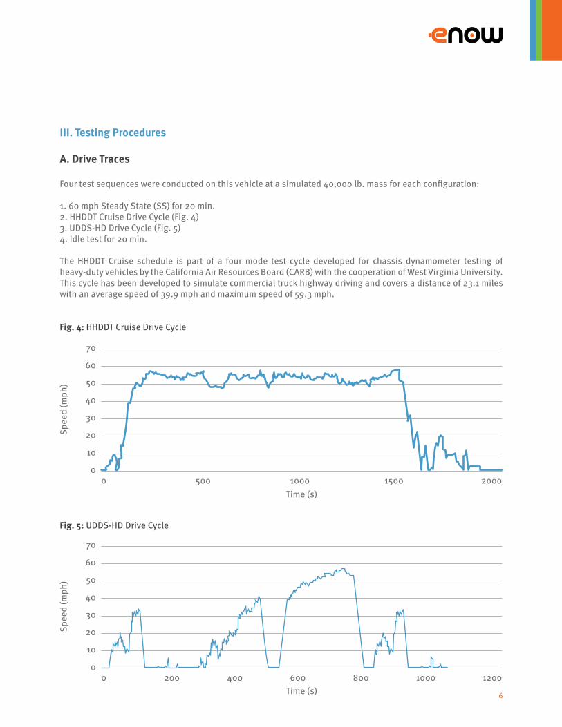
1. 60 mph Steady State (SS) for 20 min.2. HHDDT Cruise Drive Cycle (Fig. 4)3. UDDS-HD Drive Cycle (Fig. 5)4. Idle test for 20 min.
The HHDDT Cruise schedule is part of a four mode test cycle developed for chassis dynamometer testing of heavy-duty vehicles by the California Air Resources Board (CARB) with the cooperation of West Virginia University. This cycle has been developed to simulate commercial truck highway driving and covers a distance of 23.1 miles with an average speed of 39.9 mph and maximum speed of 59.3 mph.
Fig. 4: HHDDT Cruise Drive Cycle
Fig. 5: UDDS-HD Drive Cycle
6
70
60
50
40
30
20
10
0
70
60
50
40
30
20
10
0
0
0
500
200
1000
400
1500
600 800 1000
2000
1200
Spee
d (m
ph)
Spee
d (m
ph)
Time (s)
Time (s)
The UDDS-HD schedule was developed for chassis dynamometer testing of heavy-duty vehicles by the US EPA. This cycle has been developed to simulate commercial truck urban driving and covers a distance of 5.55 miles with an average speed of 18.8 mph and maximum speed of 58 mph. Both the HHDDT-Cruise and the UDDS-HD are industry recognized drive cycles representative of the operation of a Class 8 heavy duty vehicle.
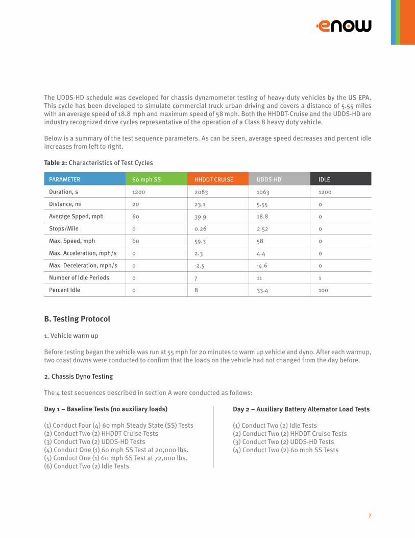
Below is a summary of the test sequence parameters. As can be seen, average speed decreases and percent idle increases from left to right.
Table 2: Characteristics of Test Cycles
B. Testing Protocol
1. Vehicle warm up
Before testing began the vehicle was run at 55 mph for 20 minutes to warm up vehicle and dyno. After each warmup, two coast downs were conducted to confirm that the loads on the vehicle had not changed from the day before.
2. Chassis Dyno Testing
The 4 test sequences described in section A were conducted as follows:
Day 1 – Baseline Tests (no auxiliary loads)
(1) Conduct Four (4) 60 mph Steady State (SS) Tests(2) Conduct Two (2) HHDDT Cruise Tests(3) Conduct Two (2) UDDS-HD Tests(4) Conduct One (1) 60 mph SS Test at 20,000 lbs.(5) Conduct One (1) 60 mph SS Test at 72,000 lbs.(6) Conduct Two (2) Idle Tests
Day 2 – Auxiliary Battery Alternator Load Tests
(1) Conduct Two (2) Idle Tests(2) Conduct Two (2) HHDDT Cruise Tests(3) Conduct Two (2) UDDS-HD Tests(4) Conduct Two (2) 60 mph SS Tests
7
PARAMETER
Duration, s
Distance, mi
Average Spped, mph
Stops/Mile
Max. Speed, mph
Max. Acceleration, mph/s
Max. Deceleration, mph/s
Number of Idle Periods
Percent Idle
60 mph SS
1200
20
60
0
60
0
0
0
0
UDDS-HD
1063
5.55
18.8
2.52
58
4.4
-4.6
11
33.4
IDLE
1200
0
0
0
0
0
0
1
100
HHDDT CRUISE
2083
23.1
39.9
0.26
59.3
2.3
-2.5
7
8
After Day 2 of testing some modifications were made to the testing setup in order to improve repeatability and expedite testing. First, the engine cooling fan was adjusted to stay on all the time. It was noticed that depending on the ambient temperature, the fan cycled on and off at different times and this of course changes throughout the day. By keeping the fan on, it eliminates that variability. Second, the AV900 Programmable Load was installed to emulate the auxiliary batteries. This eliminated the need to discharge batteries after testing and permitted more consistent loading.
Day 3 – Baseline and Programmable Alternator Load Tests
(1) Conduct Two (2) Baseline 60 mph SS Tests(2) Conduct Two (2) 60 mph SS Tests with Programmable Load(3) Conduct Two (2) Baseline HHDDT Cruise Tests
At this point in Day 3, the AV900 stopped working properly so the AMREL 1.5 kW programmable load was installed.
Day 3 Cont. – Baseline and Programmable Alternator Load Tests
(1) Conduct One (1) Baseline HHDDT Cruise Test(2) Conduct Two (2) HHDDT Cruise Tests with Programmable Load(3) Conduct Three (3) Baseline UDDS-HD Tests(4) Conduct Two (2) UDDS-HD Tests with Programmable Load(5) Conduct One (1) Baseline UDDS-HD Test(6) Conduct One (1) UDDS-HD Test with Programmable Load(7) Conduct Two (2) Idle Tests with Programmable Load(8) Conduct Two (2) Baseline Idle Tests
It was determined at this point that the cab A/C was not functioning on the vehicle so it was sent back to Ryder to be repaired. It was repaired along with other maintenance and sent back.
Day 4 – A/C On and A/C On with Programmable Alternator Load Tests
(1) Conduct One (1) Baseline 60 mph SS Test(2) Conduct Two (2) 60 mph SS Tests with A/C On(3) Conduct Two (2) HHDDT Cruise Tests with A/C On(4) Conduct Two (2) UDDS-HD Tests with A/C On(5) Conduct One (1) 60 mph SS Test with A/C On(6) Conduct One (1) Baseline 60 mph SS Test(7) Conduct Two (2) Idle Tests with A/C On(8) Conduct Two (2) Idle Tests with A/C On and Programmable Load
Day 5 – A/C On with Programmable Alternator Load Tests (cont.)
CENTER FOR AUTOMOTIVE RESEARCH | 15(1) Conduct Two (2) 60 mph SS Tests with A/C on and Programmable Load
8

IV. Results
Some preliminary testing showed that charging a set of four auxiliary batteries at a State of Charge (S.O.C.) of 30% adds an additional 100 amp of load to the alternator. For sake of time and repeatability, a programmable DC load was placed in the system to simulate the battery charging for vehicle testing. This load is representative of what the alternator sees if eNow’s solar charging system was not installed on a vehicle. Two standard drive cycles, one 60 mph Steady State, and one Idle test was conducted on the vehicle with and without the load, essentially with and without eNow’s charging system. Fig. 6 shows the increase fuel consumption with a 100 amp load on the alternator. The 60 mph Steady State tests showed an increase of 1.4% in fuel consumption with the 100 Amp alternator load compared to the no alternator load (i.e., baseline) test. The HHDDT Cruise and UDDS-HD drive cycles both showed about 2.5% increase in fuel consumption with the 100 Amp load. The Idle test showed the highest fuel consumption increase at 15.7% increase in gallons per hour consumed over the baseline.
Fig. 6: Percent Fuel Consumption Increase with 100 amp Alternator Load
The 60 mph Steady State and HHDDT Cruise sequences are a good representation of the type of driving a Class 8 sleeper cab (like the one tested) is likely to experience. The UDDS-HD is an EPA approved cycle for heavy duty vehicles to simulate a combination of city and highway driving. This cycle is not just intended for Class 8 vehicles but also Class 4 and Class 6. The idle sequences are a good illustration of the fuel used for all delivery and over the road vehicles if they are operated in that manner for long periods of time.
One can see from the graph in Fig. 7 that the Baseline vehicle had the best fuel economy at 5.86 mpg. The Baseline data is representative of a vehicle with eNow’s solar charging system, the “100 + amp load” test is similar to charging a set of auxiliary batteries. A second comparison in Fig. 8 shows the effect of having the A/C on while operating the vehicle, a typical real world situation.
The loads on the alternator can be seen in Fig. 9. Obviously, the baseline had the least load on the alternator having less than 20 kW-hr of energy it supplied to the system where the highest was the 105 amp load on the alternator in which it supplied almost 100 kW-hr of energy to the system. The alternator load with the A/C On had much less load on the alternator but the decrease in fuel economy can be attributed to the A/C compressor coming on and taking power from the engine.
9
181614121086420
60 mph SS(gal/mile)
HHDDT- Cruise(gal/mile)
UDDS-HD(gal/mile)
Idle (gal/hr)
Incr
ease
d Fu
el C
onsu
mpt
ion
(%)
1.4 2.6 2.7
15.7

Fig. 7: Fuel Economy of Test Vehicle at 60 mph Steady State with A/C Off Based on 4 Minute Test Intervals (10 Total Tests)
Fig. 8: Fuel Economy of Test Vehicle at 60 mph Steady State with A/C On Based on 4 Minutes Test Intervals (10Total Tests)
Fig. 9: Alternator Load at 60 MPH Steady State Based on 4 Minute Test Intervals (10 Total Tests)
10
6.00
5.90
5.80
5.70
5.60
5.50
5.40
5.30
5.20
120.00
100.00
80.00
60.00
40.00
20.00
0.00
Fuel
Eco
nom
y (m
pg)
Ener
gy (k
W-h
r)
Baseline
Baseline
100 + amp Load
100 + amp Load AC_On/80 amp load
6.00
5.90
5.80
5.70
5.60
5.50
5.40
5.30
5.20
Fuel
Eco
nom
y (m
pg)
AC_On/80 amp loadAC_On
AC_On

In Table 3, the tabular data of the graphs found in Fig. 6 and Fig. 7 can be found. Also one can see percent difference in fuel economy compared to the baseline test.
Table 3: Fuel Economy and Loads of Vehicle at 60 mph Steady State Based on 4 Minute Test Intervals (8 Total Tests)
Fig. 10: Fuel Usage at Idle Based on 5 Minute Test Intervals (8 Total Tests)
Tests at idle showed a 15.7% increase of fuel usage (Fig. 9) with a 100 amp load versus the baseline which was the highest percentage difference of fuel comparisons. This makes sense because the engine is producing its lowest power at idle so the extra load on the alternator has the biggest impact at idle.
The HHDDT Cruise and UDDS-HD drive cycle tests were conducted only two or three times (See Table 3) so there was not enough tests conducted to achieve statistical significance. It did show a recordable improvement in the fuel economy and more tests would need to be conducted to achieve a more precise level of confidence. However,
11
Baseline
100 + amp Load
AC_On
AC_On/80 amp Load
Baseline
100 + amp Load
AC_On
AC_On/80 amp Load
% DIFF
-
1.36
4.48
5.36
ST. DEV.
0.06
0.04
0.08
0.08
ST. DEV.
0.75
1.13
1.01
6.20
AVERAGE
5.87
5.79
5.61
5.56
AVERAGE
18.94
98.71
35.51
93.40
FUEL ECONOMY (mpg)
ALTERNATOR LOAD (W-hr)
1.20
1.00
0.80
0.60
0.40
0.20
0.00
Fuel
Usa
ge (g
al/h
r)
Baseline 100 + amp Load

the results of the drive cycle tests are in line with the 60 mph Steady State and Idling test results which show greater fuel economy improvement with decreasing average speed and increasing percent idle.
Table 4 shows the alternator loads for the various accessories on the vehicle. Each accessory was turned on and measured individually and then at the end, a group of main accessories were measured to get an idea of the alternator load for the most commonly used accessories. From these results, we can see a typical alternator load for this Class 8 truck might range from 13 to 66 amps without auxiliary battery charging. These loads could also be powered by solar, making this an additional opportunity for fuel economy improvement.
Table 4: Accessory Loads on Alternator
12
ALT. CURRENT (amp)
12.9
14.8
18.9
22.8
33.2
13.5
12.1
13.5
41.9
40.2
14.6
Alt. Current (amp)
65.9
ACCESSORY
ALL OFF (BASELINE)
FLASHERS
PARKING LIGHTS
HEAD LIGHTS-LOW
HEAD LIGHTS- HIGH
RADIO
WIPERS
AC LOW
AC HIGH
FAN HIGH
ALL INTERIOR LIGHTS
COMBINATION
HEAD LIGHTS-HIGH
RADIO
WIPERS
AC HIGH

V. Conclusions
Vehicle testing simulating eNow’s solar charging system showed an improvement in fuel consumption when charging a simulated set of auxiliary batteries. The smallest improvement of 1.4% in gal/mile was seen at the 60 mph Steady State point and the maximum was 15.7% in gal/hour. The drive cycles also showed improvement, between 2.6% and 2.7% in gal/mile depending on the cycle. When the air conditioner was turned on to simulate closer real world experience, the fuel economy (mpg) decreased by 4-5% for the 60 mph Stead State test sequence. In the future, an electrified cab A/C could also be powered by solar, making this an additional opportunity for fuel economy improvement.
The testing was conducted to simulate the fuel economy differences between a regular Class 8 vehicle to charge a set of auxiliary batteries against using eNow’s solar charging system to recharge the auxiliary batteries. However, since the eNow system removes load from the alternator, this scenario could be extrapolated to other vehicles that would use an auxiliary battery system to drive accessories and the alternator to charge those batteries. The fuel economy is based on the horsepower needed to operate a vehicle at a particular point or cycle and the extra load on the engine to charge auxiliary batteries. The larger the load on the alternator, the lower the fuel economy. While the fuel economy for smaller classes of vehicles can be expected to be higher (on average), one would expect to see similar percent improvements in fuel economy for other classes of vehicles as was seen here for the Class 8 vehicle.
The results of the overall system testing show the measureable impact of electrical load on the engine alternator and fuel economy. Although the dynamics of a long haul trip versus a short haul, local delivery trip are different, the resultant fuel economy degradation is measurable and significant over the life of the truck.
VI. Annex
Table 5: Fuel Economy for Various Tests
13
BASELINE
5.83
5.90
5.87
6.18
6.08
6.13
4.71
4.53
4.72
4.65
AC ON
5.60
5.62
5.61
5.69
5.84
5.77
4.13
4.37
-
4.25
AC ON/80 AMP
5.53
5.61
5.57
-
-
-
-
-
-
-
100 + AMP LOCAL
5.78
5.79
5.79
5.91
6.03
5.97
4.49
4.37
4.64
4.50
60 MPH SS Tests (20 min.)
Test 1
Test 2
Average
HHDDT - CRUISE
Test 1
Test2
Average
UDDS-HD
Test 1
Test 2
Test 3
Average

Table 6: Fuel Economy and Alternator Load at 60 mph SS
14
0
30649
0.9862
54136
2.0818
0
35828
11.3488
24394
0.0135
4
28418
4.9939
5.79
265.90
17.73
51932
6.1038
5.88
277.50
18.50
4
33590
15.367
5.78
1525.20
101.68
22156
4.033
5.79
1469.50
97.97
8
26214
8.9938
5.85
279.70
18.65
49717
10.1065
5.82
288.50
19.23
8
31337
19.3855
5.75
1488.50
99.23
19907
8.0529
5.76
1484.40
98.96
12
23970
12.994
5.74
278.40
18.56
47542
14.11
5.93
280.70
18.71
12
29101
23.4044
5.79
1474.40
98.29
17696
12.0729
5.86
1475.30
98.35
16
21770
16.9951
5.86
278.20
18.55
45357
18.1138
5.90
303.90
20.26
16
26870
27.4238
5.80
1467.10
97.81
15437
16.0931
5.73
1475.20
98.35
20
19583
20.9968
5.89
298.90
19.93
43183
22.1179
5.93
290.00
19.33
20
24611
31.4433
5.73
1470.40
98.03
13200
20.1134
5.79
1476.90
98.46
TIME (MIN)
TIME (MIN)
BASELINE - 092214
60 mph SS - 1
Miles
mpg
Average Power (W)
Average Energy (W-hr)
60mph SS-2
Fuel Reading (g)
Miles
mpg
Average Power (W)
Average Energy (W-hr)
AV900_105_amp-092214
60 mph SS - 1
Fuel Reading (g)
Miles
mpg
Average Power (W)
Average Energy (W-hr)
60 mph SS - 2
Fuel Reading (g)
Miles
mpg
Average Power (W)
Average Energy (W-hr)
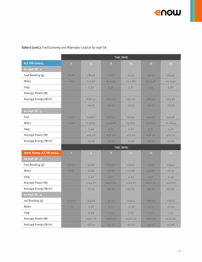
Table 6 (cont.): Fuel Economy and Alternator Load at 60 mph SS
15
0
28481
1.1862
53315
1.5561
0
33650
8.81
37902
1.30
4
28418
5.1196
5.52
608.30
40.55
50960
5.5705
5.49
495.70
33.05
4
31287
12.84
5.49
1140.70
76.05
35546
5.36
5.49
1470.10
98.01
8
23877
9.2139
5.72
602.20
40.55
48653
9.5918
5.62
475.50
31.70
8
28996
16.86
5.66
1440.60
96.04
33252
9.33
5.63
1436.40
95.76
12
21571
13.2287
5.61
592.60
39.51
46341
13.625
5.62
473.90
31.59
12
26621
20.88
5.45
1419.80
94.65
30954
13.36
5.65
1426.50
95.10
16
19241
17.2438
5.55
585.40
39.03
44026
17.6542
5.61
458.30
30.55
16
2430
24.89
5.58
1420.70
94.71
28639
17.39
5.61
1421.40
94.76
20
16930
21.2595
5.60
575.90
38.39
41778
21.6634
5.75
459.30
30.62
20
21942
28.91
5.49
1407.60
93.84
26566
20.94
5.51
1425.90
95.06
TIME (MIN)
TIME (MIN)
A/C ON-100214
60 mph SS - 2
Fuel Reading (g)
Miles
mpg
Average Power (W)
Average Energy (W-hr)
60 mph SS - 3
Fuel
Miles
mpg
Average Power (W)
Average Energy (W-hr)
Amrel_80amp_A/C ON-100314
60 mph SS - 2
Fuel Reading (g)
Miles
mpg
Average Power (W)
Average Energy (W-hr)
60 mph SS - 4
uel Reading (g)
Miles
mpg
Average Power (W)
Average Energy (W-hr)
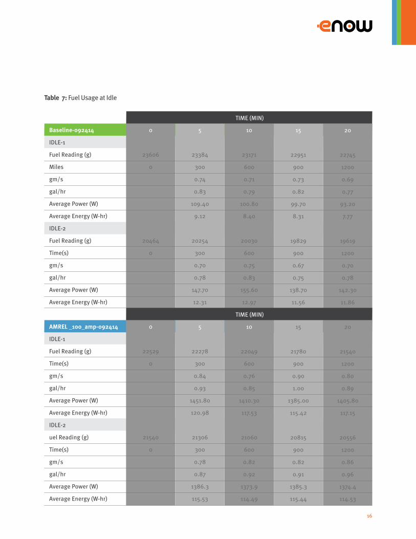
Table 7: Fuel Usage at Idle
16
0
23606
0
20464
0
0
22529
0
21540
0
5
23384
300
0.74
0.83
109.40
9.12
20254
300
0.70
0.78
147.70
12.31
5
22278
300
0.84
0.93
1451.80
120.98
21306
300
0.78
0.87
1386.3
115.53
10
23171
600
0.71
0.79
100.80
8.40
20030
600
0.75
0.83
155.60
12.97
10
22049
600
0.76
0.85
1410.30
117.53
21060
600
0.82
0.92
1373.9
114.49
15
22951
900
0.73
0.82
99.70
8.31
19829
900
0.67
0.75
138.70
11.56
15
21780
900
0.90
1.00
1385.00
115.42
20815
900
0.82
0.91
1385.3
115.44
20
22745
1200
0.69
0.77
93.20
7.77
19619
1200
0.70
0.78
142.30
11.86
20
21540
1200
0.80
0.89
1405.80
117.15
20556
1200
0.86
0.96
1374.4
114.53
TIME (MIN)
TIME (MIN)
Baseline-092414
IDLE-1
Fuel Reading (g)
Miles
gm/s
gal/hr
Average Power (W)
Average Energy (W-hr)
IDLE-2
Fuel Reading (g)
Time(s)
gm/s
gal/hr
Average Power (W)
Average Energy (W-hr)
AMREL _100_amp-092414
IDLE-1
Fuel Reading (g)
Time(s)
gm/s
gal/hr
Average Power (W)
Average Energy (W-hr)
IDLE-2
uel Reading (g)
Time(s)
gm/s
gal/hr
Average Power (W)
Average Energy (W-hr)
P O W E R I N G P O S S I B I L I T I E S
CENTER FOR AUTOMOTIVE RESEARCH930 Kinnear Road
Columbus, OH 43212
Phone: 614 292 5990
Fax: 614 688 4111
car.osu.edu
TECHNICAL CONTACTYale Jones
614 688 1138
BUSINESS CONTACTJames Durand
614 688 1137

P O W E R I N G P O S S I B I L I T I E S
CONTACT US TODAY TO LEARN MORE ENOWENERGY.COM
Rev. 9/17


