NASA Contractor Rep03 -3761 *s .I NASA CR 37fll- pt.1 c-1 Fully-Coupled Analysis of Jet Mixing Problems, Part I: Shock-Capturing Model, SCIPVIS Sanford M. Dash and David E. Wolf CONTRACT NASl-16535 JANUARY 1984 _- LOAN COPY: RETURN TO AFWL TECHNICAL LIBRARY KIRTLAND AFB, N.M. 87117
Transcript
NASA Contractor Rep03 -3761 *s .I
NASA CR 37fll- pt.1 c-1
Fully-Coupled Analysis of Jet Mixing Problems, Part I: Shock-Capturing Model, SCIPVIS
weak shear flow correction parameter for kE: model
static enthalpy
total enthalpy (= h + 3 Q2)
planar (J=O)/axisymmetric (J=l) flag
compressibility correction factor for ke model
turbulent kinetic energy
turbulent length scale
Mach number
turbulence Mach number
static pressure
production rate of turbulent kinetic energy
Prandtl number
total velocity
transverse distance
lower and upper jet boundaries
vi
RO T
U
u ’ i up. J V
W(4)
W
X
a
a. 1 5
17
E
Y
Y.. =J x'
P
u
af T 'I xr' xx' T rr 0
4
lJ
%
universal gas constant
static temperature
streamwise mean velocity
instantaneous velocity fluctuation
time-averaged components of Reynolds stress
transverse mean velocity
mixture molecular weight
turbulent vorticity
streamwise distance
subsonic (a=O)/supersonic (a=l)
mass fraction of ith species
mapped streamwise coordinate
mapped transverse coordinate
dissipation rate of turbulent kinetic energy
specific heat ratio
Kronecker delta
characteristic directions
gas mixture density
turbulent spread rate parameter
effective Prandtl number
laminar stress terms
flow angle (=tan-'V/U)
species mass fraction parameter
laminar viscosity
turbulent viscosity
ueff ;1
effective viscosity (=v+v~)
Mach angle
vii
1.0 INTRODUCTION
1.1 PROGRAM GOALS
This interim report describes computational methodology developed to analyze the plume flowfield generated by the interaction of an imperfectly expanded supersonic jet with the surrounding external stream. The overall goals of the present program are enumerated below.
(1) the development of a "fully-coupled" parabolized Navier- Stokes (PNS) computer code to predict the multiple-cell wave structure in a two-dimensional (planar or axisymmetric) turbulent jet exhausting into a quiescent or supersonic external stream;
(2) the formulation of techniques for the "strongly inter- active coupling" of the 2D jet solution with an external potential flow solution to provide for the,analysis of jets exhausting into subsonic/transonic external streams;
(3) the development of a fully-coupled PNS computer code to analyze the nearfield structure of three-dimensional turbulent jets (i.e., jets issuing from rectangular nozzles) exhausting into a quiescent or supersonic ex- ternal stream; and,
(4) the formulation of techniques for the strongly interactive coupling of the 3D jet solution with an external 3D potential flow solution.
This report discusses the accomplishments achieved in satisying the first goal listed above. Part II of this report describing accomplishments achieved in satisfying the second goal is now in preparation. The 3D methodology of the last two goals will be a direct extension of the 2D methodology. This 3D work is now in progress and will be documented in a forthcoming report.
1.2 APPLICATIONS
This effort is jointly supported by the Propulsion Aerodynamics and Aeroacoustics Branches of the NASA Langley Research Center, whose applications for this technology are quite disparate. The Propulsion
1
Branch is concerned with the influence of the jet exhaust on the nozzle afterbody pressure distribution for subsonic/transonic flight conditions. In a previous effort, Dash and coworkers developed an overlaid viscous/inviscid integrated by Wilmoth'
jet mode11T4 which was into a patched component nozzle afterbody
model. This methodology was demonstrated to work quite well in weakly interactive situations6'8, but, could not reliably treat strong viscous/inviscid interactions, and, was not readily ex- tendable to three-dimensional jet flowfield problems, In this program, new fully-coupled technology to deal with strongly in- teractive jet phenomena has been developedgs" which is readily extendable to 3D flow problems, as now being performed.
The Aeroacoustics Branch is concerned with the prediction of shock noise in imperfectly expanded jets. This requires a detailed portayal of the coupled multiple-cell wave/shock and turbulent mixing processes occuring in the jet (see references 11 - 13) which has not heretofore been available. The technology formulated in this program has led to the development of a new model and asso- ciated computer code14 which has been exhibitedI to provide this capability.
1.3 ACCOMPLISHMENTS
The accomplishments achieved to date in this program are summarized below.
(1) A 2D (planar/axisymmetric) PNS jet model (SCIPVIS)'4 has been developed which calculates the fully-coupled viscous/ inviscid jet interaction flowfield for a jet exhausting into a quiescent or supersonic external stream. A single- pass explicit spatial marching procedure is used to perform this calculation. SCIPVIS combines hyperbolic/ parabolic shock-capturing methodology for treating super- sonic portions of the jet with partially-parabolic methodology for treating subsonic portions. Compressibility corrected two-equation turbulence models are utilized to determine the local turbulent diffusivity, and specialized techniques are employed to locate Mach discs and calculate the interactive subsonic/supersonic mixing region downstream of the Mach discs.
(2) A series of ducted supersonic mixing calculations were performed to exhibit the ability of SCIPVIS to analyze fundamental interactive phenomenagal' (i.e., waves gen- erated by supersonic mixing and wave/shear layer inter- actions).
(3) A series of under and overexpanded free jet calculations were performed for jets exhausting into both quiescent and supersonic external streams to exhibit the performance of the SCIPVIS code under a broad range of operating conditions. The quiescent stream calculations were com- pared with the laboratory data of Seiner and Norum" in a code assessment effort performed by Seiner at NASA/LRC, which is documented in reference 15.
(4) A 2D partially-parabolic implicit model (SPLITP)' has been developed which calculates subsonic/transonic wall bounded and free mixing regions. The wall bounded version of SPLITP"r" was developed for David Taylor Naval Ship R&D Center to analyze curved wall jets over the aft portion of circulation control airfoils. For jet/afterbody inter- action applications, SPLITP is applied in the wall bounded mode over the nozzle afterbody and in the free jet mode, downstream. A direct coupling approach has been formulated for coupling SPLITP with an external potential flow solver which utilizes pressure-splitting methodology in non-reversed flow regions. A velocity-split coupling approach has been proposed for analyzing reversed flow regions. SPLITP pres- ently serves as a stand-along code for use in investigating jet/potential flow coupling techniques, A description of SPLITP and the coupling methodology developed will be pro- vided in Part II of this report.
An envisioned fina product of this technology for jet/afterbody applications would be a unified jet/boundary layer mode2 which combines the SCIPVIS and SPLITP models. The SPLITP portion would analyze the afterbody boundary layer and the subsonic portion of the jet mixing layer; the SCIPVIS portion would anaZyze the supersonic portion of the jet mixing layer. Direct pressure-6pZit coupling would be utilized in moderately interactive situations while velocity-split coupling would be employed in strongly interactive situations. This envisioned approach is conceptually the same for 2 or 3 dimensional problems.
This report (Part I) details the computational features of the SCIPVIS model and present results obtained for a spectrum of free and ducted problems, The SCIPVIS and SPLITP computer codes have been delivered to NASA/LRC and are operational at that facility. Separate documentation describes the operation of these codes. Part II of this report (Pressure-Split Model, SPLITP) describing the computational features of the SPLITP model and results for a number of free jet and wall jet problems is now in preparation,
2.0 OVERVIEW OF FULLY-COUPLED METHODOLOGY
2.1 JET FLOWFIELD CHARACTERISTICS
The analysis of the plume flowfield generated by the interaction of an imperfectly expanded jet with the surrounding external stream involves consideration of a number of distinct flow regions with varying characteristic features and length scales. Figure 1 exhibits the nearfield features of an underexpanded jet exhausting into:
(1) a quiescent external stream;
(2) a supersonic external stream; and,
(3) a subsonic external stream with a large boundary layer present.
In all these situations, the jet portion of the. nearfield is-charac- terized by a predominantly inviscid shock cell structure with mixing layers growing along the jet and Mach disc slipstreams. A transi- tional region (Figure 2) joins the predominantly inviscid nearfield with the fully viscous pressure-equilibrated farfield. Here, the mixing layers come to engulf the entire jet and wave processes occur in a fully turbulent environment. Wave processes are confined to supersonic regions of the flow bounded by the viscous sonic lines in the jet and/or Mach disc mixing layers (see Figure 1).
In the jet nearfield, strongly interactive phenomena occur in many situations which cannot adequately be anal zed using the earlier patched component (overlaid) methodology" 9 . Such interactive phenomena include:
(1) compression waves produced by the positive displacement effect of chemistry or high Mach number viscous dissipation in the jet mixing layer;
(2) expansion waves generated by the "washing away" of large mass defect initial regions downstream of base/separated flow zones;
4
l . ‘a.. ENTRAINED
‘...STREAMLINE . . A.,
/- JET MIXING LAYER
-.. SONIC LINE - M<l
ACH DISC MIXItiG LAYER
------ --- k- FIRST SHOCK CELL --
l QUIESCENT EXTERNAL STREAM
PLUME BOW SHOCK
/ PLUME MIXING LAYER
/ MACH DISC \ MACH DISC
MIXING LAYER
l SUPERSONIC EXTERNAL STREAM
b
First inviscid cell
l SUBSONIC EXTERNAL STREAM
FIGURE 1
Schematic of Jet Nearfield Structure for Quiescent, Supersonic and Subsonic External Flows.
--NEARFIELD--TRANSITION REGION 4-z FARFIELO -
l DAMPING OF WAVE AMPLITUDES
m: I -X
FIGURE 2
Schematic of Jet Nearfield, Farfield and Transitional Region; Damping of Wave Amplitudes by Turbulence in Transitional Region,
(3) the negative displacement of streamlines downstream of Mach discs (see Figure 1) generated by the wave-like entrainment process occurring; and,
(4) shock/shear layer interactions occurring at the end of shock cells for situations where a significant portion of the nearfield jet core has been entrained into the jet layer.
The above interactive phenomena are schematized in Figure 3.
The transitional region (Figure 2) where wave processes are large- ly embedded in the turbulent mixing layer, is always a region of strong viscous/inviscid interactions and cannot be treated by weakly interactive patched component technology, Here, wave intensities are damped by turbulent dissipation and wave fronts are curved by the higher mixing layer rotationality as exhibited in Figure 2. For many engineering applications (i.e., plume sig- nature predictions or plume/afterbody interaction problems), the
6
l SOURCE - LIKE DISPLACEMENT - PRODUCED BY TURBULENT DISSIPATION AND /OR COMBUSTION
. SINK-LIKE DISPLACEMENT -PRODUCED BY MIXING DOWNSTREAM .I REGIONS WITH MASS DEFECT
OF
l CURVATURE OF WAVES IN TRAVERSING ACROSS MIXING LAYER
nit Line
M, >I ------ --------
l WAVE/SHEAR LAYER INTERACTION - TRANSMISSION, REFLECTION, DISPERSION
FIGURE 3
Fundamental Interactive Phenomena Occurring in Supersonic Mixing Flowfields.
decaying wave structure in the transitional region has a negligible influence and can be approximated. For the analysis of jet laboratory data or for applications to problem areas such as jet shock noise11"3, the details of the shock structure in the trans- itional region are quite important.
The above interactive phenomena are all "quasi-parabolic" in the sense that diffusive processes along streamlines can be neglected. This report discusses several quasi-parabolic techniques developed to analyze such phenomena via the solution of a fully-coupled parabolized system of viscous/inviscid equations and the use of "direct-coupling" techniques to join together the various regions of the plume. The analysis of plume induced separated flow regions requires the use of fully-elliptic viscous/inviscid methodology which has not been formulated in this effort. An extension of the quasi-parabolic methodology using velocity-split coupling techniques can perform this type of analysis in significantly less time than full Navier-Stokes methodology and is now under investigation at NASA/LRC. An overview of the extensions required will be provided in Part II of this report.
2.2 BASIC MODELING REQUIREMENTS
The prediction of interactive jet flowfields entails the unification of modeling techniques for analyzing the following processes:
(1) wave/shock propogation in both inviscid and viscous supersonic regions of the jet;
(2) turbulent mixing in the nearfield jet shear layer (Figure 1) and in the transitional region (Figure 2);
(3) the influence of compressibility effects and pressure gradients on the turbulence;
(4) the strong interaction of the wave and turbulent structure as occur at the end of shock cells and throughout the transitional region;
(5) the interactive coupling of the viscous/inviscid jet with a subsonic or supersonic external stream;
8
(6) the occurrence of Mach discs and the strong interactions induced by the wake-like turbulent mixing process occurr- ing behind the disc; and,
(7) subsonic/supersonic coupling at the viscous sonic lines occurring in the jet and Mach disc mixing layers (Figure 1).
2.3 ANALYSIS OF WAVE/SHOCK PROCESSES IN SUPERSONIC INVISCID AND VISCOUS REGIONS
The treatment of wave/shock processes in inviscid flow regions is performed utilizipgg the SCIPPY model shock-capturing approach of Dash and Thorpele . Here, the equations are cast in conservative form and integrated utilizing the alternating one-sided difference algorithm of MacCormack" which permits embedded shock waves to be "numerically captured". This approach has yielded results equiva- lent to those obtained utilizing more cumbersome shock-fitting algorithms for a variety of jet exhaust flowfield problems (see Reference 19).
The extension of this shock-capturing approach to supersonic viscous flow regions involves the addition of parabolized stress/transport terms which render the resulting viscous/inviscid jet equations hyperbolic/parabolic. The use of a fully-coupled system of viscous/ inviscid equations to analyze wave processes in mixing regions was first introduced by Ferri in the mid-sixties for application to supersonic combustion problems (see the review article by Ferri*' for details of this earlier work). The numerical solution of these original fully-coupled equations employed a "viscous-characteristic" procedure** and a wide spectrum of problem areas were treated utilizing this technology. In present applications, the fully- coupled equations are termed the parabolized Navier-Stokes (PNS) equations and a number of numerical algorithms have been developed for their solution (see the review article of Dash and Wolf'). The shock-capturing algorithm utilized in the SCIPVIS model is described in detail in this paper. The ability of this shock-capturing algo- rithm to analyze basic interactive phenomena occurring in supersonic mixing regions" (i.e., the interaction of expansion fans and shock waves with shear layers, waves generated by high Mach turbulent dissipative processes, etc.) is demonstrated by numerical studies of ducted mixing. Complete jet flowfield solutions for supersonic jets exhausting into supersonic streams, predicted using this shock- capturing methodology, will be discussed. These studies have delin- eated conditions under which weakly interactive overlaid viscous/ inviscid coupling3 becomes inapplicable and fully-coupled methodology is required.
9
2.4 ANALYSIS OF QUASI-PARABOLIC SUBSONIC VISCOUS REGIONS
2.4.1 Embedded and Adjoining Subsonic Regions
In the interactive supersonic jet problem, we encounter both embed- ded and adjoining regions of subsonic quasi-parabolic viscous flow. Defining the jet portion of the flowfield to be that portion of the overall interactive flowfield bounded by the jet axis and the outer edge of the jet mixing layer (see Figure 1), two types of embedded subsonic regions occur, namely:
(1) the region behind Mach discs (Figure 1); and,
(2) the initial boundary layer dominated region of the jet mixing layer for jets exhausting into a supersonic stream (see Figure 2 - sinklike displacement schematic).
Adjoining subsonic viscous regions occur for supersonic jets ex- hausting into quiescent or subsonic/transonic external streams and occupy the region of the jet bounded by the jet mixing layer sonic line and the mixing layer outer edge (see Figure 1).
2.4.2 Pressure-Splitting Approximation
The governing flowfield equations in these subsonic regions are the same fully-coupled PNS equations used to analyze supersonic viscous flow regions. However, due to the elliptic character of the flow, a different numerical approach is required to integrate these equations. The approach taken here permits spatial marching in sub- sonic regions via the splitting of the pressure field such that the streamwise pressure gradient is "stipulated" while the crossflow pressure variation is arrived at via the coupled solution of the continuity and normal momentum equations. This type of approach has been implemented for both ducted and free jet mixing6problems by Spalding and coworkers23,24, Briley and McDonald2'p , and a number of other investigators.
Different types of splitting approximations are used to deal with the different subsonic flow regions, Downstream of Mach discs, the streamwise pressure gradient is suppressed in a manner akin to that implemented in supersonic external flow PNS solutions in the near- wall region*' (i.e., a "sublayer" approximation is utilized).
10
This approximation presumes that the Mach disc radius is small and hence, the acceleration of the subsonic flow behind the disc to supersonic velocities is dominated by the turbulent mixing process. The transverse pressure variation across the Mach disc mixing region is neglected under these circumstances. In analyzing the subsonic portion of the jet mixing layer for a quiescent external stream, the streamwise pressure gradient is set to zero; for sub- sonic/transonic external streams, it is set equal to the pressure gradient existing at the outer mixing layer edge as established by a potential flow solution.
2.4.3 Direct-Coupling of Jet and Potential Flow Solutions
The jet and potential flow solutions are "directly-coupled" at the outer edge of the jet mixing layer utilizing an approach that para- llels that of Bradshaw and coworkers2B*2g developed for boundary layer/potential flow coupling. Implementation of this approach has involved:
(1)
(2)
(3)
(4)
(5)
solution of the jet equations in a coordinate system which maps the outer edge of the jet mixing layer to a constant in mapped coordinates;
prediction of the jet boundary variation via an ordinary differential equation which accounts for both jet en- trainment and plume expansion;
solution of the subsonic jet equations using pressure- split methodology with the streamwise pressure gradient stipulated along the jet outer boundary;
revision of the streamwise pressure gradient via solution of the potential flow equations over a geometric surface comprised of the jet boundary with a transpiration boundary condition corresponding to the entrainment (radial) velocity component at that position; and,
the use of a "global" pressure update procedure2*'2g involving several sweeps of Step (3) for a fixed outer streamwise gradient to analyze regions with significant streamwise and/or normal pressure variations.
11
Steps (1) - (3) are operational in both the SCIPVIS and SPLITP computer codes. Steps (4) and (5) are under development using SPLITP. The details entailed in performing th,e above operations will be provided in Part II of this report.
2.4.4 Subsonic/Supersonic Coupling
In analyzing mixed subsonic/supersonic viscous flows, a formal coupling procedure is required to join the two solutions smoothly at the viscous sonic lines in the jet and Mach disc mixing layers (see Figure 1). Ferri and Dash22
The approach employed parallels that developed by to couple the subsonic and supersonic portions of
an interactive supersonic boundary layer solution. In this approach:
(1) convective and diffusive derivatives at the matching grid point smoothly connect variables on either side; and,
(2) a "viscous-characteristic" compatibility relation on the supersonic flow side ensures compatibility between the pressure and flow angle at the matching point.
In situations where normal pressure variations across the subsonic viscous layer are analyzed, and/or where the streamwise pressure variation is locally determined via an integrated continuity con- straint (as in analyzing the Mach disc mixing region), this coupling procedure is iterative.
2.5 TURBULENCE MODELING CONCEPTS
Turbulent mixing processes are represented using classical Boussinesq type approximations to relate the turbulent shear stress and scalar transport terms to the mean flow gradients. The turbulent diffusivity is determined using conventional models of the two-equation class which solve partial differential equations for the variation of the turbulent kinetic energy and a length scale parameter. This level of turbulence modeling represents the present state-of-the-art for "practical" analyses of high Reynolds number jet flowfields". Ap- plications to a complete spectrum of simple (constant pressure) free jet problems" had indicated that basic two-equation turbulence models performed reliably for low speed jet problems but performed poorly in supersonic mixing situations. Present generation two- equation models are all formulated from an incompressible viewpoint
12
and thus, their inability to deal with such compressible phenomena is not surprising. Extensions of two-equation models to deal with compressibility effects have thus far been heuristically formulated (i.e., no attempt has yet been made to formally model the terms embodying the compressibility effects of high Mach numbers). A detailed assessment of the performance of compressibility modified two-equation turbulence models for both simple and complex (variable pressure, chemically reacting) jet flowfields is given in reference 30. An overview of high Mach number compressibility effects on turbulent mixing and the specific "compressibility corrected" tur- bulence models employed in this effort will be discussed in this report. No attempt has been made to model the large scale structure of the turbulence 32 associated with the acoustic excitation of jet instability modes.
13
3.0 GOVERNING EQUATIONS
3.1 REYNOLDS DECOMPOSED JET MIXING EQUATIONS
The time-averaged, Reynolds decomposed, planar (J=O) or axi- symmetric (J=l) parabolized jet mixing equations33 are listed below.
Continuity
& burJ) + & (pVrJ) = 0 (1)
Streamwise (Axial) Momentum
& ([pt PU’] rJ)+ $F bUVrJ) = & (” Lx, - pm]) (2)
Normal (Radial) Momentum
& (pVrJ) t $([P+pV2]rJ)= 6 (il[ryr-pW])
Energy
& (pUHrJ) + -& (pVHrJ) = &- t $ - i$
I>
- PH'v' t hxr t TIXr) (U t u') t (Trr t Tlrr) (V t v')
Species Continuity
& (pU@rJ) + & (pVc#rJ) = $ rJ
0
t $f - pw I)
(3)
(4)
14
I - --- ,
These equations have been parabolized with respect to the axial (x) direction (viz. all transport terms with axial derivatives have been deleted) and "standard" (incompressible) assumptions concerning the turbulence correlations have been invoked (viz., third and higher-order correlations, density correlations {p'u', p'H' and ~'4') etc. are neglected). The transport of heat and mass is taken to be the same (i.e., the Lewis number is taken to be unity) and thus only the laminar/turbulent Prandtl numbers appear in the energy and species transport equations. In the above equations, U and V are the axial and radial velocity com- ponents, p is the density, P is the pressure, p is the laminar viscosity, H is the total enthalpy, and $ is the species para- meter.
3.2 THERMODYNAMICS
The jet mixing problems considered assume that the jet and external streams are each of uniform composition. For nonreacting (chem- ically frozen) situations, the species parameter 4 describes the local mixture composition; viz.,
a. _ a.
@ a1 a lE =
is iE (6)
where ai is the mass fraction of the ith species and J and E rep- resent the constant values of ai in the unmixed jet and external streams. The static enthalpy is given by:
W@,T) = ChJ(T) - hE( + hE(T) (7 1
where:
hJ,E i = C Caihi(T)lJ E #
Then the specific heat ratio, y($,T) is given by:
Y($,T) = Cp(~,VW)/Ro CpOb,VW)&-l (8)
15
where the specific heat, C P'
is given by:
Cp(h’V = g
and the molecular weight, W, is given by:
I -1
3.3 PARABOLIZED STRESS TERMS
Eliminating all terms containing streamwise derivatives, the laminar stress terms -rXr, ~~~ and 'err are as follows:
T au
xr = u'ar
T 2 av xx = - -pm
3 ar
T = 4 av rr 3%F
Using the Boussinesq-type approximation:
- PUi’U’. = 3
- ;pkSij + pt [(q + 2) - $ div v]
(where the turbulent kinetic energy k = ui'ui'/2), the para- bolized turbulent stress terms are as follows:
- pu’v’ = vtg
- pu’u’c 2 av - ;pk - TJI+E
- pv’v’c 4 av - ;pk + ptar
(9)
(10)
(12)
(1W
(13b)
(13c)
16
The turbulent transport of scalar variables, a, is expressed by.:
% aa -paT=,- a ar
(14)
where u or @.
a represents the turbulent Prandtl number, Prt, for a = H
3.4 TWO EQUATION TURBULENCE MODELS
In the generalized Prandtl-Kolmogoroff turbulence formulation (see, e.g., reference 34) the turbulent viscosity, pt, is related to the turbulent kinetic energy, k, and turbulent length scale, R, via:
% = C,,pk% (15)
where CV is a dimensionless constant. A partial differential equation can be formally derived to describe the production, dis- sipation, and transport of turbulent kinetic energy. By analogyj4, an equation can be formulated for the length scale parameter, z, which is related to k and R by:
z = kmQn
Table 1 shows three different popular forms of the length scale equation.
Table 1 - Forms of the Length Scale Equation
Model Z m n lJt/CpP
kc (Launder, et al.)Q E 312 -1 k2/c
kW (Spalding)b W 1 -2 k/W*
kw (Saffman)C w l/2 -1 k/w
aSee Reference 31
'See Reference 35
=See Reference 36
17
I
Only the ke" and kWSS two equation models have been incorporated in SCIPVIS and SPLITP. The kw model of Saffman36 (in particular, the modified version which accounts for compressibility") does show promise, as demonstrated by Walker" in his evaluation against Mach 2.2 jet data. However, this model has not been assessed against a singificant body of compressible jet data.
3.4.1 kc Turbulence Models
The kc models31 incorporated in SCIPVIS and SPLITP (ksl and ke2) are extended forms of the basic model which contain both axisym- metric and weak shear flow "corrections." The following equations are solved for k and E:
& (pukrJ> + R$ (.pvkrJ) =
& (pUcrJ) + & (pVsrJ) =
+ rJ (C1p - C2PE) t
In the above equations, g is
2 2 = lJt($
The turbulent viscosity, Ut, of k and E via the relation
% k2 = C,(Lz>P~
+ iJ (c - PE) (17)
(18)
the turbulent production term:
(19)
is determined from the local values
The following model constants" are utilized:
I kc1 I ks2
1.0 1.0
uE 1.3 1.3
c2 1.92 - .0667? 1.94 - .1336; I
I I C F! .09 - .04T I .09g(yE) - .05341 I
(20)
18
The axisymmetric correction parameter, ?, is set equal to zero in the shear layer region (before the mixing zone reaches the axis), and is defined bs
g = [2(ug Ue) (I2 I - i?)]“” (21)
downstream of that point (r is the width of the full mixing layer, UC is the jet centerline vefocity and Ue is the external stream velocity). The weak shear flow correction, g, is a function of the shear-stress weighted average ratio of production to dissipation rates. The functional form of g(P/c) is given in Figure 4.
FIGURE 4
-
Variation of g With P e For kc2 Model 7 (from Launder, et al. ')
19
3.4.2 Compressibility Corrected Version of kc Models (ks,cc)
The performance of the ks models in analyzing su$Trsonic jet and ~ shear layer data has been shown to be quite poor . An effort was undertaken to correct this model in a heuristic fashionjg to account for the reduced mixing rates observed for higher Mach number jet mixing. The compressibility corrected viscosity is given by:
(22)
where K(M,) is the correction factor and M, is the characteristic Mach number of the turbulence (MT = =x/a, where kmax is the maximum value of k at each station and a is the local sound speed at the grid point where k is maximum). The functional form of K(MT), given in Figure 5, was determined by matching calculations to observed spread rates for isoenergetic, supersonic shear layers with one stream stationary4'. Figure 6 exhibits the per- formance of the kE2 and ke2,cc models in predicting this spread rate data; the ke2 model shows no variation with Mach number while the kE2,cc model duplicates the data (as per the'calibration of KC+)). Note that the compressibility correction term goes to unity as compressibility effects diminish and hence, the kc2 and ke2,cc models are equivalent in lower speed situations.
3.4.3 kW Turbulence Model
The kW mode13', although developed at about the same time as the kE model, has not been widely used due to complications in applying it to wall-bounded shear flows41. However, a new version of the kW mode142 with coefficients set by rocket plume data has been employed successfully by the Propellant and Rocket Motor Establish- ment (PERME) in Great Britain. Predictions by PERME simulating laboratory rocket plume experiments performed at AEDC43 were quite promising and the overall assessment of this model by Pergament" for a spectrum of jet mixing problems was favorable. Hence this model has been incorporated into SCIPVIS and SPLITP.
20
FIGURE 5
Compressibility Correction Factor for kE Turbulence Models (from Dash, et a1.3g)
40 t
b 5 30-
f E e E E 20 E
0 kC2,CC /--
Best fit of doto &/AH-
a 0d 9
0 --AH a-
kr2
I I 2 3
Mach number, M,
I J 4 s
FIGURE 6
Spread Rates for Isoenergetic Compressible 2-D Shear Layers; M2 = 0; Data Fit From Reference 40.
21
The following equations are solved for k and W:
J r 't & (pUkrJ) + & (pVkrJ) = $-r (- ak
dk ar)
+ rJ (p - pCdkW*)
rJ % & (pUWrJ) + & (pVWrJ) = .& (- aW
g,
wg - C2pkW3'2 a2u 2 k + c3 % (9) -1
The turbulent viscosity is given by
Pt = - $
(23)
(24)
(25)
and the following model constants42 are utilized
Uk = .86
(SE = .86
CD = .09
c1 = 1.48
C2 = .18
c3 = 3.5
Note that this model contains no axisymmetric or weak shear flow correction terms.
The system of mean flow and turbulence model equations are solved in weak conservation form in SCIPVIS utilizing the mapped coordinates 5 andngiven by the simple rectangular transformation.
22
II = (r-rL(x>>/(rU(x)-rL(x))
(26)
where rL and rU are the boundaries of the jet domain being solved. With this transformation, the equations can be expressed in the following vector form:
where:
aE+ aF b2 a -- a< xi = rJ an
c f = 1, U, V, H, 9, k(l), E, k(2), W 1 T
(I) designates kc model (2) designates kW model
ek (1)
eE -a---
ek (2)
eW
e
PU
aP + pU'
PUV
PUH
PU@
pUk(')
PUE ------a.
Pd2)
puw
;H=b
PV
Pm7
P + PV2
PVH
PV@
pVk(l)
PVE --e-e---
pVk(2)
Pm .
(27)
-aB
23
and
Gf =
0 (a-l) ap/ax
0
b2 a -- rJ ar
"ueff('H-1) & aH
0
(c,P - 'C-p:) E/k 2 .---------------
P- pCDkW'
C,WP - C2pkW+ k
where:
In the above equations, given by:
a and b are the transformation parameters
I aK,rl> = Cl-n>r;_l + rlr;/(ru - rL) I I
b(S) = l/b, - rL> (28)
and a is a flow indicator (a = 1 for supersonic flow regions a= 0 for subsonic flow regions). The variable ueff is the combined laminar and turbulent viscosity. In practive, ueff is set equal to the turbulent viscosity for high Reynolds number jets and the turbulent stress terms in the radial momentum equation are deleted. The analysis of lower Reynolds number jets would entail the use of a low Reynolds number turbulent model formulation. Low R, two- equation turbulence models have been developed for boundary layer problems to treat laminarization and the near wall region. Their ability to predict laminar to turbulent transition is questionable (generally, an empirical transition relation is incorporated and a spot of turbulence is artifically introduced) and the coefficients have not been calibrated for free jet mixing problems. Hence, while low Reynolds number jet problems can be analyzed, substantial work in extending present turbulence models formulations may be required.
24
3.6 VISCOUS CHARACTERISTIC EQUATIONS
Boundary points in supersonic flow regions and subsonic/supersonic matching points are analyzed in SCIPVIS using formal characteristic relations. In viscous regions, the transport terms are included in the characteristic relations as local source terms using a viscous-characteristic formulation22. Along a X' characteristic (Mach wave) given by:
(29)
the following pressure/flow deflection angle (0) compatibility relation applies:
sinii cosp dlnp + de P -Jsin8 FV sin; dx
Y r - -
vPM* 1 cos(e f t)
In the above relations, G is the hlach is the viscous source term given by:
FV = SQ
where:
COST a sQ=-- rJ u
2U rJ ar eff ar
aH ar
angle (sin; = l/M) and FV
J a r 'eff (0 H - 1)
+ar uH
and Q is the total flow velocity (Q = (U2+V2)3>.
(30)
(31)
C32a 1
c32m
4.0 NUMERICAL PROCEDURES IN SCIPVIS
4.1 INTEGRATION OPTIONS
SCIPVIS provides for the spatial integration of the conservative jet mixing equations described by equation (27) using four types of integration options whose features and areas of applicability are described below.
4.1.1 Parabolic (Constant Pressure Mixing) Option
This option can be utilized to analyze balanced pressure subsonic or supersonic jet mixing. In utilizing this option: the pressure parameter a in equation 27 is set equal to zero (which removes the pressure term from the streamwise momentum conservation variable, euX the normal momentum equation is eliminated; the streamwise pressure gradient term, aP/ax, in the Gf vector array is set equal to zero; and, a parabolic decode procedure (to be described below) is used to extract the mean flow variables, i? conservation variables, eU, eH, and ea.
U, H, and I$ from the In analyzing a balanced
pressure jet (Figure 7), the equations are mapped from the jet axis to the outer edge of the jet mixing layer, rU(x), along which the external flow conditions UE, HE, and I$ = 0 are prescribed.
W
T MAPPED OUTER
M. L. BOUNDARY /
SCIPVIS PARABOLIC (TURBULENT MIXING) MODE
FIGURE 7
Parabolic (Constant Pressure Mixing) Option of SCIPVIS for Analyzing Balanced Pressure Turbulent Jet Mixing.
26
The inner mixing layer boundary "floats" across the grid points until it reaches the axis. The parabolic boundary growth rate, dru/dx, is based on the outer edge gradients of streamwise velocity, U, and species parameter, 9. and is given by:
drU ----I dx VIS
+J (zc) U
(33)
where f represents U and $ (the maximum gradient is utilized) and a value of C w 1 places the computational boundary, rU, in close proximity with the physical mixing layer boundary. Increasing C yields a buffer region of nonturbulent flow between the physical mixing layer edge and rU but does not effect the calculation except for decreasing the grid resolution. This integration option is employed in the analysis of underexpanded jets exhausting into a quiescent stream for analyzing the subsonic portion of the jet mixing layer, as will be described below.
4.1.2 Partially Parabolic (Pressure-Split) Option
This is an extension of the above option to account for streamwise and/or normal pressure variations in. the subsonic portion of the jet mixing layer using a pressure-splitting approximation. Here, the above parabolic option is first exercised (in integrating the equations from x to x + Ax) with the streamwise pressure gradient term, ap/ax, imposed*. This yields the mean flow variables U, H, and 4 at x + Ax.
The pressure, density, and radial velocity variation across the mixing layer are then arrived at via the coupled integration of the continuity and normal momentum equations and the equation of state constraint listed below (for a perfect gas);
* The procedure for determining the imposed streamwise pressure gradient differs in accordance with the subsonic region being analyzed, as will be discussed. A detailed review of pressure- split methodology will be given in Part II of this report.
27
H=&$+; (U2 + V2) (34)
where H and U are known from the parabolic integration and thus, P, p, and V at each grid point are related in a nonlinear fashion. In the standard (constant pressure) parabolic mode, the continuity and above state relation are solved in a coupled fashion to yield the variation of radial velocity and density across the jet mixing layer. The details of the variable pressure crossflow integration will be given in Part II of this report which describes the numerical procedures in SPLITP. This option has been exercised and employed in SPLITP but has not been implemented in the SCIPVIS studies per- formed to date. The partially parabolic option is also implemented to analyze the subsonic turbulent mixing region behind Mach discs and will be described in a later section of this report.
4.1.3 Hyperbolic (Inviscid Supersonic) Option
This option can be utilized to predict the nearfield inviscid wave/ shock structure in the jet (as a standalone option, it reduces to the inviscid SCIPPY modelles'g), and is, of course, utilized to predict the inviscid core region of underexpanded jets. To predict the inviscid supersonic jet structure (Figure 8): the transport terms in equation (27) are set equal to zero; the turbulence,equa- tions are eliminated; and, the equations are integrated with the parameter a set equal to one (i.e., the pressure is included in the eU conservative variable). The inviscid jet equations are mapped from the axis to the jet interface, rU, defined by:
drU -I dx INV
= tan Bu (35)
In performing an inviscid jet calculation, the pressure along the interface, rU, would be prescribed for quiescent or subsonic external flow and determined by a concurrent external flow solution (or the use of pressure/flow deflection rules such as shock expan- sion theory) for supersonic external flows (see reference 19 for details). A supersonic decode procedure is used to extract the flow variables: U, V, P, H, 4, and p from the conservation vector, F.
28
JET INVISCID ?LIPSTREAM, r”(x)
SCIPVIS HYPERBOLIC (SUPERSONIC WAVE) MODE
FIGURE 8
Hyperbolic (Inviscid Supersonic) Option of SCIPVIS for Analyzing Inviscid Shock/Wave Structure in Underexpanded Jet.
This option is utilized to analyze supersonic viscous (turbulent) regions of the jet. It is a direct extension of -the hyperbolic option with the transport terms evaluated and the turbulence model equations integrated. A brief description of this numerical algo- rithm and its application to the analysis of basic supersonic interactive phenomena was provided in references 9, 10, and 14. Details will be provided in this report.
The application of the above integration options in SCIPVIS in analyzing supersonic underexpanded jets exhausting into a super- sonic or quiescent external stream will be discussed below.
4.2 ANALYSIS OF UNDEREXPANDED JET WITH SUPERSONIC .EXTERNAL STREAM
Referring to Figure 9, the analysis of this fully supersonic problem (in the absence of embedded subsonic zones) involves utilization of the hyperbolic and hyperbolic/parabolic integration options. This is accomplished utilizing the techniques summarized below.
29
rl I TRANSMITTED
JET INDUCED BOW SHOCK
,& REFLECTED WAVE
UNDEREXPANDED JET/SUPERSONIC EXTERNAL STREAM
FIGURE 9
Schematic of Mapped and Floating Boundaries Distinguishing Various Regions of Supersonic/Subsonic Jet Mixing Solution
(1) The equations are integrated in mapped rectangular coordi- nates utilizing the transformation of equation (26) with rL=O and rU(x) corresponding to the outer edge of the jet mixing layer.
(2) The variation of rU(x) is obtained by combining the viscous and inviscid growth formulations given by equations (33) and (35) as follows:
dr ~IVIS,INV = tan eu + 2
L (-f$)
U (36)
30
(%
(4)
The position of the inner mixing layer boundary which "floats".across the grid points in working its way down to the axis is monitored by inspection of the 9 profile at each integration step. The hyperbolic (inviscid) equations are integrated below this position while the hyperbolic/parabolic (viscous/inviscid) equations are integrated above this position (as simply accomplished by setting the turbulent viscosity to zero for all grid points below the "floating" inner mixing layer boundary*).
Referring to the insert in Figure 9, properties along the outer viscous/inviscid boundary, rU(x), are obtained via solving:
(a) inner viscous (X+VIS) and outer inviscid (X-INV) characteristic compatability relations for the pressure, Pu, and flow angle, 0~; and,
(b) isentropic streamline relations along the entrained streamline, XSL (i.e., H = HE, P/pY = const) to yield remaining flow properties.
In original application; yf the SCIPVIS model to underexpanded jets in a supersonic stream 9 a single mapping from the axis to the fitted jet induced bow shock (Figure 9) was utilized eliminating the characteristic jet boundary solution procedure of Step (4) above. This was found to be numerically inefficient for a number of reasons (to be discussed in the applications section of this report). In present applications, the bow shock layer region (between r-u(x) and the bow shock, rBS(X) in Figure 9 is analyzed utilizing a second mapped domain {here, n = (r - ru(x))/(rgS(x) - ru(x))} implementating the hyperbolic option to integrate the shock
* While the hyperbolic/parabolic system of equations could be inte- grated across the entire viscous/inviscid jet, the representation of turbulence properties in the inviscid core using a high Reynolds number, two-equation turbulence model can pose numerical problems since the parabolized turbulence equations are not representative of the turbulence processes occurring (i.e., the requisite terms needed to represent core turbulence, the production of turbulence behind shocks and subsequent dissipation, etc. are not included in the parabolized turbulence model). Hence, it is most expedi- tious to eliminate the solution of the turbulence model equations in nonmixing regions rather than to solve an inappropriate system of equations.
31
layer equations, or, this region is not analyzed and the external supersonic flow is represented via simple one-wave relations such as shock-expansion the,ory (see reference 19). If simple one-wave relations are utilized, the outer characteristic compatibility relation along X'INV is replaced by a pressure/flow deflection rule stating the specific relationship utilized.
4.3 ANALYSIS OF UNDEREXF'ANDED JET WITH QUIESCENT EXTERNAL STREAM
Referring to Figure 10, the analysis of this problem involves utili- zation of both the hyperbolic and hyperbolic/parabolic integration options required in the fully supersonic problem, plus the parabolic or partially-parabolic integration option to analyze the subsonic portion of the jet mixing layer. This is accomplished utilizing the techniques summarized below.
I* MATCHING POINT
UNDEREXPANDED JET/ QUIESCENT EXTERNAL STREAM
FIGURE 10
Schematic of Mapped and Floating Boundaries Distinguishing Various Regions of Supersonic/Quiescent Jet Mixing Solution.
32
(1)
(2)
(3)
(4)
(5)
The equations are integrated using the same mapping as in the fully supersonic situation described in the previous subsection.
The variation of the outer mixing layer boundary, rU(x), is obtained by combining the viscous growth rule with the flow deflection angle at the sonic line position (not the outer edge angle as in the supersonic flow case*), viz.,
drU --I dx VIS/INv = Ilane M=l + fL
CrU #) U
(37)
As in the fully supersonic case, the position of the "floating" inner mixing layer boundary is used to delin- eate between hyperbolic and hyperbolic/parabolic flow regions. The hyperbolic/parabolic integ.ration is per- formed in the region bounded by the inner mixing layer boundary and the jet mixing layer sonic line.
Above the sonic line, the equations are integrated using the parabolic option with the streamwise pressure gradient, ap/ax, set equal to zero. The position of the sonic line is monitored at each integration step and also "floats" through the grid points, ultimately reaching the jet axis in the farfield at which point all "steady" wave processes terminate.
Two options are available to represent the radial varia- tion of pressure and radial velocity across the subsonic portion of the mixing layer which work as follows.
* For quiescent external flow, the flow angle of the entrained streamline can approach -90° and does not represent the "effective" inviscid slipstream variation.
33
(a) Parabolic Option
The pressure variation across the subsonic region is neglected. This is a reasonable approximation for the quiescent problem at modest pressure ratios; it would be a poor approximation for the nearfield jet with a subsonic external flow and large boundary layer since the streamline curvature induced by the "washing away" of the mass defect region of the external boundary layer can be quite appreciable (see references 3 and 4). In the parabolic option, the external pressure is imposed at the subsonic/ supersonic matching point (see insert of Figure 10) yielding the flow deflection angle via the viscous characteristic compatability relation of equation 30. Flow properties U, H, and 9 at the matching point are determined from the parabolic solution. Upward integration of continuity with the state constraint of equation 34 yields the radial variation of V and p and thus yields the outer edge entrainment (radial) velocity, VE, which can be used to upgrade the solution in a subsequent .iteration as will be described below.
(b) Partially Parabolic Option
The pressure, P, is assumed at the sonic line yield- ing, the flow angle, 8, and flow properties as above. Upward integration of the normal momentum equation yields the radial variation of P. The process is iterated upon until the predicted edge pressure is equivalent to the imposed external pressure. The steps described here are exhibited in Figure 11.
In performing quiescent external stream calculations, imposition of the ambient pressure level along rU and the use of the boundary con- dition, UE = 0 is only a first approximation to the complete inter- active problem.* The entrainment velocity., VE(X) predicted in this first approximation accelerates the "nominally" quiescent external
* The condition UE = 0 cannot (and should not) be simulated numerically since this implies vertical (-900) angles for the entrained streamlines which is physically nonrealistic - a nominal value of UE/UJ N l/100 can be simulated and is used to approximate the quiescent state in the first approximation.
34
JET MIXING LAYER
FOR OUTER BOUNDARY
POTENTIAL - Vc(rl Pet x 1 IMPOSED FROM POTENTIAL
SOLVER
l SOLVE n Parabolic” EOUATIONS FOR I*<f~IMAX .WlTH dp/dx= dPe/dx
.GUESS PI* AT x+Ax
GIS - VI+
*INTEGRATE COUPLED CONTINUITY /N,M. FROM I* TO IMAX - Pe , Ve
l ITERATE TILL Fe = PC
t PNS SUBSONIC PNS SUBSONIC
SOLUTION SOLUTION
---I- PNS SUPERSONIC
SOLUTION PNS SUPERSONIC
SOLUTION
I
I x +Ax
FIGURE 11
Pressure-Split Analysis of Subsonic Portion of Jet Mixing Layer.
flow. The entrainment induced pressure (PE(x)) and streamwise velocity (UE(x)) variations (obtained via coupling the jet solution with a potential flow solver) are implemented as boundary condi- tions along rU for a subsequent jet solution. This jet/potential flow iterative coupling approach is analogous to that required for analyzing subsonic/transonic external streams. The iterative methodology now under development will be discussed in detail in Part II of this report since SPLITP is being used to explore various coupling procedures. Direct coupling of SCIPVIS with a potential flow solver can be accomodated by the present code but this capabil4ty has not yet been tested.
35
4.4 ANALYSIS OF MACH DISC MIXING REGIONS
Referring to Figure 12, the mixing process that occurs between the inner subsonic flow that has traversed the Mach disc and the outer supersonic flow, has strong wake-like characteristics (viz. outer to inner PU ratios exceed 10 and can exceed 50 for highly underexpanded exhausts). The entrainment process displaces the outer streamlines inward at a very rapid rate for the first few Mach disc radii producing strong interactive effects. A simple p of Dash and Wolf4's
rocedure based on the "porous-sting" approach 6 for the two-phase Mach disc problem has
been developed for treating this interactive mixing process. This simplified approach utilizes a pressure-split "sublayer approximation" to eliminate elliptic (saddle-point) behavior in the marching process. This approach is applicable for smaller radius discs where the extent of the embedded subsonic zone behind the disc is small in comparison to the jet width and for which the turbulent mixing process dominates the acceleration of the inner flow to the supersonic velocities. The results obtained are in qualitative accord with the experimental observa- tions of Back and Cuffe14'. The basic features of the Mach disc methodology incorporated in SCIPVIS are summarized below.
MACH DISC DIVIDING S. L.
T) MACH DISC MIXING MATCHING SURFACE 4
/ -- M>I
/ ./ /
SUPERSONIC PNS -
---_ d-
I -2-
4 -
MCI I 4
At) SUBSONIC PNS
FIGURE 12
Characteristic Features of Mach Disc Mixing Region and Subsonic/Supersonic Matching Surface.
36
4.4.1 Disc Location
A formal triple-point shock fitting calculation is performed at each candidate disc location'g and a disc is dropped when a "sting" triple-point criterion is satisfied (i.e., when the streamline traversing the triple-point is parallel to the axis; locations upstream yield positive angles and locations downstream yield negative angles). This yields reasonable disc locations for smaller discs but locations somewhat downstream of observed locations for discs whose radius exceeds twenty percent of the total jet width. If the sting criterion has not been satisfied by the time the downrunning shock reaches the jet axis, the shock is regularly reflected. In a number of situations, shock reflec- tion/disc-formation has been observed"," at a position where use of the standard triple-point analysis breaks down (i.e., where imposition of the normal shock pressure level at the triple- point leads to a detached shock solution for the reflected shock). In such situations, the disc is dropped at the observed location (which has generally corresponded to the point where the Mach number behind the reflected shock at the triple-point first becomes sonic) using an "off axis" regular reflection analysis. Several of the cases described in reference 15 encountered this type of reflection condition and future experiments are planned to reveal the details of the specific reflection mechanism occur- ring.
4.4.2 Inner/Outer Matching Boundary
In cases where a disc is dropped, a grid point, sitting several grid points above the viscous sonic line (Figure 12) serves as the matching point between the inner subsonic and outer supersonic flows. A specified matching Mach number (typically 1.1 to 1.5) delineates the grid point at which inner/outer matching is per- formed. The grid points above the matching point are integrated using the supersonic viscous (hyperbolic/parabolic) or inviscid (hyperbolic) option dependent upon the position of the upper Mach disc mixing layer boundary (ascertained by inspection of a "dummy" inert tracer species profile initially assigned the value of unity for flow traversing the disc and zero for all other points). The grid points below the matching point are integrated using a variant of the partially-parabolic option with the pressure split using a sublayer type approximation. The index of the matching point changes from step to step in accordance with the monitored spatial variation of the sonic line. When the sonic line reaches the jet axis, the supersonic equations are employed and the inner/ outer matching is no longer required.
37
_.-.
4.4.3 Inner/Outer Matching
The following steps are entailed in the inner/outer Mach disc matching:
(1) A value of the pressure gradient, aP/ax, at the matching point I = I*, is assumed.
(2) The pressure field is split with the streamwise pressure gradient term in the axial momentum equation damped in accordance with the following heuristic sublayer approxi- mation:
= 0 for MI < 1
and the pressure, itself, given by:
pI aP
= PI* + ax I* Ax ( >
(3W
(38b)
(38~)
(i.e., the pressure is uniform across the mixing region but the pressure gradient is variable in the transonic portion and completely suppressed in the subsonic region).
(3) The inner grid points are integrated using the partially- parabolic algorithm (to be described) yielding the normal velocity at the matching surface, V*, and hence the "inner" flow deflection angle, 0*.
(4) The "inner" value of 8* is compared with an "outer" value given by a down-running viscous-characteristic compati- bility relation (this is analogous to the sonic line
38
matching depicted in Figure 11 with the subsonic and supersonic regions inverted). Steps (2) - (4) are repeated varying the assumed pressure gradient until the inner and outer values of 8* agree to within a prescribed tolerance.
The treatment of larger discs entails accounting for elliptic upstream influence effects using iterative methodology in con- junction with a downstream saddle point type viscous throat constraint" analogous to the minimum area throat constraint utilized in the Abbett inviscid Mach disc approach4' incorporated in earlier inviscid versions of the SCIPPY mode12#1g. The streamwise iterative approach required to treat larger radius discs appears to be a straight-forward extension of the present small disc methodology.
4.5 GRID DISTRIBUTION
4.5.1 Radial Distribution of Grid Points/Embedded Fine Grid
Referring to Figure 13, the grid points I = 1, 2, . . . . IMAX are evenly distributed between the jet axis, r = 0, and the outer edge of the jet mixing layer, r = r-u(x). In the mapped S,n rectangular
INVlSCtD SHOCK- CAPTURING SOLUTION
‘) =I
PLUME MIXING LAYER
FIGURE 13
Mapped Grid Distribution with Embedded Fine Grid In Thin Shear Layer Region.
39
coordinate system, the transverse coordinate n varies from 0 to 1 across the jet with the grid spacing, An, given by An = l/(IMAX-1). To provide sufficient grid resolution.in the thin nearfield shear layer, a grid embedding option is available which subdivides the standard grid intervals, An, into a number of subintervals as exhibited in Figure 13.
Referring to Figure 14, the embedded fine grid region is initiated at, grid point 'f selected to fall one (coarse) grid interval below the interval containing the "f'loating" lower shear layer boundary, r&d. The ratio of fine grid (A:) to coarse grid (An) spacing is given by:
where n is initially user selected. The coarse grid points,
K = i + (IMx-:).2"
K= -i + 2.2"
K=1+2"
K= i
P--AC --i E
FIGURE 14
Details of Embedded Fine Grid.
40
I = I to IMAX, are reindexed in accordance with the relation:
K= i + (I - ;>*2n
with K varying from i to KMAX - i + (IMAX - 1)*2" as exhibited in Figure 14_for n = 2. The coarse grid integration for grid points I = 1 to I is performed first yielding propertigs at E + AC. The radial derivatives at the bounding grid point, I, are evaluated using the coarse grid interval, An, and the integration as per= formed in the inviscid limit. The interval between I = I and I + 1 serves as an inviscid buffer zone.
After the coarse grid integration, the fine grid insegration is performed from 5 to 5 + A5 for thg grid points K = I + 1 to KMAX utilizing a reduced axial step, A5 (chosen to be a fraction of the coarse grid step size, AC, in accordance with stability require- ments to be discussed below). Note that all properties along K = ? are known from the coarse grid integration and serve as lower boundary conditions for the fine grid integration. At the end of the combined fine/coarse grid integration step, the f&oating lower mixing layer edge_ is located and the matching point I is shifted if required. As I is moved down, the number of fine grid points increases as does the total number of overall grid points. The ratio of the shear layer width to the full jet width is maintained to be less than 1 2n
i (i.e., if n=3, the width of the shear layer should
not exceed th the overall plume width). If the shear layer width ratio exceeds the grid ratio, n is reduced by 1 which decreases the number of grid points in the shear layer by a factor of 2 (i.e., every other point is discarded). When the shear layer exceeds 4 the jet width, a single grid interval is used. An additional con- straint on n is the total number of gr_id points dimensioned, viz, n must-always be decreased if moving I down leads to the situation where I + KMAX > I* where I* is the maximum dimension of I in the variable arrays.
4.5.2 Axial Step-Size Criterion
The SCIPVIS algorithms are fully-explicit and thus, the allowable marching step, AE,is limited by both hyperbolic and parabolic stability constraints. The following step-size criterion are utilized in the various flow regions of the jet.
41
(a) Hyperbolic Stability Criterion
In inviscid supersonic flow regions, the step-size is limited by the well known CFL condition which requires the physical domain of dependence to fall within the numerical domain. This criterion is satisfied in a non-linear fashion by locating the intersection of the h+ characteristics with the mapped coordinate grid lines, n = const, at each grid point, I, and, deter- mining the minimum intersection for all grid points. At each grid point I, the maximum allowable step-size is given by the relation:
(39)
where 9 and u are the flow and Mach angles, and w is the mapped grid line angle given by:
tanwI = rL' + > (I:k-'l) 6J - y)
(b) Parabolic Stability Criterion
In viscous subsonic flow regions, the parabolic "diffusion equation" criterion is applied which requires that:
2 2 l 5pUuminb An
% (40)
(c) Hyperbolic/Parabolic Stability Criterion
In viscous supersonic flow regions, the hyperbolic and parabolic criterion are combined in the following fashion at each grid point I:
HYP/PAR (41)
42
This viscous/inviscid step-size was first utilized by Cheng" in the explicit integration of the time-dependent Navier-Stokes equations and had proven effective in earlier "viscous- characteristic" finite-difference analysis of supersonic mixing problems by Dash and coworkers (see, for example, Reference 51).
4.6 INTERIOR POINT INTEGRATION PROCEDURES
4.6.1 Generalized Finite-Difference Algorithm
The following "generalized" two-step algorithm is utilized in all regions of the jet flowfield to advance the solution of equation (27) from 5 to E + AC at grid point I, for equally space trans- verse grid intervals, An:
Predictor Step:
EI - EI (1-e) FI+l - (l-2e) FI - eFI,l - GI AC
Corrector Step:
where:
43
and e is an upwind/alternating one-sided convective difference parameter whose operation differs in different flow regions as will be described below. The diffusion terms are evaluated using a standard central difference operator in all flow regions.
4.6.2 Supersonic Marching Procedure
In supersonic viscous or inviscid flow regions, the convective difference parameter, e, in the above difference equations is varied between zero and one in the predictor and corrector steps to provide one-sided, alternating differences for shock- capturing. The resultant algorithm is the stea$g flow equivalent of the well known explicit MacCormack algorithm . The "e" sequence is alternated at subsequent marching steps to yield a nonpreferential treatment of wave propogation. The pressure parameter, OL, (see equation 27) is set equal to one in super- sonic flow regions, thus including the pressure term in the eU conservative array and eliminating it from the source term, G. A standard supersonic decode procedure'e,'g is used to obtain the variables, P, p, U, V, H, I$, k, E, from the conservation arrays at the end of the predictor and corrector steps.
4.6.3 Upwind Modification of Convective Operator for Scalar Variables
In a number of applications of the supersonic algorithm, oscilla- tory behavior of the scalar variables (H, 4, k and/or s) occurred in situations where the mapped grid was significantly skewed with respect to the streamline directions and radial gradients of the scalar variables were large. In parabolic problems, this unstable type of behavior is remedied by the use of an upwind convective operators2. To provide this remedy in a shock-capturing algorithm, the convective difference operator for the scalar components of the F vector array can be split into upwind and alternating one- sided difference components as follows:
aF* arl=a -& (PV> + PV g
aZte2wating upwind
(43)
where:
a = [H, +, k, EIT
44
and F* represents the scalar elements of the F vector array. With this splitting, the following convective difference expres- sions are utilized in the predictor and corrector steps:
Predictor Steu:
aF* 1 arl -xii "I
[ f (l-4 W)l+l - (l-24 (PW, - e(PW,-,
I
+ (PVIIK I
(l-e*) aI+ - (l-2e*) aI - e* aIml I
Corrector Sten:
r a%* 1 - - all =Tiy aI
L f
e(W) I+1 + (l-24 G), + (e-1) (P+I-l t
+ (iGl f e*GI+l + (l-2e*) GI + (e*-1) GIml
WW
(44b)
The parameter e is the standard alternating difference parameter, whereas e* is the upwind difference parameter defined (in both the predictor and corrector steps) by:
e* = 1 if V/U 2 a/b
e* = 0 if V/U < a/b
where a and b are the mapping parameters given by equation 28. For the continuity and momentum equations, the standard alternating- difference MacCormack algorithm is utilized with no splitting. The splitting of the scalar components of the F vector array has no effect on the shock-capturing characteristics of the algorithm (the scalar variables, a in Equation 43, all change continuously across shock-waves). Thus, the nonconservxve differencing of these variables in the vicinity of the captured shocks poses no problem.
45
This has provided a simple and reliab.le remedy to the oscillatory problems encountered. This approach is recommended as a general extension of the conservative MacCormack algorithm in both steady and unsteady flow applications, in regions where such oscillatory problems are anticipated. In use of the MacCormack algorithm with nonconservative flow variables, an analogous practice is the upwind solution of the entropy equation in entropy layer regions (see references 53 and 54).
4.6.4 Subsonic Marching Procedure
For grid points in subsonic regions, the pressure parameter, (Y, is set equal to zero and hence, the streamwise pressure gradient is included in the source term array, G, and does not appear in the conservation variable arrays E and F. The full system of conser- vation equations are integrated from 5 to 5 + A& using the two- step algorithm of equation 42 in the manner described below.
(1) Upwind convective differencing (utilizing e* defined by equation 45 in 44) is used for all variables in both the predictor and corrector steps, -
(2) The pressure field is split with the streamwise pressure gradient m (not BP/aE), imposed and the normal pressure gradient, aP/an, evaluated from the known profiles at x.(predictor) and x+Ax (corrector).
(3) Dependent variables U, V, H, 4, k and E are obtained via a simple subsonic decode procedure, viz.:
f = ef/ep (46)
where f represents the dependent variables and e P = pu.
(4) The pressure and density are evaluated from the relation:
WE+AS>, (47)
46
and the equation of state (listed here for a perfect gas):
-1
P(S+W, +(u2+v2) 1 (48) I
(5) The conservation variables, ef, are reconstructed in accordance with the value of p obtained from equation (48) and the decoded variables U, V, H, #I, k, E given by equation (46).
(6) After the predictor and corrector steps have been com- pleted, the dependent variables V, P and p are revised via a crossflow integration procedure with the variables U, H, I$, k and E: held fixed at the corrector values established in Step (3). The crossflow integration procedure utilizes the continuity and normal momentum equations, and the equation of state constraint, and en- tails the coupled solution of three nonlinear relations at each grid point. Procedures for solving these relations are described in detail in Part II of this report. The linearized procedure utilized in SCIPVIS in situations where the normal pressure variation across the subsonic is neglected is described in the next subsection.
(7) The conservation variables, ef, are upgraded in accord- ance with the revised values of p and V obtained in Step (6).
4.6.5 Subsonic Continuity Equation Integration
Let the.revised values of p and V at the grid point 1,K (point C of Figure 15) be given by:
P = P* + PC (490
v= v* + v’ l-b)
47
FIGURE 15
Grid Nomenclature for Subsonic Continuity Equation Integration.
where p* and V* designate the values determined via steps (1) to (4) of the previous subsection and p' and V' are corrections to these values to be determined by the linearized procedure discussed below. The mass flux at point C integrating upward from point A is given by:
* c % = JI, + AQAc + AQ~~
* where A@,, is the flux based upon the unrevised values, viz:
* '+A, = +bAuArAJ + Pc*ucrcJ)bKh
and A+ic is the linearized correction term given by:
(50)
. A’QAC = +P& JbKClri
48
The mass flux at point C integrating streamwise along BC is given by:
JIG = 9, + A$;, + A&
where AJIG, is based upon the unrevised values, viz:
* “JlBc = - +(PBrBJ + P$CJ)vgAg
+ $tPBUBrBJ + pzUCrCJ) $$ A< [ 1 BC
with the grid line inclination, dr/dx given by:
and the linearized correction term, A$&, given by:
* A$,, = - +(PBrBJ + P$-cJ)ViAc
(51)
Equating the values of JlC given by equations (50) and (51) yields the linear p', V' relation listed below:
c r AlPC + A2VC = & (A& - A& + $B - +A> (52)
49
where:
Al = rcJUc bKAn + [ ('>, - kd,,]
and:
A2 = PBrB J *J + pcrc
Replacing Vi in equation (52) with the linearized equation of state constraint given by:
yields:
* PC =
2 AUJ~C-A$~C+$B-~JA (Al+A2/A3)U
(53)
(54)
The subsonic continuity integration sweeps upward from the axis, for the Mach disc subsonic region, and from the jet sonic line, for the jet mixing layer subsonic region. Both integrations are initialized with pc = V' = 0.
It should be noted that the streamwise continuity relation given by equation (51) does not involve the V distribution at the pre- vious streamwise step Fis appropriate to parabolic situations55'56. This implies that the V distribution is evaluated at the midpoint of the integration step (i.e., 5 + A5/2), an assumption generally invoked in present generation parabolic algorithms. The use of the normal momentum equation to yield the provisional values of V in situations where the normal pressure variation is neglected serves as a "redundant" stabilizing factor in the overall algo- rithm and essentially implies that the normal velocity component is convected along the flow streamlines until corrected by the linearized continuity relations of this subsection. The basic
50
assumption is that the continuity induced V' correction to the value predicted by the normal momentum equation is small, which is generally the case except in the initial jet region, and in regions at the end of shock cells where the flow angle changes discontinuously in the vicinity.of the jet sonic line. In these regions, several iterations may be required accompanied by an underrelaxation process to stabilize the V" change from iteration to iteration.
4.7 BOUNDARY POINT PROCEDURES
The following boundary point procedures are incorporated in the SCIPVIS model:
The shock point and wall point calculations are performed in the inviscid limit* utilizing predictor/corrector characteristic based procedures which are described in detail in references 57 - 59. The remaining boundary point procedures will be described below.
* The shock point calculation is used to analyze the jet induced bow shock depicted in Figure 9; the wall point calculation is utilized in analyzing ducted mixing problems (to be described in Section 5) with the wall region treated in an inviscid fashion (i.e., the mixing region does not extend to the duct walls and wall boundary layer effects are neglected).
51
- _..-.-- --..
4.7.1 Axis Calculation
At the jet axis (or plane of symmetry), the conservation equations take the following limiting form:
g + (l+J)pi; g + Gf = ueff a27 (l+J) - - "f ar2
.
where:
(55)
3V -= bP2-Vl) ar Arl
and:
a27 = b2(T2-Fl)
ar2 AT12
where subscripts 1 and 2 denote the grid points at the-axis and_ one grid interval above the axis. The vector arrays, E, 7 and Gf are defined in Section 3.5. A two-step predictor/corrector pro- cedure is used to integrate equation (55) in both supersonic and subsonic regions (behind Mach discs) with the pressure parameter a set equal to 1 or 0 and the axial pressure gradient predicted or prescribed accordingly.
The supersonic axis solution procedure is modified beyond the position of the first reflected shock (orMach disc sonic line) to avoid oscillatory behavior at subsequent shock reflection points. The modification effectively reflects waves off of a sting whose radius corresponds to one grid interval. This eliminates the highly nonlinear axisymmetric wave strengthening that occurs in the vicinity of the axis that cannot be resolved using standard grid spacing. The modified axis procedure works as follows:
52
(1) The axial pressure gradient at grid point 2 is deter- mined utilizing a X- viscous-characteristic relation (see equation 30) with the flow deflection angle at point 2 set equal to zero (i.e., the flow is enforced to be parallel to the axis).
(2) The conservation equations at grid points 1 and 2 are solved with a = 0 imposing the axial pressure gradient determined from the X- relation of step (1) and neglecting the normal pressure variation between 1 and 2.
(3) The conservation variables at grid points 1 and 2 are decoded using the simple (pressure prescribed) decode relations of equation 46; V is set equal to zero at both grid points and the density is determined from the state relation (equation 34).
4.7.2 Jet Mixing Layer Outer Edge Calculation
For a supersonic external stream (Figure 9), properties along the outer edge boundary, rU(x), are determined using characteristic relations as exhibited in the insert of Figure 9 and summarized in Section 4.2. The calculation is analogous to a standard con- tact surface calculation (see references 19, 57 - 59) modified to account for jet entrainment across the boundary. The following sequence of operations is entailed in performing the supersonic outer edge calculation in marching from 5 to 5 + AC:
(1) The outer edge is locating utilizing equation 36, which takes the following difference form for I = IMAX:
Predictor:
rU = r,(S) +
Corrector:
r
I taneu(E) + Cr,(E)b(S> (fI-fI-l) f (Sja,, T I L
(560
(56b)
53
(2) The 'Ifeet" of the X+vIs, X-, and XSL characteristics (i.e., the intersection of these characteristics with the initial data line at E) are determined via com- bining the characteristic geometry relations given below with linear property variation relations along the initial data line. The characteristic geometry relations are given by:
Predictor:
2*(E) = Su + X*(E)AE
Corrector:
r*(S) = r,(c+AE) + i i*W+k+AE) A5 1
(570
(57b)
and are solved concurrently with interpolation relations for X* in both the predictor and corrector steps to yield a noniterative location procedure (see references 19 and 59 for details). In the above relations, A* represents X+, X' or Xsh where ;X designates the slope of the charact- eristic line (viz., X+ = tan(B+u); ASL = tang). Properties at the foot locations, r*(E), are obtained via linear interpolation. The viscous source terms in the X+vIs com- patability relation are evaluated via standard central difference relations at the grid points and interpolated at the foot location.
(3) The pressure, P, and flow deflection angle, 8, are eval- uated via the X+ and A- compatibility relations listed below.
predictor:
A+(F) Rn (G/p+) + e-e+ = B+(E>U
A-(E) Rn (g/P-) - i+e- = B-WAS
(5W
(58b)
54
. . ..-..._ -._
Corrector:
1 T ?(c)+?(c+Ac) 1 an(~/G+)- t&i- = + i-(E)+?(&+A&) 1 A& (59b) In the above relations,
A’ = sinu cosu Y
and:
B+ = -Jsine FV 1 sinu _ r yPM2 cos(e+d
In the predictor step, A' and B', and, the properties 8', Pf in equation (58) are evaluated at the "foot" points rf given by equation (57). In the corrector step, A* and B+ are averaged across the characteristic, and, the = nota- tion for the values at the 5 station indicates that these values have been updated in accordance with the shift in the characeristic foot position between the predictor and corrector steps. The same nomenclature applies to the up- dated values of 5' and F' at the 6 station.
(4) The total enthalpy and density are evaluated along the streamline y8I via the relations:
dH 0 -= dX
and:
55
(5) The species parameter, 0, the turbulent kinetic energy, k, and the turbulent parameters E or W are set equal to zero along the outer boundary.
(6) The velocity Q=(U2+V2)3 relation (eq:ation 34)
is determined from the state a;d the U and V components are
evaluated from the relations:
u= &cost3
v= Qsine
If the external flow is simply represented via the use of pressure/flow-deflection relations, equations 58b and 59b are replaced by these relations, and the entropy level is assumed constant in the external flow.
For subsonic or quiescent external flow (Figure lo), the axial pressure variation is prescribed along the outer jet boundary, rU(x 1, along with the axial velocity variation, VU(x). The total.enthalpy is taken to be constant and 4, k and E (or W) are all set to zero. The radial (entrainment) velocity variation, VE(x), is determined via integration of the continuity equation aposteriori, as described in Section 4.6.5. The coupling of the subsonic and supersonic portions of the jet at the viscous sonic line (Figure 10) entails the use of characteristic methodology as described below.
4.7.3 Subsonic/Supersonic Matching Point
Referring to the insert of Figure 10, subsonic/supersonic coup- ling at the matching point, I*, entails stipulation of the pressure at the matching point and determination of the flow angle, e*, via a A+ viscous characteristic relation. For the quiescent external flow problem in a mildly underexpanded situa- tion, the external pressure is imposed at the matching point. Use of the subsonic marching procedure described in Section 4.6.4 yields the dependent variables U, V, R, $I, k and e'at‘the match- ing point. The normal velocity, V, is then revised in accordance with the relation:
V* = U tane*
56
and the density, o*, is determined from the state relation. The subsonic continuity integration procedure (Section 4.6.5) is initiated at the I* point and works upward to the jet outer edge.
For subsonic external flow, the pressure at the matching point is assumed but the axial pressure gradient at the outer edge (aP/ax)U, is imposed in performing the subsonic marching procedure along I* (viz., the pressure field is split in the standard fashion). In the first iteration, the pressure at the matching point, P*, is taken to be given by:
P*(.$+AE) =
The iteration proceeds until the pressure at the jet outer edge determined from the coupled solution of the continuity and normal momentum equations agrees with the prescribed outer edge pressure. This iterative methodology has been schematized in Figure 11.
An analogous procedure is performed at the subsonic/supersonic matching point in the Mach disc mixing layer (Figure 12). The pressure splitting differs here since the upstream influence effects can produce departure solutions unless the axial pressure gradient is supressed using a sublayer type approximation. In the jet mixing layer, the upstream influence effect is already incorporated via stipulation of the axial pressure gradient in accordance with an external potential flow solution arrived at apriori. The details of the Mach disc matching point solution have been provided in Section 4.4.2.
4.8 INITIALIZATION PROCEDURE
The initialization procedure utilized is directly analogous to that employed in the previous overlaid viscous/inviscid jet models', . The initialization entails:
(1) determining the initial jet inclination angle in the inviscid limit to achieve balanced pressure across the jet slipstream (see references 18 and 59 for details);
57
(2) determining initial mean flow shear layer profiles centered about the jet slipstream location a small distance downstream of the nozzle exit plane (see references 1 and 2 for details); and,
(3) determining initial turbulence parameter (k and E or k and W) profiles based on an equilibrium tur- bulence hypothesis and the use of a mixing length turbulence model approximation (see references 1, 2 and 30 for details).
58
5.0 APPLICATIONS OF SCIPVIS MODEL
5.1 WAVE/SHEAR LAYER INTERACTIONS
To illustrate some of the fundamental interactive phenomena that can occur in the nearfield jet shear layer, a series of calcula- tions were performed for a supersonic shear layer in a duct. The wall region of the duct was treated inviscidly and the duct wall was turned to generate shock and expansion waves. All calculations were performed using the kc1 turbulence model and employed thirty grid points equally spaced between the duct walls.
SUPERSONIC/SUPERSONIC SHEAR LAYER 0 nl Y j, I
A 8 C z
FIGURE 16
Predicted Wave Pattern Induced by Supersonic Shear Layer in a Parallel Wall Duct.
5.1.1 Waves Generated by Supersonic Shear Layer
In the first calculation, the duct walls remained parallel. Ex- hibited in Figure 16 are the perturbation pressure waves'produced by the mixing of uniform Mach 2.4 and Mach 4.8 streams, both initially at T = 1000 OK and P = 1 atm. Figure 17 depicts the mixing induced pressure variations along the duct walls. As dis- cussed earlier, in high speed mixing problems such as this, significant viscous (turbulent) dissipation occurs. This produces a peak temperature in the mixing layer and hence, a hot central region of lower density. Streamlines are diverted around this hot central region producing compression waves, As the mixing layer grows, the extent of the hot central region increases and the
59
-
___- -..._..-- ..- ~
l’le09 +
1 .9X
T Lower
Wall P(atm1 Upper
1.058
1.025 i i
Wall E
C
B
A 1.080 I , , , , , , , , , ,
0.0 1.0 2.0 3.0 4.8 5.0 6.0 7.0 8.0
FIGURE 17
Mixing Induced Pressure Variations Along Upper and Lower Duct Wails.
pressure must increase correspondingly. This hot central zone has a local mass defect producing a positive displacement effect akin to that of a boundary layer. The displacement thickness increases with the combustion problems
$;owth of the mixing region. In supersonic or in situations with larger velocity
ratios or higher Mach'numbers, the heat produced will be much greater and shock waves will be generated.
The initial wave fronts are clearly displayed in the temperature profile at x = 1 (Figure 18) which shows a sharp distinction between the mixing region and the perturbed outer flow. The wave fronts in the initial region (0 < x < 2) are also readily dis- played by the normal velocity profiles depicted in Figure 19. Inspection of the profiles indicates that the normal velocity is essentially zero in the center of the mixing layer, positive above this point and negative below it. Hence, the streamlines are seen to be diverted about this central point where the temp- erature peaks. Note that maximum and minimum values of the normal velocity occur near the edges of the mixing layer. Outside the mixing layer, the streamlines are deflected due to the mixing induced compression systems. Consider the profile at x = .5. The upper and lower wave fronts occur at Y = .75 and .3. At x = 1, the upper wave front has reached the wall while the lower wave front is at y = .2. At x = 2, the lower wave front has just reached the wall.
60
I -. -
8.8,
Y 0.6'
8.4
1 I I I I I I I d
900 1100 1288 1366
T, K
‘Upper Wave Front
X=l
Lower Wave Front
FIGURE 18
Temperature Profile at x = 1 Exhibiting Extent of Shear Layer and Wave Fronts.
Y 0.6
8.8 I I I I I I I I I -se -4e -38 -28 -1e 0 10 28 30 40 50 69 79
V FIGURE 19
Normal Velocity Profiles at Several Axial Stations.
61
8.6 t
I I I I I I I 908 958 me 1050 1180 1158 1208 1250 1308 1350 1480
T, K
FIGURE 20
Temperature Profiles at Several Axial Stations.
Temperature profiles are displayed in Figure 20 at various axial stations. These profiles display the peak value in the center of the mixing layer and clearly distinguish the mixing layer and wave zones. At x = 2, the temperature reaches the appropriate peak value of about 1300 OK but the profile is sharp at the peak point and not yet fully developed. Here, only 5 grid points are within the mixing zone and thus the resolution is quite poor. The lower wave front is seen to reach the wall at this station. At x = 4, the profile starts to take on a rounded fully-developed appearance. The peak values at later stations go beyond 1300 OK due to the continual compression waves in the flow. Profiles of the mass fraction parameter, @, at various axial stations are exhibited in Figure 21 and are essentially identical to the axial velocity profiles depicted in Figure 22 (the perturbation pressure waves have a negligible influence on the axial velocity and the prediction was performed with a turbulent Prandtl number of unity).
Profiles of the turbulent kinetic energy and dissipation rate are shown in Figures 23 and 24 respectively. The initial level of k as given in a mixing length initialization is seen to be under- estimated. Since the width of the initial mixing layer is quite small, this should have a negligible influence on the solution. The peak value of turbulent kinetic energy stabilizes at x > 4. The profile at x = 2 overshoots this value indicating that the solution here is not yet fully developed. The peak value rep- resents maximum velocity fluctuations of about 12.7%.
62
l-8-
8.8.
Y 0.6.
8.4,
8.2~
8.8,
T
i .I I I I I I I I I I l
-0.2 6 8.2 8.4 8.6 8.8 1.0 1.2
+
FIGURE 21
Mass Fraction Parameter Profiles at Several Axial Stations.
1.8
Y 8.6
8.0 0.40 8.58 0.68 8.70 8.88 8.90 1.08 l.ie 1.28
u x IO”
FIGURE 22
Axial Velocity Profiles at Several Axial Stations.
63
Y 8;6
8.4
0.2
-8.2 0.8 8.2 8.4 8.6 8.8 1.8 1.2 1.4 K x IO-‘
FIGURE 23
Turbulent Kinetic Energy Profiles at Several Axial Stations.
lDe- +
8.c-
Y 8.6--
0.4--
e.2--
I 8.8’ ’ I I ’ I ” I I I ” I I
-1 8 1 2 3 4 5 6 7 8 9 18 11 12 13 14 c x lo-#
FIGURE 24
Turbulent Dissipation Rate Profiles at Several Axial Stations.
64
The predictions indicate that the mean flow profiles do not become fully-developed until x > 2 while the turbulence profiles do not until x > 4. This is due to lack of grid resolution in the shear layer. Use of the grid embedding procedure described in Section-4 could have been employed to substantially increase the resolution.
5.1.2 Expansion Fan/Shear Layer Interaction
This calculation has the same initial conditions and initial duct geometry as the above case. At x = 2, the upper wall is turned up by .2 radians generating a downrunning expansion fan which in- teracts with the shear layer. The interaction process involves the partial transmission of the expansion fan through the shear layer; the partial reflection of the fan from the shear layer; and, the alteration of mean flow and turbulence variables in the shear layer due to the expansion waves.
EXPANSION FAN/SHEAR LAYER INTERACTION
FIGURE 25
Predicted Flow Pattern for Interaction of Expansion Fan with a Supersonic Shear Layer in a Duct.
The predicted flow pattern is depicted in Figure 25 and wall pres- sure variations are shown in Figure 26. The pressure along the upper wall is perturbed at x = 1 due to the mixing induced weak compressions and drops abruptly at the expansion corner (x = 2) by a factor of about 2.3. The pressure then remains constant along the upper wall until the wave front of the reflected fan reaches the wall at x - 3.5. At x - 8, the interaction of the reflected fan with the upper wall appears completed. The pressure along the lower wall is perturbed at x - 2 by the mixing induced compression with the front of the transmitted expansion wave reaching the lower wall at x - 5.
65
P
1.8 1.8
8.8 8.8--
8.6 8.6--
e.4 e.4--
8.2 8.2--
, I I I I I I I I I I I I I I I I 0 2 4 6 8 10 12
X
FIGURE 26
Pressure Variations Along Upper and Lower Duct Walls.
The sequence of events is readily portrayed by inspection of the temperature profiles (Figure 27) at various axial stations, At x = 2, just downstream of the corner expansion, the wall temp- erature decreases to 800 OK behind the expansion fan. At x = 2.5, the expansion fan is between .7 < y < .95 and is about to intersect the shear layer, The reflected wave front is at y - .95 but the strength of the initial reflected waves are quite small. At x = 3, the front of the expansion fan has traversed half the shear layer and has reduced the peak temperature by about 50 OK. At x = 3.5, the front of the expansion fan has tra- versed the entire shear layer and the peak temperature is now 1175 OK (reduced by 125 OK). At x = 4.0, the expansion fan is between .2 < y < .65. Note that the peak temperature has dropped to 1060 "K (by 240 "K). The reflected waves generated in the interaction process are now starting to become appreciable as evidenced by temperature levels below 800 OK at y - .89. At x = 6, the expansion fan front has reflected off the lower wall and is located at y - .l. The peak temperature level has dropped to 975 "K. Temperatures at the upper wall are now lowered to 750 OK resulting from the wave reflected from the shear layer. At x = 8, the expansion fan front is at y - .5., while at x = 10, it is at y - .8.
66
c.rT : ’ : ’ : ’ : ’ : ’ : ’ : 7n m m Irn 1l.m llm law 1u
This calculation is analogous to that above with the upper wall turned down at x = 2 by .2 radians, This generates a downrunning shock wave which interacts with the shear layer. The interaction process involves the partial transmission of the shock through the shear layer; the partial reflection of the shock from the she&r layer; and the alteration of mean flow and turbulence variables in the shear layer due to the shock wave.
SHOCK /SHEAR LAYER INTERACTION Y
FIGURE 28
Predicted Flow Pattern for Interaction of Shock Wave with a Supersonic Shear Layer in a Duct,
The predicted flow pattern is depicted in Figure 28 and wall pres- sure variations are shown in Figure 29. The pressure perturbations induced by the initial mixing region are not distinguisable on this scale. The pressure along the upper wall increases by a factor of about 2 at the compression corner (x = 2). It then remains constant until reflected compressions start impinging at x w 3. The pressure along the lower wall remains constant until the downrunning shock generated at the compression corner impinges at x = 4.2. The re- flected compression waves generated by the interaction of the shock with the shear layer reflect from the upper wall as compressions and coalesce to form a shock in propagating to the lower wall. This second shock reaches the lower wall at x -. 4.6. The two shocks
68
P, atm
X
FIGURE 29
Pressure Variations Along Upper and bower Duct Walls.
reflect off the lower wall and intersect in propagating back to the upper wall. They reach the upper wall at x - 5.2 at which point the calculation is terminated since the flow behind this reflection point become subsonic.
This sequence of events is readily monitored by inspection of the pressure profiles at various axial stations (Figure 30). At x = 2, just downstream of the compression corner, the wall pressure is seen to have increased by a factor of 2. At x = 2.S, the captured shock front has traversed about one-fourth the shear layer. The interaction process is clearly displayed in this figure. The pres- sure level is seen to be constant (P . 2) downstream of the shock outside of the shear layer but increases in the shear layer due to the reflected compression waves generated. At x = 3, the shock has traversed the entire shear layer. The positions of the captured shock and the reflected compression .waves are indicated. At x = 3.5, the front of the captured shock is at y - .2 and the compres- sions reflected from the upper wall are between .4 < y < .6.
Pressure Profiles at Various Stations Exhibiting the Shock Interaction Process.
70
Shock
8.8l lna 1828 1188 1128 12a 1228 12n
988 1888 1lY 1286 1388
-t x=3
\ ’ Compressions
‘I 8.6
Y t
8.2-L I I
Y
,.,I IN 1888 12M 14n 1688 1888
8.6
8.4 i
8.2
i
x =3.5
8.6 1
T : ,&y-t Primary Shock 8.8 : 1 :
888 1888 lZb8 1488 1688 1888
8.4
8.8 I , I , , , I ,
na 1888 1268 1488 18W ~aom ‘.K
FIGURE 31
Temperature Profiles at Various Stations Exhibiting the Shock Interaction Process.
71
At x = 4, the primary shock is about to impinge on the lower wall while the compressions have focused to yield a secondary embedded shock located between .17 < y < .22. At x = 4.5, the primary shock has reflected bringing the wall pressure to 5.25. The junc- ture of the downrunning secondary shock and uprunning reflected primary shock is at y - .025 (where the pressure peaks at 6). At x = 5, the reflected primary shock is between .15 < y < .24 and is somewhat diffuse. The reflected secondary shock is between .05 < y < .l.
These same events are portrayed in the temperature profiles given in Figure 31. These profiles can be more informative then the pressure profiles since the shear layer region can be readily iden- tified which helps clarify interactive events. The shear layer boundaries are labeled by $1 and $2 in all temperature profiles. Note that after the primary shock traverses the shear layer at x = 3, the peak temperature increases to 1700 OK. After the secondary shock traverses at x = 4, the temperature increases to about 1750. With the passage of the primary shock reflected from the lower wall at x = 5, the temperature increases to 2150.
Further details of these fundamental interactive calculations are provided in reference 9.
5.2 LOW SPEED PARABOLIC JET MIXING
The SCIPVIS model was developed as an extension of the inviscid SCIPPY modelM"'. Hence, while its performance in analyzing hyper- bolic wave processes is quite well established, its performance in analyzing parabolic turbulent jet mixing processes 'requires detail- ed assessment. This assessment was performed by comparing SCIPVIS "parabolic mode" predictions with those of the well established parabolic jet mixing model, BOAT' (which has been used in a number of turbulence model evaluation studies30'eo'Q encompassing a wide body of balanced pressure imcompressible and compressible free jet mixing problems) and the new jet mixing model, SPLITP (whose features will be described in Part II).
5.2.1 Low Speed Jet into Moving Stream, UJ/UE = 2
Comparisons of SCIPVIS predictions with those of BOAT and SPLITP for a simple incompressible jet with a velocity ratio UJ/UE = 2 are exhibited in Figures 32 and 33, The kel model was utilized
72
A Low SOOOd JO1 Mixing
----. - --SPLITP (Central-DiffrrOncOb
2
t
~~~~~~~~~SCIPVIS(Porobolic-~ti0n~
01 I I 1 I I - 0 20 40 6o 60 100
r/rj
FIGURE 32
Comparison of BOAT, SPLITP and SCIPVIS Parabolic Predictions for Centerline Decay in Low Speed Jet Mixing.
hX
A 5-
4-
3-
IO-’
2 t I - BOAT - - SPLITP *------ SCI~VIS
OO I I I I
20 40 60 60 I c
a/rj 100
FIGURE 33
Comparison of BOAT, SPLITP and SCIPVIS Parabolic Predictions for Turbulent Kinetic Energy Variation Along Centerline in Low Speed Jet Mixing.
73
for all predictions and 41 grid points were employed. The predic- tions for the centerline variation of the species mass fraction parameter, shown in Figure 32, (initially, $ = 1 in the jet and 0 in the external stream) and the turbulent kinetic energy, shown in Figure 33, are all in close agreement. Differences are attributed to the different grid distributions utilized (i.e., BOAT employs a mapped stream-function distribution which concentrates all the grid points in the thin nearfield shear layer region while SCIPVIS (without the grid embedding option) evenly distributes grid points from the jet axis to the outer mixing layer edge and thus has coarse shear layer resolution). This does not, however, signifi- cantly effect the quality of the nearfield prediction as exhibited in .Figure 34. Here, SCIPVIS with only 8 of its 41 grid points in the shear layer (at the axial station X/rJ = 6) predicts profile shapes and peak turbulence levels which are-in accord with those predicted by BOAT with all 41 points distributed across the shear layer.
‘F r/r 1
I .4 x/r .6 - BOAT
- - SPilTP ---*-*- SClWlS
.6-
.4' I I I I I
0 .2 .4 +
.6 .6 1.0
1.4
1 x/Y =6
-BOAT - - SPLITP **-.--- SCIPVIS
0 2 4 6 0 h x10-1
FIGURE 34
Comparison of Nearfield Species Para.meter and Turbulent Kinetic Energy Profile Predictions.
74
5.2.2 Low Speed Jet into Still Air
In low speed and ke31
jet mixing problems, the performance of the kW35'42 turbulence models have sometimes proven comparable3', as
exhibited in Figure 35 for an incompressible jet into still air.
$
5 .6 -
- kW Model --- ka2 Model
0 MAESTRELLO/McDAIO DATA
LOW SPEED JET
I I I I
30 40 50 60 D&once From Jet Exit, x/rje+
I J 70 80
FIGURE 35
Comparison Between Predictions and Data for an Incompressible Jet with Specified Initial Velocity Profile.
Here, the predictions were initialized several jet radii downstream (i.e., at x/rJ - 2) using the mean flow measurements of Maestrello and McDaid'zand a mixing length approach to initialize the turbu- lent variables. The agreement with the centerline velocity decay data is quite good and the two predictions are virtually indistin- guishable from each other. However, the kW model has been found to poorly predict nearfield mixing rates (see Figure 6) and thus cannot correctly predict jet core lengths unless initial mean flow data is prescribed some radii downstream of the nozzle (viz., operation of the kW model with a top hat profile at the nozzle exit plane predicts overly long jet core lengths). However, the ke models accurately calculate incompressible 2-D shear layers and, because of the use of an axisymmetric correction, also calculate the developed region of jets with good accuracy (see reference 30). Hence, these models are recommended for SCIPVIS predictions of low speed jet mixing.
75
5.3 SUPERSONIC BALANCED PRESSURE JET MIXING
SCIPVIS can perform supersonic balanced pressure jet mixing prob- lems in either a parabolic or fully-coupled viscous/inviscid mode. Unless the weak waves induced by the mixing process are of interest, the results using either of these modes are virtually identical.
1.90
0.75
8.50
0.25 F
8.00 m
0 10 20 30 40 x/rJ
FIGURE 36
Comparison of Fully-Coupled SCIPVIS and Parabolic Boat BOAT Predictions for Balanced Pressure Mach 2.2 Jet into Still Air.
Figure 36 compares a fully-coupled SCIPVIS prediction for a balanced pressure Mach 2.2 jet into still air with a parabolic BOAT predic- tion. The kc2 model was implemented for these runs. A prediction made running SCIPVIS in the parabolic mode was virtually identical to the fully-coupled prediction except for the wavelets in the core region and thus, is not exhibited. The wavelets are physical (see
76
the measurements of McLaughlin, et al.6S which exhibits the meas- ured centerline Mach number variation for a Mach 2 jet into still air) and are generated by the interaction mechanism discussed previously.
5.3.1 Analysis of Eggers Data for Mach 2.2 Jet into Still Air
The performance of the three turbulence models in SCIPVIS (para- bolic mode) in predicting the decay in centerline velocity for the Mach 2.2 jet is exhibited in Figure 37 and compared with the data of Eggers@. Velocity profiles at x/rJ = 8 and 27 are compared with data in Figure 38. The comparisons here indicate that the kW turbulence model does the best overall job, the kc2 model mixes too fast, and the ke2,cc model mixes somewhat too slowly.
MACH 2.2 JET
0 EGGERS Data
1 OO
I I I I I I I 20
J 40 60 80 100 120 140 160
Distance From Jet Exit, x/rj~t
FIGURE 37
Comparison Between Predicted and Measured Centerline Velocity Decay for a Mach 2.2 Jet into Still Air.
77
Eggers Data &
I k X/rj =27
I 2 0 2 4 6
Y “j Y”j
FIGURE 38
Comparison Between Predicted and Measured Radial Velocity Profiles for a Mach 2.2 Jet into Still Air.
The available data for balanced pressure, supersonic jet mixing is quite sparse and does not permit adequately assessing the general- ized performance of the above turbulence models. program has recently been completed at CALSPAN%'
An experimental which signifi-
cantly extends this data base (viz., data has been obtained for Mach 2, 3, and 4 jets into quiescent and supersonic external streams with density ratios varied by varying both temperature and composition). A program (supported by the Air Force Rocket Propul- sion Laboratory) is now in progress by Pergament and coworkers at Science Applications, Inc. to use this new data in assessing the above turbulence models.
5.3.2 Analysis of Beach Data for H2 Jet, Free and Ducted Mixing
Calculations were performed to simulate experiments of Beache at NASA/LRC for a cold Mach 2 H2 jet exhausting into a hot Mach 1.9
78
N2 stream. Test cases 2 and 5 of reference 68 were analyzed for nonreacting, balanced pressure mixing. The injector used had a substantial lip thickness (- 5 of the jet radius) and the jet ex- haust was conical (half-angle of 5 degrees). A large external boundary layer (6 -. rJ) was present. In test case 2, the mixing was free with the N2 stream extending out to 6.87 radii. In test case 5, the mixing was ducted with the duct radius equalling 6.87 jet radii.
FIGURE 39
Predicted Flow Pattern for Mach 2 H2 Jet Exhausting into M= 1.9 N2 Stream.
The flow pattern predicted by SCIPVIS is shown in Figure 39. A multi-cell wave structure occurs in the jet primarily induced by the conical exhaust conditions. The waves in the jet are partially transmitted through the mixing layer and are reflected off the interface (treated inviscidly) separating the N2 stream from the quiescent environment. These reflected waves reach the axis at x/rJ - 20 and the second cycle of these waves reaches the axis at X/rJ ” 40. This is exhibited in Figure 39 and is also made evident by the predicted centerline pressure variation shown in Figure 40.
r.2
P, atm
1.8
8.6 - I I I I I I I I I I I
0 10 28 3% 48 50 68
X/rj
FIGURE 40
Centerline Pressure Variation.
The initial pitot pressures for cases 2 and 5 are identical and are shown in Figure 41. The darkened and open data points of Beach correspond to measurements on either side of the jet center- line. This data was fitted by the dashed curve to initialize the calculation. The initial total enthalpy and species variations were taken to be step profiles with the step occurring at the midpoint of the injector lip. With these profiles stipulated and the pressure assumed to be ambient, the profile for Mach number shown in Figure 41 was obtained. The initial turbulent kinetic energy profile was obtained using the dual length scale mixing length formulation described in Reference 1. The Mach number dis- tribution along the lip face (between .65 < r/rJ < .90) is subsonic with the minimum Mach number of .2. The fully-coupled option in SCIPVIS does not yet treat off-axis embedded subsonic zones such as this; hence, the initial pitot pressure profile was modified as shown in Figure 41 to boost the flow "artificially" to supersonic velocities (i.e., a constant pressure level of 2.15 atm. was used along the lip face). This boosted the Mach numbers to 1.1 across the face.
80
,N,T,AL PITOT PRESSURE PROF’LE i ? , :
L :
a0 Yodili*d O.8
,’
**,- I ------mD--‘-- -___
. Omoch ‘0‘.
0 ? I 8 : .
1 I 2 l , , urn 4 -c
INITIAL MACH NUMBER PROFILE :
:
: I
I
I’ Yodilied PrOtile ,’
c
/ x I
__-- e*
: *--------- --
--__ --__
---__ ----- --_____
-\ I i I 8
I I Y 2
FIGURE 41
Modified and Unmodified Initial Profiles for H2/N2 Jet Mixing Case.
7
6 I
5
P ,atm
4
Fully- Coupled
J
SCI PVIS Solution Parabolic SCIPVIS
Modified lnitiol Profile
0 Beach Data
Unmodified Initial Profile ----- 0
0 10 20 38 40 se 60 X/rj
FIGURE 42
Comparison of Predicted Pitot-Pressure Variation Along Jet Centerline with Beach Data; Predictions Performed with Actual and Modified Initial Profiles using Para- bolic and Fully-Coupled Run Options.
81
To ascertain the sensitivities to altering the initial profiles and to assess the differences between the fully-coupled and parabolic (constant pressure) solutions, the following three calculations were performed:
A. Parabolic SCIPVIS run - unmodified initial profiles
B. Parabolic SCIPVIS run - modified initial profiles
C. Fully-Coupled SCIPVIS run - modified initial profiles
The predicted variations of pitot-pressure along the jet center- line are compared with the Beach ‘data in Figure 42. The parabolic run with the unmodified initial profiles agrees quite well with the data. The parabolic and fully-coupled runs with the modified profiles initially mix more slowly since the initial turbulence levels are substantially reduced and the low velocities in the lip region (which enhance the mixing) have been artifically boosted to a Mach 1.1 level. The fully-coupled and parabolic predictions ex- hibit the same rate of mixing. We conclude that the fully-coupled prediction would agree with the centerline decay data using the correct initial conditions, To perform this calculation, we require a means of dealing with the embedded subsonic region. Pressure-splitting type subsonic marching can be gainfully employed for this purpose,
In Case 5 of reference 66, the mixing is ducted. SCIPVIS was run in the fully-coupled mode with the modified initial conditions. To account for wall boundary layer effects (SCIPVIS implements inviscid wall conditions) the duct wall (r/rJ = 6.875) was modi- fied by a linear 6*(x) distribution (6*(x) = .003875 x/rJ) so that the duct wall varied from 6.875 to 6.5 in 100 jet radii. The cal- culated pitot-pressures at the end of the duct (x/z? = 100) are compared with data and with GENMIX parabolic model predictions in Figure 43. The GENMIX and SCIPVIS predictions are virtually iden- tical except in the vicinity of the wall where SCIPVIS does not calculate the boundary layer. Both agree quite well with the data. (The GENMIX predictions were extracted from reference 66 and utilized the same ks turbulence model formulation as the SCIPVIS prediction). Further details of both these calculations are avail- able in reference 9.
82
0 Beach Data - Theory - no reaction
0. -6 4 -: 0 2 4 6
FIGURE 43
Comparison of Pt Profile at x/rJ = 96 with Beach Data and GENMIX Predictions,
5.4.1 Mach 3 Jet into Mach 3 External Stream; Axis to Bow Shock Mapping
A series of calculations were performed for underexpanded super- sonic jets exhausting into supersonic external streams to assess the SCIPVIS code's ability to analyze plumes with strong discontin- uities. The first calculation was for a Mach 3 jet exhausting into a Mach 3 external stream at a static pressure ratio of 10/l. The jet temperature was 1800 OK and the external stream temperature was 300 OK. The calculation was performed using a single mapped domain extending from the axis to a fitted bow shock - 50 radial grid points were implemented. The calculation was initiated using an overlaid composite solution at x/rJ = .5. The predicted flow structure for the first shock cell is shown in Figure 44. The positions of the embedded shear layer boundaries, $1 and +,, the viscous dividing streamline, $J~, and the embedded barrel and re- flected shocks are all indicated. The orientation of the mapped coordinate lines n = 0, .l, . . . .9 and 1.0 is also indicated. These lines intersect the viscous dividing streamline at moderate angles (i.e., at x/rJ - 14, the intersection angle is about 15O) and thus the mapping is not ideal. An ideal mapping would closely align the coordinate lines with the streamlines to maximize the local Courant numbers and to minimize convective errors).
83
IO
8 r/rj I
6
t
Ma=3 P,*.l
Moth 3 Jet into Mach 3 Stream Pj /P, *IO/l, lj *1800, Ta 8300, K
Single MoDped Domain Axis to Bow Shock
FIGURE 44
Predicted Flow Structure for Underexpanded Mach 3 Jet into Mach 3 Stream Using Single Mapped Domain from Axis to Fitted Bow Shock.
r/r
4 F
i
i
‘\ \ N .
---- 3
2 .2 4 9
.6 .a 1.0
FIGURE 45
Mass Fraction and Turbulent Kinetic Energy Profiles at X/rJ = 12.4 Exhibiting Extent of Mixing Layer.
84
Profiles of the mass fraction parameter, 4, and the turbulent kinetic energy, k, at x/rJ = 12.4 are depicted in Figure 45 and clearly delineate the boundaries of the mixing region. Less than 10 grid points fall within the mixing region at this statioq yet the profiles are smooth and quite well defined. Pressure and temperature profiles at this station are shown in Figure 46.
Tat =3OOK PaI . =.I otm I L
160w shock7- - P (r)
r/r. 1
I -I -__ I I I I , I , 200 300 400 500 600 700 600 900 100
Shea Laye
lnviscid 60w Shock
Layer
Ir !r
lnvisid Plum0
I I I I I I I 1 0 2 4 6 8 IO I2 14 I6 P x IO-* atm
FIGURE 46
Pressure and Temperature Profiles at X/rJ = 12.4
The barrel shock is well defined but somewhat smeared. Note the smooth monotonic variation of the pressure profile across the shear layer and the temperature peak due to viscous (turbulent) dissipation. Note also that the pressure monotonically increases in traversing the bow shock layer while the temperature remains essentially constant due to the effects of bow shock heating (i.e., entropy produced) in the curved nose.region of the plume. Profiles of axial velocity and radial velocity at x/rJ = 12.4 are given in Figure 47. Note the abrupt change in slope of the radial velocity at the viscous dividing streamline location (analogous to that obtained in the simple shear layer runs) indicating the diversion of streamlines about the hot central core of the mixing layer.
85
FIGURE47
Axial and Radial Velocity Profiles at x/rJ = 12.4
5.4.2 Mach 3 Jet into Nach 3 External Stream; Axis to Mixing Layer Edge Mapping
This same calculation was repeated for several inviscid cells using a one-domain mapping extending from the axis to the outer mixing layer boundary. The inviscid supersonic external flow was repre- sented by the use of pressure-flow deflection relations (see reference 19) applied at the outer boundary. The calculation was performed by SCIPVIS in both the fully-coupled mode and in the inviscid limit. The predicted multiple-cell fully-coupled flow structure is exhibited in Figure 48. A comparison of the viscous dividing streamline and inviscid slipstream shows them to be in very close proximity in the first inviscid cell and then to diverge beyond that point with the viscous dividing streamline, remaining above the inviscid slipstream. This would indicate that interactive effects are fairly weak in the first cell and then increase as the width of the mixing region becomes substantial. The axial pressure variations shown in Figure 49 confirm this viewpoint. The inviscid and fully-coupled Mach disc locations are essentially identical with the fully-coupled solution having somewhat greater shock strengths due to the additional compression waves generated by the displacement
Multiple-Cell Flow Pattern for Underexpanded Mach 3 Jet into Mach 3 Stream; Single Mapped Domain from Axis to Outer Mixing Layer Boundary.
e.2
‘, atm
Inviscid Solution Fully - Coupled Solution
40 60 88 8 20 40 68 8a 180
XIrj Xhj
FIGURE 49
Inviscid and Fully-Coupled Pressure Variations Along Centerline and Outer Boundary.
87
of streamlines about the hot central portion of the mixing layer. The inviscid solution exhibits a linear, nondecaying, wave pattern beyond the first cell while the fully-coupled solution exhibits a nonlinear, mildly decaying wave pattern.
Profiles of pressure (Figure 50) and temperature (Figure 51) at several stations in the first inviscid cell show the gradual build- up of viscous interactive effects. At x/rJ = 10.6, the two pres- sure distributions are nearly identical and the shear layer is quite thin. The temperature peaking due to viscous dissipation is'not pronounced. At x/rJ = 20.5, the reflected shock is about to enter the plume mixing layer. The two reflected shock positions are nearly identical, but the fully-coupled solution has a stronger shock. At x/rJ = 24.6, the reflected shocks'have reached the posi- tion of the viscous dividing slipstream or inviscid interface. This shock/shear layer interaction is a strongly interactive phenomenon and beyond thia point, (see Figure 51).
the two solutions start to noticeabzy diverge
nology a Up until thia point, the uae of overlaid tech-
ia quite reasonable for conditions such as these. However, for situations with stronger nearfield interactions aa induced by faster mixcing or chemistry, the overZaid approximation poorly repre- sents the pZume nearfield.
5.4.3 Mach 5 Jet into Mach 2 External Stream; Axis to Mixing Layer Edge Mapping
To demonstrate this latter point, the calculation was modified by increasing the jet velocity and decreasing the external stream velocity keeping all other conditions the same. Here, the jet Mach number is boosted to 5 and the external Mach number is decreased to 2. The nominal velocity ratio has been increased from about 2*/l to about 7/l. The predicted flow structure is shown in Figure 52. The nearfield interactions are shown to be quite pronounced with the viscous dividing streamline and inviscid slipstream positions de- parting just beyond the nose region of the plume. The nearfield positive displacement effect significantly strengthens the barrel shock resulting in a fully-coupled Mach disc position well upstream of the inviscid disc position as indicated by the axis pressure variation curves in Figure 53 (the fully-coupled disc position is at x/rJ -. 27 while the inviscid disc position is at x/rJ - 35). The subsequent fully-coupled shock locations and cell lengths are considerably foreshortened in comparison to the inviscid solution due to the substantial curvature of the shocks in traversing the highly rotational mixing layer. The shock structure here is signi- ficantly stronger than that of the previous Mach 3/Math 3 case (note that the pressures are now plotted on a log scale) since the impinging shock waves are largely reflected from the shear layer
88
X/rj ‘IO.6 -Fully-Coupled --I--- lnviscid
r/r 1
2
1
8 8.88 8.U 8.84 8.88 8.88 8.18 8.12 8.14
4
E x/rj =20.5
3
r/rj
2
8.88 8.8¶ 8.18 8.15 8.28 8 2¶8
r/rj
8 8.Y 8.83 8.1. 0.13 8.a 8
P, otm
x/rj ~10.6 -Fully -Coupled ------.lnviscid
r/r. 1 1
8 I, I I
888 8 4-
X/rj r20.5
r/r. J
2
1
8 ltS8 I?¶8
8
FIGURE 50 FIGURE 5.1
Comparison of Inviscid and Fully- Comparison of Inviscid and Fully- Coupled Pressure Profiles at Coupled Temperature Profiles at Several Stations. Several Stations.
89
Mach 5 Jai into Mach 2 Strrom Pj /Pi 8 IO. fj 8 1800, 1~ a 300 K
::
8
FIGURE 52 Multiple Cell Flow Pattern for Underexpanded Mach 5 Jet into Mach 2 Stream.
1
19-l
E '; 18-2
m UJ G
05 18”
18-4
-Fully - Coupled ------ lnviscid
I I I I I I I
8 58 188 158 288
X/T i
FIGURE 53
Comparison of Inviscid and Fully-Coupled Pressure Variations along Centerline.
90
due to the higher vorticity. In the previous case, the ratio of reflected to transmitted wave strengths is much less.*
Profiles at x/r. tude of the nea field *
= 20 shown in Figure 54 exhibit the magni- interactive effects. The shock propogation
patterns as evidenced by the pressure and temperature profiles are quite different. The fully-coupled barrel shock propogates much faster and is at r/rJ - 1.5 while the inviscid shock is at r/rJ - 2. The cause of the significant displacement effect is quite evident: the viscous temperature peak is about 1500 OK above the inviscid temperature. This is caused by the very high shear and very high Mach numbers in this case. The same interactive effects would occur at more realistic velocity ratios and Mach numbers in cases with significant afterburning.
This calculation simulates the experiment of Seiner and Norum"*' for a cold (T = 164 OK) Mach 2 jet into still air at a static pres- sure ratio (PJ/PE) of 1.45/l. The predicted flow structure for this case (using the kW turbulence model option) is exhibited in Figure 55 for the first 40 jet radii in which 8 shock cells occur. The nominal upper and lower mixing layer boundaries (where #J = .05 and $I = .95, respectively), the jet mixing layer sonic line, and the viscous dividing stream (where J, = JIJ) are all depicted. Note that the mixing layer engulfs the entire jet downstream of x/rJ - 35. The sonic line initially sits above the viscous dividing stream- line, intersects it at x/rJ - 45 and ultimately reaches the axis. The details of the predicted sonic line variation for the first four cells LFigure 56) are shown to agree quite well with the measure- mentsu' .
* In the limit of infinite velocity ratio, all the impinging waves are reflected. Thus, for a plume into still air, significant multiple-cell shock structure exists while for most plumes in supersonic flight, shock strengths are usually quite weak beyond the first cell.
91
4
r/rj
3
-Fully - Coupkd ------ lnviscid
a.ae #.82 6.64 6.66 @.a @.li a.12
5
4 -
3 -
2 -
I -
4
r/r)
3
2
1
FIGURE 54
P, atm
Comparison of Inviscid and Fully-Coupled Pressure, Temperature and Axial Velocity Profiles at x/rJ = 20.
Comparison of Predicted and Measured Jet Sonic Line Variation for First Several Shock Cells.
93
, 1 , ,
Comparisons of the predicted and measured streamwise pressure vari- ations along the jet centerline and along r/rJ = .5 are exhibited in Figure 57. The comparison is seen to be quite good, indicating
MACH 2 JET PRESSURE VARIATION
- SEINER DATA ---- SCIPVIS, KW
P/Pe
I.O-
PRESSURE VARIATION ALONG r/rj z.5
OLO
1 a , I I I I "I 40
X/rj
FIGURE 57 Comparison of Predicted and Measured Streamwise Static Pressure Variations Along Jet Axis and Radial Position r/rJ = .5.
94
that the growth of the mixing region (which controls the variation of the sonic line and hence the shock cell spacing), and, the attenuation of wave intensities by turbulent dissipation, are both properly modeled. measuredlb 12
A comparison of predicted (using kW model) and longitudinal turbulent intensities is given in Figure 58
along the jet lipline (r/rJ = 1). Both the measured and predicted variations indicate that the turbulence levels peak at the end of compression zones and are minimum at the end of expansion zones. The comparison it CJ uite encouraging in that the levels predicted based on peak (u u =2k) and isotroptic (==2k/3) estimates of the longitudinal intensity bound the measurements (see the discussion below).
FIGURE 58
Streamwise Variation of Longitudinal Turbulent Intensity Along Jet Lipline.
95
From the discussion in reference 15, we note that the experimental data was obtained using a wedge hot-film probe, whose behavioral response has been found to differ from that of hot-wires in the transonic and supersonic flow regimes. A complete analysis of the probe's operational characteristics has been recently published in reference 68 However, since only one temperature overheat was used to acquire the data for this trial case, the approximate data reduction procedure of reference 69has been used to interpret the experimental data presented in this section.
Since the SCIPVIS code contains a transport equation for the tur- bulent kinetic energy, k, an estimate to obtain the longitudinal turbulence intensity component (u T)1'2/U from k is required. The turbulent kinetic energy is defined as:
k = + uiui = +
From this relationship the longitudinal turbulence intensity can be written as:
G?,u = (2g(:)k)*TJ-1
where the function g(z) represents the fractional part of k due to longitudinal fluctuations. With shock containing supersonic jet plumes, virtually nothing is known about how this function varies in the shear layer. Its numerical value can of course never exceed 1, and probably never is less than 4, which describes a state of isotropic turbulence. Actual values taken by the function g(x) should fall between these limits, as the predictions indicate (Fig, 58).
In performing these calculations, a nominal (constant) streamwise edge velocity was assigned and the external pressure was set equal to the ambient value at all grid points above the sonic line. This represents a first approximation to the overall interactive solu- tion which adequately represents the flow structure in the first several shock cells. Beyond this region, the influence of the ex- ternal stream velocity and pressure variations induced by the accelerative effects of jet entrainment influence the flow structure (see the sensitivity studies of Seiner, et a1.15 exhibiting the in- fluence of the small external stream velocity). To account for
96
these effects, direct coupling with a potential flow so1ver'6'17*70 is required. Here, the external flow pressure and velocity pertur- bations induced by jet entrainment are obtained by solving the potential flow about a geometric body whose surface corresponds to the "mean" outer mixing layer edge and along which the source dis- tribution is prescribed in accordance with the predicted entrain- ment (radial) velocity distribution. The effective geometric body and predicted entrainment velocity distribution for this case are exhibited in Figure 59. The resultant pressure and streamwise velocity variations obtained from the potential flow solution are then imposed as outer edge conditions for a revised jet calculation and several jet/potential flow iterations are performed until a converged solution is arrived at.
r/rJ I,
“ENT
8 8
i 10 20 30 40
FIGURE 59
-I 2
-I 1
0,
Effective Geometric Matching Surface (rEFF RGDy) for Direct Jet/Potential Flow Coupling and Variation of Entrainment Velocity (VENT) along Matching Surface.
97
5.5.2 Sensitivity to Turbulence Modeling
To exhibit the sensitivity of the jet wave field to the representa- tion of the turbulent mixing, the calculation above was repeated using the ke'l and ke,cc3' turbulence models, and was also repeated in the inviscid limit. The inviscid prediction (Figure 60) agrees reasonably well with the pressure data for the first two shock cells.
MACH 2 JET PRESSURE VARIATION
2.0- - SEINER DATA - ---SCIPVIS, lnviscid
P/P, -
0”“““““” I I I. I I I PRESSURE VARIATION
2.0 r
ALONG r/r. x.5 J
FIGURE 60
Comparison of Predicted Streamwise Pressure Variations with Data; Inviscid Solution.
98
The damping of wave amplitudes and cell foreshortening effects due to the turbulence do not occur in the inviscid limit, and, after several shock cells, a linear repetitive pattern persists (subject only to numerical damping whose level is negligible in comparison to the physical turbulence levels of the problem). The predictions made using the "incompressible" ke turbulence model (Figure 61) overestimates the rate of turbulent mixing.and hence, foreshortens the shock cells and dampens the wave intensities prematurely.
MACH 2 JET PRESSURE VARIATION
- SEINER DATA - ---SCIPVIS, kr
, , , , I,, , , , , , , PRESSURE VARIATION
2.0 r ALONG r/rj = .5
P/P,
I .o
1
FIGURE 61 Comparison of Predicted Streamwise Pressure Variations with Data; kc Solution.
99
The ka,cc prediction (Figure 62) agrees reasonably well with the data and appears to slightly underestimate the turbulent mixing rate. The performance of the turbulence models in predicting the wave structure in this underexpanded jet is in direct accord with the centerline decay predictions for the perfectly expanded Mach 2.2 jet discussed earlier (see Section 5.31 and Figure 37), viz., the kW model shows the best overall agreement, the ks model mixes too rapidly, and the kE,Cc model mixes somewhat too slowly.
FIGURE 62 Comparison of Predicted Streamwise Pressure Variations with Data; ks,cc Solution.
100
5.5.3 Effects of Jet Temperature and Flight Velocity on Jet Mixing and Wave Structure
The effects of jet temperature and high speed flight velocities on jet mixing and wave structure were assessed for the Mach 2 jet into still air at the same exit static pressure ratio of 1.45. To assess the influence of jet temperature, the jet total temperature was boosted to yield an exit temperature of 1500 OK. The predicted flow structure for this case is exhibited in Figure 63. The mixing here
4
2
0
A /--SONIC LINE -4=.05 / r--VISC DIV SL
1 I I I I I I
0 10 29 30 4e se x/rJ
FIGURE 63
Predicted Flow Structure for Mildly Underexpanded (pJ/pE-d.&i) hot (TJ=~~OO~K) Mach 2 Jet into Still Air,
(using the kW turbulence model) is significantly faster than that in the cold jet case with the mixing layer engulfing the entire jet for X/rJ > 25. A comparison of the centerline decay of the species para- meter (which for air/air mixing simply represents a tracer species and is the same as the velocity decay for a Prandtl number of unity) for the two cases (Figure 64) clearly exhibits the differences in the mixing rate The streamwise variation in peak turbulent inten- sity levels (klB/U) for the two cases is exhibited in Figure 65.
101
,8
,6
.4
,2 I I 30 40
x/rJ
FIGURE 64
I 50
Comparison of I$ Centerline Decay Rates for Cold and Hot Jets into Still Air and Hot Jet into Mach 2 Ex- ternal Stream.
k4/U r HOTAlE=
I I I I 1 0 10 20 30 40 50
x/u FIGURE 65
Comparison of Centerline Turbulent Intensities (klR/U) for Cold and Hot Jets into Still Air and Hot Jet into Mach 2 External Stream.
102
The hot jet has turbulent levels approximately 30 to 40 percent larger than those of the cold jet. The predicted variation of cen- terline static pressure is exhibited in Figure 66 and indicates a more rapid decay of peak pressure levels than in the cold jet case.
P&m
01 I I a Ia I 1 I L L I I I I I I I I I
0 10 20 30 40 50
x/rJ
FIGURE 66
Predicted Centerline Static Pressure Variation for Hot, Mildly Underexpanded Jet into Still Air.
To assess the influence of flight velocity, the same hot jet case was run exhausting into a Mach 2 external stream. The predicted flow structure is exhibited in Figure67 where the rate of mixing is seen to be considerably slower than the previous two cases due to the velocity ratio effect (in the previous two cases, the velo- city ratio UJ/UE was essentially infinite; here it is approximately 2.5/l). The significantly slower mixing rates are also evidenced in the species centerline decay (Figure64.), and, the peak turbulent intensity levels (Figure 65) are seen to be about half of those of the hot jet into still air. Of particular interest here is the absence of any noticeable wave structure beyond the first shock cell. In supersonic/supersonic shear layer interactions (see Section 5.1) an impinging wave is partially transmitted and reflected in accord- ance with the structural features of the shear layer (whereas for a supersonic jet into still air, no transmission occurs and the wave reflects from the sonic line). Under the conditions of this case, the strength of the-reflected wave re.sulting from the interaction at the end of the first shock cell is quite small, and thus, the trans- mitted wave intensity is comparable to that of the impinging wave. This is evidenced in the predicted streamwise pressure variations along the jet axis and along r/rJ = .5 (Figure 68) which show no noticeable pressure variations beyond the first shock cell.
103
20 30 48 58
x/rJ
FIGURE 67 Predicted Flow Structure for Hot, Mildly Underexpanded (PJ/PE=1.45) Jet into Mach 2 External Stream (uJ/uE-2.5).
P,atm
r/rJ=O
,5 -
r/rJ=,5
15 -
I I I I I I I I I I I 0 3 lo X/rJ Is 29 25
FIGURE 68 Centerline and Off-Axis (r/I-J=. 5) Static Pressure Variation for Hot, Mildly Underexpanded Jet into Mach 2 External Stream.
104
5.5.4 Underexpanded, Cold Mach 2 Jet; PJ/PR = 3
To exhibit the treatment of small embedded subsonic regions behind Mach discs, the cold Mach 2 jet into still air calculation discussed above was repeated with the exit static pressure ratio boosted to 3/l. The previous case had no Mach discs (regular reflection of the shocks at the axis occurred). The predicted flow structure for three shock cells using the kW turbulence model is exhibited in Figure 69.
FIGURE 69
Predicted Flow Structure for Underexpanded, Cold Mach 2 Jet into Still Air, PJ/PE = 3.
A highly expanded radial scale is utilized to show some details of the embedded subsonic domains behind the Mach discs. These domains are seen to be quite small for the small radius Mach discs in this case. The variation of pressure, Mach number, turbulent kinetic 1,~ energy and scaled turbulent intensity (i.e., u'/U, where u'-(2k/3) along the jet centerline are exhibited in Figures70 and 71. The subsonic region is seen to extend about 5 jet radii beyond each disc (which corresponds to about 15 Mach disc radii). The mixing process is quite rapid and remains confined to the region of the jet center- line. The scaled turbulent intensities increase abruptly behind the 2nd and 3rd discs due to the abrupt decrease in the streamwise velo- city in crossing the Mach disc. The turbulent kinetic energy peaks in the vicinity of the 2nd Mach disc and then rapidly diminishes, peaking slightly in the vicinity of the 3rd Mach disc position.
105
4 r
2 P(otm)
FIGURE 70 Variation of Pressure and Mach Number along Jet Centerline.
.20
6
4
M
E 2 1.
z
P
-6
k - x10” Uj*
l2 z I G
FIGURE 71 Variation of Turbulent Kinetic Energy and Turbulent Intensity along Jet Centerline.
106
-
5.5.5 Underexpanded, Hot Mach 2 Jet; PJ/PE = 5
The hot jet calculations discussed above were repeated with the pressure ratio boosted to 5/l to exhibit other interesting features of the flow structure. The predicted nearfield flow structure is exhibited in Figure.72 and a Mach disc of significant radius is seen to occur. The jet and Mach disc mixing layers are shaded and are shown to intersect at x/rJ - 15. Note that beyond the Mach disc
M,=2 PJ/PE = 5
X/r,
FIGURE 72
Predicted Nearfield Flow Structure for Underexpanded (PJ/PE=s) Hot (T~=1500 OK) Mach 2 Jet into Still Air.
position, there are two sonic lines in the flow and for x/rJ I 10, the code is utilizing all its integration options (i.e., the par- tially parabolic optionbelow the Mach disc sonic line; the hyper- bolic/parabolic option between the Mach disc sonic line and the upper edge of the Mach disc mixing layer, and, between the lower edge of the jet mixing layer and jet sonic line; the hyperbolic option between the two mixing layers; and, the parabolic option above the jet mixing layer sonic line). The overall flow structure for 0 < x/rJ < 50 is depicted in Figure 73 and encompasses about 5 shock cells. The mixing engulfs the entire plume at x/rJ - 35-40.
The variation of static pressure along the jet centerline is exhi- bited in Figure 74.
r/rJ
2
8 10 20 38 re 56 WJ
FIGURE 73
Prddicted bfult'iple-Cell Structure for Hot, Underexpanded Mach 2 Jet into Still Air.
P,atm
I I I I 1, I I I. I, I. I a 5 I8 IS 28 2s 0) 3s 48 4s Y
x/rJ
FIGURE 74
Predicted Centerline Static Pressure Variation for Hot, Underexpanded Mach 2 Jet into Still Air.
108
With a Mach 2 supersonic flight velocity, the features of the flow structure (Figure 75) change considerably. In particular, no Mach disc occurs, the mixing is considerably slower, and the wave struc- ture is negligible beyond the second shock cell. This is exhibited in Figure 76where the pressure is seen to be at ambient levels for x/rJ - 30.
/-VIS DIV SL
28 30 40 59
x/rJ
FIGURE 75
Predicted Flow Structure for Hot, Underexpanded Mach 2 Jet into Mach 2 External Stream.
P,atm
x/rJ
FIGURE 76
Predicted Centerline Static Pressure Variation for Hot, Underexpanded Mach 2 Jet into Mach 2 External Stream.
109
5.5.6 Overexpanded, Cold Mach 2 Jet; PJ/PE = .75
A typical example of the SCIPVIS code's predictive capability of overexpanded flow is shown in Figures 77 and 78 for the Mach 2 cold jet with P,/P, = 0.749. Figure 77 shows the agreement obtain- ed along the jet centerline, and Figure 78 shows that along the line r = 0.75 rJ. The centerline distribution in Figure 77 repre- sents the axial extent of available data for this case, and as is evident, the code predicts the irregular looking pressure data with remarkable precision. Along the outer radial line in Figure 7S, there is a good correspondence obtained for the location of'the first three shock cells; however, the amplitude for the first pres- sure maxima differ considerably between measured and predicted results. It is known that the oblique shock strength is a strong function of radial position as the sonic line is approached, so that small differences in plume‘spreading could account for this discrepancy in the amplitude of the pressure maxima. Figure 78 also indicates that there is a marked difference in the shock wave- length of the downstream shock structure, again suggesting that the measured jet plume has a faster plume spreading rate.
Ps-Pa
PO
.6
-. 4
-. 6
-3
-1.0
Me = 1.99 ) Pe/Pa = 0.749
SCIPVIS kW , Mf = 0.15 ---w---m-. Measured
CENTERLINE STATX PRESSURE
1
FIGURE 77 Comparison of Predicted (kW) and Measured (References 11 & 12) Streamwise Pressure Variation along Jet Centerline for Mach 2 Jet.
110
.I
.b .b F b
.4 .4
.2 .2
Ps-Pa o Ps-Pa o 1 I Pa * Pa *
-.2
-.2
E
-. -. 4 4 -. -. 6 6
1 1 t
i” 1 I - 1 ‘f f ‘:
Me = 1.99 , Pa/Pa = 0.749
SCIPVIS kW , Mf = 0.15 --------I Measured
R/Rj = 0,75
FIGURE 78
Comparison of Predicted (kW) and Measured (References 11 & 12) Streamwise Pressure Variation along R/RJ = .75 for Mach 2 Over- expanded Jet.
For this exit Mach number, only one trial case is considered; the mildly underexpanded flow where Pe/Pa = 1.36. In these comparisons the experiment data"*12is shifted downstream ,233 rJ to correspond to a position where the static ports are located on the probe body. With lower Mach number flows the static probe port position provides a more realistic account of stream Mach number when used in conjunction with a supersonic total pressure tube. This was not required for the Mach 2 condition, since the static probe is designed for this elevated Mach number.
Figures 79, 80, and 81 respectively show the comparison between the measured and predicted static plume pressure for the ke2, kc2,cc and kW turbulence closure models. The upper part of each figure displays the centerline results, which represents the axial extent of measured data, and the lower part of each figure the results along the radial line r = 9.9 rJ. It is quite evident from all
111
Ma = 1.41 , Ps/Pa = 1.36
SCIPVIS kE2 , M f = 0.15 --------- Measured
.I -
--.a r CENTERLINE STATIC PRESSURE
.a -
Me = 1.41 , Pa/Pa = 1.36
.6 - SCIPVIS ktz2 , M f = 0.15 --------- Measured
-. 6
t
R/Rj = 0.9
FIGURE 79
Comparison of Predicted (kc2) and Measured Streamwise Pressure Variations for Mach 1.4 Underexpanded Jet.
112
Me = 1.41 , Pe/Pa = 1.3
SCIPVIS ke2-cc , Mf = 0.1:
n ------- Meatured
.6
.4
.2
0.
9.2
-. 4
-. 6
-. 8
-1.0 CENTERLINE STATIC PRESSURE
.6
-. 6 F
JvRj = 0.9
FIGURE 8C
Comparison of Predicted (kc2-cc) and Measured Streamwise Pres- sure Variations for Mach 1.4 Underexpanded Jet.
113
rc -
.6
-. 6
Me = 1.41 , Pa/Pa = 1.36
SCIPVIS kW , Mf = 0.15 I------ Mdasured ’
-. 8 CENTERUNE STATIC PRESSURE
-1.0
-1.2 tl~‘~~‘~~~~‘~~~ll~~~,l,,~~l #III I ,,I, I II,, I I,,, llllC 0 1 2 3 4 XjRj 6 7 8 0
.6 -
Me = 1.41 , Pa/Pa = 1.36
SCIPVIS kW , M+ = 0.15 --------- Measured ’
-. 6 R/Rj = 0.9
FIGURE 81
Comparison of Predicted (kW) and Measured Streamwise Pressupe Variations for Mach 1.4 Underexpanded Jet.
centerline comparisons for this case that all three turbulence clo- sure models predict the amplitude of the measured data extremely well, but that the ke2-cc model slightly overpredicts the location of the pressure maxima. This can be more readily observed in the off-axis data which clearly shows that the kc2-cc model overpredicts and the ke2 model underpredicts the wavelengths of the downstream shocks. As was found above for the Mach 2 case, the kW model ap- pears to provide the best match to experimental observations. How- ever, it is not as yet entirely clear that the kW option would work best when the potential flow coupling is incorporated to account for entrainment effects on the external stream.
5.5.8 Underexpanded, Cold Sonic Jet; PJ/PE = 1.62
Similar to what was done in the Mach = 1.4 case, the experimental data has been shifted in these comparisons 0.241 rJ downstream to correspond to the locations of the probe's static ports (the sonic nozzle has a smaller exit diameter). The results shown in this sec- tion were made for the underexpanded condition Pe/Pa = 1.62, which matches .previously acquired experimental data319'Z for the sonic noz- zle. Figures 82 and 83 demonstrate respectively the agreement obtained between the measured and predicted static plume pressure for the kc2 and ke2-cc turbulence closure models. The upper part of each figure is for the centerline data, whereas the lower part of each figure is for the off-axis measurements and predictions. The measurements in the off-axis data refer to the radial location r = 0.9 rJ, and the predictions to the radial location r = 0.75 rJ.
By virtue of the agreement between the first few pressure maxima, this difference in radial location suggests that there is a signifi- cant difference between the predicted and measured plume structure. Also unusual is the very rapid decay of the measured static pressure distribution along the centerline after the fifth shock cell. This uncharacteristic behavior strongly suggests that new experimental information be acquired to examine this large difference in pre- dicted and measured results. At this time, it is not known to what extent the predicted results depend on the selection of a "nominal" first-pass external flow Mach number used to simulate ambient con- ditions. Comparing Figures 82 and 83 shows that the kc2 model matches the measured data better than the ks2-cc model, for the con- dit ions chosen. (The kW turbulence model results for this case fall between the ke and kc-cc results and are not exhibited). This sensitivity is further discussed in reference 15 and will be resolved when potential flow coupling with SCIPVIS is available to provide "proper" external flow conditions.
115
P i
Me = 1 .OO , Pa/Pa = 1.62
SCIPVlS ka2 , M f = 0.25 .6
.4
--------- Measured
-. 6 CENTERLINE
-1.0 t I
.a Me = 1 .OO , Ps/Pa = 1.62
SCIPVIS ka2 , Mf = 6.25 --------- Measured
-. PREDICTED (R/Rj=.75) MEASURED (R/'Rj=.9)
-.
-.
FIGURE 82
Comparison of Predicted (kc2) and Measured Streamwise Pressure Variations for Sonic Underexpanded Jet.
116
1.0
.a Me = 1 .OO , Ps/Pa = 1.62
SCIPVIS ko2-cc , Mf = 0.25 ------- Measured .6
.4
.2
0.
-9
-. 4
-. 6 CENTERLINE
-. a
-1.0 L
PREDICTED (R/Rj=.75)
.W.?ASURED (R/Rj=-9)
FIGURE 83
Comparison of Predicted (kc-cc) and Measured Streamwise Pressure Variations for Sonic Underexpanded Jet.
117
6.0 CONCLUDING REMARKS
A new two-dimensional, interactive jet mixing model, SCIPVIS, has been described which provides for the fully-coupled analysis of under or overexpanded jets exhausting into supersonic or quiescent external streams. SCIPVIS combines shock-capturing methodology for analyzing supersonic mixing regions with simple pressure-split methodology for analyzing subsonic mixing regions. A direct coupling approach has been introduced for the interactive coupling of the jet and external flow solutions along the outer jet boundary. This coupling approach has entailed mapping the jet boundary onto a constant mapped coordinate surface and developing viscous/inviscid growth rules for the jet boundary variation. This coupling approach is directly extendable to 3D jets and is ideally suited for coupling with a subsonic/transonic potential flow or Euler solver. This iterative coupling entails: (1) defining a matching surface which encloses the viscous/inviscid jet; (2) solving the jet flowfield with the pressure and streamwise velocity variation imposed on this surface as outer boundary conditions; and (3) solving the external flowfield with an inner transpiration (source/sink) boundary condition imposed on this surface corresponding to the entrainment (normal) velocity distribution determined from the jet solution.
The ability of SCIPVIS to treat a variety of ducted and free jet mixing problems has been demonstrated via the performance of numerous calculations. SCIPVIS can readily handle the full range of under or overexpanded conditions encounterable in conventional aircraft exhaust problems. Its application to highly underexpanded flow problems as encounterable in the analysis of rocket and ramjet exhausts requires that the parabolization of the flow equations in the highly inclined nearfield shear layer region be performed in a plume-slipstream-oriented coordinate system. This parabolization is most readily accomplished via the use of a spherical coordinate system with the origin selection based on the initial plume slip- stream angle.
Comparisons of predictions with laboratory data for mildly under or overexpanded jets exhausting into still air have indicated that SCIPVIS has the capability of accurately reproducing the detailed multiple-cell wave structure observed including the attenuation of wave intensities and curvature of wave fronts due to wave/ turbulent interactions. This unique capability can pave the way for extending SCIPVIS into a program for estimating shock noise in supersonic jets". Immediate problem areas to be resolved include the influence of entrainment effects on the "farfield" (last several shock cells) wave structure" for a quiescent environment, and, the selection of an appropriate turbulence model.
118
The coupling of SCIPVIS with a potential flow code will lead to resolution of this first problem area. the CALSPAN supersonic jet mixing data"
Our present analysis of should lead to
improvements in two-equation turbulence models which permit them to reliably analyze the range of jet flow conditions encounterable in aircraft exhausts.
The analysis of 2D or 3D jet/afterbody interaction problems in a subsonic/transonic external flow environment requires the development of sophisticated pressure-split or velocity-split methodology to treat the subsonic portion of the jet mixing layer. In the simplest of rectangular jet mixing problems, cross flow vortices can be generated in the corner regions whose prediction requires a robust elliptic cross flow integration procedure. Whereas the shock-capturing methodology in SCIPVIS can readily be extended to treat complex supersonic 3D jet mixing processes, the simple pressure-split methodology in SCIPVIS utilized in subsonic zones, cannot. To address the generalized subsonic jet mixing problem, a separate model, SPLITP, has been developed which utilizes the same mapped computational network, boundary growth, and coupling procedures as SCIPVIS. However, SPLITP integrates the nonconservative form of the parabolized jet mixing equations utilizing an implicit, upwind algorithm. In subsonic regions, the cross flow velocity and pressure variations are determined using elliptic methodology. Weak wave processes in supersonic regions are analyzed by a local, explicit characteristic.type solver now under development. Thus, SPLITP comprises a parabolic/ elliptic model with limited hyperbolic capabilities while SCIPVIS comprises a parabolic/hyperbolic model with limited elliptic capabilities. The unification of these two models into a single code will be an ultimate goal of this program. Since both models employ the same variables, mappings, turbulence models, etc., this unification process is straightforward, viz. only the streamwise and cross-flow integration subroutines in the two codes differ. SPLITP has already been extended to analyze curved boundary layer flows16'17 and thus, the combined SCIPVIS/SPLITP model can be used to analyze the (nonseparated) afterbody boundary layer and nozzle flow regions as well as the plume flowfield. A complete description of SPLITP and the steps entailed in integrating SPLITP and SCIPVIS into a unified model will be given in Part II of this report.
Significant progress has already been made in extending SCIPVIS to analyze 3D exhaust problems. A preliminary version of this model is operational for supersonic rectangular nozzle/exhaust problems and many of the earlier inviscid results of Dash and DelGuidice71"* have been reproduced and/or improved upon. A series of fundamental 3D wave/shear layer interaction numerical studies are in progress akin to the 2D studies described in this report, and various mappings/coordinate networks are being investigated to treat a range of exhaust nozzle configurations. This work will be documented in the near future.
119
REFERENCES
1. Dash, S.M. and Pergament, H.S., "A Computational Model for the. Prediction of Jet Entrainment in the Vicinity of Nozzle Boat- tails (The BOAT Code)". NASA CR-3075, December 1978.
2. Dash, S.M., Pergament, H.S. and Thorpe, R.D., "Computational Models for the Viscous/Inviscid Analysis of Jet Aircraft Exhaust Plumes". NASA CR-3289, May 1980.
3. Dash, S.N., Wilmoth, R.G. and Pergament, H.S., "Overlaid Viscous/Inviscid Model for the Prediction of Nearfield Jet Entrainment". AIAA Journal, Volume 17, NO. 9., pp. 950-958, September 1979.
4. Wilmoth, R.G. and Dash, S.M., "A Viscous-Inviscid Interaction Model of Jet Entrainment". Computation of Viscous-Inviscid Interactions. AGARD CP-291, Feb. 1981, pp. 13-l/13-15.
5. Wilmoth, R.G., "RAXJET: A Computer Program for Predicting Transonic,Axisymmetric Flow Over Nozzle Afterbodies With Supersonic Jet Exhausts". NASA TM-83235, February 1982.
6. Wilmoth, R.G., "Viscous-Inviscid Calculations of Jet Entrain- ment Effects on the Subsonic Flow Over Nozzle Afterbodies". NASA TP-1626, 1980.
7. Wilmoth, R.G., "Aerodynamic Interactions with Turbulent Jet Exhaust Plumes", JANNAF 13th Plume Technology Meeting, CPIA Publication 357, Volume I, pp. 315 - 330, April 1982.
8. Putnam, L.E. and Mace, J., "Comparison of Subsonic/Transonic Afterbody Flow Prediction Models". Journal Aircraft, pp. 146 - 152, January 1983.
9. Dash, S.M. and Wolf, D.E., "Development of Fully-Coupled Viscous/Inviscid Technology for the Analysis of Exhaust Plume Flowfields". JANNAF 13th Plume Technology Meeting CPIA Publication 357, Volume I, pp. 115 - 183, April 1982.
10. Dash, S.M. and Wolf, D.E., "Interactive Phenomena in Supersonic Jet Mixing Problems", AIAA Paper 83-0288, Reno, Nevada, January 1983.
120
11. Seiner, J.M. and Norum, T.D., "Aerodynamic Aspects of Shock Containing Jet Plumes". AIAA Paper 80-0965, 1980.
12. Seiner, J.M. and Norum, T.D., *'Experiments of Shock Noise on Supersonic Jets". AIAA Paper 79-1526, 1979.
13. Pao, S.P. and Seiner, J.M., "Shock-Associated Noise in Super- sonic Jets". AIAA Journal, pp. 687 - 693, May 1983.
14. Dash, S.M. and Wolf, D.E., "Shock-Capturing Parabolized Navier-Stokes Model (SCIPVIS) for the Analysis of Turbulent Underexpanded Jets". AIAA Paper 83-0704, AIAA 8th Aero- acoustics Conference, Atlanta, Georgia, April 1983.
15. Seiner, J.M., Dash, S.M. and Wolf, D.E., "Shock Noise Features Using the SCIPVIS Code". AIAA Paper 83-0705, AIAA 8th Aero- acoustics Conference, Atlanta, Georgia, April 1983.
16. Dash, S.M. and Beddini, R-A., "Viscous/Inviscid Analysis of Curved Wall Jets: Part 2 - Viscous Pressure-Split Model (SPLITWJET)". Science Applications, Inc., Princeton, New Jersey, SAI/PR TR-7, November 1982.
17. Dash, S.M., Beddini, R.A., Wolf, D.E. and Sinha, N., "Viscous/ Inviscid Analysis of Curved Sub- or Supersonic Wall Jets". AIAA Paper 83-1679, AIAA 16th Fluid and Plasma Dynamics Conference, Danvers, Massachusetts, July 1983.
18. Dash, S.M. and Thorpe, R.D., "A New Shock-Capturing/Shock Fitting Computational Model for Analyzing Supersonic Inviscid Flows (The SCIPPY Code)". Report No. 366, Aeronautical Research Associates of Princeton, Inc., Princeton, New Jersey, November 1978.
19. Dash, S.M. and Thorpe, R.D., "Shock-Capturing Model for One- and Two-Phase Supersonic Exhaust Flow". AIAA Journal, July 1981.
20. MacCormack, R.W., "The Effect of Viscosity in Hypervelocity Impact Cratering". AIAA Paper 69-354, 1969.
121
21. Ferri, A., "Mixing-Controlled Supersonic Combustion". Annual Review of Fluid Mechanics, Volume 5, pp. 301 - 338, 1973.
22. Ferri, A. and Dash, S.M., "Viscous Flow at High Mach Numbers with Pressure Gradients", Viscous Interaction Phenomena in Supersonic and Hypersonic Flow, University Dayton Press, pp. 271 - 318, Dayton, Ohio, 1970.
23. Patankar, S.V. and Spalding, D.B., "A Calculational Procedure for Heat, Mass, and Momentum Transfer in Three-Dimensional Parabolic Flows". International Journal Heat and Mass Transfer, Volume 15, pp. 1787 - 1806, October 1972.
24. Carroll, G.W., "Experimental and Theoretical Investigation of Three-Dimensional Turbulent LIixing in Jets and Ducts". Ph.D. Thesis, Imperial College of Science and Technology, Mechanical Engineering Department (HTS/80/6), November 1980.
25. Briley, W.R., "Numerical Method for Predicting Three-Dimensional Steady Viscous Flow in Ducts". Journal of Computational Physics, Volume 14, No. 1, pp. 8 - 28, 1974.
26. Briley, W.R. and McDonald, H., "Computation of Three-Dimensional Subsonic Flow in Curved Passages". United Aircraft Research Labs, Report R75-911596-8, blarch 1975.
27. Vigneron, Y.C., Rakich, J.V. and Tannehill, J.C., "Calculation of Supersonic Viscous Flow Over Delta Wings with Sharp Subsonic Leading Edges", NASA TM-78500, June 1978. (Also AIAA Paper 78-1137, July 1978.)
28. Mahgoub, H.E.H. and Bradshaw, P., "Calculation of Turbulent- Inviscid Flow Interactions with Large Normal Pressure Gradients". AIAA Journal, pp. 1025 - 1029, October 1979.
29. Chen, Z.B. and Bradhsaw, P., "Calculations of Viscous Transonic Flow over Airfoils". AIAA Paper 82-0997, June 1982.
30. Peraament. H.S.. "Assessment and Recommendation of Two-Equation Turbulence Models for Rocket and Aircraft Plume Flowfield Pre- dictions", Naval Weapons Center, TP 6364, July 1982. (Also JANNAF 13th Plume Technology Neeting, CPIA Publication 357, Volume 2, pp. ‘73 - 126, April 1982.)
122
31. Launder, B.E., Morse, A., Spalding, D.B. and Rodi, W., "Pre- diction of Free Shear Flows: A Comparison of Six Turbulence Models". Free Turbulent Shear Flows, Volume I, NASA SP-321, pp. 361 --426, 1972.
32. Yule, A.J., "Large Scale Structure in the Mixing Layer of a Round Jet". Journal Fluid Mechanics, Volume 89, pp. 413 - 432, 1978.
33. Sislian, J.P., "Equations of Motion and Two-Equation Turbulence Model for Plane or Axisymmetric Turbulent Flows in Body-Oriented Orthogonal Curvilinear Coordinates and Mass-Averaged Dependent Variables". NASA CR-3025, August 1978.
34. Launder, B. and Spalding, D.B., "Lectures in Mathematical Models of Turbulence". Academic Press, London, England, 1972. --
35. Spalding, D.B., "Concentration Fluctuations in a Round Turbulent Free Jet", Chemical Engineering -Science, Volume 26, pp. 95 - 107, 1971.
36. Saffman, P.D., "A Model for Inhomogeneous Turbulent Flow". Proc. Roy. Sot., Ser. A317, pp. 417, 1970.
37. Millinazzo, F. and Saffman, P-G., "Turbulence Predictions for the Inhomogeneous Mixing Layer", Studies in Applied Mathematics, Volume 55, pp. 45 - 63, 1976.
38. Walker, B.J., "Turbulence Model Comparisons for Shear Layers and Axisymmetric Jets". U.S. Army Missile Command, TR RD-80-1, 1980.
39. Dash, S-M., Weilerstein, G. and Vaglio-Laurin, R., "Compressi- bility Effects in Free Turbulent Shear Flows". AFOSR-TR-75-1436, August 1975. (Available from DTIC as AD A016 535).
40. Birch, S.F. and Eggers, J.M., "A Critical Review of the Experi- mental Data for Developed Free Turbulent Shear Layers". Turbulent Shear Flows, Volume I, NASA SP-321, pp. 11 - 40, 1972.
123
41. Launder, B.E. and Spalding, D.B., "The Numerical Computation of Turbulent Flows", Computer Methods in Applied Mechanics and Engineering, Volume 3, pp. 269 - 289, 1974.
42. Jensen, D.E. and Wilson, A.S., "Prediction of Rocket Exhaust Flame Properties", Combustion and Flame, Volume 25, pp..43 - 55, 1975.
43. Nelius, M.A. Darlington, C.R. and Wasson, R.A., "Exhaust Plume Gas Dynamic and Radiation Measurements on a 500 lbf Thrust Liquid Rocket Engine at Simulated Flight Conditions". AEDC-TR- 77-44, July 1977. (Available from DTIC as AD B02 0478L)..
44. Jones, W.P. and Launder, B.E., "The Prediction of Laminarization with a Two-Equation Model of Turbulence". International Journal Heat and Mass Transfer, Volume 15, pp. 301 - 314, 1972.
45. Dash, S.M. and Wolf, D.E., "Advances in Two-Phase Flow Model- ing for the JANNAF Standard Plume Flowfield (SPF) Model". JANNAF 13th Plume Technology Meeting, CPIA Publication No. 357, Volume II, pp. 41 - 72, April 1982.
46. Dash, S.M., Wolf, D.E., Beddini, R.A. and Pergament, H.S., "Analysis of Two-Phase Flow Processes in Rocket Exhaust Plumes". AIAA Paper 83-0248, January 1983.
47. Back, L.H. and Cuffel, R.B., "Viscous Slipstream Flow Down- stream of a Centerline Mach Reflection". AIAA Journal, pp. 2017 - 2109, October 1971.
48. Weinbaum, S. and Garvine, R.W., "On the Two-Dimensional Viscous Counter-part of the One-Dimensional Sonic Throat". Journal Of Fluid Mechanics, Volume 39, pp. 55 - 85, 1969.
49. Abbett, M.J., "Mach Disc in Underexpanded Exhaust Plumes", AIAA Journal, Volume 9, pp. 512 - 514, March 1981.
50. Cheng, S.I., "Numerical Integration of Navier-Stokes Equations". AIAA Journal, Volume 8, pp. 2115 - 2123, December 1970.
124
51.
52.
53.
54.
155.
56.
57.
58.
59.
Dash, S.M., "Analysis of Supersonic Combustion Flowfields. with Embedded Subsonic Regions", NASA CR-112223, November 1972.
Spalding, D.B., "A Novel Finite Difference Formulation for Differential Expressions Involving Both First and Second Derivatives". 1 Numerical Methods in Engineering, Volume 4, pp. 551 - 559, 1972.
Moretti, G. and Pandolfi, M., "Entropy Layers". Polytechnic Institute of Brooklyn, Report No. 71-33, November 1971.
Rudman, S., "Numerical Study of Highly Underexpanded Three Dimensional Plumes". Advanced Technology Labs, Inc., Westbury, New York, TR-184, June 1973. (Available from DTIC as AD 912 558L).
Ting, L., "On the Initial Conditions for Boundary Layer Equations". Journal of Math. and Physics, Volume XLIV, No. 4, December 1965.
Krause, E., "Numerical Solution of the Boundary Layer Equa- tions" . AIAA Journal, Volume 5, pp. 1231 - 1237, July 1967.
Dash, S.M., "A Two-Phase Flow Version of SCIPPY for the Analysis of Supersonic Exhaust Plumes, Nozzles and Diffusers". Aeronautical Research Associates of Princeton, Report No. 426, September 1980.
Dash, S.M., "Computational Methodology for the Inclusion of Gas/Particle Nonequilibrium Effects in Exhaust Flowfields". JANNAF 12th Plume Technology b!eeting, Volume II, CPIA Publi- cation No. 332, pp. 289 - 350, November 1980.
Dash, S.M. and Thorpe, R.D., "A Shock Capturing Model (SCIPPY) for the Analysis of Steady Supersonic One and Two Phase Flows". AIAA Paper 80-1254, July 1980.
125
I L_
60.. Pergament, H.S., Dash, S.M. and Fishburne, E.S., "Methodology for the Evaluation of Turbulence Models for Afterburning Rocket and Aircraft Plumes". JANNAF 10th Plume Technology Meeting, Volume I, pp. 133 - 172, 1977.
61. Pergament, H.S., Dash, S.M. and Varma, A.K., "Evaluation of Turbulence Models for Rocket and Aircraft Plume Flowfield Predictions". AIAA Paper No. 79-0359, 1979.
62. Maestrello, L. and McDaid, E., "Acoustic Characteristic of a High Subsonic Jet". AIAA Journal, Volume 9, pp. 1058 - 1066, 1971.
63. McLaughlin, D.K, Seiner, J.M. and Liu, C.H., "On the Noise Generated by Large Scale Instabilities in Supersonic Jets". AIAA Paper No. 80-0964, 1980.
64. Eggers, J.M., "Velocity Profiles and Eddy Viscosity Distri- butions Downstream of a Mach 2.2 Nozzle Exhausting into Quiescent Air". NASA TN D-3601, 1966.
65. Padova, C., "Non-Reacting Turbulent Mixing Experiments". Calspan Advanced Technology Center, Buffalo, New York, Report No. 6632-A-3, January 1983.
66. Evans J.S., Schexnayder, C.J., Jr., and Beach, H.L., Jr., "Application of Two-Dimensional Parabolic Computer Program to Prediction of Turbulent Reacting Flows". NASA TP-1169, 1978.
67. Spalding, D.B., "GENMIX: A General Computer Program for Two- Dimensional Parabolic Phenomena. Pergamon Press, Great Britain, 1977.
68. Seiner, J.M., "The Wedge Hot-Film Anemometer in Supersonic Flow". NASA TP-2134, 1983.
69. Seiner, J.M., McLaughlin, D.K., and Liu, C.H., "Supersonic Jet Noise Generated by Large Scale Instabilities". NASA TP- 2072, 1982
126
- I
70. Dash, S.M., Pergament, H.S., and Wolf, D.E., "Computation of Viscous/Inviscid Interactions in Exhaust Plume Flowfields, Part I: Overlaid and Fully-Coupled Methodology", Symposium on Rocketl_Plume Fluid Dynamic Interactions. Huntsville, Alabama, April 1983.
71. Dash, S.M. and Del Guidice, P.D., "Numerical Methods for the Calculation of Three-Dimensional Nozzle Exhaust Flowfields". Aerodynamic Analyses Requiring Advanced Computers, Part I, NASA SP-347, pp. 659-701, March 1975.
72. Dash, S.M. and Del Guidice, P.D., "Analysis of Three-Dimensional Ducted and Exhaust Plume Flowfields". AIAA Journal, pp. 823-830, Aug. 1978.
Note :
0
0
0
Reference 16 is available from the David Taylor Naval Ship R&D Center, Bethesda, Maryland (work performed under Contract N00167-81-C-0180), or from Science Applications, Inc., Princeton, New Jersey,
Reference 57 is available from the Air Force Rocket Propulsion Laboratories, Edwards AFB, California, (work performed under Contract DAAK40-78-C-0124) or from Aeronautical Research Associates of Princeton, Princeton, New Jersey.
Reference 65 is available from the Air Force Rocket Propulsion Laboratories, Edwards AFB, California, (work performed under Contract F04611-80-C-0011).
127
1. Report No.
NASA CR-3761 I
2. Government Accession No.
I
3. Recipient’s Catalog No.
I 4. Title and Subtitle I 5. Report Date
FULLY-COUPLED ANALYSIS OF JET MIXING PROBLEMS, PART I: SHOCK-CAPTURING MODEL, SCIPVIS
7. Author(s) Sanford M. Dash and David E. Wolf
__I -~ 9. Performing Organization Name and Address
Science Applications, Inc. Propulsion Gas Dynamics Division 1101 State Road, Bldg. N. Princeton, New Jersey 08540
12. Sponsoring A Nationa 7
ncy Name and Address Aeronautics and Space Administration
Washington, D.C. 20546
8. Performing Organization Report No.
NASl-16535
I
15. Supplementary Notes
NASA Langley Technical Monitors: Richard G. Wilmoth and John M. Seiner
16. Abstract
A new computational model, SCIPVIS, is described which predicts the multiple-cell shock structure in imperfectly expanded, turbulent, axisymmetric jets. SCIPVIS spatially integrates the parabolized Navier-Stokes jet mixing equations using a shock-capturing approach in supersonic flow regions and a pressure-split approximation in subsonic flow regions. The regions are coupled using a viscous-characteristic procedure. Turbulence processes are represented via the solution of compressibility-corrected two-equation turbulence models. The formation of Mach discs in the jet and the interactive analysis of the wake-like mixing process occurring behind Mach discs is handled in a rigorous manner. Calculations are presented exhibiting the fundamental interactive processes occurring in supersonic jets and the model is assessed via comparisons with detailed laboratory data for a variety of under- and overexpanded jets.


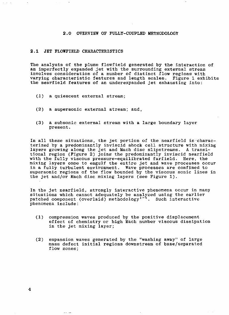
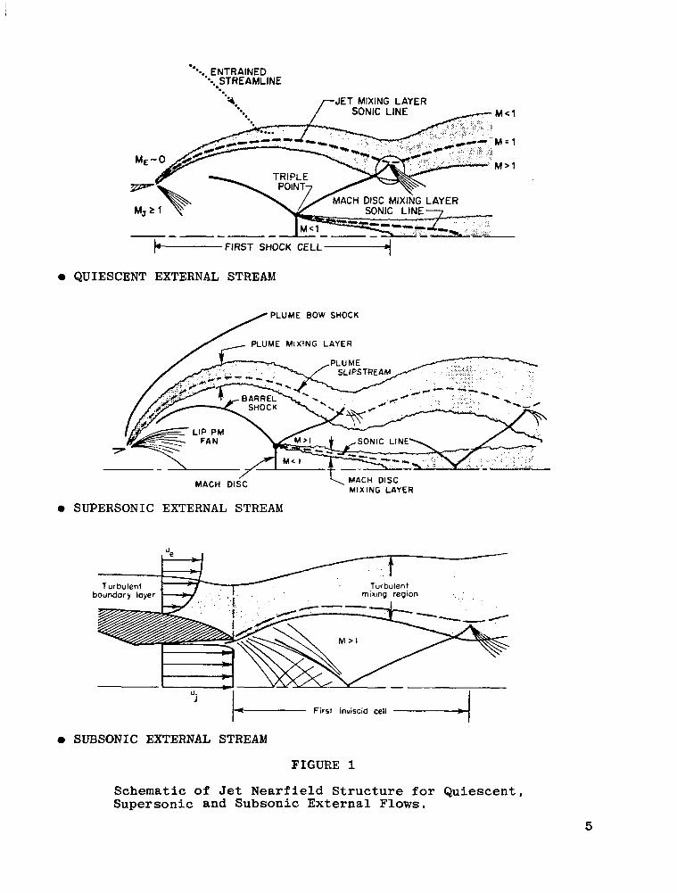

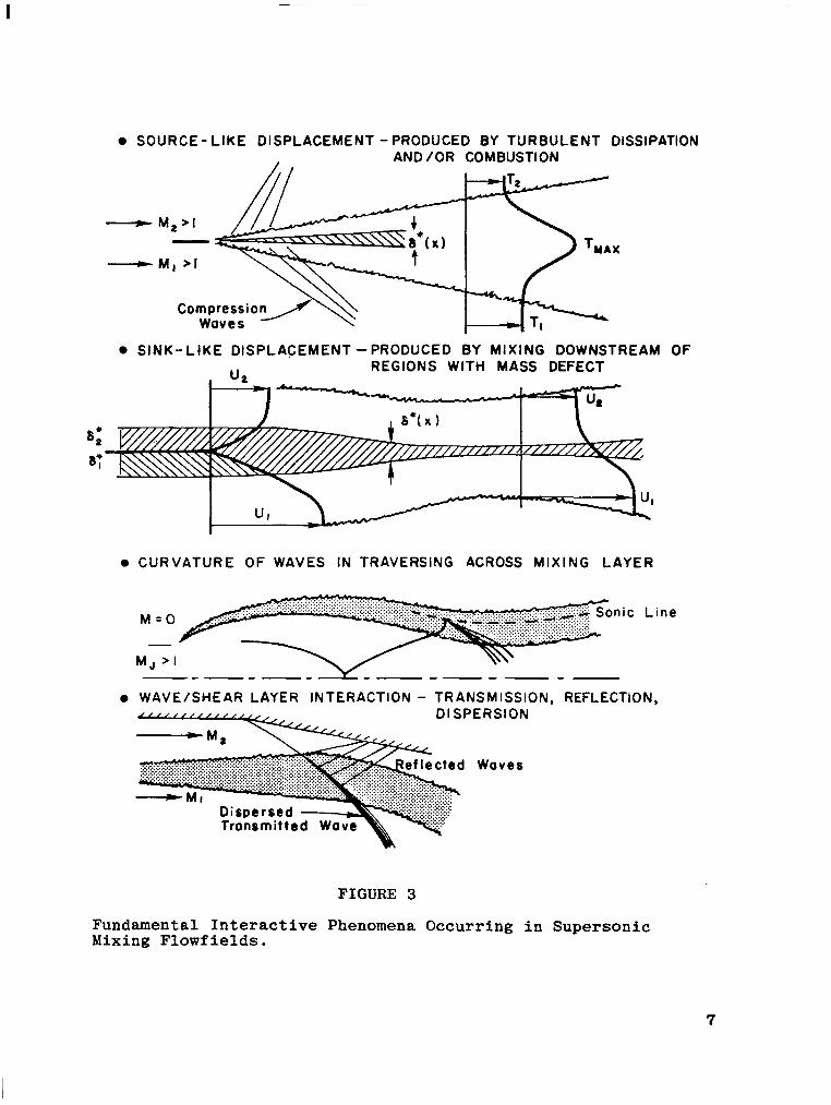


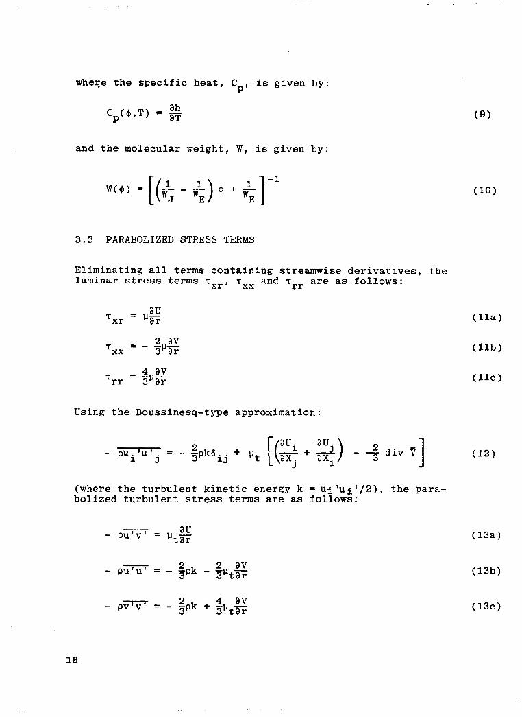


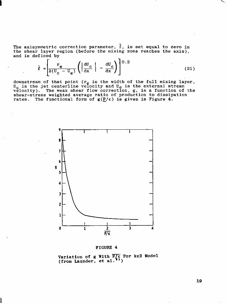


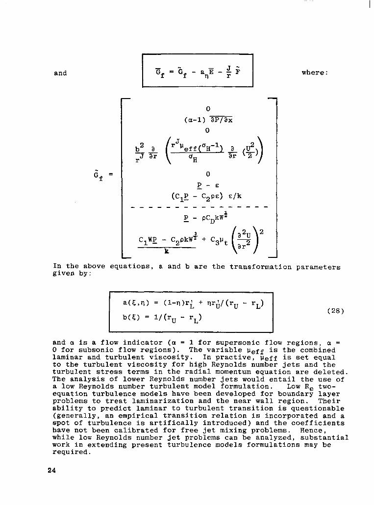

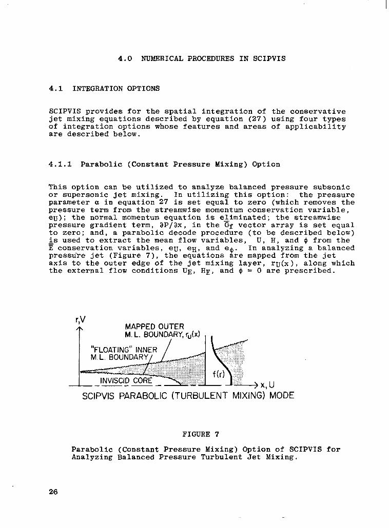

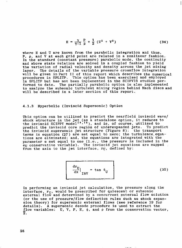


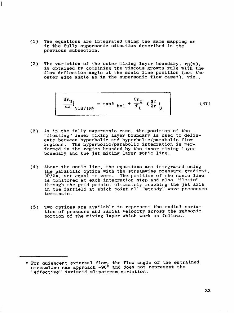
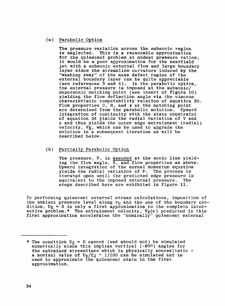
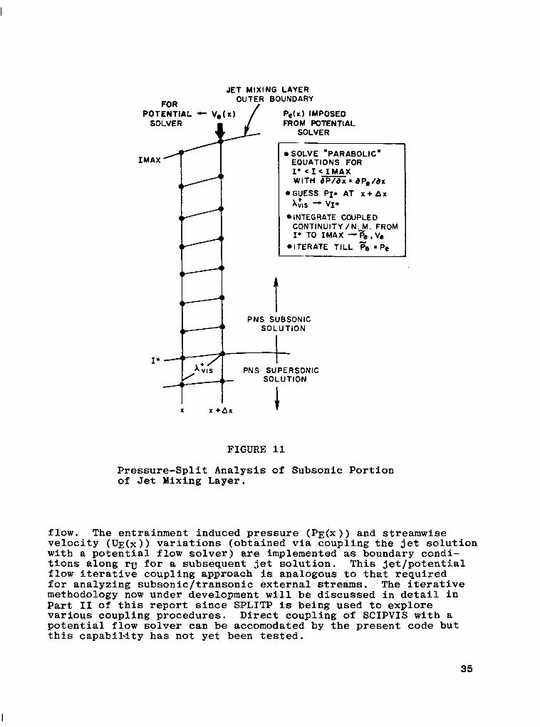
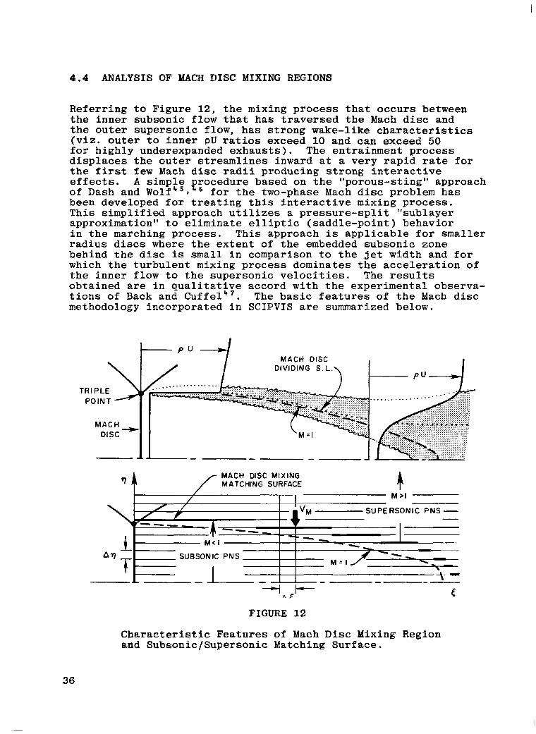
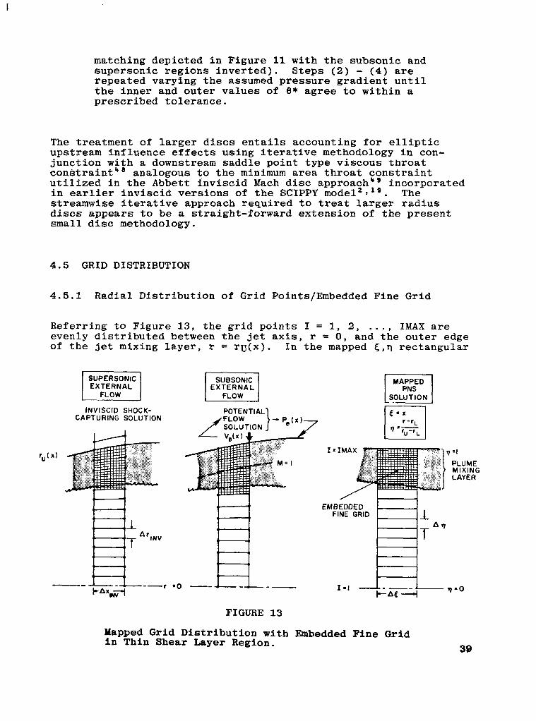


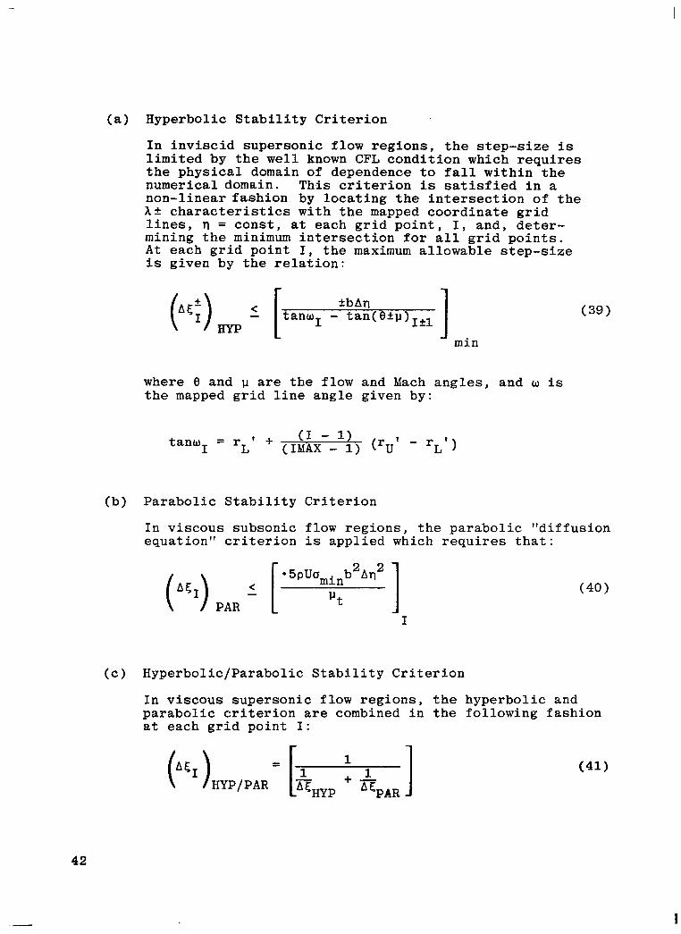


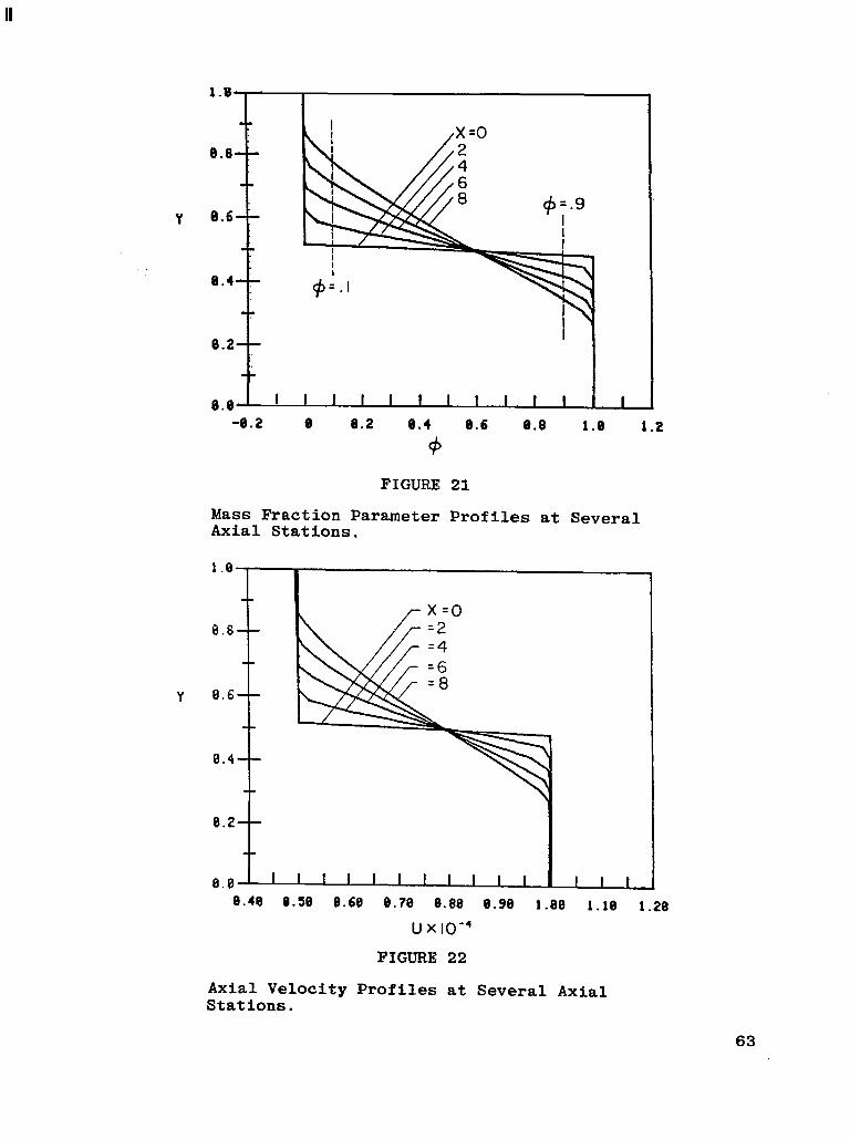

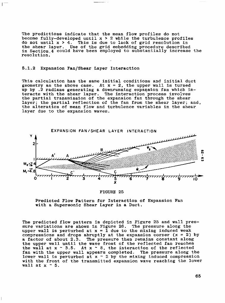

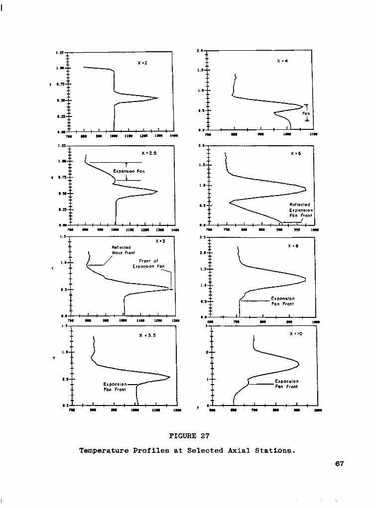


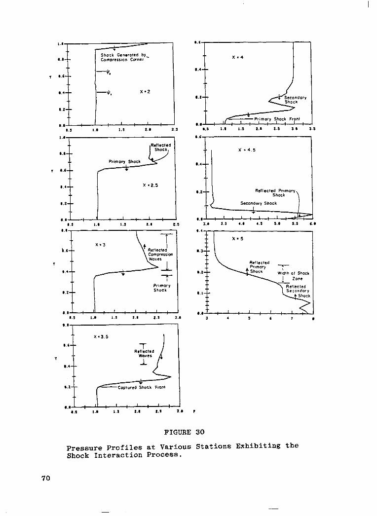
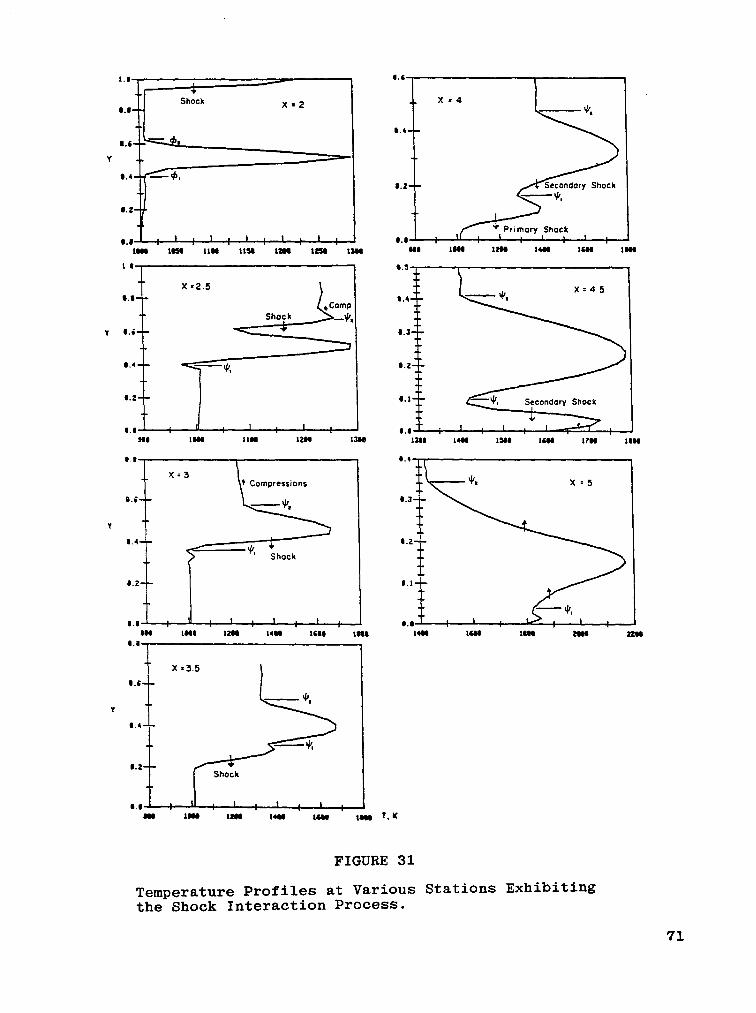

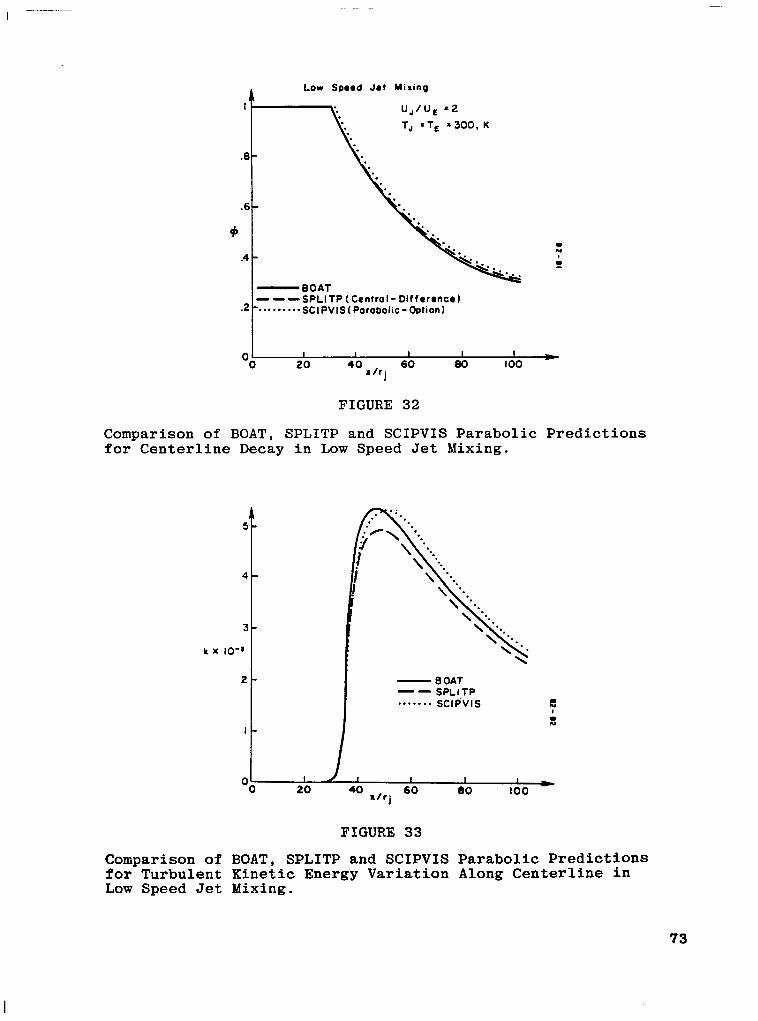
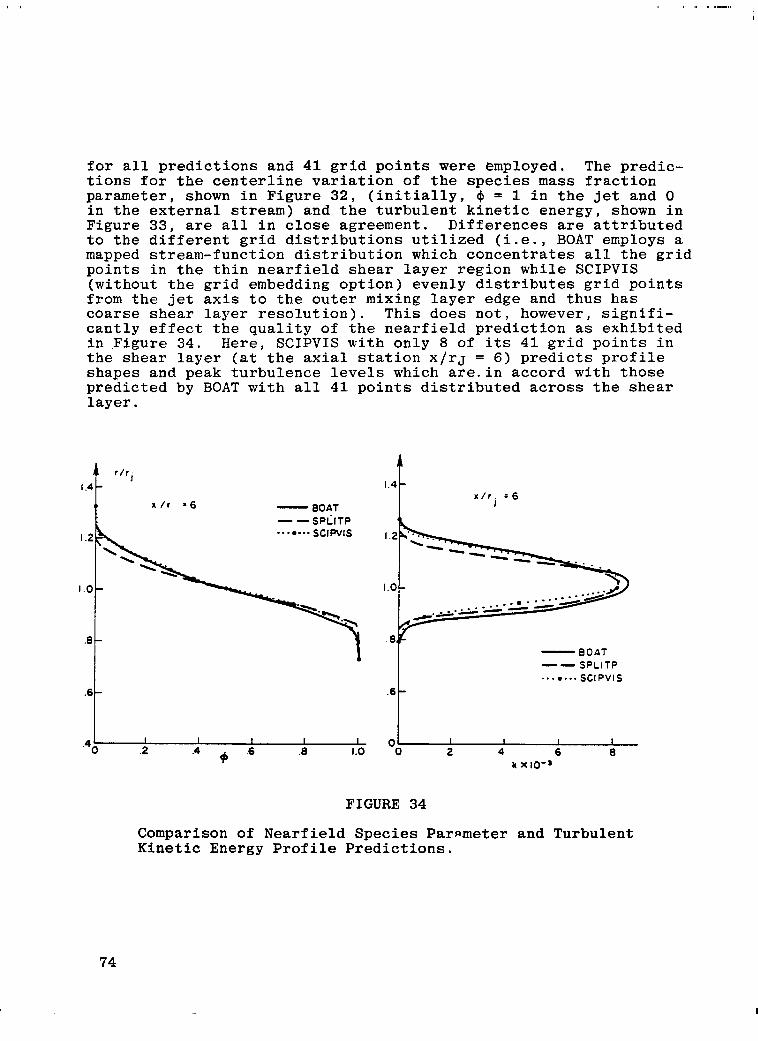

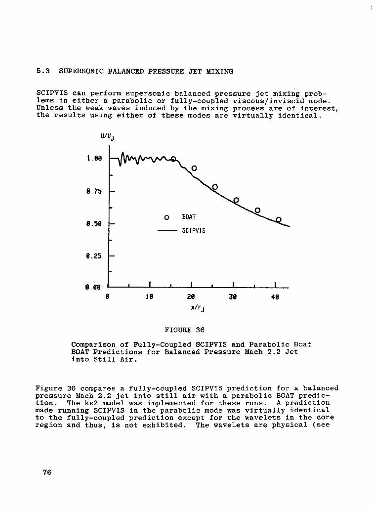
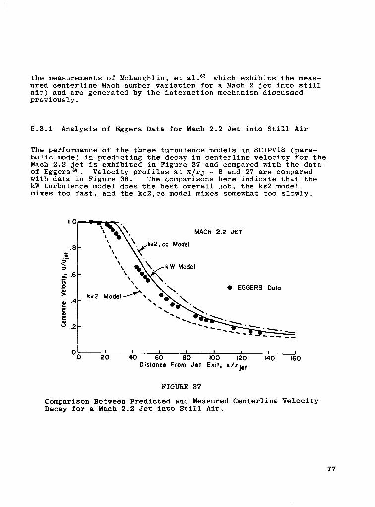


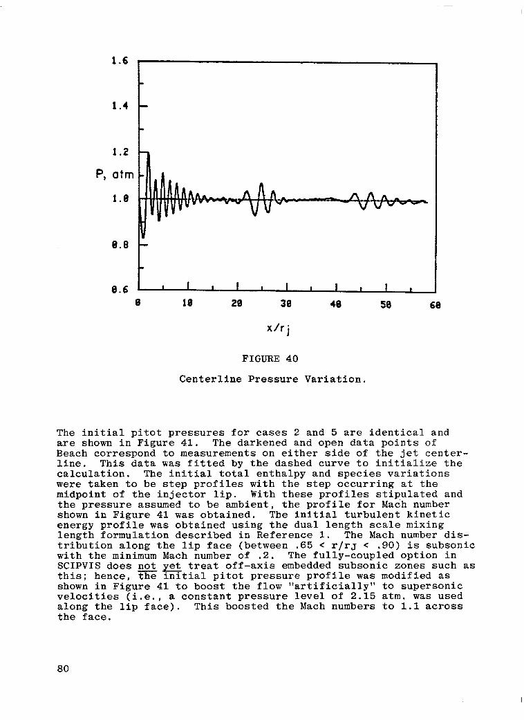


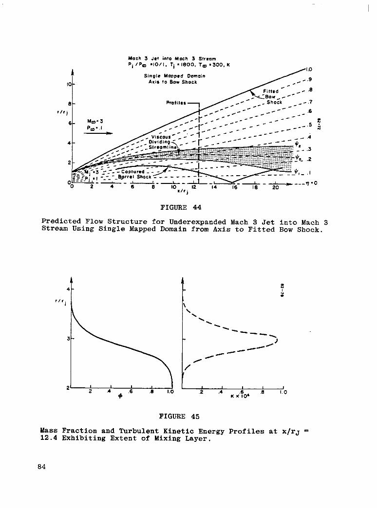


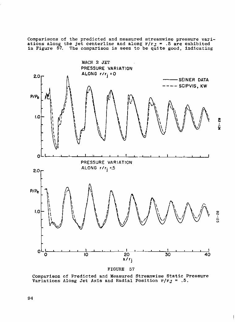
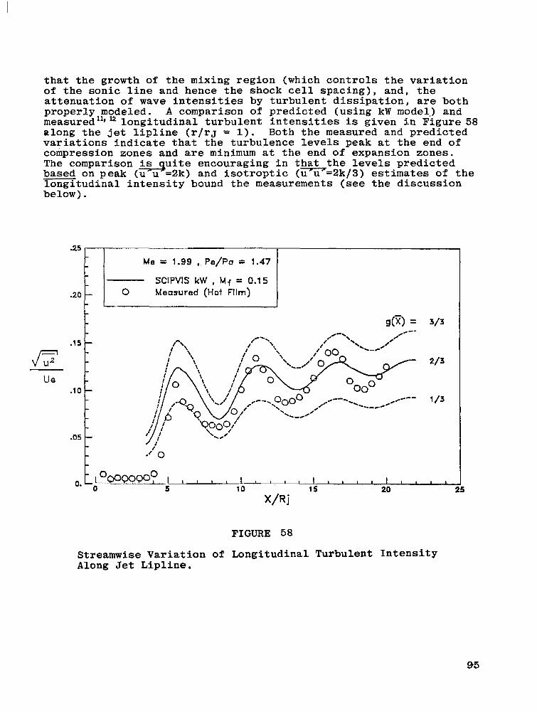
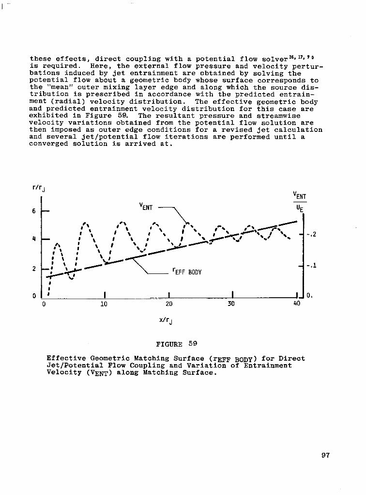


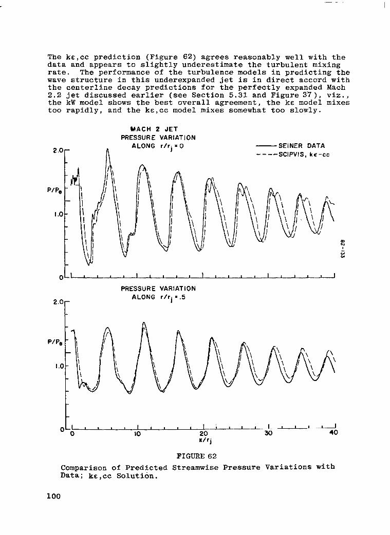


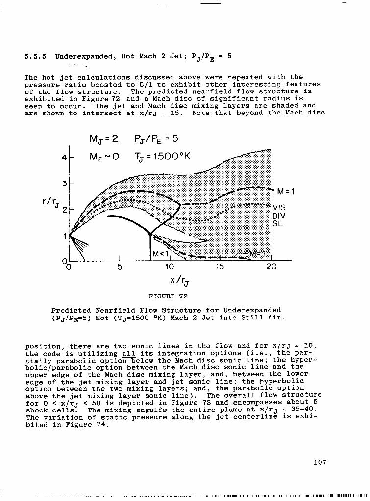


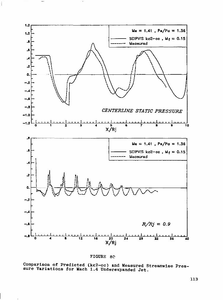


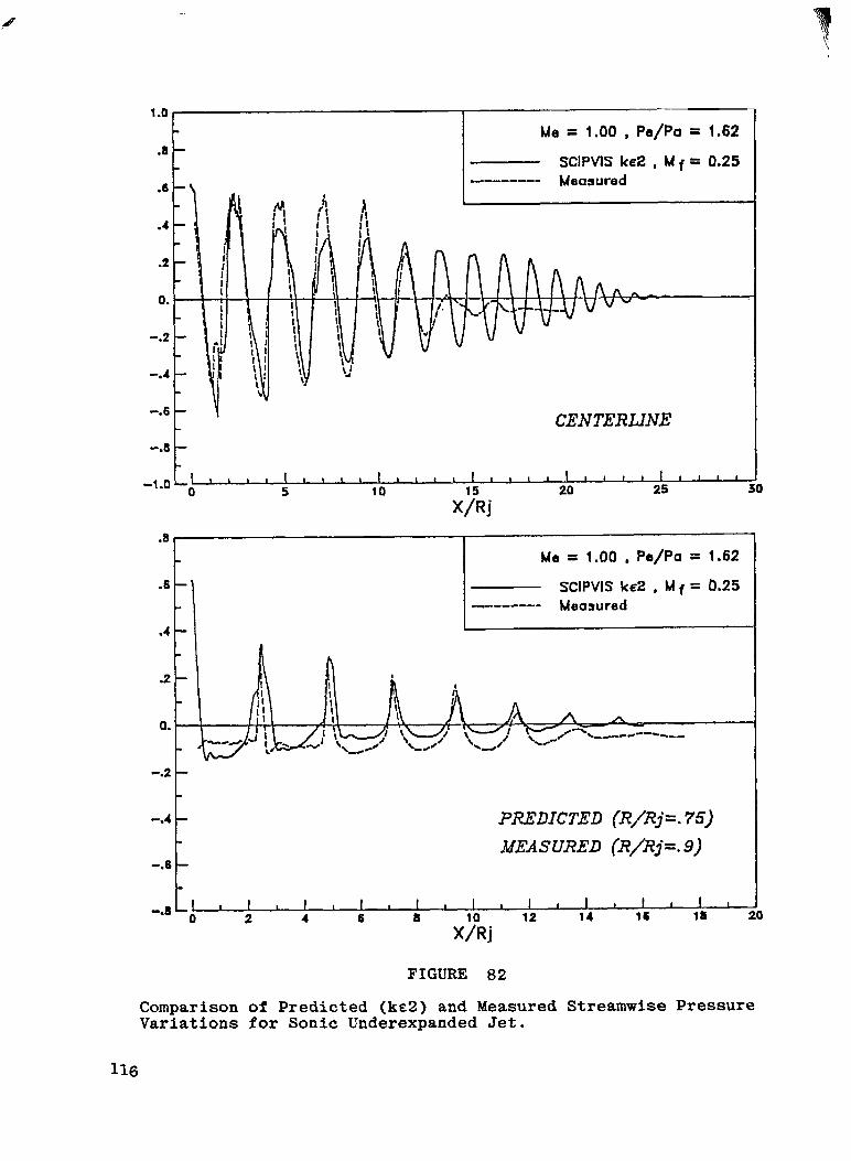


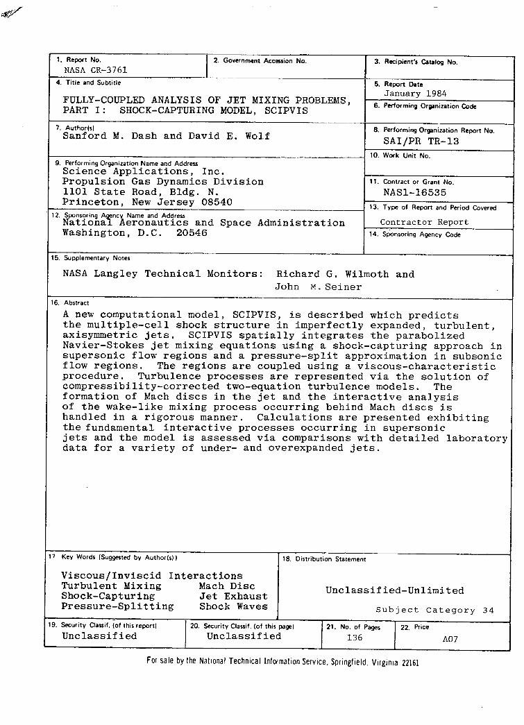


![5-2-3 Slurry Mixing w Pulse Jet Mixers_Perry Meyer[1]](https://static.documents.pub/doc/80x56/577d2ee01a28ab4e1eb03ae5/5-2-3-slurry-mixing-w-pulse-jet-mixersperry-meyer1.jpg)
