j ourna l homepage: www.e lsev ie r .com/ locate /mechmt
Function generation with the RRRCR spatial linkage
J. Jesús Cervantes-Sánchez ⁎, José M. Rico-Martínez, Víctor H. Pérez-Muñoz, Augustin BitangilagyUniversidad de Guanajuato, DICIS, Departamento de Ingeniería Mecánica, 36885, Palo Blanco, Salamanca, Guanajuato, Mexico
(A. Bitangilagy).1 For example, spatial mechanisms may be used in2 Symbols R, P, C and S stand for designating revolu3 In this paper, themost general architecture of a give
or 360°. See [12] for a detailed definition of the geom
A frequent requirement for the machine designer is that of generating an irregular motion. To this end, linkagesmay be used inindustrial applications to generate nonuniform motions which are not possible by gear trains otherwise [1].1 Under suchcircumstances, the output link has to rotate according to a function of the input motion.
Generation of a desired function (DF) may be achieved by using the input–output curve (IOC) of a linkage. Clearly, a perfectmatch between both functions seems to be an impossible task. However, experience indicates that we may achieve a perfectcoincidence of both functions only in certain points, which are usually known as precision points.
The process of forcing the IOC to match the DF in a certain number of precision points is what is known as exact kinematicsynthesis for function generation. This is a challenging and exciting discipline where the designer requires creativity andimagination as well as knowledge (mainly computational skills) and systematic thinking. As a rule of thumb, a larger number ofprecision points will imply a bigger effort in order to perform a successful synthesis process.
The synthesis for function generation is a motivating academic activity which has attracted the attention of several scholarsduring several decades. During this journey, several linkages ranging from planar, spherical and spatial have been proposed, seeTable 1 for a nonexhaustive sample of function generators.
In the search of new function generators, the RRRCR spatial linkage was found. There are very few studies concerning theRRRCR2 linkage. Almost three decades ago, Sticher [10,11] briefly described a method to obtain a maximum of 16 solutions for theclosures (number of ways in which a mechanism can be closed) of an RRRCR spatial linkage with the most general architecture.3
place of crossed helical gears and hypoid gears on skewed shafts [1].te, prismatic, cylindrical and spherical joints, respectively.n linkage means that each link has a length different from zero and a twist angle different from 0°, 90°, 180°etry associated with an arbitrary link.
Planar 4R 3 1955 Freudenstein [2]Planar 3RP 3 1964 Hartenberg and Denavit [3]Planar PRRP 3 1978 Suh and Radcliffe [4]Spherical 4R 4 1967 Zimmerman [5]Spherical 4R 5 2005 Alizade and Kilit [6]Spherical 4R 6 2009 Cervantes-Sánchez et al. [7]Spatial RSSP 6 1973 Rao et al. [8]Spatial RPSPR 6 2011 Cervantes-Sánchez et al. [9]
59J.J. Cervantes-Sánchez et al. / Mechanism and Machine Theory 74 (2014) 58–81
On the other hand, Alizade et al. [13] carried out the type synthesis of the RRRCR linkage as a byproduct of a method for typesynthesis of spatial mechanisms, which was based on the use of single-loop structural groups. Moreover, Fang and Tsai [14]reported a particular architecture of the RRRCR spatial linkage, which was conceived by means of a type synthesis procedurebased on the theory of reciprocal screws.
From the foregoing information, it may be concluded that only type synthesis and number synthesis have been addressed for theRRRCR spatial linkage. In addition to the type synthesis and number synthesis, and to the best knowledge of the authors, only akinematic position analysis of the RRRCR mechanism [15] has been reported. Hence the motivation to write this paper.
2. The RRRCR spatial linkage
It is important to distinguish between two different kinematic architectures associated with the spatial RRRCR linkage: thegeneral architecture and the particular architecture.
On the one hand, the most general architecture of the spatial RRRCR linkage is illustrated in Fig. 1. It should be noted thatoffsets are non-zero and skew angles between adjacent joint axes are not right angles. The mobility of this kinematic architectureis zero, i.e., the linkage is really an immovable structure [15]. However, by changing the relative orientation between motion axes,it is possible to obtain a spatial RRRCR linkage with one degree of freedom [15]. This particular architecture is shown in Fig. 2.
Referring to Fig. 2, it should be noted that the motion axes associated with the RC serial chain are parallel. However, themotion axes of the RRR planar chain are not parallel with the motion axes of the RC chain.
2.1. The input–output equation
In order to perform a systematic approach, it will be considered an arbitrary configuration of the particular RRRCR linkage, seeFigs. 3 and 4.
Fig. 1. Layout of the most general architecture of the RRRCR spatial linkage.
Fig. 2. Layout of the particular architecture of the RRRCR spatial linkage.
60 J.J. Cervantes-Sánchez et al. / Mechanism and Machine Theory 74 (2014) 58–81
After algebraic manipulation of the input–output equation (IOE) reported in [15], the following result is obtained:
Fig. 3. Geometry associated with the particular RRRCR spatial linkage: a general layout.
Fig. 4. Geometry associated with the particular RRRCR spatial linkage: details.
61J.J. Cervantes-Sánchez et al. / Mechanism and Machine Theory 74 (2014) 58–81
s1 = sin α1, c1 = cos α1, s2 ≡ sin α2 and c2 ≡ sin α2. Moreover, L, l, α1, α2, e, a, m, b and R are known as design parameters,
wherewhich characterize the kinematic architecture of the RRRCR linkage, such as it is shown in Figs. 3 and 4. It is important to realizethat Eq. (1) does not depend on the design parameter m.
Eq. (1) is the input–output equation associated with the particular architecture of the RRRCR spatial linkage.Moreover, for the purposes of this paper, angles θ and ϕ will be considered as the input and output variables,respectively. In this way, angle θ represents the rotation of input link 1, whereas angle ϕ characterizes the rotation ofthe output link 4.
3. Kinematic synthesis
This section deals with the problem of designing a spatial RRRCR linkage such that to six given orientations of the inputlink, defined by angles {θ}16, correspond six prescribed orientations of the output link, {θ}16. Such a set of six pairs of values,namely (θi,ϕi), will be extracted from what is known as desired function, i.e., the function to be satisfied. Thus, the mainpurpose of this section is to find a linkage which exactly satisfies the desired function at the precision points, which arerepresented by (θi,ϕi).
After several attempts, it was concluded that the best synthesis approach is to find the values of only six design parameters,namely, L, l, α1, α2, a and R, for six precision points (θ1,ϕ1), (θ2,ϕ2), ts, (θ6,ϕ6). The remaining design parameters, namely,m, b ande, are left to the convenience of the designer. To this end, as it will be shown later, the proposed approach will be mainly based onthe input–output Eq. (1).
62 J.J. Cervantes-Sánchez et al. / Mechanism and Machine Theory 74 (2014) 58–81
3.1. Design equations
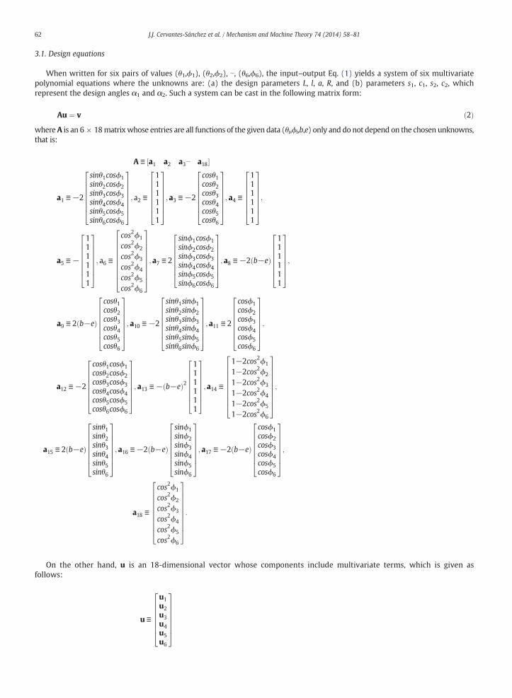
When written for six pairs of values (θ1,ϕ1), (θ2,ϕ2), ⋯, (θ6,ϕ6), the input–output Eq. (1) yields a system of six multivariatepolynomial equations where the unknowns are: (a) the design parameters L, l, a, R, and (b) parameters s1, c1, s2, c2, whichrepresent the design angles α1 and α2. Such a system can be cast in the following matrix form:
a15
Au ¼ v ð2ÞA is an 6 × 18matrixwhose entries are all functions of the given data (θi,ϕi,b,e) only and do not depend on the chosen unknowns,
On the other hand, u is an 18-dimensional vector whose components include multivariate terms, which is given asfollows:
u≡
u1u2u3u4u5u6
26666664
37777775
where
Fig. 5. Plot of the desired function, y = x0.6.
63J.J. Cervantes-Sánchez et al. / Mechanism and Machine Theory 74 (2014) 58–81
:
u1 ≡s1c1s2c2LRc21c
22a
2
c21c22aL
24
35;u2 ≡
c21c22L
2
c21c22l
2
c21c22R
2
264
375;u3 ≡
s1c1s2R2
s1c1c22a
s1c1c22L
264
375;
u4 ≡c21c2LRc1c
22aR
c1c22LR
264
375;u5 ≡
c21c22
c21R2
c1s2c2L
264
375;u6 ≡
c1s2Rs1RR2
24
35:
Finally, v is an 6-dimensional vector given by:
v ≡− b−eð Þ2
111111
26666664
37777775:
Additionally, it should be noted that, due to the trigonometric nature of unknowns s1, c1, s2 and c2, they are subjected to thefollowing quadratic constraints:
s21 þ c21 ¼ 1; s22 þ c22 ¼ 1: ð3Þ
Summarizing, Eqs. (2) and (3) constitute a system of 8 multivariate polynomial equations in 8 unknowns, which are calleddesign equations.
3.2. Solution of the design equations
Design Eqs. (2) and (3) need to be solved for the eight unknowns L, l, a, R, s1, c1, s2 and c2. However, and because of the highlynonlinear and extremely complex nature of the design equations, multiple solutions are expected. Such a set of solutions willcorrespond to different possible design parameters of the linkage under study.
Fig. 6. The RRRCR spatial linkage at the first precision point: θ1 = 47.45°, ϕ1 = 48.13° and generated function y = x0.6.
64 J.J. Cervantes-Sánchez et al. / Mechanism and Machine Theory 74 (2014) 58–81
3.3. Computation of design parameters
On the one hand, it is important to remember that, from the whole set of design parameters, namely, L, l, α1, α2, e, a,m, b and R,only numerical values of m, b and e will be left to the designer's disposal.
On the other hand, it is expected that the computer package provides one real solution at least. Thus, numerical values for L, l,a, R, s1, c1, s2 and c2 will be available at this point. Then, all remaining is to convert the numerical values of s1, c1, s2 and c2 into thecorresponding values of design angles α1 and α2. To this end, and since the sine and cosine of the design angles are alreadyknown, then the unique and correct value of the corresponding angle defined by them can be readily computed as follows[21]:
where
α1 ¼ 2arctans1
1þ c1
� �; c1≠−1 ð4Þ
α2 ¼ 2arctans2
1þ c2
� �; c2≠−1 ð5Þ
, if c1 = −1 or c2 = −1, these equations cannot be used, but in that case, α1 = 180° or α2 = 180°, respectively.
4. Application examples
Three challenging examples are used in order to show the applicability of the approach proposed here. These examples involveintricate planar curves to be generated by the RRRCR spatial linkage.
Fig. 7. The RRRCR spatial linkage at the second precision point: θ2 = 66.08°, ϕ2 = 70.71° and generated function y = x0.6.
65J.J. Cervantes-Sánchez et al. / Mechanism and Machine Theory 74 (2014) 58–81
4.1. Algebraic function
This first example considers an algebraic function given by:
y ¼ x0:6 ð6Þdesired function to be generated by the RRRCR spatial linkage.
as the
Additionally, the interval of interest for this first example is required to be 1 ≤ x ≤ 3.Next, in order to follow a systematic approach, we establish now that angular displacement θ of the input link will be
proportional to independent variable x and angular displacement ϕ of the output link will be proportional to dependentvariable y.
Thus, once the desired function and the interval of interest have been chosen, the next task is to use Chebyshev spacing overthe range to minimize structural error [22]. Then, the corresponding values of the variables x and y are:
Fig. 8. The RRRCR spatial linkage at the third precision point: θ3 = 98.36°, ϕ3 = 105.91° and generated function y = x0.6.
66 J.J. Cervantes-Sánchez et al. / Mechanism and Machine Theory 74 (2014) 58–81
For the particular case under study, a graphical illustration of Chebyshev spacing is shown in Fig. 5.Next, the initial values for angles θ and ϕ are chosen as follows:
θ0 ¼ 45�
ϕ0 ¼ 45�:
We are also free to select the ranges of variation of angles θ and ϕ:
Δθ ¼ 144� ¼ 4π5
� �rad
Δϕ ¼ 144� ¼ 4π5
� �rad:
Going further, the resulting precision points are given by:
θ1 ¼ 0:828217032920411 rad 47:45�� �; ϕ1 ¼ 0:840090531599455 rad 48:13�� �
θ2 ¼ 1:153458637201692 rad 66:08�� �; ϕ2 ¼ 1:234203348399758 rad 70:71�� �
θ3 ¼ 1:716793620552084 rad 98:36�� �; ϕ3 ¼ 1:848637086284091 rad 105:91�� �
θ4 ¼ 2:367276829114647 rad 135:63�� �; ϕ4 ¼ 2:483561355233873 rad 142:29�� �
θ5 ¼ 2:930611812465039 rad 167:91�� �; ϕ5 ¼ 2:987438659689003 rad 171:16�� �
θ6 ¼ 3:255853416746321 rad 186:54�� �; ϕ6 ¼ 3:263109789045178 rad 186:96�� �
:
(a) Front view
135.63o
142.30o
(b) 3D view
Fig. 9. The RRRCR spatial linkage at the fourth precision point: θ4 = 135.63°, ϕ4 = 142.29° and generated function y = x0.6.
67J.J. Cervantes-Sánchez et al. / Mechanism and Machine Theory 74 (2014) 58–81
With these results, and recalling Eqs. (4) and (5), the remaining design parameters are found as:
α1 ¼ 39:0363929433�;α2 ¼ −14:5153256147�
:
notation u.l. stands for tect arbitrary units of length.selection criteria were: (a) non-zero and positive link lengths, and (b) a maximum relation between link lengths equal to four.
(a) Front view
(b) 3D view
Fig. 10. The RRRCR spatial linkage at the fifth precision point: θ5 = 167.91°, ϕ5 = 171.16° and generated function y = x0.6.
68 J.J. Cervantes-Sánchez et al. / Mechanism and Machine Theory 74 (2014) 58–81
Before finishing, the residuals in the design equations were analyzed. The magnitude of the residuals was always better than2.79 × 10−9, thus showing a high level of numerical accuracy.
Additionally, a computer package for solid modeling was used in order to illustrate the RRRCR spatial linkage at the sixdifferent configurations associated with the precision points. They are shown in Figs. 6–11.
A careful observation of the resulting linkage reveals that the lengths of the different links are very similar compared eachother. Hence, the synthesized linkage has a good index of proportionality between link lengths, which is difficult to be achievedwhen designing a linkage.
Additionally, in order to complete the evaluation of the synthesized linkage, Figs. 12–13 show the function generated by thelinkage, and a superposition of the desired function and the function generated by the linkage, respectively.
As it can be seen in Fig. 13, the desired function and the function generated by the RRRCR spatial linkage coincide perfectly atthe precision points.
4.2. Archimedean spiral
The desired function for this second example is given by:
which
x tð Þ ¼ 2−5tsin tð Þ;
y tð Þ ¼ 2þ 5tcos tð Þ:
ð7Þ
is known as Archimedean spiral.
(a) Front view
(b) 3D view
Fig. 11. The RRRCR spatial linkage at the sixth precision point: θ6 = 186.55°, ϕ6 = 186.96° and generated function y = x0.6.
69J.J. Cervantes-Sánchez et al. / Mechanism and Machine Theory 74 (2014) 58–81
Due to the parametric nature of the desired function, we may choose the initial and final values of parameter t. To this end, sixprecision points are taken in the range − 8 ≤ t ≤ −5 with Chebyshev spacing, thus yielding:
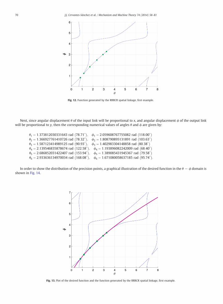
Fig. 12. Function generated by the RRRCR spatial linkage, first example.
70 J.J. Cervantes-Sánchez et al. / Mechanism and Machine Theory 74 (2014) 58–81
Next, since angular displacement θ of the input link will be proportional to x, and angular displacement ϕ of the output linkwill be proportional to y, then the corresponding numerical values of angles θ and ϕ are given by:
θ1 ¼ 1:373812030331643 rad 78:71�� �; ϕ1 ¼ 2:059608767755082 rad 118:00�� �
θ2 ¼ 1:366927761410726 rad 78:32�� �; ϕ2 ¼ 1:808790895131891 rad 103:63�� �
θ3 ¼ 1:587123414989125 rad 90:93�� �; ϕ3 ¼ 1:402983304148858 rad 80:38�� �
θ4 ¼ 2:139546835878674 rad 122:58�� �; ϕ4 ¼ 1:193896082242009 rad 68:40�� �
θ5 ¼ 2:686852031422407 rad 153:94�� �; ϕ5 ¼ 1:389085431945367 rad 79:58�� �
θ6 ¼ 2:933636134970034 rad 168:08�� �; ϕ6 ¼ 1:671080058637185 rad 95:74�� �
:
In order to show the distribution of the precision points, a graphical illustration of the desired function in the θ − ϕ domain isshown in Fig. 14.
Fig. 13. Plot of the desired function and the function generated by the RRRCR spatial linkage, first example.
Fig. 14. Plot of the Archimedean spiral.
71J.J. Cervantes-Sánchez et al. / Mechanism and Machine Theory 74 (2014) 58–81
Fig. 15. The RRRCR spatial linkage at the first precision point: θ1 = 78.71°, ϕ1 = 118.00°, Archimedean spiral.
Fig. 16. The RRRCR spatial linkage at the second precision point: θ2 = 78.32°, ϕ2 = 103.63°, Archimedean spiral.
Fig. 17. The RRRCR spatial linkage at the third precision point: θ3 = 90.93°, ϕ3 = 80.38°, Archimedean spiral.
72 J.J. Cervantes-Sánchez et al. / Mechanism and Machine Theory 74 (2014) 58–81
Fig. 18. The RRRCR spatial linkage at the fourth precision point: θ4 = 122.58°, ϕ4 = 68.40°, Archimedean spiral.
Fig. 19. The RRRCR spatial linkage at the fifth precision point: θ5 = 153.94°, ϕ5 = 79.58°, Archimedean spiral.
73J.J. Cervantes-Sánchez et al. / Mechanism and Machine Theory 74 (2014) 58–81
Fig. 20. The RRRCR spatial linkage at the sixth precision point: θ6 = 168.08°, ϕ6 = 95.74°, Archimedean spiral.
74 J.J. Cervantes-Sánchez et al. / Mechanism and Machine Theory 74 (2014) 58–81
operating system, and after a computational time of around 19.2 h, 1616 solutions were obtained. From these solutions, only 120solutions were real. Based on the selection criteria presented in the first example, the following solution was found:
After design parameters were computed, the residuals in the design equations were verified. The magnitude of the residualswas always better than 6.8 × 10⁻¹⁰, thus showing an excellent numerical accuracy.
Finally, by using a computer package for solid modeling, the RRRCR spatial linkage was drawn at the six differentconfigurations associated with the precision points. The resulting solid models are shown in Figs. 15–20.
Fig. 23. Plot of the desired function, third example.
Fig. 24. The RRRCR spatial linkage at the first precision point: θ1 = 41.70°, ϕ1 = 58.44°, trigonometric function.
Fig. 25. The RRRCR spatial linkage at the second precision point: θ2 = 54.64°, ϕ2 = 65.61°, trigonometric function.
76 J.J. Cervantes-Sánchez et al. / Mechanism and Machine Theory 74 (2014) 58–81
Fig. 26. The RRRCR spatial linkage at the third precision point: θ3 = 77.06°, ϕ3 = 93.57°, trigonometric function.
77J.J. Cervantes-Sánchez et al. / Mechanism and Machine Theory 74 (2014) 58–81
Additionally, in order to complete the evaluation of the resulting linkage, Fig. 21 shows the function generated by thesynthesized linkage. Moreover, Fig. 22 shows a superposition of the desired function and the function generated by the linkage.
Before concluding this example, it should be noted that the desired function and the function generated by the RRRCR spatiallinkage coincide perfectly at the precision points, see Fig. 22.
4.3. Trigonometric function
An intricate trigonometric function was selected for this third example:
y ¼ cos 2x−π=2ð Þ3 þ 2sin x=2ð Þ ð8Þ
is highly nonlinear.
whichUsing Chebyshev spacing over the range π/4 ≤ x ≤ 3π/4, then the corresponding values for the Cartesian coordinates x and y
In order to show the resulting spacing, a graphical illustration is shown in Fig. 23.
Fig. 27. The RRRCR spatial linkage at the fourth precision point: θ4 = 102.94°, ϕ4 = 81.11°, trigonometric function.
78 J.J. Cervantes-Sánchez et al. / Mechanism and Machine Theory 74 (2014) 58–81
Since we can choose arbitrarily the initial values for angles θ and ϕ, then:
θ0 ¼ 40� ¼ 2π9
� �rad
ϕ0 ¼ 60� ¼ π3
� �rad:
We are also free to select the angular ranges of the input and output motions, namely Δθ = 100° and Δϕ = 70°. Thus, theprecision points are given by:
θ1 ¼ 0:727867026855344 rad 41:70�� �; ϕ1 ¼ 1:020082406910900 rad 58:44�� �
θ2 ¼ 0:953729252050679 rad 54:64�� �; ϕ2 ¼ 1:145229947554650 rad 65:61�� �
θ3 ¼ 1:344934101599562 rad 77:06�� �; ϕ3 ¼ 1:633164973182138 rad 93:57�� �
θ4 ¼ 1:796658551990231 rad 102:94�� �; ϕ4 ¼ 1:415736576153583 rad 81:11�� �
θ5 ¼ 2:187863401539114 rad 125:35�� �; ϕ5 ¼ 2:028492127576434 rad 116:22�� �
θ6 ¼ 2:413725626734449 rad 138:29�� �; ϕ6 ¼ 2:277071611636885 rad 130:46�� �
:
Once the precision points are known, the next task is to give numerical values to the free design parametersm, b, and e. Thesevalues are arbitrarily chosen as m = 1.5 u.l., b = 2.0 u.l., and e = 1.5 u.l.
With these results, and recalling Eqs. (4) and (5), the remaining design parameters resulted as follows:
α1 ¼ 177:5834861970�;α2 ¼ −113:5865852664�
:
After design parameters are known, the residuals in the design equations were verified. The magnitude of the residuals wasalways better than 3.6 × 10⁻⁹, showing a high level of numerical accuracy.
At this point, the synthesis of the RRRCR spatial linkage is complete. However, a convenient way to visualize the resultingnumerical values is through solid models of the synthesized linkage. To this end, the resulting design parameters were used as theinput in a computer package for solid modeling. Thus, the computer provides virtual models of the RRRCR spatial linkage on agraphic display screen. The resulting drawings for the six different configurations associated with the precision points are shownin Figs. 24–29.
A careful observation of the resulting linkage reveals that the lengths of the different links are very similar compared eachother. Hence, the synthesized linkage has a good index of proportionality between link lengths, which is difficult to be achievedwhen designing a linkage.
Before finishing, it is important to realize that the quality of the design may be evaluated by means of the inspection of thedesired function and the function generated by the synthesized linkage. In this regard, Fig. 30 shows the function generated by thelinkage, and Fig. 31 shows a superposition of the desired function and the function generated by the linkage.
As it can be seen in Fig. 31, the desired function and the function generated by the RRRCR spatial linkage show a good match atthe precision points.
Fig. 28. The RRRCR spatial linkage at the fifth precision point: θ5 = 125.35°, ϕ5 = 116.22°, trigonometric function.
Fig. 29. The RRRCR spatial linkage at the sixth precision point: θ6 = 138.29°, ϕ6 = 116.46°, trigonometric function.
80 J.J. Cervantes-Sánchez et al. / Mechanism and Machine Theory 74 (2014) 58–81
5. Conclusions
It has been presented a synthesis approach for the function generation of the RRRCR spatial linkage with six precision points. Acareful observation of the resulting linkages reveals that the lengths of the different links are very similar compared each other.Hence, the synthesized linkages have a good index of proportionality between link lengths, which is a difficult task whendesigning a linkage. Moreover, the magnitude of the residuals in the design equations was always better than 3.611 × 10⁻⁹,which indicates a very good level of numerical accuracy. Finally, in two of the three cases, there is a good agreement between thedesired and generated functions in the interval defined by the precision points. It remains to investigate the possible presence of
Fig. 30. Function generated by the RRRCR spatial linkage, third example.
Fig. 31. Plot of the desired function and the function generated by the RRRCR spatial linkage, third example.
81J.J. Cervantes-Sánchez et al. / Mechanism and Machine Theory 74 (2014) 58–81
the order, branch and rotatability problems. In particular, the branching seems to be a very challenging problem due to the bi- andtetra-modal nature of the RRRCR linkage [15].
Acknowledgments
The authors acknowledge the support of the Consejo Nacional de Ciencia y Tecnología (National Council of Science andTechnology, CONACYT), of México, through SNI (National Network of Researchers) fellowships and scholarships.
References
[1] C. Bagci, Geometric methods for the synthesis of spherical mechanisms for the generation of functions, paths and rigid-body positions using conformalprojections, Mech. Mach. Theory 19 (1) (1984) 113–127.
[2] F. Freudenstein, Approximate synthesis of four-bar linkages, Trans. ASME 77 (1955) 853–861.[3] R.S. Hartenberg, J. Denavit, Kinematic Synthesis of Linkages, McGraw-Hill, 1964. 308–311.[4] C.H. Suh, C.W. Radcliffe, Kinematics and Mechanism Design, John Wiley & Sons, 1978. 172–173.[5] J.R. Zimmerman, Four-precision-point synthesis of the spherical four-bar function generator, J. Mech. 2 (1) (1967) 133–139.[6] R.I. Alizade, O. Kilit, Analytic synthesis of function generating spherical four-bar mechanism for the five precision points, Mech. Mach. Theory 40 (7) (2005)
863–878.[7] J.J. Cervantes-Sánchez, L. Gracia, J.M. Rico-Martínez, H.I. Medellín-Castillo, J.E. González-Galván, A novel and efficient kinematic synthesis approach of the
spherical 4R function generator for five and six precision points, Mech. Mach. Theory 44 (11) (2009) 2020–2037.[8] A.V.M. Rao, G.N. Sandor, D. Kohli, A.H. Soni, Closed form synthesis of spatial function generating mechanisms for the maximum number of precision points,
Trans. ASME J. Eng. Ind. 725–736 (August 1973).[9] J.J. Cervantes-Sánchez, L. Gracia, E. Alba-Ruiz, J.M. Rico-Martínez, Synthesis of a special RPSPR spatial linkage function generator for six precision points, Mech.
Mach. Theory 46 (1) (2011) 83–96.[10] F. Sticher, The concept of point-line systems in predicting the number of closures of some spatial linkages, Mech. Mach. Theory 16 (1981) 197–214.[11] F. Sticher, Closures of spatial mechanisms via line systems theory, 2nd IFToMM Symp. Linkages and Computer Aided Design Meth., Bucharest, Romania, Vol.
II, Paper No. 33, 1977.[12] C.D. Crane III, J. Duffy, Kinematic Analysis of Robot Manipulators, Cambridge University Press, New York, 1998. 20–21.[13] R.I. Alizade, G.N. Sandor, Determination of the condition of existence of complete crank rotation and of the instantaneous efficiency of spatial four-bar
mechanisms, Mech. Mach. Theory 20 (1985) 155–163.[14] Y. Fang, L.W. Tsai, Enumeration of a class of overconstrained mechanisms using the theory of reciprocal screws, Mech. Mach. Theory 39 (2004) 1175–1187.[15] J.J. Cervantes-Sánchez, J.M. Rico, L. Gracia, A. Tadeo-Chávez, G.I. Pérez-Soto, L.D. Aguilera, Kinematic position analysis of a notable bi-tetra-modal linkage: the
RRRCR spatial linkage, Proc. 13th World Congress in Mechanism and Machine Science, Guanajuato, Gto., México, June, 19–25, 2011, 2011.[16] J. Nielsen, B. Roth, Formulation and solution for the direct and inverse kinematics problems for mechanisms and mechatronic systems, in: J. Angeles, E.
Zakhariev (Eds.), Computational Methods in Mechanical Systems: Mechanism Aanalysis, Synthesis, and Optimization, NATO ASI Series, vol. 161, 1998,pp. 33–52.
[17] C.W. Wampler, A.P. Morgan, A.J. Sommese, Numerical continuation methods for solving polynomial systems arising in kinematics, Trans. ASME J. Mech. Des.112 (1) (1990) 59–68.
[18] D.J. Bates, J.D. Hauenstein, A.J. Sommese, C.W. Wampler, Software for numerical algebraic geometry: a paradigm and progress towards its implementation,IMA Math. Appl., vol. 148, Springer, New York, 2008. 1–14.
[19] E. Gross, S. Petrovic, J. Verschelde, Interfacing with PHCpack, J. Softw. Algebra Geom. 5 (2013) 20–25.[20] W. Rheinboldt, Methods for solving systems of nonlinear equations, Society for Industrial and Applied Mathematics, Second ed., 1998. 85.[21] K.C. Gupta, Mechanics and Control of Robots, Springer, 1997. 51.[22] K.J. Waldron, G.L. Kinzel, Kinematics, Dynamics, and Design of Machinery, John Wiley & Sons, 1999. 263–264.