1 Functional Analysis and Applications Lecture notes for MATH 797fn Luc Rey-Bellet University of Massachusetts Amherst The functional analysis, usually understood as the linear theory, can be described as Extension of linear algebra to infinite-dimensional vector spaces using topological concepts The theory arised gradually from many applications such as solving boundary value problems, solving partial differential equations such as the wave equation or the Schr¨ odinger equation of quantum mechanics, etc... Such problems lead to a comprehensive analysis of function spaces and their structure and of linear (an non-linear) maps acting on function spaces. These concepts were then reformulated in abstract form in the modern theory of functional analysis. Functional analytic tools are used in a wide range of applications, some of which we will discuss in this class.
Transcript
1
Functional Analysis and Applications
Lecture notes for MATH 797fn
Luc Rey-BelletUniversity of Massachusetts Amherst
The functional analysis, usually understood as the linear theory, can be described as
Extension of linear algebra to infinite-dimensionalvector spaces using topological concepts
The theory arised gradually from many applications such as solving boundary value problems, solvingpartial differential equations such as the wave equation or the Schrodinger equation of quantum mechanics,etc... Such problems lead to a comprehensive analysis of function spaces and their structure and of linear(an non-linear) maps acting on function spaces. These concepts were then reformulated in abstract form inthe modern theory of functional analysis. Functional analytic tools are used in a wide range of applications,some of which we will discuss in this class.
2
Chapter 1
Metric Spaces
1.1 Definitions and examplesOne can introduce a topology on some set M by specifying a metric on M .
Definition 1.1. A map d(·, ·) : M ×M → R is called a metric on the set M if for all ξ, η, ζ ∈M we have
1. (positive definite) d(ξ, η) ≥ 0 and d(ξ, η) = 0 if and if ξ = η.
1. M = C[a, b] with d(f, g) =∫ ba|f(t)− g(t)|p dt with 0 < p <∞.
2. M = C[a, b] with d(f, g) = maxt∈[a,b] |f(t)− g(t)|
3. For any measure space (X,µ), M = Lp(X,µ) with d(f, g) = ‖f − g‖p with 1 ≤ p ≤ ∞.
4. Let M be the set of all infinite sequences ξ = (x1, x2, · · · ) with xi ∈ C. Then for η = (y1, y2, · · · )
d(ξ, η) =
∞∑i=1
(1
2
)i |xi − yi|1 + |xi − yi|
(1.1)
defines a metric on M .
5. Let M be the set of all infinite sequences of 0 and 1: M = ξ = (x1, x2, · · · ) ; xi ∈ 0, 1. Then
d(ξ, η) =
∞∑i=1
(xi + yi (mod)2)
= number of indices j at which ξ and η differ (1.2)
defines a metric on M and is called the Hamming distance and is used in coding theory.
3
4 CHAPTER 1. METRIC SPACES
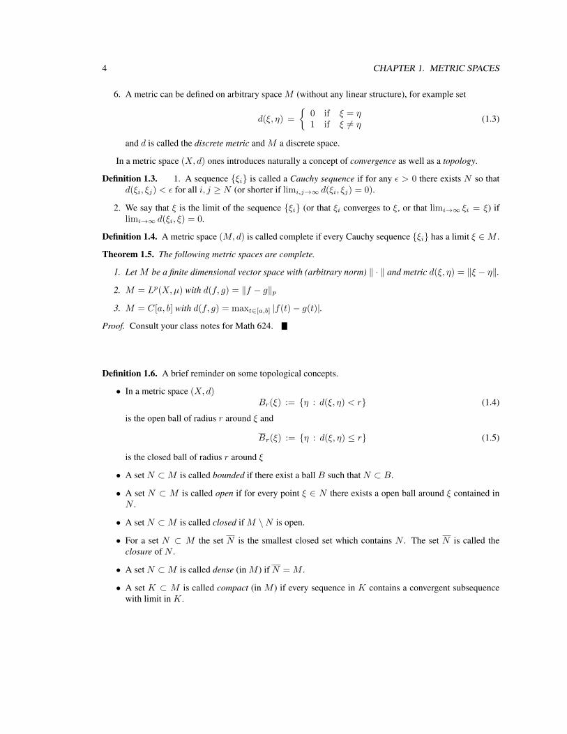
6. A metric can be defined on arbitrary space M (without any linear structure), for example set
d(ξ, η) =
0 if ξ = η1 if ξ 6= η
(1.3)
and d is called the discrete metric and M a discrete space.
In a metric space (X, d) ones introduces naturally a concept of convergence as well as a topology.
Definition 1.3. 1. A sequence ξi is called a Cauchy sequence if for any ε > 0 there exists N so thatd(ξi, ξj) < ε for all i, j ≥ N (or shorter if limi,j→∞ d(ξi, ξj) = 0).
2. We say that ξ is the limit of the sequence ξi (or that ξi converges to ξ, or that limi→∞ ξi = ξ) iflimi→∞ d(ξi, ξ) = 0.
Definition 1.4. A metric space (M,d) is called complete if every Cauchy sequence ξi has a limit ξ ∈M .
Theorem 1.5. The following metric spaces are complete.
1. Let M be a finite dimensional vector space with (arbitrary norm) ‖ · ‖ and metric d(ξ, η) = ‖ξ − η‖.
2. M = Lp(X,µ) with d(f, g) = ‖f − g‖p
3. M = C[a, b] with d(f, g) = maxt∈[a,b] |f(t)− g(t)|.
Proof. Consult your class notes for Math 624.
Definition 1.6. A brief reminder on some topological concepts.
• In a metric space (X, d)Br(ξ) := η : d(ξ, η) < r (1.4)
is the open ball of radius r around ξ and
Br(ξ) := η : d(ξ, η) ≤ r (1.5)
is the closed ball of radius r around ξ
• A set N ⊂M is called bounded if there exist a ball B such that N ⊂ B.
• A set N ⊂ M is called open if for every point ξ ∈ N there exists a open ball around ξ contained inN .
• A set N ⊂M is called closed if M \N is open.
• For a set N ⊂ M the set N is the smallest closed set which contains N . The set N is called theclosure of N .
• A set N ⊂M is called dense (in M ) if N = M .
• A set K ⊂ M is called compact (in M ) if every sequence in K contains a convergent subsequencewith limit in K.
1.2. BANACH FIXED POINT THEOREM 5
1.2 Banach fixed point theoremProblem 1.7. As a motivation imagine we want to solve the fixed point problem
F (ξ) = ξ (1.6)
where F : M →M is some map (not necessarily linear).
The idea of the solution is simple. Pick a point ξ0 and define the sequence ξn inductively by
ξn+1 = F (ξn) . (1.7)
If this sequence converges to ξ and F is continuous we have then
ξ = limn→∞
ξn+1 = limn→∞
F (ξn) = F ( limn→∞
ξn) = F (ξ) (1.8)
and so ξ is a solution of the fixed point problem.We have the following
Theorem 1.8. (Banach Fixed Point Theorem) Let (M,d) be a complete metric space and let F : M →Mbe a contraction, i.e., there exists q ∈ [0, 1) such that for all ξ, η ∈M
d(F (ξ), F (η)) ≤ qd(ξ, η) . (1.9)
Then F has exactly one fixed point ξ = limn Fn(ξ0) for arbitrary ξ0.
Proof. We haved(ξn+1, ξn) ≤ qd(F (ξn), F (ξn−1)) ≤ · · · ≤ qnd(ξ1, ξ0) . (1.10)
Using that q < 1 we have then
d(ξn+m, ξn) ≤m∑k=1
d(ξn+k, ξn+k−1)
≤m∑k=1
qn+k−1d(ξ1, ξ0)
≤ qn
1− qd(ξ1, ξ0) . (1.11)
Since (M,d) is complete, ξ = limn→∞ ξn exists.To show that ξ is a fixed point we note that
Example 1.9. Let us try to solve the set of linear equation
n∑i=1
aikxk = zk (1.14)
where zk, k = 1, · · · , n are given and xk, k = 1, · · · , n are unknown. We rewrite it as a fixed point equation
xi =
n∑k=1
(aik + δik)xk − zi (1.15)
orξ = F (ξ) (1.16)
where ξ = (x1, · · · , xn) ∈ Rn (or Cn) and
F (ξ) = Cξ + ζ (1.17)
where ζ = (z1, · · · , zn) and C is the matrix with cik = aik + δik.To apply the Banach fixed point theorem we pick a metric on Cn such that (Cn, d) is complete. For
example we can take d(ξ, η) = ‖ξ − η‖p with p ≥ 1 and then we have
d(F (ξ), F (η)) = ‖C(ξ − η)‖p (1.18)
For example if p = 1 we have
‖Cξ‖1 =∑i
∣∣∣∣∣∑k
cikxk
∣∣∣∣∣ ≤ ∑i
∑k
|cik||xk| ≤ maxk
∑I
|cik|︸ ︷︷ ︸:=q1
‖ξ‖1 . (1.19)
If we can find a norm such that ‖C(ξ)‖ ≤ q‖ξ‖ then the equation (1.9) has a unique solution.The fixed point equation has the form ξ = Cξ + ζ or (1 − C)ξ = ζ which gives formally using a
Neumann series (which we will justify later)
ξ = (1− C)−1ζ = (1 + C + C2 + · · · )ζ . (1.20)
Note also that the Banach fixed point algorithms gives the sequence
ξn+1 = Cξn + ζ (1.21)
and ξ is the limit of ξn independent of the starting point ξ0. This iteration is easy to solve and gives
ξn = Cnξ0 +
n−1∑k=1
Ckζ (1.22)
and thus, formally, we find
ξ = limn→∞
Cnξ0 +
∞∑k=1
Ckζ (1.23)
The second term is exactly the Neumann series and the first term should go to 0.
1.2. BANACH FIXED POINT THEOREM 7
Example 1.10. (Fredholm integral equation) A very similar argument applies to the equation
f(t) = λ
∫ b
a
k(t, s)f(s) ds+ h(t) (1.24)
where we use the metric space C[a, b] with the maximum metric d(f, g) =∫ ba|f(t) − g(t)|dt. This is a
fixed point equation f = F (f) where
F (f)(t) = h(t) + λ
∫ b
a
k(t, s)f(s) ds . (1.25)
We have
d(F (f), F (g)) = maxt∈[a,b]
|F (f)(t)− F (g)(t)| = maxt∈[a,b]
∣∣∣∣∣∫ b
a
λk(t, s)(f(s)− g(s)) ds
∣∣∣∣∣≤ |λ|
(maxt∈[a,b]
∫ b
a
|k(t, s)| ds
)d(f, g) . (1.26)
From the Banach fixed point theorem we deduce that the Fredholm integral equation has a unique solutionprovided
|λ| ≤
(maxt∈[a,b]
∫ b
a
|k(t, s)| ds
)−1
(1.27)
Example 1.11. (Solving differential equations) Consider an ordinary differential equation (initial valueproblem)
dx(t)
dt= f(x(t)) , x(a) = x0 (1.28)
where f : R→ R. It is easy to see that x(t) is solution of (1.28) on the interval [a, b] if and only if we havefor t ∈ [a, b]
x(t) = x0 +
∫ t
a
f(x(s)) ds , a ≤ t ≤ b . (1.29)
We can interpret this equation as a fixed point equation in M = x ∈ C[a, b] : x(0) = x0 which is aclosed subspace of a Banach space and thus itself a Banach space. We define F : M →M ] by
F (x)(t) = x0 +
∫ t
a
f(x(s)) ds , a ≤ t ≤ b (1.30)
and thus x(t) is a solution of (1.28) on the interval [a, b] if and only if F (x)(t) = x(t) for t ∈ [a, b].In order to apply the Banach fixed point theorem we assume that f is globally Lipschitz, i.e., there exists
a constant L > 0 such that for all x, y ∈ R
|f(x)− f(y)| ≤ L|x− y| (1.31)
Then if we equip C[a, b] with the maximum metric we have
d(F (x), F (y)) = supt∈[a,b]
|F (x(t))− F (y(t))| ≤ supt∈[a,b]
∫ t
a
|f(x(s))− f(y(s))| ds
≤ L
∫ t
a
|x(s)− y(s)| ≤ L(b− a) d(x, y) . (1.32)
8 CHAPTER 1. METRIC SPACES
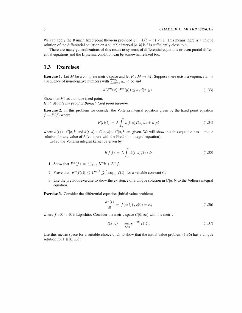
We can apply the Banach fixed point theorem provided q = L(b − a) < 1. This means there is a uniquesolution of the differential equation on a suitable interval [a, b] is b is sufficiently close to a.
There are many generalizations of this result to systems of differential equations or even partial differ-ential equations and the Lipschitz condition can be somewhat relaxed too.
1.3 ExercisesExercise 1. Let M be a complete metric space and let F : M 7→M . Suppose there exists a sequence an isa sequence of non-negative numbers with
∑∞n=1 an <∞ and
d(Fn(x), Fn(y)) ≤ and(x, y) . (1.33)
Show that F has a unique fixed point.Hint: Modify the proof of Banach fixed point theorem
Exercise 2. In this problem we consider the Volterra integral equation given by the fixed point equationf = F (f) where
F (t)(t) = λ
∫ t
a
k(t, s)f(s) ds+ h(s) (1.34)
where h(t) ∈ C[a, b] and k(t, s) ∈ C[a, b]×C[a, b] are given. We will show that this equation has a uniquesolution for any value of λ (compare with the Fredholm integral equation).
Let K the Volterra integral kernel be given by
Kf(t) = λ
∫ t
a
k(t, s)f(s) ds (1.35)
1. Show that Fn(f) =∑nk=0K
kh+Knf .
2. Prove that |Knf(t)| ≤ Cn (t−a)n
n! supt |f(t)| for a suitable constant C.
3. Use the previous exercise to show the existence of a unique solution in C[a, b] to the Volterra integralequation.
Exercise 3. Consider the differential equation (initial value problem)
dx(t)
dt= f(x(t)) , x(0) = x0 (1.36)
where f : R→ R is Lipschitz. Consider the metric space C[0,∞) with the metric
d(x, y) = supt≥0
e−Dt|f(t)| . (1.37)
Use this metric space for a suitable choice of D to show that the initial value problem (1.36) has a uniquesolution for t ∈ [0,∞).
Chapter 2
Normed Vector Spaces
For general metric spaces (M,d) the set M has no structure besides the topology induced buy the norm. Weconcentrate now on the special case where
M = V = vector space over K with K = R or C
2.1 Some concepts from linear algebraWe recall some basic concepts from linear algebra slightly generalized to vector spaces which may haveinfinite dimension. In this section we do not use any topological concepts yet.
Definition 2.1. 1. A set M ⊂ V is called linearly independent if every finite subset of M is linearlyindependent.
2. The set E ⊂ V is called a Hamel basis (algebraic basis) of V if E is linearly independent and everyvector ξ ∈ V can be written uniquely as finite linear combination of elements in E.
Using Zorn’s Lemma one can prove that
Theorem 2.2. Let M ⊂ V be linearly independent. Then V has a Hamel basis which contains M .
We use the following notations: for N,M ⊂ V , ξ ∈ V and a ∈ K
ξ +M = ξ + η ; η ∈M ,N +M = ξ + η ; ξ ∈ N, η ∈M ,
aM = aξ ; ξ ∈M .
Definition 2.3. 1. If M and N are subspaces of V and M ∩ N = 0 then M + N is a subspace andone write M +N as M ⊕N (direct sum).
2. If V = M ⊕N we say that M and N are complementary subspaces.
Proposition 2.4. To each subspace M ⊂ V there exists a complementary subspace N (not uniquely de-fined).
9
10 CHAPTER 2. NORMED VECTOR SPACES
Proof. LetEM a Hamel basis ofM andE a Hamel basis of V which containsEM (see the proof of Theorem2.2). Then E \ EM generates a subspace N which is complementary to M .
Definition 2.5. If V = M ⊕N and dimN = n <∞ then we say that M has codimension n, i.e.,
codimM = dimM . (2.1)
One check easily that
Proposition 2.6. If V = M ⊕N1 = M ⊕N2. Then dimN1 = dimN2.
Definition 2.7. Suppose V = M ⊕N . Then any ξ ∈ V has a unique decomposition
ξ = α+ β (2.2)
with α ∈M , β ∈ N . The projection of ξ on M along N is given by
Pξ = α . (2.3)
One verifies easily that
Lemma 2.8. We have P 2 = P .
Conversely we have
Lemma 2.9. Suppose P : V → V is linear map such that P 2 = P . Then V = M ⊕N where M = PVand N = (1− P )V .
Proof. For any ξ ∈ V we haveξ = Pξ︸︷︷︸
∈M
+ (1− P )ξ︸ ︷︷ ︸∈N
(2.4)
and thus V = M +N . The sum is direct, since if
ξ ∈M ∩N = PV ∩ (1− P )V (2.5)
we have, on one hand, ξ = Pα and so
Pξ = P 2α = Pα = ξ . (2.6)
On the other hand ξ = (1− P )β and so we obtain
ξ = Pξ = P (1− P )β = (P − P 2)β = 0 . (2.7)
Thus M ∩N = 0.
Using projections we can prove
Theorem 2.10. Suppose T : V → W is a linear map. Let P a projection on the nullspace of T and Q aprojection along the range of T . Then there exists a linear map S : W → V such that
ST = 1V − P , TS = 1W −Q . (2.8)
The map T is bijective if and only P = Q = 0.
2.2. NORM 11
Proof. Let us denote N = N (T ) ⊂ V the nullspace (or kernel) of T and and M = R(T ) ⊂ W the rangeof T . We have
V = N ⊕ V1 , W = W1 ⊕M . (2.9)
and P is the projection on N along V1 and Q the projection on W1 along M .We define T0 : V1 →M by T0ξ = Tξ. Then T0 is bijective and so T−1
0 : M → V1 exists. If
S = T−10 (1−Q) : W → V1 (2.10)
we have
STξ =
0 if ξ ∈ Vξ if ξ ∈ V1
(2.11)
and soST = 1V − P . (2.12)
Arguing similarly we haveTS = 1W −Q . (2.13)
2.2 NormSuppose we have a metric d on a vector space V . It is natural to ask whether the metric respects the linearstructure of V . By that we mean that
1. d is translation invariant, i.e., d(ξ + α, η + α) = d(ξ, η) for all α ∈ V .
2. Under scalar multiplication we have d(aξ, aη) = |a|d(ξ, η).
Property 1. implies that d(ξ, η) = d(ξ−η, 0). If we set then ‖ξ‖ := d(ξ, 0) we have then from the propertiesof the distance that
(N1) ‖ξ‖ ≥ 0 and ξ = 0 if and only if ξ = 0.
(N2’) ‖ξ‖ = ‖ − ξ‖ (symmetry)
(N3) ‖ξ + η‖ ≤ ‖ξ‖+ ‖η‖
while from Property 2., instead of (N2’) we obtain the stronger
(N2) ‖aξ‖ = |a|‖ξ‖
Definition 2.11. (Normed vector spaces)
1. A map ‖ · ‖ : V → R is called a norm on V if it satisfies the condition (N1), (N2), and (N3).
2. The pair (V, ‖ · ‖) is called a normed vector space.
3. A complete normed vector space is called a Banach space.
Note that in a normed vector space we have convergence in the sense of the metric defined by d(ξ, η) =‖ξ − η‖ or equivalently ξn converges to ξ if and only if limn→∞ ‖ξ − ξn‖ = 0.
12 CHAPTER 2. NORMED VECTOR SPACES
Example 2.12. We give examples of normed vector spaces (see Math 623-624 for details and proofs).
1. For p ≥ 1,
lp =ξ = (x1, x2, x3, · · · )xi ∈ C with ‖ξ‖p := (
∑i
|xi|p)1/p <∞
(2.14)
is a Banach space. The completeness is non-trivial as is the triangle inequality (a.k.a Minkowskyinequality).
2. The spacel∞ =
ξ = (x1, x2, x3, · · · )xi ∈ C with ‖ξ‖∞ := sup
i|xi| <∞
(2.15)
is a Banach space as well as
c0 =ξ ∈ l∞ , ξ = (x1, x2, x3, · · · ) lim
ixi = 0
(2.16)
andc =
ξ ∈ l∞ , ξ = (x1, x2, x3, · · · ) lim
ixi exists
(2.17)
3. The space
Cn[a, b] =f : [a, b]→ R : f n times continuously differentiable
(2.18)
is a Banach space with the norm
‖f‖ =
n∑k=0
maxt∈[a,b]
|f (k)(t)| (2.19)
where f (k) is the k-th derivetive of f .
4. The spaceBV [a, b] =
f : [a, b]→ R : f of bounded variation
(2.20)
is a Banach space with the norm‖f‖ = |f(a)|+ V (f) (2.21)
where V (f) is the variation of f on [a, b] given by
V (f) = supP
N∑k=1
|f(xk)− f(xk−1| (2.22)
where P is set of partition of [a, b]: a = x0 < x1 < · · · < xn = b.
The following facts are very easy but also very important
Proposition 2.13. Let (V, ‖ · ‖) be a normed vector space.
1. The linear operations are continuous
2. The map ξ → ‖ξ‖ is continuous.
2.3. CONTINUOUS LINEAR MAPS 13
Proof. If ξn → ξ and ηn → η then ξn + tηn → ξ + tη since
If ξn → ξ then ‖ξn‖ → ‖ξ‖ since|‖ξ‖ − ‖ξn‖| ≤ ‖ξ − ξn‖ (2.24)
by the (reverse) triangle inequality.
Definition 2.14. (Comparison of norms) Suppose two norms ‖ · ‖1 and ‖ · ‖2 are given on a vector spaceV .
1. The norm ‖ · ‖1 is stronger than ‖ · ‖2 if there exists C > 0 such that for all ξ ∈ V .
‖ξ‖2 ≤ C‖ξ‖1 (2.25)
2. The The norms ‖ · ‖1 and ‖ · ‖2 are equivalent if there exists constants C and D such that
D‖ξ1‖ ≤ ‖ξ‖2 ≤ C‖ξ‖1 . (2.26)
Clearly equivalent norm induce the same topology since convergence of one sequence in one normimplies the convergence of the sequence in the other norm.
Theorem 2.15. If dim(V ) <∞ then all norms on V are equivalent.
Proof. : This is left as an exercise. Use Bolzano-Weierstrass.
2.3 Continuous linear mapsLet (V, ‖ · ‖V ) and (W, ‖ · ‖W ) be two normed vector space. In the sequel, whenever there is no risk ofconfusion we shall drop the index V or W from the norm and simply denote it by ‖ · ‖. We also consider alinear map
T : V →W . (2.27)
Unless explicitly specified we will deal only with linear maps in the sequel. We also use the notation Tξ forT (ξ)
Definition 2.16. Let T : V →W be a linear map.
1. The map T is bounded if there exists a constant C ≥ 0 such that
‖Tξ‖ ≤ C‖ξ‖ (2.28)
for all ξ ∈ V .
2. The norm of T , denoted by ‖T‖ is the smallest C such that (2.28) holds, i.e.
‖T‖ := supξ∈V,ξ 6=0
‖Tξ‖‖ξ‖
= supξ∈V,‖ξ‖=1
‖Tξ‖ . (2.29)
14 CHAPTER 2. NORMED VECTOR SPACES
3. The set of bounded linear maps is denoted by
L(V,W ) =T : V →W, T linear and bounded
(2.30)
and we writeL(V ) := L(V, V ) . (2.31)
Theorem 2.17. Let T be a linear map. Then T is bounded if and only if T is continuous.
Proof. Suppose T is bounded, then we have
‖Tξ − T η‖ = ‖T (ξ − η)‖ ≤ ‖T‖‖ξ − η‖ (2.32)
and this implies that T is (Lipschitz) continuous.Conversely let us assume that T is continuous but not bounded. Then there exists a sequence ξn such
that‖Tξn‖ ≥ n‖ξn‖ . (2.33)
Let us set
ηn =ξn√n‖ξn‖
.
Then we have
‖ηn‖ =1√n, ‖Tηn‖ > n‖ηn‖ =
√n . (2.34)
This means that ηn → 0 but Tηn is divergent which contradicts the continuity of T .
Example 2.18. Let us consider some examples of bounded (and not bounded operators). Many more exam-ples to come.
1. The identity operator 1 defined by 1ξ = ξ is bounded with ‖1‖ = 1.
2. The differentiation operator is not bounded. Take for example the space V which consists of polyno-mials p(t) on [0, 1] with the sup-norm and set Tp(t) = p′(t). Then if pn(t) = xn we have ‖pn‖ = 1for all n but ‖Tpn‖ = ‖ntn−1‖ = n and this shows that T is not bounded.
Note that differentiation is a very natural operation so to include it in our consideration we will con-sider unbounded linear operator later on.
3. The integral operator
Tf(t) =
∫ b
a
k(t, s)f(s) ds (2.35)
is bounded on C[a, b] equipped with the sup-norm if k(t, s) ∈ C([a, b] × [a, b]). Indeed we Tf(t) iscontinuous in t by e.g. the dominated convergence theorem and
‖Tf‖ = supt|∫ b
a
k(t, s)f(s) ds| ≤ sups|f(s)| sup
t
∫ b
a
|k(t, s)| ds︸ ︷︷ ︸≡C
(2.36)
2.3. CONTINUOUS LINEAR MAPS 15
and C is finite since k is continuous. Actually we can show that ‖T‖ = supt∫ ba|k(t, s)| ds. If
k(t, s) is nonnegative then we simply take f = 1 and we have ‖T1‖ = supt∫ ba|k(t, s)| ds. For a
general k we pick t0 such that supt∫ ba|k(t, s)| ds =
∫ ba|k(t0, s)| ds. Then we would like to pick
the function f(s) = sign k(t0, s) so that Tf(t0) =∫ bak(t0, s)f(s)ds =
∫ ba|k(t0, s)| ds. But this
f is not continuous and we need to use an approximation argument. Consider the function φn(t)which is piecewise linear, increasing, continuous, with φ(t) = sign t if |t| > 1/n. We set fn(s) =φn(k(t0, s)). We have
Tfn(t0) =
∫ b
a
k(t0, s)fn(s) ds =
∫ b
a
|k(t0, s)| ds−1
n(b− a) . (2.37)
From this it follows that ‖T‖ =∫ ba|k(t0, s)| ds.
4. The Fourier transform is defined by
f(k) =
∫Rf(x)e−i2πkx , (2.38)
and we write T (f) = f . In Math 623-624 ones proves (after some effort) that T : L1(R, dx) →C0(R) is a bounded operator with norm 1. Here C0(R) is the Banach space of continuous functionssuch that lim|x|→∞ |f(x)| → 0 equipped with the sup-norm. One also proves (after some moreeffort) that T : L2(R, dx) → L2(R, dx) defines an unitary transformation (i.e. T is invertible and‖Tf‖ = ‖f‖ for al f ).
Theorem 2.19. L(V,W ) is a normed vector space.
Proof. Let T , S ∈ V and a a scalar.
• (N1) We have ‖T‖ ≥ 0. If ‖T‖ = 0 then we have ‖Tξ‖ ≤ ‖T‖‖ξ‖ = 0 and so T = 0. Conversely ifT = 0 then obviously ‖T‖ = 0.
Theorem 2.20. If W is a Banach space then L(V,W ) is a Banach space.
Proof. Let Tn be Cauchy sequence in L(V,W ). For any ξ ∈ V we have
‖Tnξ − Tmξ‖ ≤ ‖Tn − Tm‖‖ξ‖ (2.39)
and thus Tnξ is a Cauchy sequence in W . Since W is complete this sequence has a limit in W and we set
η = limn→∞
Tnξ (2.40)
16 CHAPTER 2. NORMED VECTOR SPACES
We define then T : V → W by Tξ = η. The linearity of Tn immediately implies that T is linear. Whatremains to prove is that T is bounded and Tn → T . Given ε > 0 pick N such that for n,m > N we have
‖Tnξ − Tmξ‖ ≤ ‖Tn − Tm‖‖ξ‖ ≤ ε‖ξ‖ (2.41)
Using the continuity of the norm and taking m→∞ in (2.41) we have
‖Tnξ − Tξ‖ ≤ ε‖ξ‖ (2.42)
for any n ≥ N . This implies that ‖T − TN‖ ≤ ε and so ‖T‖ ≤ ‖T − TN‖ + ‖TN‖ < ∞ and so T isbounded. This also implies that ‖T − Tn‖ ≤ ε for n ≥ N and so Tn → T .
Theorem 2.21. For S ∈ L(U, V ) and T ∈ L(V,W ) we have TS := T S ∈ L(U,W ) and
‖TS‖ ≤ ‖T‖‖S‖ (2.43)
Proof. ‖TS‖ = sup‖ξ‖=1
‖TSξ‖ ≤ ‖T‖ sup‖ξ‖=1
‖Sξ‖ = ‖T‖‖S‖.
Corollary 2.22. For T ∈ L(V ) we have
1. ‖Tn‖ ≤ ‖T‖n
2. The limit r(T ) = limn→∞
‖Tn‖1/n exists and is called the spectral radius of T .
3. r(T ) = infn‖Tn‖1/n ≤ ‖T‖
Proof. 1. is immediate. For 2. and 3. set cn = ‖Tn‖/‖T‖n. Then we have 0 ≤ cn ≤ 1 and cn+m ≤ cncmand this implies that cn is a bounded decreasing sequence and so c = limn→∞cn exists. Therefore c1/nn isalso a decreasing with limit
limn→∞
‖Tn‖1/n
‖T‖= inf
n
‖Tn‖1/n
‖T‖(2.44)
The notation ”spectral radius” will become clear in the sequel.As an application we consider the Neumann series which is is a generalization of the geometric series.
Suppose V is a Banach space, T ∈ L(V ) with ‖T‖ = δ < 1. Then the series∑∞k=0 T
k converges sincesince the partial sum Sn =
∑∞k=0 T
k satisfy for n > m
‖Sn − Sm‖ ≤n∑
k=m+1
‖T k‖ ≤n∑
k=m+1
δk ≤ δm+1 1
1− δ(2.45)
and thus form a Cauchy sequence and we have limn Sn =∑k=0∞ T
k.Furthermore we have
(1− T )Sn = Sn(1− T ) = 1− Tn+1 → 1 (2.46)
and thus we conclude that 1− T is invertible and
(1− T )−1 =
∞∑k=0
T k . (2.47)
One can prove the stronger result
2.3. CONTINUOUS LINEAR MAPS 17
Theorem 2.23. Let V be a Banach space and T ∈ L(V ) with r(T ) < 1. Then (1 − T )−1 exists and isgiven by the Neumann series
(1− T )−1 =
∞∑k=0
T k (2.48)
Proof. Note first that∑TK converges whenever
∑k ‖T k‖ does. If r(T ) = δ < 1 then for any δ′ with
δ < δ′ < 1 there exists N such that for n > N we have ‖Tn‖1/n ≤ δ′. This means that ‖Tn‖ ≤ (δ′)n andso∑k ‖T k‖ converges. The rest is as before.
Linear operators occur naturally as derivative and this is true in infinite-dimensional spaces as well.
Definition 2.24. Let V and W be normed vector spaces and U ⊂ V open. The map F : U → W is said tobe differentiable at η ∈ U if there exists a continuous linear map F ′(a) such that
F (ξ) = F (η) + F ′(η)(ξ − η) +R(ξ)‖ξ − η‖ , (2.49)
where R : U →W satisfy limξ→η R(ξ) = 0.
Let is consider a few examples
Example 2.25. 1. Let V = W = C[a, b] and let k ∈ C[0, 1] × [0, 1] and g be twice continuouslydifferentiable. Let us consider the map
F (x)(t) =
∫ b
a
k(t, s)g(x(s)) ds (2.50)
To compute the derivative we pick h ∈ C[0, 1] and using the mean value theorem we obtain
F (x+ h)− F (x) =
∫ b
a
k(t, s) [g(x(s) + h(s))− g(x(s))] ds
=
∫ b
a
k(t, s)
[g′(x(s))h(s) +
1
2g′′(a(s))h(s)2
]ds (2.51)
where a(s) is a value between x(s) and x(s) + h(s). This computation shows that the linear F ′(x) :C[0, 1]→ C[0, 1] given by
F ′(x)(h)(t) =
∫ b
a
k(t, s)g′(x(s))h(s) ds (2.52)
is a good candidate for the derivative. Clearly this map is bounded since k(t, s)g′(x(s)) ∈ C[0, 1] ×[0, 1]. Moreover we have the bound
supt
∣∣∣∣∣∫ b
a
k1
2k(t, s)g′′(a(s))h(s)2 ds
∣∣∣∣∣ ≤ C‖h‖2 (2.53)
since g′′ is bounded by assumption. This shows that F is differentiable.
18 CHAPTER 2. NORMED VECTOR SPACES
2. Let E be a Banach space and consider the Banach space L(E). We say that T ∈ L(E) is an isomor-phism if T is linear, bijective, continuous and if A−1 is continuous. We will see in fact in Section 2.8that by the open map theorem the continuity of A−1 follows from the other assumptions.
In any case the setGL(E) = T ∈ L(E) : , T an isomorphism (2.54)
is an open subset of L(E). Indedd if T is an isomorphism then T + H is an isomorphism provided‖H‖ ≤ ‖T−1‖−1. This follows from T + H = T (1 + T−1H), from ‖T−1H‖ ≤ ‖T−1‖‖H‖ < 1and from the geometric series.
Let us consider the map F : GL(E)→ L(E) given by
F (T ) = T−1 . (2.55)
We claim that the F is differentiable and that we have
F ′(T )H = −T−1HT−1 . (2.56)
The continuity of F ′(T ) is clear since we have ‖F ′(T )H‖ ≤ ‖A−1‖2‖H‖. Furthermore we have
F (T +H)− F (T ) = (T +H)−1 − T−1 =[(1 + T−1H)− 1
]T−1
=
∞∑j=1
(−T−1H)jT−1 (2.57)
if ‖H‖ ≤ ‖T−1‖−1 (geometric series). The first term in the series is −T−1HT−1 and the remaindercan be bounded by ‖T−1‖2‖H‖(1 − ‖T−1‖‖H‖)−1. The reminder divided by ‖H‖ tends to 0,showing the differentiability.
Pointwise (strong) convergence: In L(V,W ), in addition to norm convergence ( ≡ uniform convergence)there is the weaker notion of point wise convergence.
Definition 2.26. Let Tn a sequence in L(V,W ) and T ∈ L(V,W ). We say that Tn converges strongly toT and write
T = s− limn→∞
Tn (2.58)
if for any ξ ∈ V we havelimn→∞
Tnξ = Tξ . (2.59)
Whenever we need to differentiate between different types of convergence we will write n− limn→∞ Tnfor the convergence in norm.
The following two lemmas are very easy and the proof is left to the reader.
Lemma 2.27. If n− limn→∞ Tn = T then s− limn→∞ Tn = T .
Lemma 2.28. The linear operations are continuous with respect to strong convergence.
However note that if n − limn→∞ Tn = T then Tn‖ → ‖T‖ but this does not necessarily hold in thecase of strong convergence. Similarly if n − limn→∞ Tn = T and n − limn→∞ Sn = S then we haven− limn→∞ SnTn = ST but this does not necessarily hold for strong convergence.
2.4. LINEAR FUNCTIONALS AND DUAL SPACES 19
Example 2.29. Let V = lp and for ξ = (x1, x2, · · · ) let us set
Tnξ = (x1, · · · , xn, 0, 0, · · · ) . (2.60)
Then we have Tnξ − ξ → 0 and so s− limn→∞ Tn = 1. But since
for any n we can find ηn with ‖ηn = 1‖ = 1 and (1− Tn)ηn = ηn. This implies that ‖1− Tn‖ = 1 for alln and so n− limn→∞ Tn is certainly not equal to 1.
2.4 Linear functionals and dual spacesDefinition 2.30. If V is a Banach space over K = R or C then L(V,K) is a Banach space. We write
V ′ := L(V,K) (2.62)
and V ′ is called the dual space. The elements of V ′ are called linear functionals on V and for λ ∈ V ′ thenorm is given by
‖λ‖ = supξ∈V‖ξ‖=1
|λ(ξ)| . (2.63)
Let us work out an example in detail
Example 2.31. If V = lp for p > 1 then V ′ = lq where p−1 + q−1 = 1.
Proof. Note first that if η = (y1, y2, · · · ) ∈ lq then λη(ξ) defined by
λη(ξ) =
∞∑k=1
xkyk (2.64)
defines a bounded linear functional on lp since by Holder’s inequality we have
|λη(ξ)| ≤ ‖ξ‖p‖η‖q , (2.65)
and so ‖λη‖ ≤ ‖η‖q .Let us denote
εk = δik∞i=1 ∈ lp . (2.66)
Any ξ ∈ lp can be written as the convergent series in lp
ξ =
∞∑k=1
xkεk . (2.67)
Let λ ∈ V , since it is continuous, we have
λ(ξ) =∑k
xkyk with yk = λ(εk) . (2.68)
and we set η = yk and λ has the from λη .
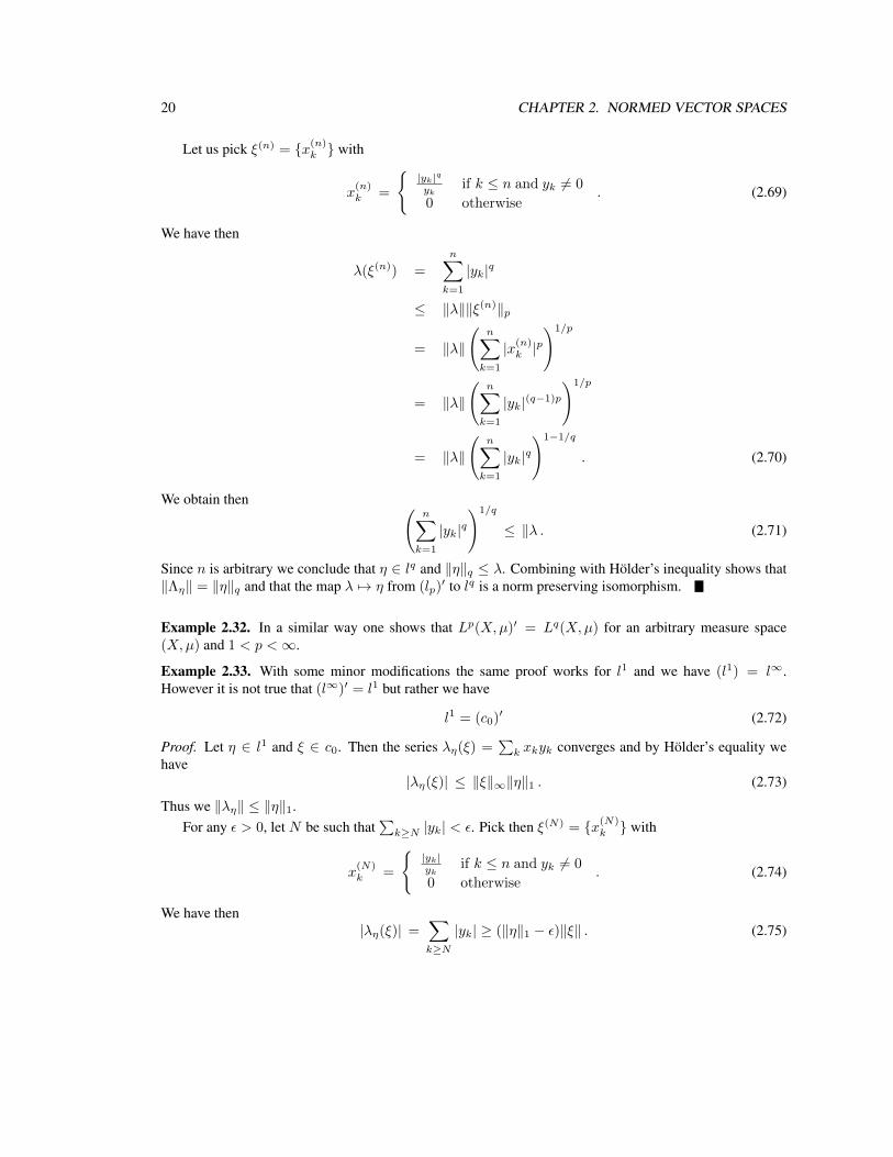
20 CHAPTER 2. NORMED VECTOR SPACES
Let us pick ξ(n) = x(n)k with
x(n)k =
|yk|qyk
if k ≤ n and yk 6= 0
0 otherwise. (2.69)
We have then
λ(ξ(n)) =
n∑k=1
|yk|q
≤ ‖λ‖‖ξ(n)‖p
= ‖λ‖
(n∑k=1
|x(n)k |
p
)1/p
= ‖λ‖
(n∑k=1
|yk|(q−1)p
)1/p
= ‖λ‖
(n∑k=1
|yk|q)1−1/q
. (2.70)
We obtain then (n∑k=1
|yk|q)1/q
≤ ‖λ . (2.71)
Since n is arbitrary we conclude that η ∈ lq and ‖η‖q ≤ λ. Combining with Holder’s inequality shows that‖Λη‖ = ‖η‖q and that the map λ 7→ η from (lp)
′ to lq is a norm preserving isomorphism.
Example 2.32. In a similar way one shows that Lp(X,µ)′ = Lq(X,µ) for an arbitrary measure space(X,µ) and 1 < p <∞.
Example 2.33. With some minor modifications the same proof works for l1 and we have (l1) = l∞.However it is not true that (l∞)′ = l1 but rather we have
l1 = (c0)′ (2.72)
Proof. Let η ∈ l1 and ξ ∈ c0. Then the series λη(ξ) =∑k xkyk converges and by Holder’s equality we
have|λη(ξ)| ≤ ‖ξ‖∞‖η‖1 . (2.73)
Thus we ‖λη‖ ≤ ‖η‖1.For any ε > 0, let N be such that
∑k≥N |yk| < ε. Pick then ξ(N) = x(N)
k with
x(N)k =
|yk|yk
if k ≤ n and yk 6= 0
0 otherwise. (2.74)
We have then|λη(ξ)| =
∑k≥N
|yk| ≥ (‖η‖1 − ε)‖ξ‖ . (2.75)
2.5. HAHN-BANACH THEOREM 21
Therefore ‖λη‖ ≥ ‖η‖1 and so ‖λη‖ = ‖η‖1.It remains to show that every linear functional on c0 has the above form. If ξ ∈ c0 then we can write
ξ =∑∞k=1 xkεk (not true in l∞!) and so for any λ ∈ c′0 there exists η = yk such that λ(ξ) = λη(ξ) =∑∞
k=1 xkyk. Picking ξ(n) as in (2.74) we have ‖ξ(n)‖∞ = 1 and
‖λη(ξ(n)) =
(n∑k=1
|yk|
)‖ξ(n)‖∞ (2.76)
from which we conclude that ‖λη‖ ≥ ‖η‖1, i.e. η ∈ l1.
Schauder basis and separability:
Definition 2.34. A metric space is called separable if it contains a countable dense set.
One shows that lp is separable but l∞ is not separable.
In the construction of dual spaces we used the fact that any ξ ∈ lp, 1 ≤ p < ∞ can be written uniquelyas
ξ =∑k=1
xkεk , with ‖ξ‖p =
(∑k=1
|xk|p)1/p
<∞ (2.77)
In general we have
Definition 2.35. A countable subset B = εk of a normed vector space V is called a Schauder Basis of Vif each vector ξ ∈ V can be written uniquely as ξ =
∑∞k=1 xkεk.
Without difficulty one shows that
Lemma 2.36. A normed vector space which has a Schauder basis is separable.
It is a remarkable and deep fact that the converse does not hold: there exists Banach spaces which areseparable but do not have a Schauder basis. (See P. Enflo. A counterexample to the approximation problemin Banach spaces, Acta Math 130, 309, (1973).)
2.5 Hahn-Banach theoremAs we will see a very important question in functional analysis is how to extend a functional defined on asubspace W of a vector space V to all V while respecting some properties.
Theorem 2.37. Hahn-Banach (real vector spaces) Let V a vector space over R and p : V → R a convexfunction on V , i.e. we have
p(aξ + (1− a)η) ≤ ap(ξ) + (1− a)p(η) (2.78)
for any a ∈ [0, 1] and all ξ, η ∈ V .
22 CHAPTER 2. NORMED VECTOR SPACES
Let φ be a linear functional defined on the subspace W ⊂ V such that we have
φ(ξ) ≤ p(ξ) for all ξ ∈W . (2.79)
Then there exists a linear functional Φ defined on V such that
Φ(ξ) = φ(ξ) for all ξ ∈W .
Φ(ξ) ≤ p(ξ) for all ξ ∈ V . (2.80)
A very important example of a convex function p is a norm (or a semi-norm) on V , i.e., p(ξ) = ‖ξ‖.
Proof. The idea of the proof is to show that one can extend φ from W to W + Rη for any ξ /∈ W . The restfollows from an applications of Zorn’s lemma.
Let us choose η /∈ W and let denote W1 = W + Rη. By linearity it is enough to specify c := φ(η) todefine an extension φ1 on W1 since we have then
φ1(ξ + aη) = φ1(ξ) + aφ1(η) = φ(ξ) + ac . (2.81)
To obtain the desired bound on φ1 we need that for all ξ ∈W and a ∈ R we must have
φ1(ξ + aη) = φ(ξ) + ac ≤ p(ξ + aη) . (2.82)
We restrict ourselves to a > 0. Then we looking for a c such that
φ(ξ) + ac ≤ p(ξ + aη)
φ(ξ)− ac ≤ p(ξ − aη)
or
c ≤ 1
a(p(ξ + aη)− φ(ξ))
c ≥ 1
a(−p(ξ − aη) + φ(ξ))
(2.83)
Such a c exists provided we can prove that
supξ∈W ,a>0
1
a(−p(ξ − aη) + φ(ξ)) ≤ inf
ξ∈W ,a>0
1
a(p(ξ + aη)− φ(ξ)) (2.84)
that is1
a1(−p(ξ1 − a1η) + φ(ξ1)) ≤ 1
a2(p(ξ2 + a2η)− φ(ξ2)) (2.85)
for all a1, a2 ≥ 0 and ξ1, ξ2 ∈W . Since a1 and a2 are non-negative this is equivalent to
This is exactly (2.86) and thus we have proved the existence of c := φ1(η).We now use Zorn’s lemma. Let A the set of all extension ψ won φ auf some subspace Wψ with the
property that φ = ψ on W and ψ(ξ) ≤ p(ξ) for all ξ ∈ Wψ . In A we can define a partial ordering throughψ1 ≺ ψ1 if Wψ1
⊂ Wψ2and ψ1 = ψ2 on Wψ1
. Suppose B ⊂ A is totally ordered and define then Ψon ∪ψ∈BWψ through Ψ(ξ) = ψ(ξ) on Wψ . By construction ψ ≺ Ψ for all ψ ∈ B and so B has an upperbound. By Zorn’s lemmaA has a maximal element Φ which satisfies Φ = φ onW and Φ(ξ) ≤ p(ξ). FinallyWΦ must be V since otherwise one could extend Φ as before and this contradicts maximality.
This theorem as an extension to complex vector spaces.
Theorem 2.38. Hahn-Banach (real vector spaces) Let V a vector space over C and p : V → R such thatwe have p(aξ + bη) ≤ |a|p(ξ) + |b|p(η) for any a, b ∈ C with |a|+ |b| = 1 and all ξ, η ∈ V .
Let φ be a complex linear functional defined on the subspace W ⊂ V such that we have
|φ(ξ)| ≤ p(ξ) for all ξ ∈W . (2.88)
Then there exists a linear functional Φ defined on V such that
Φ(ξ) = φ(ξ) for all ξ ∈W .
|Φ(ξ)| ≤ p(ξ) for all ξ ∈ V . (2.89)
Proof. The functional φr(ξ) = Reφ(ξ) is a real functional on V viewed as a vector field over R. In addition
φr(iξ) = Reφ(iξ) = Reiφ(ξ) = −Imφ(ξ) . (2.90)
and soφ(ξ) = φr(ξ)− iφr(iξ) . (2.91)
Conversely given any real linear functional Φr on V let us define Φ(ξ) = Φr(ξ) − iΦr(iξ). It is certainlylinear over R and we have
It is hard to overemphasize how important this theorem is for the foundations of functional analysis. Letus first derive some corollaries and then discuss a number of applications.
Corollary 2.39. Let (V, ‖ ·‖) be a normed vector space, W ⊂ V a subspace, and φ ∈W ′. Then there existsλ ∈ V ′ such that λ = φ on W and ‖λ‖ = ‖φ‖.
Proof. Take p(ξ) = ‖φ‖‖ξ‖ and apply Hahn-Banach.
Corollary 2.40. Let (V, ‖ · ‖) be a normed vector space, 0 6= ξ ∈ V . Then there exists λ ∈ V ′ such thatλ(ξ) = ‖ξ‖ and ‖λ‖ = 1.
Proof. Let W = Kξ be the subpsace spanned by ξ and set φ(aξ) = a‖ξ‖. This is a linear functional with‖φ‖ = 1. Now use Corollary 2.39.
Corollary 2.41. Let (V, ‖ · ‖) be a normed vector space, W ⊂ V a subspace. Let ξ ∈ V be such that
infη∈W
‖ξ − η‖ = δ > 0 . (2.94)
Then there exists λ ∈ V ′ such that ‖λ‖ = 1, λ(ξ) = δ and λ(η) = 0 for η ∈W .
Proof. Consider the subspace W1 = W ⊕Kξ and let define λ1 on W1 by
λ1(η + aξ) = aδ (2.95)
Clearly we have λ1(η) = 0 for η ∈ W and λ1(ξ) = δ. The functional λ1 is linear and bounded with norm1: using the assumption (2.94) we have
‖η + aξ‖ = ‖ − a(−1
aη − ξ)‖ = |a|‖ − 1
aη − ξ‖ ≥ |a|δ = |λ1(η + aξ)‖ (2.96)
and so ‖λ1‖ ≤ 1. On the other hand for ε > 0 there exists η ∈W such that
δ ≤ ‖ξ − η‖ ≤ δ(1 + ε) . (2.97)
Then we have
λ1(ξ − η) = δ ≥ 1
1 + ε‖ξ − η‖ , (2.98)
that is ‖λ1‖ ≥ (1 + ε)−1. So ‖λ1‖ = 1. Now use Corollary 2.39 for any ‖ξ‖ there exists
2.6. APPLICATIONS OF HAHN-BANACH THEOREM 25
2.6 Applications of Hahn-Banach theorem
Dual and bidual spaces The Hahn-Banach space is useful to derive the properties of the dual space V ′ aswell as the bidual V ′′ = (V ′)′ of a Banach space. First we derive a dual representation of the norm
Theorem 2.42. Let V be a normed vector space. Then we have
‖ξ‖ = supλ∈V ′ ,λ6=0
|λ(ξ)|‖λ‖
(2.99)
In particular if ξ0 is such that λ(ξ0) = 0 for all λ ∈ V ′ then ξ0 = 0.
Proof. On one hand from |λ(ξ)| ≤ ‖λ‖‖ξ‖ we have
‖ξ‖ ≥ supλ∈V ′ ,λ6=0
|λ(ξ)|‖λ‖
. (2.100)
Using corollary 2.40 for a given fixed ξ there exists λξ ∈ V ′ such that ‖λ‖ = 1 and
‖ξ‖ = λξ(ξ) =|λξ(ξ)|‖λξ‖
. (2.101)
The next results describe the relation between a Banach space V and his bidual V ′′.
Theorem 2.43. Let V be a normed vector space. For ξ ∈ V define an element ξ ∈ V ′′ by
ξ(λ) = λ(ξ) , λ ∈ V ′ . (2.102)
Then the map
J : V → V ′′
ξ 7→ ξ (2.103)
is an isometric isomorphism from V to a subspace of V ′′.
Proof. Since |ξ(λ)| = |λ(ξ)| ≤ ‖λ‖V ′‖ξ‖V is ξ a bounded linear functional on V ′ with
‖ξ‖V ′′ ≤ ‖ξ‖V . (2.104)
This shows that J(V ) ⊂ V ′′ and it remains to show that ‖ξ‖V ′′ = ‖ξ‖V . By corollary 2.40 given ξ thereexists λξ ∈ V ′ such that λξ(ξ) = ‖ξ‖. Then we have
‖ξ‖V ′′ = supλ∈V ′,‖λ‖=1
|ξ(λ)| ≥ |ξ(λξ)| = λξ(ξ) = ‖ξ‖V . (2.105)
Therefore J is an isometry of V onto its range.
The following theorem suggest
26 CHAPTER 2. NORMED VECTOR SPACES
Definition 2.44. A Banach space V is called reflexive (or self-dual) if J : V → V ′′ is bijective.
With respect to separability we have
Theorem 2.45. A normed vector space V is separable if V ′ is separable.
Proof. Consider a dense set λkk≥1 in V ′ and for each k pick ξk ∈ V with ‖ξk‖ = 1 and such that
λk(ξk) ≥ 1
2‖λk‖ . (2.106)
Now let W be the countable set of finite linear combinations of the ξk with rational coefficients.By contradiction let us assume that W is not dense and so there exists ξ ∈ V such that
infη∈W
‖ξ − η‖ = δ > 0 . (2.107)
By corollary 2.41 there exists λ ∈ V ′ such that ‖λ‖ = 1, λ(ξ) = δ and λ|W = 0. But since λk is densein V ′ there exists a subsequence λki such that limi→∞ ‖λ− λki‖ = 0. On the other hand we have
‖λ− λki‖ ≥ |(λ− λki)(ξki)| = |λki(ξki | ≥1
2‖λki‖ (2.108)
But this implies that limi ‖λki‖ and hence λ = 0. This is a contradiction since 0 ∈W .
Corollary 2.46. A separable Banach space V with a non separable dual space V ′ cannot be reflexive.
Proof. If V were reflexive then V ′′ = V would be separable and hence V ′ would be separable by Theorem2.45.
Example 2.47. Every Hilbert space is reflexive. From Riesz representation theorem (see Math 623-624)a Hilbert space H is isometrically isomorphic to its dual H ′ which is itself a Hilbert space. Hence H isisometricaly isomorphic to its bi-dual H ′′.
Example 2.48. lp is reflexive and separable (see hwk). On the other hand l∞ is not separable (see HWK)from which it follows by corollary 2.46 that l1 is not reflexive and hence (l1)′′ = (l∞)′ 6= l1.
Example 2.49. C[a, b] is not reflexive since its dual space (C[a, b])′ is not separable. To see this note thatfor any s ∈ [a, b] the functionals
λs(f) = f(s) (2.109)
satisfy ‖λs‖ = 1 and λs − λs′‖ = 2. Since there are uncountably such functionals separability is excluded.
We shall not prove the following important and classical result (see your measure theory class for details).Let us consider the Banach space M([a, b]) of all finite complex Borel measures on [a, b] with total variationnorm ‖µ‖var =
∫[a,b]
d|µ| as well as the Banach space NBV [a, b] of function of bounded variation withF (a) = 0 with norm ‖F‖NBV = V (F ) where V (F ) is the variation of F .
2.6. APPLICATIONS OF HAHN-BANACH THEOREM 27
Theorem 2.50. Any bounded linear functional λ on C[a, b] can be written as
λ(f) =
∫[a,b]
fdµ µ Borel measure
=
∫[a,b]
fdF Lebesgue− Stieljes integral (2.110)
with‖λ‖ = ‖µ‖var = V ar(F ) . (2.111)
Hence(C[a, b])
′= NBV [a.b] = M [a, b] . (2.112)
Finally we construct the dual or adjoint operator to a bounded operator using Hahn-Banach theorem.
Definition 2.51. Let V and W be normed vector spaces and T : V → W a bounded linear operator. Thenthe adjoint operator T ′ : W ′ → V ′ is defined by
(T ′λ)(ξ) = λ(Tξ) , ξ ∈ V, λ ∈W ′ . (2.113)
Example 2.52. Let V = W = l1 and T the shift operator defined for ξ = (x1, x2, · · · ) by
Tξ = (0, x1, x2, x3, · · · ) (2.114)
We have (l1)′ = l∞ with η(ξ) =∑∞k=1 xkyk. So
(T ′η)(ξ) = η(Tξ) =
∞∑k=1
ykxk−1 =
∞∑k=1
yk+1xk , (2.115)
hence we haveT ′η = (y2, y3, · · · ) (2.116)
It is easy to check that ‖T‖ = ‖T ′‖ = 1.
Theorem 2.53. The adjoint operator T ′ is linear bounded and we have
‖T ′‖ = ‖T‖ . (2.117)
Proof. The fact T ′ is linear is easy and left to the reader. We have
‖T ′λ(ξ)‖ = ‖λ(Tξ)‖ ≤ ‖λ‖‖Tξ‖ ≤ ‖λ‖‖T‖‖ξ‖ (2.118)
and this implies that ‖T ′λ‖ ≤ ‖λ‖‖T‖ and so ‖T ′‖ ≤ ‖T‖.To prove that ‖T ′‖ ≥ ‖T‖ we use that, by Corollary 2.40, for any ξ ∈ V there exists λξ ∈W ′ such that
Note that the map T 7→ T ∗ is antilinear, i.e. cT ∗ = cT ∗ for c ∈ C. By slight abuse of notation T ∗ iscalled the adjoint operator to T .
Theorem 2.56. Let H be a Hilbert space and T, S ∈ L(H). Then we have
1. T 7→ T ∗ is an anti linear isometry of L(H) onto itself.
2. (T ∗)∗ = T
3. (TS)∗ = S∗T ∗
4. If T−1 ∈ L(H) then T ∗−1 ∈ L(H) and (T ∗)−1 = (T−1)∗.
5. ‖T ∗T‖ = ‖T‖2
Proof. 1. follows from Riesz representation theorem. 2. follows from the reflexivity of H and H = H ′. 3.and 4. are left to the reader. For 5. note that ‖T ∗T‖ ≤ ‖T ∗‖‖T‖ = ‖T‖2. Conversely using theorem 2.42we have
‖T ∗T‖‖ξ‖ ≥ ‖T ∗Tξ‖ = supη:η 6=0
|(T ∗Tξ, η)|‖η‖
≥ |(T∗Tξ, ξ)|‖ξ‖
=|(Tξ, Tξ)|‖ξ‖
=‖Tξ‖2
‖ξ‖(2.125)
and hence ‖T‖2 ≤ ‖T ∗T‖.
2.7. BAIRE THEOREM AND UNIFORM BOUNDEDNESS THEOREM 29
2.7 Baire theorem and uniform boundedness theoremThe uniform boundedness theorem is quite useful in applications and as the open mapping theorem andclosed graph theorem of next section it derives from a common source: the so-called Baire category theorem.Here, as opposed to the Hahn-Banach theorem the completeness of the space plays a crucial role.
Definition 2.57. A subset M of a metric space X is said to be
1. nowhere dense in X if its closure M has no interior points.
2. of the first category in X if M is the union of countable many sets each of which is nowhere dense.
3. of the second category in X if M is not of the first category.
Theorem 2.58. (Baire category theorem) A complete non-empty metric space X is of the second categoryin itself. In particular if X 6= ∅ is complete and
X =
∞⋃k=1
Ak , Ak closed (2.126)
then at least one Ak contains a nonempty open subset.
Proof. Let us assume that X is of the first category and so
X =
∞⋃k=1
Mk , (2.127)
with each Mk nowhere dense. We will construct a Cauchy sequence ξk whose limit belongs to no Mk,therefore contradicting the representation 2.127.
By assumption M1 is nowhere dense so that M1 does not contain a nonempty open set. But X does (e.g.X itself). This implies that M1 6= X and thus M1
c= X \M1 is open and non-empty. So we pick ξ1 ∈M1
c
and an open ball around it
B1 = Bε1(ξ1) ⊂M1c
ε1 <1
2(2.128)
By assumption M2 is nowhere dense in X so that M2 does not contain a nonempty open set. Hence it doesnot contain the open ball Bε1/2(ξ1). Therefore M2
c ∩ Bε1/2(ξ1) is nonempty and open so that we maychoose an open ball in this set , say,
B2 = Bε2(ξ2) ⊂M2c ∩Bε1/2(ξ1) ε2 <
ε12<
1
4(2.129)
By induction we find a sequence of balls
Bk = Bεk(ξk) εk <1
2k(2.130)
such that Bk ∩Mk = ∅ andBk+1 ⊂ Bεk/2(ξk) ⊂ Bk . (2.131)
30 CHAPTER 2. NORMED VECTOR SPACES
Since εk < 2k the sequence ξk is Cauchy and limk→∞ ξk = ξ ∈ X . Furthermore for every n and m ≥ nwe have Bm ⊂ Bεn/2(ξn) so that
d(ξn, ξ) ≤ d(ξn, ξm) + d(ξm, ξ) <εn2
+ d(ξm, ξ) −→εn2. (2.132)
as m→∞. Hence for every n, ξ ∈ BN ⊂Mnc
and so ξ /∈ ∪kMk = X . This is a contradiction.
An important immediate consequence of Baire’s theorem is the uniform boundedness theorem (Banach-Steinhaus theorem). It is quite remarkable since it shows that if a sequence Tn is point wise bounded, it is isbounded in norm!.
Theorem 2.59. (Uniform boundedness theorem) Let Tn be a sequence of bounded linear operatorsTn ∈ L(V,W ) from a Banach space V into a normed vector space W . Assume that for ever ξ ∈ V thereexists a constant cξ such that
supn‖Tnξ‖ ≤ cξ . (2.133)
Then there exists a c such thatsupn‖Tn‖ ≤ c (2.134)
Proof. Let us defineAk = ξ : sup
n‖Tnξ‖ ≤ k , (2.135)
and it is easy to see thatAk is a closed set and we have V =⋃k Ak. Since V is complete, by Baire theorem
some Ak contains an open ball, say,B0 = Br(ξ0) ⊂ Ak0 . (2.136)
For an arbitrary ξ 6= 0 let η ∈ B0 be given by
η = ξ0 +r
2
ξ
‖ξ‖. (2.137)
and since η ∈ Ak0 we have supn ‖Tnη‖ ≤ k0. We have
ξ =2‖ξ‖r
(η − ξ0) (2.138)
and for any n
‖Tnξ‖ =2‖ξ‖r‖Tn(η − ξ0)‖ ≤ , 2‖ξ‖
r‖Tnη‖+ ‖Tnξ0)‖ ≤ 4k0
r‖ξ‖ (2.139)
and hence
supn‖Tn‖ ≤
4k0
r. (2.140)
This concludes the proof.
2.7. BAIRE THEOREM AND UNIFORM BOUNDEDNESS THEOREM 31
Example 2.60. Bilinear functionals Let V and W be Banach spaces. Consider a bilinear functional
B : V ×W → C (2.141)
which is continuous in each variable. That is for fixed ξ ∈ V
B(ξ, ·) : W → C (2.142)
is linear and continuous and for fixed ηinW
B(·, η) : V → C (2.143)
is linear and continuous. We claim that continuity in each variable implies continuity, i.e., if (ξn, ηn) →(0, 0) then B(ξn, ηn)→ 0.
Proof. Define Tn : W → C byTnη = B(ξn, η) . (2.144)
For any n, by the continuity in the second variable we have that Tn is a bounded operator. For any ηinW bycontinuity in the first variable we have limn ‖Tnη‖ = 0 and hence supn ‖Tnη‖ ≤ cη <∞. By the uniformboundedness theorem there exists a c > 0 such that
supn‖Tn‖ ≤ c (2.145)
or|B(ξn, ηn)| = ‖Tnηn‖ ≤ c‖ηn‖ −→ 0 (2.146)
as n→∞. Hence we have continuity.
Note further that continuity of B is equivalent to
|B(ξ, η)| ≤ c‖ξ‖‖η‖ (2.147)
for all ξ, η. And this proved exactly as for linear maps.
We apply this to symmetric operators in Hilbert spaces and we show that unbounded symmetric operatorsare necessarily defined only on a subspace of H but not on all of H .
Theorem 2.61. (Hellinger-Toeplitz) Let H be a Hilbert space and let T : H → H be a linear operatordefined on all H and we have (Tξ, η) = (ξ, Tη) for all ξ, η ∈ H . Then T is bounded.
Corollary 2.62. LetH be a Hilbert space and let T : DT → H be a linear operator defined on allDT ⊂ Hand we have (Tξ, η) = (ξ, Tη) for all ξ, η ∈ DT . Then DT 6= H
Proof. The bilinear mapB(ξ, η) = (Tξ, η) (2.148)
is continuous in η and sinceB(ξ, η) = (ξ, Tη) (2.149)
it is also continuous in ξ. By the previous example B is continuous in both variables jointly and thus thereexists c > 0 such that
|(Tξ, η)| ≤ c‖ξ‖‖η‖ (2.150)
32 CHAPTER 2. NORMED VECTOR SPACES
for all ξ, η ∈ H . In particular if η = Tξ we have
Example 2.63. (Convergence of Fourier series) Consider a function f periodic of period 2π. Its Fouriercoefficients are
cn =1
2π
∫ 2π
0
f(t)e−int dt , n ∈ Z (2.152)
and the Fourier partial sums are
SN (f)(t) =∑|k|≤N
cneinx (2.153)
As one learn in an analysis class we have pointwise (or even uniform) convergence of SN (f)(x)tof(x) ifthe function f is sufficiently smooth (say f is C1). At discontinuity points f may or may not converge butinterestingly enough even at points where f is continuous SN (f) need not converge. One can constructexplicit examples but we prove this here using the uniform boundedness theorem. First we recall that, usingtrigonometric formulas one can write
SN (f)(t) =1
2π
∫ 2π
0
DN (t− s)f(s) ds with DN (t) =sin((n+ 1
2 )t)
sin( 12 t)
(2.154)
We apply the uniform boundedness theorem by consider the Banach space X of continuous periodic ofperiod 2π with ‖f‖ = supt |f(t)| and let us define the linear functional
λn(f) = Sn(f)(0) (2.155)
One checks that
|λn(f)| ≤ ‖f‖ 1
2π
∫ 2π
0
|DN (s)| ds (2.156)
By using the same argument as for computing the norm of the Fredholm integral operator we obtain
‖λn‖ =1
2π
∫ 2π
0
|Dn(s)| ds (2.157)
2.8. OPEN MAPPING AND CLOSED GRAPH THEOREMS 33
Now we use the inequality | sin(t)| < t on [0, π] and obtain
‖λn‖ =1
2π
∫ 2π
0
∣∣∣∣ sin((n+ 12 )t)
sin( 12 t)
∣∣∣∣ dt>
1
π
∫ 2π
0
∣∣sin((n+ 12 )t)
∣∣t
dt
=1
π
∫ (2n+1)π
0
|sin v|v
dt
=1
π
2n∑k=0
∫ (k+1)π
kπ
|sin v|v
dt
≥ 1
π
2n∑k=0
1
(k + 1)π
∫ (k+1)π
kπ
|sin v| dt
=2
π2
2n∑k=0
1
(k + 1)−→ 0 (2.158)
as n→∞. Hence the sequence ‖λn‖ is unbounded. By the uniform boundedness theorem this implies thatsupf |λn(f)| cannot be bounded and hence there exists at least one f such that λn(f) = Sn(f)(0) diverges.That is the Fourier series diverges at t = 0.
2.8 Open mapping and closed graph theoremsAfter the Hahn-Banach theorem and the uniform boundedness theorem we now attack the third ”big” the-orem of functional analysis, the open mapping theorem. It is well-known that the continuity of a mapf : X → Y between metric spaces is equivalent to the property that for any open set O ⊂ Y , the set f−1(0)is also open. By contrast let us define
Definition 2.64. Let M and N be metric spaces. The F : DF → N with domain DF is called an openmapping if for every open set O ∈ DF the image F (O) is an open set in Y .
Remark 2.65. In general continuous mapping are not open, e.g. f(t) = sin(t) maps the open set (0, 2π)onto the closed set [−1, 1].
We have the remarkable result
Theorem 2.66. (Open mapping theorem) Let V and W be Banach spaces. A surjective bounded linearoperator T : V →W is an open mapping.
An immediate consequence of this theorem is
Theorem 2.67. Inverse mapping theorem LetLet V and W be Banach spaces and let T : V → W be abounded linear bijective map. Then T−1 is continuous and thus bounded.
The proof of theorem 2.66 relies on
34 CHAPTER 2. NORMED VECTOR SPACES
Proposition 2.68. A bounded linear operator T : V → W from a Banach space V onto a Banch spaceW has the property that the image of T (B0) of the open unit ball B0 = B1(0) ⊂ V contains an open ballaround 0 ∈W
Proof. The proof consists of three steps:
1. The closure of the open ball B1 = B1/2(0) contains an open ball B∗.
2. If Bn = B2−n(0) then the closure T (Bn) contains an open ball Vn around 0 ∈ Y .
3. T (B0) contains an open ball around 0.
Step 1.: Let B1 = B1/2(0). Then we have
V =
∞⋃k=1
kB1 . (2.159)
Since T is surjective and linear,
W = T (V ) = T( ∞⋃k=1
kB1
)=
∞⋃k=1
kT (B1) =
∞⋃k=1
kT (B1) , (2.160)
where the last equality follows from the fact that the union is Y , hence we did not add any points by takingthe closure. By Baire category theorem there exist some k such that kT (B1) contains an open ball and henceT (B1) contains an open ball, say B∗ = Bε(η0) ⊂ T (B1). Then we also have
B∗ − η0 = Bε(0) ⊂ T (B1)− η0 (2.161)
Step 2.: We prove that B∗ − η0 ⊂ T (B0) where B0 = B1(0) by proving that (see (2.161)) that
T (B1)− η0 ⊂ T (B0) . (2.162)
Let η ∈ T (B1) − η0. Then η + η0 ∈ T (B1) and we remember that also η0 ∈ T (B1). Then there existsαn = Tβn ∈ T (B1) and δn = Tγn ∈ T (B1) such that
limnαn = η + η0, , lim
nδn = η0 . (2.163)
Since βn, γn ∈ B1 of radius 1/2 we have ‖βn − γn‖ < 1 and βn − γn ∈ B0. From
limn→∞
T (βn − γn) = η (2.164)
we conclude that η ∈ T (B0). This concludes the proof of (2.162) and thus
B∗ − η0 = Bε(0) ⊂ T (B0) (2.165)
By the linearity of T if Bn = B2−n(0), we have T (Bn) = 2−nT (B0) and thus
Vn = Bε/2n(0) ⊂ T (Bn) (2.166)
2.8. OPEN MAPPING AND CLOSED GRAPH THEOREMS 35
Step 3: Finally we prove thatV1 = Bε/2(0) ⊂ T (B0) . (2.167)
Let η ∈ V1. By (2.166) with n = 1, for any ε > 0 there exist ξ1 ∈ B1 such that
‖η − Tξ1‖ ≤ ε/4 . (2.168)
Then η − Tξ1 ∈ V2 and by (2.166) with n = 2 we see that η − Tξ1 ∈ V2 ⊂ T (B2). Repeating the sameargument we find ξ2 ∈ B2 such that
‖η − Tξ1 − Tξ2‖ ≤ ε/8 (2.169)
and hence η − Tξ1 − Tξ2 ∈ V3 ⊂ T (B3), an so on. In the nth step we select ξninBn such that
‖η −n∑k=1
Tξk‖ ≤ε
2n+1(2.170)
Let us set ζn = ξ1 + · · · ξn then since ‖ξk‖ ≤ 2−k ζn is Cauchy sequence and ζn → ξ ∈ V . Also ξ ∈ B0
since B0 has radius 1. Since T is continuous Tζn → Tx and by (2.170) we have Tξ = η and so η ∈ T (B0).
Proof of theorem 2.66. This follows from the previous proposition by using linearity to translate and dilateballs.
The next theorem is also an immediate consequence of the open mapping theorem. Suppose T : D(T )→W where D(T ) is a subspace of V and is called the domain of T , and V,W are Banach spaces. We do notassume that T is bounded and in general D(T ) 6= V .
Definition 2.69. The graph of T is the set
Γ(T ) = [ξ, η] ∈ V ×W ; ξ ∈ DT , η = Tξ (2.171)
Note that Γ(T ) is a subspace of V ×W which we can make it into a normed vector space with the norm
‖[ξ, η]‖ := ‖ξ‖+ ‖η‖ (2.172)
Definition 2.70. A map T : D(T ) → W (V ,W Banach spaces) is closed if the graph Γ(T ) is closed.Equivalently T is closed if for any sequence ξn such that
ξn −→ ξ and Tξn → eta (2.173)
thenTx = η (2.174)
Clearly bounded operators are closed, but the converse is not true.
Theorem 2.71. (Closed graph theorem) Let V and W be Banach spaces and T : D(T ) → W a linearoperator. If D(T ) is closed and if T is closed then T is bounded.
36 CHAPTER 2. NORMED VECTOR SPACES
Corollary 2.72. Let V and W be Banach spaces and T : V → W a linear operator. Then T is closed ifand only if T is bounded.
Proof. If D(T ) and Γ(T ) are closed then they are Banach spaces and we define the map P Γ(T )→ D(T )by
P ([ξ, T ξ]) = ξ (2.175)
i.e., P is the projection on the first component. The map P is a bijection and by the inverse mapping theoremP−1 is bounded. This means
‖P−1ξ‖ ≤ c‖ξ‖ or ‖ξ‖+ ‖Tξ‖ ≤ C‖ξ‖ (2.176)
. Thus we have ‖Tξ‖ ≤ (C − 1)‖xi‖ and so T is bounded.
As an application we prove
Theorem 2.73. Suppose than V is a Banach space with respect to the two norms ‖ξ‖1 and ‖xi‖2 whichare compatible in the sense that if a sequence ξn converges in both norms then the two limits are equal.Then the two norms are equivalent in the sense that there exists constants cand C such that c‖ξ‖1 ≤ ‖ξ‖2 ≤C‖ξ‖1.
Proof. Consider the identity map 1 : (V, ‖ · ‖1)→ (V, ‖ · ‖2) given by 1(ξ) = ξ. Compatibility means thatthe map 1 is closed. By the closed graph theorem it is bounded in both directions.
We conclude with an example of a closed operator which is not bounded
Example 2.74. Let V = C[0, 1] with the sup-norm and let Tf(t) = f ′(t) be the differentiation operatorwith domain D(T ) = C1[0, 1] of continuously differentiable functions. The operator is unbounded (takefn = tn) and closed since if fn converges uniformly to f and f ′n converge uniformly to h then we haveusing uniform convergence to interchange integral and limit∫ t
0
h(s) ds =
∫ t
0
limnf ′n(s) ds =
∫ t
0
limnf ′n(s) ds = f(t)− f(0) , (2.177)
that is f ′(t) = h.
2.9 ExercisesExercise 4. Prove that lp is a Banach space.
Exercise 5. Consider the normed vector space BV [a, b] with ‖f‖BV = f(a) + V (f) where V (f) is thevariation of f on [a, b] and let ‖f‖∞ = supt |f(t)|.
1. Show that the norm ‖f‖∞ is weaker than ‖f‖BV .
2. Show that BV [a, b] with ‖ · ‖BV is a Banach space. (You may use part 1.)
Exercise 6. Prove Theorem 2.15.
2.9. EXERCISES 37
Exercise 7. Compute the spectral radius of the Volterra integral K operator given in Eq. (1.35) of Exercise2
Exercise 8. Let m denote Lebesgue measure. Show that the integral operator Tf =∫ bak(t, s)f(s) ds
defined a bounded operator on L2([a, b],m) provided k ∈ L2([a, b]× [a, b],m×m).
Exercise 9. Let V be a Banach space.
1. Show that if T ∈ L(V ) then eX defined by
eX =
∞∑k=1
1
k!Xk , (2.178)
defines a linear operator in L(V ).
2. Show that eX+Y = eXeY whenever X and Y commute, i.e. XY = Y X .
3. Show that eX is invertible and (eX)−1 = e−X .
4. Show that the (non-linear) map X 7→ eX is differentiable and compute the derivative (eX)′. Showthat
(eX)′ 6= eX . (2.179)
Exercise 10. Show that lp 1 ≤ p <∞ is separable but that l∞ is not separable.
Exercise 11. To show that (l∞)′ 6= l1 consider the subspace c and define a function λ on c by
λ(ξ) = limn→∞
ξn . (2.180)
Show that λ extends to functional on l∞ and deduce from this that (l∞)′ 6= l1.
Exercise 12. Let V and W be normed vector spaces and T ∈ L(V,W ). If T−1 exists and is bounded showthat (T−1)′ = (T ′)−1.
Exercise 13. To illustrate the Hahn-Banach theorem and its consequences:
1. For Corollary 2.39, consider the functional λ on the euclidean plane R2 given by λ(ξ) = α1x1+α2x2,its linear extensions λ to R3 and the corresponding norms λ.
2. For Corollary 2.40, let V = R2, find the functional λ.
Exercise 14. Let V , W be normed vector spaces and Tn a sequence of bounded operators.
1. Suppose V is a Banach space. Show that if Tn converges strongly to T then T is a bounded operator.
2. If V is not complete then T need not to be bounded. To see this let E ⊂ l∞ be the subspace ofsequence which contains only a finite number of nonzero terms and define A by
Show that A is not bounded but can be written as the strong limit of a sequence bounded operators.
38 CHAPTER 2. NORMED VECTOR SPACES
Exercise 15. Let V , W be Banach spaces and Tn a sequence of bounded operators. Show that thesequence Tn converges strongly to a bounded operator T if
1. The sequence ‖Tn‖ is bounded.
2. The sequence ‖Tnξ‖ converges for ξ in a dense set in V .
Hint: Use the first part of previous exercise.
Exercise 16. 1. Show by an example that in Baire’s category theorem the completeness condition cannotbe omitted.
2. Show by an example that in Baire’s category theorem condition of the countability of the decomposi-tion (see Eq. (2.126)) cannot be omitted.
Hint: Do not look for complicated metric spaces.
Exercise 17. (Weak convergence) Let V be a normed vector space. We say that a sequence ξn convergesweakly to ξ if
limnλ(ξn) = λ(ξ) (2.182)
for all λ ∈ V ′. Show the following properties of weak convergence
1. The weak limit of ξn, if it exists, is unique.
2. If ξn converges weakly to ξ then ‖ξn‖ is bounded. Hint: Use the uniform boundedness theorem.
3. If ξn converges to ξ then ξn converges to ξ weakly but the converse is not necessarily true. Hint: Trya separable Hilbert space or lp....
4. Show that in finite dimensional spaces weak convergence and strong convergence are equivalent.
5. Show that if ξn is a sequence such that (i) supn ‖ξn‖ ≤ c < ∞ and (ii) limn λ(ξn) = λ(ξ) for adense set of λ in V ′ then ξn converges weakly to ξ.
6. Show that if V = lp, p > 1, then ξn converges weakly to ξ if and only if the sequence ‖ξn‖ isbounded and limn x
(n)k = xk for all k. (Here we have denoted ξn = (x
n)1 , x
(n)2 , · · · ...))
7. Show that in l1 weak convergence and strong convergence are equivalent.
Exercise 18. In this problem we call a map an open mapping if for any open set O ⊂ V the image T (O) isan open set of T (V ).
1. Suppose N is a closed subspace of a Banach space V and consider the quotient space quotient V/N .Show that V/N can be made into a Banach space with the norm
‖ξ‖ = infη∈ξ‖η‖ . (2.183)
2. Show that if V is a Banach space then any λ ∈ V ′ is an open mapping. Show also that if T : V →Whas finite-dimensional range then T is an open mapping. Hint: Use part 1.
3. Find an example of a bounded linear map which is not an open mapping.
2.9. EXERCISES 39
Exercise 19. Let V and W be Banach spaces and T : V → W a bounded linear maps such that the rangeof T , R(T ) is finite-codimensional subspace of W . Show that R(T ) is closed.Hint: Use the closed graph theorem. Extend T to V ⊕ Z such that the range of T is all of W .
Exercise 20. Suppose V is a Banach space, Y and Z closed complementary subspaces of V such thatV = Y ⊕Z. Let PY be the projection on Y along Z and PZ be the projection on Z along Y . Show that PYand PZ are continuous.Hint: Use the closed graph theorem
40 CHAPTER 2. NORMED VECTOR SPACES
Chapter 3
Spectral theory
3.1 Spectrum and resolventLet us first recall the spectral theory in finite-dimensional space (linear algebra). For T ∈ L(Cn), λ ∈ Cis called an eigenvalue of T if T − µ1 is singular, i.e., if det(T − µ1) = 0. The set of eigenvalues of T iscalled the spectrum of T . Since det(T − µ1) is a polynomial of order n then the spectrum of T containsat least one point and at most n points. If µ is an eigenvalue, then the eigenvalue equation Tξ = µξ hasat least one non-trivial solution. Such solutions are called eigenvectors for the eigenvalue λ. If µ is not aneigenvalue then T − µ1 is regular and so (T − µ1)−1 exists.
In infinite dimensional vector spaces is the spectral analysis hugely more complicated, but also muchmore interesting than in finite-dimensional spaces. From a practical point of view understanding the spec-trum of an operator is essential part of understanding the operator itself!
Convention/notation: V is a complex vector space and T ∈ L(V ). For µ ∈ C we set
Tµ = T − µ1 (3.1)
Definition 3.1. Let T ∈ L(V )
1. µ is a regular value of T if Tµ is bijective. (Hence T−1µ ∈ L(V ) by the inverse mapping theorem).
2. The resolvent set of T, denoted by ρ(T ) is the set of regular values of T ,
ρ(T ) = µ ∈ C : µ regular value of T , (3.2)
and the resolvent of T isRµ(T ) = (T − µ1)−1 (3.3)
3. The spectrum of T isσ(T ) = C \ ρ(T ) , (3.4)
and λ ∈ σ(T ) is called a spectral value.
41
42 CHAPTER 3. SPECTRAL THEORY
4. µ ∈ σ(T ) is called an eigenvalue of T if the equation
Tξ = µξ (3.5)
has a non-trivial solution ξ ∈ V . Such a solution ξ is called an eigenvector for the eigenvalue µ andthe subspace
Eµ(T ) = ξ ; Tξ = µξ (3.6)
is called the eigenspace of T for the eigenvalue µ. The point spectrum of T is
σp(T ) = µ ; µ eigenvalue of T (3.7)
5. The continuous spectrum of T is
σc(T ) = µ ∈ σ(T ) \ σp(T ) ; Dµ = Tµ(V ) is dense in V and T−1µ exists, but is unbounded
(3.8)
6. The residual spectrum of T is
σc(T ) = µ ∈ σ(T ) \ σp(T ) ; Dµ = Tµ(V ) is not dense in V (3.9)
We clearly have
Lemma 3.2. The sets σp(T ), σc(T ), and σr(T ) are mutually disjoint and
It is not immediately obvious that σr(T ) is not empty.
Example 3.3. Let T be the right shift operator on l2, i.e for ξ = (x1, x2, · · · ) we have
Tξ = (0, x1, x2, · · · ) . (3.11)
Then 0 is a spectral value since T (l2) = ξ ; x1 = 0 is not dense in l2. On T (l2) the inverse if the leftshit Sξ = (ξ2, ξ3, · · · ). On the other hand 0 is not en egenvalue since the equation Tξ = 0 only the trivialsolution ξ = 0. So 0 ∈ σr(T ).
Example 3.4. Let T be the multiplication operator on L2[0, 1] given by
Tf(t) = tf(t) . (3.12)
We have ‖Tf‖2 =∫t2|f(t)|2 dt ≤ ‖f‖2 showing that ‖T‖ ≤ 1. it is left to the reader to prove that
‖T‖ = 1. note that
• If µ /∈ [0, 1] then µ ∈ ρ(T ). Indeed we have
Rµf(t) =1
t− µf(t) (3.13)
and ‖Rµ‖ ≤ dist(µ, [0, 1])−1
3.1. SPECTRUM AND RESOLVENT 43
• If µ ∈ [0, 1], µ is not eigenvalue since tf(t) = µf(t) has only the solution f(t) = 0 a.e.
• If µ ∈ [0, 1], then Tµ(L2[0, 1]) is dense since it contains all L2 functions which vanish in someneighborhood of t0 = µ. Then T−1
µ f(t) = (t− µ)−1f(t) is defined on a dense set but unbounded.
is an operator-valued function on the resolvent set ρ(T ). We first investigate in this function can be under-stood as an ”analytic” function in some way. Since L(V ) is a Banach space we need to develop a bit thetheory of analytic Banach-spaced valued functions.
Definition 3.5. Let Ω ⊂ C be an open set, V a Banach space and
ξ(·) : Ω −→ V (3.15)
a map with valued in the Banach space V .
1. The map ξ(z) is called strongly differentiable at z0 ∈ Ω if
ξ′(z0) = limh→0
1
h(ξ(z0 + h)− ξ(z0)) (3.16)
exists. The map ξ(z) is called strongly analytic in Ω if it is strongly differentiable at any z ∈ Ω.
2. The map ξ(z) is called weakly differentiable at z0 ∈ Ω if for any linear functional λ ∈ V ′ the complexvalued function
z 7→ λ(ξ(z)) (3.17)
is differentiable at z0. The map ξ(z) is called weakly analytic in Ω if it is weakly differentiable at anyz ∈ Ω.
We have
Theorem 3.6. A Banach-space valued map ξ(z) is strongly analytic if and only if it is weakly analytic.
As a warm-up we have
Lemma 3.7. Let ξn be a sequence in the Banach space V . Then the sequence ξn is Cauchy if and onlyif the sequence λ(ξn) is Cauchy, uniformly for all λ ∈ V ′, ‖λ‖ ≤ 1.
44 CHAPTER 3. SPECTRAL THEORY
Proof. On one hand we have ‖λ(ξn)− λ(ξm)‖ ≤ ‖λ‖|ξn − ξm‖ = ‖ξn − ξm‖ for ‖λ‖ ≤ 1. On the otherhand we have ‖ξn − ξm‖ = sup‖λ‖=1 |λ(ξn)− λ(ξm)| by Theorem 2.42.
Proof of Theorem 3.6. Clearly strongly analytic implies weakly analytic. So let us assume that ξ is weaklyanalytic in Ω ⊂ C, let z0 ∈ Ω and Γ a circle around z0 contained in Ω. For any λ ∈ V ′ we have by CauchyTheorem
λ
(ξ(z0 + h)− ξ(z0)
h
)− d
dzλ(ξ(z0)) =
1
2πi
∫Γ
[1
h
(1
z − (z0 + h)− 1
z − z0
)− 1
(z − z0)2
]λ(ξ(z) dz .
(3.18)Since λ(ξ(z)) is continuous on Γ there exists a constant cλ such that
supz inΓ
|λ(ξ(z))| ≤ cλ (3.19)
So the family of
ξ(z) ; V ′ −→ Cλ 7−→ λ(ξ(z)) (3.20)
for z ∈ Γ is a point wise bounded family of linear maps (use the isomorphism V → V ′′). From the uniformboundedness theorem there exists a c <∞ such that
supz∈Γ‖ξ(z)‖ = c (3.21)
So we can bound (3.18) by
|(3.18)| ≤ 1
2πc‖λ‖
∫Γ
∣∣∣∣[ 1
h
(1
z − (z0 + h)− 1
z − z0
)− 1
(z − z0)2
]∣∣∣∣ d|z ≤ Const|h|‖λ‖ (3.22)
Therefore 1hλ(ξ(z0 + h)− ξ(z0)) converges uniformly in λ for all λ with ‖λ‖ ≤ 1. By the previous lemma
this implies that 1h (ξ(z0 + h)− ξ(z0)) is Cauchy for |h| → 0. This concludes the proof.
The theorem just proved is very useful since it allows us to speak simply of analytic Banach-space valuedfunctions. All the theorem from analytic function theory can be used since they apply to the ordinary analyticfunction λ(ξ(z)) and so we can ”lift” these results to the strongly analytic function ξ(z).
Theorem 3.8. Let V be a Banach space and T ∈ L(V ).
1. ρ(T ) is an open set in C.
2. The resolvent µ 7→ Rµ(T ) is analytic in ρ(T ).
Proof. We use the Neumann series (see Theorem 2.23). if µ0 ∈ ρ(T ) consider the open ball
Ω0 =µ : |µ− µ0| < ‖Rµ0‖−1
. (3.23)
3.1. SPECTRUM AND RESOLVENT 45
We have
Tµ = Tµ0 − (µ− µ0)1
= Tµ0 [1− (µ− µ0)Rµ0 ] . (3.24)
Since ‖(µ− µ0)Rµ0‖ < 1 we can invert Tµ and using Neumann series we obtain
Rµ = [1− (µ− µ0)Rµ0]−1Rµ0
=
∞∑k=0
(µ− µ0)kRk+1µ0
. (3.25)
This is a convergent series in L(V ) and so Rµ exist for µ ∈ Ω0 and so Ω0 ⊂ ρ(T ). The power series alsoshows that Rλ is is analytic.
Theorem 3.9. Let V be a Banach space and T ∈ L(V ). Then the spectrum σ(T ) is closed and non-empty.
Proof. As the complement of ρ(T ), the spectrum σ(T ) is closed. By contradiction let us assume that σ(T )is empty. Then ρ(T ) = C and Rµ is an entire function. For |µ| ≥ ‖T‖ we have the convergent series
and thus ‖Rµ(T )‖ −→ 0 as |µ| → ∞. Hence Rµ(T ) is is a bounded entire function and by LiouvilleTheorem it as to be constant and identically null. But this is impossible and so σ(T ) is not empty.
This can be strengthened into the following theorem which justifies the terminology spectral radius forr(T ).
Theorem 3.11. Let V be a Banach space and T ∈ L(V ). Then we have
r(T ) = supµ∈σ(T )
|µ| = maxµ∈σ(T )
|µ| (3.29)
Proof. The series (3.26) is nothing but the Laurent series for Rµ (expansion in power of 1/µ around ∞).From complex analysis we know for a power series f(z) =
∑n≥0 anz
n with convergence radius r convergesabsolutely for |z| < r but is not analytic in |z| < (r + ε). For the power series (3.26) this means that theseries converges exactly outside the circle of radius supν∈σ(T |ν|.
We also know that the convergence radius of a power series is given by the formula
r−1 = lim supn→∞
|an|1/n, (3.30)
46 CHAPTER 3. SPECTRAL THEORY
that is in our caser−1 = lim sup
n→∞‖Tn‖1/n = lim
n→∞‖Tn‖1/n = r(T ) (3.31)
Finally note that since the spectra is closed we can replace the sup by a max.
Note that L(V ) in addition of being a Banach space is also an algebra with the property that ‖TS‖ ≤‖T‖‖S‖. So we can certainly define polynomial of an element of L(V )
p(T ) =
N∑k=1
akTk (3.32)
or more generally for entire function f(z) =∑n anz
n we can define
f(T ) =
∞∑k=1
anTn (3.33)
Note also that the formula (3.33) makes sense if f has a convergence radius larger than the spectral radiusr(T ).
In order to be more general we do not use a power series but instead use Cauchy integral formula.
Definition 3.12. Let T ∈ L(V ), f(z) a function analytic in a domain Ω containing σ(T ). LetC be a contourin Ω∩ ρ(T ) such that C winds once around any point in σ(T ) and winds zero time around any point in ΩC .Set
f(T ) =1
2πi
∫C
(z − T )−1f(z)dz = − 1
2πi
∫C
Rz(T )f(z)dz . (3.34)
Note that the definition does not depend on the choice of C.
The next theorem provides the basis for the functional calculus.
Theorem 3.14. (Functional calculus and spectral mapping theorem) Let T ∈ L(V ).
1. If f is a polynomial or analytic in a disk of radius greater than σ(T ) then the definition (3.34) coin-cides with the formulas (3.32) and (3.33).
3.1. SPECTRUM AND RESOLVENT 47
2. The map (3.34) from the algebra of analytic functions on an open set containing σ(T ) into L(V ) is ahomomorphism.
3.σ(f(T )) = f(σ(T )) (3.38)
4. If f is analytic in an open set containing σ(T ) and g is analytic in an open set containing f(σ(T )). Ifh = g f then
h(T ) = f(g(T )) (3.39)
Proof. 1. Using the representation Rµ(T ) = −∑∞k=0 µ
−k−1T k we obtain by Cauchy integral formula
Tn = − 1
2πi
∫C
(T − z1)−1zndz (3.40)
and this shows that the formulas coincide.For 2. we note that the mapping f 7→ f(T ) is obviously linear. To show it is multiplicative we use the
resolvent formula of Lemma 3.13. If f and g are analytic in a domain containing σ(T ) we pick two contoursC and D as in definition 3.12 with D lying inside C. Then we have
f(T )g(T ) =
(1
2πi
)2 ∫C
∫D
Rz(T )Rw(T )f(z)g(w)dzdw
=
(1
2πi
)2 ∫C
∫D
Rz(T )−Rw(T )
z − wf(z)g(w)dzdw
=
(1
2πi
)2 ∫C
[∫D
(z − w)−1g(w)dw
]Rz(T )f(z)dz
−(
1
2πi
)2 ∫D
[∫C
(z − w)−1f(z)dz
]Rw(T )g(w)dw (3.41)
Since D lies inside C we have∫D
(z − w)−1g(w)dw = 0 while∫C
(z − w)−1f(z) = 2πif(w) and thus
f(T )g(T ) = −∫D
Rw(T )f(w)g(w)dw . (3.42)
and thus f(T )g(T ) = h(T ).For 3. we have to show that µ belongs to the spectrum of f(T ) if and only if µ is of the form
µ = f(ν) , ν ∈ σ(T ) . (3.43)
If µ is not of the form (3.43), then f(z) − µ does not vanish on σ(T ). Therefore g(z) ≡ (f(z) − µ)−1 isanalytic in an open set containing σ(T ). According to part 2. (f(T ) − µ1)g(T ) = h(T ) = 1. So g(T ) isthe inverse of (f(T )− µ) and so µ /∈ σ(f(T )).
Conversely suppose that µ is of the form (3.43). Define k(z) by
k(z) =f(z)− f(ν)
z − ν. (3.44)
48 CHAPTER 3. SPECTRAL THEORY
The function k(z) is analytic in an open set containing σ(T ) so k(T ) can be defined using by (3.34). Since(z − ν)k(z) = f(z)− f(ν) by part 2. we have
(T − ν1)k(T ) = f(T )− f(ν)1 . (3.45)
Since ν ∈ σ(T ) the first factor is not invertible and so f(T )− f(ν) is not invertible either.For 4. by assumption g(w) is analytic on f(σ(T )). Since by 3. the spectrum of f(T ) is f(σ(T )) we can
apply (3.34) to g in place of f and f(T ) in place of T :
g(f(T )) =1
2πi
∫D
(w1− f(T ))−1g(w)dw (3.46)
If w ∈ D then w − f(z) is an analytic function on σ(T ), then applying (3.34) again
(w − f(T ))−1 =1
2πi
∫C
(z1− T )−1(w − f(z))−1dz (3.47)
provided C does not wind around any point of D. Combining the tow formulas we find
g(f(T )) =
(1
2πi
)2 ∫D
∫C
(z − T )−1(w − f(z))−1g(w)dzdz . (3.48)
We interchange the order to the integral and since D winds around every point z ∈ C we have by Cauchyintegral formula
1
2πi
∫D
(w − f(z))−1g(w)dw = g(f(z)) = h(z) . (3.49)
Setting this back in (3.48) we find that g(f(T )) = h(T ).
Suppose σ(T ) can be decomposed into N pairwise disjoint closed components:
σ(T ) = σ1 ∪ · · · ∪ σN , σj ∩ σk = ∅ (3.50)
Since the σi are closed they are at positive distance from each other and we can pick contours Cj that windsonce around each point of σj but not σk, k 6= j. We set
Pj =1
2πi
∫Cj
(z1− T )−1dz (3.51)
Theorem 3.15. The Pj are disjoint projections, i.e.
P 2j = Pj and PjPk = 0 for j 6= k (3.52)
and we have ∑j
Pj = 1 . (3.53)
Proof. Pick open set Ωi such that Ωi contains σi and the Ωi are pairwise disjoint. Set Ω =⋃Nj=1 Ωj . Then
consider the function fi(z) which is equal to 1 in Ωi and 0 in Ω \ Ωi. These functions are analytic in Ω andsatisfy fi(z)2 = fi(z) as well as fifj = 0 for i 6= j. By functional calculus we obtain the theorem.
3.1. SPECTRUM AND RESOLVENT 49
Theorem 3.16. Let V be a Banch space and T ∈ LV and let T ′ ∈ L(V ′) it adjoint. Then
σ(T ) = σ(T ′) (3.54)
Corollary 3.17. If T is a bounded operator on a Hilbert space and T ∗ its (Hilbert-)adjoint. Then
σ(T ∗) = σ(T ) (3.55)
We need the following lemma. For a bounded linear operator T we denote N(T ) the nullspace of T andR(T ) the range of T . For a subspace W ⊂ V we define the annihilator of W , denoted by W⊥ as the set oflinear functional which vanish on W . For a subset W ′ of V ′ we define the annihilator of W ′ (denoted byW ′ ⊥) as the set of all vectors in V annihilated by all functional in W ′.
Proof. Use the duality relation λ(Tξ) = T ′λ(ξ). The details are left as an exercise.The theorem 3.16 is an immediate consequence of
Theorem 3.19. T ∈ L(V ) is invertible if and only if T ′ ∈ L(V ′) is invertible.
Proof. IF T is invertible with inverse S then
TS = ST = 1V . (3.57)
Taking the adjoint givesS′T ′ = T ′S′ = 1V ′ (3.58)
which shows that S′ is the inverse of T ′. If V is a reflexive space then the relation between T and T ′ issymmetric so the proof is complete. In case V is not reflexive an additional argument is needed. If T ′ isinvertible then by taking adjoint
T ′′S′′ = S′′T ′′ = 1V ′′ (3.59)
Since T ′′ and IV ′′ restricted to V are equal to T and IV respectively it follows that the nullspace of T istrivial and so T is one- to-one. So S′′ restricted to the range of T is inverse to T . Suppose now that the rangeof T is not all of V . Then we can find by Hahn- Banach a non-zero functional λ ∈ V ′ with λ = 0 on therange of T . According to the previous lemma such a functional belongs to the nullpsace of T ′. Since T ′ isinvertible this is impossible.
Example 3.20. We return to the shift T : l2 → l2 given by Tξ = (0, x1, x2, · · · ) with adjoint Sξ =(x2, x3, · · · ). We claim that
σ(T ) = σ(S) = z ∈ C : |z| ≤ 1 (3.60)
It is easy to check that ‖L‖ = 1 and similarly that ‖Ln‖ = 1 for all n and thus r(T ) = 1. So no number zwith |z| ≥ 1 belongs to σ(S). Next let us try to find eigenvalues for L: (x2, x3, cdots) = µ(x1, x2, cdots)which implies
xn = µn−1x1 (3.61)
We have then∑n |xn|2 < ∞ if and only if |µ| < 1. So any µ in the open disk z : |z| < 1 is an
eigenvalue. Since the spectrum is closed then σ(S)is the close unit disk. Finally the spectrum of T is thesame as the spectrum of S. The reader should check whether T has any eigenvalues.
50 CHAPTER 3. SPECTRAL THEORY
Example 3.21. Nilpotent and quasi-nilpotent operatorsAn operator is called nilpotent if Nk = 0 for some k > 1. Then σ(Nk) = 0‖ and by the spectral
with continuous kernel k(t, s) was shown to have spectral radius r(T ) = 0 in the exercises. Therefore
σ(K) = 0. (3.63)
An operator K with σ(K) = 0 but Nk 6= 0 for all k is called quasi-nilpotent.
Example 3.22. Fourier transform The Fourier transform T is defined by
f(k) = Tf(k) =
∫Rf(x)e−i2πxk (3.64)
As we have show in Math 623/624 T is an invertible norm preserving map from L2(R) onto L2(R). Theinverse is given by
f(x) =
∫Rf(k)ei2πxk dk . (3.65)
Consider the mapping R given byRf(x) = f(−x) , (3.66)
and obviously R2 = 1. From (3.65) we have
f(−x) =
∫Rf(k)e−i2πxk dk . (3.67)
So we have T 2 = R and thusT 4 = 1 (3.68)
By the spectral mapping theorem we immediately obtain that
σ(T ) ⊂ +1,−1,+i,−i (3.69)
More details on the spectrum of T will be given in the HWK.
3.2 Compact operators: Basic propertiesOne of the workhorse of analysis in finite-dimensional spaces is the Bolzano-Weierstrass theorem whichasserts that that a set is compact if and only if it is closed and bounded. In infinite dimensional spaces thistheorem fails.
Theorem 3.23. The closed unit ball of a Banach space V is compact if and only if V is finite dimensional.
3.2. COMPACT OPERATORS: BASIC PROPERTIES 51
Before we prove the theorem note that if H is a separable Hilbert space with an orthonormal basis ξnthen we have
and so the sequence ξn satisfies ‖ξn‖ = 1 for all n and ‖ξn − ξm‖ =√
2 for n 6= m. Hence ξn has noconvergent subsequence and so the unit ball is not compact.
In order to adapt this argument to a general Banach space we need the following lemma.
Lemma 3.24. Let V be a Banach space and W a proper closed subspace of V . Then there exists
ζ ∈ V with ‖ζ‖ = 1 and ‖ζ − η‖ > 1/2 for all η ∈W . (3.71)
Proof. Since W is a proper there exists ξ ∈ V with ξ /∈W and since W is closed
infη∈W
‖ξ − η‖ = d > 0 . (3.72)
We pick η0 ∈W such that ‖ξ − η0‖ ≤ 2d and set ζ ′ = ξ − η0. Then we have
‖ζ ′‖ ≤ 2d and ‖ζ ′ − η‖ = ‖ξ − (η + η0)‖ ≥ d for all η ∈W. (3.73)
Finally we set ζ = ζ ′/‖ζ ′‖ so that ‖ζ‖ = 1 and
‖ζ − η‖ > 1/2 for all η ∈W. (3.74)
Equipped with this lemma we obtain easily
Proof of Theorem 3.23. Let ξn be the sequence constructed inductively as follows. Pick an arbitrary ξ1with ‖ξ1‖ = 1. Then if Vn is the subspace spanned ξ1, · · · , ξn, it is a closed proper subspace since it isfinite-dimensional and thus by Lemma 3.24 there exists ξn+1 with ‖ξn+1‖ = 1 and ‖ξn+1 − ξl‖ > 1/2 forl = 1, · · · , n. The sequence ξn does not have a convergent subsequence.
A bounded operator has the property to maps bounded sets into bounded sets. A operator will be calledcompact if it transforms bounded sets into sets whose closure compact. To make this precise we recall
Definition 3.25. Let X be a complete metric space. The set S is called precompact if its closure S iscompact.
• S is precompact if and only if any sequence ξn ⊂ S contains a Cauchy subsequence.
• S is precompact if and only if for any ε > 0 S can be covered by finitely many balls of radius lessthan ε.
Definition 3.26. Let V and W be Banach spaces.
1. A linear map T : V → W is called compact if the image of the unit ball T (B1(0)) is precompact.(This is implies that T maps any bounded set into a precompact set.)
2. We denote by C(V,W ) the set of all compact operators and set C(V ) ≡ C(V, V )
52 CHAPTER 3. SPECTRAL THEORY
Let us derive some of the elementary properties of compact operator.
Theorem 3.27. Let U, V, and W be Banach spaces.
1. If T, S ∈ C(V,W ) then T + S ∈ C(V,W )
2. If T ∈ C(V,W ) and α ∈ K then αT ∈ C(V,W ).
3. If T ∈ C(U, V ) and S ∈ L(V,W ) then ST ∈ C(U,W )
4. If T ∈ L(U, V ) and S ∈ C(V,W ) then ST ∈ C(U,W )
5. If Tn is a sequence in C(V,W ) with ‖Tn − T‖ → 0 then T ∈ C(V,W ).
This means that the set of compact operators is a closed subspace of the vector space of bounded opera-tors and that C(V ) is a closed two-sided ideal in the algebra L(V ).
Proof. For 1. let ξn be a sequence in B1(0) then since T is compact there exists a subsequence ξnksuch that Tξnk converges. Since S is compact there exists a subsubsequence ξnkj such that Sξnkj and (T + S)ξnkj converges too.
2. is a special case of 3. and 3. itself follows from the fact that a bounded map maps precompact set intoprecompact sets. In turn 4. is obvious.
For 5. given ε > 0 we pick n such that ‖Tn−T‖ ≤ ε/2 and since Tn is compact then Tn(B1(0)) can becovered by finitely many balls of radius ε/2. Then T(B1(0)) can be covered by finitely many balls of radiusε.
Definition 3.28. Let V and W be Banach spaces. A linear operator T ∈ L(V ) is a finite rank operator if itsrange R(T ) is finite dimensional.
Clearly finite-rank operators are compact. A finite rank operator T ∈ L(V,W ) can always be written asfollows. Pick η1, · · · , ηN ∈W and λ1, · · · , λN ∈ V ′ and set
Tξ =
N∑j=1
λj(ξ)ηj (3.75)
In general it is not true that the set of finite rank operators is dense in the set of compact operators evenon separable Banach spaces. It is true in Hilbert spaces as well as in many standard Banach spaces. Wewill prove this property for separable Hilbert spaces in the next section. As we will see in examples one cansometimes prove that an operator is compact by proving that it can be approximated by finite-rank operators.
We conclude this section with a first series of examples of compact operators. In order to prove com-pactness we will use two classical results of analysis. The first one characterizes compact sets for spaces ofcontinuous functions.
Theorem 3.29. (Arzela-Ascoli) Let K be a compact metric space and let C(K) the Banach space ofcomplex-values continuous functions with norm ‖f‖ = supx∈K |f(x)|. Let fαα∈I be a collection offunction such that
1. fα is uniformly bounded: there exists c <∞ such that supα ‖fα‖ ≤ c.
3.2. COMPACT OPERATORS: BASIC PROPERTIES 53
2. fα is equicontinuous: given ε > 0 there exists δ > 0 such that
d(x, y) ≤ δ =⇒ ‖fα(x)− fα(y)‖ ≤ ε for all α ∈ I (3.76)
Then the family fα is a precompact subset of (C(K).
A related theorem gives a compactness criterion for L2(Q) where Q is a bounded domain.
Theorem 3.30. (Rellich) Let Q be open and bounded with smooth boundary. Let fαα∈I be a family offunctions in L2(Q) such that
1. The family fα is uniformly bounded: there exists c <∞ such that supα ‖fα‖ ≤ c.
2. The derivative of fα are uniformly bounded: there exists c < ∞ such that supα ‖∂xifα‖ ≤ c fori = 1, 2, · · · , d.
Then the family fα is a precompact subsets of L2(Q).
Example 3.31. (Integral operator I) Consider the integral operator
Tf(t) =
∫ b
a
k(t, s)f(s) ds . (3.77)
If k(t, s) ∈ C[a, b] × [a, b] then we show that T : C[a, b] → C[a, b] is compact. Let fn be a boundedsequence, e.g. ‖fn‖ ≤ 1 for all n, then we show that the sequence Tfn satisfies the conditions of Arzela-Ascoli theorem. We have
|Tf(t)− Tf(t′)| ≤∫ b
a
|k(t, s)− k(t′, s)||f(s)| ds
≤ ‖fn‖︸︷︷︸≤1
∫ b
a
|k(t, s)− k(t′, s)| ds (3.78)
By the continuity of k(t, s) the right hand side of (3.78) goes to 0 as t→ t′ uniformly in n and thus Tfnis an equicontinuous family.
Example 3.32. (Integral operator II) Consider an integral operator on some separable Hilbert spaceL2(X,µ)
Tf(t) =
∫k(t, s)f(s) dµ . (3.79)
with k(t, s) ∈ L2(X ×X,µ× µ). It was proved in the exercise that T is bounded with
‖T‖ ≤(∫ ∫
|k(t, s)|2dµ(t)dµ(s)
)1/2
. (3.80)
We show that T is compact by showing that is it the limit of a sequence of finite-rank operators. Notethat a finite rank integral operators has the form
Tf(t) =
N∑j=1
fj(s)
∫gj(s)f(s) ds (3.81)
54 CHAPTER 3. SPECTRAL THEORY
for some fj , gj ∈ L2. We now expand the k(t, s) (for fixed s) using an o.n.b. fj of L2 we have
k(t, s) =
∞∑j=1
fj(t)kj(s) , kj(s) =
∫k(t, s)fj(t) dµ(t) (3.82)
By Parseval equality we have ∫|k(t, s)|2dµ(t) =
∞∑j=1
|kj(s)|2 (3.83)
and ∫ ∫|k(t, s)|2dµ(s)dµ(t) =
∞∑j=1
∫|kj(s)|2dµ(s) . (3.84)
Let us define
kN (t, s) =
N∑j=1
fj(t)kj(s) (3.85)
and define TNf(t) =∫kN (t, s)f(s)dµ(s). This is a finite rank operator and we have by the same calcula-
tion has for ‖T‖
‖T − TN‖2 ≤∫ ∫
|kN (t, s)|2dµ(t)dµ(s) =
∞∑j=N
∫|kj(s)|2dµ(s) (3.86)
Because of (3.83), the right side of (3.86) goes to 0 as N → ∞. Hence T as the limit of a sequence offinite-rank operators is compact.
Example 3.33. (Laplace equation) It is well known that the boundary value problem
∆u = f in Q u = 0 on ∂Q (3.87)
has a unique solution u for every f ∈ C∞(Q). Let us denote by S the linear map
u = Sf (3.88)
which gives the solution of (3.87). We claim that S defines a compact map from L2(Q) into L2(Q).We have
Lemma 3.34. Let f be compactly supported in Q. Then we have∫|f |2dx ≤ C
∫ ∑j
|fj |2dx with fj ≡ ∂xjf . (3.89)
Proof. Since f vanishes on the boundary of Q we have, at any point x ∈ Q
f(x) =
∫ x
xb
f1dx1 (3.90)
3.2. COMPACT OPERATORS: BASIC PROPERTIES 55
where xb is a point on the boundary of Q with the same x2, · · · , xd coordinates as x. By Cauchy-Schwartzwe have
f(x)2 ≤ d
∫|f1|2dx , (3.91)
and integrating over Q gives the result.
Let us denote ‖f‖0 = ‖f‖L2 and ‖f‖1 = (∫ ∑
j |fj |2dx)1/2. Then the lemma asserts that ‖f‖0 ≤c‖f‖1 for smooth. Now multiply (3.87) by u, integrate over Q and integrate by parts:
−∫ ∑
j
|uj |2 dx =
∫Q
fu dx (3.92)
Using Cauchy-Schwartz and the lemma this yields
‖u‖21 ≤ ‖f‖0‖u‖0 ≤ , c‖f‖0‖u‖0 . (3.93)
from which we obtain‖u‖1 ≤ c‖f‖0 , and ‖u‖0 ≤ , c2‖f‖0 . (3.94)
This shows that the image of the unit ball ‖f‖0 ≤ 1 is mapped by S to solutions u which satisfies theconditions of Theorem 3.30. Hence S is a compact map.
Example 3.35. (Heat equation) Let us consider the heat equation (initial value problem)
ut = ∆u , u(x, 0) = u(x) (3.95)
for function u(x, t), with x ∈ Q a bounded open domain with smooth boundary and t > 0. It is well-knownthat the initial value problem where u(x, 0) = u(x) is given has a unique solution for all t > 0. Let usdenote by ST the operator mapping the initial condition to the solution at time T
ST (u) = u(x, T ) (3.96)
We have
Theorem 3.36. The map ST : L2(Q)→ L2(Q) is compact for any T > 0.
Proof. Multiply (3.95) by u and integrate with respect to x ∈ Q and t ∈ [0, T ]. After integrating by partsone gets ∫ T
0
∫Q
uutdxdt =
∫Q
1
2|u|2(x, T ) dx−
∫Q
1
2|u|2(x, 0) dx
=
∫ T
0
∫Q
u∆u = −∫ T
0
∫Q
∑j
|uj |2 dxdt ≤ 0 (3.97)
and thus ∫Q
|u|2(x, T ) dx ≤∫Q
|u|2(x, 0) dx (3.98)
56 CHAPTER 3. SPECTRAL THEORY
i.e. the L2 norm of u is decreasing in t or‖ST ‖ ≤ 1 . (3.99)
Next let us multiply (3.95) by t∆u and integrate with respect to x and t. We get∫ T
0
∫Q
tut∆u dxdt =
∫ T
0
∫Q
t(∆u)2 dxdt ≥ 0 (3.100)
Integrating by parts the left side of (3.100) with respect to x and then t we find∫ T
0
∫Q
tut∆u dxdt = −∫ T
0
∫Q
t∑j
utjuj dxdt
= −1
2
∫ T
0
∫Q
td
dt
∑j
|uj |2 dxdt
=1
2
∫ T
0
∫Q
d
dt
∑j
|uj |2 dxdt−T
2
∫Q
|uj(x, T )|2 dx (3.101)
Combining with (3.97) we find
T
2
∫Q
|uj(x, T )|2 dx ≤ 1
2
∫ T
0
∫Q
d
dt
∑j
|uj |2 dxdt
=1
2
∫Q
|u(x, 0)|2 dx− 1
2
∫Q
|u(x, T )|2 dx
≤ 1
2
∫Q
|u(x, 0)|2 dx (3.102)
Combining (3.98) and (3.102) show that
‖STu‖0 ≤ ‖u‖0 ‖STu‖1 ≤1
2T‖u‖0 (3.103)
which implies that ST is compact by Rellich Theorem.
3.3 Spectral theory of compact operatorsThe general result is the following
Theorem 3.37. Let V be a Banach space and T ∈ L(V ) a compact operator.
1. Spectrum:
(a) If λ 6= 0 is in σ(T ) then λ ∈ σp(T ).
(b) σp(T ) is countable and the only possible accumulation point is 0 which may ar may not belongto σp(T ).
(c) For λ 6= 0, the eigenspace Eλ = ξ : Tξ = λξ is finite dimensional.
3.3. SPECTRAL THEORY OF COMPACT OPERATORS 57
(d) The adjoint T ′ has the same eigenvalues and the eigenspaces have the same dimensions.
2. Fredholm Alternative: For Tµ = T − µ1 we have either (a) or (b)
(a) Tµξ = η and T ′µα = β have unique solutions ξ and α for every η ∈ V , β ∈ V ′. In particular ifη = 0, β = 0 then ξ = 0 and α = 0.
(b) Tµξ = 0 and T ′µα = 0 have n linearly independent solutions ξ1, ξn (resp. α1, · · · , αn) andTξ = η and T ′α = β have solution if and only if
αk(η) = 0 , k = 1, · · · , n resp. β(ξk) = 0k = 1, · · · , n (3.104)
We shall not prove this theorem here (see e.g. Lax for a proof) in full generality but we are going toconcentrate on the case of separable Hilbert spaces. We show first that finite rank operators are dense inseparable Hilbert spaces. This remains true for non-separable Hilbert spaces but maybe surprisingly this ingeneral not true even for separable Hilbert spaces, although this holds for many of the usual Banach spaces.
Theorem 3.38. Let H be a separable Hilbert space and T ∈ C(H). Then there exists a sequence of finiterank operator Tn such that ‖Tn − T‖ → 0.
Proof. Pick an o.n.b ξi of H and let us set
Pnξ =
n∑k=1
(ξ , ξk)ξk , Tn ≡ TPn . (3.105)
Then we have
‖T − Tn‖ = sup‖ξ‖=1
‖(T − Tn)ξ‖
= sup‖ξ‖=1
‖T (1− Pn)ξ‖
= sup‖ξ‖=1,Pnξ=0
‖Tξ‖ ≡ λn (3.106)
Since Pn+1ξ = 0 implies Pnξ = 0 we have
λn+1 ≤ λn, , limn→∞
λn = λ exists . (3.107)
We need to show λ = 0. For any n let us pick ηn with ‖ηn‖ = 1, Pnηn = 0 and ‖Tηn‖ ≥ λn/2. We have
limn
(ηn , ξ) = 0 for all ξ ∈ H , (3.108)
and thuslimn
(Tηn , ξ) = (ηn, T ξ) = 0 for all ξ ∈ H , (3.109)
Suppose that limn ‖Tηn‖ 6= 0, then for any ε > 0 there exists a subsequence ηnk such that
‖Tξnk‖ > ε , k = 1, 2, · · · (3.110)
Since T is compact there exists a subsubsequence ηnkj such that Tηnkj is convergent, i.e.
limjTηnkj = η 6= 0 (3.111)
58 CHAPTER 3. SPECTRAL THEORY
But thenlimj
(Tηnkj , η) = ‖η‖2 6= 0 (3.112)
which contradicts (3.109). Therefore we have limn ‖Tηn‖ 6= 0 and so λ = 0.
As preparation we have
Theorem 3.39. (Analytic Fredholm theory) Let Ω ⊂ C be a connected domain and T (·) : Ω→ C(V ) ananalytic operator-valued map taking value in the compact operators for all z ∈ Ω. Then we have one of thetwo following alternatives
1. 1 is in the spectrum of T for all z ∈ Ω.
2. 1 ∈ ρ(T (z)) for all z ∈ Ω \ Σ where Σ is a discrete set without accumulation point. The resolvent(T (z)−1)−1 is meromorph in Ω, analytic in Ω \Σ. The residue by the poles are finite rank operatorsand for z ∈ Σ, T (z)ξ = ξ has a nontrivial solution space of finite dimension.
The proof of this theorem as well as the next few ones uses the following idea and a basic constructionwhich we now explain. The idea is to reduce the solvability of T (z)ξ = ξ to the solvability of f(z) = 0 forsome analytic function. Now we have either f ≡ 0 or f vanish on a discrete set. In order to do this we willwrite f(z) has the determinant of some matrix obtained from a finite rank operator S(z) and the solvabilityof T (z)ξ = ξ is equivalent to the solvability of T (z)ξ = ξ.
The basic construction is as follows: Given z0 ∈ Ω and z ∈ Ω0 ≡ z : ‖T (z)− T (z0)‖ < 1/2 we pickT an operator of finite rank such that
‖T (z0)− T‖ < 1/2 (3.113)
Then‖T (z)− T‖ < 1 , (3.114)
andA(z) = (1− (T (z)− T )) (3.115)
is invertible for z ∈ Ω0. We now consider the finite rank operator
S(z) = TA(z)−1 (3.116)
and note thatT (z)− 1 = (S(z)− 1)A(z) (3.117)
Proof of Theorem 3.39. With S(z) as in (3.117) we note that
T (z)− 1 invertible ⇐⇒ S(z)− 1 invertible. (3.118)
andT (z)ξ = ξ has nontrivial solutions⇐⇒ S(z)ξ = ξ has nontrivial solutions (3.119)
Note that the range of S(z) = TA(z)−1 is always contained in H0 = R(T ) which is independent of z anddim (H0) = n <∞. We decompose
H = H0 ⊕H1 with H1 = H⊥0 (3.120)
3.3. SPECTRAL THEORY OF COMPACT OPERATORS 59
We have a unique decomposition ξ = ξ0 + ξ1 for any ξ ∈ H and if we write
ξ =
[ξ0ξ1
](3.121)
and we have the matrix-like representation
A =
[A00 A01
A10 A11
], Aij ∈ L(Hj , Hi) . (3.122)
Since R(S(z)) = H0 we have (with Sij ≡ Sij(z))
S(z) =
[S00 S01
0 0
](3.123)
and so
(S(z)− 1)ξ =
[S00 S01
0 0
] [ξ0ξ1
]=
[(S00 − 1)ξ0 + S01ξ1
−ξ1
](3.124)
Therefore (S(z)− 1)ξ = 0 implies ξ1 = 0 and (S00 − 1)ξ0 = 0 and thus
dim ξ : S(z)ξ = ξ = dim ξ0 : S00(z)ξ0 = ξ0 = n <∞ (3.125)
In particular S(z)ξ = ξ has a nontrivial solution if and only if
f(z) ≡ det(S00(z)− 1) = 0 . (3.126)
Since S00(z) can be represented as a n× n matrix and is analytic then f(z) is Ω0 and
Σ0 = z ∈ Ω0 ; f(z) = 0 (3.127)
is either Ω0 or is a discrete set.In conclusion if f(z) ≡ 0 in Ω0 then S(z)ξ = ξ has nontrivial solution for all z ∈ Ω0 and so does
T (z)ξ = ξ and 1 belong to the spectrum of T (z) for all z ∈ Ω0.If f(z) 6≡ 0 then Σ0 = z ∈ Ω0 ; f(z) = 0 is a discrete set without accumulation points and if z /∈ Σ0
we have
(T (z)− 1)−1 = A(z)−1(S(z)− 1)−1
= A(z)−1
[(S00 − 1)−1 (S00 − 1)−1S01
0 −1
].
(3.128)
Since (S00 − 1)−1 = f(z)−1C for some analytic matrix C, (S00 − 1)−1 is meromorph in Ω0 with poles onthe zeros of f(z) and residuum of the form
Res(f(z)−1)
[C CS01
0 0
](3.129)
which is of finite rank. The same holds for T (z).
60 CHAPTER 3. SPECTRAL THEORY
Lemma 3.40. Let T ∈ L(H) be compact. Then for µ 6= 0 the range R(T − µ1) is closed.
Proof. Replacing T by z−1T we need to show that R(T − 1) is closed. By (3.117) we have
(T − 1) = (S − 1)A (3.130)
and so R(T − 1) = R(S − 1). We also have
(S(z)− 1)−1 =
[(S00 − 1)−1 (S00 − 1)−1S01
0 −1
](3.131)
Let ηn be a Cauchy sequence in R(S − 1), i.e.[ηk0
ηk1
]=
[S00 − 1 S01
0 −1
] [ξk0
ξk1
]=
[(S00 − 1)ξk0 + +S01ξk1
−ξk1
](3.132)
Therefore ξk1 is a Cauchy sequence and limk ξk1 = ξ1 and limk S01ξk1 = S01ξ1. Therefore (S00 − 1)ξk0
is a Cauchy sequence. Since dim (H0) <∞ then the range of (S00 − 1) is closed.
Lemma 3.41. Under the same assumptions as in Theorem 3.39 for z ∈ Ω we have
dimN(T (z)− 1) = dimN(T ∗(z)− 1) . (3.133)
Proof. Since T (z)− 1 = (S(z)− 1)A(z) we have N(T (z)− 1) = A(z)−1N(S(z)− 1). Also we have
(T (z)− 1)∗ = A(z)∗(S(z)− 1)∗ (3.134)
we havedimN(T (z)∗ − 1) = dimN(S∗(z)− 1) . (3.135)
So it is enough to prove the theorem for S instead of T . Since
S =
[S00 S01
0 0
](3.136)
we have N(S − 1) = N(S00 − 1). Since
S∗ − 1 =
[S00 − 1 0S∗01 −1
](3.137)
we have
0 = (S∗ − 1)
[ξ0ξ1
]=
[(S∗00 − 1)ξ0S∗01ξ0
](3.138)
if and only ifξ0 ∈ N(S∗00 − 1) and ξ1 = S∗01ξ0 . (3.139)
Lemma 3.42. For T ∈ L(H) the following are equivalent.
1. T is compact.
2. T ∗T is compact.
3. TT ∗ is compact.
4. T ∗ is compact.
Proof. 1. If T is compact, then T ∗ ∈ L(H) and so T ∗T and TT ∗ are compact.2. If T ∗T is compact then for any bounded sequence ξn there exists a subsequence ξ′k = ξnk such that
and so Tξ′k converges and so T is compact.3. Finally we have T ∗T compact⇒ T compact⇒ TT ∗ compact⇒ T ∗ compact.
We are now in the position to prove
Theorem 3.43. (Riesz-Schauder) Let T ∈ L(H) compact. Then we have
1. Every spectral point µ ∈ σ(T ), µ 6= 0 is an eigenvalue of T .
2. The point spectrum σp(T ) is countable, µ = 0 is the only possible accumulation point of σp(T ).
Proof. Let us set T (z) = zT . Then is zT analytic in C with values C(H). The conditions of Theorem 3.39are satisfied with Ω = C. The first case cannot occur since 1 would be a spectral value of zT for all z, i.e.1/z would be a spectral value of T for all z ∈ C and thus σ(T ) = C which is not possible for a boundedoperator.
Therefore the setΣ = z ; 1is not a singular value of T (z) (3.142)
is a discrete set without accumulation point. Furthermore we have
z ∈ Σ⇔ zT − 1 not bijective ⇔ T − 1
z1 not bijective (3.143)
So the set
σ(T ) =
µ ; µ =
1
zwith z ∈ Σ
(3.144)
is contained in σp(T ) (and is is equal to it if 0 ∈ σp(T )).
Theorem 3.44. (Fredholm alternative) Let T ∈ L(H) compact. Then we have for Tµ = T − µ1, µ 6= 0of one the two options
62 CHAPTER 3. SPECTRAL THEORY
1.Tµξ = ηT ∗µξ = η
has a 1d dimensional solution space (3.145)
Tµξ = 0T ∗µξ = 0
has only the trivial solution (3.146)
2.
Tµξ = 0 has a solution space Mµ (dim (Mµ) <∞)
T ∗µξ = 0 has a solution space M∗µ (dim (M∗µ) = dim (Mµ))
Tµξ = η has a solution if and only if η ⊥M∗µT ∗µξ = η has a solution if and only if η ⊥Mµ
Proof. Let µ 6= 0. If µ 6∈ σp(T ) then 1. holds and ξ = Rµ(T )η is the unique solution of Tµξ = η. The restis obvious.
If µ ∈ σp(T ) then Mµ = N(Tµ) is the eigenspace of T for the eigenvalue µ and so dim(Mµ) < ∞and dim(Mµ) = dim(M∗µ) by Lemma 3.41. It remains to show that Tµξ = η has a solution if and only ifη ∈ N(T ∗µ)⊥.
If Tµξ = η then for ζ ∈ N(T ∗µ) we have
(η, ζ) = (Tµξ, ζ) = (ξ, T ∗µζ) = 0 (3.147)
and so η ⊥ N(T ∗µ).Conversely we show that if Tµξ = η has no solution then η /∈ N(T ∗µ)⊥. By Lemma 3.40, R(Tµ) ≡ H0
is closed. If Tµξ = η has no solution then there exists δ > 0 such that
infβ∈H0
‖β − η‖ = infξ∈H‖Tµξ − η‖ = δ (3.148)
By Corollary chb3 to Hahn-Banach theorem the exists λ ∈ H ′ such that λ(η) = δ and λ(Tµξ) = 0 for allξ ∈ H . By Riesz representation theorem there exists ζ ∈ H such that
(η, ζ) = δ 0 = (Tµξ, ζ) = (ξ, T ∗µζ) for all ξ ∈ H . (3.149)
So T ∗µζ = 0 and so ζ ∈ N(T ∗µ). Since (η, ζ) = δ > 0 we have on one hand ζ 6= 0 and, on the other hand,that η ∈ N(T ∗µ)⊥.
Before we pursue we we recall a few facts and definitions form Hilbert space theory.
• If T = T ∗ then the eigenvalues are of T are real and the eigenvectors for distinct eigenvalues areorthogonal.
• T is called a positive operator if the quadratic form (Tξ, ξ) ≥ 0 (it is important to work in complexvector spaces here!) and for positive operator every eigenvalue is nonnegative.
• If T = T ∗ from 2.56 we know that ‖T ∗T‖ = ‖T‖2 and so ‖T 2‖ = ‖T‖2. By induction ‖T 2n‖ =‖T‖2n and thus r(T ) = infn ‖Tn‖1/n = ‖T‖.
3.3. SPECTRAL THEORY OF COMPACT OPERATORS 63
• T is called normal if T ∗T = T ∗.
Theorem 3.45. (Hilbert-Schmidt) Let T ∈ L(H) be compact and self-adjoint. Then there exists an or-thonormal basis ηi of H such that Tηi = λiηi with limi λi = 0. If µ1, µ2, · · · are the pairwise distincteigenvalues of T and E1, E2, · · · the corresponding eigenspace of T . Then we have
H = E1 ⊕ E2 ⊕ · · · T =∑i
λPi (3.150)
where Pi is the orthogonal projection on Hi.
Proof. Eigenspaces for different eigenvalues are orthogonal, so we can choose in each eigenspace an or-thonormal basis and this gives an orthonormal sequence ηi. Let H1 be the closed linear span of etai.Clearly T maps H1 into itself. Let us write H = H1 ⊕ H⊥1 . and let us assume H⊥1 is not trivial. SinceT = T ∗ we have T maps H⊥1 into itself. Let T = T |H1
and T2 = T |H1⊥. The operator T2 is self-adjointand compact.
From Riesz-Schauder theorem if µ ∈ σ(T2) with µ 6= 0 then µ ∈ σp(T2). But then µ is also aneigenvalue of T which is impossible. Therefore σ(T2) = 0 = ‖T2‖ and thus T2 = 0. So H⊥1 isthe eigenspace of T for the eigenvalue 0. But since all the eiegenspace for T are already in H1 we haveH⊥1 = 0.
We have previously developed a functional calculus to define f(T ) for general bounded operators andwere able to use functions f which are analytic in an open set containing σ(T ). For a compact self-adjointoperator T we can define f(T ) for every function defined on the spectrum of A.
Theorem 3.46. (Functional Calculus) Let T be a compact self-adjoint operator and f a bounded complex-valued function defined on σ(T ). To such an f we can define f(T ) such that
1. If f ≡ 1 then f(T ) = 1.
2. If f(x) = x then f(T ) = T .
3. The map f 7→ f(T ) is an isomorphism of the ring of bounded functions on σ(A) into the algebraL(H).
4. The isomorphism is isometric:‖f(T )‖ = sup
µ∈σ(T )
|f(µ)‖ (3.151)
5. If f is real-valued, f(T ) is symmetric.
6. If f is positive on σ(T ), then f(T ) is positive.
Proof. The proof is shorter than the statement. From Hlbert-Schmidt theorem we can pick an o.n.b. basisηk of eigenvectors such that Tηk = µkηk. If ξ ∈ H has the decompostion ξ =
∑xiηi then define f(T )
byf(T )ξ = f(µk)xkηk . (3.152)
The theorem is now obvious.
We also have
64 CHAPTER 3. SPECTRAL THEORY
Theorem 3.47. Suppose T1, · · ·Tn are bounded operators in L(H) such that
1. Tk is self-adjoint for k = 1, · · · , n.
2. T1 is compact.
3. TkTl = TkTl for all k, l.
Then there exists an orthonormal basis ξi of H such that ξi is an eigenvector for all Tk.
Proof. Let Si be the eigenspaces of T1 for the eigenvalue µi. Then by Hilbert-Schmidt theorem we have
H = S1 ⊕ S2 ⊕ · · · (3.153)
Then the subspace Si is invariant under Tk since if ξ ∈ Sim, then Tξ = µiξ then
T1Tkξ = TkT1ξ = µiTkξ (3.154)
and thus Tkξ ∈ Si. The restriction of T2 on Sn is finite-dimensional and thus we can choose a basis of Sisuch that the basis elements are eigenvectors for T1 and T2 and we can repeat the arguments for T3, etc....Since the Sn are finite dimensional the procedure will stop after a finite number of steps.
Corollary 3.48. If T is a normal operator then there exists an o.n.b ξi of H such that
Tξ =
∞∑n=1
µn(ξ, ξn)ξn (3.155)
Proof. We write
T =T + T ∗
2︸ ︷︷ ︸≡R
+T − T ∗
2︸ ︷︷ ︸≡J
. (3.156)
Then T and J are compact, T is self-adjoint and iJ is self-adjoint.
Finally we consider non self-adjoint operators.
Theorem 3.49. Let Let T ∈ L(H) compact. Then there exists 2 sequences ηiNi=1 and ζiNi=1 in H (withN finite or∞) and a sequence νi of non-negative numbers such that
T =
N∑i=1
νi(· , αi)βi (3.157)
Proof. If T is compact then T ∗T is compact, self-adjoint, and positive. So there exists an orthonormalsequence ηi such that
T ∗Tηi = µiηi (3.158)
with µi ≥ 0 and limi µi = 0. Moreover T ∗T restricted on the orthogonal complement to the span of the ηiis equal to 0. Now let
νi =√µi (3.159)
3.4. APPLICATIONS 65
and setζi =
1
νiTηi . (3.160)
We have then
(ζi, ζj) =1
νiνj(Tηi, Tηj) =
1
νiνj(ηi, T
∗Tηj) =1
νiνjµj(ηi, ηj) = δij (3.161)
and so the βi are orthonormal. For any ξ ∈ H we have
ξ =
N∑i=1
(ξ, ηi)ηi + ξ⊥ . (3.162)
where T ∗Tξ⊥ = 0. This implies that
0 = (ξ⊥, T ∗Tξ⊥) = (Tξ⊥, T ξ⊥) = ‖Tξ⊥‖2 (3.163)
and so Tξ⊥ = 0. So we have
Tξ =
N∑i=1
(ξ, ηi)Tηi =
N∑i=1
νi(ξ, ηi)ζi , (3.164)
as claimed.
3.4 Applications
3.5 ExercisesExercise 21. 1. Show that the Fourier transform T maps the space of function of the form p(x)e−πx
2
where P is a polynomial of degree ≤ n into itself.
2. Find the eigenfunctions of T .Hint: With our conventions the Fourier transform of e−πx
2
is itself.
Exercise 22. Prove Lemma 3.18
Exercise 23. Show that if T is a normal operator (i.e., T ∗T = TT ∗) then r(T ) = ‖T‖.
Exercise 24. For T ∈ L(V ) let us define τ(T ) by
τ(T ) = maxµ∈σ(T )
Re (µ) (3.165)
i.e. the spectrum of T is contained in the half-plane Re (z) ≤ τ(T ). Show that we have
τ(T ) = limn→∞
ln ‖enT ‖n
. (3.166)
66 CHAPTER 3. SPECTRAL THEORY
Exercise 25. Suppose T is bounded operator on a Hilbert space H such that Tξk = λkξk with ξk anorthonormal basis of H . Show that T is compact if and only if λk → 0.
Exercise 26. Show that the operator Tf(t) =∫ t
0f(s) ds on C[0, 1] is compact and has no eigenvalues.
Give an example of an operator T on lp which is compact and has no eigenvalue.
Exercise 27. Consider the integral equation
f(t)− µ∫ 1
0
k(t, s)f(s) ds = g(t) (3.167)
with a continuous k(t, s) and denote Tf(t) =∫ 1
0k(t, s)f(s) ds.
1. Let r(T ) be the spectral radius of T on C[0, 1]. Show that if |µ| < 1r(T ) then (3.167) has a unique
solution which can be written in the form
f(t) = g(t) +
∫ 1
0
r(t, s)g(s) ds (3.168)
(the kernel (r(t, s) is called the resolvent kernel). Hint: Neumann series.
2. Compute the resolvent kernel and the solution for the integral equation
f(t) =1
2
∫ 1
0
et−sf(s) ds+ g(s) . (3.169)
Exercise 28. Consider a kernel k(t, s) =∑nj=1 aj(t)b)j(s). Without loss of generality we may assume
that the aj and bj are linearly independent. Show that if the equation
f(t)− µ∫ 1
0
k(t, s)f(s) ds = g(t) (3.170)
has a solution then it must be of the form
f(t) = g(t) + µ
n∑j=1
cjaj(t), , cj =
∫ 1
0
bj(s)xj(s) ds (3.171)
and the constants cj must satisfy the linear equations
cj − µn∑j=1
ajkck = yi , (3.172)
with
ajk =
∫ 1
0
bj(s)ak(s) ds , yj =
∫ 1
0
bj(s)y(s) ds (3.173)
Exercise 29. Consider the equation
f(t)− µ∫ 1
0
(s+ t)x(t)dt = g(s) (3.174)
3.5. EXERCISES 67
1. Use the previous exercise to solve this equation if µ2 + 12µ− 12 6= 0.
2. Find the eigenvalues and eigenfunctions.
Exercise 30. Let H be a Hilbert space and T a self-adjoint compact operator with eigenvalues µk witheigenvectors ξk. Consider the equation
(λ1− T )ξ = η (3.175)
for a given λ 6= 0 and η ∈ H given. Show that this equation has a solution if and only if η is orthogonal toN(λ1− T ) and that the set of all solution general solution is given by
ξ = ξ0 + ζ (3.176)
where ζ ∈ N(λ1− T ) and
ξ0 =1
λη +
1
λ
∑µn 6=λ
µnµn − λ
(η , ξn)ξn (3.177)
Hint: Consider separately the case where λ is an eigenvalue or not. Do not forget the show that ξ0 iswell-defined.
68 CHAPTER 3. SPECTRAL THEORY
Bibliography
[1] Peter Lax: Functional Analysis, Wiley, ISBN: 978-0471556046
[2] Michael Reed and Barry Simon, Methods of Modern Mathematical Physics, Vol I: Functional Analysis,Academic Press, ISBN: 978-0125850506
[3] Martin Schechter Principles of Functional Analysis, Graduate Studies in Mathematics, AmericanMathematical Society, ISBN: 978-0821828953