Functional Analysis course notes

Second part - a.y. 2015-16

G. Orlandi

1 Introduction

In this second part of the course we analyse the basic theory of linear operators andequations in Banach and Hilbert spaces, in particular the theory of compact operatorsin Banach and Hilbert spaces and the Lax-Milgram theory, emphasizing the applica-tions to the most common integral and partial differential equations and variational(or optimization) problems. We introduce also appropriate general tools such weakand distributional derivatives, Sobolev spaces and functions of bounded variation. Wefollow closely the book

[B] Brezis, H.; Functional Analysis, Sobolev spaces and Partial Differential Equations,Springer (2010),

referring to the corresponding sections for detailed proofs of the main results presentedin this course. Additional content concerning the theory of linear operators is takenfrom

[K] Kolmogorov, Fomin; Elements of Theory of Functions and Functional Analysis,Dover (1999).

A suitable reference for the introductory theory of functions of bounded variations is

[G] Giusti, E.; Minimal surfaces and functions of bounded variation, Birkhauser (1984).

2 Examples of linear problems in Banach and Hilbert

spaces

We are interested in solving Au = f for a given f ∈ F , where F is a Banach or Hilbertspace, A : D(A) ⊂ E → F is a linear operator between two Banach spaces E,F .Some interesting cases are also expressed in the form of the fixed point-type equationλu = Tu+ f , where T : E → E is linear (i.e. A = λI − T ).

In general we say that the problem Au = f is well-posed if it enjoys existenceand uniqueness of solution, and stability (or continuous dependence) with respect to

1

(perturbation of) the data. This last property is crucial for approximation and dis-cretization of both problem and solution. In case one of the above properties fails, wesay that the problem is ill-posed. We briefly describe next some motivating examples.

2.1 Initial and boundary value problems for parabolic andelliptic partial differential equations.

Given an electric charge density f in a region Ω having the boundary ∂Ω connected withearth, i.e. with zero electrostatic potential, the corresponding electrostatic potential usolves the Dirichlet problem (an elliptic PDE) −∆u = f on Ω with boundary conditionu = 0 on ∂Ω, where ∆u = div gradu, the trace of the Hessian of u, is a lineardifferential operator called the Laplacian of u (which enters in general in the descriptionof equilibrium phenomena). Under certain fairly general assumptions the solution u isunique and is expressed through the integral formula u(p) =

∫Ωf(q)G(p, q)dq, where

dq is the Lebesgue measure on Ω and G(p, q) is the so-called Green function for theLaplacian on the domain Ω. In the case Ω = B1(0) ⊂ R2 we have G(p, q) = 1

2πlog |p−q|,

if Ω = B1(0) ⊂ R3 then G(p, q) = 14π|p − q|−1 (i.e. G(p, q) is the Coulomb potential

describing the interaction of two unit point charges located at p and q). The Dirichletproblem for the Laplacian is well-posed.

The (homogeneous) heat equation ut − ∆u = 0 for u(t, x) ∈ (0,+∞) × Ω withinitial condition u(0, x) = u0(x) (and possibly further boundary conditions on ∂Ω)describes the evolution of the temperature u due to heat diffusion in the domain Ω.If Ω = RN , under some suitable fairly general assumptions, the solution is unique(and stable with respect to perturbations of the initial datum, so that the problem iswell-posed), and is explicitely given by u(t, x) = Gt ∗ u0(x) =

∫RN u0(y)Gt(x − y) dy,

where Gt(x) = 1√2πt

N exp(− |x|2

4t) is the heat kernel. The heat kernel, being a normal

distribution, enters in the description of diffusion phenomena or processes: it describesthe transition probability density at time t of a brownian motion (i.e. a random walkwith infinitesimal space-time steps) of a particle starting at time t = 0 from 0 ∈ RN .The heat kernel is also referred to as a gaussian convolution kernel or a gaussian filterin the signal processing literature, where Gt ∗ u0 represent a regularization (denoising)at scale t of a given signal u0 (possibly affected by noise).

In both preceding examples, the solution operator u = Kf is an integral operator:in the case of the heat equation, if we set v(x) = u(t, x) for fixed t > 0, we have inparticular v = Ktu0 with Ktu0 = Gt ∗ u0 having the form of a convolution (a weightedaverage) of the initial datum with the heat kernel Gt.

2.2 Integral equations and integral transforms.

The Volterra equations∫

ΩK(x, y)u(y) dy = f(x) and u(x) =

∫ΩK(x, y)u(y) dy + f(x)

in the unknown u for a given kernel K(x, y) and datum f on a domain Ω are examplesof integral equations of the type Ku = f or u = Ku + f , with K the corresponding

2

integral operator. The problem to prescribe a load u on an elastic horizontal rod(identified with a segment [a, b]) in order that it reaches a desired given profile f(x) forx ∈ [a, b] can be modelized through a Volterra equation for a suitable kernel K(x, y)defined for x, y ∈ [a, b] that encodes the action of gravity on the load.

The Fourier transform Fu(ω) =∫RN u(x)e−2πix·ωdx, is suitable to define Fourier coeffi-

cients or modes relative to the (vector) frequency ω ∈ RN for a (non-periodic) functionu defined on the whole space, and is used to analyse signals in the frequency (or Fourier)space. Under some assumptions (for instance, on L2(RN)) it is an invertible integraloperator, and it is used to solve certain linear PDE’s on the whole space RN , suchas diffusion equations, Maxwell equations of electromagnetism, Schrodinger equationin quantum mechanics: applying the Fourier transform to those PDEs, the resultingequations in the frequency space are of algebraic type.

Further examples of integral transforms are given by the Radon and the Houghtransforms, which are used for example to solve inverse problems in tomography. Fora given mass density u supported on a planar region Ω, the total mass contained in aline L is given by

∫Lu(z)d`(z), with d` the line element. By scanning the domain Ω

with all possible lines in the plane we obtain the output f = Ru, the Radon transformof u, which is given by

f(r, θ) =

∫Lr,θ

u(z)d`(z) Lr,θ = (x, y) ∈ R2, x cos θ + y sin θ = r .

The Radon transform is invertible, so that in principle one can recover the exact massdistribution u given f , but in fact, for instance in the concrete situation of a com-puter axial tomography, the output f is affected by systematic errors inherent themeasurement device and by noise, so that the real inverse problem one is faced tosolve is Ru = f + ε, where ε is an unknown probability distribution encoding errormeasurements and noise, i.e. it is an ill-posed problem.

2.3 Regularization of ill-posed problems

Typical situations where ill-posed problems appear are inverse (or reconstruction) prob-lems in signal and (biomedical) image processing is a datum f (a function) given bya measured signal (e.g. by a biomedical apparatus such as a magnetic resonance de-vice), which corresponds to a linear transform (e.g. Fourier or Radon transform) ofthe original datum/signal u, and the task is to recover the original datum u from themeasured signal f . In general, besides the linear transform one has to take into accounterror measurements or noise, so that the effective operator R cannot be expected tobe invertible. One thus seeks for approximate solutions according to optimality cri-teria that penalize both noise and errors (e.g. a least squares optimization criterionamong a suitable admissible set H (the hypothesis space) of signals having an expectedstructure), so that the resulting well-posed regularized problem can be put in the formλBu + Ru = f , where Bu, the regularization term, is expressed through a suitable

3

invertible operator B, and λ > 0 is a tuning (or scaling) parameter suited for thespecific situation under analysis.

Another similar ill-posed situation, where one has to invert a “low rank” operator R(i.e. with a nontrivial, maybe huge kernel) appears in the approximation of sparsedata, a particular instance of machine learning. One is given with the values f(xi) of afunction at very few points xi ∈ S (the “training set”) of a domain D (e.g. a dataset),and wants to infer f on the whole domainD: there are of course many possible arbitraryextensions of f from S to D, moreover the values f(xi) could be affected by errors, sothat the problem is ill-posed. One is led to regularize the problem by asking that theextension u be regular in the sense that it belongs to a certain space H which is suitedfor that particular problem, and be close to the data f(xi) in a least square sense: oneis thus led to solve the problem

λBu+∑i

[u(xi)− f(xi)] = 0 ,

where B is a suitable invertible operator acting on H and λ > 0 a tuning parameter.This problem stems equivalently from the minimization of the functional

F(u) = λ‖u‖2H +

∑xi∈S

|u(xi)− f(xi)|2

which is referred to as the Tychonoff regularization of the original problem.

3 Linear operators in Banach and Hilbert spaces

Let E,F be two Banach (or Hilbert) spaces, consider the linear operator T : D(T ) ⊂E → F , where the domain of definition D(T ) is a dense subspace of E (it may well beD(T ) = E).

Recall that T is continuous if and only if it is bounded, i.e. there exists C > 0 suchthat ‖Tv‖F ≤ C‖v‖E for any v ∈ D(T ), and in particular T extends by density to abounded operator on the whole of E. Here are some examples of bounded operators.

Diagonal operators. The operator T : `1 → `1 given by (xi) 7→ (cixi), with‖(ci)‖`∞ = supi |ci| < +∞ is bounded, since

‖T (xi)‖`1 =∑i

|cixi| ≤ supi|ci|∑i

|xi| = ‖(ci)‖`∞‖(xi)‖`1

Hilbert-Schmidt operators. Let (aij) a sequence of numbers such that∑

i,j a2ij =

C < +∞. Then the operator T : `2 → `2 given by (xi) 7→ (∑

j aijxj) is bounded, since

‖T (xi)‖2`2 =

∑i

(∑j

aijxj

)2

≤

(∑i,j

a2ij

)(∑j

x2j

)= C‖(xi)‖2

`2 .

4

By essentially the same calculations one shows that the integral operator Tu(x) =∫ΩK(x, y)u(y) dy is bounded on the Hilbert space L2(Ω) provided K ∈ L2(Ω×Ω), and

that ‖Tu‖2 ≤ ‖K‖2‖u‖2.

Fourier transform. From the inequality |u(ω)| ≤∫R |u(x)| |e2πiωx| dx it follows that

u ∈ C0 ∩ L∞(R) whenever u ∈ L1(R), and ‖u‖∞ ≤ ‖u‖1, i.e. u 7→ u is a boundedoperator from L1(R) to C0 ∩ L∞(R).

Convolution operators. Let T : u 7→ g ∗ u, for g ∈ L1(Rn). By the properties of theconvolution product we deduce the estimate

‖Tu‖p = ‖g ∗ u‖p ≤ ‖g‖1‖u‖p, i.e. T ∈ L(Lp(Rn)) for any 1 ≤ p ≤ +∞ .

3.1 Properties of bounded linear operators.

([B], chap. 2 and 6 and [K], ch. IV, sect. 30)The space L(E,F ) of bounded linear operators between two Banach spaces E,F is a

Banach space when endowed with the operator norm ||T ||L = sup||Tv||F , ||v||E ≤ 1,that measures the maximal elongation factor for unit vectors in E. In particular, wehave ‖Tv‖F ≤ ‖T‖L‖v‖E and ‖T‖L is the smallest constant such that this inequalityis verified for any v ∈ E. Observe that ‖T S‖ ≤ ‖T‖‖S‖, i.e. the operator norm iscompatible with the composition of operators.

There are various notions of convergence for a sequence of operators Tn ∈ L(E,F )to T ∈ L(E,F ): uniform (||Tn − T ||L → 0), strong (Tnv → Tv in F ∀ v ∈ F ), weak(< φ, Tnv >→< φ, Tv > ∀ v ∈ F , ∀φ ∈ F ′).

The Weierstrass criterion for the uniform convergence of series of operators: if∑n ‖Tn‖L < +∞, then T =

∑n Tn ∈ L(E,F ).

Example (Neumann series). For T ∈ L(E) and ||T ||L < 1, (I − T ) is invertible(and (I − T )−1 ∈ L(E)). Moreover, (I − T )−1 =

∑+∞n=0 T

n (observe that ‖T n‖ ≤ ‖T‖nand use W. criterion). In particular, the fixed point equation u = Tu+ f has a uniquesolution u = (

∑n T

n)f , that can be approximated by iterating the operator T on anarbitrary initial guess (for instance, 0 or f itself).

Recall that T ∈ L(E) = L(E,E) is injective and surjective, then T−1 ∈ L(E) bythe open mapping theorem. Reasoning as in the previous example, it follows that thesubset of invertible operators is open in L(E): if T is invertible then for any S ∈ L(E)such that ||S|| < ||T−1||−1, the operator T +S = S (S−1T + I) is invertible. This canbe rephrased by saying that the invertibility property of an operator is stable undersmall (or lower order) perturbations.

The adjoint operator T ∗ ∈ L(F ′, E ′) is defined through the identity < T ∗φ, v >=<φ, Tv > for any v ∈ F , φ ∈ F ′. It holds ‖T ∗‖ = ‖T‖, as a consequence of Hahn-Banach.In case E = F = H a Hilbert space, from the identification H ≡ H ′ given by the Rieszrepresentation theorem, one considers T, T ∗ ∈ L(H). If T = T ∗ the operator is calledself-adjoint or symmetric.

5

Example: Hilbert-Schmidt integral operators on `2 (respectively L2(Ω)), induced bysymmetric kernel (aij) = (aji) (resp. K(x, y) = K(y, x)) are self-adjoint operators.

3.2 Compact operators.

([B], sect. 6.1 and [K], chap. IV, sect. 31)Definition of compact operator: T ∈ L(E,F ) is compact if T (B) is totally bounded

(hence relatively compact) in F whenever B is bounded in E (or equivalently, if theimage of the unit ball BE is relatively compact): in particular, if ‖vn‖E ≤ M is abounded sequence in E, then Tvn is convergent in F up to a subsequence.

Uniform limits of compact operators in L(E,F ) are compact, i.e. the space K(E,F )of compact operators is closed in L(E,F ). Bounded operators whose range is finitedimensional are compact (since in finite dimension boundedness and total boundednessare equivalent, or equivalently, since the closed unit ball is compact in finite dimen-sions): they are called finite rank operators. For example, the orthogonal projectionon a finite dimensional subspace of a given Hilbert space is a compact operator.

By the closure property of compact operators it follows that limits of sequences offinite rank bounded operators are compact.

Viceversa, if F = H is a Hilbert space the finite rank approximation property holdstrue for any T ∈ K(E,H): given v1, ..., vN ∈ H a ε-net for T (BE), set VN =span〈v1, ..., vN〉and TN = PN · T , where PN is the orthogonal projection on VN . We have that TN hasfinite rank and ||TN − T ||L(E,H) ≤ 2ε.

Examples. The diagonal operator T : (xn)n 7→ (cnxn)n, where cn → 0, is compacton `1 (resp. `2) as uniform limit of the finite rank operators TN : (xn)n 7→ (σNcnxn)n,where σN = 1 for n ≤ N and σN = 0 for n > N . Observe that in case cn 6= 0 for anyn ∈ N, we have that T is injective on `1, but never surjective: the inverse operatorS : (yn)n 7→ (c−1

n yn)n is unbounded and its domain of definition is the subspace of`1 given by those sequences (yn) such that

∑n |c−1

n yn| is finite (in particular, we havenecessarily yn = o(cn) as n→ +∞).

Hilbert-Schmidt operators are compact: for (Tu)(x) =∫

ΩK(x, y)u(y) dy with K ∈

L2(Ω × Ω), we have ||T ||L ≤ ||K||L2 and given a Hilbert basis (i.e. a complete or-thonormal system) φn of L2(Ω), set ψnm(x, y) = φn(x)φm(y): the elements ψnm area Hilbert basis of L2(Ω × Ω). Expanding K(x, y) =

∑∞n=1

∑∞m=1 knmψnm(x, y), and

setting respectively

KN(x, y) =N∑n=1

N∑m=1

knmψnm(x, y) and (TNu)(x) =

∫ b

a

KN(x, y)u(y) dy,

we have ||TN − T ||L ≤ ||KN − K||2 → 0, hence T ∈ K(L2(Ω)) as limit of finite rankoperators.Along the same lines one proves that the Hilbert-Schmidt operator on `2, T : (xi) 7→(∑

j aijxj) with∑

i,j a2ij < +∞, belongs to K(`2).

6

Fredholm-Volterra operators: if the kernel K ∈ C0(Ω×Ω) (possibly except for suitablediscontinuity sets of zero measure) and Ω is a compact domain endowed with a finitemeasure µ, then the integral operator Tu(x) =

∫ΩK(x, y)u(y) dµ(y) is compact on

C0(Ω): from the uniform continuity of K on the compact set Ω×Ω we deduce ‖Tu‖∞ ≤µ(Ω)| · ‖K‖∞‖u‖∞, and moreover

|Tu(x)− Tu(x′)| ≤∫

Ω

|K(x, y)−K(x′, y)| |u(y)| dy ≤ εµ(Ω) · ‖u‖∞ ∀ |x− x′| ≤ δ,

obtaining the equi-uniformly continuous property of Tu under a uniform bound ‖u‖∞ ≤M , hence compactness in C0(Ω) by Ascoli - Arzela.

A compact operator (right- or left-) composed with a bounded operator is compact.In particular, K(E) ≡ K(E,E) is a bilateral ideal of L(E). The identity map is compactif and only if E is finite dimensional. Any injective T ∈ K(E) doesn’t admit a boundedinverse, unless E is finite dimensional.

If E is reflexive (e.g. a Hilbert space), T is compact if and only if for any un u weaklyin E it holds Tun → Tu strongly in E: otherwise said, if and only if weakly convergingsequences are transformed in strongly converging sequences, and in particular, T (BE) =T (BE), since the closed convex ball BE is closed for the weak topology.

Proof: given un u ∈ H, by Banach-Steinhaus we have ‖un‖ ≤ M , hence for asubsequence unk it holds Tunk → v in H. Observe that

〈Tun, w〉 = 〈un, T ∗w〉 → 〈u, T ∗w〉 = 〈Tu,w〉 ∀w ∈ H,

by weak convergence of the sequence un, i.e. T is continuous w.r.t. the weak topology.Hence in particular Tunk Tu and we have necessarily v = Tu by uniqueness of theweak limit (recall that by Hahn-Banach the weak topology separates points, i.e. isHausdorff), hence the whole sequence Tun has Tu as unique (strong) limit point.

Application: constrained optimization of a quadratic form involving a compactoperator on a Hilbert space. Let Q(v) = 〈Tv, v〉 for v ∈ H and T ∈ K(H). Thequadratic form Q is weakly continuous, i.e. Q(v)→ Q(v0) if v v0, since

|〈Tv, v〉 − 〈Tv0, v0〉| ≤ |〈Tv − Tv0, v〉|+ |〈Tv0, v − v0〉| → 0

since |〈Tv−Tv0, v〉| ≤ ‖Tv−Tv0‖·M → 0 by strong convergence and 〈Tv0, v−v0〉 → 0by weak convergence. Hence the constrained optimization problems

maxQ(v), ‖v‖ ≤ 1, minQ(v), ‖v‖ ≤ 1

have a solution by Weierstrass Theorem, since the set BH = v ∈ H, ‖v‖ ≤ 1 isbounded and weakly closed, hence weakly compact in H.

The solution can actually be obtained by the Lagrange multipliers methods, byfinding the critical points of the quadratic form ψ(v, λ) = Q(v) + λ‖v‖2 associated to

7

the operator T −λI (see e.g. the proof of the spectral theorem for compact self-adjointoperators on Hilbert spaces).

Adjoint of a compact operator: if T ∈ K(H) then T ∗ ∈ K(H) and conversely.Example: the adjoint of a Hilbert-Schmidt operator is associated to the conjugatekernel K∗(x, y) = K(y, x) (respectively to the sequence a∗ij = aji in the discrete `2

case)

3.3 Self-adjoint compact operators in Hilbert spaces

([B], sect. 6.4, [K], chap. IX, sect. 59)Spectral theory for self-adjoint compact operators in Hilbert spaces: the eigenvalues

are real and there exists a Hilbert basis made of eigenvectors, which “diagonalizes”the operator. In particular, for T ∈ K(H), T ∗ = T , and en a orthonormal basis ofeigenvectors, i.e. Ten = λnen (with λn → 0), we have the diagonal representationTv = T (

∑n cnen) =

∑n λncnen, i.e. the operator can be identified with the operator

T ∈ K(`2) given by T (cn) = (λncn). Moreover, ‖T‖L = maxn |λn|.

Proof of the spectral theorem: we consider a (iterated) contrained optimization problemon the unit closed ball B = ‖v‖ ≤ 1 of H for the quadratic form Q(v) = 〈Tv, v〉associated to T ∈ K(H). Recall first that Q(v) is weakly continuous, since vn v0 implies Tvn → Tv0, and moreover ‖vn‖ ≤ M (weakly convergent sequences arebounded), whence

| 〈Tvn, vn〉 − 〈Tv0, v0〉 | ≤ |Tvn − Tv0| · |vn|+ | 〈Tv0, vn − v0〉 | → 0.

By Weierstrass Theorem, |Q(v)| reaches its maximum on the unit closed ball B,which is weakly compact. Let e1 be a maximum point. We have necessarily ‖e1‖ = 1because Q(λv) = λ2Q(v) for λ ∈ R. Moreover, for any e ∈ H such that ‖e‖ = 1 and〈e, e1〉 = 0, one has 〈e, Te1〉 = 0. This follows for instance by applying the Lagrangemultipliers theorem to the function

ψ(x, y, λ) = Q(v) + λ‖v‖2 = x2〈Te1, e1〉+ 2xy〈Te1, e〉+ y2〈Te, e〉+ λ(x2 + y2) ,

where v = xe1 + ye belongs to the 2-dimensional space spanned by e1 and e. Sincee1 is a critical point of ψ, we deduce 0 = ∂ψ

∂y(1, 0, λ) = 2〈Te1, e〉. In particular,

one has Te1 = 〈Te1, e1〉 · e1 = λ1e1, i.e. e1 is an eigenvector of T and moreover|Q(e1)| = |〈Te1, e1〉| = |λ1|, i.e. the eigenvalue λ1 has maximum modulus among allthe eigenvalues of T (actually we have |λ1| = ‖T‖L).

Iterating this procedure, one obtains, for n ≥ 1, an eigenvector en of T , with ‖en‖ =1, and such that < en, em >= 0 for any m < n, corresponding to the maximum pointof |Q(v)| on (spane1, ..., en−1)⊥ ∩ B, with λn = Q(en) the corresponding eigenvalue.Moreover, it holds |λn−1| ≥ |λn|.

If for some n0 ∈ N one has λn0 = Q(en0) = 0, then (spane1, ..., en0−1)⊥ = kerT .Indeed, Q(w) = 0 for any w ∈ (spane1, ..., en0−1)⊥, and if 〈w, ei〉 = 0 ∀ i < n0, then

8

〈Tw, ei〉 = 〈v, Tei〉 = 0, i.e. also Tw ∈ (spane1, ..., en0−1)⊥. The polarization identity4〈Tv, u〉 = Q(u+ v)−Q(u− v) hence implies that 4〈Tw, Tw〉 = Q(w+ Tw)−Q(w−Tw) = 0 for any w ∈ (spane1, ..., en0−1)⊥, i.e. Tw = 0.

We deduce in this case that the set e1, ..., en0, completed with a (complete) or-thonormal system e′j of kerT yields a Hilbert basis of eigenvectors of T .

Otherwise, we are left with a orthonormal sequence enn, so that in particularen 0 by Bessel inequality (for any w ∈ H,

∑n〈en, w〉2 ≤ ||w||2 ⇒ 〈en, w〉 → 0

as n → +∞), and hence |λn| = |Q(en)| 0 by weak continuity of Q. Let N =

spane1, ..., en, ...⊥

. For any w ∈ N one necessarily has |Q(w)| ≤ |Q(en)| for anyn ∈ N, hence Q(w) = 0 and N = kerT .

In this case, the set enn∈N, completed with a (complete) orthonormal system e′jof kerT yields a Hilbert basis of eigenvectors of T .

Using the above Hilbert basis to decompose u =∑

n〈u, en〉en +∑

j〈u, e′j〉e′j, we mayexpress

Tu =∑n

λn〈u, en〉en =

(∑n

λnen ⊗ en

)u ,

where, for v, w ∈ H, the tensor product v ⊗ w denotes the rank one operator u 7→〈u,w〉v.

Thanks to the spectral theorem, under analogous assumptions as in the finite di-mensional case, one can prove a singular value decomposition theorem for compactoperators on Hilbert spaces, namely the existence of two orthonormal systems enand fn and λn > 0 such that

Tu =

(∑n

λnen ⊗ fn

)u =

∑n

λn〈u, fn〉en .

This decomposition is widely used in applications.

3.4 The Fredholm Alternative

([B], sect. 6.3, [K], chap. IV, sect. 31, 32).The Fredholm alternative gives a procedure to solve equations of the type Au =

u− Tu = f , with T ∈ K(H), H a Hilbert space. We have1. kerA is finite dimensional,2. The range R(A) is closed, hence there holds the orthogonal direct sum decom-

position H = R(A)⊕ kerA∗ = R(A∗)⊕ kerA, where A∗ = I − T ∗.3. kerA = 0 ⇔ R(A) = H, (in case T = T ∗, this follows from 2.)4. dim kerA =dim kerA∗ < +∞.

Proof: we have proved point 1., 2. and (partially) 3., following closely the argumentsgiven in the cited references [B], sect. 6.3 and [K], sect. 31,32.

9

The Fredholm alternative holds more generally for operators of the type A = I −Twith T ∈ K(E), E a Banach space.

The procedure to implement the Fredholm alternative goes as follows: first of all,solve the associated adjoint homogeneous equation, i.e. the fixed point equation v =T ∗v. If the solution is trivial, then Au = f admits a unique solution for any datum f ∈H (that can be possibly found in an iterative way via contraction mapping principle, asin the case of Fredholm-Volterra integral operators). Otherwise, call v1, ...vk a basis ofkerA∗ (i.e. a maximal independent set of fixed points of T ∗); then there are solutionsof Au = f provided f verifies the orthogonality conditions < f, vi >= 0 for anyi = 1, ..., k.

3.5 Spectral theory for T ∈ L(E).

([B], sect. 6.2, [K], chap. IV, sect 31, 32)Definition of resolvent set ρ(T ) ⊂ C: we have λ ∈ ρ(T ) if (λI − T )−1 ∈ L(E). The

resolvent set is open in C. Moreover, if |λ| > ‖T‖ then λ ∈ C , |λ| > ||T || ⊂ ρ(T ).Actually, denoting r(T ) = lim supn(||T n||)1/n ≤ ||T || the spectral radius of T , we haveλ ∈ C , |λ| > r ⊂ ρ(T ). Spectrum σ(T ) = C \ ρ(T ) of T ∈ L(E): it is a closed setcontained in B(0, ||T ||) ⊂ C. Let λ ∈ σ(T ): If ker(T − λI) 6= 0 then λ is an eigenvalueof T , and belongs to the point spectrum. Otherwise, λ belongs to the continuousspectrum (ker(T − λI) = 0 but (T − λI) is not surjective). In particular, the map(T − λI)−1 may be defined either in a dense or in a proper closed subspace of E, andmay be either bounded or unbounded.

Examples. The right shift τr in `1 (or `2), or the diagonal operator Tα : xn 7→αnxn where 0 6= αn → 0. In both cases 0 belongs to the continuous spectrum.Moreover, αn ⊂ σ(Tα) is the point spectrum of Tα, while the point spectrum of τr isempty.

The multiplication operator Tu(x) = x · u(x) on C0([a, b]). For any λ ∈ R, ker(T −λI) = 0, hence there are no eigenvalues. Moreover, for λ /∈ [a, b], (T − λI)−1v(x) =(x−λ)−1v(x) is well-defined for any v ∈ C0([a, b]) and is bounded, i.e. λ ∈ ρ(T ), whilefor a ≤ λ ≤ b (T − λI)−1 is defined on the dense subspace v ∈ C0([a, b]), v(λ) = 0,and it is unbounded. In particular, σ(T ) = [a, b] is the continuous spectrum of T .

The resolvent operator Rλ = (T − λI)−1 of T ∈ L(E), with λ ∈ ρ(T ). Resolventequation Rλ−Rµ = (λ−µ)RλRµ: it yields dRλ

dλ= R2

λ, that is λ 7→ Rλ is a holomorphicfunction, whose singularities are in σ(T ). In particular, the Cauchy integral formula(and the calculus of residues) involving Rλ and a given holomorphic function f(z)allows to consistently define f(T ) (in particular, if f(z) = ez, we obtain a formula forexp(T ), while if f(z) = 1 we derive some information on the Jordan blocks of T ).

3.6 Spectrum of a compact operator

([B], sect. 6.3, [K], chap. IV, sect. 31, 32)

10

Structure of the spectrum of a compact operator: 0 ∈ σ(T ) and σ(T ) \ 0, ifnon empty, is made of at most countably many eigenvalues λn, and in the case ofinfinite eigenvalues, then λn → 0 as n → +∞. The fact that 0 6= λn ∈ σ(T ) isan eigenvalue follows from the Fredholm Alternative, point 3. The correspondingeigenspaces ker(λnI−T ) 6= 0 are finite-dimensional (point 1. of Fredholm Alternative).If the operator is self-adjoint on a Hilbert space, then the eigenvalues are real, andmax |λn| = ‖T‖L (as a consequence of the Spectral Theorem).

4 Lax-Milgram Theory

4.1 Lax-Milgram and Stampacchia theorem

([B], sect. 5.3)The Lax-Milgram Lemma: given a bilinear form a(u, v), continuous (a(u, v) ≤

M‖u‖‖v‖) and coercive (0 < α‖u‖2 ≤ a(u, u) ∀ u 6= 0) on a closed subspace S of aHilbert space H, for any bounded linear form φ ∈ H ′ there exists a unique u ∈ S suchthat a(u, v) = φ(v) for any v ∈ S. In particular, ‖u‖ ≤ α−1‖φ‖∗.

If moreover a is symmetric (i.e. a(u, v) = a(v, u)), we have the characterizationu = arg min1

2a(v, v)− φ(v) , v ∈ S.

Proof: without loss of generality, the proof is carried out in the case F = H. ByRiesz representation theorem, the equation to be solved can be rewritten as 〈Au, v〉 =〈f, v〉 for any v ∈ H, i.e. Au = f , where A ∈ L(H) verifies the estimates 0 < α‖u‖ ≤‖Au‖ ≤M‖u‖ ∀ u 6= 0.

From α‖u‖ ≤ ‖Au‖ (which is called an a priori estimate) it follows that kerA = 0.Moreover, α‖un − um‖ ≤ ‖Aun − Aum‖ implies that if yn = Aun → y in H, i.e. Aunis a Cauchy sequence in H, then also un is a Cauchy sequence, hence un → u in H bycompleteness, thus yielding y = Au. One concludes that A has a closed range R(A) inH. Finally, if v⊥R(A), then 〈v, Au〉 = 0 ∀ u ∈ H. In particular, choosing u = v, wehave 0 = 〈v, Av〉 ≥ α‖v‖2, thus v = 0 and R(A) = H. We just proved that A is bothinjective and surjective, and the conclusion of the Lemma follows.

In case of a symmetric a, since α‖u‖2 ≤ a(u, u) ≤ M‖u‖2, the scalar product((u, v)) := a(u, v) is equivalent to 〈·, ·〉, hence by Riesz representation theorem appliedto H endowed with ((·, ·)), one has φ(v) = a(g, v) for a certain g ∈ H, whence uverifies a(u − g, v) = 0 ∀ v ∈ H, i.e. u is the orthogonal projection (with respect tothe scalar product induced by a) of g on H, in other words u minimizes the (squared)distance (induced by a) a(v−g, v−g), or, equivalently, the quadratic functional F (v) =12a(v, v)−φ(v), for v ∈ H, whose Euler-Lagrange equation ∂vF (u) ≡ 〈F ′(u), v〉 = 0 for

any direction v ∈ H is precisely given by a(u, v) = φ(v) for any v ∈ H.

A generalization of Lax-Milgram lemma is given by Stampacchia theorem (see thecorresponding statement in [B], sect. 5.3).

11

4.2 Galerkin approximation

The Galerkin approximation method: if Vh ⊂ H, dimVh < +∞, one considers thesolution uh of the system a(u, v) = φ(v) ∀ v ∈ Vh. We have the uniform bound‖uh‖ ≤ α−1‖φ‖∗, which gives weak compactness of the sequence uh. Moreover,the Lemma of Cea guarantees that ‖u − uh‖ ≤ M

αdist (u, Vh) (in other words, uh is

comparable to the orthogonal projection of u on Vh): indeed, a(u − uh, u − uh) =a(u− uh, u− v) for any v ∈ Vh since a(u, v − uh) = a(uh, v − uh) = φ(v − uh), whenceα‖u− uh‖2 ≤M‖u− uh‖‖u− v‖ for any v ∈ Vh and the conclusion follows.

Hence, considering a sequence of finite-dimensional spaces Vh ⊂ Vh+1 such thatH = ∪hVh, one has the convergence uh → u in H as h→ +∞.

Remark that the approximating finite-dimensional problem is a linear system with apositive definite coefficients matrix, called stiffness matrix, which is given by [a(fi, fj)],with fi a basis for Vh.

The choice of the sequence Vh invading H and of a basis fi for Vh is aimed toefficiently solve the approximating linear system, and also to have the best possibleconvergence rate for the error estimate ||uh − u||. Here are some examples in caseH = L2(Ω), Ω ⊂ Rn:

1) if a is represented by a compact self-adjoint operator, then considering a Hilbertbasis enn∈N of L2(Ω) made of eigenvectors, and setting Vh =span< e1, ..., eh >, thecorresponding system is diagonal.

2) considering a basis fi of Vh made of finite elements (piecewise linear or polyno-mial function insisting on a fixed triangulation of the domain) yields a sparse stiffnessmatrix. Finite elements are used in numerical fluid dynamics, material science, elas-ticity,...

3) Haar basis, wavelets, radial basis functions: these Hilbert basis of L2(Ω) areused in signal and image processing and statistical analysis, being not computation-ally expensive, and also since they are able to take into account localized oscillationphenomena at any scale in physical and in frequency space.

4) if the original problem admits a smooth solution (for example, u ∈ C∞(Ω) asfor Laplace equation), it may be convenient to use spectral methods for its approx-imation, i.e. to consider a Hilbert basis of L2(Ω) made of orthogonal polynomials(e.g. the trigonometric system, the Legendre polynomials, the Hermite polynomials,the Tchebycheff polynomials): since the Lemma of Cea states that the error estimate‖u− uh‖ is comparable to the distance of u to its orthogonal projection on Vh, hencethe convergence rate will be better according to the regularity of u (for instance, themore regular u, the more rapidly its Fourier coefficients decay to 0).

5 Boundary value problems in dimension one

([B], sect. 8.1, 8.3, 8.4, 8.5, 8.6)Weak / variational formulation of elliptic boundary value problems in dimension

1. Classical vs weak solutions. Natural ambient spaces for weak solutions of boundary

12

value problems are Sobolev spaces. The space W 1,p0 ([a, b]) is defined as the closure

of C1c ([a, b]) w.r.t. the W 1,p norm, it is a closed (and hence complete) subspace of

W 1,p([a, b]) and can be characterized as follows: W 1,p0 ([a, b]) = v ∈ W 1,p([a, b]), v(a) =

v(b) = 0. Recall the compact embedding of W 1,p([a, b]) (hence of W 1,p0 ([a, b])) in

C0([a, b]). By the Poincare inequality ‖u‖p ≤ Cp|b − a|‖u′‖p valid on W 1,p0 ([a, b]), the

Lp norm of the derivative gives an equivalent norm on W 1,p0 ([a, b]). The Hilbert space

H10 ([a, b]) = W 1,2

0 ([a, b]).

The homogeneous Dirichlet problem −u′′+u = f on [a, b], u(a) = u(b) = 0: weakformulation in H1

0 ([a, b]) in case f ∈ L2([a, b]) as

a(u, v) = 〈u, v〉H1 =

∫ b

a

u′v′ + uv =

∫ b

a

fv = φ(v)

for any v ∈ H10 ([a, b]). Application of Lax-Milgram theory for existence, uniqueness, a

priori estimates, variational characterization of the weak solution as the minimizer onH1

0 ([a, b]) of the Dirichlet energy F (v) = 12‖v′‖2

2 + 12‖v − f‖2

2. Hilbert regularity: theweak solution belongs to H2

2 ∩ H10 ([a, b]), i.e. its second (weak) derivative exists and

belongs to L2([a, b]). Classical regularity of the weak solution in case f ∈ C0([a, b]).

Remark. The energy functional F (v) can be used for the time discretization of thegradient flow of the energy E(v) = 1

2‖v′‖2

2, starting from a given function u0 ∈ L2([a, b]).That gradient flow corresponds in turn to the initial/boundary value problem for thehomogeneous heat equation ut − uxx = 0 with initial datum u0(x) and homogenousboundary data u(t, a) = u(t, b) = 0 for any t > 0.

Indeed, consider the following Euler-type discretization scheme of the heat equation:fix the discretization step ∆t ≡ λ−1 and denote tn = n∆t, u(tn, ·) = vn(·). To solvediscretized equation 1

∆t(vn+1 − vn)− v′′n+1 = 0 with v0 = u0 one may iteratively obtain

vn+1 as the minimizer in of the Dirichlet energy functional Fλ(v) = 12‖v′‖2

2 + λ2‖v−vn‖2

2

on H10 ([a, b]).

The functional Fλ(v) = ‖v′‖22 + λ‖v − f‖2

2 gives also an example of Tychonoff regular-ization for ill-posed problems in signal (or image) processing: it contains the fidelity(least square) term ‖v−f‖2

2 tuned by the parameter λ > 0 and the regularization term‖v′‖2

2 penalizing oscillations of v.

Analysis of the (homogeneous) Sturm-Liouville problem (it is an elliptic equation indivergence form)−(pu′)′+qu = f . Compactness and symmetry of the solution operatoru = Tf as an operator on L2([a, b]) thanks to the compact embedding H1

0 ([a, b]) ⊂L2([a, b]). The spectral decomposition of Sturm-Liouville operators ([B], sect.8.6) produces Hilbert basis of H1

0 ([a, b]) made by special functions used in spectral(Galerkin) approximation methods (trigonometric polynomials, Legendre, Tchebycheff,Hermite polynomials,...)

Integral representation of the solution operator T (compact and symmetric onH10 ([a, b])):

let en(x) a Hilbert basis of H10 ([a, b]) made of eigenvectors of T related to the eigenval-

ues µn ∈ R, with µn → 0. Then f =∑〈f, en〉en(x) and u = Tf =

∑n µn〈f, en〉en(x),

13

where 〈f, en〉 =∫ baf(y)en(y) dy. Hence, by dominated convergence, we may inter-

change the sum with the integral, obtaining u(x) =∫ ba(∑

n µnen(x)en(y))f(y) dy. Werecover the fact that T is the Hilbert-Schmidt integral operator on L2([a, b]) given

by Tf(x) =∫ baG(x, y)f(y) dy with the symmetric Green kernel G ∈ L2 given by

G(x, y) =∑

n µnen(x)en(y).

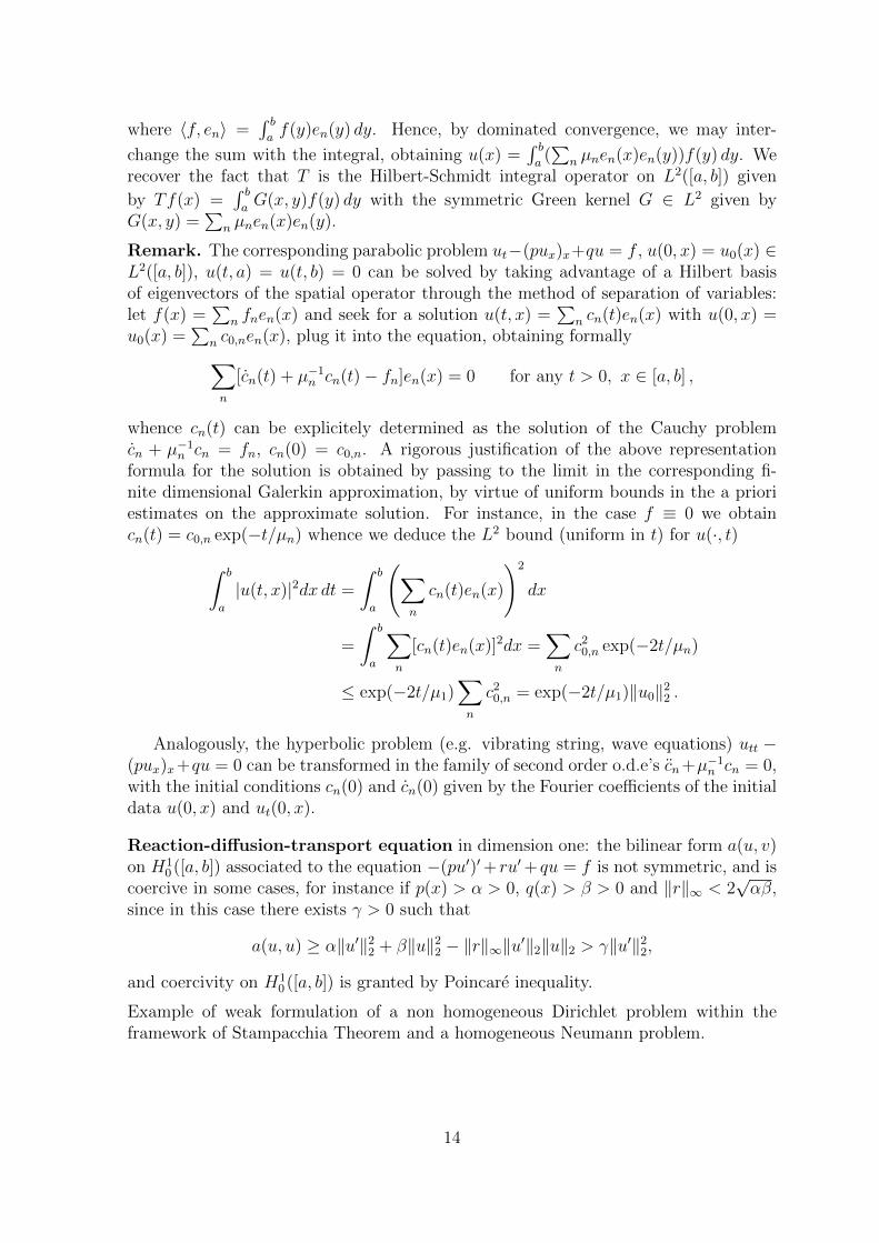
Remark. The corresponding parabolic problem ut−(pux)x+qu = f , u(0, x) = u0(x) ∈L2([a, b]), u(t, a) = u(t, b) = 0 can be solved by taking advantage of a Hilbert basisof eigenvectors of the spatial operator through the method of separation of variables:let f(x) =

∑n fnen(x) and seek for a solution u(t, x) =

∑n cn(t)en(x) with u(0, x) =

u0(x) =∑

n c0,nen(x), plug it into the equation, obtaining formally∑n

[cn(t) + µ−1n cn(t)− fn]en(x) = 0 for any t > 0, x ∈ [a, b] ,

whence cn(t) can be explicitely determined as the solution of the Cauchy problemcn + µ−1

n cn = fn, cn(0) = c0,n. A rigorous justification of the above representationformula for the solution is obtained by passing to the limit in the corresponding fi-nite dimensional Galerkin approximation, by virtue of uniform bounds in the a prioriestimates on the approximate solution. For instance, in the case f ≡ 0 we obtaincn(t) = c0,n exp(−t/µn) whence we deduce the L2 bound (uniform in t) for u(·, t)∫ b

a

|u(t, x)|2dx dt =

∫ b

a

(∑n

cn(t)en(x)

)2

dx

=

∫ b

a

∑n

[cn(t)en(x)]2dx =∑n

c20,n exp(−2t/µn)

≤ exp(−2t/µ1)∑n

c20,n = exp(−2t/µ1)‖u0‖2

2 .

Analogously, the hyperbolic problem (e.g. vibrating string, wave equations) utt −(pux)x+qu = 0 can be transformed in the family of second order o.d.e’s cn+µ−1

n cn = 0,with the initial conditions cn(0) and cn(0) given by the Fourier coefficients of the initialdata u(0, x) and ut(0, x).

Reaction-diffusion-transport equation in dimension one: the bilinear form a(u, v)on H1

0 ([a, b]) associated to the equation −(pu′)′+ ru′+ qu = f is not symmetric, and iscoercive in some cases, for instance if p(x) > α > 0, q(x) > β > 0 and ‖r‖∞ < 2

√αβ,

since in this case there exists γ > 0 such that

a(u, u) ≥ α‖u′‖22 + β‖u‖2

2 − ‖r‖∞‖u′‖2‖u‖2 > γ‖u′‖22,

and coercivity on H10 ([a, b]) is granted by Poincare inequality.

Example of weak formulation of a non homogeneous Dirichlet problem within theframework of Stampacchia Theorem and a homogeneous Neumann problem.

14

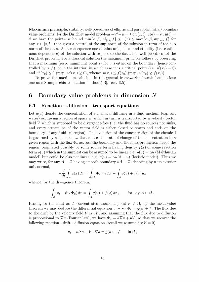
Maximum principle, stability, well-posedness of elliptic and parabolic initial/boundaryvalue problems: for the Dirichlet model problem −u′′+u = f on [a, b], u(a) = α, u(b) =β we have the pointwise bound minα, β, inf [a,b] f ≤ u(x) ≤ maxα, β, sup[a,b] f forany x ∈ [a, b], that gives a control of the sup norm of the solution in term of the supnorm of the data. As a consequence one obtains uniqueness and stability (i.e. contin-uous dependence) of the solution with respect to the data, i.e. well-posedness of theDirichlet problem. For a classical solution the maximum principle follows by observingthat a maximum (resp. minimum) point x0 for u is either on the boundary (hence con-trolled by α, β), or in the interior, in which case it is a critical point (i.e. u′(x0) = 0)and u′′(x0) ≤ 0 (resp. u′′(x0) ≥ 0), whence u(x0) ≤ f(x0) (resp. u(x0) ≥ f(x0)).

To prove the maximum principle in the general framework of weak formulationsone uses Stampacchia truncation method ([B], sect. 8.5).

6 Boundary value problems in dimension N

6.1 Reaction - diffusion - transport equations

Let u(x) denote the concentration of a chemical diffusing in a fluid medium (e.g. air,water) occupying a region of space Ω, which in turn is transported by a velocity vectorfield V which is supposed to be divergence-free (i.e. the fluid has no sources nor sinks,and every streamline of the vector field is either closed or starts and ends on theboundary of any fluid subregion). The evolution of the concentration of the chemicalis governed by a balance law that relates the rate of change of the concentration in agiven region with the flux Φu accross the boundary and the mass production inside theregion, originated possibly by some source term having density f(x) or some reactionterm g(u) which in the simplest can be assumed to be linear, i.e. g(u) = αu (Malthusianmodel) but could be also nonlinear, e.g. g(u) = αu(β − u) (logistic model). Thus wemay write, for any A ⊂ Ω having smooth boundary ∂A ⊂ Ω, denoting by n its exteriorunit normal,

− d

dt

∫A

u(x) dx =

∫∂A

Φu · n dσ +

∫A

g(u) + f(x) dx

whence, by the divergence theorem,∫A

(ut − div Φu) dx =

∫A

g(u) + f(x) dx , for any A ⊂ Ω .

Passing to the limit as A concentrates around a point x ∈ Ω, by the mean-valuetheorem we may deduce the differential equation ut−∇ ·Φu = g(u) + f . The flux dueto the drift by the velocity field V is uV , and assuming that the flux due to diffusionis proportional to ∇u (Fourier law), we have Φu = k∇u + uV , so that we recover thefollowing reaction - drift - diffusion equation (recall we assume divV = 0)

ut − k∆u+ V · ∇u = g(u) + f in Ω ,

15

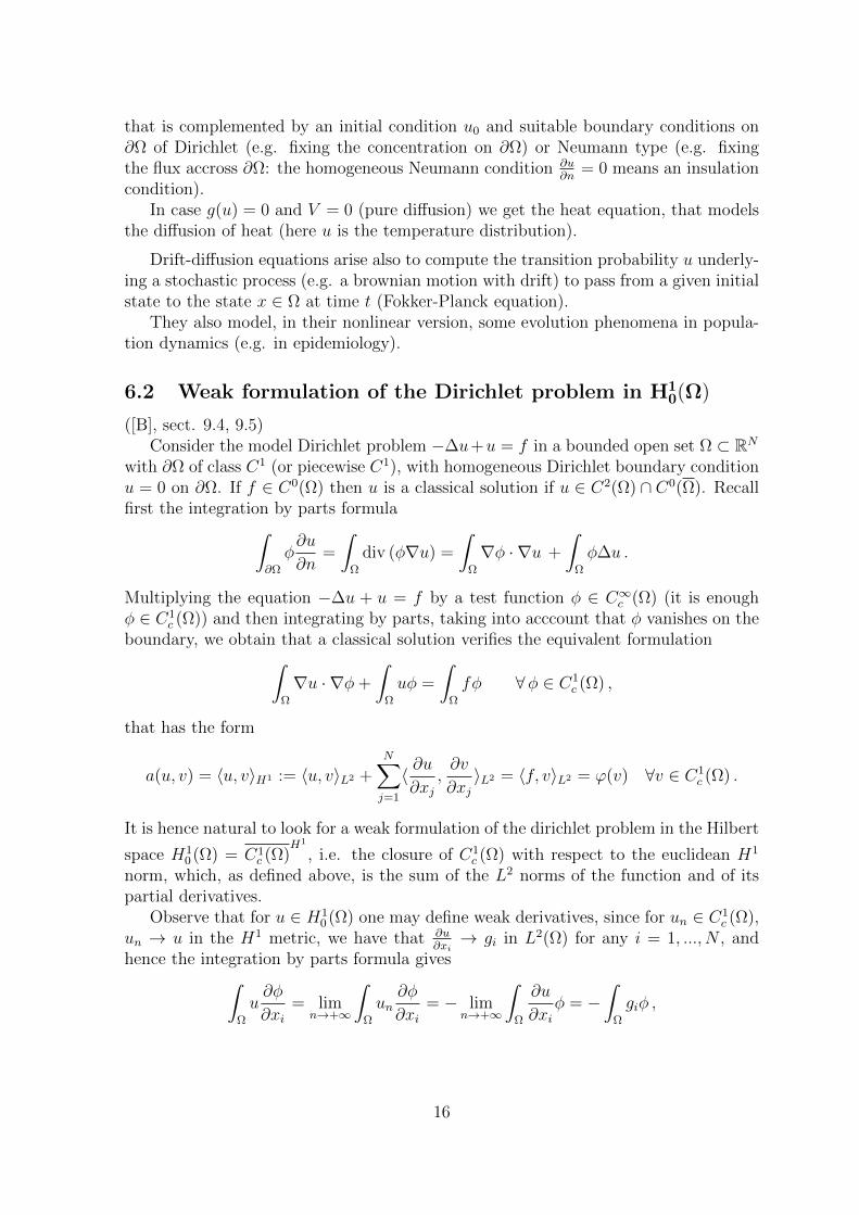
that is complemented by an initial condition u0 and suitable boundary conditions on∂Ω of Dirichlet (e.g. fixing the concentration on ∂Ω) or Neumann type (e.g. fixingthe flux accross ∂Ω: the homogeneous Neumann condition ∂u

∂n= 0 means an insulation

condition).In case g(u) = 0 and V = 0 (pure diffusion) we get the heat equation, that models

the diffusion of heat (here u is the temperature distribution).

Drift-diffusion equations arise also to compute the transition probability u underly-ing a stochastic process (e.g. a brownian motion with drift) to pass from a given initialstate to the state x ∈ Ω at time t (Fokker-Planck equation).

They also model, in their nonlinear version, some evolution phenomena in popula-tion dynamics (e.g. in epidemiology).

6.2 Weak formulation of the Dirichlet problem in H10(Ω)

([B], sect. 9.4, 9.5)Consider the model Dirichlet problem −∆u+u = f in a bounded open set Ω ⊂ RN

with ∂Ω of class C1 (or piecewise C1), with homogeneous Dirichlet boundary conditionu = 0 on ∂Ω. If f ∈ C0(Ω) then u is a classical solution if u ∈ C2(Ω) ∩ C0(Ω). Recallfirst the integration by parts formula∫

∂Ω

φ∂u

∂n=

∫Ω

div (φ∇u) =

∫Ω

∇φ · ∇u +

∫Ω

φ∆u .

Multiplying the equation −∆u + u = f by a test function φ ∈ C∞c (Ω) (it is enoughφ ∈ C1

c (Ω)) and then integrating by parts, taking into acccount that φ vanishes on theboundary, we obtain that a classical solution verifies the equivalent formulation∫

Ω

∇u · ∇φ+

∫Ω

uφ =

∫Ω

fφ ∀φ ∈ C1c (Ω) ,

that has the form

a(u, v) = 〈u, v〉H1 := 〈u, v〉L2 +N∑j=1

〈 ∂u∂xj

,∂v

∂xj〉L2 = 〈f, v〉L2 = ϕ(v) ∀v ∈ C1

c (Ω) .

It is hence natural to look for a weak formulation of the dirichlet problem in the Hilbert

space H10 (Ω) = C1

c (Ω)H1

, i.e. the closure of C1c (Ω) with respect to the euclidean H1

norm, which, as defined above, is the sum of the L2 norms of the function and of itspartial derivatives.

Observe that for u ∈ H10 (Ω) one may define weak derivatives, since for un ∈ C1

c (Ω),un → u in the H1 metric, we have that ∂u

∂xi→ gi in L2(Ω) for any i = 1, ..., N , and

hence the integration by parts formula gives∫Ω

u∂φ

∂xi= lim

n→+∞

∫Ω

un∂φ

∂xi= − lim

n→+∞

∫Ω

∂u

∂xiφ = −

∫Ω

giφ ,

16

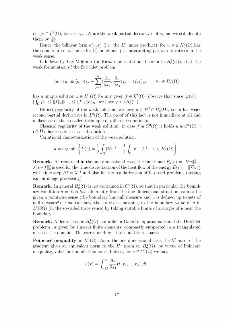
i.e. gi ∈ L2(Ω), for i = 1, ..., N are the weak partial derivatives of u, and we still denotethem by ∂u

∂xi.

Hence, the bilinear form a(u, v) (i.e. the H1 inner product), for u, v ∈ H10 (Ω) has

the same representation as for C1c functions, just interpreting partial derivatives in the

weak sense.It follows by Lax-Milgram (or Riesz representation theorem in H1

0 (Ω)), that theweak formulation of the Dirichlet problem

〈u, v〉H1 ≡ 〈u, v〉L2 +N∑j=1

〈 ∂u∂xj

,∂v

∂xj〉L2 = 〈f, v〉L2 ∀v ∈ H1

0 (Ω)

has a unique solution u ∈ H10 (Ω) for any given f ∈ L2(Ω) (observe that since |ϕ(v)| =

|∫

Ωfv| ≤ ‖f‖2‖v‖2 ≤ ‖f‖2‖v‖H1 we have ϕ ∈ (H1

0 )′ ).

Hilbert regularity of the weak solution: we have u ∈ H2 ∩H10 (Ω), i.e. u has weak

second partial derivatives in L2(Ω). The proof of this fact is not immediate at all andmakes use of the so-called technique of difference quotients.

Classical regularity of the weak solution: in case f ∈ C0(Ω) it holds u ∈ C2(Ω) ∩C0(Ω), hence u is a classical solution.

Variational characterization of the weak solution:

u = arg min

F (v) =

1

2

∫Ω

|∇v|2 +1

2

∫Ω

|v − f |2 , v ∈ H10 (Ω)

.

Remark. As remarked in the one dimensional case, the functional Fλ(v) = ‖∇u‖22 +

λ‖v−f‖22 is used for the time discretization of the heat flow of the energy E(v) = ‖∇u‖2

2

with time step ∆t = λ−1 and also for the regularization of ill-posed problems (arisinge.g. in image processing).

Remark. In general H10 (Ω) is not contained in C0(Ω), so that in particular the bound-

ary condition u = 0 on ∂Ω, differently from the one dimensional situation, cannot begiven a pointwise sense (the boundary has null measure and u is defined up to sets ofnull measure!). One can nevertheless give a meaning to the boundary value of u inL2(∂Ω) (in the so-called trace sense) by taking suitable limits of averages of u near theboundary.

Remark. A dense class in H10 (Ω), suitable for Galerkin approximation of the Dirichlet

problems, is given by (linear) finite elements, compactly supported in a triangulatedmesh of the domain. The corresponding stiffnes matrix is sparse.

Poincare inequality on H10 (Ω). As in the one dimensional case, the L2 norm of the

gradient gives an equivalent norm to the H1 norm on H10 (Ω), by virtue of Poincare

inequality, valid for bounded domains. Indeed, for u ∈ C1c (Ω) we have

u(x) =

∫ x1

−M

∂u

∂x1

(t, x2, ..., xN) dt ,

17

where Ω ⊂ BM(0). By Cauchy-Schwarz we obtain |u(x)|2 ≤ 2M∫MM|∂1u|2 dt, and

integrating on Ω we obtain, by Fubini,∫Ω

|u(x)|2 dx ≤ 4M2

∫Ω

∣∣∣∣ ∂u∂x1

∣∣∣∣2 dx ≤ 4M2

∫Ω

|∇u(x)|2 dx ,

i.e. ‖u‖L2(Ω) ≤ 2M‖∇u‖L2(Ω).

6.3 Elliptic problems in divergence form

([B], Theorem 9.23)For aij(x) ∈ L∞(Ω), i, j = 1, ..., N , ai(x) ∈ L∞(Ω) for i = 0, ..., N , f(x) ∈ L2(Ω)

consider the weak formulation in H10 (Ω) of the following problem in divergence form

(anisotropic diffusion - transport - reaction equation)

−N∑

i,j=1

∂

∂xi

(aij(x)

∂u

∂xj

)+

N∑i=1

ai(x)∂u

∂xi+ a0(x)u = f(x) in Ω

with u = 0 on ∂Ω. The weak formulation reads∫Ω

N∑i,j=1

aij(x)∂u

∂xj

∂v

∂xi+

N∑i=1

ai(x)∂u

∂xiv + a0(x)uv =

∫Ω

fv ∀ v ∈ H10 (Ω) ,

Hence it is of the form a(u, v) = ϕ(v) (with a non symmetric). If∑N

i,j=1 aij(x)ξiξj ≥α|ξ|2 for some α > 0 then, for some sufficiently large λ > 0 the bilinear form a(u, v) +λ〈u, v〉L2 is coercive on H1

0 (Ω) (compare the argument in the one dimensional case),hence by Lax-Milgram, for any Φ ∈ H1

0 (Ω)′ there exists a unique solution of a(u, v) +λ〈u, v〉L2 = ϕ(v) for any v ∈ H1

0 (Ω).Denoting by f 7→ Tf the solution operator, we have T : L2(Ω)→ H1

0 (Ω) ⊂ L2(Ω),with compact embedding (cfr. Rellich theorem), hence T ∈ K(L2(Ω)) and u solvesthe fixed point equation u = T (f + λu). Setting w = f + λu we have that w solvesw = λTw + f , i.e. (I − λT )w = f . Suppose f = 0 (hence w = λu). Then, either thehomogeneous equation u = λTu is uniquely solvable (if and only if the original equationhas zero as unique solution, and this is precisely the case for instance if a0(x) ≥ β > 0,by the maximum principle (see [B], Remark 27 after Theorem 9.27), and hence thereexists a unique solution u ∈ H1

0 (Ω) for any f ∈ L2(Ω), or the homogeneous equationhas a (finite) d-dimensional set of solutions, whence the original problem is solvable iff is orthogonal to a suitable d-dimensional subspace of L2(Ω).

18

7 Distributions, Sobolev spaces and functions of

bounded variation

7.1 Distributions and distributional derivatives

Given u ∈ L1loc(Ω), we may identify u with the distribution (linear functional on C∞c (Ω))

Tu(φ) =∫

Ωu(x)φ(x) dx. One advantage of the distributional point of view is to embed

functions in dual spaces, where the Banach-Alaoglu compactness theorem holds true.

Recall Banach-Alaoglu theorem: given a Banach space X, bounded sequences in X ′

are relatively compact with respect to the weak* topology, i.e. for Tj ∈ X ′, ‖Tj‖∗ ≤ C,there exists T ∈ X ′ such that, up to a subsequence, Tj(φ) → T (φ) for any φ ∈ X.Remark that the weak* topology is a priori weaker than the weak topology, where onetests convergence against any element of the dual space, i.e. in this case (X ′)′ = X ′′,which contains strictly X in the non reflexive case. Of course, if X is reflexive, weakand weak* convergence do coincide.

Supposing for simplicity that Ω is bounded and u ∈ L1(Ω), we have |Tu(φ)| ≤‖u‖1‖φ‖∞. i.e. Tu extends to a bounded functional on C0

c (Ω) = C∞c (Ω)L∞

, the spaceof continuous functions vanishing on ∂Ω. Moreover,

‖Tu‖∗ = supTu(φ), ‖φ‖∞ ≤ 1 = ‖u‖1

as it follows by considering test functions φ converging to the function 1u>0−1u<0,which in turn gives that uφ converges to |u| = u+ + u−. We thus have an isometricinjection L1(Ω)→ [C0

c (Ω)]∗.

Measures as distributions. The distribution Tµ associated to a (possibly σ-finite)Radon measure µ on Ω is defined in the same way: Tµ(φ) ≡ 〈Tµ, φ〉 =

∫Ωφ(x)dµ(x). For

any µ ∈M(Ω) (the space of finite Radon measures on Ω) it actually holds Tµ ∈ [C0c (Ω)]∗

and‖Tµ‖∗ = sup〈Tµ, φ〉 , φ ∈ C0

c (Ω) , ‖φ‖∞ ≤ 1 = |µ|(Ω),

where |µ| = µ++µ− is the total variation measure of µ = µ+−µ− (Hahn decomposition)and ‖µ‖ = |µ|(Ω) is the total variation of the measure µ on Ω (as for L1 function, onetests with a function φ ' 1sptµ+ − 1sptµ−).

For µ, ν ∈ M(Ω) two Radon measures on Ω, Tµ = Tν implies∫

Ωφ(x) dµ(x) =∫

Ωφ(x) dν(x), for any φ ∈ C∞c (Ω), so that by considering φj converging to the char-

acteristic function of an open subset A ⊂ Ω se obtain, by the dominated convergencetheorem, that µ(A) = ν(A) for any A ⊂ Ω open, hence µ = ν by the regularity ofRadon measures. Hence µ 7→ Tµ gives an injection M(Ω) → [C0

c (Ω)]∗. Hence (finiteand σ-finite) Radon measures in Ω are distributions (of order zero).

Example (Dirac mass as a distribution): let δ0 be the Dirac mass concentratedat 0 ∈ RN . We have

Tδ0(φ) =

∫RNφdδ0 = φ(0) ,

19

since∫RNφdδ0 = supc0 ∈ R, φ(x) ≥

∑ci1Ei(x), E0 3 0 = supc0 ≤ φ(0) = φ(0) .

in particular

‖Tδ0‖∗ = supφ(0), φ ∈ C0c (RN), ‖φ‖∞ ≤ 1 = 1.

Recall Riesz representation theorem: µ ∈ M(Ω) 7→ Tµ ∈ [C0c (Ω)]∗ is an isomor-

phism of Banach spaces, where the norm of a measure µ ∈ M(Ω) is given by itstotal variation ‖µ‖ = |µ|(Ω). In particular, it holds |µ|(Ω) = ‖µ‖ = ‖Tµ‖∗. Weak*compactness and convergence in the sense of measures: by the Banach-Alaoglu theo-rem (bounded sets in the dual of a Banach space are relatively compact with respectto the weak* topology), a sequence of equibounded Radon measures µn on Ω (i.e.|µn|(Ω) ≤ C) is weakly* compact, i.e. there exists a subsequence µnk and a measure

µ such that µnk∗ µ in M(Ω), or in other words

∫Ωφ(x) dµnk(x) →

∫Ωφ(x) dµ(x) for

any φ ∈ C0c (Ω).

The space of Radon measures is suited to solve optimization problems involving L1 ortotal variation norms. For example, for Y ⊂ M(Ω) , Y closed convex and bounded,consider the minimization problem

inf‖µ‖ = µ(Ω) = ‖Tµ‖∗, µ ∈ Y .

Then, since Y is closed and convex it is weakly* closed by Hahn-Banach, and since itis also bounded it is weakly* compact by Banach-Alaoglu. The total variation normis weakly* lowersemicontinuous being characterized as a supremum, as a dual norm.Hence the existence of a minimizer in Y is guaranteed by Weierstrass theorem (orequivalently by the direct method of the calculus of variations).

Example: the Monge-Kantorovich optimal mass transport problem consistsin minimizing the transportation cost of displacing a given amount M of mass (oreconomical goods) whose initial distribution in a (metric measure) space X is describedby a measure µ1 of total mass µ1(X) = M , in order to reach a final destinationdescribed by a measure µ2 in a (metric measure) space Y (with total mass µ2(Y ) = M).Observe that, for M = 1, µ1 and µ2 are probability measures. Denote by c(x, y) thetransportation cost function for displacing a unit of mass (or good) from location x ∈ Xto location y ∈ Y (if X and Y are subset of a euclidean space, say RN , typical costfunctions are c(x, y) = |x− y| or c(x, y) = |x− y|2), and denote by T ⊂M(X×Y ) theset of transport plans from µ1 to µ2, i.e. the measures µ on X × Y having marginalsµ1 and µ2 (i.e.

∫Ydµ(x, y) = µ1(x) and

∫Xdµ(x, y) = µ2(y)). Observe that in case µ1

and µ2 are discrete probability measures this is a linear programming problem. Theset T is an affine (hence convex) closed subset of M(X × Y ) (fixing the marginals

20

is a continuous constraint with respect to the convergence of measures), hence theconstrained optimization problem

minµ∈T

F (µ) =

∫X×Y

c(x, y)dµ(x, y) .

admit a solution by Banach-Alaoglu theorem, assuming lower semi-continuity forthe cost function.

Derivative of a distribution: for u and Tu as above, we can define the (i-th partial)derivative of Tu as the linear functional ∂iTu(φ) = −

∫Ωu ∂φ∂xi

. A priori, since |∂iTu(φ)| ≤‖u‖1‖∂iφ‖∞, we have ∂iTu ∈ [C1

c (Ω)]∗. This definition is coherent with the integrationby parts formula, since for smooth functions u one has ∂iTu(φ) = T∂iu(φ) for any testfunction φ. In particular, since integration by parts holds true for functions in W 1,p(Ω),we have that Sobolev functions may be defined as those functions in Lp(Ω) such thattheir distributional derivatives are (associated to) functions in Lp(Ω).

Example: for u(x) = |x|, x ∈ R, we have

−∫Ruφ′ = −

∫ 0

−∞xφ′(x) dx+

∫ +∞

0

xφ′(x) dx = −∫ 0

−∞φ(x) dx+

∫ +∞

0

φ(x) dx ,

hence it follows that (Tu)′ = Tv where v(x) = 1 if x > 0 and v(x) = −1 if x < 0.

Example (distributional derivative of the Heaviside function): consider theHeaviside function H on R, i.e H(x) = 1 for x ≥ 0, and H(x) = 0 for x < 0, andconsider the following approximating sequence for H, given by uj(x) = 1 if x ≥ j−1

and uj(x) = j · x for 0 ≤ x ≤ j−1, uj(x) = 0 for x < 0. We have (Tuj)′ = −Tvj

where vj(x) = j for 0 ≤ x ≤ j−1, and vj(x) = 0 elsewhere in R. Notice that ‖Tvj‖∗ =∫R vj(x) dx = 1 for any j ∈ N, hence, up to a subsequence, Tvj T weakly* in [C0

c (R)]∗

by Banach-Alaloglu theorem, i.e.

T (φ) = limjTvj(φ) = j

∫ 1/j

0

φ(x) dx = φ(0) = Tδ0(φ) ∀φ ∈ C0c (R) .

On the other hand, we have −T (φ) = limj Tuj(φ′) = TH(φ′), hence T = (TH)′. Hence,

in R we have Tδ0 = (TH)′, i.e. the Dirac mass is the distributional derivative of theHeaviside function. Observe that the Heaviside function has a classical derivativea.e. (actually everywhere except in the origin), which is identically zero, while thedistributional derivative of H keeps the information on the unit jump of H at theorigin.

7.2 The Sobolev spaces W1,p(Ω)

([B], sect. 9.1) Sobolev spaces arise naturally when solving PDE’s through weak for-mulations, or in order to deal with optimization problems, such as for example the

21

variational (minimum) problem

min

F (v) =

∫Ω

|∇v|p + λ

∫Ω

|v − f |q, v = 0 on ∂Ω

that arises in many contexts, especially in the cases q = 2 (least square) and p = 1, 2, orin the case 1 < p = q. Existence of minimizers is found in suitable Hilbert and Banachspaces called Sobolev spaces or Functions of Bounded Variation, where the dual spacetype norms are controlled by F , ensuring at a glance lowersemicontinuity of F andcompactness of minimizing sequences with respect to weak (or weak*) convergences.

We refer to [B], sect. 9.1 for details. Definition of W 1,p(Ω) as the space of Lp

functions having weak partial derivatives in Lp(Ω). The W 1,p norm. Some elementaryproperties of W 1,p(Ω): completeness, reflexivity, separability, according to the exponentp. The Hilbert space H1(Ω) = W 1,2(Ω). The space W 1,∞(Ω) coincides with the spaceof Lipschitz functions on Ω, when Ω is a regular domain (with boundary of class C1 orlipschitz).

In case Ω = RN Sobolev norms may be defined through suitable weighted norms onL2(RN

ω ), where ω is the frequency (or Fourier) variable. For example, by Planchereltheorem, we have ‖u‖2

H1 =∫RN (1 + 4π|ω|2)|u(ω)|2dω.

The closed subspace W 1,p0 (Ω) ⊂ W 1,p(Ω) is defined as the closure with respect of

the W 1,p norm of C1c (Ω), and is suited to deal with homogeneous Dirichlet boundary

conditions. On W 1,p0 (Ω) there holds the Poincare inequality ‖v‖p ≤ C‖∇v‖p.

Density of smooth functions in W 1,p(Ω): one extends a function u ∈ W 1,p(Ω) by zerooutside Ω, obtaining a function u, and then regularize u by convolution with a familyof smoothing kernels (or symmetric mollifiers) ρn ∈ C∞c (RN) such that ρn = nNρ1(nx),ρ1 ≥ 0 supported in the unit ball and

∫B1ρ1 = 1. Denoting by un = u ∗ ρn, we have

un ∈ C∞c (RN), and one deduces un|Ω → u in Lp(Ω), while due to the discontinuityof u on the boundary of Ω, we deduce ∇un|ω → ∇u in [Lp(ω)]N for any ω ⊂⊂ Ω. Ifthe boudary is regular, say piecewise C1 then one may prove by slightly modifying theconstruction of un that actually there exists un ∈ C∞c (RN) such that ∇un|Ω → ∇u in[Lp(Ω)]N .

Recall the notion of approximation of identity: for ρn as above, consider the (positive)measures µn = ρn(x) dx. We have µn δ0 in the sense of measures, where δ0 is theDirac mass concentrated at zero. Indeed, since the support of ρn is B1/n and the totalintegral is 1, we have µn(A) → 0 = δ0(A) if the open set A does not contain 0, andµn(A)→ 1 = δ0(A) otherwise. One concludes by using the regularity of both (Radon)measures: if they coincide on open sets, they coincide on any Borel set.

Recall further that ρn dx δ0 implies ρn ∗ u → u in Lp(RN) and ‖ρn ∗ u‖p ≤‖ρn‖1‖u‖p = ‖u‖p. Similarly, ∂i(ρn ∗ u) → ∂iu in Lp(RN) for any ∈ W 1,p(RN) ≡W 1,p

0 (RN).

Characterization of maps in W 1,p(Ω), Ω ⊂ RN bounded, for p > 1 (see [B], Proposition9.3 for a clean statement):

22

1) Lp functions whose (weak) derivatives are identified (in the distributional sense) tobounded linear functionals on Lp

′(Ω),

2) Lp functions having uniformly bounded differential quotients w.r.t the Lp norm.

(for the notion of distribution and distributional derivative see next section).

In case p = 1 the property corresponding to 1) is expressed by

1’) L1 functions whose distributional derivatives are identified to bounded linear func-tionals on C0

c (Ω).

In case p = 1 properties 1’) and 2) are still equivalent, and they characterize thespace BV (Ω) ⊂ L1(Ω) of functions of bounded variation, which is strictly larger thanW 1,1(Ω).

Some comments on properties 1) (resp. 1’) ) and 2). Property 1) emphasize the factthat the weak derivative, seen a distribution, belongs to a dual space, yielding byBanach-Alaoglu weak (resp. weak*) compactness for sequences of gradients uniformlybounded with respect to the dual norm, which by the Riesz representation theoremcorresponds, in case p > 1, to the Lp norm, while in case p = 1, to the so-called totalvariation norm, which is the norm on the space of Radon measures on Ω, M(Ω) ≡[C0

c (Ω)]∗ by Riesz representation theorem.

Remark. (Variational problems in W1,p) Minimizing sequences for the functionalF (v) = ‖∇v‖pp + ‖v − f‖pp are uniformly bounded with respect to the W 1,p norm,hence they converge weakly (up to a subsequence) in W 1,p for p > 1. Hence, by lowersemicontinuity of F with respect to weak convergence (Lp norms, being equivalent tothe dual norm in (Lp

′)′ are lower semicontinuous by Banach - Steinhaus) we obtain

existence of minimizers of F in W 1,p.

In the case p = 1 there exist sequences uniformly bounded with respect to the W 1,1

norm that do not converge in W 1,1 (for example functions approximating the Heavisidefunction, see the example in the previous section), so that in particular W 1,1 is nota suitable ambient space for variational problems. On the other hand, property 1’)ensures weak* compactness in [C0

c (Ω)]∗ of sequence of gradients uniformly bounded inL1, so that in particular they converge in BV (Ω) (see section 7.3), which is thereforesuited to handle variational problems for functionals involving the L1 norm of thegradient, such as the so-called Rudin - Osher - Fatemi model for image processingFλ(v) = ‖∇v‖1 + λ‖v − f‖2

2.

Property 2) implies that the hypothesis of Frechet-Kolmogorov theorem (which givesa criterion for compactness in the strong topology of Lp(Ω) for p ≥ 1) is satisfied. Inparticular, the injection W 1,p(Ω) → Lp(Ω) for p > 1 (resp. the injection BV (Ω) →L1(Ω)) is compact (Rellich-Kondrachov compact embedding theorem).

Proof of the compact injection of W 1,p(Ω) in Lp(Ω) for bounded Ω ⊂ RN : if F is abounded family of W 1,p(Ω), and ω ⊂⊂ Ω, then ρn ∗ F|ω is ε-close to F|ω for large n,and uniformly bounded in L∞ and equi-uniformly continuous, hence relatively compact

23

with respect to the ‖ · ‖∞ norm by Ascoli-Arzela, so that in particular it is relativelycompact in Lp(ω). An ε-net for ρn ∗ F|ω in Lp(ω) is then a 2ε-net for F|ω and a 3ε-netfor F in Lp(Ω) if ω is sufficiently close in measure to Ω.

7.3 BV functions and variational problems

([G])Distributional gradient of a function u ∈ L1(Ω): it is a vector distribution defined by

〈DTu, ~ϕ〉 = −〈Tu, div ~ϕ〉 for ~ϕ ∈ [C∞c (Ω)]N . Remark that for distributions associatedto functions u of class C1 previous formula coincides with Gauss-Green (or integrationby parts) formula.

Definition of the space BV (Ω) (functions of bounded variation): u ∈ BV (Ω) if u ∈L1(Ω) and the distributional gradient Du = (∂1u, ..., ∂Nu) is a (vector) Radon measure~µ = (µ1, ..., µN), which satisfies the integration by part formula (Gauss-Green)∫

Ω

u div ~φ = −∫

Ω

~φ · d~µ for any ~φ ∈ [C0c (Ω)]N .

In other words, u ∈ BV (Ω) if u ∈ L1(Ω) and ∂iTu(ϕ) =∫

Ωϕdµi = Tµi(φ).

Total variation of a vector Radon measure: for ~µ = (µ1, ..., µn) with µi ∈M(Ω) =(C0

c (Ω))′ we have the decomposition ~µ = ~ν|~µ|, where |~µ| is a positive measure (calledthe total variation measure) and |~ν(x)| = 1 for |~µ| a.e. x ∈ Ω. The total variation of~µ is defined as the dual norm in [C0

c (Ω)]∗

‖~µ‖∗ = sup

∫Ω

~φ · d~µ =

∫Ω

~φ · ~ν d|~µ| , ~φ ∈ [C0c (Ω)]n, ‖~φ‖∞ ≤ 1

= |~µ|(Ω).

For u ∈ BV (Ω) we define its BV norm

‖u‖BV (Ω) = ‖u‖L1(Ω) + |Du|(Ω) .

Remark that for u ∈ W 1,1(Ω) the BV norm coincides with the W 1,1 norm. Endowedwith such a norm, BV (Ω) is a Banach space.

Characterization of BV (Ω): properties 1’) and 2) in previous section are equivalentcharacterizations of BV (Ω). In particular, 2) implies compactness in the strong L1

topology of sequences of functions equibounded with respect to the BV norm.

Example: the characteristic function 1E of an open bounded set E ⊂ Rn with ∂E∩Ωof class C1 belongs to BV (Ω), since by Gauss-Green formula

D1E(~φ) = −∫E

div ~φ dx = −∫∂E

~φ · ~n dσ ,

where ~n is the unit outer normal to ∂E and dσ is the surface measure on ∂E, sothat |D1E(~φ)| ≤ ‖~φ‖∞ · Area(∂E ∩ Ω), i.e. D1E is a vector Radon measure, and in

24

particular D1E = ~ν|D1E|, where ~ν(x) = −~n(x) is the inner unit normal to ∂E∩Ω and

|D1E| = dσ. By a suitable choice of the test function ~φ in such a way that |~φ(x)| ≤ 1

and ~φ = −~n on ∂E ∩ Ω one gets |D1E|(Ω) = Area(∂E ∩ Ω).

An example of variational problem in BV : the Rudin-Osher-Fatemi modelF (u) = |Du|(Ω) + 1

2‖u − f‖2

L2(Ω), for u ∈ BV (Ω) is suitable in image processing (u

denotes for instance the grey level of an image), since it has the ability to regularize(denoise) a given image f (identified as its grey level function) by preserving at thesame time edges and boundaries, since characteristic functions are members of BV .Existence of a minimizer in BV (Ω) on a bounded Ω is guaranteed because F controlsthe full BV norm and F is lower semicontinuous with respect to the weak* convergenceof the total variation and weak L2 convergence. Its Euler-Lagrange equation results ina nonlinear PDE.

An example of geometric variational problem: the isoperimetric and the iso-volumetric problem within the class of finite perimeter sets. The two problem areequivalent (and dual each other), since they amount to maximize the (dilation invari-

ant) isoperimetric ratio |Ω|n−1n /|∂Ω|.

Definition of finite perimeter (or Caccioppoli) sets in Ω ⊂ Rn: they are Lebesguemeasurable sets E ⊂ Rn such that

PΩ(E) ≡ |D1E|(Ω) ≡ sup

∫E∩Ω

div~φ , ‖~φ‖∞ ≤ 1, ~φ ∈ [C∞c (Ω)]n< +∞,

in other words 1E ∈ BV (Ω).Observe that for finite perimeter sets E ⊂ Rn, the Sobolev embedding theorem

BV (Rn)→ Lnn−1 (Rn) applied to 1E yields the isoperimetric inequality

|E|n−1n ≤ C|D1E|(Rn) = CPRn(E).

The minimal constant C > 0 in the above inequality corresponds to the isoperimetricratio of a round ball in Rn.

Weak formulation of the isovolumetric problem in the class of finite perimeter setsin Rn: fix R > 1 (sufficiently large) and set

P =

E ⊂ BR(0), Ln(E) =

∫Rn

1E dLn = 1, 1E ∈ BV (Rn)

,

i.e. P contains sets E ⊂ BR(0) having unit volume and finite perimeter ‖D1E‖ ≡|D1E|(Rn). Consider the isovolumetric problem

minE∈P‖D1E‖ .

If En ∈ P is a minimizing sequence, i.e. ‖D1En‖ → infF∈P ‖D1F‖, we have

‖1En‖BV = 1 + ‖D1En‖ ≤ C,

25

so that, up to a subsequence, 1En → 1E in L1(B2R(0)) since the supports of En arecontained in B2R(0) and hence there holds the compact embedding of BV (B2R(0))in L1(B2R(0)) . We immediately deduce E ⊂ BR(0) and Ln(E) = 1. Moreover, we

have D1En(~φ) → D1E(~φ) for any ~φ ∈ [C∞c (Rn)]n (i.e. convergence in the sense ofdistributions) and

‖∇1E‖ ≤ lim infn→+∞

‖∇1En‖ = infF∈P‖∇1F‖

by lower semicontinuity of the total variation norm. Hence E has minimum perimeterin the class P .

The regularity theory (based for example on Steiner symmetrization) allows toconclude that the optimal set E is the unit volume round ball in Rn.

26