BeBeC-2014-01

1

FUNCTIONAL BEAMFORMING

Robert P. Dougherty1

1OptiNav, Inc.

1414 127th

PL NE #106, 98004, Bellevue, WA, USA

ABSTRACT

A new beamforming algorithm is introduced. It is called Functional Beamforming

because it uses the mathematics of functions of matrices. The algorithm depends on an

exponent parameter. The array Cross Spectral Matrix is raised to the power of the

reciprocal of this exponent in the functional sense. Conventional Frequency Domain

Beamforming is applied using the modified CSM, and the values of the resulting

beamform map are raised to power of the non-reciprocal exponent. For large values of the

exponent, array sidelobes are essentially eliminated. This increases flexibility in array

design and dramatically increases the dynamic range of the system so that new sources

may be discovered. Theory is given that proves that the method will not eliminate or even

reduce true sources if the steering vector is accurate. This depends on the quality the array

calibration, but the requirements are not extraordinary. Examples are given comparing the

method with Robust Adaptive Beamforming, CLEAN-SC, Orthogonal Beamforming, and

to some degree, Linear Programming. A previously unknown noise source of Boeing 747

desk models is shown.

1 INTRODUCTION

For many years, beamforming in acoustics and other fields has made use of sparse arrays in

order to obtain acceptable results over a wide frequency range with a constrained number of

sensors. Conventional beamforming (Frequency Domain Beamforming, FDBF) produces

image maps with high sidelobe levels and severely limited dynamic range. Deconvolution

methods have been applied to post process the complete maps [1,2] or decompose the cross

spectral matrix into parts due to individual sources [3-5]. These methods can increase the

dynamic range to some degree, but also can introduce new problems by replacing continuous

source distributions with misleading spots. In some cases they are computationally expensive,

requiring rooms full of computers to be employed in the processing. Adaptive beamforming

formulas are popular in underwater acoustics [6-8] but have seen limited use in aeroacoustics

and noise control. Difficulties with sidelobes continue to drive users of phased arrays to high

channel counts, resulting in expensive systems, complicated tests, and elaborate processing.

Poor dynamic range means that weak sources will be overlooked. This may not be obviously

critical in noise control work, where the loudest source is the biggest problem, but there are

5th

Berlin Beamforming Conference 2014 Dougherty

2

other applications of phase arrays where the weak sources are interesting. The ultimate

example may radio astronomy.

1.1 Notation and goal

The model begins with a distribution of ! mutually incoherent sources with strengths !!, j

= 1,…, !. They are usually considered to be monopoles, but could also be something else,

such as duct modes, wavepackets, or a combination of source types. There are ! microphones

in the phased array. The array cross spectral matrix (CSM) is assumed to be given by

! ! !!!!!!!

!

!!!

!!!!!!!!!!!!!!!!!!!!!!!!!!!!!!!!!!!!!!!!!!!!!!!!!!!!!!!!!!!!!!!!!!!!!

where the !-vector !! is the array steering vector for source !. The normalization of steering

vectors is !!!!! ! !.

The additional incoherent noise term that is usually assumed in a model like Eq. 1 is

omitted on the basis that any such noise has been removed by a CSM diagonal optimization

procedure. The method is beyond the scope of this paper, but the idea is to replace the

diagonal elements of the CSM so as to minimize the trace subject to the constraint that ! is

non-negative definite. This is formulated as a sequence of linear programming problems,

where the constraint matrix grows as eigenvectors of the matrices using trial solutions are

computed. It turns out to be a fast, simple computation.

The beamforming problem is to determine the values of the !! from a measurement of !.

The !! are assumed to be known. This assumption is less restrictive than it might seem

because !can be taken to be very large. Presumably many of the !! are actually 0.

The FDBF expression is

! ! !! !!!!!!!!!!!!!!!!!!!!!!!!!!!!!!!!!!!!!!!!!!!!!!!!!!!!!!!!!!!!!!!!!!!!!!!!!

This expression is employed by replacing ! with each of the grid steering vectors !! in turn,

to create the beamform map !! ! ! !! ! ! ! !!!. To examine the performance of this

expression, assume initially that only one of the !! is nonzero. Let this be source number !.

Then

! ! !!!!!!!!!!!!!!!!!!!!!!!!!!!!!!!!!!!!!!!!!!!!!!!!!!!!!!!!!!!!!!!!!!!!!!!!!!!!!

and steering to the correct location gives ! !! ! ! !!!!! !!!!

! !! ! ! !!. Moving to a general

location with steering vector ! produces ! ! ! ! !!!!!!!!

! ! ! ! !! !!!!

!. The factor

!!!!!!is, of course, the array point spread function (PSF). It is less than or equal to unity,

reaching 1 at the correct source location and any alias points. As ! is moved away from !!,

the values of the PSF decreases slowly at first, eventually describing the beamforming peak

shape. Near the peak, the PSF can be interpreted as !"#!!, where ! is the angle between !

and !!in the !-dimensional steering vector space. Outside the peak, the PSF of a typical

sparse array at high frequency has numerous sidelobes with levels of about -7 to -10 dB [7,9].

This level characterizes the dynamic range of FDBF with a single source.

5th

Berlin Beamforming Conference 2014 Dougherty

3

Suppose there are multiple sources and let one of interest, number ! again, be symbolically

segregated from the others by writing

! ! !!!!!!!!!! !!!!!!!!!!!!!!!!!!!!!!!!!!!!!!!!!!!!!!!!!!!!!!!!!!!!!!!!!!!!!!!!!! !

where

! ! !!!!!!!

!!!

!!!!!!!!!!!!!!!!!!!!!!!!!!!!!!!!!!!!!!!!!!!!!!!!!!!!!!!!!!!!!!!!!!!!!!

Applying FDBF for location ! gives

! !! !! ! !!!!!!!!!!!!!!!!!!!!!!!!!!!!!!!!!!!!!!!!!!!!!!!!!!!!!!!!!!!!!!!!!!!!!!!!!!!

By Eq. 5, ! is a non-negative definite Hermitian matrix. This means !!!!!!! !! ! and

! !! !! ! !!!. The FDBF expression is a lower bound on the value of the source at the

location corresponding to the steering vector. The amount by which the beamforming result

exceeds the correct value depends on the other sources, !, and the effect of the PSF on them.

If the other sources are much stronger than !!!, then !!!!!!! can dominate Eq. (6) and the

!!!can be overlooked in the beamform map.

2 THE FUNCTIONAL BEAMFORMING FOMULA

2.1 Motivation and map of order 2

Let the spectral decomposition of ! be written

! ! !!"!!!!!!!!!!!!!!!!!!!!!!!!!!!!!!!!!!!!!!!!!!!!!!!!!!!!!!!!!!!!!!!!!!!!!!!!!!!!! ! !

where !!is a unitary matrix whose columns, !!, …, !!, are the eigenvectors of ! and

! ! !"#$ !!!! !!! is a diagonal matrix whose diagonal elements are the eigenvalues. Let !

be a function defined on !!!!!. A function of ! is defined by [10]

! ! ! !!! ! !!! !!!!"#$ ! !! !! ! ! !! !!

!!!!!!!!!!!!!!!!!!!!!!!!!!!!!!!!!!!!!! !

which is to say the function is applied to the eigenvalues.

Let ! ! ! !

!

!. Then the square root of the CSM becomes

!

!

! ! !!"#$ !!

!

!!! !!!

!

!!!! (9)

An interesting vector related to the beamform map can be defined by

! ! ! !

!

!!!!!!!!!!!!!!!!!!!!!!!!!!!!!!!!!!!!!!!!!!!!!!!!!!!!!!!!!!!!!!!!!!!!!!!!!!!!!"!

In terms of !, the FDBF is expression is

5th

Berlin Beamforming Conference 2014 Dougherty

4

! ! ! !!!!!!!!!!!!!!!!!!!!!!!!!!!!!!!!!!!!!!!!!!!!!!!!!!!!!!!!!!!!!!!!!!!!!!!!!!!!!!!!

If !! and !! are two different points in the grid and !!! ! !

!

!!!!and !!! ! !

!

!!!! then

!!!!!!! ! !!!

!!!!! !!!!!!!!!!!!!!!!!!!!!!!!!!!!!!!!!!!!!!!!!!!!!!!!!!!!!!!!!!!!!!!!!!!"!

is the source cross power between the two points [3].

In addition to Eq. (11), another way to produce a scalar map from the vector map ! is to

take the inner product with !:

! ! ! !!! ! !!!!!

!!!!!!!!!!!!!!!!!!!!!!!!!!!!!!!!!!!!!!!!!!!!!!!!!!!!!!!!!!!!!!!"!

This function ! ! is sufficiently related to the FDBF map that it is worth exploring its

form in the case of a single source. Suppose the CSM is given by Eq. 3. Since this ! is rank-

1, it only has one nonzero eigenvalue, !! ! !!, and the corresponding eigenvector is the

steering vector: !! ! !!. For a single source, Eq. 13 then reduces to

! ! ! !!

!

!! !!!!

!!!!!!!!!!!!!!!!!!!!!!!!!!!!!!!!!!!!!!!!!!!!!!!!!!!!!!!!!!! !"

This is identical to the FDBF map result for a single source, with the exception that it is

proportional to the square root of the source strength, rather than the full source that appears

in the FDBF expression. The PSF is identical to the FDBF case. In order to transform this

map into an estimate of the source strength, it is necessary to square it. This will produce the

expected result, !!, when steering to ! ! !!. If ! corresponds to the location of a sidelobe, a

spurious peak in !!!!! for some ! remote from !!, then squaring ! ! will square the

value of the PSF at the sidelobe. But, unless the sidelobe is an alias, the PSF is less than one

at that point, so squaring the value will make it smaller. If the sidelobe level is -7 dB, then

squaring ! ! to produce the source strength estimate with give a new sidelobe level of -14

dB. The same observation applies to steering vectors that are within the main peak near point

!: the peak will be sharpened. The effect of squaring will be small for points that are very

close to the source, since !"#!! is close to 1 in this case.

With this motivation, let the Functional Beamforming (FB) map of order 2 by defined by

!! ! ! !!!!

!!!

!!!!!!!!!!!!!!!!!!!!!!!!!!!!!!!!!!!!!!!!!!!!!!!!!!!!!!!!!!!!!!!"!

It has been shown that, for single sources, this map produces the correct source strength

and has twice the dynamic range and somewhat better resolution compared with FDBF.

Computation time is essentially identical to FDFB, since the only significant addition to the

effort is the spectral decomposition of the CSM, and this is faster that the other operations in

beamforming.

2.2 Functional beamforming expression

Equation 15 and the action of the exponent on the sidelobes suggests a generalization:

5th

Berlin Beamforming Conference 2014 Dougherty

5

!! ! ! !!!!

!!

!

!!!!!!!!!!!!!!!!!!!!!!!!!!!!!!!!!!!!!!!!!!!!!!!!!!!!!!!!!!!!!!"!

This is the Functional Beamforming map of order !. It is useful for ! ! !. Typical values

of ! are in the range of 20-300. It reduces to FDBF for ! ! !. Oddly, it produces the MVDR

(minimum variance distortionless response) beamformer for ! ! !!.

For a single source, the reasoning above for ! = 2 applies to the general case: !! !! ! !!

and the sidelobes of the PSF will be suppressed, as the (standard) PSF is raised to the power !

in the last step of the calculation. If, for example, ! ! !"" and the array has a peak sidelobe

level of -7 dB, then the Functional Beamforming sidelobe level for a single source will be

!!"" dB. Functional Beamforming essentially eliminates sidelobes for single sources. It also

sharpens the peak for single sources. Numerical experiments show that it improves the

resolution of multiple, closely spaced, sources relative to FDBF, but not dramatically so.

2.3 Inequalities governing performance with multiple sources

Expressed in terms of the eigenvalues of !, the functional beamforming formula is

!! ! ! ! !!!!

!

!

!

!!!

!

!!!!!!!!!!!!!!!!!!!!!!!!!!!!!!!!!!!!!!!!!!!!!!!!!!!!!!!!!!"!

where

!! ! !!!!!! ! ! !!! !!!!!!!!!!!!!!!!!!!!!!!!!!!!!!!!!!!!!!!!!!!!!!!!!! !"

and

!!

!

!!!

!!!! !!!!!!!!!!!!!!!!!!!!!!!!!!!!!!!!!!!!!!!!!!!!!!!!!!!!!!!!!!!!!!!!!! !"

Expression (17) is a weighted power mean of the eigenvalues with weights !!. The

weighted power means inequality [11] states that !! ! is a non-increasing function of !, and

is strictly decreasing unless all of the eigenvalues are equal. The limiting value is a weighted

geometric mean

!"#

! ! !!! ! ! ! !

!

!!

!

!!!

!!!!!!!!!!!!!!!!!!!!!!!!!!!!!!!!!!!!!!!!!!!!!!!!!!!!!!!!"!

but this expression is probably too unstable for use in practice as it stands.

Returning to Eq. (4), suppose there is a source with strength !! at point ! and that the other

sources make a contribution ! to the CSM. Consider two CSMs, ! ! !!!!!!! and

! ! !! !. These obey the inequality ! ! ! where this inequality is defined for Hermitian

matrices to mean that !! ! has no negative eigenvalues, or equivalently, that !! !! !! ! !

!! for all !. Evaluating this with ! ! !! again proves that the FDBF result is greater than or

equal to the true source strength.

5th

Berlin Beamforming Conference 2014 Dougherty

6

If ! and ! are nonnegative definite matrices and ! ! ! then the Löwner-Heinz inequality

[10] states that !! ! !! for ! ! ! ! !! Applying this to the present case shows that !

!

! ! !

!

!

for ! ! !! Using this in Eq. 16 proves that !! !! ! !!.

The two inequality results show that !! !! is always greater than or equal to the true

source strength at point !, and that !! !! is monotonically decreasing as ! increases (except

in the pathological case that all of the eigenvalues are equal.) Taken together, these suggest

that Functional Beamforming may converge to the correct answer for large !! Future work is

required to determine whether limiting value, Eq. 20, is always equal to !!. This is clearly the

case if !!is an eigenvector of !.

2.4 Effect of errors in the steering vectors

In the formulas above, it has been assumed that exact steering vectors ! can be produced

for the potential sources. This is not a problem for simulations, but simulated results may

overestimate the performance of the method with real data. If a given source has an actual

steering vector !! and the closest steering vector computed for the beamforming is !! then

the value of the PSF that will be used in the beamforming at the closest grid point is

!"#!! ! !!

! !!!. Applying FB of order !, the error in the steering vector will reduce the

value of the beamform map by a factor of !"#!!! ! !!! !!

!!. For small !, Bernouli’s

inequality [11] gives

!"#!!!! ! !!

!!

!

!!

! !! !!!!!!!!!!!!!!!!!!!!!!!!!!!!!!!!!!!!!!!!!!!!!!!!!"!

If ! is small enough that !!!! ! !, then the peak value of the PSF will still be close to 1,

even after raising the map to the power ! in functional beamforming. If !!!! approaches 1,

then the peaks of the functional beamforming maps are likely to be degraded. This means that

array calibration is crucial for functional beamforming. Flawed calibration (or a grid that is

too coarse or an incorrect physical model for !) will set a certain minimum value for !, and

this in turn will limit the maximum value of ! that can be used before the peak values begin to

plunge as ! is further increased. This is a problem because it limits the ability to take

advantage if the power of functional beamforming in dynamic range and resolution. In

practice, the upper limit for ! for a given dataset and steering vector model can be found by

increasing ! until the peaks corresponding to true sources begin to fall off significantly. (The

sidelobes will decrease dramatically, of course, and the true peaks may fall slightly at first as

! is increased from 1 because of removal of contamination from other sources. The limiting

value of ! is indicated by a continuing, large, decrease in the physical peaks.)

3 EXAMPLES

Several example are given to illustrate the properties of FB and its relationship to other

methods: FDBF, CLEAN-SC [3] Orthogonal Beamforming (OB) [5], Robust Adaptive

Beamforming (RAB) [6-8], and Linear Programming [2].

3.1 Example setup and initial results

Most of the examples were produced using Array 24 Jr. (Fig. 1), which has 24 inexpensive

electret microphones arranged in a non-redundant planar pattern with a diameter of

5th

Berlin Beamforming Conference 2014 Dougherty

7

approximately 0.35m. The measurements were made in a warehouse laboratory with some

foam rubber absorber arranged on floor and on partitions to reduce some of the acoustic

reflections during the speaker calibration and the measurements.

The microphone pattern of Array 24 Jr was used compute a synthetic CSM for a 0.5 m line

of 1000 incoherent monopoles parallel to the array at distance of 3 m. Results at 20 kHz

using FDBF, FB with ! ! !" and ! ! !"", RAB with diagonal loading factor ! ! !!!" (see

[8]), CLEAN-SC with a safety factor of 0.1, and OB with 23 eigenvalues are shown in Fig. 2.

It is seen that, in this simulated case, Functional Beamforming has good resolution, dynamic

range, and smoothness with this distributed source, and none of the other methods do.

Specifically, FDBF has smoothness but poor dynamic range and resolution. RAB has

smoothness, good resolution, and modestly improved dynamic range compared with FDBF.

CLEAN-SC and OB have resolution and appear to exhibit dynamic range in this case, but do

not give smooth results.

Fig. 1. Array 24 Jr set up for the jet noise test. The 24 microphones are arranged in a 0.35 m pattern.

The jet speed is Mach 0.15.

5th

Berlin Beamforming Conference 2014 Dougherty

8

Fig. 2 a) and b). Beamforming results from a simulated line source of length 0.5 m placed 3m from

Array 24 Jr. a) FDBF, b) Functional beamforming with ! ! !". 20 kHz.

Fig. 2 c) and d). Beamforming results from a simulated line source of length 0.5 m placed 3m from

Array 24 Jr. c) Functional beamforming with ! ! !"", d) Robust Adaptive Beamforming with

! ! !!!" in the notation of Huang et al [8]. 20 kHz.

5th

Berlin Beamforming Conference 2014 Dougherty

9

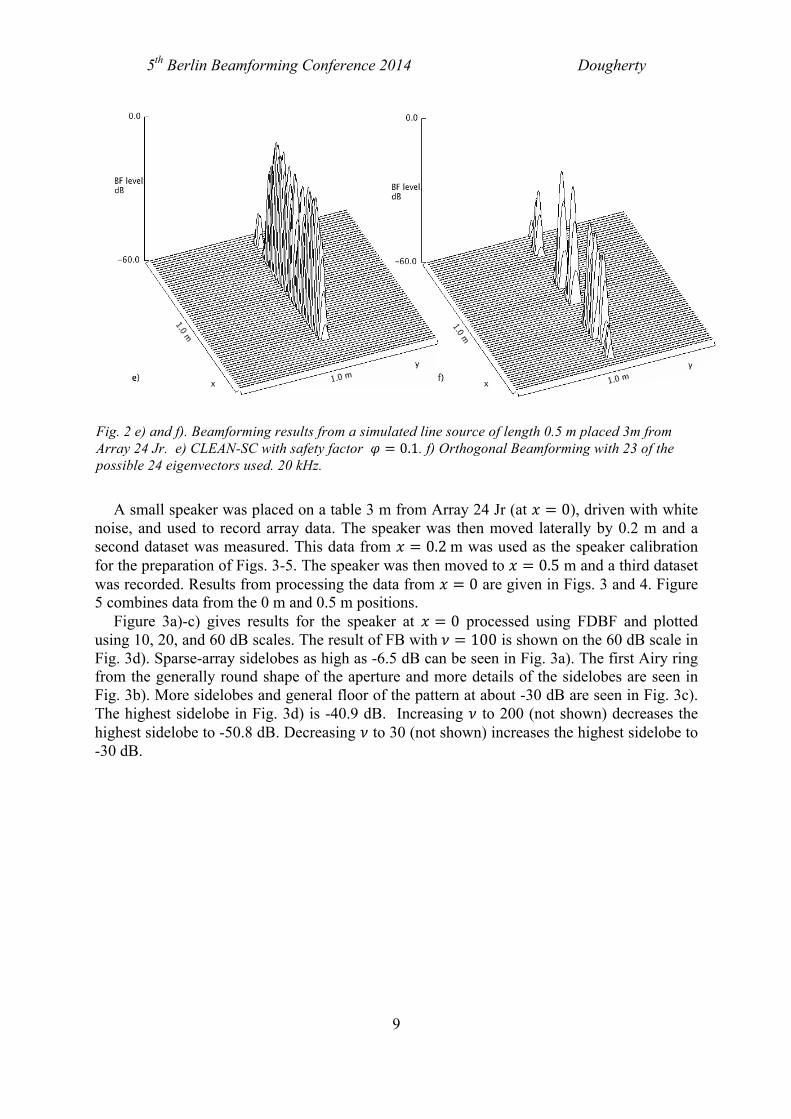
A small speaker was placed on a table 3 m from Array 24 Jr (at ! ! !), driven with white

noise, and used to record array data. The speaker was then moved laterally by 0.2 m and a

second dataset was measured. This data from ! ! !!!!m was used as the speaker calibration

for the preparation of Figs. 3-5. The speaker was then moved to ! ! !!! m and a third dataset

was recorded. Results from processing the data from ! ! ! are given in Figs. 3 and 4. Figure

5 combines data from the 0 m and 0.5 m positions.

Figure 3a)-c) gives results for the speaker at ! ! ! processed using FDBF and plotted

using 10, 20, and 60 dB scales. The result of FB with!! ! !"" is shown on the 60 dB scale in

Fig. 3d). Sparse-array sidelobes as high as -6.5 dB can be seen in Fig. 3a). The first Airy ring

from the generally round shape of the aperture and more details of the sidelobes are seen in

Fig. 3b). More sidelobes and general floor of the pattern at about -30 dB are seen in Fig. 3c).

The highest sidelobe in Fig. 3d) is -40.9 dB. Increasing ! to 200 (not shown) decreases the

highest sidelobe to -50.8 dB. Decreasing ! to 30 (not shown) increases the highest sidelobe to

-30 dB.

Fig. 2 e) and f). Beamforming results from a simulated line source of length 0.5 m placed 3m from

Array 24 Jr. e) CLEAN-SC with safety factor ! ! !!!. f) Orthogonal Beamforming with 23 of the

possible 24 eigenvectors used. 20 kHz.

5th

Berlin Beamforming Conference 2014 Dougherty

10

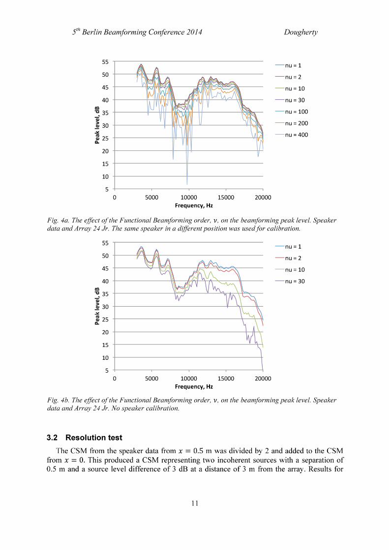
Figure 3 is scaled to show the peak at 0 dB. The effect of ! on the peak level before scaling

is shown in Fig. 4a) for the case with speaker calibration and 4b) for no speaker calibration.

The limiting value of ! in the calibrated case is seen to be close to 200. The peak reduction

effect is smaller at higher frequency, possibly because the array diffraction effects, which

presumably compromise the calibration, are weaker at higher frequency. FB can still be

applied without speaker calibration, but, as indicated in Fig. 4b) the useful value of ! is more

limited. Fig. 4b) suggests that of ! can be 30 or possibly higher for frequencies up to 12 kHz,

but at higher frequency ! should be constrained to values less than 30 in the case with no

calibration. In contrast with the calibrated case, the peak level falls off faster with ! at high

frequency. This may be because there are phase and amplitude errors in the microphones, and

such errors are more important at high frequency. It should be noted that the electrets in Array

24 Jr have considerable variation in sensitivity between them. This should be viewed as nearly

a worst-case array to use without calibration. A worse case would be to mount the

microphones on wobbly stands and fail to measure their exact locations.

Fig. 3. Beamforming at 18 kHz for a speaker located 3 m from Array 24 Jr. a) FDBF on a 10 dB scale.

b) FDBF on a 20 dB scale. c) FDBF on a 60 dB scale. d) Functional Beamforming with ! ! !"" on a

60 dB scale. Speaker calibration was applied using the same speaker in a different location.

5th

Berlin Beamforming Conference 2014 Dougherty

12

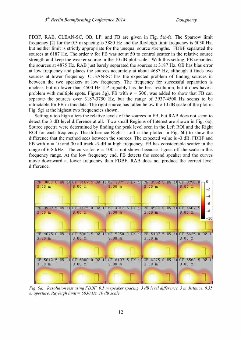
FDBF, RAB, CLEAN-SC, OB, LP, and FB are given in Fig. 5a)-f). The Sparrow limit

frequency [2] for the 0.5 m spacing is 3880 Hz and the Rayleigh limit frequency is 5030 Hz,

but neither limit is strictly appropriate for the unequal source strengths. FDBF separated the

sources at 6187 Hz. The order ! for FB was set at 50 to control scatter in the relative source

strength and keep the weaker source in the 10 dB plot scale. With this setting, FB separated

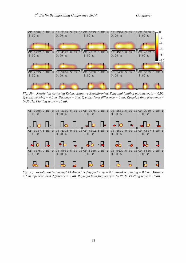
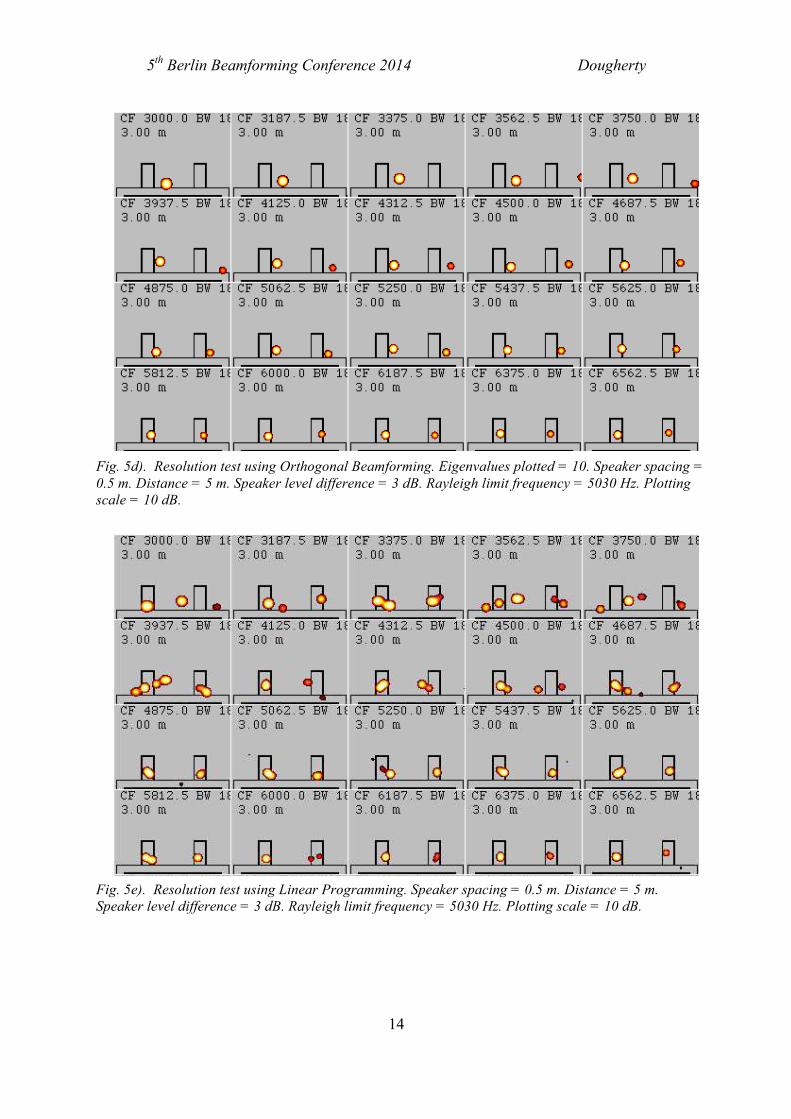
the sources at 4875 Hz. RAB just barely separated the sources at 3187 Hz. OB has bias error

at low frequency and places the sources accurately at about 4687 Hz, although it finds two

sources at lower frequency. CLEAN-SC has the expected problem of finding sources in

between the two speakers at low frequency. The frequency for successful separation is

unclear, but no lower than 4500 Hz. LP arguably has the best resolution, but it does have a

problem with multiple spots. Figure 5g), FB with ! ! !"", was added to show that FB can

separate the sources over 3187-3750 Hz, but the range of 3937-4500 Hz seems to be

intractable for FB in this data. The right source has fallen below the 10 dB scale of the plot in

Fig. 5g) at the highest two frequencies shown.

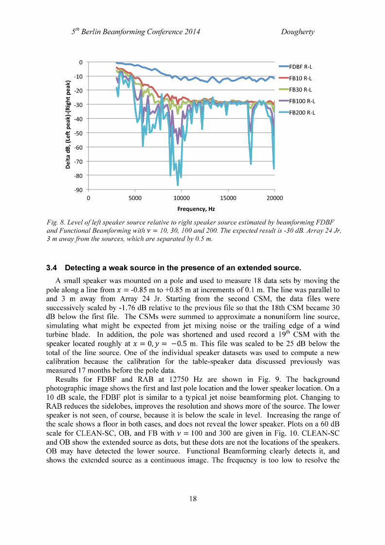
Setting ! too high alters the relative levels of the sources in FB, but RAB does not seem to

detect the 3 dB level difference at all. Two small Regions of Interest are shown in Fig. 6a).

Source spectra were determined by finding the peak level seen in the Left ROI and the Right

ROI for each frequency. The difference Right - Left is the plotted in Fig. 6b) to show the

difference that the method sees between the sources. The expected value is -3 dB. FDBF and

FB with ! ! 10 and 30 all track -3 dB at high frequency. FB has considerable scatter in the

range of 6-8 kHz. The curve for ! ! !"" is not shown because it goes off the scale in this

frequency range. At the low frequency end, FB detects the second speaker and the curves

move downward at lower frequency than FDBF. RAB does not produce the correct level

difference.

Fig. 5a). Resolution test using FDBF. 0.5 m speaker spacing, 3 dB level difference, 5 m distance, 0.35

m aperture. Rayleigh limit = 5030 Hz. 10 dB scale.

5th

Berlin Beamforming Conference 2014 Dougherty

13

Fig. 5b). Resolution test using Robust Adaptive Beamforming. Diagonal loading parameter, ! ! !!!"!

Speaker spacing = 0.5 m. Distance = 5 m. Speaker level difference = 3 dB. Rayleigh limit frequency =

5030 Hz. Plotting scale = 10 dB.

Fig. 5c). Resolution test using CLEAN-SC. Safety factor, ! ! !!!! Speaker spacing = 0.5 m. Distance

= 5 m. Speaker level difference = 3 dB. Rayleigh limit frequency = 5030 Hz. Plotting scale = 10 dB.

5th

Berlin Beamforming Conference 2014 Dougherty

14

Fig. 5d). Resolution test using Orthogonal Beamforming. Eigenvalues plotted = 10. Speaker spacing =

0.5 m. Distance = 5 m. Speaker level difference = 3 dB. Rayleigh limit frequency = 5030 Hz. Plotting

scale = 10 dB.

Fig. 5e). Resolution test using Linear Programming. Speaker spacing = 0.5 m. Distance = 5 m.

Speaker level difference = 3 dB. Rayleigh limit frequency = 5030 Hz. Plotting scale = 10 dB.

5th

Berlin Beamforming Conference 2014 Dougherty

15

Fig. 5f). Resolution test using Functional Beamforming. Order ! ! !"!!Speaker spacing = 0.5 m.

Distance = 5 m. Speaker level difference = 3 dB. Rayleigh limit frequency = 5030 Hz. Plotting scale =

10 dB.

Fig. 5f). Resolution test using Functional Beamforming. Order ! ! !""!

5th

Berlin Beamforming Conference 2014 Dougherty

17

Fig. 7. Beamforming to detect a weak source (-30 dB) located 0.5 m from the stronger source at a

distance of 3 m using Array 24 Jr. Left to right: FDBF, Robust Adaptive Beamforming, CLEAN-SC,

Orthogonal Beamforming, and Functional Beamforming.

5th

Berlin Beamforming Conference 2014 Dougherty

19

individual speakers of the line. Increasing ! reduces the sidelobes. Higher frequency results

(25 kHz) are shown in Fig. 11, but the individual speakers are still not resolved.

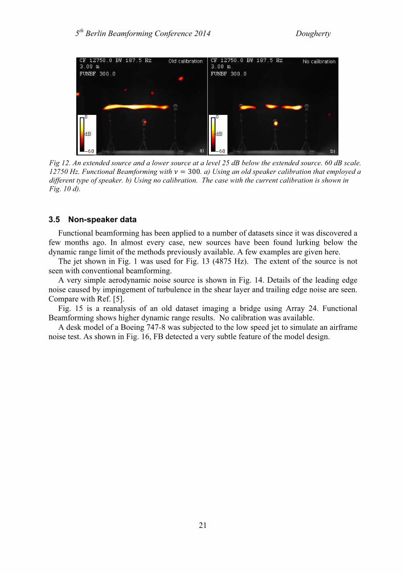
The effect of calibration is explored in Fig. 12, which gives the FB results with ! ! 300

using a) the old calibration (which is also a different speaker type) and b) no calibration. The

results are degraded compared with Fig 10d), but the lower speaker is still seen.

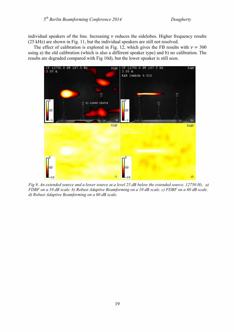
Fig 9. An extended source and a lower source at a level 25 dB below the extended source. 12750 Hz. a)

FDBF on a 10 dB scale. b) Robust Adaptive Beamforming on a 10 dB scale. c) FDBF on a 60 dB scale.

d) Robust Adaptive Beamforming on a 60 dB scale.

5th

Berlin Beamforming Conference 2014 Dougherty

20

Fig. 10. An extended source and a lower source at a level 25 dB below the extended source. 60 dB

scale. 12750 Hz. a) CLEAN-SC. b) Orthogonal Beamforming. c) Functional Beamforming with

! ! !"". d) Functional Beamforming with ! ! !"".

Fig. 11. An extended source and a lower source at a level 25 dB below the extended source. 60 dB

scale. 25 khz Hz. a) FDBF . b) Functional Beamforming with ! ! !"".

5th

Berlin Beamforming Conference 2014 Dougherty

21

3.5 Non-speaker data

Functional beamforming has been applied to a number of datasets since it was discovered a

few months ago. In almost every case, new sources have been found lurking below the

dynamic range limit of the methods previously available. A few examples are given here.

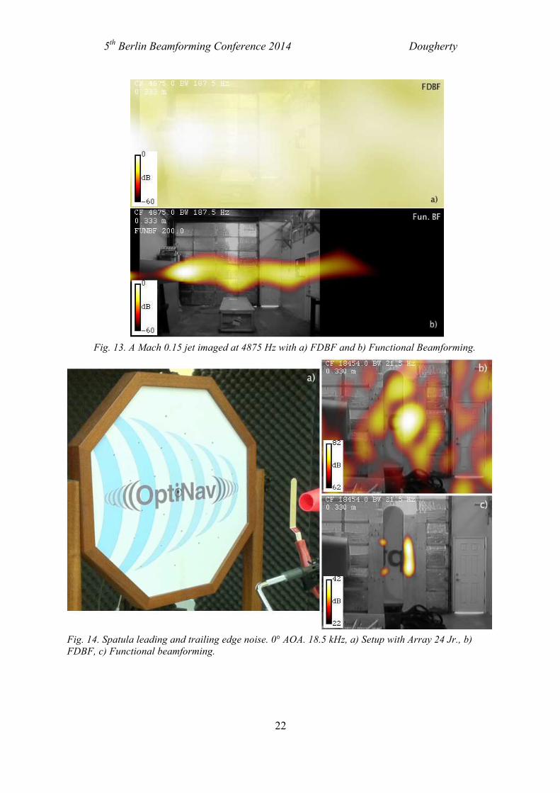
The jet shown in Fig. 1 was used for Fig. 13 (4875 Hz). The extent of the source is not

seen with conventional beamforming.

A very simple aerodynamic noise source is shown in Fig. 14. Details of the leading edge

noise caused by impingement of turbulence in the shear layer and trailing edge noise are seen.

Compare with Ref. [5].

Fig. 15 is a reanalysis of an old dataset imaging a bridge using Array 24. Functional

Beamforming shows higher dynamic range results. No calibration was available.

A desk model of a Boeing 747-8 was subjected to the low speed jet to simulate an airframe

noise test. As shown in Fig. 16, FB detected a very subtle feature of the model design.

Fig 12. An extended source and a lower source at a level 25 dB below the extended source. 60 dB scale.

12750 Hz. Functional Beamforming with ! ! !"". a) Using an old speaker calibration that employed a

different type of speaker. b) Using no calibration. The case with the current calibration is shown in

Fig. 10 d).

5th

Berlin Beamforming Conference 2014 Dougherty

22

Fig. 14. Spatula leading and trailing edge noise. 0° AOA. 18.5 kHz, a) Setup with Array 24 Jr., b)

FDBF, c) Functional beamforming.

Fig. 13. A Mach 0.15 jet imaged at 4875 Hz with a) FDBF and b) Functional Beamforming.

5th

Berlin Beamforming Conference 2014 Dougherty

23

Fig. 15. Noise from a double deck bridge. Sound from traffic on the lower (express lanes) deck reflects

from the bottom of the upper deck. Array 24. 2.8 kHz. a) FDBF, b) Functional beamforming.

5th

Berlin Beamforming Conference 2014 Dougherty

24

Fig. 16. Functional Beamforming of Airframe noise from a desk model of a Boeing 747-8. The spots

near the leading edge of the wing root are from tiny depressions representing the air cycle machine

inlets.

4 CONCLUSIONS

Functional Beamforming (BF) is a simple modification of conventional Frequency Domain

Beamforming that offers much higher dynamic range than FDBF or any other beamforming

method to the author’s knowledge. Dynamic range of more than 30 dB has been demonstrated

over a substantial bandwidth using a 24-element array with inexpensive microphones. FB has

no significant impact on computing time or other resources. It depends on an order, !, that

connects it with FDBF (! = 1) and even MVDR (! = -1). The resolution of FB is better than

that of FDBF, but not quite as sharp as Robust Adaptive Beamforming or Linear

Programming. Unlike deconvolution methods, it shows continuous source distributions as

continuous images. There is a proof of its quantitative nature based on the theory of matrix

monotone functions. If the steering vector is correct, FB will never give a result that is lower

than the actual source strength. Furthermore, the beamform map steadily decreases as ! is

increases. The sidelobes gradually disappear and the main lobes become somewhat narrower.

At first glance, this would seem to suggest that that the exact answer is obtained in the limit as

! ! !, but this is unproven and seems too good to be true. In practice, errors in array

calibration or the propagation model will cause at least small errors in the computed steering

vectors, and this will limit the useful range of !. Experience to date suggests that an

uncalibrated array can support ! up to 30 and a well-calibrated one can handle ! in the

hundreds.

REFERENCES

[1] Brooks, T.F. and W.M. Humphreys, Jr. “A Deconvolution Approach for the Mapping of

Acoustic Sources (DAMAS) determined from phased microphone arrays,” AIAA Paper

2004-2954, 2004.

[2] Dougherty ,R.P., R.C. Ramachandran and G.Raman,"Deconvolution of Sources in

Aeroacoustic Images from Phased Microphone Arrays Using Linear Programming,"

R.P., AIAA Paper 2013-2210, Berlin, Germany, 2013.

5th

Berlin Beamforming Conference 2014 Dougherty

25

[3] P. Sijtsma. “CLEAN based on spatial source coherence.” Int. J. Aeroacoustics, 6, 357–

374, 2007.

[4] Dougherty, R.P., “Source Location with Sparse Acoustic Arrays; Interference

Cancellation,” CEAS-ASC Workshop, "Wind Tunnel Testing in Aeroacoustics" DNW,

Noordoostpolder, the Netherlands, November 5-6, 1997.

[5] Sarradj, E., “A fast signal subspace approach for the determination of absolute levels

from phased microphone array measurements,” Journal of Sound and Vibration 329,

1553–1569, 2010.

[6] Cox, H., R. M. Zeskind, and M. M. Owen, “Robust adaptive beamforming,” IEEE Trans. Acoust., Speech, Signal Process., 35 (10), 1365–1376, 1987.

[7] Johnson, D. H. and Dudgeon, D.E., Array Signal Processing: Concepts and Techniques

Prentice-Hall, 1993.

[8] Huang X., L. Bai, I.Vinogradov, and E. Peers, “Adaptive beamforming for array signal processing in aeroacoustic measurements,” J Acoust Soc Am. 131(3), 2152-61, 2012.

[9] Underbrink, J.R., and R.P. Dougherty, “Array design for non-intrusive measurement of

noise sources,” Noise-Con 96, Bellevue, WA, 1996.

[10] Bhatia, R., Matrix Analysis (Graduate Texts in Mathematics), Springer, 1997.

[11] Witkowski, A., “A new proof of the monotonicity of power means,” Journal of Inequalities in Pure and Applied Mathematics, Vol. 5, Issue 1, Article 6, 2004.