Functional Data Analysis of Hydrological Data in the

Potomac River Valley

Aaron Zelmanow

American University

October 31, 2012

Acknowledgement to:

Dr. Inga Maslova - American University

Dr. Andres Ticlavilca - Utah State University

1 Abstract

Flooding and droughts are extreme hydrological events that affect the United States

economically and socially. The severity and unpredictability of flooding causes billions of

dollars in damage and catastrophic loss of life. In this context, there is an urgent need

to build a firm scientific basis for adaptation by developing and applying new modeling

techniques for accurate streamflow characterization and reliable hydrological forecasting.

The goal is to use numerical streamflow characteristics in order to explore the ability to

classify, model, and estimate the likelihood of extreme events in the eastern United States,

mainly the Potomac River. Functional data analysis techniques are used to study yearly

streamflow patterns, with the extreme streamflow events characterized via functional

1

principal component analysis. These methods are merged with more classical techniques

such as cluster analysis, classification analysis, and time series modeling. This exploratory

analysis features models and forecasting methods that, while not comprehensive, are the

foundation for future study.

2 Introduction

Functional data analysis is a relatively new and novel approach to statistical analysis. The

conversion of discrete data points to functional objects for the purpose of analysis began

in the 1990’s and has only been used for a little over a decade in the field of hydrology.

To establish a foundation for the potential of functional data analysis within the field of

hydrology the work of Suhaila et al. (2011) was utilized. Their research utilized functional

data analysis to compare rainfall between regions within Peninsular Malaysia and provided

the groundwork for the use of functional data analysis and smoothing techniques that were

utilized in the study of the Potomac River hydrological data. Additionally the merging

of clustering techniques and functional data analysis were identified and discussed by

Huzurbazar and Humphrey (2008) in their study of subglacial water flow.

To merge the techniques of functional data analysis and time series analysis, the

mortality and fertility rate analyses of Chiou and Muller (2009) and Hyndman and Ullah

(2006) were referenced. The work presented by their papers provided information into

the process of converting data into functional data, the benefits of smoothing techniques

and the resulting fit of functional data into time series ARIMA models. This analysis was

able to expand these techniques by reviewing various aspects of functional data within

the time series analysis.

2

3 Data Description

The data set used to model the streamflow is from the Potomac River and is measured

in cubic feet per second. The United States Geological Survey (USGS) has positioned

sensors at intervals along the river and has taken monthly readings from 1931 to 2012. A

graphic of the time series for the first five years of data is found in Figure 1. The survey

site used for this analysis is the Little Falls Pump Station on the Potomac River, site

1646500 1.

Little Falls Pumping Station is a dam and pumping station in Maryland used to pro-

vide a water supply for Washington DC. Water pumped from the station is extracted

upriver of the Chesapeake and Ohio Canal and travels downhill to purification plants

for the nation’s capital. The sensors at the pumping station are affected by a multi-

tiude of man-made and natural factors that effect the predictability of stream flow. The

river provides water for households and irrigation and supports industrial and economic

development2. Additionally, natural factors that increase the variability in streamflow in-

clude melting snow and ice, direct precipitation and stream gradient of both the identified

river and other connecting water sources. The physical proximity of the Potomac River

to both the eastern coast of the United States and the Shenendoah Mountains creates

highly variable amounts of precipitation.

As a gaining river, the Potomac River is increases in streamflow with movement away

from its origin. As the most southernly of the sensors on the Potomac River, the Little

Falls Pumping Station is furthest from the origin but subject to the maximum amount of

increase in streamflow. Combining this with the volatility associated with the man-made

and natural factors discussed, the variability in streamflow through time is maximized at

the pumping station and there is greater potential for building a streamflow model that

1http://ida.water.usgs.gov2www.nature.org/ourinitiatives/

3

can be utilized across a wide range of rivers and locations.

To fit the data using functional data analysis, the available data had to be reduced by

a total of seven months. The first three months of 1931 and the first four months of 2012

were removed to satisfy the R-Statistical Software requirement of all functional curves

being the same length. The length chosen was twelve months and is analyzed as January

1st to December 31st, ensuring that the time of year containing the greatest amount of

activity, Spring and Fall, are centered within each function.

4 Exploratory Analysis

The graphic of the stream flow data in Figure 2 displays 81 years of streamflow data

as a matrix plot, overlayed on a 12 month axis. As determined by NOAA 3, flooding

at the Little Falls Pumping Station on the Potomac River (site 1646500) is categorized

as major, moderate, minor and none; the respective color coding representing flooding

magnitude is red, purple, navy and sky blue. During the exploratory phase there were two

identified periods of increased streamflow, once the spring and again in the fall, with floods

occurring multiple times within some years. A component of the analysis is to determine

if a year with a flood event can be identified prior to its occurrence. To meet this end,

flood severity coding is applied according to the the greatest flood event occurring within

each year.

Flooding along the Potomac river is determined as the crest, measured in feet, of the

water. A major challenge in modeling the data has been to reconcile the flood events,

measured in feet, and the data used to create the models, being streamflow measured in

cubic feet per second. A visual inspection of the data in Figure 2 indicates that there

is a connection between the two measurements, warranting further analysis and model

3www.erh.noaa.gov

4

development.

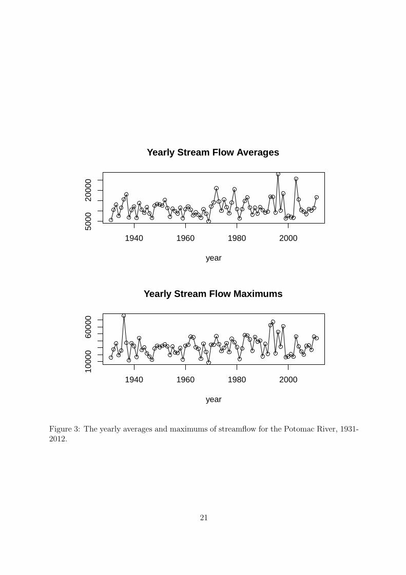
Figure 3 displays the stream flow averages and maximums over the 81 year record.

From this graphic there are indicators that the average yearly stream flow has increased

in variability over time. Additionally, there are also visual indicators that show that the

yearly stream flow maximums have increased in both magnitude and variability. This

initial assessment is used cautiously during the exploratory phase. Natural factors such

as weather patterns, sediment levels and erosion of the river banks change over time,

meaning that the amount of stream flow in one year may lead to flooding, but the same

streamflow under different conditions in another year may not lead to the same flood

severity. Additionally, the definitions of flooding and scientific advances in how stream-

flow is measured have changed over time, effecting how flood events are determined and

categorized.

5 Functional Data Analysis

Functional data analysis is intended to allow observed data to be treated as a continuum of

information rather then a sequence of individual observations. In the case of streamflow,

as is often the case with functional data, the discrete data is referenced as an observation

at a point in time. The conversion of discrete data points to functional data allows it to

be modeled in a manner that integrates the structure of the data as a function whereby

it can be analyzed and modeled using mathematical functions such as derivatives. In

order to successfully use mathematical properties on the functional data, a smoothing

parameter is added that assumes that observation yj and yj+1 are linked and unlikely to

differ substantially. In the context of streamflow, a smoothing parameter would assume

that streamflow on January 1st would likely not differ much from streamflow on January

2nd, or in a more granular sense, streamflow at 10:00am is unlikely to differ greatly from

5

11:00am. When smoothing parameters are added in the functional analysis, the error, or

residual, between the model and raw data is increased in favor of a more easily interpreted

model. A negligible smoothing parameter, virtually zero, was used in this analysis to

maximize the use of available information, which is of particular importance considering

that there is only one observation available per month, a relatively small amount of data

in the realm of functional data analysis. The notation used to express observational error

or residual, ϵ is:

(5.1) yj = x(tj) + ϵj ȷ = 1, 2, ..., 12

where yj represents the value of observation, j, composed of the value at the observation

plus the additional error or noise.

The fundamental component of functional data is the basis function, a mathematical

description of the data within a confined space. At its essence, the basis functions act as

building blocks with which functions are built and parameters easily estimated using a

matrix of coefficients. The data was transformed into functional objects with the intent

of minimizing the residual difference between the basis objects and the actual data. A set

of functional building blocks ϕk, k=1,...,K, or basis functions, are combined linearly such

that the function x(t) may be expressed in mathematical notation as the basis function

expansion:

(5.2) x(t) = ΣKk=1ckϕk(t) = cTϕ(t)

The parameters c1, c2,..., ck are the coefficients of expansion, cT is equal to the vector

of K coefficients and ϕ(t) = (ϕ1,(t),...ϕK(t)) is a vector of length K containing the basis

functions (Ramsay and Silverman (2005), page 44).

6

While there are numerous basis systems that can be used, the Fourier and bspline

basis systems were deemed most appropriate for the analysis. The Fourier system is

the usual choice for periodic functions, or functions displaying sinusoidal tendencies, and

the bspline system being the preferred system for non-periodic functions. Other basis

functions, such as constant or monomial systems were disregarded as visual assessment

of the data indicates streamflow is neither monomial nor constant in nature.

Figure 4 shows the data modeled using the Fourier basis system. The Fourier basis

system relies on the data being separated by breaks, within which the data is modeled

using sinusoidal functions. Visual assessment of the data presented several issues which

led to a rejection of the model. The first issue identified with the Fourier system is that

numerous yearly observations are forced to take on negative stream flow values. Secondly,

the data is coerced into taking the same value at both ends of the function, meaning that

January 1st and December 31st are assigned the same streamflow value, increasing the

residual error between the function and actual data at the beginning and end of each year.

This non-uniform increase in residual error led to questions regarding the independence

of observations, and ultimately the decision to not use the Fourier basis system.

The data was also modeled using the bspline basis system, where the relationship

between basis functions, interior knots and the order of the data become paramount

in creating a model that sufficiently represents the data and allows for computational

analysis. The relationship between the parameters is described in the equation (Ramsay

et al. (2009), Page 35):

(5.3) # of basis functions = order +# of interior knots

Where the number of basis functions is determined by the order of the polynomial seg-

ments and the number of interior knots or breakpoints. In order for the model to be

7

optimized in its computational power, the order must be equal to three or greater. With

an order of three, analysis of the velocity and acceleration can be performed using the

first and second derivative of the data. The streamflow data is best represented yearly

due to annual weather patterns. With one streamflow observation taken per month, 11

interior knots were selected, allowing for one observation for each basis function. Thus,

the total number of basis functions selected is 14. Other parameter arrangements were

tested but ultimately led to either a loss in power, with the order being reduced, or the

disregard for data by coercing multiple observations into a single break, a result of de-

creasing the number of interior knots. Figure 5 displays the basis functions and model

using the selected bspline basis system.

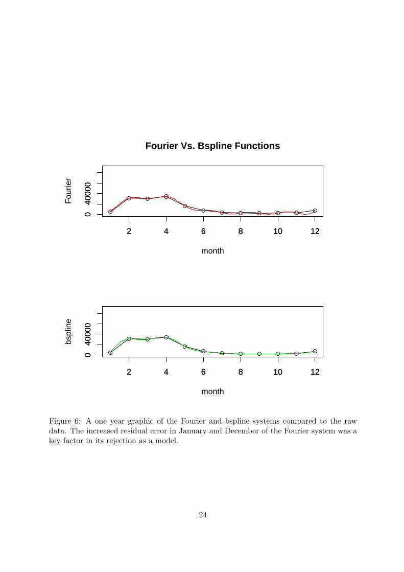
When comparing the Fourier and bspline models, two methods determined the best

model fit, visual assessment and calculation of the root mean square residuals. Figure 6

offers a one year comparison of the basis systems compared to the raw data, Fourier and

bspline respectively. The root mean square residual of the Fourier basis system is 851.54,

while the bspline basis system root mean square residual equals 554.53. Both the visual

assessment and computation of residuals are in agreement that the bspline basis system

is the best fitting model.

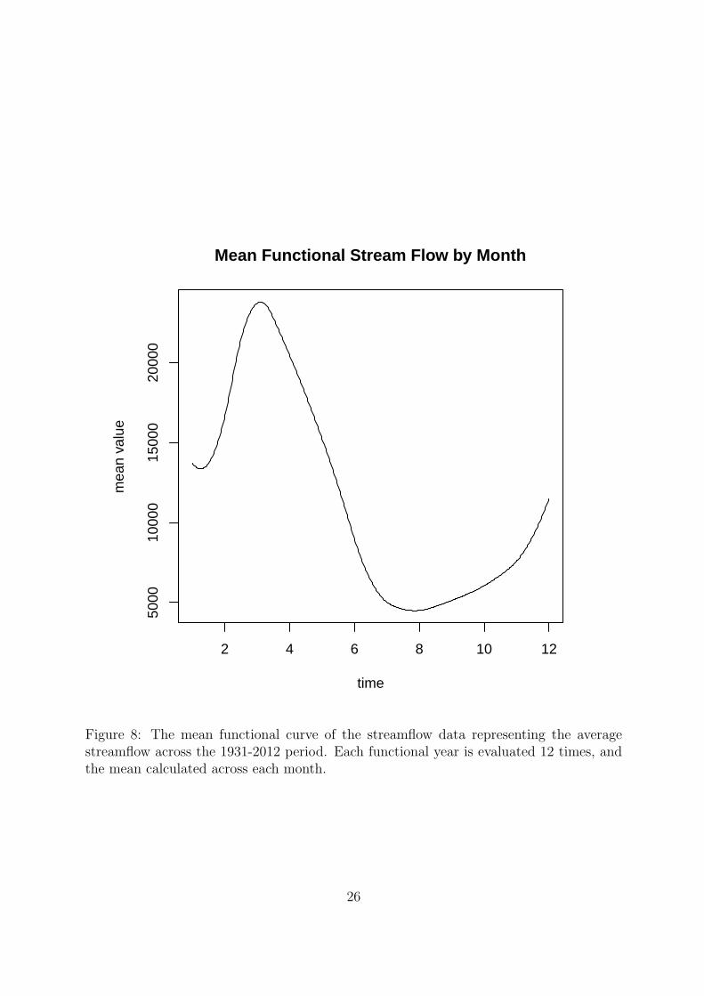
With the bspline model in place, the five year graphic, figure 7, displays the raw

data and functional data of the Potomac River from 1931-1935. The mean functional

streamflow was also obtained as figure 8 displaying the general shape and form of the

streamflow through the year, created by obtaining the average across the 81 years of

observations. We see the pattern of average streamflow maximizing in early Spring and

minimizing in the summer which is intuitive when snow melt and typical rain patterns in

the region are considered.

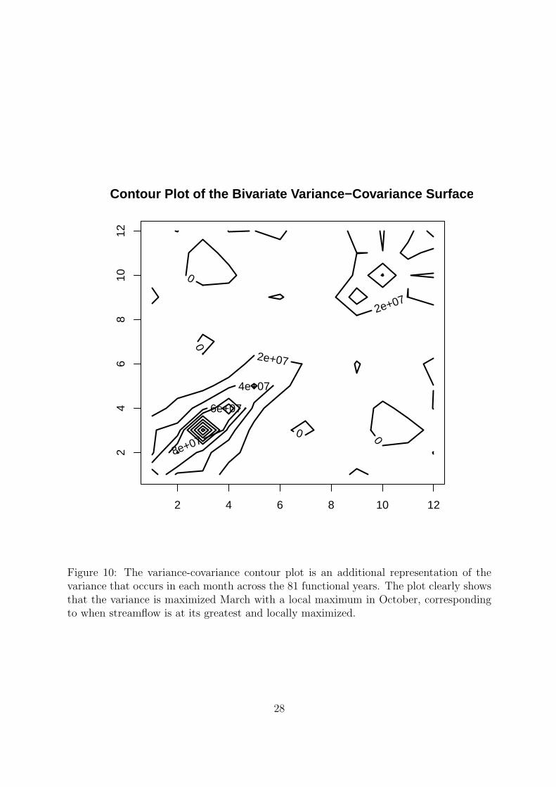
Additionally, with the model in place, the variance-covariance perspective plot in

figure 9 and variance-covariance contour plot in figure 10 were generated to provide a

8

representation of the variance in monthly stream flows from year to year. The greatest

variance occurs in March, with November being a month with a localized increase in

variance. This indicates that while the stream flow follows a basic pattern every year, the

timing of pattern changes and the amount of increase in streamflow have a much greater

variance when the annual streamflows are at their highest levels.

Lastly, the functional data enabled the computation of derivatives, used to further the

analysis and modeling of the streamflow data. Figure 11 displays a four-piece graphic

that displays the functional data, residuals, first and second derivatives of the year 1931.

With this information, modeling of both the velocity and acceleration of streamflow can

be incorporated into the analysis.

6 Cluster Analysis

In order to classify flood events using streamflow data both the number of evaluated points

in time and the registration, or occurrence, of significant events had to be considered.

When using the functional data each functional observation, or year, has the ability to be

evaluated at designated intervals. In most cases, the functions are evaluated monthly to

correspond to the monthly raw data readings, but in scenarios when more granularity is

beneficial the functions are evaluated 100 times over the course of an observational year.

Additionally, the functional data underwent a continuous registration process in which

the functional observations were aligned with a target curve using continuous criterion

such as maxima, minima, velocity and acceleration. To align the functions a warping

function, or smooth increasing transformation, is applied to each observational function.

Figure 12 displays the registered curves and warping functions.

The characteristics chosen to undergo cluster analyses is the first and second deriva-

tives of the functional data to determine if the velocity or acceleration of streamflow could

9

be used to cluster functional observations into groups corresponding to flood severity. The

registered curves and warping functions were also selected to undergo cluster analyses as

shared flooding traits may become more apparent in the registration process. The regis-

tered curves yielded largely the same classification results as the unregistered functional

data and therefore only one is presented.

The initial clustering method used the Euclidean distance of the functional data and

registered functional data. In order to calculate the Euclidean distance, each yearly

function was evaluated at 100 points in time. The distance between the corresponding

evaluated points in each year was then plotted with colors coded to indicate the greatest

flood event within the observed year. While unable to produce clusters that matched the

flood severity categorization provided by NOAA, a dendrogram of the Euclidean distance

method captured almost all of the non-flood years within a single cluster. The results

were ultimately disregarded as the three types of flood events were categorized into seven

different clusters.

The k-means method of clustering was also used to attempt a classification of the data.

The k-means clustering method uses algorithmic computations to partition data into k-

clusters in which each observation is assigned its cluster according to its mean and the

mean of the clusters. The k-means method was used to test the the registered functional

data, warping functions and streamflow velocity and acceleration. Figure 13 is a graphic

representation of the k-means process, with the color coding representing the flood events

and the icons representing the clusters derived in the k-means process. Of the attributes

tested the warping function clustering was the most successful as it correctly clustered the

majority of non-flood years, but was ultimately rejected as it failed to create clustering

that matched the three flood events.

A PAM analysis was also conducted using clustering around medoids, or clustering

based on dissimilarity, resulting in an more robust version of the k-means method. Fig-

10

ure 14 shows the results of the analysis, which largely failed to accurately classify the data

in flood severity categories. In this analysis, the registered data captured the majority

of non-flood events in a cluster, but failed to capture the rest of the data in accurate

clusters. The warping functions, velocity and acceleration of the registered data failed to

cluster the data in a meaningful manner.

Finally, the registered data, warping functions, first derivative and second derivative

underwent a classic cluster analysis whereby the data was plotted using the same color and

icon coding as above. Additionally, dendrograms were created in which the classification

trees were coerced into creating four clusters, each representing the severity of flood events

occurring within the year. Regardless of the clustering method; single, complete, Ward or

average, the functional characteristics all failed to cluster the data accurately. Virtually all

cluster techniques yielded only 24-28 correct classifications, not enough to be considered

significant findings.

7 Functional Principal Component Analysis

A principal component analysis is a procedure that transforms a number of potentially

correlated variables into a smaller number of uncorrelated variables called principal com-

ponents. The first principal component accounts for the most variability in the data and

each successive component accounts for a decreasing amount of variability. The principal

components are comprised of eignevalues, η, and eigenfunctions or harmonics, ξ. The

analysis searches for the harmonic of the equation below that has the largest possible

variance (Ramsay and Silverman (2005), Page 100)

(7.1) ρξ =

∫ξ(t) xi(t) dt

11

The eigenvalue variance associated with a harmonic is the value of:

(7.2) η = maxξ

[Σiρ2ξ (xi)], subject to

∫ξ2(t) dt = 1

When considering how an observation is deconstructed using the principal componentscores, or eigenvalues, and harmonics the following equation provides an applied formulaicmethod:

(7.3) xt = µt + Σ∞j=1γj ξj(t)

xt = observation x at time tµt = mean of the dataγj = principal component score vectorξj(t) = jth eigenfunction or harmonic

Using a Scree test, four principal components were chosen as the most efficient number

to represent the data. The four principal components displayed in Figure 15 account for

76% of the variation in the data. The harmonics used to create the principal components

are in figure 16. The first principal component captures the seasonal variation of the

streamflow, largely rising in March and minimizing in August. The greatest amount of

variation captured is in the amount of streamflow that occurs at the maximum. The

second principal component accounts for the variation that occurs from the streamflow

variability during late spring, summer and winter months. The third principal component

captures the shift in the timing of the early spring peak flows, or changes from winter to

spring. The fourth principal component highlights the increase in streamflow in the early

spring months.

A rotated principal component was considered using the varimax function. Ultimately,

the procedure was not used as the analysis incorporates a penalization for harmonic ac-

celeration. The varimax procedure, capturing the variation in streamflow, is estimated by

12

penalizing the squared deviations in harmonic acceleration as measured by the differential

operator. If the stream flow variation was purely sinusoidal, the yearly curves would be

exactly zero. The reasoning for this not being used is that the penalty increases with the

higher order harmonics, distorting the interpretation of the latter principal components.

With a functional principal component analysis in place using four principal compo-

nents, the plot in figure 17 was created to determine if there is any correlation between

the variation seen in the first four principal components and the years where floods oc-

curred. In the scatterplot on the axis of the first two principal components outliers were

identified by the most extreme observations dependent on their distance from the mean.

Observations with a first principal component greater then 10,000 and with a second prin-

cipal component greater then 20,000 were determined to be outliers. Of the 15 years that

were identified to be outliers there were; three years with major floods, seven years with

moderate floods, four years with minor floods and only one year where no flooding at all.

The range of types of floods found to be outliers and the fact that many flood years were

not considered outliers indicates that there is not a strong enough relationship between

the principal components of stream flow to make determinations or predictions regarding

flood events without additional information or analysis techniques.

8 Forecasting Models

Median Testing Model

(8.1) X(t+1) = µ+ Σ4j=1γ(t+1)ξj(t)

Xt = observation x at time tµt = mean of the dataγt+1 = nested median of principal component scoresξj(t) = jth eigenfunction or harmonic

13

Mean Testing Model

(8.2) X(t+1) = µ+ Σ4j=1β(t+1)ξj(t)

Xt = observation x at time tµt = mean of the dataβt+1 = nested mean of principal component scoresξj(t) = jth eigenfunction or harmonic

AR(1) Testing Model

(8.3) X(t+1) = µ+ Σ4j=1α(t+1)ξj(t)

Xt = observation x at time tµt = mean of the dataαt+1 = nested ar(1) forecast of principal component scoresξj(t) = jth eigenfunction or harmonic

RMSE (Root Mean Square Error) Formula for Forecasting

(8.4) MSRE =1

mΣm

j=1

√Σy

i=1(fi − di)2

m = # of months in a forecasting year, typically twelvey = # of years in forecastfi = A matrix of forecast values with y columns and m rowsdi = A matrix of true values with y columns and m rows

9 Forecasting as a Time Series

Using ACF (autocorrelation function) and PACF (partial autocorrelation function) anal-

yses, the registered functional data, warping functions, principal components, and first

and second derivatives were tested to determine if there was a SARIMA (seasonal au-

toregressive integrated moving average) model that explains the variation in the data. Of

the characteristics tested, no strong pattern was identified, but the principal component

scores did exhibit a slight seasonal component that warranted further analysis.

Without a specific SARIMA model with which to analyze and forecast the principal

component scores, the AR(1) or first order autogregressive process was used as it is the

14

archetypical time series process. To determine the ability for the principal components

to be used in the forecasting process, a 71 year training set and 10 year testing set was

used. The forecasts were nested, so that each year in the forecast contained not only

the 71 years of the training set, but every subsequent forecast includes the data for all

previously forecasted years. The 10 year training set was used to test the accuracy of the

forecasts to predict streamflow. Using formula 8.4 the root mean square error (RMSE)

of the training set was calculated at 9,437.7. The RMSE of the training set allows for a

baseline calculation which can be used to measure the success of the forecast models.

Formula 8.1 was used in the median forecasting method. The median of the functional

principal component scores for the nested training set was calculated and then multiplied

by the functional principal component harmonics to derive forecasted streamflow values.

This model was compared to the testing set using the RMSE and graphics containing the

historical data, forecasted data and a 95% confidence band. The principal component

analysis was performed uncentered, with the mean included in the analysis, and centered,

with the mean subtracted from the analysis and later added back to the data prior to

forecasting. The uncentered forecast had an RMSE of 8,495.5 and the centered forecasts

had a RMSE of 8,510.3, both perfoming better then the testing set when compared to

the raw data.

Formula 8.2 is the formula used in the mean forecasting method. In this scenario, the

mean of the functional principal component scores for the nested training set was cal-

culated and then multiplied by the functional principal component harmonics to derive

forecasted streamflow values. As with the median forecasting method, formula 8.1, this

model was compared to the testing set using the RMSE and graphics containing the histor-

ical data, forecasted data and a 95% confidence band. The principal component analysis

was also performed centered and uncentered enabling a comprehensive comparison. Both

of the methods peformed better then the testing set with the centered functional princi-

15

pal component analysis leading to a forecast with an RMSE of 8526.2 and the uncentered

functional principal component analysis providing and RMSE of 8,393. While the RMSE

in the forecast performed well, the model was ultimately not used as the uncentered prin-

cipal component analysis yielded principal component scores so close to zero that the

mean was the only information captured for the forecast.

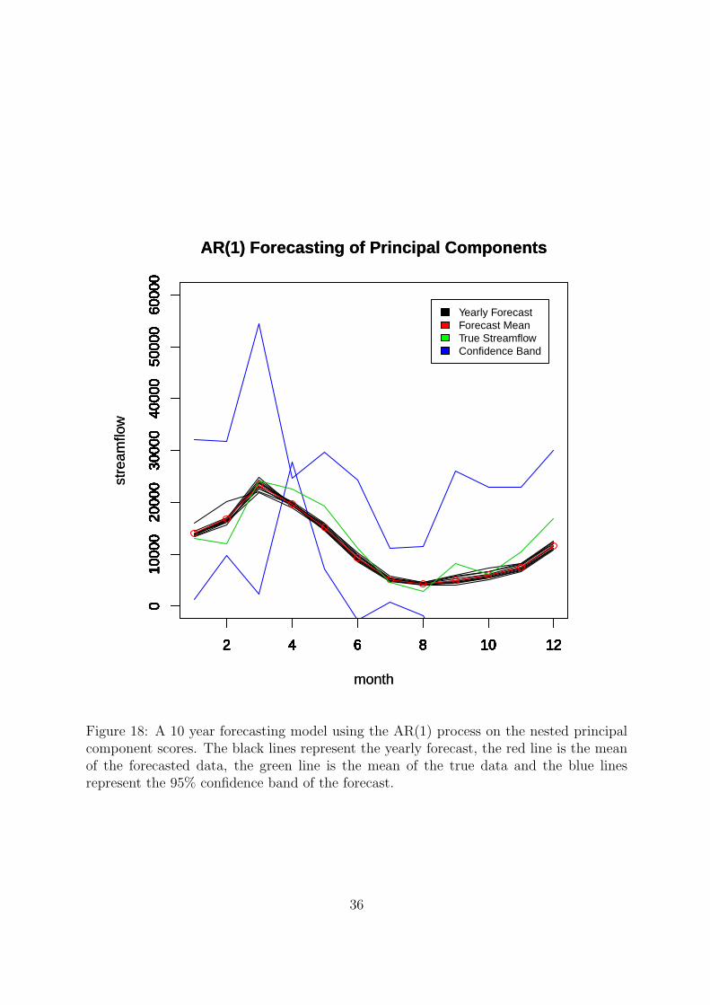
Equation 8.3 is the final, and most successful, forecasting method using a nested AR(1)

model to forecast the functional principal component scores. The principal component

scores were then multiplied by their corresponding harmonics to derive a streamflow

forecast. As with the modeling using the mean and median, the fit of the 10 year forecasted

model was tested using the RMSE and graphics were created that contain the historical

data, forecasted data and a 95% confidence band to determine if the true data lay within

the boundaries of the forecasted model. Also, as with the mean and median modeling,

the forecast was tested twice, once using a centered principal component analysis with

the mean not included and once using an uncentered analysis with the mean included. In

this scenario, the uncentered forecast RMSE is 8,604.4 and the centered forecast, which

outperformed all of the other models, including the training set, with an RMSE of 8,493.

Figure 18 shows the AR(1) forecast model, the black lines indicate the forecasted yearly

streamflow, with the red line representing the mean of all 10 years in the testing set. The

green line represents the mean of the true data in the 10 testing set years, and the black

lines represent the 95% confidence bands. In the graphic it is easy to see that the mean

of the true data lies within the confidence band and does not differ significantly from the

forecasted data. What is difficult to interpret is why the confidence bands have a series of

hierarchical switches in the month of April. When referencing the confidence bands, each

band represents the most extreme hydrological years. The top 97.5% of functional years

has a streamflow that reaches its maximum in March while the bottom 2.5% of functional

years reaches its maximum in April. The shift in time of extreme events, followed by a

16

uniformed steep decline in streamflow are the cause of the flip in confidence bands.

10 Conclusion

The necessity to model and forecast extreme hydrological events is indisputable, and as

flood events continue to occur, the urgency to develop methods of early warning detection

become ever more urgent. The exploratory analysis, models and forecasting methodolo-

gies used in development of this paper reflect what is possible through the use of statistical

analyses in regards to extreme hydrological events. The results found here are a testa-

ment that stand alone traditional methodology does not have enough power to model the

complicated and multifaceted science of streamflow analysis. The most successful aspects

of this analysis were the layered and concurrent use of many statistical tools, such as in

the forecasting method whereby principal component analysis and time series forecasting

methods were merged.

Moving forward, there are numerous attributes that should be introduced. These

models may be more adept when the effects of man are considered. This can be achieved

by reading different sensors along the stream, using adjusted data or adding categorical

variables to the methodology. Additionally, global and local recurring weather patterns

can be introduced to further enhance the accuracy of the model. Finally, the velocity

and acceleration of the streamflow can be analyzed more thoroughly to determine if there

is an evaluatable point prior to flood events where the severity can be determined and

modeled.

17

References

Chiou, J-M. and Muller, H-G. (2009). Modeling hazard rates as functional data for

the analysis of cohort lifetables and mortality forecasting. Journal of the American

Statistical Association, 486, number 1, 572–585.

Huzurbazar, S. and Humphrey, Neil F. (2008). Functional clustering of time series: An

insight into length scales in subglacial flow. Water Resources Research, 44, number

W11420, 1–9.

Hyndman, Rob J. and Ullah, Md. Shahid (2006). Robust forecasting of mortality and

fertility rates: A functional data approach. Computational Statistics & Data Analysis,

51, number 1, 4942–4956.

Ramsay, J. O., Hooker, Giles and Graves, Spencer (2009). Functional Data Analysis with

R and MATLAB. Springer Verlag.

Ramsay, J. O. and Silverman, B. W. (2005). Functional Data Analysis. Springer Verlag.

Suhaila, Jamaludin, Jemain, Abdul Aziz, Hamdan, Muhammad Fauzee and Zin, Wan Za-

wiah Wan (2011). Comparing rainfall patterns between regions in peninsular malaysia

via a functional data analysis technique. Journal of Hydrology, 411, number 1, 197–

2006.

18

050

0015

000

2500

035

000

Five Years of Raw Data

month

stea

mflo

w

1931 1932 1933 1934 1935

Figure 1: Raw data of the Potomac River at the Little Falls Pumping Station site 1646500,1931-1935. Each year is seperated by a horizontal line.

19

1 11

1 1

1 1 1 1 1 1 1

2 4 6 8 10 12

020

000

4000

060

000

Raw Data, Potomac River, 1931

Month

Str

eam

Flo

w

2

22 2

2

2 2 2 2

2

2

2

3 3

3

3

3

3 3

3

33 3 3

4

4

4 4

44

4 4

44

4

45

5

5

5

5

5 5 55

55 5

6 6

6

6

66 6 6 6

66

6

7

7

7

7

7

77

77

7

7

78 88

8 88 8 8

8 8 8

89

9

9 9

99 9 9

9 9 990

0 0

0

0

0

00 0

0

0 0aa

aa

aa a

a a a aab

b

bb

b

bb

b

b

b

b

bc

cc

cc

cc

c c cc

c

d d

d

d d

dd d d

dd

de

ee

e e

e ee

e

ee

ef

ff

f

f f

f ff f f f

g

g

g

gg

g gg g g

gg

hh

hh

h

hh h

h

h h

hi

i

ii

ii

i

ii

ii

ij

j

j

j

j

j

j j

jj

j

j

k

k

k

k

k

k

kk k k k

k

l

l

l

l

l

ll l

ll

l l

m

m

m

m m

m

m m m m mmn n

n

n nn

n n n

nn

no o

o

oo

o

o

o

o o o op

pp

p

p pp

pp p

ppq

q

qq

q qq q q q q

qrr

r rr

r r rr r r r

s ss

ss s

s s ss

ss

tt t

t

t

t

t t t t t tu

u uu

u

uu u u u u

uv

v

v

v

vv

v v v vv

v

ww

w

ww

ww w w w w w

x

x

x

xx

x x x x x xx

yy

y

y

y

y y y y y y yz

z z zz

z z z

z zz

zA A

A

A

A

A AA

AA A

AB

B

B

BB B

B B B BB BC

C C CC C C

CC

C CC

D

D

D

D

DD

DD D D

D DE

E

E

EE E

EE E

EE

E

F

F FF F

F

F

FF

F

F

F

G

G

G

G

G

G

G G G G G

GH

H H

H

HH

H H H H H

HI

I

I

II

II

I

I

I

II

J

JJ J

J JJ J J

J

J J

KK

K K

KK K K K K

K

KL

L

L

L

L

LL

L

L L L

L

M M

M

M MM

M M

M

M

M

M

N

N

N

N

N

NN N N N N NO

O

O

OO

O

OO O O O O

P

P P

P

P

P

PP P P P

PQ

Q

Q

Q

Q

Q

Q Q QQ

Q

Q

R

RR

R

R

R RR

R R R

RS

S

S S SS

S S S S

S

S

T

T T

TT

T T T T TT

TU UU

U

U

U UU

UU

U

UV VV

V

V

VV V V V

V VW W

W

W

W

W W

W WW W

W

XX

XX X

XX X X

X

X

X

Y

Y

Y

Y

YY Y Y Y Y Y

YZ Z

Z Z

ZZ

Z Z Z Z

Z

Z1

1

11

1

11 1 1 1

1

12

2

2

2

2

2 2

2

2 2 22

3

33

3

33

3

33

33 3

4

4

4

4

4

4

4

4

4

44

4

5

5

5

55

5

5 5 5 5

5

5

6

6

6

66

66 6 6 6 6 6

77

77

77 7 7

77

7

78

88 8

8 88 8 8

8 889

9

99

9 9

9 99 9 9 90 0

0

00

00 0 0

0

0 0a

a

a

aa

a

aa

a

a

a

a

b

bb

b

bb

b b

b

b b

bc

c

c c

c

cc

c cc c

c

dd

dd

dd

d

dd d

d

de

e

e

e

ee e e e e e

ef

f

f f

f

ff

f f f f

fg

gg

g

g

g

g g gg

g

gh

h

h

hh

hh h h

h hh

i

i

i

i

i

ii i

ii

i

i

Flood Severity

NoneMinorModerateMajor

Figure 2: Matrix plot of the Potomac River from 1931-2012 overlayed onto a 12 monthaxis

20

1940 1960 1980 2000

5000

2000

0

Yearly Stream Flow Averages

year

1940 1960 1980 2000

1000

060

000

Yearly Stream Flow Maximums

year

Figure 3: The yearly averages and maximums of streamflow for the Potomac River, 1931-2012.

21

2 4 6 8 10 12

020

000

4000

060

000

8000

0

Data modeled with Fourier basis

time

valu

e

Flood Severity

NoneMinorModerateMajor

Figure 4: Streamflow data converted to functional data using the Fourier basis sys-tem. Each year is represented as its own function, determined by sinusoidal functionsat monthly breaks.

22

2 4 6 8 10 12

0.0

0.2

0.4

0.6

0.8

1.0

basis functions

2 4 6 8 10 12

020

000

6000

0

Model fit using spline basis

Flood Severity

None Minor Moderate Major

Figure 5: Streamflow data converted to functional data using the bspline basis system.Each year is represented as its own function, determined by polynomial functions atmonthly breaks.

23

2 4 6 8 10 12

040

000

Fourier Vs. Bspline Functions

month

Fou

rier

2 4 6 8 10 12

040

000

2 4 6 8 10 12

040

000

month

bspl

ine

2 4 6 8 10 12

040

000

Figure 6: A one year graphic of the Fourier and bspline systems compared to the rawdata. The increased residual error in January and December of the Fourier system was akey factor in its rejection as a model.

24

020

000

Five Years of Raw Data

month

stea

mflo

w

1931 1932 1933 1934 1935

2 4 6 8 10 12

020

000

Five Years of Functional Data

months

valu

e

Flood Severity

None Minor Moderate Major

Figure 7: A plot of the first five years of raw data and the same five years converted tofunctional data using the bspline system.

25

2 4 6 8 10 12

5000

1000

015

000

2000

0

Mean Functional Stream Flow by Month

time

mea

n va

lue

Figure 8: The mean functional curve of the streamflow data representing the averagestreamflow across the 1931-2012 period. Each functional year is evaluated 12 times, andthe mean calculated across each month.

26

month

month

var−cov

Variance−Covariance Surface Plot

Figure 9: The variance-covariance perspective plot represents the variance that occursin each month across the 81 functional years. The plot indicates that the variance ismaximized in the early months of the year, corresponding to when streamflow is at itsgreatest.

27

Contour Plot of the Bivariate Variance−Covariance Surface

0

0

0 0

2e+07

2e+07

4e+07

6e+07

8e+07

2 4 6 8 10 12

24

68

1012

Figure 10: The variance-covariance contour plot is an additional representation of thevariance that occurs in each month across the 81 functional years. The plot clearly showsthat the variance is maximized March with a local maximum in October, correspondingto when streamflow is at its greatest and locally maximized.

28

2 4 6 8 10 12

−40

000

040

000

8000

0

(a)

0 2 4 6 8 10 12

−10

00−

500

050

010

00

(b)

2 4 6 8 10 12

−50

000

5000

1000

0

(c)

2 4 6 8 10 12

−15

000

−50

000

5000

(d)

Figure 11: A four piece plot of the year 1931, the information obtained is used to furtheranalyze the modelling potential of the functional data. (a) represents the raw data, aspoints and the functional curve as the red line. (b) The residual difference between the rawdata and functional data. (c) The first derivative of the functional data, representing thevelocity of the streamflow. (d) The second derivative of the functional data, representingthe acceleration of the streamflow.

29

2 4 6 8 10 12

060

000

time

Reg

iste

red

val

ue

Flood Severity

None Minor Moderate Major

2 4 6 8 10 12

04

812

time

War

ping

Fun

ctio

ns

Flood Severity

None Minor Moderate Major

Figure 12: The registered functional objects and associated warping functions. The topgraphic represents the registered functional curves. In the continuous registration processthe functional observations are aligned with a target curve using continuous criterion suchas maxima, minima, velocity and acceleration. To align the registered curves a warpingfunction, visible in the bottom graphic, is applied to each observational year.

30

−20000 0 20000

−20

000

2000

0

(a)

2nd Principal Component

1st P

rinci

pal C

ompo

nent

−20000 0 20000−

2000

020

000

(b)

2nd Principal Component

1st P

rinci

pal C

ompo

nent

−20000 0 20000

−20

000

2000

0

(c)

2nd Principal Component

1st P

rinci

pal C

ompo

nent

−20000 0 20000

−20

000

2000

0

(d)

2nd Principal Component

1st P

rinci

pal C

ompo

nent

Figure 13: K-means cluster analysis of the functional streamflow data. The color codingrepresents the flood severity while the icons represent the clustering identified in the k-means procedure. The plots each represent a characteristic of the functional data testedfor its ability to cluster then data in the same manner as the flood severity. (a) Warpingfunctiond, (b) Registered data, providing similar results as the functional data, (c) Firstderivative, or velocity, of the functional streamflow, and (d) the second derivative, oracceleration of the streamflow data.

31

−20000 0 20000

−20

000

2000

0

(a)

2nd Principal Component

1st P

rinci

pal C

ompo

nent

−20000 0 20000−

2000

020

000

(b)

2nd Principal Component

1st P

rinci

pal C

ompo

nent

−20000 0 20000

−20

000

2000

0

(c)

2nd Principal Component

1st P

rinci

pal C

ompo

nent

−20000 0 20000

−20

000

2000

0

(d)

2nd Principal Component

1st P

rinci

pal C

ompo

nent

Figure 14: PAM Analysis of the functional streamflow data. The color coding representsthe flood severity while the icons represent the clustering identified in the PAM analysis.The plots each represent a characteristic of the functional data tested for its ability tocluster then data in the same manner as the flood severity. (a) Warping functiond, (b)Registered data, providing similar results as the functional data, (c) First derivative, orvelocity, of the functional streamflow, and (d) the second derivative, or acceleration of thestreamflow data.

32

2 4 6 8 10 12

5000

2000

0

PCA function 1 (Percentage of variability 32.7 )

++++++++++++

++++

++++++

+++++++++++++++++++++++++++++++++++++++++++++++++++++++++++++++++++++++++++++++++++++++++++++++++++

+++++++

−−−−−−−−−−−−−−−−−−−−−−−−−−−−−−−−−−−−−−−−−−−−−−−−−−−−−−−−−−−−−−−−−−−−−−−−−−−−−−−−−−−−−−−−−−−−−−−−−−−−−−

−−−−−−−−−−−−−−−−−−−−−−−−−−

2 4 6 8 10 12

010

000

2500

0

PCA function 2 (Percentage of variability 19.6 )

+++++++++++++++++++++++++++++

+++++++++++++++++++++++++++++++++++++++++++++++++++++++++++++++++

+++++++++++++++++++++++++++++

+++++−−−−−−−−−

−−−−

−−−−

−−−−−−−−−−−−−−−−−−−−−−−−−−−−−−−−−−−−−−−−−−−−−−−−−−−−−−−−−−−−−−−−−−−−−−−−−−−−−−−−−−−−−−−−−−−−−−−

−−−−−−−−−−−−−−−−

2 4 6 8 10 12

5000

2000

0

PCA function 3 (Percentage of variability 12.8 )

++++++++++

++++++

++++++++++++++++++++++++++++++++++++++++++++++++++++++++++++++++++++++++++++++++++++++++++++++++++++++++++++

++++−−−−−−−−−−−−−

−−−−

−−−−

−−−−−−

−−−−−−−−−−−−−−−−−−−−−−−−−−−−−−−−−−−−−−−−−−−−−−−−−−−−−−−−−−−−−−−−−−−−−−−−−−−−−−−−−−−−

−−−−−−−−−

−−−−−−−−

2 4 6 8 10 12

5000

2000

0

PCA function 4 (Percentage of variability 11.2 )

++++++++++++

++++++

+++++++++++++++++++++++++++++++++++++++++++++++++++++++++++++++++++++

+++++++++++++++++++++++++++++++++

++++++++−−

−−−−−−

−−−−−−−−−−−−−−−−−−−−−−

−−−−−−−−−−−−−−−−−−−−−−−−−−−−−−−−−−−−−−−−−−−−−−−−−−−−−−−−−−−−−−−−−−−−−−−−−−−−−−−−−−−−−−−−−−

−−−−−−−−

Figure 15: The first four functional principal components as a linear series. The solidline represents the mean streamflow for all 81 years of data. The plus and minus iconsrepresent the variability captured in each principal component.

33

2 4 6 8 10 12

−0.

50.

00.

5

Principal Component Harmonics

valu

es

Principal Components

1st2nd3rd4th

Figure 16: The first four principal component harmonics displayed. The functional datais converted to functional principal component scores by way of the harmonics, whichcapture successively decreasing variation.

34

−20000 0 20000 40000

−20

000

020

000

4000

0

(a)

−20000 0 20000 40000−30

000

−10

000

1000

0

(b)

−30000 −10000 10000

−20

000

010

000

(c)

−20000 0 10000−30

000

−10

000

1000

0

(d)

Figure 17: Scatterplot of Four Principal Components. (a) 1st and 2nd Principal Compo-nents. (b) 2nd and 3rd Principal Components. (c) 3rd and 4th Principal Components.(d) 4th and 1st Principal Components. This procedure in intended to determine outliersin the data, which did not align with the flood severity groupings. However, as with theclustering methodolgy, the analysis captures non-flood events in a general cluster.

35

2 4 6 8 10 12

010

000

2000

030

000

4000

050

000

6000

0

AR(1) Forecasting of Principal Components

month

stre

amflo

w

2 4 6 8 10 12

010

000

2000

030

000

4000

050

000

6000

0

AR(1) Forecasting of Principal Components

month

stre

amflo

w

2 4 6 8 10 12

010

000

2000

030

000

4000

050

000

6000

0

2 4 6 8 10 12

010

000

2000

030

000

4000

050

000

6000

0

2 4 6 8 10 12

010

000

2000

030

000

4000

050

000

6000

0

2 4 6 8 10 12

010

000

2000

030

000

4000

050

000

6000

0

2 4 6 8 10 12

010

000

2000

030

000

4000

050

000

6000

0

2 4 6 8 10 12

010

000

2000

030

000

4000

050

000

6000

0

2 4 6 8 10 12

010

000

2000

030

000

4000

050

000

6000

0

2 4 6 8 10 12

010

000

2000

030

000

4000

050

000

6000

0

2 4 6 8 10 12

010

000

2000

030

000

4000

050

000

6000

0

2 4 6 8 10 12

010

000

2000

030

000

4000

050

000

6000

0

2 4 6 8 10 12

010

000

2000

030

000

4000

050

000

6000

0

2 4 6 8 10 12

010

000

2000

030

000

4000

050

000

6000

0

Yearly ForecastForecast MeanTrue StreamflowConfidence Band

Figure 18: A 10 year forecasting model using the AR(1) process on the nested principalcomponent scores. The black lines represent the yearly forecast, the red line is the meanof the forecasted data, the green line is the mean of the true data and the blue linesrepresent the 95% confidence band of the forecast.

36