FUNCTIONAL DIVERSITY AND MOWING REGIME … Roel... · COMMUNAUTÉ FRANÇAISE DE BELGIQUE LIÈGE...

COMMUNAUTÉ FRANÇAISE DE BELGIQUE

LIÈGE UNIVERSITÉ–GEMBLOUX AGRO-BIO TECH

FUNCTIONAL DIVERSITY AND MOWING REGIME

OF FLOWER STRIPS AS TOOLS TO SUPPORT

POLLINATORS AND TO SUPPRESS WEEDS

ROEL UYTTENBROECK

Promotor: Arnaud Monty

Co-Promotor: Frédéric Francis

Year: 2017

Original dissertation presented to obtain

the degree of Doctor in Agronomical

sciences and Bio-engineering

© Au terme de la loi belge du 30 juin 1994 sur le droit d’auteur et les droits voisins, toute

reproduction du présent document, par quelque procédé que ce soit, ne peut être réalisée

qu’avec l’autorisation de l’auteur et de l’autorité académique de Gembloux Agro-Bio Tech (ULg).

Le présent document n’engage que son auteur.

COMMUNAUTÉ FRANÇAISE DE BELGIQUE

LIÈGE UNIVERSITÉ–GEMBLOUX AGRO-BIO TECH

FUNCTIONAL DIVERSITY AND MOWING REGIME

OF FLOWER STRIPS AS TOOLS TO SUPPORT

POLLINATORS AND TO SUPPRESS WEEDS ROEL UYTTENBROECK

Promotor: Arnaud Monty

Co-Promotor: Frédéric Francis

Year: 2017

Original dissertation presented to obtain

the degree of Doctor in Agronomical

sciences and Bio-engineering

This research was funded by CARE AgricultureIsLife (Liège Université – Gembloux Agro-Bio Tech)

5

SUMMARY

Intensification of agriculture during past decades is one of the causes of biodiversity declines.

Ecological intensification has been proposed as a more sustainable alternative of intensive

agriculture that should be able to fulfill worldwide demands of food, by optimizing

ecosystem functions and services and reducing environmental impacts. One way to restore

ecosystem functions and services in arable fields is creating flower strips in field margins.

These flower strips enable wild plant communities to thrive and provide food and shelter to

associated fauna. It is often suggested that increasing plant functional diversity could be a

tool to optimize ecosystem functioning and ecosystem service delivery, and it could thus be a

goal for the creation and management of flower strips. An example of ecosystem functioning

studied in this manuscript, is the mutualistic interaction between plants and pollinators.

To convince European farmers to implement flower strips, they are included in the subsidized

Agri-Environment Schemes. However, there exists no clear appraisal of the pros and cons of

flower strips for farmers. By systematically reviewing the literature for pros and cons, we

found that most studies concerned agronomical and ecological processes related to flower

strips, but few or no studies were dedicated to the social and economic aspects.

Furthermore, pollination appears to be an important pro, and weed infestation a possible

con, depending on flower strip creation and management. We focused on these two

examples in the further study. We investigated (1) whether the increase of plant functional

diversity can be used as tool to optimize flower strips for pollinators, (2) whether forb

competition and adapting timing and frequency of mowing can be used as tools to limit

weeds in flower strips, and (3) whether flower strips perform equally in supporting

pollinators as the natural habitat for which they are thought to be a surrogate.

To use functional diversity as a tool to optimize flower strips for pollinators, we first tested

whether it is possible to create a flower strip with a desired functional diversity level. We sew

experimental flower strips with increasing functional diversity, based on visual,

morphological and phenological flower traits and surveyed the vegetation composition the

first year after sowing. The sown gradient of functional diversity was present, but with lower

absolute values due to unequal cover of sown species and due to the presence of

spontaneous species. To test the effect on pollinator support, we monitored the plant-

pollinator networks in the experimental strips during two years. In contrast to our

expectations, pollinator species richness and evenness were not influenced by functional

6

diversity, and increasing functional diversity even resulted in lower flower visitation rates. To

investigate the effect of forb competition and timing and frequency of mowing on weed

infestation, we created experimental flower strips either with grass and forb species in the

seed mixture, either with only grass species. Three different mowing regimes were applied:

summer mowing, autumn mowing and mowing both in summer and autumn. The cover of

important weed, Cirsium arvense, was limited by adding forbs to the seed mixture and by

mowing in summer or in summer and autumn. At last, by surveying plant-pollinator networks

in perennial flower strips and natural hay meadows in the same landscape context, we

observed that both the plant and the pollinator communities differed between the flower

strips and the meadows. Perennial flower strips can thus be considered as a complementary

habitat in the landscape and not a hay meadow surrogate.

This study suggests that it is possible to manipulate the vegetation as well as infestation by

certain weeds in flower strips by adapting the seed mixture and the mowing regime.

However, to promote pollinators in flower strips, increasing plant functional diversity

appears not to be the key, and the abundance of certain attractive plant species can be more

important. Moreover our results suggest that pollinators perceived a lower redundancy of

functional plant trait values when functional diversity was higher, as they had more separate

feeding niches (less visited flower species in common). Our results also suggest that there

could be a trade-off between the increase of functional trait diversity and the floral resource

abundance per niche or functional trait combination.

With the results of the tested flower strip creation and management methods and their

effect on pollinator support and weed infestation, farmers and administrations can try to

create and manage flower strips with the desired balance between pros and cons, and

researchers can try to refine these methods and test the effects on other pros and cons.

7

RÉSUMÉ

L’intensification de l’agriculture au cours des dernières décennies est une des causes de la

perte de la biodiversité. L’intensification écologique a été proposée comme une alternative

plus durable à l’agriculture intensive. Celle-ci devrait pouvoir répondre à la demande

alimentaire mondiale en optimisant les fonctions écologiques et les services écosystémiques

tout en réduisant les impacts environnementaux. Une façon de restaurer les fonctions

écologiques et les services écosystémiques dans les champs agricoles est la mise en place de

bandes fleuries en bordure de champs. Ces bandes fleuries permettent aux communautés de

plantes de s’épanouir et de fournir des ressources alimentaires et un abri à la faune associée.

Il est souvent suggéré que l’augmentation de la diversité fonctionnelle des plantes peut être

un outil pour optimiser les fonctions écologiques et la fourniture des services

écosystémiques. Ainsi, l’augmentation de la diversité fonctionnelle peut être un objectif lors

de la création et de la gestion des bandes fleuries. Un exemple de fonction écologique étudié

dans ce manuscrit est l’interaction mutualiste entre les plantes et les pollinisateurs.

Afin de convaincre les agriculteurs Européens de mettre en place des bandes fleuries, celles-ci

sont incluses dans les Mesures Agro-Environnementales subsidiées. Cependant, une analyse

des avantages et inconvénients des bandes fleuries n’est pas encore disponible. Dès lors,

nous avons effectué une revue systématique de la littérature sur ces avantages et

inconvénients. Nous avons appris que la majorité des études traitaient de processus

agronomiques et écologiques, et peu d’études traitaient des aspects socio-économiques.

Néanmoins, la pollinisation a paru être un avantage important, et l’infestation de mauvaises

herbes un inconvénient possible, dépendant de la création et de la gestion des bandes

fleuries. Dans la présente étude, on s’est focalisé sur ces deux exemples. On a étudié (1) si

une augmentation de la diversité fonctionnelle des plantes peut être utilisée comme un outil

pour optimiser les bandes fleuries pour les pollinisateurs, (2) si la compétition par des plantes

herbacées non graminoïdes et l’adaptation du timing et de la fréquence de la fauche peuvent

être des outils pour limiter les mauvaises herbes dans les bandes fleuries et (3) si la

performance des bandes fleuries à soutenir les pollinisateurs est égale à celle de l’habitat

naturel qu’elles sont supposées substituer

Afin d’utiliser la diversité fonctionnelle comme outil pour l’optimisation des bandes fleuries

pour les pollinisateurs, nous avons d’abord testé s’il est possible de créer une bande fleurie

avec un niveau de diversité fonctionnelle désiré. Nous avons semé des bandes fleuries

expérimentales au niveau de diversité fontionnelle croissant et basé sur des traits visuels,

8

morphologiques et phénologiques des fleurs. La composition de la végétation était ensuite

caractérisée un an après le semis. Le gradient semé de diversité fonctionnelle était présent,

mais avec des valeurs absolues plus faibles, à cause d’un recouvrement inégale des espèces

semées et d’une présence d’espèces spontanées. Afin de tester l’effet favorable sur les

pollinisateurs, nous avons surveillé les réseaux plantes-pollinisateurs dans les bandes

expérimentales pendant deux ans. Contrairement à nos hypothèses, la richesse et la

régularité en espèces des pollinisateurs n’étaient pas influencées par la diversité

fonctionnelle. Une augmentation de la diversité fonctionnelle menait même à des taux de

visites des fleurs plus faibles. Afin de tester l’effet de la compétition par des plantes

herbacées non graminoïdes et l’adaptation du timing et de la fréquence de la fauche sur

l’infestation de mauvaises herbes, nous avons créé des bandes fleuries expérimentales avec

soit des graminées et des plantes herbacées non graminoïdes dans le mélange, soit

uniquement des graminées. Trois régimes de fauche différents ont été appliqués : une fauche

en été, une fauche en automne ou une fauche en été et en automne. Le recouvrement de

Cirsium arvense, une mauvaise herbe importante, était limité par l’ajout de plantes herbacées

non graminoïdes au mélange et par la fauche en été ou en été et automne. En observant des

réseaux plantes-pollinisateurs dans des bandes fleuries pérennes et dans des prairies de

fauche, toutes deux dans le même contexte paysager, nous avons enfin constaté différentes

communautés de plantes et de pollinisateurs. Par conséquence, les bandes fleuries pérennes

peuvent être considérées comme un habitat complémentaire dans le paysage et non comme

un substitut des prairies de fauche.

Cette étude suggère qu’il est possible de gérer la végétation aussi bien que l’infestation par

certaines mauvaises herbes dans les bandes fleuries par l’adaptation du mélange de graines

et le régime de fauche. Par contre, pour être favorable aux pollinisateurs, l’augmentation de

la diversité fonctionnelle des plantes dans les bandes fleuries ne semble pas être la clé.

L’abondance de certaines espèces de plante attractives pourrait être plus importante. Par

ailleurs, nos résultats suggèrent que les pollinisateurs ont aperçu une redondance des traits

fonctionnels de plantes plus faible lorsque la diversité fonctionnelle était plus élevée, comme

elles avaient des niches alimentaires plus distinctes (moins d’espèces de fleur visitées en

commun). Nos résultats suggèrent également qu’il peut y avoir un compromis à trouver entre

l’augmentation en diversité fonctionnelle et l’abondance minimale en ressources florales par

niche ou combinaison de traits fonctionnels.

9

Avec les résultats des méthodes testées de création et gestion des bandes fleuries et leur

effet sur le soutien aux pollinisateurs et sur l’infestation par des mauvaises herbes, des

agriculteurs et administrations peuvent essayer de créer et gérer des bandes fleuries avec

l’équilibre souhaité entre les avantages et inconvénients. Quant aux chercheurs, ceux-ci

peuvent essayer d’affiner ces méthodes et tester les effets sur des autres avantages et

inconvénients.

10

SAMENVATTING

Intensivering van de landbouw tijdens de afgelopen decennia is één van de oorzaken van

biodiversiteitsverlies. Ecological intensification wordt voorgesteld als meer duurzaam

alternatief voor intensieve landbouw en moet de wereldwijde vraag naar voedsel

beantwoorden door ecosysteemfuncties en ecosysteemdiensten te optimaliseren en door de

milieu-impact te verkleinen. Een manier om ecosysteemfuncties en -diensten te herstellen in

akkers, is het creëren van bloemenstroken in akkerranden. Deze bloemenstroken kunnen

wilde plantgemeenschappen herbergen en voorzien voedsel en schuilplaatsen voor

geassocieerde fauna. Er wordt vaak gesuggereerd dat het verhogen van de functionele

plantdiversiteit een instrument kan zijn om ecosysteemfunctioneren en ecosysteemdiensten

te optimaliseren, en dit zou bijgevolg een doelstelling kunnen zijn bij de aanleg en het

onderhoud van bloemenstroken. Een voorbeeld van ecosysteemfunctioneren dat in dit

onderzoek is bestudeerd, is de mutualistische interactie tussen planten en bestuivers.

Om Europese landbouwers te overtuigen tot het aanleggen van bloemenstroken, zijn deze

opgenomen in de gesubsidieerde beheersovereenkomsten. Er bestaat echter geen duidelijk

overzicht van de voor- en nadelen van bloemenstroken voor landbouwers. In een

systematische literatuurstudie naar voor- en nadelen, vonden we dat de meeste studies

gerelateerd waren tot de agronomische en ecologische processen, maar weinig studies

belichtten de socio-economische aspecten. Daarnaast bleek bestuiving een belangrijk

voordeel, en onkruiddruk een mogelijk nadeel, afhankelijk van de aanleg en het beheer van

de bloemenstrook. We richtten ons op deze twee voorbeelden in het verdere onderzoek. We

onderzochten (1) of de verhoging in functionele plantdiversiteit gebruikt kan worden als

instrument om bloemenstroken te optimaliseren voor bestuivers, (2) of concurrentie door

kruidachtige planten en het aanpassen van maaitijdstip en -frequentie instrumenten zijn om

onkruiddruk in bloemenstroken te beperken, en (3) of bloemenstroken even goed presteren

in het ondersteunen van bestuivers als de natuurlijke habitat waarvoor ze een surrogaat

geacht worden te zijn.

Om functionele diversiteit als instrument te gebruiken om bloemenstroken te optimaliseren

voor bestuivers, testten we eerst of het mogelijk is om een bloemenstrook met een gewenst

niveau aan functionele diversiteit te creëren. We zaaiden experimentele bloemenstroken met

toenemende functionele diversiteit, gebaseerd op visuele, morfologische en fenologische

functionele kenmerken en volgden de vegetatiesamenstelling op gedurende het eerste jaar

na inzaai. De gezaaide gradiënt in functionele diversiteit bleek aanwezig te zijn, maar met

11

lagere absolute waarden door ongelijke bedekking van gezaaide soorten en door de

aanwezigheid van spontane soorten. Om het effect op de ondersteuning van bestuivers te

testen, volgden we de plant-bestuiversnetwerken op in de experimentele bloemenstroken

gedurende twee jaar. In tegenstelling tot onze verwachtingen, werden de soortenrijkdom en

evenness van bestuivers niet beïnvloed door de functionele diversiteit, en resulteerde een

toename in functionele diversiteit zelfs tot een lager aantal bloembezoeken. Om het effect

van concurrentie door kruidachtige planten en van het maaitijdstip en de maaifrequentie te

onderzoeken, creëerden we experimentele bloemenstroken met ofwel grassen en

kruidachtigen in het zaadmengsel, ofwel enkel grassen. Drie verschillende maairegimes

werden toegepast: een maaibeurt in de zomer, een maaibeurt in de herfst, of een maaibeurt

in zowel zomer als herfst. De bedekking van Cirsium arvense, een belangrijk onkruid, werd

beperkt door de toevoeging van kruidachtigen aan het zaadmengsel en door maaien in de

zomer of in zowel de zomer als de herfst. Door plant-bestuiversnetwerken te bemonsteren in

meerjarige bloemenstroken en natuurlijke hooilanden in dezelfde landschapscontext, konden

we ten slotte vaststellen dat zowel de plant- als de bestuiversgemeenschappen verschilden

tussen bloemenstroken en hooilanden. Meerjarige bloemenstroken kunnen bijgevolg

beschouwd worden als een complementair habitat in het landschap, en niet als een surrogaat

voor hooilanden.

Dit onderzoek suggereert dat het mogelijk is om zowel de vegetatie als de bedekking van

bepaalde onkruiden te manipuleren in bloemenstroken door het aanpassen van het

zaadmengsel en het maaibeheer. Om bestuivers te ondersteunen in bloemenstroken bleek

het verhogen van de functionele plantendiversiteit echter niet de sleutel te zijn, en de

abundantie van bepaalde aantrekkelijke plantensoorten leek van groter belang te zijn.

Daarnaast suggereren de resultaten dat bestuivers een lagere redundancy aan functionele

plantkermerken ervaarden wanneer de functionele diversiteit hoger was, aangezien ze meer

van elkaar gescheiden voedingsniches hadden (minder bezochte bloemensoorten

gemeenschappelijk). Onze resultaten doen ook vermoeden dat er een trade-off zou kunnen

bestaan tussen een toename in functionele diversiteit en de abundantie van bloemaanbod

per niche of combinatie van functionele kenmerken.

Met deze resultaten van de geteste aanleg- en beheermethodes van bloemenstroken en hun

effect op ondersteuning van bestuivers en op onkruiddruk, kunnen landbouwers en

administraties trachten bloemenstroken te creëren en te beheren met het gewenste

12

evenwicht tussen voor- en nadelen, en kunnen onderzoekers deze methodes verder

proberen te verfijnen en het effect op andere voor- en nadelen onderzoeken.

13

ACKNOWLEDGEMENTS

Executing a PhD project is considered to be running your own project and working in the first

place for your own PhD degree. While people argue that all research is useful, you have to be

lucky to have a topic that is also considered as useful by society. And even when it is

considered as useful, you’re often only solving a microscopic tiny part of a problem. I had the

chance to work on a topic that is of high importance for a sustainable future of world and

humanity even if it was only a microscopic tiny part of the problem, and that starts to be

considered as important by society. This motivates you to continue working and this means

that you’re not working for your own PhD degree, but that you’re working for people and

with people. During this interesting period I’ve been surrounded by a lot of people that

deserve some words of thanks.

Let’s start with someone who, despite of his critical mind, and his knowledge of the risk of

importing invasive exotic species, dared to import a Flemish person into a Walloon university.

While the invasion is still in the eradication phase, I hope you don’t regret. Thank you Arnaud

Monty for all the support, be it statistics, learning how to write straightforward, choosing a

logical paper structure, splitting a large amount of data in publishable stories,… You’ve been

the most available promotor I could wish, while I had the liberty to take my own decisions

and to discover good ways to analyze data and write papers.

Speaking about critical minds, I had the chance to publish with the master of criticism, Julien

Piqueray, who made the link to the real world of farmers and agri-environment schemes. I

wish you many rare plants in the Walloon agri-environment schemes and many quick journal

editors for your future publications.

To the members of my thesis committee, Dr. Arnaud Monty, Prof. Frédéric Francis, Dr. Julien

Piqueray, Prof. Bernard Bodson, Prof. Grégory Mahy, Prof. Marc Dufrêne and Prof. Dries

Bonte, thanks for the very constructive meetings and the trust in my work.

To the other colleagues from the Biodiversity and Landscape Unit/Axis/Research

Group/Team, thanks for the nice working atmosphere, the interesting interactions, the

activities to which I could only sometimes participate, the lunch birding trips, the landscape

table,…

To the colleagues from the AgricultureIsLife platform, thanks for the great welcome in the

beginning, for the nice activities and open minds, the diverse presentations,… We’ve now all

14

gone our way to make the world a bit better. Séverin, many thanks for the nice collaboration

in the field and for the publications after! Aman, thanks for the innovative mind, and I hope

one day you’ll start your own insect farm with an Indian restaurant next to it. I’ll come to eat

there every day!

I would like to thank the CARE AgricultureIsLife for the financial support of this project. Also

many thanks to the technicians of the Experimental Farm for the management of the

experimental fields.

I would also like to thank the company behind my daily driving office: NMBS/SNCB. Thank you

for the infrastructure, I’ve spent many hours working on your seats, and whenever I needed

more time to work, the arrival of the mobile office could be delayed and I could move to the

nice seats inside the station. Also thanks for the good collaboration with TELENETHOTSPOT.

Only a coffee machine in the mobile offices may be something to take into consideration. I

will also never forget the Walibi kids that brighten up the mobile office with their loads of

energy on summer evenings.

To my family and friends, bedankt voor alle steun, van ver en van dichtbij! Het is een drukke

periode geweest, en wie weet komen er zo nog, maar ik hoop jullie toch allemaal regelmatig

terug te zien! Bedankt aan mijn ouders om mij de kans te geven te studeren, bedankt aan

mijn ouders, zussen en ‘schoonfamilie’ om af en toe op Emile te passen. En heel veel dank aan

Sophie en Emile, voor jullie brede glimlach elke ochtend, jullie geduld en energie. Fantastisch

dat ik dit leven met jullie mag delen!

And to everyone I forgot, you have been almost the most important for me to finish this big

work.

15

TABLE OF CONTENTS

Summary .......................................................................................................................................... 5

Résumé ............................................................................................................................................ 7

Samenvatting................................................................................................................................. 10

Acknowledgements ....................................................................................................................... 13

Table of contents............................................................................................................................ 15

List of Figures ................................................................................................................................ 19

List of Tables .................................................................................................................................. 23

1. Introduction ........................................................................................................................... 26

1.1. General introduction ..................................................................................................... 26

Biodiversity in agroecosystems ............................................................................................ 26

Flower strips, the subsidized field borders to increase biodiversity .................................. 27

Functional diversity, the key component of biodiversity? .................................................. 30

Ecosystem functioning: the case of plant-pollinator networks .......................................... 32

1.2. Pros and cons of flower strips for farmers. a review .................................................. 36

Abstract .................................................................................................................................. 36

Introduction ........................................................................................................................... 37

Literature screening .............................................................................................................. 38

Flower strips’ pros and cons for farmers: a positive balance so far ................................... 43

Research gaps and need for further research ..................................................................... 47

Conclusions ............................................................................................................................ 49

1.3. Objectives and scientific approach ............................................................................... 50

2. Creating perennial flower strips: think functional! .............................................................. 56

Abstract .................................................................................................................................. 56

Introduction ........................................................................................................................... 57

Materials and methods ......................................................................................................... 58

Results and discussions ......................................................................................................... 61

16

Conclusions ........................................................................................................................... 63

3. Functional diversity is not the key to promote pollinators in wildflower strips................ 66

Abstract ................................................................................................................................. 66

Introduction .......................................................................................................................... 67

Materials and methods ......................................................................................................... 70

Results .................................................................................................................................... 77

Discussion .............................................................................................................................. 88

Supplementary material ....................................................................................................... 93

4. Summer mowing and increasing forb competition as tools to manage Cirsium arvense in

field margin strips ........................................................................................................................ 104

Abstract ................................................................................................................................ 104

Introduction ......................................................................................................................... 105

Materials and methods ........................................................................................................ 107

Results ................................................................................................................................... 111

Discussion .............................................................................................................................. 115

Supplementary material ...................................................................................................... 119

5. Are perennial flower strips a surrogate for hay meadows? .............................................. 126

Abstract ................................................................................................................................ 126

Introduction ......................................................................................................................... 127

Materials and methods ........................................................................................................ 128

Results ................................................................................................................................... 131

Discussion ............................................................................................................................. 136

6. General discussion ............................................................................................................... 142

Seed mixtures: what you seed is what you get? ................................................................ 142

Mowing for services and disservices .................................................................................. 146

Is functional diversity the key or not? ................................................................................. 149

Wildflower strip, the orphan habitat? ................................................................................. 150

Flower strips and the literature............................................................................................ 151

17

Research perspectives and implications for management ................................................ 152

Conclusions ........................................................................................................................... 155

7. References ........................................................................................................................... 158

18

19

LIST OF FIGURES

Figure 1.1. Perennial flower strip with adjacent oilseed rape crop in Faimes, Belgium (May

2015) ............................................................................................................................................... 27

Figure 1.2. Example of a cage experiment with pollinator and plant species grouped for their

functional traits 'mouthpart length' and 'corolla depth' (Fontaine et al., 2006) ...................... 30

Figure 1.3. Examples of networks differing in connectance and nestedness ............................ 34

Figure 1.4. Radar plot of the log-transformed (log (N+1)) number of papers selected for each

component .................................................................................................................................... 45

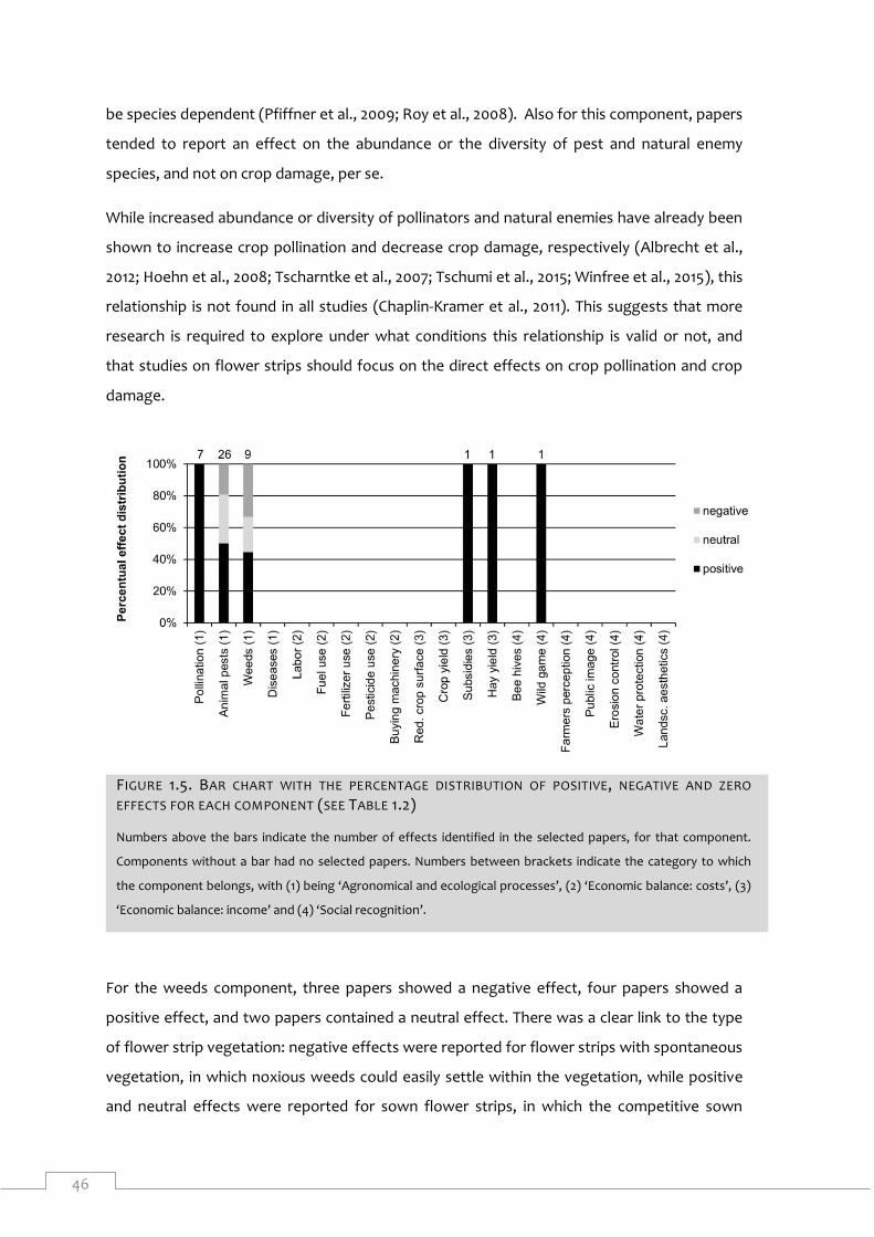
Figure 1.5. Bar chart with the percentage distribution of positive, negative and zero effects

for each component (see Table 1.2) ............................................................................................. 46

Figure 1.6. Plan of the experimental fields in Gembloux ............................................................. 52

Figure 1.7. Picture of a wildflower strip in the ‘Wildflower strips within crop’-field (June 2015)

........................................................................................................................................................ 53

Figure 2.1. Mean expected and realized functional diversity (FD) per treatment ..................... 61

Figure 2.2. Mean total realized number of forb plant species and sown forb plant species for

the different treatments ............................................................................................................... 63

Figure 3.1. Experimental field setup, with Latin square design of sown mixture treatments and

sampling setup per plot with permanent quadrats (PQ) for vegetation monitoring and a

transect for plant-pollinator network sampling .......................................................................... 73

Figure 3.2. a) Realized functional diversity (FD) and b) flower abundance in the different

mixture treatments: very low FD (VL), low FD (L), high FD (H), very high FD (VH), and the

control treatment (Co) .................................................................................................................. 78

Figure 3.3. Wildflower strip plots plotted against the two first ordination axes of Principal

Coordinate Analysis based on the community composition of their flower-visiting insect

community a) in 2014 and b) in 2015 ............................................................................................. 79

Figure 3.4. Bar plots of mean values of the plant-pollinator network metrics for the different

functional diversity (FD) treatments: VL (very low FD), L (low FD), H (high FD), VH (very high

FD) and Co (control mixture) ........................................................................................................ 81

Figure 3.5. Network metric values in function of realized functional diversity (FD) in blue for

2014 and in red for 2015 ................................................................................................................. 84

Figure 3.6. Barplot of significant (P<0.05) Pearson correlations between the Community

Weighted Means of single traits and the network metrics......................................................... 86

Figure 3.7. Barplot of significant (P<0.05) Pearson correlations between the functional trait

diversity of single traits and the network metrics ....................................................................... 87

20

Figure 3.8. Pooled plant-pollinator network for the very low functional diversity mixture in

2014, with plant taxa at the bottom and pollinator taxa at the top. ......................................... 93

Figure 3.9. Pooled plant-pollinator network for the very low functional diversity mixture in

2015, with plant taxa at the bottom and pollinator taxa at the top .......................................... 93

Figure 3.10. Pooled plant-pollinator network for the low functional diversity mixture in 2014,

with plant taxa at the bottom and pollinator taxa at the top .................................................... 94

Figure 3.11. Pooled plant-pollinator network for the low functional diversity mixture in 2015,


Figure 3.12. Pooled plant-pollinator network for the high functional diversity mixture in 2014,


Figure 3.13. Pooled plant-pollinator network for the high functional diversity mixture in 2015,


Figure 3.14. Pooled plant-pollinator network for the very high functional diversity mixture in


Figure 3.15. Pooled plant-pollinator network for the very high functional diversity mixture in


Figure 3.16. Pooled plant-pollinator network for the control mixture in 2014, with plant taxa at

the bottom and pollinator taxa at the top .................................................................................. 97

Figure 3.17. Pooled plant-pollinator network for the control mixture in 2015, with plant taxa at

the bottom and pollinator taxa at the top .................................................................................. 97

Figure 4.1. Stacked bar graph of the mean cover over all quadrats of Cirsium arvense, Rumex

sp. Sinapis alba and the other weeds from June 2014 (J14) to September 2016 (S16) ............. 111

Figure 4.2. Evolution of (a) the mean ln(n+1)-transformed cover of Cirsium arvense and (b)

the mean square root transformed sown forb cover per mowing regime. .............................. 113

Figure 4.3. Mean per seed mixture of (a) the ln(n+1)-transformed cover of Cirsium arvense and

(b) the square root transformed sown forb cover .....................................................................114

Figure 4.4. Plot of the ln(n+1)-transformed cover of Cirsium arvense in September 2016 in

function of (a) the square root transformed sown forb species cover in September 2016 and

(b) the total dry biomass in 2016 ................................................................................................. 116

Figure 4.5. Plan of the experimental field .................................................................................. 119

Figure 5.1. Plant-pollinator networks in the hay meadows......................................................... 131

Figure 5.2. Plant-pollinator networks in the wildflower strips .................................................. 132

Figure 5.3. Principal Coordinate Analysis ordinations of the five wildflower strips (WFS, red

circles) and the five hay meadows (HM, blue circles) ............................................................... 137

21

Figure 6.1. Stacked area chart of the cover of sown forb species in the WM field over three

years ............................................................................................................................................. 145

Figure 6.2. Development of (a) log-transformed flower abundance and (b) flower richness

during the year 2016 in the WM field (Section 1.3) .................................................................... 148

22

23

LIST OF TABLES

Table 1.1. Overview of the components and their respective search terms, questions and

effect definitions for the Scopus query ....................................................................................... 41

Table 1.2. Results of the Scopus query, with for each component the number of papers in the

query output, the number of papers that met the criteria for selection and the references of

these papers .................................................................................................................................. 44

Table 2.1. Species used in the four mixtures ................................................................................ 58

Table 3.1. Plant species used for the four mixtures and their trait values for the selected

functional traits .............................................................................................................................. 71

Table 3.2. Intercept and fixed effects of the selected mixed models for the network metrics

with Likelihood-ratio tests for the predictor variables in the final models ................................ 83

Table 3.3. Mean ± SEM per mixture of the cover of the different plant species found in the

permanent quadrats ..................................................................................................................... 98

Table 3.4. Taxon codes of plant taxa .......................................................................................... 100

Table 3.5. Taxon codes of pollinator taxa ................................................................................... 101

Table 4.1. Species composition of the seed mixtures with the sowing density used per species

...................................................................................................................................................... 107

Table 4.2. Results of F-tests on the fixed effects of the full models ......................................... 112

Table 4.3. Mean and standard error of the cover of sown and spontaneous forb species in

June and September 2016 for the four forb mixtures (F1-F4) and the control mixture (Co) ...120

Table 4.4. Results of the F-tests on the fixed effects of the models fitted for each survey with

Cirsium arvense cover as response variable ................................................................................ 122

Table 4.5. Results of the F-tests on the fixed effects of the models fitted for each mowing

regime with Cirsium arvense cover as response variable ........................................................... 122

Table 4.6. Results of the F-tests on the fixed effects of the models fitted for each survey with

sown forb cover as response variable ......................................................................................... 123

Table 5.1. Pollinator species occurrence in the two habitats ..................................................... 133

Table 5.2. Pollinator species occurrence in the two habitats..................................................... 135

Table 5.3. Mean ± standard error of the different pollinator and plant community responses in

wildflower strips and hay meadows and results of the Student-t test to compare both

habitats ........................................................................................................................................ 138

24

25

CHAPTER 1

INTRODUCTION

26

1. INTRODUCTION

In the introduction chapter, some general concepts upon which this thesis is built are firstly

introduced in the General introduction section. This section is followed by a review paper,

putting flower strips in the socio-economical context of farmers by systematically screening

the literature on existing knowledge. To end this introduction chapter, a last section

describes the objectives and scientific approach of this study.

1.1. GENERAL INTRODUCTION

BIODIVERSITY IN AGROECOSYSTEMS Agriculture in Western Europe and Northern America has known an intensification during last

decades. This intensification mainly consists in scale increase, simplification of crop rotation,

increased pesticide and fertilizer inputs, and creation of drainage and irrigation systems

(Stoate et al., 2001). While intensive agriculture can be an efficient way to produce food,

feed, fiber and fuel, the sustainability of this production system can be questioned. Sources

of fossil fuel for energy input and minerals for fertilizer production are limiting, and the use of

chemical inputs has caused important environmental damage (Cordell et al., 2009; Tilman et

al., 2002).

Furthermore, non-crop habitats in agricultural landscapes decreased in area and got

fragmented. Together with the abovementioned aspects of agricultural intensification, this

has caused biodiversity loss (Kruess and Tscharntke, 1994; Stoate et al., 2001; Tscharntke et

al., 2005). However, farmland biodiversity can deliver important ecosystem services.

Ecosystem services are defined as the benefits people obtain from ecosystems. They include

provisioning services, such as food production, regulating services, such as pollination and

pest control, cultural services, such as recreation and supporting services, such as nutrient

cycling (Millenium Ecosystem Assessment, 2005).

As a response to the increasing demand of food worldwide and the contradiction between

agricultural intensification and ecosystem services by its adverse effects on biodiversity, the

principle of ecological intensification was developed. Ecological intensification tries to

optimize agricultural efficacy by using benefits obtained from ecological processes delivered

by nature (Bommarco et al., 2013). In developed countries, this mainly results in a status quo

of production, while the reliance on chemical and fuel inputs has to be maximally replaced by

27

ecological processes. In developing countries this rather means an increase of the production

by optimizing the ecological processes (Bommarco et al., 2013).

FLOWER STRIPS, THE SUBSIDIZED FIELD BORDERS TO INCREASE BIODIVERSITY Measures for the ecological intensification strategy can be applied at different scales. Inside

the field, the use of compost or manure, crop residue management and reduced tillage

practices are typical examples to improve soil quality and increase soil biodiversity

(Bommarco et al, 2013; Lemtiri et al., 2016; Kovács-Hostyánszki et al., 2017; but see Degrune et

al., 2016). Furtermore, increasing plant diversity within the cropping zone by intercropping, or

using semiochemicals, are within-field methods applied among others for pest management

(e.g. Lopes et al., 2015; Xu et al., 2017). In field edges or borders between fields, hedgerows

and buffer strips can be created to reduce soil erosion, water runoff and nutrient leaching

and to serve as source habitat for ‘functional agrobiodiversity’ (see below) (Tscharntke et al,

2005; Wratten et al, 2012). At the landscape scale, semi-natural habitats can be provided and

networks of ecological infrastructure can connect theses habitats with crop fields

(Tscharntke et al., 2005; Bommarco et al., 2013; Kovács-Hostyánszki et al., 2017). These

FIGURE 1.1. PERENNIAL FLOWER STRIP WITH ADJACENT OILSEED RAPE CROP IN FAIMES, BELGIUM

(MAY 2015)

28

measures are close to the concept of ‘agro-ecological practices’ (Hatt et al., 2016). As for field

edges, an example of a measure, and the focus in this study, is the flower strip.

A flower strip is a part of a field, mostly the field edge, which is covered with herbaceous non-

crop vegetation. This vegetation can develop spontaneously, or a seed mixture can be sown

with the desired species. Seed mixtures can contain grass species, forb species or both.

Flower strips can be annual or perennial (Haaland et al., 2011). In many European countries,

flower strips are part of the subsidized agri-environment schemes of the Common

Agricultural Policy. Farmers adopting such a scheme to reduce the environmental impacts of

their agricultural practices get subsidized to reimburse the yield loss (e.g. by a reduction in

cropping area in case of a flower strip) (European Commission, 2005; Haaland and Gyllin, 2011;

Haaland et al., 2011). The type of strips, management and subsidies vary considerably

between countries, depending on their policy regarding agri-environment schemes (Haaland

et al., 2011). Annual or biennial strips are ploughed and reseeded or translocated every one or

two years respectively. Perennial strips are either left without management, either managed

by mowing to avoid succession. In the former case, the strip has to be ploughed after several

years, because the vegetation becomes dominated by grasses and woody species (Haaland

et al., 2011). In Wallonia (Belgium), perennial strips are usually managed by mowing with a

part of the strip that is left unmown as refuge (Natagriwal asbl, 2017a).

Flower strips mainly aim to enhance farmland biodiversity by providing food and shelter for

insects and other animals, and an area for wild plants to grow and reproduce (Haaland et al.,

2011). On the one hand, they aim to contribute to biodiversity conservation, by increasing

biodiversity or supporting endangered or emblematic species. For this conservation function,

flower strips need to provide one or more of the resources of the species to be supported.

The other resources can be provided by the semi-natural habitats the species in question rely

on, or by the other ecological infrastructure present in the agricultural landscape.

Bumblebees for instance, can use flower strips to provide them with food resources when

flowers are present, while they may rely on flower resources in the surrounding landscape in

early season (Scheper et al., 2015) and on nesting sites in semi-natural habitats (Kells and

Goulson, 2003; Svensson et al., 2000). Scheper et al. (2013) showed that agri-environment

schemes are most effective in an intermediate landscape between cleared (homogeneous

intensive arable landscape, <1% cropped area) and complex (heterogeneous landscape with

arable land and semi-natural habitat, >20% cropped area), which was already suggested by

Tscharntke et al. (2005). In cleared landscape, the very limited source populations are not

29

sufficient to colonize agri-environment schemes. Complex landscapes contain already a high

biodiversity level everywhere, so agri-environment schemes do not have a significant effect.

Furthermore, Kleijn et al. (2011) argue that the efficacy of agri-environment schemes depends

on the ‘ecological contrast’ they deliver, compared to a situation without the scheme.

Indeed, Scheper et al. (2015) showed that flower strips only have an effect on bees when

these strips increase local flower richness. They argue to increase the number of flower

species in flower strips seed mixtures and to use management strategies that maintain this

flower species richness on the long term (Scheper et al., 2015).

The positive effect of flower strips compared to cropped area on insect abundance and

diversity has been extensively shown (reviewed by Haaland et al., 2011). However, few

studies verified if flower strips really serve as a surrogate habitat for insect communities or

rather as new habitat with another associated insect community. Indeed, flower strips are, in

contrast to other agri-environment schemes, considered as a rather new habitat in the

agricultural landscape, making it difficult to define guidelines for their creation and

management. In countries where grasses are added to the mixtures of perennial flower

strips, and strips are managed by mowing, they can be compared to hay meadows (Haaland

et al., 2011). Öckinger and Smith (2007) showed in a Swedish experiment that the original

semi-natural habitat (grassland) functions as a source population for the species to colonize

the surrogate habitat (uncultivated field margins). Similarly, Ekroos et al. (2013) found that

abundance and diversity of bumblebees and butterflies, but not syprhid flies, was lower in

linear habitat elements more distant from semi-natural grassland. However, Haaland and

Bersier (2011) found in their study in Switzerland that the butterfly species community in

perennial flower strips was not a subset of the butterfly community in extensive meadows.

More research is needed to identify the role of agri-environment schemes in comparison to

the semi-natural habitat for which they are thought to be a surrogate.

On the other hand, the aim of flower strips is to attract and support useful arthropods, also

called ‘functional agrobiodiversity’ (Bianchi et al., 2013), like pollinators (Nicholls and Altieri,

2012) and natural enemies of crop pests (Landis et al., 2000). Flower strips have been shown

to increase pollination services to crops by supporting pollinators (Barbir et al., 2015; Blaauw

and Isaacs, 2014; Feltham et al., 2015), while some studies found no effect (e.g. Campbell et

al., 2017). To attract these arthropods, recent studies propose to develop tailored flower

strips to maximize the regulating services delivered by flower strips to the crop (e.g. Tschumi

et al., 2014, 2016). For this kind of strips, a specific set of plant species is selected that is

30

known to attract the specific set of functional arthropods for the crop in the adjacent field

(Tschumi et al., 2014). This results however in annual or biennial flower strips that are

included in a crop rotation and for which the longer term conservation value can be

questioned. Perennial flower strips in contrary, could host a permanent community of plants

and associated fauna that can deliver multiple and stable ecosystem services on a longer

term. Tscharntke et al. (2005) argue to focus on a diversity of species and processes in land-

use management to increase resilience of the system. Next to pollination and pest control

services, flower strips are also expected to deliver other ecosystem services. They can limit

soil erosion, nutrient leaching and surface water runoff, and improve nutrient cycling.

Furthermore, flower strips can help suppressing weeds, and improve rural prosperity and

landscape aesthetics (Wratten et al., 2012).

FUNCTIONAL DIVERSITY, THE KEY COMPONENT OF BIODIVERSITY? Increasing biodiversity has been shown to be a strategy to optimize ecosystem functioning

and ecosystem services (Díaz et al., 2005). Increasing plant diversity could thus be a goal for

the creation and management of flower strips, as suggested by Scheper et al. (2015).

However, in the relationship between biodiversity and ecosystem functioning and ecosystem

services, not species per se, but their functional traits have been suggested to play a key role

(Dı́az and Cabido, 2001). Functional traits are defined as “morphological, biochemical,

physiological, structural, phenological, or behavioral characteristics that are expressed in

phenotypes of individual organisms and are considered relevant to the response of such

organisms to the environment and/or their effects on ecosystem properties” (Díaz et al.,

2013). Not the species, but their functional traits define their response to the environment

and to other species and their effect on other organisms and on ecosystem processes. For

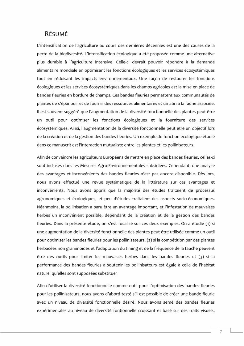
illustration, the example of the study of Fontaine et al. (2006) is given here. They studied the

interaction of pollinators and plants in a cage experiment. Two plant types were defined

regarding corolla depth: open flowers and tubular flowers (see Figure 1.2). The corolla depth

FIGURE 1.2. EXAMPLE OF A CAGE EXPERIMENT WITH POLLINATOR AND PLANT SPECIES GROUPED FOR

THEIR FUNCTIONAL TRAITS 'MOUTHPART LENGTH' AND 'COROLLA DEPTH' (FONTAINE ET AL., 2006)

31

can be considered as a functional effect trait in this experiment (Díaz et al., 2013; Lavorel et

al., 2013), as it defines whether floral rewards (pollen and nectar) are easily accessible or not

for pollinators (Figure 1.2). Secondly, two pollinator types were defined regarding their

mouthparts length: syrphid flies (Diptera: Syrphidae) with short mouthparts and bumblebees

(Hymenoptera: Apidae) with long mouthparts. Mouthparts length can be considered as a

functional response trait in this experiment, as it defines whether the pollinator can access

floral rewards in a flower (Díaz et al., 2013; Lavorel et al., 2013). Syrphid flies with short

mouthparts are not expected to pollinate tubular flowers, while bumblebees with long

mouthparts are expected to pollinate both types of flowers (Figure 1.2). As these traits

determine the access to floral rewards, the presence or absence of plant and pollinator

species with the different levels for the traits can influence the reproductive success of plants

(Fontaine et al., 2006). When applying this approach to flower strips, sowing strips containing

plant species with different levels for the trait ‘corolla depth’ can attract a higher diversity of

flower-visiting insects than sowing strips containing only one level (Campbell et al., 2012;

Wratten et al., 2012). The number of levels of a functional trait is also called the ‘functional

group richness’ and signifies the number of functional groups represented. It is an example

of a metric of functional diversity (FD), which is the value and range of functional traits

(Tilman, 2001). This FD is not to be confounded with functional agrobiodiversity (see above),

i.e. biodiversity that provides ecosystem services for sustainable agricultural production

(Bianchi et al., 2013). Functional group richness appears to be the most commonly used

metric of FD in community ecology studies (Mason et al., 2005), as it is easy and quick to

group species that are similar in their functional traits.

More precise indices of FD try to measure it on a continuous scale and are related to the

ecological niches of the species present. Three groups of indices can be distinguished (Mason

et al., 2005; Schleuter et al., 2010): Functional richness indices (the trait value range or niche

range occupied by the species community), functional evenness indices (the degree of equal

distribution of the trait values occupied in the trait value range), and functional divergence

indices (the degree of niche differentiation, or the degree of clustering of species or

abundances at the edges of trait values range). Depending on the index, one or several traits

can be used to calculate the index (Schleuter et al., 2010). A FD metric that was used in this

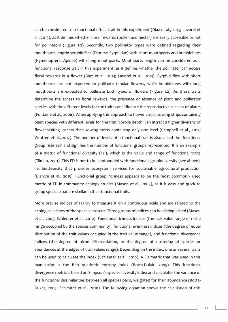
manuscript is the Rao quadratic entropy index (Botta-Dukát, 2005). This functional

divergence metric is based on Simpson’s species diversity index and calculates the variance of

the functional dissimilarities between all species pairs, weighted for their abundance (Botta-

Dukát, 2005; Schleuter et al., 2010). The following equation shows the calculation of this

32

index (for S species, with dij the distance between species i and species j based on their

functional traits, and pi and pj the relative abundances of species i and j):

𝐹𝐷𝑅𝑎𝑜 =∑ ∑ 𝑑𝑖𝑗𝑝𝑖𝑝𝑗

𝑆

𝑗=𝑖+1

𝑆−1

𝑖=1

The advantage of this metric is that it takes into account the relative abundance of different

species and thus of their trait values, unlike functional richness metrics. Furthermore, it is not

correlated with species richness and it is the only functional divergence metric that can both

take into account multiple traits and categorical traits (Schleuter et al., 2010).

As functional traits may play a key role in the biodiversity-ecosystem functioning relationship,

it is often suggested that biodiversity should be approached as FD, which is thought to be a

better predictor than species diversity in this relationship (Dı́az and Cabido, 2001). Therefore,

increasing plant functional diversity instead of plant species diversity can be a tool to

optimize ecosystem functioning and ecosystem service delivery in flower strips. However,

few evidence exists on this relationship, especially in the context of flower strips.

ECOSYSTEM FUNCTIONING: THE CASE OF PLANT-POLLINATOR NETWORKS An example of ecosystem functioning studied in this manuscript, is the mutualistic interaction

between plants and pollinators. Wild pollinators are among the functional groups that

suffered declines due to land use intensification (Biesmeijer et al., 2006; Potts et al., 2010;

Winfree et al., 2009). In the IPBES “Assessment report on pollinators, pollination and food

production”, ecological intensification, strengthening existing diverse farming systems and

investing in ecological infrastructure were identified as complementary methods to both

maintain healthy pollinator communities and productive agriculture (IPBES, 2016). Pollinators

visit plant flowers to obtain floral rewards like nectar and pollen. By visiting different flowers

and transporting pollen between flowers, they contribute to the pollination of these plants.

As such, animal pollinators play an important role in the pollination of wild plants and crops

worldwide (Klein et al., 2007; Potts et al., 2010). For wild plants, 60 to 80% of the species

depend on animal pollinators (Kremen et al., 2007). As for crops, Klein et al. (2007) calculated

that the production of 70% of the most important crops worldwide is increased with animal

pollination. In terms of production mass, only 36% of the produced crop mass is increased

with animal pollination, as the crops with the highest production are wind-pollinated or

passively self-pollinated. Moreover, while some animal-pollinated crops need pollination to

produce fruits that are consumed, other crops are produced for the consumption of

33

vegetative parts and pollination is only needed for reproduction or breeding (Klein et al.,

2007). For Belgium, it was calculated that 11.1% of the crop production value in 2010, or 251.62

million €, was dependent on pollinators. 82% of this amount was attributed to fruits

production, 18% to vegetables and less than 1% to oil crops and legumes (Jacquemin et al.,

2017). Furthermore, as the crop pollination service is mainly delivered by a set of common

pollinator species, this ecosystem service may not be a sufficient argument for the

conservation of pollinator diversity including rare species (Kleijn et al., 2015).

Studying the complex network of interactions between plant species and pollinator species

delivers interesting information on the structure, stability and intensity of this ecosystem

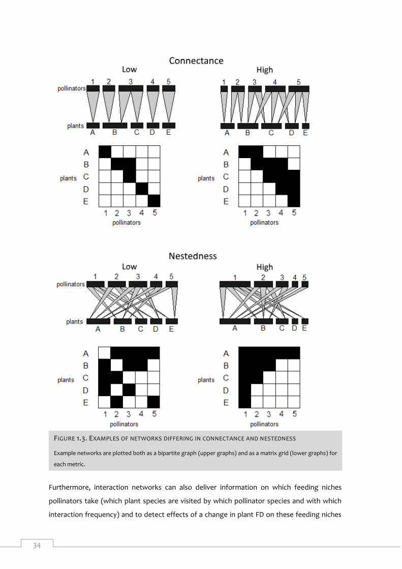
functioning (Tylianakis et al., 2010). Some examples of interaction networks are given in

Figure 1.3. These networks are constructed by observing which pollinator species visit which

plant species (‘links’) and how frequently these visits occur (‘interactions’). A metric that is

often calculated for plant-pollinator networks is ‘network connectance’ (Figure 1.3). This is

the ratio between the number of realized links and the number of possible links of the

network (Tylianakis et al., 2010). In Figure 1.3 for instance, the highly connected network has

got 11 out of 25 possible links that are realized, while the lowly connected network only 6. A

higher network connectance is associated with a higher rate of ecosystem processes and a

higher ecosystem process stability (Thébault and Fontaine, 2010; Tylianakis et al., 2010).

Another metric is network nestedness (Figure 1.3). In a nested network, species interacting

with specialists are a proper subset of species interacting with generalists. As specialists have

higher chance to go extinct, in a nested network their interaction partners are secured by

also interacting with generalist species (Thébault and Fontaine, 2010; Tylianakis et al., 2010).

In the highly nested network in Figure 1.3 for instance, if the specialist plant species D (it only

interacts with pollinator species 1) goes extinct, pollinator species 1 is well secured from

secondary extinction as it interacts with generalist plant species A and B.

34

Furthermore, interaction networks can also deliver information on which feeding niches

pollinators take (which plant species are visited by which pollinator species and with which

interaction frequency) and to detect effects of a change in plant FD on these feeding niches

FIGURE 1.3. EXAMPLES OF NETWORKS DIFFERING IN CONNECTANCE AND NESTEDNESS

Example networks are plotted both as a bipartite graph (upper graphs) and as a matrix grid (lower graphs) for

each metric.

35

(Junker et al., 2013). Indeed, changing the niches available by changing the plant FD can be

expected to affect the composition of pollinator species that are able to find their required

feeding niche and the complementarity or redundancy of these pollinator species in their

feeding niche. When increasing plant species richness per se, each additional species can

bring either complementary or redundant trait values to the trait value composition of the

plant species community. Redundant species can play the role of ‘insurance species’ and take

the functions of other species with the same functions in case of the loss of these species due

to disturbance (Dı́az and Cabido, 2001). While some argue that only few abundant key species

deliver the important ecosystem services (Kleijn et al., 2015; Winfree et al., 2015), this

insurance effect of redundant species might be important to take into account in the

development of sustainable agri-environment schemes (Tscharntke et al., 2005).

36

1.2. PROS AND CONS OF FLOWER STRIPS FOR FARMERS. A REVIEW

Review paper published in Biotechnology, Agronomy, Society and Environment (2016),

20(S1):225-235

ROEL UYTTENBROECK, SÉVERIN HATT, AMAN PAUL, FANNY BOERAEVE, JULIEN PIQUERAY, FRÉDÉRIC

FRANCIS, SABINE DANTHINE, MICHEL FRÉDÉRICH, MARC DUFRÊNE, BERNARD BODSON, ARNAUD MONTY

ABSTRACT Description of the subject. To counteract environmental problems due to agricultural

intensification, European farmers can apply agri-environmental schemes in their fields.

Flower strips are one example of these schemes, with the aim of supporting biodiversity,

leading to an increase in ‘useful’ species groups such as pollinators for crop pollination and

natural enemies for pest control. However, to our knowledge, a complete appraisal of the

pros and cons of flower strips, from a farmer’s point of view, does not yet exist. It is

proposed that better and more complete information could increase the adoption and

implementation of such agri-environmental schemes.

Objectives. This study aims 1) to assess the pros and cons of flower strips, from a farmer’s

point of view, and 2) to highlight the knowledge gaps that exist in the scientific literature, for

the different types of pros and cons.

Method. We listed the different components of the appraisal of pros and cons and conducted

a systematic screening of the scientific literature on flower strips and these components.

Results. The largest part of the 31 selected studies was concerning agronomical and

ecological processes, such as pollination and animal pest control. Most of them indicated

positive effects of flower strips. For many components of the appraisal, mostly economic and

social ones, few or no studies were found.

Conclusions. While a positive balance of pros and cons, from a farmer’s point of view, came

from our literature screening, large research gaps still remain and more research is required,

especially in the economic and social components of the evaluation.

Key words

Agroecosystems, ecosystem services, sustainable agriculture, agricultural practices, intensive

farming, crop yield, compensation, farm income, attitudes, biological control

37

INTRODUCTION Agricultural intensification during the last few decades has led to large biodiversity losses,

due to habitat destruction and fragmentation, increased field size, simplified crop rotations

and intensification of crop management (Kruess and Tscharntke, 1994; Stoate et al., 2001;

Tscharntke et al., 2005). Simultaneously, the concept of Ecosystem Services (ES) arose,

defined as the benefits that people obtain from ecosystems (Millenium Ecosystem

Assessment, 2005). In the field of agriculture, ES are, among others, biomass production,

pollination, pest control, soil conservation and fertility (Zhang et al., 2007). As biodiversity is

known to play a key role in ES, biodiversity losses can cause disruption of ES delivered by the

agricultural landscape (Tscharntke et al., 2005; Zhang et al., 2007). Increasing and restoring

biodiversity in the agricultural landscape can, thus, be a strategy to support these ES.

Therefore, European farmers are encouraged through European subsidies of the Common

Agricultural Policy to implement agri-environmental schemes, such as planting hedgerows,

grass buffer strips or flower strips (European Commission, 2005; Haaland et al., 2011). A

flower strip is a part of a field that is preserved for herbaceous vegetation. The strip can be

created by sowing a mixture of forb species, with or without grass species. The strip can also

be created by spontaneous vegetation. Both annual and perennial strips exist. The type of

strips, management and subsidies vary considerably between countries, depending on their

policy (Haaland et al., 2011). The main goal of flower strips is to enhance farmland biodiversity

by providing food and shelter for insects and other animals, and an area for wild plants to

grow and reproduce (Haaland et al., 2011). Additionally, their focus is to attract and support

functional arthropods like pollinators (Nicholls and Altieri, 2012) and natural enemies (Landis

et al., 2000). These functional arthropods can be beneficial to the crop by delivering

pollination and pest control services and can reduce inputs like pesticide use or renting bee

hives (Haaland et al., 2011), making flower strips a valuable measure to play a role in

ecological intensification (Bommarco et al., 2013). Apart from supporting and attracting

functional arthropods, habitat enhancement, like the implementation of flower strips, can

also provide other advantages, such as reduction of soil erosion or improvement of the

landscape’s aesthetic value (Fiedler et al., 2008; Wratten et al., 2012).

While some of these advantages have already been shown, agri-environmental schemes have

been discussed over the years, as they are not always effective (Batáry et al., 2015). Reviews

exist on sown flower strips (Haaland et al., 2011) or field margins (Marshall and Moonen,

2002), but they are restricted to the effect of sown flower strips on insect conservation

(Haaland et al., 2011) and interactions of field margins with agriculture (Marshall and Moonen,

38

2002) and do not provide a complete appraisal of the advantages and disadvantages of

flower strips. Some attempts have been made to evaluate the pros and cons of habitat

enhancement, such as in Fiedler et al., (2008) and Wratten et al. (2012), but not yet for flower

strips specifically. Bommarco et al. (2013) argue that existing knowledge gaps on several

services and processes, as well as on their synergies and trade-offs, have implications for

decision making in ecological intensification measures. Moreover, many studies about the

farmers’ attitude towards the adoption of agri-environmental schemes demonstrate the

importance of providing information on the diverse aspects of their implementation (Burton

and Paragahawewa, 2011; Mante and Gerowitt, 2007; Mathijs, 2003; Sattler and Nagel, 2010;

Vanslembrouck et al., 2002). Apart from environmental concern, compensation rates and the

effect on agronomic production, the farmers’ acceptance of agri-environmental schemes is

also driven by implementation time and effort, effectiveness, associated risks, additional

transaction costs, their ease in communication and their relations with the subsidizing

institution and its contact person (Falconer, 2000; Mante and Gerowitt, 2007; Mathijs, 2003;

Sattler and Nagel, 2010). It was shown that farmers who are more informed and more

convinced about the usefulness of agri-environmental schemes, are more likely to implement

them in their farms (Vanslembrouck et al., 2002). Moreover, Burton and Paragahawewa

(2011) argue that this information would increase the adoption of environmental practices in

their farming culture and conventional ‘good farming’ practice. Therefore, it could be useful

to gain comprehensive insight into the advantages and disadvantages of the implementation

of flower strips for farmers (Fiedler et al., 2008; Wratten et al., 2012). In this context, we

conducted a systematic literature screening aiming at 1) assessing the pros and cons from a

farmer’s point of view, and 2) highlighting the knowledge gaps in the literature for the

different types of pros and cons.

LITERATURE SCREENING To make an appraisal of the pros and cons of flower strips, a list was made of the possible

different components of this appraisal, that is, aspects of the farming system that may be

influenced by a flower strip. This list of components was iteratively composed and completed

by a panel of experts. This panel was comprised of the authors of this manuscript, being

researchers and professors with a MSc or PhD degree and having expertise in crop science,

ecology, weed science, ecosystem service valuation, agroecology, food science, pollination

and biological control. The components can be found in Table 1.1. They were divided into four

categories: i) Agronomical and ecological processes: the effect on the crop of ecosystem

processes in the flower strip; ii) Economic balance (costs): the different economic inputs that

39

can be influenced by flower strips; iii) Economic balance (income): the different economic

outputs that can be influenced by flower strips; iv) Social recognition: the different ways that

a farmer’s relationship with other stakeholders can be influenced by flower strips, and the

farmer’s perception of flower strips.

For each component, a search query was done in Scopus (Elsevier B.V., 2014) scientific

literature database on 31 October 2014. For this, keywords were chosen to find literature

addressing flower strips and the respective component. The query syntax required the

papers to have title, abstract or keywords containing at least one of the search terms about

flower strips and at least one of the search terms about the respective component. The

search terms about flower strips were ‘flower strip(s)’, ‘wildflower strip(s)’, ‘flowering

border(s)’, ‘flower margin(s)’, ‘margin strip(s)’, ‘sown strip(s)’, ‘sown margin(s)’, ‘sown

margin strip(s)’, ‘weed strip(s)’, ‘sown weed strip(s)’, ‘herb strip(s)’, ‘sown herb strip(s)’,

‘field margin(s) AND sowing’, ‘field boundary/boundaries AND sowing’ and ‘field border(s)

AND sowing’. The search terms for the components are listed in Table 1.1. Search terms were

chosen to find as many papers as possible that were clearly about flower strips and the

respective component. For this, the list of search terms was again subject to validation by the

panel of experts.

To retain only the papers that met the objectives of this review, the references obtained from

the Scopus search query were listed, per component, and divided between the authors to

select the references of interest based on a set of criteria (see below). If an abstract was not

available, the reference was not considered. Review papers were not considered, as these

are based on other studies. Double records, or studies published more than once, were only

considered once.

To be selected, a paper had to meet four criteria. Firstly, the study had to be about flower

strips, a part of a field that contained one or more forb (herbaceous flowering) species. This

part could be at the margin or inside the field, the vegetation could be spontaneous or sown,

the plant species could be native or not, and annual or perennial. Excluded were pure grass

strips, hedgerows (strips of ligneous plants), crop associations and companion plants.

Included were strips where a crop and annual forbs were mixed. The decision for this

criterion was made based on the abstract, but if the detailed characteristics of the flower

strip could not be derived from the abstract, they were verified in the body of the article.

Secondly, the study had to be conducted in an agricultural context. This means that the part

of the field, that is not flower strip, had to be cropland, pasture or orchard. It also means the

40

study had to be conducted in the field, not in controlled conditions (lab, greenhouse, growth

chamber, etc.). The decision was taken based on the abstract, but if the agricultural context

was not clear from the abstract, it was verified in the body of the article. Thirdly, the study

had to be about the respective component of the appraisal. For this, a clear question was

formulated for each component to evaluate the abstracts. The questions are listed in Table

1.1. This criterion had to be clear from the abstract. As the presence of a healthy pollinator

community and a healthy natural enemy community are considered to be beneficial for crop

pollination and crop pest control, respectively (e.g. Albrecht et al., 2012; Chaplin-Kramer et al.,

2011; Hoehn et al., 2008; Tscharntke et al., 2007; Tschumi et al., 2015; Winfree et al., 2015),

they were also used in the third criterion for the components ‘pollination’ and ‘animal pests’.

For this third criterion, the selection procedure was cross-checked by providing the set of

references, meeting each criterion, to another author to evaluate them again, with the third

criterion. Fourthly, the study had to be conducted in the North Temperate Zone (between

the Arctic Circle and the Tropic of Cancer). If this was not clear from the abstract, it could be

verified in the body of the article.

41

TABLE 1.1. OVERVIEW OF THE COMPONENTS AND THEIR RESPECTIVE SEARCH TERMS, QUESTIONS AND EFFECT DEFINITIONS FOR THE SCOPUS QUERY

Components Search terms

Question: Does the paper investigate…

Positive effect: Flower strips result in…

Neutral effect: No effect of flower strips is found on…

Negative effect: Flower strips result in…

Ag

ron

om

ical

an

d e

colo

gic

al p

roce

sse

s

Pollination pollination, pollinator(s) whether flower strips have an impact on crop pollination or on a healthy pollinator community (abundance, diversity,…)?

better or more crop pollination or in a healthier pollinator community (abundance, diversity,…)

crop pollination or on the health of the pollinator community (abundance, diversity,…)

worse or less crop pollination or in a less healthy pollinator community (abundance, diversity,…)

Animal pests insects pests, animal pests, slugs, rodents, pest management, pest control, natural enemies, predators, predation, parasitism, parasitoids, herbivory, herbivores

whether flower strips have an impact on animal pests on crops or whether it affects the natural enemy community (abundance, diversity)?

fewer animal pests on crops or in a healthier natural enemy community (higher abundance, diversity)

animal pests on crops or on the natural enemy community (abundance, diversity)

more animal pests on crops or in a less healthy natural enemy community (lower abundance, diversity)

Weeds weed, weeds whether flower strips have an impact on weeds (spreading) in the cropping area?

less weeds (spreading) in the cropping area

weeds (spreading) in the cropping area

more weeds (spreading) in the cropping area

Diseases diseases, fungi, pathogens, infection, virus, bacteria, plant pathology, phytopathology, immunology, epidemiology

whether flower strips have an impact on crop diseases?

less crop diseases crop diseases more crop diseases

Eco

no

mic

bal

ance

: co

sts

Labor labor, human labor, labour, human labour

whether flower strips have an impact on the farmer's labor?

a decrease in farmer’s labor

on the farmer’s labor an increase of farmer’s labor

Fuel use fuel, energy whether flower strips have an impact on the farmer's fuel use?

a decrease of the farmer's fuel use

the farmer's fuel use an increase of the farmer's fuel use

Fertilizer use fertilizers, fertilizer, manure whether flower strips have an impact on the fertilizer use in the crop field?

less fertilizer use in the crop field

on fertilizer use in the crop field

greater fertilizer use in the crop field

Pesticide use pesticides, crop protection, herbicide, insecticide, biocide, fungicide, molluscicide

whether flower strips have an impact on the pesticide use in the crop field?

less pesticide use in the crop field

on pesticide use in the crop field

greater pesticide use in the crop field

Buying machinery

equipment, machine, mowing, cutting

whether flower strips have an impact on the equipment the farmer has to buy/rent/own?

a decrease in the equipment the farmer has to buy/rent/own

on the equipment the farmer has to buy/rent/own

an increase in the equipment the farmer has to buy/rent/own

42

Components Search terms

Question: Does the paper investigate…

Positive effect: Flower strips result in…

Neutral effect: No effect of flower strips is found on…

Negative effect: Flower strips result in…

Eco

no

mic

bal

ance

: in

com

e

Reduction in crop surface area

crop surface, crop area, cultivated surface, cultivated area

whether flower strips have an impact on the surface on which cropping can be done?

a greater surface area on which cropping can be performed

the surface on which cropping can be performed

a reduced surface on which cropping can be performed

Crop yield Yield whether flower strips have an impact on the crop yield?

a higher crop yield the crop yield lower crop yield

Subsidies subsidies, reward, refunding, politics, incentive, policy, compensation

whether flower strips have an impact on the farmer's subsidies?

more subsidies for the farmer

the farmer's subsidies less subsidies for the farmer

Hay yield hay, forage, herbage, grazing, fibre, protein, biofuel, bioenergy, bioethanol

whether flower strips have an impact on the hay yield produced in the field (by the flower strip), or whether this hay is a profitable product?

more hay yield produced in the field (by the flower strip); or the produced hay to be a profitable product

the hay yield produced in the field (by the flower strip); or there is no net profitability of the hay as product

a lower hay yield produced in the field (by the flower strip); or the produced hay to be an unprofitable product

So

cial

re

cog

nit

ion

Bee hives hive, Apis mellifera, honey bee, beekeeping, honey

whether flower strips have an impact on the number of bee hives that can be put in the field, or on the honey production?

more bee hives that can be put in the field or more honey production

the amount of bee hives that can be put in the field or on the honey production

less bee hives that can be put in the field or less honey production

Wild game wild game, hunting, hunters whether flower strips have an impact on the wild game in the landscape?

more wild game in the landscape

the wild game in the landscape

less wild game in the landscape

Farmer’s perception

farmer perception, farmer acceptance

the farmer's perception/acceptance of flower strips?

a positive perception of flower strips by farmers

farmer’s perception of flower strips

a negative perception of flower strips by farmers

Public image farmer, image, esteem whether flower strips have an impact on the image society has of a farmer?

a better image of a farmer held by society

the image of a farmer held by society

a worse image of a farmer held by society

Erosion control

erosion, runoff, soil loss whether flower strips have an impact on the soil loss from the field?

a decrease of the soil loss from the field

the soil loss from the field an increase of the soil loss from the field

Water protection

leaching, water protection, water quality, ground water, surface water

whether flower strips have an impact on the water quality or water pollution?

an improvement of water quality or less water pollution

the water quality or water pollution

lower water quality or more water pollution

Landscape aesthetics

Landscape, tourism, ecotourism, aesthetic, recreation

whether flower strips have an impact on the landscape aesthetics, tourism or recreation?

better landscape aesthetics, more tourism, or more recreation

the landscape aesthetics, tourism or recreation

worse landscape aesthetics, less tourism, or less recreation

TABLE 1.1 (CONTINUED). OVERVIEW OF THE COMPONENTS AND THEIR RESPECTIVE SEARCH TERMS, QUESTIONS AND EFFECT DEFINITIONS FOR THE SCOPUS QUERY

43

Based on the number of selected papers per component, the knowledge gaps and research

needs were highlighted. The selected papers were then screened for the type of effect they

showed. We considered as an effect a relationship, found in a study, showing an influence of

flower strips on the considered component: a ‘positive effect’ if the study showed that

flower strips had a significant influence on the component that was beneficial for the farmer;

a ‘negative effect’ if the study showed that flower strips had a significant influence on the

component that was disadvantageous for the farmer; and a ‘neutral effect’ if the study

contained a relationship for which no significant influence on the component could be shown

(see Table 1.1 for a clear definition of the effects per component). A single paper could show

positive, neutral, as well as negative effects, which, in that case, were all considered. If a

paper showed an effect for which no statistical test was needed, it was also taken into

consideration. The information on the effects was based on the abstract, but if the

information could not be derived from the abstract, it was verified in the body of the article.

The effects were summed, per component, to identify the predominant effect.

FLOWER STRIPS’ PROS AND CONS FOR FARMERS: A POSITIVE BALANCE SO FAR The Scopus search retrieved 245 unique records, among which some appeared for several

components, resulting in a total of 593 records. Only 34 records met the criteria for selection,

of which 30 were unique papers. The selected papers addressed 6 of the 20 components (see

Table 1.2): pollination, animal pests, weeds, subsidies, hay yield and wild game. Most selected

papers addressed the animal pests component (18), followed by pollination (7) and weeds

(6). Figure 1.4 shows a radar plot of the log-transformed (log [n+1]) number of selected

papers, for each component. Most selected papers (31 out of 34) appeared in the

‘agronomical and ecological processes’ category, while the components of the other

categories had only one selected paper, or none at all.

Figure 1.5 shows the percentage of positive, negative and neutral effects (from a farmer’s

point of view) of the selected papers, for each component. In total, 80% of the papers

reported positive effects, 24% reported negative effects and 29% reported neutral effects.

This resulted in 27 positive effects reported, 10 negative effects and 8 neutral effects. As

explained before, a single paper could contain a positive, a negative, as well as a neutral

effect. There was not a single case among the components where the negative effects

outweighed the positive effects. While this already suggests a positive balance of pros and

cons, the lack of research for most of components makes it too early to draw any general

conclusions.

44

Components Number of papers output

Number of selected papers

References selected papers

Pollination 23

7 Balzan et al., 2014+; Carvell et al., 2011+; Heard et

al., 2007+; Korpela et al., 2013+; Potts et al., 2009+;

Pywell et al., 2011+; Rundlöf et al., 2014+

Animal pests 95 18 Anjum-Zubair et al., 2010+,0; Balzan et al., 2014+,-

Bigger and Chaney, 19980; Büchi, 20020; Denys and Tscharntke, 2002+; Eyre et al., 20110; Fitzgerald and Solomon, 20040; Hausammann, 1996+; Hickman and Wratten, 1996+,0; Meek et al., 2002+,0; Pascual-Villalobos et al., 2006-; Pfiffner and Luka, 2000+; Pfiffner et al., 2009+,0; Pywell et al., 2011+,-; Roy et al., 2008+; Skirvin et al., 2011+; Walton and Isaacs, 2011+,-; Wyss, 1996+,0

Weeds 71 6 Bokenstrand et al., 2004+,0; De Cauwer et al., 2008+,-; Denys and Tscharntke, 2002+,-; Marshall, 2001+; Moonen and Pywell et al., 2011-; Smith et al., 19990

Diseases 15 0

Labor 0 0

Fuel use 7 0

Fertilizer use 30 0

Pesticide use 73 0

Buying machinery 46 0

Reduction crop surface area 41 0

Crop yield 35 0

Subsidies 58 1 Mante and Gerowitt, 2007+

Hay yield 38 1 De Cauwer et al., 2006+

Bee hives 8 0

Wild game 13 1 Casas and Viñuela, 2010+

Farmers perception 0 0

Public image 24 0

Erosion control 8 0

Water protection 5 0

Landscape aesthetics 3 0

TABLE 1.2. RESULTS OF THE SCOPUS QUERY, WITH FOR EACH COMPONENT THE NUMBER OF PAPERS IN THE

QUERY OUTPUT, THE NUMBER OF PAPERS THAT MET THE CRITERIA FOR SELECTION AND THE REFERENCES OF

THESE PAPERS

‘+’: the paper shows a positive effect; ‘-‘: the paper shows a negative effect; ‘0’: the paper shows a neutral effect

45

For the pollination component, all seven selected papers showed a positive effect, being an

increase in either abundance or diversity of pollinators, or both. Haaland et al. (2011) and

Marshall and Moonen (2002) already mentioned some work suggesting the beneficial effect

of flower strips for pollinators in their reviews. Five out of these papers considered

bumblebees as the taxonomic group to study pollination. No paper was found investigating

the effect on crop pollination explicitly.

For the animal pests component, 13 papers showed a positive effect, 5 papers showed a

negative effect, and 8 papers contained a neutral effect. Effects concerned either an increase

or decrease in abundance or diversity of pests, either an increase or decrease in abundance

or diversity of natural enemies, or both. The positive effects, consisting in the reduction of

pests or the increase of natural enemies, have also been mentioned in the review of Marshall

and Moonen (2002) while the reviewed papers in Haaland et al. (2011) also showed mixed

effects (reviewed papers partly overlapping with the papers in the present review). While

abundance was the most frequently used metric, four papers also studied diversity, or

species richness, of pests or natural enemies. Some of the papers indicated that effects can

FIGURE 1.4. RADAR PLOT OF THE LOG-TRANSFORMED (LOG (N+1)) NUMBER OF PAPERS SELECTED FOR

EACH COMPONENT

Numbers between brackets indicate the category to which the component belongs, with (1) being ‘Agronomical

and ecological processes’, (2) ‘Economic balance: costs’, (3) ‘Economic balance: income’ and (4) ‘Social

recognition’.

46

be species dependent (Pfiffner et al., 2009; Roy et al., 2008). Also for this component, papers

tended to report an effect on the abundance or the diversity of pest and natural enemy

species, and not on crop damage, per se.

While increased abundance or diversity of pollinators and natural enemies have already been

shown to increase crop pollination and decrease crop damage, respectively (Albrecht et al.,

2012; Hoehn et al., 2008; Tscharntke et al., 2007; Tschumi et al., 2015; Winfree et al., 2015), this

relationship is not found in all studies (Chaplin-Kramer et al., 2011). This suggests that more

research is required to explore under what conditions this relationship is valid or not, and

that studies on flower strips should focus on the direct effects on crop pollination and crop

damage.

For the weeds component, three papers showed a negative effect, four papers showed a

positive effect, and two papers contained a neutral effect. There was a clear link to the type

of flower strip vegetation: negative effects were reported for flower strips with spontaneous

vegetation, in which noxious weeds could easily settle within the vegetation, while positive

and neutral effects were reported for sown flower strips, in which the competitive sown

FIGURE 1.5. BAR CHART WITH THE PERCENTAGE DISTRIBUTION OF POSITIVE, NEGATIVE AND ZERO

EFFECTS FOR EACH COMPONENT (SEE TABLE 1.2)

Numbers above the bars indicate the number of effects identified in the selected papers, for that component.

Components without a bar had no selected papers. Numbers between brackets indicate the category to which

the component belongs, with (1) being ‘Agronomical and ecological processes’, (2) ‘Economic balance: costs’, (3)

‘Economic balance: income’ and (4) ‘Social recognition’.

47

species were able to suppress harmful weed species from settling in the strip. Marshall and

Moonen (2002) also mention research pointing out that sowing grass, or grass and flower

mixes, reduces the risk of weed spreading.

For the subsidies, the hay yield as well as the wild game component, only one paper was

selected, each one showing a positive effect of flower strips. For the other components,

either no papers were found or the papers did not meet the criteria. The small number of

selected papers, therefore, makes it impossible to draw general conclusions. However, for

certain components, the effects of flower strips might be obvious. For example, flower strips

can produce hay, while crops mostly don’t. Hay yield is, thus, expected not to be negatively

affected by implementing flower strips instead of crops.

RESEARCH GAPS AND NEED FOR FURTHER RESEARCH While a total of 593 records came out of the database query, only 34 met the criteria for

inclusion. This shows that, from the considerable amount of research on flower strips, only a

few studies explicitly considered the influence of flower strips in terms of the advantages or

disadvantages for the farmer. For pollination, animal pests, and weeds, many papers had to

be excluded as they reported on insects or weeds in the crop or flower strip, without a

proper comparison to a no-strip control. This partly explains the low number of selected

papers for these components, and suggests the need for well-designed field studies to

demonstrate the effects of flower strips. Moreover, only one study was carried out over 10

years, while the other studies lasted only for four years or less. More long-term research

could, therefore, produce interesting results, even if agri-environmental schemes like flower

strips are often based on a short-term agreement (Service Public de la Wallonie, 2012) and

their advantages for farmers should be present already in the short term. The selected papers

on the pollination component were all more recent, with all selected papers published after

2006. For the other components, selected papers were equally spread over time starting

from 1996.

Thirty-one papers reported on research conducted in Europe, while only three were

conducted in the USA. This suggests that more research is done on flower strips in Europe,

possibly as a result of the variable subsidizing policy in the EU and the USA for creating flower

strips (Haaland et al., 2011; USDA, 2015). The majority of the selected studies (30) were

conducted on flower strips adjacent to arable crops. Only three studies looked at flower

strips in orchards, and only one examined flower strips in pastureland.

48

Haaland and Gyllin (2010) and Marshall and Moonen (2002) mentioned some other practical

advantages of flower strips for farmers that we didn’t consider. Flower strips can be used for

turning tractors or other agronomic vehicles, for visual inspection for pests and weeds, for

hedge or other boundary management without disturbing or damaging the crop, or for

recreational pathways (Haaland and Gyllin, 2010; Marshall and Moonen, 2002). However,

depending on the country, agri-environmental scheme regulations may prohibit one or more

of these uses, e.g. tractor turning may cause disturbance of the vegetation and fauna in the

strip (Service Public de la Wallonie, 2012).

The evaluation of pros and cons could also depend on the type of flower strip. A perennial

strip with successively flowering plant species, providing continuous pollen and nectar

resources, would be the preferred option to support pollinators (Wratten et al., 2012). For

biological pest control, however, targeted annual strips with flower species adapted to the

crop rotation, would be preferred (e.g. Tschumi et al., 2015), while for erosion control and

water protection, simple grass strips would be sufficient. This suggests the need to analyze

the trade-offs between the different pros and cons in the context of the particular farm.

Furthermore, the choice of seed mixture, and the management of flower strips, will

determine the vegetation development during the years following establishment (De Cauwer

et al., 2005; Chapters 2, 3, 4). This can consequently influence the evaluation of pros and

cons. Seed mixture and management differ between countries and geographical regions.

Management can include one or more cutting a year, with or without hay removal, or no

cutting at all (Haaland et al., 2011). De Cauwer et al. (2006) already showed a difference in hay

yield and herbage quality between sown and unsown flower strips, but more research on this

and other components is needed.

The majority of the selected papers belonged to the category of ‘agronomical and ecological

processes’, while there is a paucity of research in the ‘economic balance: costs’, the

‘economic balance: income’ and the ‘social recognition’ categories. This indicates that, along

with more research in the agronomical and ecological processes, interactions with

researchers from Economics and Social Sciences could be useful to provide a more complete

evaluation of pros and cons, which is necessary for effective ecological intensification

(Bommarco et al., 2013). This research can be compared with the findings about factors

determining farmers’ acceptance of agri-environmental schemes (Burton and

Paragahawewa, 2011; Mante and Gerowitt, 2007; Mathijs, 2003; Sattler and Nagel, 2010;

Vanslembrouck et al., 2002) to identify the aspects on which farmers need more information.

49

A better and more informed farmer is more likely to implement agri-environmental measures

(Fiedler et al., 2008; Vanslembrouck et al., 2002; Wratten et al., 2012) and could adopt this

practice in his farming culture (Burton and Paragahawewa, 2011). However, studies on

farmers’ trajectories from intensive agriculture to more sustainable agricultural systems

demonstrate that information is only one of the factors determining if, how and how fast a

farmer will make a transition to a more sustainable farming system (Chantre and Cardona,

2014; Lamine, 2011). The so-called ‘lock-in’ effect can even force farmers to keep their

conventional agricultural practices, and should be taken into account when promoting

measures like flower strips (Cowan and Gunby, 1996; Wilson and Tisdell, 2001).

CONCLUSIONS We can conclude that so far, the balance of pros and cons of flower strips, from a farmers’

point of view, tends to be positive. This was, however, mostly the case for agronomical and

ecological processes, like pollination and animal pest control. Weed infestation was only less

problematic for sown flower strips, while spontaneous ones tended to increase weed

problems. For the other components of the appraisal, large research gaps are still present,

especially in terms of the influence of flower strips on the farmer’s economical balance and

social recognition. We expect that more research on the different components of the

appraisal of pros and cons, combined with better information for farmers, can lead to a

higher uptake of flower strips in farming.

Acknowledgements

This research was funded by the CARE AgricultureIsLife, Université de Liège.

50

1.3. OBJECTIVES AND SCIENTIFIC APPROACH

This PhD project was part of a multidisciplinary platform AgricultureIsLife (Monty et al., 2016)

with as general objective to develop a sustainable agriculture for the future. Projects were

launched around four axes: (1) performance of non-conventional agroecosystems, (2)

optimizing the crop residue management in agroecosystems, (3) new tools to increase

sustainability of agroecosystems, and (4) valorization of agroecosystem products (Gembloux

Agro-Bio Tech - Université de Liège, 2014a). Different research disciplines and equipment

were combined and an experimental farm was made available to the different projects,

containing, among others, fields with agroforestry, cover cropping, residue management and

flower strip experiments (Figure 1.6a). Multidisciplinary collaboration around the theme of

flower strips, both for a project on natural enemies and pest control, and a project on food

and non-food compounds from flower strips, has led to six publications as a co-author:

Hatt, S., Uyttenbroeck, R., Lopes, T.M., Paul, A., Danthine, S., Bodson, B., Piqueray, J., Monty, A., and Francis, F. (2015).

Do Wildflower Strips Favor Insect Pest Populations at Field Margins? Agric. Agric. Sci. Procedia 6, 30–37.

Hatt, S., Uyttenbroeck, R., Bodson, B., Piqueray, J., Monty, A., and Francis, F. (2015). Des bandes fleuries pour la lutte

biologique : état des lieux, limites et perspectives en Wallonie – Une synthèse bibliographique. Entomol. Faun. - Faun.

Entomol. 68, 149–158.

Hatt, S., Uyttenbroeck, R., Lopes, T., Mouchon, P., Chen, J., Piqueray, J., Monty, A., and Francis, F. (2017). Do flower

mixtures with high functional diversity enhance aphid predators in wildflower strips? EJE 114, 66–76.

Paul, A., Frederich, M., Uyttenbroeck, R., Hatt, S., Malik, P., Lebecque, S., Hamaidia, M., Miazek, K., Goffin, D., Willems,

L., et al. (2016). Grasshoppers as a food source? A review. BASE 20, 337–352.

Paul, A., Frederich, M., Uyttenbroeck, R., Malik, P., Filocco, S., Richel, A., Heuskin, S., Alabi, T., Megido, R.C., Franck, T.,

et al. (2016). Nutritional composition and rearing potential of the meadow grasshopper (Chorthippus parallelus

Zetterstedt). J. Asia-Pac. Entomol. 19, 1111–1116.

Paul, A., Frederich, M., Megido, R.C., Alabi, T., Malik, P., Uyttenbroeck, R., Francis, F., Blecker, C., Haubruge, E., Lognay,

G., et al. (2017). Insect fatty acids: A comparison of lipids from three Orthopterans and Tenebrio molitor L. larvae. J.

Asia-Pac. Entomol. 20, 337–340.

For the project that is the subject of this PhD manuscript, experimental wildflower strips

were created in AgricultureIsLife Zone 1 (Figure 1.6b-d). Both the strips in the ‘Wildflower

strips within crop’ field (WC field) and in the ‘Wildflower strips with mowing regime’ field

(WM field) were sown with a set of seed mixtures to create a gradient of plant FD. The WC-

field contained larger plots to study the effects on insect communities (Figure 1.6c and Figure

51

1.7). The WM-field contained smaller plots and received three different experimental mowing

regimes to monitor weed communities (Figure 1.6d). Furthermore, real-existing flower strips

and meadows under agri-environment scheme were selected for a part of this project in the

‘Parc Naturel des Vallées de la Burdinale et de la Mehaigne’ in the Hesbaye region between

Huy, Andenne and Hannut (Parc Naturel de la Burdinale et de la Mehaigne, 2017).

From the introduction sections 1.1 and 1.2, pollination service appears as a typical pro of

flower strips, and weed infestation disservice as a typical con. The general objective of this

PhD was test methods of flower strips creation and management to maximize pollinator

support and minimize weed infestation. To reach this objective, 4 research questions were

defined based on the state of the art of scientific evidence described in sections 1.1 and 1.2.

Firstly, it was mentioned in the introduction that functional traits are suggested to play a key

role in the biodiversity – ecosystem functioning relationship. Therefore, increasing plant

functional diversity can be a tool to optimize perennial flower strips for pollinator support. To

test this, we used the flower strips created in AgricultureIsLife Zone 1 in the WC field (Figure

1.6c and Figure 1.7). To use FD as a tool to optimize flower strips, a farmer should be able to

create a desired level of FD by sowing a seed mixture. However, vegetation dynamics after

sowing a mixture can influence the abundance of the sown plant species and spontaneous

species can colonize the flower strip (e.g. De Cauwer et al., 2005; Lepŝ et al., 2007), which can

influence the realized value of FD. This leads to the first research question:

Q1: Can we create plant functional diversity in flower strips?

This question will be addressed in Chapter 2. The vegetation composition of the flower strips

was surveyed the first year after sowing and the effects of spontaneous species and

abundance of sown species on realized FD were investigated. The further development of

the realized FD in the second year after sowing will be shortly addressed in Chapter 3.

When it is possible to apply FD as a tool, it can be studied what is the effect on pollinator

communities. This leads to the second research question:

Q2: Is functional diversity the key to promote pollinators in flower strips?

52

a)

b)

d)

c)

FIGURE 1.6. PLAN OF THE EXPERIMENTAL FIELDS IN GEMBLOUX

a) shows the plan of the experimental farm with fields for flower strips, agroforestry, cover cropping, residue

management and others (adapted from Gembloux Agro-Bio Tech - Université de Liège, 2014). b) shows

AgricultureIsLife Zone 1 in which the experimental fields of this project were created (Google Inc., 2017). c) shows the

‘Wildflower strips within crop’ field. d) shows the ‘Wildflower strips with mowing regime’ field.

53

This question will be addressed in Chapter 3. Plant-pollinator interaction networks were

monitored during two years in the flower strips with different plant FD in the WC field (Figure

1.6c).

Concerning the weed infestation disservice of flower strips, in section 1.2 it was shown that

sowing a seed mixture to create the flower strip can reduce weed infestation compared to

spontaneous development of the vegetation. This suggests that competition by sown species

can limit weed infestation. Furthermore, to maintain perennial flower strips, a mowing

regime is often applied. Adapting timing and frequency of this mowing regime could

influence abundance of noxious weed species (Smith et al., 2010). These two aspects lead to

the third research question:

Q3: Can adapting mowing regime and forb competition be used as tools to

reduce weed infestation in perennial flower strips?

This question will be addressed in Chapter 4. For this study, the ‘Wildflower strips with

mowing regime’ field (Figure 1.6d) was used. This field was sown with the same mixtures as

FIGURE 1.7. PICTURE OF A WILDFLOWER STRIP IN THE ‘WILDFLOWER STRIPS WITHIN CROP’-FIELD

(JUNE 2015)

54

the ‘Wildflower strips within crop’ field. The control mixture with only grass species can be

compared with the other mixtures containing grass and forb species to study the effect of

forb competition on weed infestation. Three different mowing regimes that were applied in

the field enable to study the effect of mowing regime.

Finally, literature showed that wildflower strips are a rather new habitat in the agricultural

landscape, making it difficult to define optimal creation and management guidelines.

Therefore the question arose whether flower strips are a surrogate of a type of semi-natural

habitat in the surrounding landscape. The real-existing perennial flower strips in the ‘Parc

Naturel des Vallées de la Burdinale et de la Mehaigne’ were used to address this question.

They were compared with hay meadows with a ‘high biological value grassland’ agri-

environment scheme (MC4; Natagriwal asbl, 2017) in the same Natural Park. This leads to the

fourth research question:

Q4: Are perennial flower strips a surrogate for hay meadows?

This question will be addressed in Chapter 5 by comparing five perennial flower strips with

five hay meadows for their flower-visiting pollinator community.

To conclude, the specific objectives of the study are to investigate whether 1) increasing plant

functional diversity can be used as tool to optimize flower strips for pollinators, 2) forb

competition and adapting timing and frequency of mowing can be used as tools to limit

weeds in flower strips, and 3) flower strips perform equally in supporting pollinators as the

natural habitat for which they are thought to be a surrogate.

55

CHAPTER 2

CREATING PERENNIAL FLOWER

STRIPS: THINK FUNCTIONAL!

56

2. CREATING PERENNIAL FLOWER STRIPS: THINK FUNCTIONAL!

Adapted from the conference paper published in Agriculture and Agricultural Science Procedia

(2015), 6:95-101

ROEL UYTTENBROECK, SÉVERIN HATT, JULIEN PIQUERAY, AMAN PAUL, BERNARD BODSON, FRÉDÉRIC

FRANCIS, ARNAUD MONTY

ABSTRACT In last decades, farmland biodiversity came under large threat. To counteract farmland

biodiversity loss and other environmental impacts of intensive agriculture, European farmers

can apply Agri-environmental schemes. One of these is the creation of flower strips, a part of

the cropping field where flowers are sown or naturally settled. Flower strips are known to

increase biodiversity in the agricultural landscape, notably attracting specific insects groups,

such as pollinators and natural enemies that can provide valuable pollination and biocontrol

services to the crop. However, the plant species composition and management of the strips

can have a large influence on the identity and amount of useful insects present in the strips,

suggesting the need to develop tailored flower strips to maximize the services delivered.

Functional diversity (FD) is sometimes proposed as a promising approach, focusing on plant

functional traits rather than plant species itself. Yet, it is not certain that sowing a set of plant

species results in the desired vegetation with the desired functional trait composition.

Species from soil seed bank or dispersing from neighboring vegetation can settle in the strip,

while sown species might not always be equally adapted to local conditions. To test this, we

developed seed mixtures with four different levels of FD, based on flower traits, and sew

them as flower strips in a conventional arable field. We monitored the vegetation to calculate

the FD of the realized vegetation. While the absolute FD values of the realized vegetation

were lower than the expected FD values, the realized vegetation showed the same FD

gradient as expected from the sown mixtures, indicating that it is possible to manipulate FD

in flower strips.

Key words

flower strips, vegetation monitoring, functional diversity, field experiment

57

INTRODUCTION Agriculture has known a lot of changes in recent decades. An important direction of change is

intensification. Farms increased in size, their management became more mechanized, field

size increased and crop rotations were simplified. This intensification has led to habitat

destruction and fragmentation and a reduction of landscape diversity and biodiversity

(Kruess and Tscharntke, 1994; Stoate et al., 2001; Tscharntke et al., 2005). To counteract this

loss of biodiversity and the consequent loss of ecosystem services, European authorities

created the system of Agri-Environmental Schemes. Agri-Environmental Schemes were

designed to convince farmers to reduce the environmental risks of modern agricultural

practices and to preserve nature and cultivated landscapes (European Commission, 1998;

European Commission, 2005). One example of Agri-Environmental Schemes is the creation of

flower strips, a part of the cropping field where flowers are sown or naturally settled. Flower

strips are known to increase biodiversity in the agricultural landscape, notably attracting

specific insects groups, such as pollinators and natural enemies that can provide valuable

pollination and biocontrol services to the crop (Haaland et al., 2011).

However, the plant composition and management of the strips can have a large influence on

the identity and amount of useful insects present in the strips, suggesting the need to

develop tailored flower strips to maximize the services delivered (Korpela et al., 2013;

Tschumi et al., 2014). Functional diversity (FD) is sometimes proposed as a promising

approach, focusing on plant functional traits rather than plant species itself (e.g. Campbell et

al., 2012; Fontaine et al., 2006). Yet, it is not certain that sowing a set of plant species can

result in the desired vegetation (De Cauwer et al., 2005; Lepŝ et al., 2007). Species from soil

seed bank or dispersing from neighboring vegetation can settle in the strip, while sown

species might not always be equally adapted to local conditions (Münzbergová and Herben,

2005). As a consequence, when sowing a wildflower strip with a certain plant species

mixture, it is not sure that the established vegetation will have the desired functional trait

composition or the desired FD level (Fukami et al., 2005). We tested in a replicated field

experiment whether it is possible to create different levels of plant FD in sown flower strips.

58

MATERIALS AND METHODS

Experimental setup

To create a plant FD gradient, four plant species mixtures were prepared with equal species

richness but contrasting diversity in functional traits. A list of 20 forb plant species was

composed from perennial herbaceous species that were commonly found in grasslands, used

in Agri-Environmental Schemes in Wallonia, Belgium and that were available from the market.

Because the focus of the flower strip experiment was the provision of food sources to flower

visiting pollinators and natural enemies, a set of seven floral functional traits was selected.

These traits were (1) flower color, (2) flower class according to Müller (1881), (3) UV reflection

in the peripheral part of the flower (5 classes), (4) presence of a UV pattern, (5) the month of

the flowering start, (6) flowering duration in months and (7) the maximal height of the plant.

For all 20 species, functional trait values for these traits were retrieved from TRY database

(Kattge et al., 2011) for the former four traits and from Lambinon et al. (2008) for the latter

three traits. Based on these traits, FD of every possible combination of seven plant species

was calculated using Rao quadratic entropy index (Botta-Dukát, 2005) with equal importance

of the traits and equal abundance of the

plant species. The combinations with

lowest and highest FD were selected, as

well as the combinations with functional

diversity closest to the 33rd and the 67th

percentile of the range, resulting in four

plant species mixtures with contrasting

FD: very low (VL), low (L), high (H) and

very high (VH) (Table 2.1). For these

mixtures, in total 17 out of the 20 listed

plant species were used.

To create the plant species mixtures in

the field, four seed mixtures were

prepared, each containing equal seed

mass (0.5 kg/ha) of the seven forb plant

species. By sowing equal seed mass per

species, we aim to create perfect

evenness between the forb plant

species, assuming that plant species

Species VL L H VH

Achillea millefolium x x x x

Anthriscus sylvestris x x x

Crepis biennis x

Galium verum x x

Geranium pyrenaicum x

Heracleum sphondylium x

Hypochaeris radicata x

Knautia arvensis x x

Leontodon hispidus x x

Leucanthemum vulgare x x

Lotus corniculatus x

Lythrum salicaria x x

Malva moshata x

Medicago lupulina x

Origanum vulgare x

Prunella vulgaris x x

Trifolium pratense x

TABLE 2.1. SPECIES USED IN THE FOUR MIXTURES

VL: very low functional diversity (FD); L: low FD; H: high FD;

VH: very high FD

59

with lower seed mass have seeds with higher mortality and thus need more seeds to

establish the same abundance as plant species with higher seed mass. Furthermore, three

grass species, Festuca rubra L., Agrostis spp. and Poa pratensis L. were added to the seed

mixtures (11.5 kg/ha, 5 kg/ha and 5 kg/ha respectively). As the focus of the wildflower strips

was to provide food sources for flower visitors, the floral traits of these grasses were not

taken into account. Seeds were obtained from ECOSEM, Belgium. The seed mixtures were

sown in an experimental field located in the experimental farm of Gembloux Agro-Bio Tech,

50°34’03’’N; 4°42’27’’E at 150 m elevation. The four mixtures and one control containing only

the grass species were sown in a 5x5 Latin square design, consisting of five flower strips of

125x8 m with conventional cropping zones of 27 m between the strips and each of the five

flower strips consisting of five 25x8 m plots. This results in five replicates of four FD

treatments (VL, L, H and VH) and a control treatment. The control plots were not considered

in this particular study because only sowing the grass species results in a lower total seed

mass that was brought in the control plots while sowing, which could have influenced the

vegetation dynamics. On 6 June 2013, the grass and forb species were sown superficially with

a Wintersteiger plot seeder. Strips were mown yearly once in June and once in September

with removal of hay.

Sampling

The vegetation development was monitored in 2014 in the 25 flower strip plots to evaluate

the realized vegetation. For this, three permanent quadrats of 1x1 m were created in each

plot. In June and September before mowing, the permanent quadrats were surveyed by

estimating the proportion of horizontal cover of each forb plant species.

Statistical analysis

For each plot, the average cover of each forb plant species was calculated by summing up the

cover in each of the three permanent quadrats in both survey periods, and dividing by six. For

the not-sown plant species appearing in the permanent quadrats, the trait values of the

seven functional traits were retrieved from the TRY database (Kattge et al., 2011) and from

Lambinon et al. (2008). This results in a new species x trait matrix with all observed species

and their trait values. With the average plant species cover as abundance and the floral traits

for all plant species, the realized FD was calculated for each plot with the Rao quadratic

entropy index to compare it with the expected FD of the treatment. As Rao’s index is

sensitive to the amount of species in the species x trait matrix, the expected FD of the four

sown species mixtures was recalculated with the new species x trait matrix. The difference

60

between the treatments for their mean realized FD was tested with Kruskal-Wallis rank sum

tests and Nemenyi tests.

To investigate the effect of the not-sown species occurring in the vegetation, the realized FD

based on only the sown species was calculated by giving the not-sown species zero

abundance in the calculation. To investigate the effect of non-equal abundance of the sown

species on the FD gradient, the FD based on only sown species and with presence/absence as

abundance values of the sown plant species was calculated. For both of these realized FD

measures, the difference between the treatments for their mean values was also tested with

Kruskal-Wallis rank sum tests and Nemenyi tests.

The number of forb plant species present in each plot was calculated as the total amount of

species in the three quadrats and the two sampling periods together. The difference

between the means of species number per FD treatment was tested with a Kruskal-Wallis

rank sum test and Nemenyi tests to verify whether a realized FD gradient was caused by a

difference in species richness.

Data treatment was conducted in R (R Core Team, 2013).

61

RESULTS AND DISCUSSIONS In total, 35 plant species were found, of which

14 were sown species. The three sown species

which did not appear in permanent quadrats,

were Anthriscus sylvestis (L.) Hoffmann,

Lythrum salicaria L. and Trifolium pratense L. It

is possible that they needed more time to

germinate or that the site conditions were

not favorable enough for them to settle. The

sown species Heracleum sphondylium L.,

appeared with only one individual and in a

plot where it was not sown. Among the ten

most abundant species were four not-sown

species, namely Cirsium arvense (L.) Scop.,

Sinapis alba L., Malva sylvestris L. and Rumex

obtusifolius L. C. arvense, M. sylvestris and R.

obtusifolius have been reported as common

weed species (Donald, 1994; Zaller, 2004;

Zahedi & Ansari, 2011). This suggests that

enough bare soil was available during the

initial vegetation development for weeds to

colonize the flower strips. Sinapis alba is

commonly used as cover crop (Haramoto and

Gallandt, 2004) and has been cultivated in the

experimental field during the years preceding

the experiment. This may have enabled this

species to emerge from the soil seed bank.

Considering all the plant species found in the

quadrats, the realized FD was significantly

different over the treatments (H=12.04;

P=0.007). Figure 2.1a shows the increasing

realized FD with the treatments. This shows

that it is possible to manipulate the FD level in

flower strips. The realized FD was always

FIGURE 2.1. MEAN EXPECTED AND REALIZED

FUNCTIONAL DIVERSITY (FD) PER TREATMENT

The realized FD is the mean value for each

treatment based on a) the abundance of all plant

species, b) the abundance of only sown species and

c) the presence/absence of only sown species; VL:

very low FD; L: low FD; H: high FD; VH: very high FD;

error bars show standard error of the mean, letters

above error bars show results of Nemenyi pairwise

comparison of the means (P<0.05).

62

lower than the expected FD.

Considering only the sown plant species found in the quadrats, the realized FD was

significantly different over the treatments (H=14.63; P=0.002). Figure 2.1b shows the

increasing realized FD with the treatments. Only for the VL treatment, the realized FD is

lower when considering only sown plant species than when considering all plant species (‘VL’

in Figure 2.1b and Figure 2.1a), but the pairwise comparisons of the Nemenyi test did not

show a different pattern. This suggests that additional plant species that colonized the plots

mainly brought more diversity in traits to the plots with lowest FD treatment. Indeed, in the

lower FD treatments, the chance may be higher that additional plants bring new traits to the

vegetation.

The realized FD calculated with only presence/absence data of sown plant species was

significantly different over the treatments (H=18.23; P<0.001). Figure 2.1c shows the

increasing realized FD with the treatments. The trend was more pronounced then when the

not-sown plants are included and with the relative abundance of the plant species (Figure

2.1a-b) and this was confirmed by the pairwise comparisons of the Nemenyi test. It suggests

that the desired evenness of the sown species was not well established in the field. Some

sown species had lower abundance than others or did not even emerge. The latter is clearly

visible in Figure 2.2, where the mean realized number of sown species was always lower than

the expected seven species. This might affect more the treatments with a higher FD value, as

they have lower functional redundancy and losing a species consequently leads more likely to

a loss of trait diversity.

No significant difference was found in the realized total number of forb plants species

(H=4.91; P=0.178) over the treatments. However, there was a significant difference in the

realized total number of sown ones (H=13.21; P=0.004), even if no clear trend was visible

(Figure 2.2). It is possible that a little lower realized amount of sown plant species for the VL

treatment has caused a lower realized FD value, but as mentioned before, the high functional

redundancy can have reduced this effect. Because a vegetation with higher FD is expected to

have more ecological niches filled (Mason et al., 2005), it may be possible that less additional

species were able to colonize the plot with higher FD treatment, as observed by Lepŝ et al.

(2007) and Van der Putten et al. (2000) for a higher species diversity. However, this was not

observed in our experiment.

63

While it was shown that it is possible to

manipulate FD in flower strips by sowing a

mixture, a continued monitoring of the

vegetation will show if the FD gradient will

remain during further vegetation

development. Indeed, abundance of species

can change during the years after sowing (De

Cauwer et al., 2005; Lepŝ et al., 2007) and

vegetation succession can lead to

convergence of the functional trait

composition (Fukami et al., 2005).

As manipulating FD seems to be a possible

tool to develop tailored flower strips, further

research could focus on how plant FD steers

the diversity of flower visiting pollinators and

natural enemies and the related and other

ecosystem services delivered by flower strips.

CONCLUSIONS A higher FD is not only leading to more biodiversity, it’s also expected to deliver more

ecosystem services. Manipulating FD can thus be an efficient way to maximize ecosystem

service delivery, especially in Agri-Environmental Schemes. However, few studies

investigated whether sowing a plant mixture results in a plant species composition with the

desired FD. Here we have shown with an experimental study that it is possible to manipulate

plant FD in flower strips by sowing a species mixture. The expected FD gradient was

observed in the realized vegetation. However, the absolute FD values were lower than the

expected FD values because sown species did not appear in even abundance, a part of them

did not emerge and not-sown species appeared in the vegetation.

Acknowledgements

This research was funded by the CARE AgricultureIsLife, Université de Liège.

FIGURE 2.2. MEAN TOTAL REALIZED NUMBER

OF FORB PLANT SPECIES AND SOWN FORB

PLANT SPECIES FOR THE DIFFERENT

TREATMENTS

VL: very low FD; L: low FD; H: high FD; VH: very high

FD; error bars show standard error of the mean;

letters above error bars show results of Nemenyi

pairwise comparison of the means (P < 0.05) for the

sown species number (for the total species number

no significant difference was found between the

treatments). The dotted line shows the level of

seven species that were sown in each mixture.

64

65

CHAPTER 3

FUNCTIONAL DIVERSITY IS NOT

THE KEY TO PROMOTE

POLLINATORS IN WILDFLOWER

STRIPS

66

3. FUNCTIONAL DIVERSITY IS NOT THE KEY TO PROMOTE

POLLINATORS IN WILDFLOWER STRIPS

Research paper accepted for publication in Agriculture, Ecosystems and Environment

ROEL UYTTENBROECK, JULIEN PIQUERAY, SÉVERIN HATT, GRÉGORY MAHY, ARNAUD MONTY

ABSTRACT Intensification of agriculture has been one of the major drivers for biodiversity loss in recent

decades. Pollinators, which serve an important role in pollinating crops as well as wild plants,

have shown a decline in species richness. Flower strips can be used to support pollinators in

agro-ecosystems, however the question remains as to how their design can be optimized in

order to best benefit pollinators. Increasing plant species diversity has been shown to be

beneficial for pollinators, and it is often suggested that functional traits are driving this

relationship. Therefore, increasing plant functional diversity could be a tool to support

pollinator abundance and diversity. As experimental evidence on this relationship is scarce,

we developed a field study with experimental sown flower strips with four functional

diversity levels, based on multiple flower traits and with equal plant species richness. We

monitored vegetation development, as well as the flower-visiting pollinator community and

their interaction networks with flowers. We were able to create a functional diversity

gradient while controlling for plant species richness and evenness. However, in contrast to

our expectations, pollinator species richness and evenness were not influenced by functional

diversity, and increasing functional diversity even resulted in lower flower visitation rates.

Network stability metrics showed no effect or negative relationships with functional

diversity. We conclude that increasing functional diversity was not the key for supporting

pollinators in wildflower strips. Our results also suggest that, for a constant amount of flower

resources, increasing plant functional diversity and thus decreasing redundancy of potential

pollinator feeding niches, decreases the amount of flower resources present per feeding

niche. As pollinator species tended to have less overlap in their feeding niches in flower strips

with increased functional diversity, this may lead to a reduction of flower resources available

for pollinator species with a more specialized feeding niche.

Key words

functional diversity, wildflower strips, plant-pollinator networks, niche overlap, agri-

environment schemes, redundancy

67

INTRODUCTION Intensification of agriculture has been one of the major drivers for biodiversity loss in recent

decades (Stoate et al., 2001; Tilman et al., 2001). Among others, pollinators, which play a

critical role in delivering pollination services to crops and wild plants (Klein et al., 2007; Potts

et al., 2010), have seen declines in species richness and abundance (Biesmeijer et al., 2006;

Potts et al., 2010; Winfree et al., 2009). The provision of food sources, shelter, and nesting

sites in agro-ecosystems, by creating and managing ecological infrastructure, has been

suggested as an important way to support pollinators (Klein et al., 2007; Nicholls and Altieri,

2012). One example is wildflower strips (Wratten et al., 2012), of which the main goal is to

enhance biodiversity, while also attracting useful insects such as crop pollinators as well as

natural enemies of crop pests (Haaland et al., 2011). Creating flower strips is in most cases

beneficial for pollinators (section 1.2), however the question remains as to how to optimize

their design to support pollinator abundance and diversity. Next to the intrinsic biodiversity

conservation value, a higher abundance and diversity of pollinators can also enhance

pollination services (e.g. Albrecht et al., 2007; Hoehn et al., 2008; Klein et al., 2003; Morandin

and Winston, 2005).

Increasing the number of plant species in flower mixtures has been suggested to improve the

effectiveness of flower strips for pollinator support (Scheper et al., 2015). Indeed, it has been

reported that pollinator abundance and species richness are positively related to plant

species richness (e.g. Ebeling et al., 2008; Hudewenz et al., 2012; Potts et al., 2003; however,

see Grass et al., 2016). Also pollinator functional group richness (Hegland and Boeke, 2006)

and pollinator functional diversity (based on pollinator feeding niche, i.e. the plant families

they are reported to visit; Orford et al., 2016), were found to be positively related to plant

species richness. Next to plant species richness, increasing flower abundance is often found

to increase pollinator abundance and species richness (e.g. Hegland and Boeke, 2006; Ebeling

et al., 2008). Increasing plant species richness offers more feeding niches to pollinators,

which can allow more pollinator species to find floral resources (Blüthgen and Klein, 2011).

Whereas increasing plant species diversity is beneficial for pollinators, they perceive their

host plants by their functional traits (Campbell et al., 2012; Fontaine et al., 2006; Junker et al.,

2013). The shape of flower corolla for instance, determines the accessibility of floral nectar

for flower visitors, while pollinators, depending on the length of their mouthparts, may

prefer different corolla shapes (Fontaine et al., 2006). Flower functional traits can act as

attractive features or as barriers for flower visitors. Traits related to flower phenology,

morphology and visual cues have been reported to contribute more in defining the pollinator

68

species feeding niche, compared to other traits, like flower nectar and pollen mass and

display size (Junker et al., 2013). As these functional traits may be the underlying mechanism,

increasing not plant species diversity per se, but increasing plant functional diversity (FD), i.e.

the value and range of plant functional traits (Tilman et al., 2001), has been suggested as a

tool to support pollinators and pollination services (Campbell et al., 2012; Fontaine et al.,

2006; Junker et al., 2013). Increasing plant FD is expected to increase the number of feeding

niches available for pollinators, and thus to support more pollinator species (Junker et al.,

2013).

Experimental evidence for the relationship between plant FD and pollinator abundance and

diversity, however, is scarce. Balzan et al. (2016, 2014) created a gradient of flower strips by

increasing plant functional group richness. They found a positive effect of the presence of

flower strips on the abundance of flower visitors, but in general no clear effect of a higher

plant functional group richness. Campbell et al. (2012) created flower strips with one or two

plant functional groups, based on corolla depth, and with similar total flower abundance.

They found that flower strips with two plant functional groups attracted similar numbers of

bumblebees (Hymenoptera: Apidae: Bombus sp.) and syrphid flies (Diptera: Syrphidae) as

flower strips with one functional group, while the number of parasitoids (super-family

Hymenoptera: Parasitica) was reduced in plots with two plant functional groups. The

functional diversity gradient in these studies was however simplified to varying either a single

trait (Campbell et al., 2012) or the number of functional groups (Balzan et al., 2016, 2014), and

both studies did not control for plant species richness. To the best of our knowledge, an

experiment with a plant FD gradient based on several functional traits and without increasing

plant species richness, had not been conducted prior to this study.

When plant species richness is increased in a plant community, each additional species can

add either complementary or redundant trait values to the functional trait spectrum of that

plant community. This may result in a saturating increase of plant functional diversity and

potential feeding niches, and thus a saturating increase of pollinator diversity, as simulated

by Junker et al. (2013). When plant FD is increased with constant plant species richness, i.e. by

replacing plant species by other plant species with more complementary trait values, the

number of complementary feeding niches available for pollinators should also be higher.

However, this may also imply that there is less overlap and thus less redundancy in these

niches, as the same number of plant species has to provide more different functional trait

values. Consequently, non-generalist pollinators are less likely to have several plant species

69

providing their feeding niche in plant communities with high functional diversity. By

consequence, they may visit fewer plant species, resulting in a less connected interaction

web between plants and pollinators. Analyzing plant-pollinator interactions as a mutualistic

network can deliver useful information on stability and structure of these interaction webs

(Tylianakis et al., 2010). A change in network structure can decrease the resilience of the

plant-pollinator interaction network and can be measured with network structure metrics

such as connectance and nestedness (Devoto et al., 2012; Thébault and Fontaine, 2010;

Tylianakis et al., 2010).

To use the plant FD approach in wildflower strips, these strips can be sown with a seed mix to

create a desired level of FD. However, sowing a seed mix may not automatically result in the

desired vegetation composition (De Cauwer et al., 2005; Lepŝ et al., 2007; Chapter 2). Other

plant species can settle spontaneously from seeds in the soil seed bank or from dispersing

seeds, while sown species may not always successfully settle (Münzbergová and Herben,

2005).

To test whether increasing FD is a key factor for supporting pollinators, we developed a field

study with experimental flower strips establishing a FD gradient based on multiple flower

traits and without increasing plant species richness. We monitored vegetation development,

as well as the flower-visiting pollinator community and their interaction networks with

flowers, aiming to explore the effect of increasing FD on (i) the community composition of

the flower-visiting pollinator species, (ii) the species richness and evenness of pollinators, (iii)

the visitation rate of pollinators, (iv) the structure of the plant-pollinator network, more

specifically on network resilience metrics connectance and nestedness, and (v) the overlap in

the feeding niches of the pollinators.

70


Experimental setup

To test the use of FD in the establishment of wildflower strips for pollinators, we set up an

experimental functional diversity gradient in wildflower strips in an arable field. The field

setup is briefly described here. For a more detailed description, see Chapter 2.

The FD gradient was made by composing four mixtures of herbaceous species with

contrasting levels of FD and equal species richness and evenness. From a list of 20

commercially available forb and legume species commonly found in grasslands and used in

perennial flower strips (agri-environment scheme MC8c; Natagriwal asbl, 2017) in Wallonia,

Belgium, we simulated all possible mixtures of seven species. To calculate the functional

diversity of these mixtures, we selected seven functional traits related to flower morphology,

flower visual cues and flower phenology, as these floral traits are expected to influence

flower-visiting insect communities in wildflower strips and their interaction networks with

plants (Hegland and Totland, 2005; Junker et al., 2013). The selected traits are (1) flower color

(three classes: ‘white’, ‘yellow’ and ‘violet/purple’ with the last one containing red, pink,

purple, violet, lilac and blue), (2) flower type according to Müller (1881) (categorical:

‘Hymenoptere flowers’, ‘Bee flowers’, ‘Bumblebee flowers’, ‘Flowers with open nectar’,

‘Flowers with totally hidden nectar’, ‘Flower associations with totally hidden nectar’), (3) UV

reflection in the periphery of the flower (categorical, 5 class means: 3.5%, 11.5%, 21.5%, 33.5%,

53%, 76%), (4) presence of a UV pattern (categorical: ‘yes’, ‘no’), (5) the month of the initiation

of flowering (numerical), (6) flowering duration in months (numerical) and (7) the maximal

height of the plant. For these functional traits, trait values of the 20 selected species were

retrieved from the TRY database (Kattge et al., 2011; trait 1-4) and from Lambinon et al. (2008;

trait 5-7). With these trait values, FD of all simulated mixtures was calculated using Rao

quadratic entropy index based on Gower distance (Botta-Dukát, 2005), with equal abundance

of the seven plant species in a mixture. The mixtures with lowest and highest FD were

selected, as well as the mixtures with functional diversity closest to the 33rd and 67th

percentile of the FD range. This resulted in four plant species mixtures with contrasting FD:

very low (VL), low (L), high (H) and very high (VH). For these mixtures, in total 17 out of the 20

listed plant species were used. Table 3.1 shows the four mixtures and the respective trait

values of the plant species.

71

Species VL L H VH Flower color

Flower type

Flowering start

Flowering duration

Maximum height

UV periphery

UV pattern

Achillea millefolium

x x x x white B’ 6 6 45 3.5 no

Anthriscus sylvestris

x

x x white A 5 2 120 3.5 no

Crepis biennis

x yellow B’ 6 3 120 33.5 yes

Galium verum x x yellow A 5 5 80 3.5 no

Geranium pyrenaicum

x

Violet/ purple B 5 5 60 76 yes

Heracleum sphondylium

x white B’ 6 3 150 3.5 no

Hypochaeris radicata

x yellow B’ 6 4 60 33.5 yes

Knautia arvensis

x x

Violet/ purple B’ 6 4 60 3.5 no

Leontodon hispidus

x x yellow B’ 6 5 40 53 yes

Leucanthemum vulgare

x

x white B’ 5 4 60 3.5 no

Lotus corniculatus

x yellow Hb 5 5 30 3.5 no

Lythrum salicaria

x

x Violet/ purple

B 6 4 150 76 yes

Malva moshata

x Violet/ purple B 7 3 80 53 yes

Medicago lupulina

x yellow H 4 7 50 3.5 no

Origanum vulgare

x

Violet/ purple B 7 3 80 11.5 no

Prunella vulgaris

x x Violet/ purple H 7 3 50 76 yes

Trifolium pratense

x Violet/ purple Hh 5 6 50 3.5 no

To establish the mixtures in the field as wildflower strips, 25 plots were put in an arable field

of the AgricultureIsLife experimental farm of Gembloux Agro-Bio Tech (Monty et al., 2016),

50°34’03’’N; 4°42’27’’E at 150 m elevation (Figure 3.1) on a well-drained loamy soil (Service

Public de la Wallonie et al., 2014). The surrounding landscape consists of a matrix of arable

TABLE 3.1. PLANT SPECIES USED FOR THE FOUR MIXTURES AND THEIR TRAIT VALUES FOR THE SELECTED

FUNCTIONAL TRAITS

Plant species mixtures follow a functional diversity gradient with very low (VL), low (L), high (H) and very high (VH) functional

diversity. Flower type categories are Hymenoptere flowers (H), Bee flowers (Hb), Bumblebee flowers (Hh), Flowers with open

nectar (A), Flowers with totally hidden nectar (B), Flower associations with totally hidden nectar (B’). The nomenclature of

Lambinon et al. (2008) was used.

72

fields, with some semi-natural habitats and urban areas. Plots were organized as five 8m wide

strips divided into five 25m long blocks, and separated by 27m wide conventional cropping

areas (rapeseed (Brassica napus L.) in 2014, winter wheat (Triticum aestivum L.) in 2015, no

insecticide treatment). The mixtures were sown with equal seed mass per plant species (0.5

kg/ha) with as aim to approximate a completely even community, assuming that plant

species with lower seed mass have a lower competitive ability (Rees, 1995; Turnbull et al.,

1999; but see Moles and Westoby, 2004). Three grass species, Festuca rubra L., Agrostis spp.,

and Poa pratensis L. were added to each mixture (11.5 kg/ha, 5 kg/ha and 5 kg/ha, respectively)

and one control treatment mixture (Co) was applied with only these grass species. The

resulting five mixture treatments were attributed to the 25 wildflower strip plots in a Latin

square design with ‘Strip’ and ‘Block’ as blocking factors, aiming to control for soil

heterogeneity and landscape effects. Mixtures were sown in June 2013 and were mown twice

a year in 2014 (July and October) and 2015 (July and November) with hay removal. After

sowing, the wildflower strips were not manipulated for prevention of colonization by

spontaneous species, nor for differing germination and settling success of the sown species.

Vegetation sampling

After sowing the seed mixtures in the wildflower strip plots, the established vegetation was

monitored to evaluate its realized functional diversity. To do so, three 1m² permanent

quadrats (PQ) were placed in each plot (Figure 3.1). The PQs were marked with a metal nail in

the soil, in order to find them after mowing with a metal detector. The vegetation in the PQs

was surveyed twice a year during 2014 and 2015 before mowing, by recording the percentage

of horizontal cover of all (sown and spontaneous) herbaceous plant species present. The

horizontal cover of each plant species was averaged over the three PQs and over the two

sampling occasions per year, in order to obtain an abundance value per plant species per plot

for each year. The nomenclature of Lambinon et al. (2008) was used.

73

Plant-pollinator networks

To sample the plant-pollinator interaction networks, a 20m*2m transect was placed in each

plot (Figure 3.1). Within transects, three flower abundance quadrats of 0.5m*2m were put at

fixed distances (5-5.5m, 10-10.5m and 15-15.5m, from northwest to southeast). Plant-pollinator

networks were surveyed at least once a month when enough flowers were present, i.e. in

April, May, June and September (twice) in 2014 and in May, June, August and September in

2015. Network surveys took place during weather conditions favorable for insect pollinator

activity (days with no rain, forecasted daily maximum temperature >16°C for sunny days or

>18°C for cloudy days, <4 Bft wind speed) and between 10 a.m. and 5 p.m. They consisted of

listing the flowering species, sampling the plant-pollinator interactions and recording the

flower abundance. During a first transect walk, all species with at least one open flower unit

were listed. A flower unit was defined as a set of flower heads for which a pollinator would

rather walk than fly between (e.g. Gibson et al., 2006; Woodcock et al., 2014). After this, the

plant-pollinator interactions were surveyed twice, once in the morning, once in the

afternoon. For all flowering plant species listed, the transects were walked separately, to

facilitate efficient insect specimen collection. During the transect walks, every flower unit

FIGURE 3.1. EXPERIMENTAL FIELD SETUP, WITH LATIN SQUARE DESIGN OF SOWN MIXTURE

TREATMENTS AND SAMPLING SETUP PER PLOT WITH PERMANENT QUADRATS (PQ) FOR VEGETATION

MONITORING AND A TRANSECT FOR PLANT-POLLINATOR NETWORK SAMPLING

74

received an equal observation time, being ca. 2 seconds. Every flower visitor that visited a

floral unit of the plant species, was recorded. When the flower visitor was unidentifiable in

the field, it was collected for identification in the laboratory. We considered as flower visitor

an insect making physical contact with a flower and looking for floral rewards. Thus, effective

as well as non-effective pollinators were included, but insects sitting on flowers without

looking for floral rewards (e.g. flies exposing to sunlight), were not. Bees (Hymenoptera:

Apoidea: Apiformes), syrphid flies, dagger flies (Diptera: Empididae), butterflies and moths

(Lepidoptera), digger wasps (Hymenoptera: Sphecinae), social wasps (Hymenoptera:

Vespidae), and soldier flies (Diptera: Stratiomyidae) were identified to species level if

possible. Beetles (Coleoptera) were identified to species or morphospecies level. Sawflies

(Hymenoptera: Symphyta), bugs (Hemiptera), flies (Diptera) other than syrphids, dagger flies

and soldier flies, and wasps (Hymenoptera: Apocrita) other than social wasps and digger

wasps, were not identified and grouped to Symphyta, Hemiptera, Diptera and Apocrita,

respectively. The flower abundance monitoring was conducted in the flower abundance

quadrats. For every flowering plant species in the quadrats, the number of open flower units

was counted in each plot.

Data analysis

Data analysis was performed in R 3.0.1 (R Core Team, 2013) and Microsoft Excel 2010

(Microsoft Corporation, 2010). Vegetation monitoring data, plant pollinator networks, as well

as flower abundance data were always pooled per year, and analysis was performed

separately for 2014 and 2015. Data were tested for normality and homoscedasticity, and

transformed if necessary.

Functional diversity gradient

Data of vegetation sampling was used to evaluate the species richness, evenness and FD

gradient of the wildflower strip plots after vegetation establishment. The abundance

(horizontal cover) of the different plant species was pooled per plot and per year to calculate

species richness and Shannon evenness. The realized FD was calculated for every wildflower

strip plot after vegetation development. The same functional traits were used as those used

for the FD calculation of the sown mixtures, and trait values for spontaneous species that

colonized the wildflower strips were also retrieved from the TRY database (Kattge et al.,

2011). A Rao quadratic entropy index based on Gower distance (Botta-Dukát, 2005) was

calculated for the different wildflower strip plots for 2014 and 2015, based on the abundance

of the different plant species per plot (function ‘dbFD’ from ‘FD’ package (Laliberté et al.,

2014)).

75

As flower abundance (and thus, the abundance of flower traits) is often found as an

important factor in pollination studies (e.g. Ebeling et al., 2011, 2008; Hegland and Boeke,

2006), and is a good proxy for nectar and pollen resources (Hicks et al., 2016), it was also

taken into account as covariate in further analyses. It was calculated as the total flower

abundance per plot by summing the flower abundance of the different species recorded in

the flower abundance quadrats per plot per year. Flower abundance was log-transformed

prior to analysis.

Species richness, Shannon evenness, realized FD and flower abundance were compared

between the mixtures for 2014 and for 2015 with ANOVA, taking into account the ‘Strip’ and

‘Block’ factor of the Latin square design and with Tukey post-hoc tests (functions ‘aov’ from

‘stats’ package (R Core Team, 2013) and ‘glht’ from ‘multcomp’ package (Hothorn et al.,

2008)).

Plant-pollinator interaction network

The composition of the flower-visiting insect community in the different plots was examined

with Principal Coordinate Analysis, based on Bray-Curtis distance. The different wildflower

strip plots were plotted against the two first ordination axes to explore whether different

mixture treatments were visited by different insect communities (functions ‘cmdscale’,

‘ordiplot’ and ‘ordiellipse’ from ‘vegan’ package (Oksanen et al., 2015)). Likewise, it was

explored whether there were spatial gradient effects by checking for grouping with the Block

and Strip factors.

Plant-pollinator networks were calculated with the R package ‘bipartite’ (Dormann et al.,

2009) by pooling interactions over different sampling events in a year to obtain a network

per plot for each year. To study the role of the different plant and pollinator species in the

plant-pollinator networks, graphical representations of the pooled networks per mixture

treatment and per year were interpreted visually. Furthermore, we calculated six metrics for

every plot. The first set of metrics related to pollinator support: (1) the species richness of

interacting pollinators, (2) the Shannon evenness of interacting pollinators, and (3) the

visitation rate (i.e. the total number of interactions per plot). A second set of metrics related

to the structure and resilience of the plant-pollinator networks: (4) the connectance of the

network (i.e. the number of plant-pollinator links, divided by the number of possible links),

and (5) the nestedness of the network (i.e. the ‘weighted NODF’ in the ‘bipartite’ package; in

more nested networks, the more specialist species interact only with proper subsets of those

species interacting with the more generalists (Bascompte et al., 2003)). The last metric

76

related to the feeding niche overlap between the pollinator species: (6) the ‘mean number of

shared plant partners’ of the pollinator level (i.e. the mean number of plant species shared by

any two pollinator species). These metrics were calculated per wildflower strip plot for each

year and compared between the mixtures with ANOVA, taking into account the ‘Strip’ and

‘Block’ factors of the Latin square design and with Tukey post-hoc tests.

Because the established vegetation in the different plots may not have resulted in a clear FD

gradient, the effect of realized FD on network metrics was directly modeled with linear mixed

models, including Block and Strip as random effects and realized FD, the log-transformation

of flower abundance and their interaction as fixed effects. The control treatment was

omitted in this analysis. Models were selected with backward selection by comparing nested

models with likelihood ratio test (P<0.05) starting from the full model with the interaction

term.

Finally, to explore how the network metrics relate to the value and diversity of single traits,

we calculated the Community Weighted Mean (CWM; Lavorel et al., 2008) and the FD (Rao

quadratic entropy index based on Gower distance (Botta-Dukát, 2005)) for each single trait

for the different wildflower strip plots for 2014 and 2015, based on the abundance (horizontal

cover) of the different plant species per plot (function ‘dbFD’ from ‘FD’ package (Laliberté et

al., 2014)). For categorical traits, CWM was calculated for the percentage of each trait level

(e.g. weighted mean percentage of yellow flowers). Pearson correlations were calculated

between CWM and single trait values on the one hand and network metrics on the other

hand (function ‘cor.test’ from ‘stats’ package (R Core Team, 2013)). Also for this analysis, the

control treatment was omitted. For flower color: green, and some flower type classes that

were poorly represented in the plant community, CWMs were not calculated.

77

RESULTS

Creating a functional diversity gradient

During vegetation sampling in 2014, 35 forb species were found, among which were 14 sown

species. One sown species (Heracleum sphondylium) was only found once in a control

treatment plot. As for 2015, 24 forb species were found, among which were 14 sown species.

Several spontaneous ruderal plant species disappeared while sown perennial species covered

the soil. Sown species that were not found in the PQs were Anthriscus sylvestris, Lythrum

salicaria. Trifolium pratense and Origanum vulgare were only found once in one plot. In 2014,

the most abundant species were Leucanthemum vulgare, Achillea millefolium, Hypochaeris

radicata, Cirsium arvense and Sinapis alba. The first three species were sown, while C. arvense

is a common weed and S. alba was planted as a winter crop in the years prior to the

experiment and has probably settled from the soil seed bank. In 2015, the most abundant

species were L. vulgare, A. millefolium, C. arvense, H. radicata and Galium verum. These were

all sown species, except for C. arvense. An overview of the abundance of all sown and

spontaneous species for the different mixture treatments can be found in Supplementary

Table 3.3.

Mixture treatments were not significantly different in plant species richness in 2014 (F=2.820,

P=0.073). While there was a significant difference in 2015 (F=5.926, P=0.007), only the control

plots had a significantly lower species richness than the L (t=4.426, P=0.006), H (t=3.272,

P=0.043) and VH (t=3.657, P=0.022) plots. Shannon evenness was not significantly different

between the mixtures in 2014 (F=2.996,P=0.063) and 2015 (F=3.325, P=0.051).

The realized FD was significantly different between the mixtures in 2014 (F=7.235, P=0.003)

but with only a significant difference between the VL and the VH plots and between the VH

and the control plots (Figure 3.2a). In 2015, the differences between the mixtures became

stronger (F=14.197, P<0.001), but the L and H plots switched their position along the sown FD

gradient (Figure 3.2a).

78

Flower abundance in 2014 was not

significantly different between the

mixtures. While S. alba was an

abundant plant in all plots,

subtracting the flower abundance

of this species from the total flower

abundance only resulted in the

control treatment to be significantly

different from the other mixtures.

In 2015, flower abundance was

significantly higher in the VL and H

plots than in the other ones (Figure

3.2b).

Pollinator species composition

In total, 68 pollinator species were

observed as flower visitors, of

which there were 58 in 2014 and 40

in 2015. They performed 2,282

pollinator-plant interactions (1,399

in 2014, 883 in 2015) on 27 plant

species (21 in 2014, 19 in 2015).

Syrphid flies were the most

frequent visitors, with 828

interactions, of which 592 were by

Eristalis tenax L. With 25 species,

syrphid flies were also the most

diverse group. Non-identified

Diptera sp. were responsible for 678 interactions, followed by 288 interactions by honeybees

(Hymenoptera: Apidae: Apis mellifera L.). Other groups with more than 100 interactions were

dagger flies, bumblebees and solitary bees (Hymenoptera: Apoidea: Apiformes). Eighteen

species of solitary bees were found, with Andrena flavipes Panzer (Hymenoptera:

Andrenidae) as the most abundant visitor.

FIGURE 3.2. A) REALIZED FUNCTIONAL DIVERSITY (FD)

AND B) FLOWER ABUNDANCE IN THE DIFFERENT

MIXTURE TREATMENTS: VERY LOW FD (VL), LOW FD

(L), HIGH FD (H), VERY HIGH FD (VH), AND THE

CONTROL TREATMENT (CO)

The left black dots show the results for 2014 and the right grey

dots for 2015. Solid dots denote the mean per mixture

treatment, hollow dots denote the observed values, and error

bars show the standard error of the mean. Letters (a, b and c

for 2014, α, β and γ for 2015) above error bars show the

significant differences of Tukey post-hoc multiple comparison

tests of the group means (P<0.05) or ‘n.s.’ in case of no

significant differences.

79

Ordination of the wildflower strip

plots based on the composition of

their flower-visiting insect

community showed that not all

flower mixtures were visited by the

same insect species (Figure 3.3).

Only the VL and H plots overlapped

almost completely in their visiting

insect community, both in 2014 and

2015. The graphical representations

with Block or Strip as grouping

factors did not show any difference

between groups, indicating that

there was no spatial effect on the

visiting insect community

composition.

Plant-pollinator networks

Leucanthemum vulgare was

responsible for a large part of the

interactions in the VL (62% to 97% in

2014 and 84% to 100% in 2015) and H

(50% to 88% in 2014 and 71% to 98% in

2015) plots, where it was an

abundantly flowering plant (VL:

25±8 and 42±32 flower units per m²

and per survey in 2014 and 2015

respectively; H: 13±8 and 29±17

flower units per m² and per survey in

2014 and 2015 respectively). It was

also present in the L and VH plots,

where the species was not sown, but settled spontaneously and appeared with a lower

flower abundance than in the VL and H mixtures (L: 1±1 and 1±3 flower units per m² and per

survey in 2014 and 2015 respectively; VH: 1±2 and 2±2 flower units per m² and per survey in

2014 and 2015 respectively). Both E. tenax and Diptera sp. were the dominant visitors of L.

FIGURE 3.3. WILDFLOWER STRIP PLOTS PLOTTED

AGAINST THE TWO FIRST ORDINATION AXES OF

PRINCIPAL COORDINATE ANALYSIS BASED ON THE

COMMUNITY COMPOSITION OF THEIR FLOWER-VISITING

INSECT COMMUNITY A) IN 2014 AND B) IN 2015

Ellipses show the 80% confidence interval of the plots grouped

by functional diversity (FD) mixture: VL for very low FD, L for

low FD, H for high FD, VH for very high FD, and Co for the

control mixture.

80

vulgare in the former ones in the VL an H plots (see the pooled networks per mixture in

Supplementary material Figure 3.8 - Figure 3.17).

Pollinator species richness did not tend to increase or decrease along the sown FD gradient

(Figure 3.4a). Species richness was significantly lower in the control plots than in the VL and H

plots in 2014, but no difference was observed between the four mixtures. In 2015, species

richness was also higher in the VL, L and H plots than in the control plots. Moreover, it was on

average twice as high in the H plots as in the VH plots. Likewise, the evenness of pollinators

did not tend to increase or decrease along the sown FD gradient (Figure 3.4b). In 2014, no

significant difference was observed, while in 2015, the L and VH plots had a significantly

higher evenness (on average 32% higher) than the VL and H ones. The visitation rate showed

clearer differences across the mixtures (Figure 3.4c, visitation rate was log-transformed for

2015 to obtain normality and homoscedasticity of residuals). In 2014, there was no clear

increase or decrease along the sown FD gradient, but the VL and H plots had a significantly

higher visitation rate than the VH and the control plots (on average three times as high, non-

transformed data). In 2015, where the L and H plots had switched their realized FD rank in the

sown FD gradient (see above), a decrease along the FD gradient appeared, with the VL and H

plots having a significantly higher visitation rate than the L and VH ones (on average five

times as high, non-transformed data). The control plots had a significantly lower visitation

rate than all the other treatments.

Network stability metrics did not show an increase or decrease along the sown FD gradient

(Figure 3.4d-g). The networks in the control plots showed a higher connectance compared to

the L and VH plots in 2014 (90% higher on average) and the L plots in 2015 (on average three

times as high). As for nestedness, no significant differences were detected.

The mean number of shared plant partners between pollinators was not different across the

mixtures in both years (Figure 3.4h).

81

FIGURE 3.4. BAR PLOTS OF MEAN VALUES OF THE PLANT-POLLINATOR NETWORK METRICS FOR THE

DIFFERENT FUNCTIONAL DIVERSITY (FD) TREATMENTS: VL (VERY LOW FD), L (LOW FD), H (HIGH

FD), VH (VERY HIGH FD) AND CO (CONTROL MIXTURE)

a) shows the species richness of pollinators, b) the evenness of pollinators, c) the visitation rate, d) the network

connectance, e) the network nestedness, and f) the mean number of shared plant partners of the pollinators (see

section 2.4.2 for calculation of these metrics). Dark grey bars show the results for 2014 and light grey bars for 2015.

Error bars show standard error of the mean (not calculated for some metrics due to a lack of data in Co treatment

networks). Letters (a, b and c for 2014, α, β and γ for 2015) above error bars show the significant differences of

Tukey post-hoc multiple comparison tests of the group means (P<0.05) or ‘n.s.’ in case of no significant

differences.

82

Effect of realized functional diversity and flower abundance on plant-pollinator

networks

Fixed effects of the final mixed models are shown in Table 3.2. Different network metrics

showed different responses to realized FD and flower abundance as well as between years.

In 2014, only realized FD appeared in the final models, while in 2015, flower abundance was

also a significant explanatory variable.

Species richness and evenness of pollinators were not influenced by realized FD in 2014. In

2015, both realized FD, flower abundance, and their interaction affected pollinator species

richness (Table 3.2). For average flower abundance in the final model, species richness

showed a slight decrease with realized FD (Figure 3.5a). In 2015, evenness was negatively

related to flower abundance, independently of realized FD (Table 3.2, Figure 3.5b). The

visitation rate was negatively related to realized FD both in 2014 and in 2015 (for average

flower abundance, see Figure 3.5c,d). In 2015, flower abundance and the interaction with

realized FD also affected the visitation rate (Table 3.2). In 2015, plots with a higher visitation

rate all belong to the VL and H treatments, where L. vulgare had a high number of

inflorescences. Adding the log-transformed abundance of L. vulgare flowers to the mixed

models showed that L. vulgare flower abundance is a slightly better predictor than flower

abundance (ΔAICc = 1.26 between a model with L. vulgare flower abundance and FD as fixed

factors and a model with flower abundance and FD as fixed factors), but still with realized FD

as a significant effect in the final model.

Network connectance was not significantly affected by realized FD in 2014, while in 2015,

there was a significant effect of realized FD, flower abundance, and their interaction (Table

3.2). For average flower abundance in the final model, realized FD did not show a clear effect

on connectance (Figure 3.5e). Network nestedness was negatively affected by realized FD in

2014 and in 2015 (for average flower abundance, see Figure 3.5f). In 2015, network nestedness

was also affected by flower abundance and its interaction with realized FD (Table 3.2).

The mean number of shared plant partners of the pollinator level was negatively related to

FD in 2014 and positively related to flower abundance in 2015 (Table 3.2, Figure 3.5h). A model

with only FD as a fixed effect in 2015 was also significant (χ²=4.134, P=0.042), with a negative

parameter estimate.

83

Network metric Year predictor Parameter estimate

standard error χ² df χ² P-value

Species richness 2014 intercept 11.450 1.166

2015 intercept 21.325 5.908

FD -364.329 117.950 9.354 1 0.002

FA -2.038 1.050 4.225 1 0.040

FD:FA 69.642 25.067 7.874 1 0.005

Evenness 2014 intercept 0.706 0.030

2015 intercept 1.224 0.080

FA -0.089 0.015 19.299 1 <0.001

Visitation rate (log(n+1) transformed for 2015)

2014 intercept 94.650 13.420

FD -501.730 177.530 5.748 1 0.017

2015 intercept 2.940 0.749

FD -41.038 15.090 7.091 1 0.008

FA 0.212 0.133 2.828 1 0.093

FD:FA 6.650 3.224 4.284 1 0.038

Connectance

2014 intercept 0.316 0.021

2015 intercept -0.568 0.329

FD 14.116 6.573 5.086 1 0.024

FA 0.183 0.058 9.558 1 0.002

FD:FA -2.864 1.399 4.658 1 0.031

Nestedness 2014 intercept 27.528 3.785

FD -145.325 50.802 6.948 1 0.031

2015 intercept -49.879 23.579

FD 959.869 473.344 4.603 1 0.032

FA 12.141 4.369 7.891 1 0.005

FD:FA -207.309 102.073 4.616 1 0.032

Robustness pollinators

2014 intercept 0.585 0.015

2015 intercept 0.553 0.007

Mean number of shared plant partners

2014 intercept 0.885 0.077

FD -4.002 1.107 10.917 1 <0.001

2015 intercept -0.299 0.211

FA 0.171 0.041 13.495 1 <0.001

TABLE 3.2. INTERCEPT AND FIXED EFFECTS OF THE SELECTED MIXED MODELS FOR THE NETWORK

METRICS WITH LIKELIHOOD-RATIO TESTS FOR THE PREDICTOR VARIABLES IN THE FINAL MODELS

Table shows main affect functional diversity (FD) and flower abundance (FA) as well as their interaction (FD:FA).

84

FIGURE 3.5. NETWORK METRIC VALUES IN FUNCTION OF REALIZED FUNCTIONAL DIVERSITY (FD) IN

BLUE FOR 2014 AND IN RED FOR 2015

a) shows the species richness of pollinators, b) the evenness of pollinators, c) the visitation rate in 2014, d) the log-

transformed visitation rate in 2015, e) the network connectance, f) the network nestedness, and g)the mean

number of shared plant partners of the pollinators (see the Material and methods section for calculation of these

metrics). Dot shapes show the mixtures: circles for very low FD, triangles for low FD, squares for high FD and

inverted triangles for very high FD. Lines show the effect of realized FD, estimated by the final linear mixed

models and for the mean log-transformed flower abundance if it was kept in the final model (see Table 3.2). Dot

size is proportional to log-transformed flower abundance.

85

Effects of single traits value and diversity

Figure 3.6 shows the significant correlations between the CWM trait values and the network

metrics and Figure 3.7 the significant correlations between the FD of single traits and the

network metrics. Pollinator species richness is related to a higher percentage of white

flowers in 2014, to a higher percentage of flower associations with totally hidden nectar in

2015 and to communities with an averagely earlier start of the flowering period in both years.

Furthermore, it is negatively related to a higher FD of flower type, flowering start and

flowering duration, only in 2015. Pollinator evenness was only related to the CWM of single

traits and single trait FDs in 2015. Visitation rate was related to several single trait values,

having a consistent positive relationship in 2014 and 2015 with the CWM percentage of white

flowers and flower associations with totally hidden nectar, and a consistent negative

relationship over both years with the CWM percentage of hymenoptere flowers and the

CWM start of the flowering period. Furthermore, it was negatively related with several single

trait FD values, having a relationship in both years with the FD of flowering duration.

Network connectance was only negatively related to the CWM flowering duration and the FD

of UV pattern, both only in 2015. No other significant correlations were found. Network

nestedness was related to several single trait CWMs, but only consistently negatively related

in both years to the CWM percentage of white flowers. Furthermore it was negatively related

to the FD of flower type and flowering duration in 2014 and to the FD of flower color and UV

pattern in 2015.

The mean number of shared plant partners of the pollinator level was related to different

single trait CWMs in both years. Furthermore, it was negatively related with the FD of all

single traits in 2014, except for UV pattern, and only with the FD of flower color and UV

pattern in 2015.

None of the network metrics were related to the CWM maximum plant height and the CWM

percentage of flowers with open nectar. The significant correlation coefficients of the single

trait FD values were always negative for the network metrics, except for pollinator evenness,

where all the significant correlations were positive.

86

FIGURE 3.6. BARPLOT OF

SIGNIFICANT (P<0.05) PEARSON

CORRELATIONS BETWEEN THE

COMMUNITY WEIGHTED MEANS OF

SINGLE TRAITS AND THE NETWORK

METRICS

Non-significant correlations are not

shown. Dark grey bars denote the

correlations for 2014, light grey bars for

2015. Flower color v/p stands for

violet/purple. Flower type B’ stands for

flower associations with totally hidden

nectar, B for flowers with totally hidden

nectar, A for flowers with open nectar,

and H for Hymenoptere flowers.

87

FIGURE 3.7. BARPLOT OF

SIGNIFICANT (P<0.05) PEARSON

CORRELATIONS BETWEEN THE

FUNCTIONAL TRAIT DIVERSITY OF

SINGLE TRAITS AND THE NETWORK

METRICS

Non-significant correlations are not

shown. Dark grey bars denote the

correlations for 2014, light grey bars for

2015.

88

DISCUSSION

Creating a functional diversity gradient

The goal of the field experiment was to create a plant FD gradient, while controlling for

species richness and evenness, by sowing seven forb plant species per treatment with equal

sown seed mass per species. With the analysis of the realized FD of the vegetation after

sowing, we have shown that it was possible to establish a gradient in plant FD. While the two

intermediate mixtures L and H switched their rank in the FD gradient in 2015, the extreme

mixtures VL and VH showed clearly distinct realized FD in both years.

Despite spontaneous plant species settling in the strips, and not all sown species occurring,

there were still no significant differences of plant species richness between the four

mixtures. In the control plots, some spontaneous herbaceous species settled, and this

treatment consequently had a species richness that was not significantly different from most

of the mixtures. Also, species evenness was not significantly different among the mixtures,

albeit close to significance (see Results section). However, evenness values ranged from

0.241 to 0.928, indicating that perfect evenness was not created and that other factors than

seed mass may have influenced the abundance of the species. Indeed, in their review, Moles

and Westoby (2004) showed that there is not a simple trade-off between seed mass and seed

number for the reproduction strategy of plants. Seed density tests prior to the sowing of the

experimental vegetation could provide information to determine the optimal seed mass

ratios between species in future experiments.

Increasing functional diversity affects interaction networks, but does not

promote pollinator richness and flower visitation rate

Ordinations showed that the visiting insect community reacted to the different flower

mixtures that were provided, despite the fact that they were in the same field. This is

consistent with Hegland and Boeke (2006), who also observed that the presence and

visitation frequency of flower visitors was affected by small-scale differences in density and

diversity of flower resources. Network graphs and network metrics confirmed that the

differences in plant composition on this field scale affected the visitation pattern. Moreover,

no effect of the Block and Strip factors of the Latin square design were observed in the

ordinations, indicating that there was no spatial gradient in the visiting insect community e.g.

due to neighboring source populations. The most important flower visitors in our study

appeared to be syrphid flies and other dipterans, while honey bees, solitary bees and

bumblebees were less frequent visitors. Flower visitors other than bees and syrphid flies,

89

called the ‘non-prominent’ flower visitors by Grass et al. (2016), were responsible for 39.9% of

the flower visits, compared to 53.1% by such visitors in their work (Grass et al., 2016).

Surprisingly, FD did not have a clear influence on pollinator species richness and evenness. To

our knowledge, no other studies experimentally tested the effect of plant FD on pollinator

diversity, whereas more comparable studies are required to verify our conclusions. However,

a comparison can be made to some studies on plant species diversity and pollinator diversity.

As in our study, Orford et al. (2016) did not observe an effect of increasing sward diversity by

adding legume and forb species, on pollinator species richness. Similarly, Grass et al. (2016)

did not find an effect of plant species richness on pollinator species richness in a field study in

wildflower plantings in an agricultural landscape. However, most other studies showed a

positive relationship between plant species richness and pollinator species richness (Ebeling

et al., 2008; Holzschuh et al., 2007; Hudewenz et al., 2012; Potts et al., 2003; Steffan-Dewenter

and Tscharntke, 2001), and a weakly positive effect on pollinator functional group richness

(Hegland and Boeke, 2006). The FD of some single traits and some single trait CWMs were

however related to pollinator species richness and evenness. This suggests that pollinator

species richness and evenness may be influenced by certain traits or trait combinations rather

than the FD of several traits together. However, our experimental design was aiming to

create a gradient of FD based on multiple functional traits. Therefore certain traits values or

diversity levels may have been underrepresented, making it difficult to draw conclusions on

the relative importance of different traits for the effect of their value and diversity on

pollinator support. This could be the subject of further research, as well as testing the effects

of other traits, like flower pollen and nectar volume.

As for flower visitation rate, it even decreased with increasing FD. This was the case in both

years, and is supported by several negative correlations of single trait FD’s with visitation

rate. This is in contrast to Balzan et al. (2014), who found an increase of wild bee abundance

with FD, while for other flower visitors, they did not find an effect of FD. However, they

found a positive effect of flower strips, compared to a no-strip control, on diversity and

abundance of flower visitors and other arthropod groups (Balzan et al., 2016, 2014). This is in

accordance with our experiment in 2015, where the control treatment provided fewer flower

resources and plant species, resulting in significantly lower visitation rate. Studies relating

plant species richness to pollinator abundance found a positive effect (Ebeling et al., 2008;

Hudewenz et al., 2012) or no effect (Grass et al., 2016; Potts et al., 2003; Steffan-Dewenter

and Tscharntke, 2001) of plant species richness. Some of them also show that the abundance

90

of flowers is an important, or even the main factor affecting pollinator abundance or activity

(e.g. Ebeling et al., 2008; Steffan-Dewenter and Tscharntke, 2001), which was the case in our

experiment in 2015. Realized FD interacted with flower abundance in the mixed model for

visitation rate, and the final model for pollinator evenness even had only flower abundance

as a significant predictor. Balzan et al. (2016, 2014) observed in their experiment that

Apiaceae species, present in all three tested mixtures, attracted a large number of flower

visitors, possibly causing the similar effects on flower visitor abundance along their FD

gradient. Ebeling et al. (2008) also observed that the presence of attractive plant species

resulted in a higher flower visitation rate, while it did not affect the pollinator species

richness. According to Hegland and Totland (2005), plant species with large inflorescences or

flowering in dense patches attract more flower visitors. L. vulgare could be considered as

such a species in our study, as it appeared as a key species in the networks of the plots where

it was abundantly flowering (see Supplementary material Figure 3.8 - Figure 3.17). This was

confirmed by the positive relationship between the CWM percentage of white (the main

flower color of L. vulgare) flowers and visitation rate. Hence, the dense flower patches of this

species could have caused concentration of some flower visitor species to certain plots,

resulting in a dilution in other plots. Indeed, flower visitors tend to forage optimally by

visiting flowers of the same species in dense patches, only changing to other species or less

dense patches when rewards diminish. Moreover, they are more likely to switch between

flowers of different plant species when these flowers are functionally more similar (Chittka et

al., 1997). Therefore, plots with lower plant FD, having more overlap of potential feeding

niches, may be more likely to deliver enough resources to the flower visitor species

preferring these niches and easily switching between similar flower species. Conversely, plots

with a higher FD, where plant species have less overlap in the potential feeding niches for

flower visitors, may not have been able to deliver sufficient resources per niche. The

significant interaction effects between realized FD and flower abundance on pollinator

species richness and visitation rate are supporting this hypothesis of lack of resources in

higher FD plots. For high flower abundance, the effect of realized FD on pollinator species

richness was positive, and on visitation rate slightly positive. This indicates that, when flower

resources are abundant enough, pollinators are able to find enough floral rewards in the

separate feeding niches delivered by the plant species in the higher FD plots.

Interestingly, of the network resilience metrics, only nestedness showed a clear decrease

with plant FD. The absence of effect on network connectance is also reflected in the nearly

absence of significant correlations with single trait FD and CWM. However, connectance does

91

not take into account the relative frequency of interactions of links between plants and

pollinators, which may have caused a low sensitivity to network change with increasing plant

FD. This metric has also been discussed for its dependency on sample size (e.g. Blüthgen et

al., 2006). The decrease in mean number of shared partners showed however that pollinator

species in networks in plant communities with higher FD shared less plant partners, and thus

had more separate feeding niches. This suggests that pollinators perceived a lower

redundancy in plant functional traits when plant FD is increased. All functional traits seem to

have contributed to this relationship. Their single trait FD was negatively related to the mean

number of shared partners at least in one of both years, and even in both years for flower

color FD (Figure 3.7). Studies relating the pollinator functional niches to plant species richness

showed an increased complementarity of feeding niches (Orford et al., 2016) and an

increased complementarity and decreased overlap of the spatio-temporal niches of flower

visitation (Venjakob et al., 2016). The decrease in feeding niche overlap with increasing

realized FD in our study could also have caused the decrease in nestedness, as nested

networks require a core group of generalists densely interacting with each other, to which

the more specialist species are linked (Bascompte et al., 2003). This may be more likely to

happen in networks where generalist pollinators are able to share more plant species

offering similar feeding niches.

Conclusion

It is often suggested that the effect of increasing plant species diversity on ecosystem

processes, like plant-pollinator interactions, is caused by the increase of the underlying

functional trait diversity. With this experiment, we have shown that increasing plant FD per

se, without increasing plant species richness, is not the key for supporting pollinators in

flower strips. Our results showed that an increase in plant FD caused a decrease in

redundancy of potential pollinator feeding niches, which resulted in pollinator species having

less overlap in their feeding niche. Our results also suggested that on a certain surface of

flower resources, there can be a trade-off between increasing FD and having sufficiently

abundant flower resources per feeding niche. We therefore suggest that flower strip creation

should not only focus on maximizing functional complementarity, but also provide enough

resources per feeding niche by using functionally redundant species with sufficient

abundance.

92

Acknowledgements

We would like to thank the Experimental Farm for technical support in the field, Alain Pauly

and Frank Van De Meutter for verifying specimens of Halictidae and Syrphidae, and the two

anonymous reviewers for their constructive remarks. This study has been supported by CARE

AgricultureIsLife and by the TRY initiative on plant traits (http://www.trydb.org). The TRY

initiative and database is hosted, developed and maintained by J. Kattge and G. Bönisch (Max

Planck Institute for Biogeochemistry, Jena, Germany). TRY is currently supported by

DIVERSITAS/Future Earth and the German Centre for Integrative Biodiversity Research (iDiv)

Halle-Jena-Leipzig.

93

SUPPLEMENTARY MATERIAL

FIGURE 3.8. POOLED PLANT-POLLINATOR NETWORK FOR THE VERY LOW FUNCTIONAL DIVERSITY

MIXTURE IN 2014, WITH PLANT TAXA AT THE BOTTOM AND POLLINATOR TAXA AT THE TOP.

For the plant and pollinator taxa corresponding to the taxon codes, see Supplementary Table 3.4 and Table 3.5.

FIGURE 3.9. POOLED PLANT-POLLINATOR NETWORK FOR THE VERY LOW FUNCTIONAL DIVERSITY

MIXTURE IN 2015, WITH PLANT TAXA AT THE BOTTOM AND POLLINATOR TAXA AT THE TOP


94

FIGURE 3.10. POOLED PLANT-POLLINATOR NETWORK FOR THE LOW FUNCTIONAL DIVERSITY MIXTURE IN

2014, WITH PLANT TAXA AT THE BOTTOM AND POLLINATOR TAXA AT THE TOP


FIGURE 3.11. POOLED PLANT-POLLINATOR NETWORK FOR THE LOW FUNCTIONAL DIVERSITY MIXTURE IN



95

FIGURE 3.12. POOLED PLANT-POLLINATOR NETWORK FOR THE HIGH FUNCTIONAL DIVERSITY MIXTURE

IN 2014, WITH PLANT TAXA AT THE BOTTOM AND POLLINATOR TAXA AT THE TOP


FIGURE 3.13. POOLED PLANT-POLLINATOR NETWORK FOR THE HIGH FUNCTIONAL DIVERSITY MIXTURE IN



96

FIGURE 3.14. POOLED PLANT-POLLINATOR NETWORK FOR THE VERY HIGH FUNCTIONAL DIVERSITY



FIGURE 3.15. POOLED PLANT-POLLINATOR NETWORK FOR THE VERY HIGH FUNCTIONAL DIVERSITY



97

FIGURE 3.16. POOLED PLANT-POLLINATOR NETWORK FOR THE CONTROL MIXTURE IN 2014, WITH PLANT

TAXA AT THE BOTTOM AND POLLINATOR TAXA AT THE TOP


FIGURE 3.17. POOLED PLANT-POLLINATOR NETWORK FOR THE CONTROL MIXTURE IN 2015, WITH PLANT TAXA

AT THE BOTTOM AND POLLINATOR TAXA AT THE TOP


98

2014 2015

VL L H VH Co VL L H VH Co

Sown species

Achillea millefolium 5.60±2.01 6.63±2.39 5.43±2.64 3.90±1.16 0.23±0.15 10.57±2.00 13.60±2.51 11.97±3.78 16.40±4.43 0.67±0.33

Crepis biennis 0.03±0.03 2.73±0.71 0.00±0.00 0.07±0.07 0.03±0.03 0.00±0.00 1.20±0.50 0.03±0.03 0.00±0.00 0.00±0.00

Galium verum 1.13±0.32 1.13±0.35 0.37±0.33 0.03±0.03 0.03±0.03 2.47±0.62 2.67±0.92 0.97±0.93 0.03±0.03 0.13±0.06 Geranium pyrenaicum 0.17±0.17 0.10±0.10 1.70±0.81 0.00±0.00 0.00±0.00 0.03±0.03 0.13±0.13 1.43±0.78 0.00±0.00 0.03±0.03 Heracleum sphondylium 0.00±0.00 0.00±0.00 0.00±0.00 0.00±0.00 0.33±0.33 0.00±0.00 0.00±0.00 0.00±0.00 0.00±0.00 0.70±0.70 Hypochaeris radicata 0.00±0.00 11.37±3.62 0.07±0.07 0.00±0.00 0.10±0.10 0.10±0.10 8.07±2.80 0.13±0.13 0.00±0.00 0.13±0.13 Knautia arvensis 0.03±0.03 0.10±0.04 0.03±0.03 0.00±0.00 0.00±0.00 0.03±0.03 0.17±0.09 0.13±0.13 0.00±0.00 0.00±0.00 Leontodon hispidus 0.03±0.03 1.10±0.40 0.13±0.10 0.00±0.00 0.00±0.00 0.23±0.23 2.60±1.03 0.70±0.37 0.00±0.00 0.00±0.00 Leucanthemum vulgare 41.67±4.63 1.30±0.80 17.33±6.11 0.70±0.42 0.10±0.10 52.27±6.1 1.93±1.12 28.80±5.73 1.40±1.23 0.37±0.37 Lotus corniculatus 0.03±0.03 0.00±0.00 0.00±0.00 4.03±3.24 0.00±0.00 0.03±0.03 0.03±0.03 0.00±0.00 0.83±0.75 0.00±0.00 Malva moschata 0.03±0.03 0.03±0.03 0.20±0.16 3.67±1.49 0.00±0.00 0.00±0.00 0.07±0.07 0.10±0.07 2.87±1.01 0.07±0.07 Medicago lupulia 0.00±0.00 0.00±0.00 0.00±0.00 1.10±0.50 0.00±0.00 0.17±0.17 0.07±0.07 0.07±0.07 1.03±0.62 0.00±0.00 Origanum vulgare 0.00±0.00 0.00±0.00 0.07±0.07 0.00±0.00 0.00±0.00 0.00±0.00 0.00±0.00 0.00±0.00 0.00±0.00 0.00±0.00 Prunella vulgaris 0.10±0.10 0.00±0.00 1.23±0.85 0.93±0.27 0.00±0.00 0.50±0.34 0.00±0.00 0.60±0.34 1.60±0.31 0.23±0.23 Trifolium pratense 0.00±0.00 0.00±0.00 0.00±0.00 0.00±0.00 0.00±0.00 0.03±0.03 0.00±0.00 0.00±0.00 0.00±0.00 0.00±0.00

TABLE 3.3. MEAN ± SEM PER MIXTURE OF THE COVER OF THE DIFFERENT PLANT SPECIES FOUND IN THE PERMANENT

QUADRATS

99

2014 2015

VL L H VH Co VL L H VH Co

Spontaneous species

Aethusa cynapium 0.03±0.03 0.10±0.07 0.00±0.00 0.00±0.00 0.03±0.03 0.00±0.00 0.00±0.00 0.00±0.00 0.00±0.00 0.00±0.00 Anchusa arvensis 0.00±0.00 0.00±0.00 0.00±0.00 0.03±0.03 0.00±0.00 0.00±0.00 0.00±0.00 0.00±0.00 0.00±0.00 0.00±0.00 Artemisia vulgaris 0.00±0.00 0.07±0.07 0.00±0.00 0.00±0.00 0.00±0.00 0.00±0.00 0.00±0.00 0.00±0.00 0.00±0.00 0.00±0.00 Capsella bursa-pastoris 0.00±0.00 0.00±0.00 0.00±0.00 0.00±0.00 0.03±0.03 0.00±0.00 0.00±0.00 0.00±0.00 0.00±0.00 0.00±0.00 Cichorium intybus 0.07±0.07 0.00±0.00 0.00±0.00 0.00±0.00 0.00±0.00 0.00±0.00 0.00±0.00 0.00±0.00 0.00±0.00 0.00±0.00 Cirsium arvense 0.50±0.36 0.80±0.41 0.93±0.61 0.57±0.26 3.20±1.71 0.77±0.42 3.10±2.07 4.20±3.46 1.57±0.15 6.70±2.45 Conyza canadensis 0.00±0.00 0.00±0.00 0.03±0.03 0.00±0.00 0.00±0.00 0.00±0.00 0.00±0.00 0.00±0.00 0.00±0.00 0.00±0.00 Erodium cicutarium 0.00±0.00 0.00±0.00 0.00±0.00 0.03±0.03 0.00±0.00 0.00±0.00 0.00±0.00 0.00±0.00 0.00±0.00 0.00±0.00 Geranium molle 0.03±0.03 0.00±0.00 0.00±0.00 0.00±0.00 0.00±0.00 0.00±0.00 0.00±0.00 0.00±0.00 0.00±0.00 0.00±0.00 Malva sylvestris 1.43±1.43 2.27±2.14 0.13±0.13 0.00±0.00 0.03±0.03 0.00±0.00 0.03±0.03 0.03±0.03 0.00±0.00 0.00±0.00 Matricaria recutita 0.10±0.10 0.00±0.00 0.03±0.03 0.43±0.28 0.17±0.09 0.00±0.00 0.00±0.00 0.00±0.00 0.00±0.00 0.00±0.00 Mercurialis annua 0.07±0.04 0.00±0.00 0.00±0.00 0.10±0.10 0.00±0.00 0.00±0.00 0.00±0.00 0.00±0.00 0.00±0.00 0.00±0.00

Plantago major 0.10±0.07 0.10±0.07 0.10±0.07 0.03±0.03 0.07±0.04 0.00±0.00 0.00±0.00 0.03±0.03 0.00±0.00 0.03±0.03 Ranunculus repens 0.00±0.00 0.00±0.00 0.00±0.00 0.00±0.00 0.00±0.00 0.00±0.00 0.00±0.00 0.00±0.00 0.00±0.00 0.03±0.03

Rumex crispus 0.00±0.00 0.00±0.00 0.03±0.03 0.10±0.10 0.03±0.03 0.07±0.07 0.00±0.00 0.00±0.00 0.13±0.13 0.20±0.20 Rumex obtusifolius 1.57±1.37 0.33±0.29 0.07±0.04 1.17±0.84 0.40±0.40 0.87±0.57 0.33±0.29 0.30±0.23 2.13±1.36 0.23±0.16

Silene latifolia 0.00±0.00 0.00±0.00 0.00±0.00 0.00±0.00 0.00±0.00 0.00±0.00 0.00±0.00 0.03±0.03 0.00±0.00 0.00±0.00

Silene vulgaris 0.00±0.00 0.00±0.00 0.07±0.07 0.00±0.00 0.00±0.00 0.00±0.00 0.00±0.00 0.00±0.00 0.00±0.00 0.00±0.00

Sinapis alba 0.00±0.00 0.00±0.00 1.40±1.40 0.50±0.50 2.70±1.70 0.00±0.00 0.00±0.00 0.00±0.00 0.00±0.00 0.00±0.00 Sisymbrium officinale 0.00±0.00 0.00±0.00 0.07±0.07 0.00±0.00 0.00±0.00 0.00±0.00 0.00±0.00 0.00±0.00 0.00±0.00 0.00±0.00 Trifolium hybridum 0.00±0.00 0.00±0.00 0.00±0.00 0.00±0.00 0.00±0.00 0.00±0.00 0.07±0.07 0.00±0.00 0.00±0.00 0.00±0.00 Trifolium repens 0.00±0.00 0.00±0.00 0.00±0.00 0.03±0.03 0.00±0.00 0.03±0.03 0.00±0.00 0.00±0.00 0.17±0.07 0.00±0.00

Urtica dioica 0.00±0.00 0.10±0.10 0.00±0.00 0.00±0.00 0.00±0.00 0.00±0.00 0.07±0.07 0.00±0.00 0.00±0.00 0.00±0.00 Verbascum thapsus 0.00±0.00 0.00±0.00 0.00±0.00 0.07±0.07 0.00±0.00 0.00±0.00 0.00±0.00 0.00±0.00 0.00±0.00 0.00±0.00

TABLE 3.3 (CONTINUED). MEAN ± SEM PER MIXTURE OF THE COVER OF THE DIFFERENT PLANT SPECIES FOUND IN THE

PERMANENT QUADRATS

100

Taxon code Plant taxon

Achimill Achillea millefolium

Aethcyna Aethusa cynapium

Bellpere Bellis perennis

Capsburs Capsella bursa-pastoris

Cardcris Carduus crispus

Cirsarve Cirsium arvense

Crepbien Crepis biennis

Galimoll Galium mollugo

Galiveru Galium verum

Gerapyre Geranium pyrenaicum

Hyporadi Hypochaeris radicata

Knauarve Knautia arvensis

Leonhisp Leontodon hispidus

Leucvulg Leucanthemum vulgare

Lotucorn Lotus corniculatus

Malvmosh Malva moschata

Malvsylv Malva sylvestris

Matrmari Matricaria maritima

Matrrecu Matricaria recutita

Medilupu Medicago lupulina

Prunvulg Prunella vulgaris

Ranurepe Ranunculus repens

Sinaalba Sinapis alba

Sisyoffi Sisymbrium officinale

Tarasp Taraxacum sp.

Trifrepe Trifolium repens

Veroagre Veronica agrestis

TABLE 3.4. TAXON CODES OF PLANT TAXA

101

Taxon code Pollinator taxon Order

Aglaurti Aglais urticae Lepidoptera

Amarovat Amara ovata Coleoptera

Andrbico Andrena bicolor Hymenoptera

Andrchry Andrena chrysosceles Hymenoptera

Andrcine Andrena cineraria Hymenoptera

Andrdors Andrena dorsata Hymenoptera

Andrflav Andrena flavipes Hymenoptera

Andrgrav Andrena gravida Hymenoptera

Andrhaem Andrena haemorrhoa Hymenoptera

Andrnigr Andrena nigroaenea Hymenoptera

Andrsp Andrena sp. Hymenoptera

Apismell Apis mellifera Hymenoptera

Apocrita Apocrita Hymenoptera

Aricages Aricia agestis Lepidoptera

Bombhypn Bombus hypnorum Hymenoptera

Bomblapi Bombus lapidarius Hymenoptera

Bombpasc Bombus pascuorum Hymenoptera

Bombprat Bombus pratorum Hymenoptera

Bombterrluco Bombus terrestris/lucorum Hymenoptera

Cercryby Cerceris rybyensis Hymenoptera

Cheivern Cheilosia vernalis Diptera

Chrycaut Chrysogaster cemiteriorum Diptera

Cole_MS1 Coleoptera morphospecies 1 Coleoptera

Cole_MS2 Coleoptera morphospecies 2 Coleoptera

Coleoptera Coleoptera Coleoptera

Colldavi Colletes daviesanus Hymenoptera

Diptera Diptera Diptera

Empicili Empis ciliata Diptera

Empilivi Empis livida Diptera

Episbalt Episyrphus balteatus Diptera

Erisarbu Eristalis arbustorum Diptera

Erisnemo Eristalis nemorum Diptera

Erissepu Eristalinus sepulchralis Diptera

Erissimi Eristalis similis Diptera

Eristena Eristalis tenax Diptera

Euclglyp Euclidia glyphica Lepidoptera

Eupecoro Eupeodes corollae Diptera

Eupelati Eupeodes latifasciatus Diptera

Eupeluni Eupeodes luniger Diptera

Halitumu Halictus tumulorum Hymenoptera

Helosp Helophilus sp. Diptera

Helotriv Helophilus trivittatus Diptera

Hemiptera Hemiptera Hemiptera

TABLE 3.5. TAXON CODES OF POLLINATOR TAXA

102

Taxon code Pollinator taxon Order

Lasicalc Lasioglossum calceatum Hymenoptera

Lasilati Lasioglossum laticeps Hymenoptera

Lasileuc Lasioglossum leucozonium Hymenoptera

Lasimala Lasioglossum malachurum Hymenoptera

Lasiminu Lasioglossum minutissimum Hymenoptera

Lasimori Lasioglossum morio Hymenoptera

Lasipaux Lasioglossum pauxillum Hymenoptera

Lasivill Lasioglossum villosulum Hymenoptera

Lejometa Lejogaster metallina Diptera

Lindalbi Lindenius albilabris Hymenoptera

Melamell Melanostoma mellinum Diptera

Melisp Meligethes sp. Coleoptera

Oede_MS1 Oedemera morphospecies 1 Coleoptera

Oede_MS2 Oedemera morphospecies 2 Coleoptera

Oedesp Oedemera sp. Coleoptera

Oligfasc Oligia fasciuncula Lepidoptera

Oxybbipu Oxybelus bipunctatus Hymenoptera

Philtria Philanthus triangulatum Hymenoptera

Platalbi Platycheirus albimanus Diptera

Platmani Platycheirus manicatus Diptera

Platpelt Platycheirus peltatus Diptera

Polidomi Polistes dominula Hymenoptera

Rhincamp Rhingia campestris Diptera

Scaepyra Scaeva pyrasti Diptera

Sphasp Sphaerophoria sp. Diptera

Symphyta Symphyta Hymenoptera

Syripipi Syritta pipiens Diptera

Syrpribe Syrphus ribesii Diptera

Vaneatal Vanessa alatanta Lepidoptera

Vanecard Vanessa cardui Lepidoptera

TABLE 3.5 (CONTINUED). TAXON CODES OF POLLINATOR TAXA

103

CHAPTER 4

SUMMER MOWING AND

INCREASING FORB COMPETITION

AS TOOLS TO MANAGE CIRSIUM

ARVENSE IN FIELD MARGIN STRIPS

104

4. SUMMER MOWING AND INCREASING FORB COMPETITION AS

TOOLS TO MANAGE CIRSIUM ARVENSE IN FIELD MARGIN

STRIPS

Research paper in revision for Weed Research

ROEL UYTTENBROECK, JULIEN PIQUERAY, SÉVERIN HATT, GRÉGORY MAHY, ARNAUD MONTY

ABSTRACT Infestation by noxious weeds is a potentially important disservice of field margin strips and

can reduce farmers’ acceptance of this agri-environment measure. The strip seed mixture

composition and management can be expected to influence infestation by noxious weeds. To

test this, we created experimental strips by sowing four different seed mixtures with grass

and forb species and one grass-only mixture. Three different mowing regimes were applied:

summer mowing, autumn mowing and mowing both in summer and autumn. Cover of non-

sown weeds was monitored during three years and the number of flower heads produced by

Cirsium arvense was counted in the third year. Summer mowing and mowing twice a year

resulted in a lower C. arvense cover from the third year on, and it prevented the species from

producing mature flowers. Adding forb species to the seed mixture resulted in lower cover of

C. arvense from the second year on in two forb mixtures and a higher sown forb cover was

related to a lower C. arvense cover. Other weed species were not affected, but their

abundance remained relatively low. Our results suggest that it is possible to limit infestation

by C. arvense by adding forbs to the seed mixture to reduce the number of available

recruitment gaps and by adapting the timing of mowing to reduce its nutrient stock, and to

increase the cover of other forb species.

Key words

competition, flowering, germination, management, perennial weed, phenology, seed

production, sustainable agriculture

105

INTRODUCTION In response to biodiversity losses due to agricultural intensification (Stoate et al., 2001),

European farmers have been encouraged through financial incentives to adopt agri-

environment schemes (European Commission, 2005). Perennial field margin strips are an

example of such schemes, and consist of sown or spontaneously developed grassland-like

vegetation in the margin of arable fields. Their principal aim is to enhance biodiversity in the

agroecosystem by creating an area for wild plants to grow and reproduce, providing food

and shelter for animals. Depending on the policy of EU countries, the management

prescriptions, type of strips and subsidies vary (Haaland et al., 2011). Different seed mixtures

can be used for sown field margin strips and can contain grasses, forb species or both

(Marshall and Moonen, 2002; Haaland et al., 2011).

While field margin strips have been shown to be beneficial in several cases for pollination and

pest control services to crops, they can deliver disservices as well (Zhang et al., 2007), and for

many of these different services and disservices, studies are scarce (Uyttenbroeck et al.,

2016). An often appearing fear of farmers is the disservice of weeds, possibly settling in the

strips and spreading to neighbouring arable fields (e.g. van der Meulen et al., 1996). Indeed,

weeds can spread from the strip to the crops by rhizomes or seeds (De Cauwer et al., 2008),

possibly reducing crop yield or increasing management costs. While problems are expected

to be less when weed pressure before sowing is low (Bokenstrand et al., 2004), many studies

report important abundance of noxious weeds in field margin strips (De Cauwer et al., 2008;

Westbury et al., 2008; Smith et al., 2010). One of the noxious weed species reported, was

Cirsium arvense (L.) Scop. (De Cauwer et al., 2008; Westbury et al., 2008; Smith et al., 2010).

This species is known for its ability to colonize arable field with adventitious shoots and roots

up to several meters per year (Tiley, 2010). Weed presence in strips can also discourage

farmers who already adopted an agri-environment scheme to extend their contracts.

Furthermore, farmers are often legally obligated to treat against certain weed species. In

Belgium, this is the case for C. arvense, Cirsium vulgare (Savi) Ten., Cirsium palustre (L.) Scop.

and Carduus crispus L. (Agentschap Natuur & Bos, 2017), in the United Kingdom for C. arvense,

C. vulgare, Rumex obtusifolius L., Rumex crispus L., and Senecio jacobaea L. (The National

Archive, 2017), and in France for C. arvense (Secrétariat général du gouvernement, 2017).

Therefore, there is a need to reduce the possible weed infestation in field margin strips,

especially in perennial strips where soil tillage is often prohibited after vegetation

establishment.

106

While in some countries, or in some agri-evironmental schemes, perennial sown field margin

strips are not managed after sowing, annual mowing is often applied in other cases to keep a

diverse meadow-like vegetation (Haaland et al., 2011; Tarmi et al., 2011). It can reduce annual

ruderal weeds (Westbury et al., 2008), as competitive perennial species resist better to

mowing and will dominate under this management (e.g. Maron and Jefferies, 2001). As a

consequence however, competitive perennial weeds may also persist in mown strips. Timing

and frequency of mowing could be adapted to the phenology of noxious species to reduce

weed infestation (Smith et al., 2010), however studies are scarce. Especially for perennial

anemochorous weeds, adapting the timing of mowing could be an efficient method to

reduce both their abundance and the risk of seed dispersal. According to De Cauwer et al.

(2008), seed rain from anemochorous weeds in field margin strips to adjacent crops comes

from annual species during the first years after establishment, though decreases strongly

afterwards, while perennial anemochorous species could create a risk on the long term.

Another strategy to decrease weed infestation of field margin strips is sowing a seed mixture

to cover the soil at establishment phase. Indeed, sown strips tend to host a smaller amount

of weeds than spontaneous strips (Uyttenbroeck et al., 2016), as sown species compete with

species from the soil seed bank to settle. Forb species are generally added to grass mixtures

to more quickly obtain diverse flower strips with a high associated biodiversity (Critchley et

al., 2006; Haaland et al., 2011). Yet, it is not clear how the seed mixture composition can

influence weed abundance in the years after sowing. Studies showed that simple sown grass

strips reduce arable weed pressure in field margins compared to a cropped field edge

(Marshall, 2009; Cordeau et al., 2012). However, it can be expected that annual and perennial

weeds have lower chance to establish in sown strips with forbs in the seed mixture, where

recruitment gaps are taken by these forbs (Westbury et al., 2008).

We performed an experimental field study to test the effect of (1) the mowing regime and (2)

adding forbs to the seed mixture on the weed infestation of field margin strips. We

hypothesized that (1) timing and frequency of mowing affect infestation and seed production

by perennial weeds, (2) adding forb species to the seed mixture can limit infestation by

perennial weeds, and (3) higher cover of sown forb species results in lower cover of perennial

weeds.

107


Experimental field

The experiment was conducted in an arable field of the AgricultureIsLife Experimental Farm

(Monty et al., 2016) of Gembloux Agro-Bio Tech (Belgium, 50°34'01"N 4°42'22"E) at 155 m

elevation. To test the effect of adding forb species to the seed mixture of a field margin strip,

four seed mixtures containing grass and forb species were compared to a control mixture

containing only grass species. The seed mixtures were developed in another study and were

based on functional traits related to flower visitors (see Uyttenbroeck et al., 2015). Four

mixtures (F1-F4, Table 4.1) contained seven forb species (3.5 kg/ha) and three grass species

(21.5 kg/ha). The control mixture (Co) contained only the three grass species (21.5 kg/ha).

Seeds were obtained from Ecosem, Belgium (Ecosem sprl., 2017a).

Species F1 F2 F3 F4 Co Sowing density (kg/ha)

Achillea millefolium L. x x x x 0.5

Anthriscus sylvestris L. Hoffmann x

x x 0.5

Crepis biennis L.

x

0.5

Galium verum L. x x

0.5

Geranium pyrenaicum Burm. f.

x

0.5

Heracleum sphondylium L. x

0.5

Hypochaeris radicata L.

x

0.5

Knautia arvensis (L.) Coulter x x

0.5

Leontodon hispidus L.

x x

0.5

Leucanthemum vulgare Lam. x

x

0.5

Lotus corniculatus L.

x 0.5

Lythrum salicaria L.

x

x 0.5

Malva moschata L.

x 0.5

Medicago lupulina L.

x 0.5

Origanum vulgare L.

x

0.5

Prunella vulgaris L.

x x 0.5

Trifolium pratense L. x 0.5

Festuca rubra L. x x x x x 11.5

Agrostis spp. x x x x x 5

Poa pratensis L. x x x x x 5

The seed mixtures were sown in 75 2x8m strips in a split-plot design with seed mixture as

subplot treatment and mowing regime as whole plot treatment (Supplementary Figure 4.5).

TABLE 4.1. SPECIES COMPOSITION OF THE SEED MIXTURES WITH THE SOWING DENSITY

USED PER SPECIES

108

The whole plots were organized in five blocks. The seed mixtures were sown in June 2013

with a Wintersteiger® plot seeder.

To evaluate the effect of mowing date and frequency, three mowing regimes were tested:

summer mowing (‘S’, end of June to beginning of July), autumn mowing (‘A’, end of

September to beginning of October) and both summer and autumn mowing (‘SA’).

Vegetation was cut with a flail cutter in September 2013. Mowing treatment was applied from

2014 on with a Wintersteiger® plot forage harvester. The cut material was harvested and

weighed after mowing. Whole plots were separated by grass-only vegetation that was mown

twice a year, simultaneously with the SA mowing treatment.

Weeds and sown forbs monitoring

In the centre of each subplot, a permanent quadrat of 1x1m was used to monitor the

vegetation development after sowing from 2014 to 2016. All quadrats were visited twice a

year before mowing (in June and September) resulting in six surveys over three years. In each

quadrat, all sown and spontaneous forb species were listed and their percentage of

horizontal cover was estimated. Cirsium arvense was abundant in our experiment, and is

known to produce anemochorous seeds that can spread to neighbouring fields (Heimann and

Cussans, 1996). Therefore, its number of open flower heads was counted in each quadrat

from May to September 2016 with two to four weeks interval, and pooled per quadrat. The

produced biomass was sampled in June and September 2016 in the subplots that were mown

only. The fresh biomass was harvested and weighed, and a subsample was weighed, oven-

dried at 70°C for seven days and weighed again to obtain the ratio of dry to fresh biomass.

Total dry biomass per subplot was calculated as the product of the total fresh biomass and

the dry to fresh biomass ratio. The dry biomass values of June and September were summed

for the subplots that were mown twice a year.

Data analysis

Data analysis was performed in R (R Core Team, 2013). The forb species were split up into

sown and spontaneous species. One abundant annual (Sinapis alba L.) and three abundant

perennial weed species (C. arvense, R. obtusifolius and R. crispus) were selected for analysis,

as they were the most abundant spontaneous forbs in the experiment. R. obtusifolius and R.

crispus were pooled to Rumex spp. The other spontaneous species were grouped into ‘other

weeds’, but were not analysed further because of their very low cover. Response variables

were ln(n+1)-transformed prior to analysis, except for sown forb cover (square root

109

transformed) and total dry biomass (not transformed), to improve normality and

homoscedasticity.

The effect of seed mixture, mowing regime and their interaction with time (categorical

variable with the six different weed surveys times) on C. arvense, Rumex spp. and S. alba cover

was tested with linear mixed-effects models (‘lmer’ function from the ‘lme4’ R package,

Bates et al. (2014)) with seed mixture, mowing regime, time and their first and second order

interactions as fixed effects and with block, whole plot and subplot as nested random

effects. When a significant interaction occurred with time, the effect of seed mixture,

mowing regime and their interaction was tested for each survey separately with linear mixed-

effects models (block and whole plot as nested random effects). Furthermore, when time

interacted with mowing regime, the time effect was tested for the mowing regimes

separately with linear mixed-effects models (whole plot and subplot as nested random

effects). As weed species can respond differently to different forb mixtures, both the sown

forb cover and biomass produced in the forb mixtures were compared to explain these

differences. The effect of seed mixture (F1-F4) and mowing regime on sown forb cover was

tested with a linear mixed-effects model with mowing regime, seed mixture, time and their

first and second order interactions as fixed effects and with block, whole plot and subplot as

nested random effects. When a significant interaction occurred with time, the effect of seed

mixture (F1-F4), mowing regime and their interaction was tested for each survey separately.

The effect of seed mixture (F1-F4), mowing regime and their interaction on the total dry

biomass in 2016 was tested with a linear mixed-effects model with mowing regime, seed

mixture and their interaction as fixed effects and with block and whole plot as nested

random effects. The direct relationship between the sown forb cover and the weed species

cover was explored for each survey in the F1-F4 subplots with a linear mixed-effects model

with block and whole plot as nested random effects. The direct relationship between the

total dry biomass and the weed species cover was explored in the F1-F4 subplots with a linear

mixed-effects model with block and whole plot as nested random effects. To obtain the

independent response of the C. arvense number of flower heads to the treatments, the

residuals of the linear regression (R²=0.389, P<0.001) between the ln(n+1)-transformed cover

of C. arvense in June 2016 and the number of flower heads were computed. These residuals

were used as response variable in a linear mixed-effects model with seed mixture, mowing

regime and their interaction as fixed effects and block and whole plot as nested random

effects.

110

Significance (P<0.05) of fixed effects and their interactions was tested using F-tests with

Kenward-Roger degree of freedom estimation (function ‘Anova’ of ‘car’ R package, Fox and

Weisberg (2011)). For models with significant factors, post-hoc comparisons (function ‘glht’ of

‘multcomp’ R package, Hothorn et al. (2008)) were performed after removing non-significant

interactions from the model. For seed mixture, the values of the four forb mixtures (F1-F4)

were compared with the value of the control mixture (Co) for the weed species cover

responses, and all pairwise comparisons between the forb mixtures were made for the sown

forb cover and the total dry biomass response. For mowing regime and time, all pairwise

comparisons were made.

111

RESULTS Cirsium arvense was the most abundant spontaneous forb species over the whole

experiment, with a mean cover of 3.1%. It was the third most abundant forb species after the

sown species Leucanthemum vulgare Lam. and Achillea millefolium L. Second and third most

abundant spontaneous species were Rumex spp. (1.0%) and S. alba (0.9%). All other

spontaneous species had a mean cover lower than 0.2% over the whole experiment. While S.

alba was only present during the first year after sowing, C. arvense and Rumex spp.

maintained their presence (Figure 4.1). An overview of the cover of sown and spontaneous

species in 2016 in the different seed mixtures is given in Supplementary Table 4.3.

Only C. arvense cover showed a

significant effect of seed mixture and

mowing regime, both interacting

with time (Table 4.2). As for Rumex

spp. and S. alba cover, only time had

a significant effect (Table 4.2).

Separate analyses for the different

surveys showed a significant effect

of mowing regime on C. arvense

cover in September 2016

(Supplementary Table 4.4). Post-hoc

comparisons showed that S and SA

subplots had a significantly lower

cover than A subplots (Figure 4.2a,

back-transformed means of 2.7%, 2.2%

and 6.4% respectively). Separate

analysis for the different mowing regimes showed a significant effect of time in S subplots

and in A subplots, while SA subplots were not significantly affected (Supplementary Table

4.5). Post-hoc comparisons showed an increased C. arvense cover for S subplots starting from

September 2015, compared to their cover in June 2014 (Figure 4.2a). For A subplots, the

differences of C. arvense cover between surveys showed a stronger increase over time.

FIGURE 4.1. STACKED BAR GRAPH OF THE MEAN COVER

OVER ALL QUADRATS OF CIRSIUM ARVENSE, RUMEX SP.

SINAPIS ALBA AND THE OTHER WEEDS FROM JUNE

2014 (J14) TO SEPTEMBER 2016 (S16)

112

mowing mixture mowing: mixture time

mowing: time

mixture: time

mowing: mixture: time

Cirsium arvense cover

F P

0.84 0.468

4.06 0.006

2.19 0.045

20.41 <0.001

5.11 <0.001

1.83 0.018

0.89 0.661

Rumex spp. cover F P

1.57 0.227

0.55 0.701

0.79 0.616

2.83 0.016

1.08 0.375

0.71 0.816

0.78 0.831

Sinapis alba cover F P

0.04 0.961

0.72 0.582

0.24 0.981

19.83 <0.001

0.12 1.000

1.01 0.449

0.31 1.000

Sown forb cover F P

9.73 0.007

3.92 0.016

0.78 0.594

21.81 <0.001

3.89 <0.001

4.39 <0.001

1.75 0.012

Total dry biomass F P

4.58 0.007

1.18 0.356

1.86 0.116

- - - -

Cirsium arvense number of flower heads

F P

16.80 0.001

1.32 0.274

1.37 0.236

- - - -

Separate analyses for the different surveys showed a significant effect of seed mixture on C.

arvense cover in June 2015, June 2016 and September 2016 (Supplementary Table 4.4). Post-

hoc comparisons showed that its cover was significantly higher in the Co mixture than in the

F1 and F2 forb mixtures in these surveys (Figure 4.3a, back-transformed means of 2.4%, 2.0%

and 5.8% for F1, F2 and Co mixtures respectively in September 2016). When comparing the

average of the four forb mixtures together to the Co mixture, the forb mixtures had a

significantly lower cover of C. arvense in these surveys (z=2.71, P=0.025 for June 2015; z=2.83,

P=0.017 for June 2016; z=3.45, P=0.002 for September 2016). No significant interaction

between seed mixture and mowing regime was found for the separate surveys.

TABLE 4.2. RESULTS OF F-TESTS ON THE FIXED EFFECTS OF THE FULL MODELS

For each response variable, the first line shows the F-values and the second line the P-values. All response variables were

ln(n+1)-transformed prior to analysis, except for sown forb cover (square root transformed) and total dry biomass (not

transformed). The values for C. arvense number of flower heads response variable are the residuals of the linear regression

between the ln(n+1)-transformed cover of C. arvense in June 2016 and the number of flower heads.

113

FIGURE 4.2. EVOLUTION OF (A) THE MEAN LN(N+1)-TRANSFORMED COVER OF CIRSIUM ARVENSE

AND (B) THE MEAN SQUARE ROOT TRANSFORMED SOWN FORB COVER PER MOWING REGIME.

The horizontal axes show the different surveys from June 2014 (J14) to September 2016 (S16). The mowing

treatments are mowing in summer (S), mowing in autumn (A) and mowing both in summer and autumn (SA).

Error bars show the standard error of the mean. In (a), Greek letters above error bars denote post-hoc

differences (P<0.05) between different mowing regimes for each survey with a significant effect of mowing

regime, or ‘n.s.’ in case of no significant difference. Latin letters below error bars denote post-hoc differences

(P<0.05) between different surveys for the S (a-b) and the A (k-m) mowing treatment. For the SA mowing

regime, time had no significant effect. In (b) Latin letters above error bars denote post-hoc differences

(P<0.05) between different mowing regimes for each survey with a significant effect of mowing regime. In

(b) the Control mixture was not included in the analysis.

114

FIGURE 4.3. MEAN PER SEED MIXTURE OF (A) THE LN(N+1)-TRANSFORMED COVER OF CIRSIUM

ARVENSE AND (B) THE SQUARE ROOT TRANSFORMED SOWN FORB COVER

The horizontal axes show the different surveys from June 2014 (J14) to September 2016 (S16). Error bars

show the standard error of the mean. In (a), stars above error bars denote post-hoc differences (*:

0.01<P<0.05; **: 0.001<P<0.01; ***: P<0.001) between the forb mixtures (F1-F4) and control mixture (Co)

for surveys with a significant effect of seed mixture, or ‘n.s.’ in case of no significant effect of seed mixture.

In (b) letters above error bars denote post-hoc differences (P<0.05) between the different forb mixtures

for each survey with a significant effect of seed mixture, or ‘n.s.’ in case of no significant difference. The

value for the Co mixture is given for information in (b) but was not included in the analysis.

115

Sown forb cover was significantly affected by seed mixture and mowing regime and these

effects interacted with time (Table 4.2). Separate analyses for the different surveys showed a

significant effect of seed mixture in June of all three years, and a significant effect of mowing

regime in all surveys, except in June 2014 (Supplementary Table 4.6). Post-hoc comparisons

showed that the seed mixtures with higher sown forb cover did not correspond with the

seed mixtures with lower C. arvense cover (Figure 4.3a-b). However, A subplots had a lower

sown forb cover than S and SA subplots starting from June 2014, which corresponded with

higher values of C. arvense cover (Figure 4.2a-b). Total dry biomass in 2016 was significantly

affected by seed mixture (Table 4.2). Post-hoc comparisons showed no significant differences

between the forb mixtures.

Cirsium arvense cover significantly decreased with increasing sown forb cover in June (F=8.23,

P=0.006) and September (F=8.86, P=0.004) 2016, but not in 2014 and 2015. Figure 4.4a shows

this relationship for September 2016. Cirsium arvense cover significantly increased both for

June (F=8.72, P=0.005) and for September (F=8.33, P=0.005; Figure 4.4b) 2016 with total

biomass in 2016.

Mowing regime had a significant effect on the number of C. arvense flower heads response,

independent of the effect of its cover (Table 4.2). Autumn mowing was associated with

significantly more flower heads than summer and summer and autumn mowing (z=5.25,

P<0.001 and z=4.76, P<0.001 respectively). Seed mixture and the interaction between seed

mixture and mowing regime had no significant effect.

DISCUSSION Cirsium arvense appeared as the most abundant spontaneous species in our experimental

strips. Mowing in summer or both in summer and autumn performed better in limiting its

cover than mowing in autumn only, and enabled to reduce its flower head production, hence

its ability to produce seeds. For mowing both in summer and autumn, no increase of C.

arvense cover over time was detected. Furthermore, sowing forb species along with grass

species enabled to reduce its abundance from the second year of vegetation establishment,

although not for all forb mixtures. As it is a noxious weed species reported to persist in

perennial field margin strips (e.g. Smith et al., 2010), these results are promising for future

strip management. Other spontaneous species disappeared from the strip vegetation or

were kept to relatively low levels, irrespective of mowing regime or seed mixture. S. alba, an

annual former cover crop that may have germinated from seeds present in the seed bank,

was abundantly present in the first year after sowing, but was unable to establish in the

116

second year, probably due to the lack of

soil disturbance. This is consistent with

Smith et al. (2010), who found a quick

decrease of annuals in sown strips,

irrespective of mowing regime. While R.

obtusifolius and R. crispus are rhizomatous

species like C. arvense, they were not

influenced by mowing regime at the time

scale of the experiment. Similarly,

Westbury et al. (2008) did not observe an

increase of R. obtusifolius in field margin

strips, neither did they observe an effect

of sward management.

For perennial weeds, like C. arvense, timing

and frequency of mowing were expected

to influence the level of infestation. For

this species, summer mowing appeared to

keep infestation to a low level in a later

vegetation development stage. While

mowing in June can initially stimulate this

species to develop new shoots from the

rhizomes, continued mowing in following

years can indeed reduce its performance

(Kluth et al., 2003). Likewise, Smith et al.

(2010) reported a decreased abundance of

C. arvense in mown compared to unmown

field margin strips and in strips mown

twice compared to strips mown once.

They found no effect of timing, but they

compared mowing twice in spring and

summer with mowing twice in spring and

autumn. Westbury et al. (2008) found no different response of C. arvense cover to different

management options of field margin strips (mowing in spring, sward scarification and

selective graminicide) but observed a significant increase over time. The timing of the

FIGURE 4.4. PLOT OF THE LN(N+1)-TRANSFORMED COVER OF CIRSIUM ARVENSE IN

SEPTEMBER 2016 IN FUNCTION OF (A) THE

SQUARE ROOT TRANSFORMED SOWN FORB

SPECIES COVER IN SEPTEMBER 2016 AND (B) THE

TOTAL DRY BIOMASS IN 2016

The point shape indicates the different mowing

regimes: summer mowing (S), autumn mowing (A)

and mowing both in summer and autumn (SA). The

regression lines show the model fit of the mixed-

effects models.

117

summer cut in our experiment (end of June, beginning of July) may have been appropriate to

reduce the energy stock of C. arvense rhizomes by exporting their aboveground parts when

they were nearly in their reproductive stage (Bicksler and Masiunas, 2009; Tiley, 2010).

Moreover, summer mowing and mowing twice a year resulted in higher forb cover, already

from the first year after sowing. This suggests that applying the right mowing regime may

also affect C. arvense cover indirectly by increasing the competition by other forb species,

which was confirmed by the negative relationship between sown forb cover and C. arvense

cover in the later vegetation development stage.

Furthermore, summer mowing turned out to be an efficient strategy to prevent C. arvense

from flowering and thus from producing seeds, as it coincided with the start of its

reproductive stage. This species can flower from June to September in the region of Western

Europe (Lambinon et al., 2008). While some plant species in meadow vegetation can react by

producing compensatory flower shoots after mowing (e.g. Jantunen et al., 2007), this was

only observed during the first year of repeated mowing regime for C. arvense by Kluth et al.

(2003). A low number of flower heads may not only reduce the propagule pressure in the

neighbouring crop field, it may also reduce the potential of new seeds to settle in the field

margin strip itself. However, this may not have been the cause of the lower C. arvense cover

in summer mown subplots in our experiment. Indeed, the small scale of the experiment and

longer distance dispersal of C. arvense seeds may have enabled plants from autumn mown

subplots to spread seeds to the other subplots.

Sowing forbs along with grass species was expected to reduce the niches available for weeds

to settle in the strips. This effect was observed for C. arvense from the second year after

sowing. Westbury et al. (2008) also found that grass-only mixtures had a higher abundance of

some spontaneous species, like Galium aparine L., than mixtures with grass and forbs,

although other species, like C. arvense were not affected by the mixture composition.

Likewise, some studies comparing species poor (more niches available) with species rich (less

niches available) swards sown in former arable fields reported a reduced weed infestation in

species rich swards (Van der Putten et al., 2000; Lepŝ et al., 2007), while other studies found

no difference (Pywell et al., 2002; Critchley et al., 2006). The significantly lower C. arvense

cover in only two forb mixtures compared with the grass-only mixture in our experiment

suggests that some forb species might be more competitive to perennial weeds than others.

In the strips with the F2 mixture for instance, where C. arvense cover was the lowest among

the seed mixtures in 2016, the sown rosette plant Hypochaeris radicata L. had a large cover

118

(Supplementary Figure 4.3). Tiley (2010) reviewed several studies indicating that C. arvense

growth is reduced by competition and shade of neighbouring plants, but some species have

larger effects than others. The cover of these forb species appears to play a role, as

suggested by the negative relationship between sown forb cover and C. arvense cover in our

study, although sown forb cover did not explain the different response of C. arvense cover to

forb mixtures. Likewise, the dry biomass production did not explain this difference. It even

increased with C. arvense cover, which could be due to the biomass of C. arvense plants

themselves. Future studies could try to determine which forb species are better competitors

to perennial weeds in field margin strips.

While these results suggest that summer mowing could be a tool to reduce C. arvense

infestation, management choices should also take into consideration the effect of mowing

timing and frequency on other services and disservices of field margin strips. For example,

rotational mowing, by letting a part of the strip as refuge for arthropods and mowing it later,

could increase the weeds disservice from a part of the strip, but increase the biodiversity

conservation value and associated services, as was found for hay meadows (Buri et al., 2014;

Lebeau et al., 2015). Also, the importance of some weeds species, like C. arvense, to

pollinators and natural enemies of pests (Tiley, 2010), by providing pollen, nectar and

alternative hosts (Landis et al., 2000), may question whether they should be completely

eradicated in field margin strips. Further research could try to identify management options

that maximize services and minimize disservices.

Acknowledgements

The authors would like to thank the AgricultureIsLife Experimental Farm of Gembloux Agro-

Bio Tech for the technical support in the field and CARE AgricultureIsLife for the financial

support to the project.

119

SUPPLEMENTARY MATERIAL

FIGURE 4.5. PLAN OF THE EXPERIMENTAL FIELD

Five blocks were divided in three whole plots with each five subplots. Whole plot mowing treatments are indicated in

colors. Subplot mixture treatments are indicated on the plan in the subplots with F1-F4 being the mixtures containing

grass and forb species and Co being the control mixture with only grass species.

120

F1 F2 F3 F4 Co

Jun

e

Se

pte

mb

er

Jun

e

Se

pte

mb

er

Jun

e

Se

pte

mb

er

Jun

e

Se

pte

mb

er

Jun

e

Se

pte

mb

er

Sown forb species

Achillea millefolium L. 6.1±2.0 4.6±0.9 4.1±1.1 5.1±1.2 9.8±2.3 7.9±1.3 8.3±4.2 6.6±2.0 0.1±0.1 0.2±0.1

Anthriscus sylvestris L. Hoffmann 0.0±0.0 0.0±0.0 0.0±0.0 0.0±0.0 0.0±0.0 0.0±0.0 0.0±0.0 0.0±0.0 0.0±0.0 0.0±0.0

Crepis biennis L. 0.3±0.3 1.4±0.4 1.3±0.4 2.6±0.5 0.0±0.0 0.4±0.2 0.3±0.2 0.9±0.3 0.5±0.2 2.3±0.8

Galium verum L. 2.9±0.5 3.0±0.4 2.6±0.3 3.3±0.7 0.0±0.0 0.0±0.0 0.1±0.1 0.3±0.3 0.1±0.1 0.1±0.1

Geranium pyrenaicum Burm. f. 0.1±0.1 0.2±0.1 0.1±0.1 0.1±0.1 0.9±0.2 0.7±0.2 0.1±0.1 0.3±0.1 0.1±0.1 0.4±0.2

Heracleum sphondylium L. 0.0±0.0 0.0±0.0 0.0±0.0 0.0±0.0 0.0±0.0 0.0±0.0 0.0±0.0 0.0±0.0 0.0±0.0 0.0±0.0

Hypochaeris radicata L. 0.2±0.1 0.1±0.1 12.0±2.3 9.1±1.7 0.1±0.1 0.1±0.1 0.0±0.0 0.1±0.1 0.1±0.1 0.4±0.2

Knautia arvensis (L.) Coulter 1.1±0.2 2.4±1.3 1.0±0.3 1.1±0.4 0.1±0.1 0.1±0.1 0.0±0.0 0.0±0.0 0.0±0.0 0.0±0.0

Leontodon hispidus L. 0.1±0.1 0.0±0.0 1.6±0.3 1.7±0.4 0.9±0.3 0.9±0.3 0.0±0.0 0.0±0.0 0.1±0.1 0.1±0.1

Leucanthemum vulgare Lam. 36.0±2.9 15.7±2.1 0.1±0.1 0.1±0.1 26.5±4.4 12.9±2.3 1.7±1.3 2.1±1.7 0.3±0.2 0.7±0.4

Lotus corniculatus L. 0.0±0.0 0.0±0.0 0.0±0.0 0.0±0.0 0.4±0.4 0.1±0.1 5.2±2.1 8.5±3.2 0.1±0.1 0.1±0.1

Lythrum salicaria L. 0.0±0.0 0.0±0.0 0.0±0.0 0.0±0.0 0.0±0.0 0.0±0.0 0.0±0.0 0.0±0.0 0.0±0.0 0.0±0.0

Malva moschata L. 0.0±0.0 0.0±0.0 0.0±0.0 0.0±0.0 0.1±0.1 0.1±0.1 4.9±1.7 1.9±0.7 0.0±0.0 0.0±0.0

Medicago lupulina L. 0.0±0.0 0.0±0.0 0.3±0.3 0.3±0.2 1.2±1.2 0.4±0.4 2.7±1.6 2.6±1.7 0.1±0.1 0.0±0.0

Origanum vulgare L. 0.0±0.0 0.0±0.0 0.0±0.0 0.0±0.0 0.3±0.2 0.5±0.4 0.0±0.0 0.0±0.0 0.0±0.0 0.0±0.0

Prunella vulgaris L. 0.0±0.0 0.0±0.0 0.0±0.0 0.0±0.0 0.9±0.3 0.8±0.3 2.0±1.2 1.3±0.5 0.0±0.0 0.0±0.0

Trifolium pratense L. 1.5±1.3 0.2±0.1 0.0±0.0 0.0±0.0 0.0±0.0 0.0±0.0 0.0±0.0 0.0±0.0 0.0±0.0 0.0±0.0

TABLE 4.3. MEAN AND STANDARD ERROR OF THE COVER OF SOWN AND SPONTANEOUS FORB SPECIES IN JUNE AND

SEPTEMBER 2016 FOR THE FOUR FORB MIXTURES (F1-F4) AND THE CONTROL MIXTURE (CO)

121

F1 F2 F3 F4 Co

Jun

e

Se

pte

mb

er

Jun

e

Se

pte

mb

er

Jun

e

Se

pte

mb

er

Jun

e

Se

pte

mb

er

Jun

e

Se

pte

mb

er

Spontaneous forb species

Centaurea jacea L. 0.0±0.0 0.0±0.0 0.0±0.0 0.0±0.0 0.1±0.1 0.0±0.0 0.0±0.0 0.0±0.0 0.0±0.0 0.0±0.0

Cerastium fontanum Baumg. 0.0±0.0 0.0±0.0 0.0±0.0 0.0±0.0 0.0±0.0 0.0±0.0 0.1±0.1 0.0±0.0 0.0±0.0 0.0±0.0

Cirsium arvense (L.) Scop. 2.5±1.3 2.1±0.8 2.5±1.7 2.7±1.5 3.0±1.2 3.7±1.0 3.6±1.1 5.5±1.4 10.2±4.3 10.2±3.5

Cirsium vulgare (Savi) Ten. 0.0±0.0 0.0±0.0 0.0±0.0 0.1±0.1 0.1±0.1 0.0±0.0 0.0±0.0 0.0±0.0 0.0±0.0 0.0±0.0

Galium mollugo L. 0.0±0.0 0.1±0.1 0.1±0.1 0.1±0.1 0.0±0.0 0.0±0.0 0.0±0.0 0.0±0.0 0.0±0.0 0.0±0.0

Geranium molle L. 0.0±0.0 0.0±0.0 0.0±0.0 0.0±0.0 0.0±0.0 0.0±0.0 0.1±0.1 0.0±0.0 0.0±0.0 0.0±0.0

Rumex spp. 3.3±3.3 2.7±2.7 1.5±1.2 2.2±1.7 0.0±0.0 0.0±0.0 0.5±0.4 0.3±0.2 0.5±0.3 0.5±0.3

Silene vulgaris (Moench) Garcke 0.0±0.0 0.0±0.0 0.0±0.0 0.0±0.0 0.1±0.1 0.1±0.1 0.0±0.0 0.0±0.0 0.0±0.0 0.0±0.0

Sonchus asper (L.) Hill 0.0±0.0 0.0±0.0 0.1±0.1 0.0±0.0 0.0±0.0 0.1±0.1 0.3±0.1 0.0±0.0 0.1±0.1 0.1±0.1

Taraxacum sp. 0.1±0.1 0.0±0.0 0.0±0.0 0.0±0.0 0.1±0.1 0.0±0.0 0.0±0.0 0.0±0.0 0.1±0.1 0.0±0.0

Trifolium repens L. 0.0±0.0 0.0±0.0 0.0±0.0 0.0±0.0 0.0±0.0 0.1±0.1 0.0±0.0 0.1±0.1 0.0±0.0 0.0±0.0

TABLE 4.3 (CONTINUED). MEAN AND STANDARD ERROR OF THE COVER OF SOWN AND SPONTANEOUS FORB SPECIES

IN JUNE AND SEPTEMBER 2016 FOR THE FOUR FORB MIXTURES (F1-F4) AND THE CONTROL MIXTURE (CO)

122

mixture time

mixture: time

Summer mowing F P

0.53 0.719

5.66 <0.001

1.65 0.056

Autumn mowing F P

5.40 0.006

17.71 <0.001

0.95 0.528

Summer and Autumn mowing

F P

2.78 0.063

1.41 0.223

1.03 0.435

mowing mixture

mowing: mixture

June 2014 F P

0.58 0.580

0.52 0.722

1.14 0.356

September 2014 F P

0.59 0.576

2.53 0.050

1.46 0.197

June 2015 F P

0.41 0.675

2.78 0.035

1.88 0.086

September 2015 F P

0.08 0.919

2.47 0.055

1.64 0.140

June 2016 F P

2.66 0.130

3.22 0.019

1.74 0.113

September 2016 F P

8.12 0.012

7.54 <0.001

2.07 0.058

TABLE 4.4. RESULTS OF THE F-TESTS ON THE FIXED EFFECTS OF

THE MODELS FITTED FOR EACH SURVEY WITH CIRSIUM ARVENSE

COVER AS RESPONSE VARIABLE

For each survey, the first line shows the F-values and the second line the

P-values. The C. arvense cover was ln(n+1)-transformed. The F- and P-

values of the interaction between the mowing regime and the seed

mixture are from the full model, the F- and P-values of the main effects

are from the reduced model with only main effects.

TABLE 4.5. RESULTS OF THE F-TESTS ON THE FIXED EFFECTS

OF THE MODELS FITTED FOR EACH MOWING REGIME WITH

CIRSIUM ARVENSE COVER AS RESPONSE VARIABLE

For each mowing regime, the first line shows the F-values and the

second line the P-values. The C. arvense cover was ln(n+1)-

transformed. The F- and P-values of the interaction between the seed

mixture and time are from the full model, the F- and P-values of the

main effects are from the reduced model with only main effects.

123

mowing mixture

mowing: mixture

June 2014 F P

0.06 0.938

2.88 0.049

3.05 0.016

September 2014 F P

11.17 0.005

0.62 0.607

1.61 0.173

June 2015 F P

7.32 0.016

7.26 <0.001

0.57 0.752

September 2015 F P

24.23 <0.001

2.67 0.060

0.49 0.813

June 2016 F P

8.16 0.012

8.15 <0.001

0.50 0.805

September 2016 F P

6.25 0.023

0.60 0.620

0.85 0.542

TABLE 4.6. RESULTS OF THE F-TESTS ON THE FIXED EFFECTS

OF THE MODELS FITTED FOR EACH SURVEY WITH SOWN FORB

COVER AS RESPONSE VARIABLE

For each survey, the first line shows the F-values and the second line

the P-values. The sown forb cover was square root transformed. The

F- and P-values of the interaction between the mowing regime and

the seed mixture are from the full model, the F- and P-values of the

main effects are from the reduced model with only main effects if

the interaction is not significant.

124

125

CHAPTER 5

ARE PERENNIAL FLOWER STRIPS A

SURROGATE FOR HAY MEADOWS?

126

5. ARE PERENNIAL FLOWER STRIPS A SURROGATE FOR HAY

MEADOWS?

Paper in preparation

ROEL UYTTENBROECK, OTHER AUTHORS TO BE CONFIRMED

ABSTRACT Wildflower strips are created to promote insect diversity in agricultural landscapes. While

several agri-environment schemes have a reference habitat on which creation and

management guidelines can be based, flower strips are considered as a new habitat in the

agricultural landscape. While perennial flower strips are sometimes considered as a hay

meadow surrogate, it is not clear whether they host the same insect species community. We

tested this by comparing five wildflower strips and five hay meadows in the same agricultural

landscape. We surveyed plant-pollinator interactions in both habitat types during one year

and recorded flower abundance of flowering plant species. Both the flower visiting pollinator

community and the flowering plant community differed in their composition between

wildflower strips and hay meadows. Flower visitation rate was significantly higher in

wildflower strips, while no difference was found for pollinator diversity, plant diversity and

flower abundance. We concluded that wildflower strips are not a surrogate of hay meadows

for pollinators. We suggest that, if conservation of local hay meadow specialist insect species

is a goal of the wildflower strip, seed mixture composition should be adapted to the local

meadow plant species for sowing the strips.

Keywords

source populations, agri-environment schemes, mutualistic interaction networks, field

margins, biodiversity

127

INTRODUCTION To reverse the trend of biodiversity decline in agricultural landscapes, agri-environment

schemes, like wildflower strips, can be adopted by farmers (European Commission, 2005).

Wildflower strips are mostly created with the aim to promote insect diversity by providing

them with food and shelter (Haaland et al., 2011). They have been shown to increase insect

abundance and diversity compared to cropped area (Haaland et al., 2011). However, the

effect of agri-environment schemes depends on the landscape context (Kleijn et al., 2011;

Scheper et al., 2013; Tscharntke et al., 2005). In complex landscapes, the added value of an

agri-environment scheme is low and will not considerably increase the biodiversity level

(Scheper et al., 2013). Solitary bees, for instance, were only affected by flower strips when

they increase the local flower species richness and when the floral resources on the

landscape scale were low (Scheper et al., 2015). In very simple landscapes, efficacy of agri-

environment schemes is low due to a lack of source populations to colonize the schemes

(Tscharntke et al., 2005). In a moderately complex landscape, semi-natural habitats can act as

source for insect populations in agri-environment schemes, while these schemes locally

improve biodiversity (Scheper et al., 2013; Tscharntke et al., 2005).

Creation and management guidelines for several types of agri-environment schemes can be

built on clear targets or knowledge of similar habitats or landscape elements. For an

extensive hay meadow scheme, for instance, clear regulations for mowing date and

frequency, and manure input, can be derived from similar habitats under nature

conservation. Maintenance of hedgerows on the other hand can be based on historical

hedgerow management in complex landscapes (European Commission, 2005; Haaland et al.,

2011). As semi-natural habitats in the landscape serve as population source for agri-

environment schemes (Scheper et al., 2013; Tscharntke et al., 2005), those habitats similar to

the habitat created in the scheme may be the main source habitat (Öckinger and Smith,

2007). However, in contrast to other agri-environment schemes, wildflower strips are a

rather new habitat in the agricultural landscape (Haaland et al., 2011). Therefore, it is not clear

by which habitat type their creation and management can be inspired. As wildflower strips

can simultaneously serve to promote pollination services, species diversity and conservation

of habitat specialists (Korpela et al., 2013), adapting their design and management to similar

semi-naturel habitats could increase their ability to promote species diversity, habitat

specialists and ecosystem services. Perennial flower strips have a permanent vegetation and

can host local insect populations that may be less dependent on continuous population

sources (Korpela et al., 2013). In some regions, like Wallonia (Belgium) or the UK, perennial

128

wildflower strips are created by sowing seed mixtures containing grassland species (Ecosem,

2017b; Emorsgate Seeds, 2017; Chapter 2) and are managed by mowing, resulting in a

meadow-like vegetation (Haaland et al., 2011). While perennial flower strips are often smaller

in size than hay meadows, with their meadow-like vegetation with grasses and herbaceous

species and their management by mowing, they can be expected to support an insect

community similar to the one in hay meadows. However, field studies comparing the insect

community of these habitats are scarce. In their study in Switzerland, Haaland and Bersier

(2011) found that the butterfly species community in perennial flower strips was not a subset

of the butterfly community in extensive meadows. Furthermore, the interactions between

insects and their food ressources, e.g. plant-pollinator interaction networks, can deliver

information about the ecosystem functioning of wildflower strips and hay meadows and are

important to include in conservation planning and monitoring (Tylianakis et al., 2010).

However, research comparing plant-pollinator networks in wildflower strips and in their

potential surrogate habitat is lacking.

Therefore, we compared five perennial wildflower strips with five hay meadows in the same

agricultural landscape for their flowering plant community and their flower-visiting insect

community. We hypothesized that both habitats have a similar pollinator and plant

community and flower visitation rate.


Study site

The experiment was conducted in the intensive agricultural landscape of the Natural Park

“Parc Naturel de la Burdinale et de la Mehaigne” in the northern part of Wallonia, Belgium

(Parc Naturel de la Burdinale et de la Mehaigne, 2017). In this Natural Park, agri-environment

schemes are adopted by farmers. We selected five perennial wildflower strips (WFS) under

the MC8c scheme (Natagriwal asbl, 2017a) and five hay meadows (HM) under the MC4

scheme (Natagriwal asbl, 2017b; Piqueray et al., 2016). WFSs and HMs were managed by

mowing once or twice a year starting from summer.

Plant-pollinator interaction surveys

To survey plant-pollinator networks, a 20x2m transect was put in each WFS and each HM.

Because one WFS consisted of two parts and one HM had a heterogeneous vegetation, the

transect in these two cases was split in two parts of 10m to cover the heterogeneity. When a

WFS or HM was mown with refuge strip, the transect was translocated to the refuge strip.

The transects were visited in total four times in May, June, July and September 2015 with at

129

least 3 weeks interval and during time and weather conditions favorable for insect activity

(between 10 a.m. and 17 a.m., days with no rain, maximum daily temperature >16°C for sunny

days or >18°C for cloudy days, maximum 4 Bft wind speed). During a transect visit, all species

with at least one open flower unit were listed. A flower unit was defined as a set of flower

heads for which a pollinator would rather walk than fly between (e.g. Gibson et al., 2006;

Woodcock et al., 2014). After this, the plant-pollinator interactions were surveyed twice, once

in the morning, once in the afternoon, by walking the transect for each flowering plant

species separately. This facilitated efficient insect specimen collection per plant species.

During the transect walks, every flower unit received an equal observation time, being ca. 2

seconds. Each flower visitor making physical contact with a flower unit of the plant species

and looking for floral rewards, was recorded. Unidentified individuals were collected for

identification in the laboratory. Bees (Hymenoptera: Apoidea: Apiformes), syrphid flies,

dagger flies (Diptera: Empididae), butterflies and moths (Lepidoptera), digger wasps

(Hymenoptera: Sphecinae), and soldier flies (Diptera: Stratiomyidae) were identified to

species level if possible. The genus Spaerophoria (Diptera: Syrphidae) was not identified to

species level. Bombus terrestris (Hymenoptera: Apidae) and Bombus lucorum (Hymenoptera:

Apidae) were grouped to the complex Bombus terrestris/lucorum. Cheilosia carbonaria

(Diptera: Syrphidae) and Cheilosia cynocephali (Diptera: Syrphidae) were grouped to Cheilosia

carbonaria/cynocephali. Beetles (Coleoptera) were identified to species or morphospecies

level. Sawflies (Hymenoptera: Symphyta), bugs (Hemiptera), flies (Diptera) other than

syrphids, dagger flies and soldier flies, and wasps (Hymenoptera: Apocrita) other than digger

wasps, were not identified and grouped to Symphyta, Hemiptera, Diptera and Apocrita,

respectively.

During each survey, the flower abundance was monitored in three flower abundance

quadrats of 0.5m*2m within the transects at fixed distances (5-5.5m, 10-10.5m and 15-15.5m,

four quadrats for transects split in two at 3-3.5m, 7-7.5m, 13-13.5m and 17-17.5m). For each

flowering plant species in the quadrats, the number of open flower units was counted.

Data analysis

Plant-pollinator interactions of the four surveys were pooled to one network per transect,

resulting in five WFS and five HM networks. Flower abundances of the three or four quadrats

per transect were averaged per transect and subsequently averaged over the four surveys to

obtain an average flower abundance per m² for each species in each WFS and HM.

130

Analyses were performed in R (R Core Team, 2013). Based on the flower visitor species

assemblages and their visitation rates (number of interactions), the WFSs and HMs were

ordinated with Principal Coordinate Analysis based on Bray-Curtis distance to compare the

species composition of both habitat types (functions ‘cmdscale’, ‘ordiplot’ and ‘ordiellipse’ of

‘vegan’ package (Oksanen et al., 2015)). The same was done to compare the plant species

composition based on the recorded flower abundance. Indicator Species Analysis (Dufrêne

and Legendre, 1997) was performed on plant and pollinator community in order to obtain

indicator species for both habitats (function ‘indval’ from ‘labdsv’ package (Roberts, 2013).

The number of visits of each pollinator species (ln(n+1) transformed), the pollinator species

richness and Shannon evenness and the visitation rate were compared over both habitat

types with Student t-tests (function ‘t.test’ from ‘stats’-package (R Core Team, 2013)). Also

the flower species richness and flower abundance (ln(n+1) transformed), obtained from the

flower abundance monitoring, and the species richness of visited flowers in the networks

were compered between both habitats using Student t-tests. Mean values are given with

standard error of the mean.

131

RESULTS In total, 54 pollinator taxa were found involved in 602 visits of 24 flower species. Flower

abundance monitoring resulted in 25 flowering plant species. Figure 5.1 and Figure 5.2 show

the plant-pollinator networks in the HM and WFS transects respectively. Two HM transects

contained no flowering plants anymore in July and September, as did two WFS transects in

September. Very few plant pollinator interactions were observed in these two HM transects

(one and four interactions in total in HM1 and HM2 respectively). Table 5.1 and Table 5.2 show

the occurrence of respectively pollinator and flowering plant species in the HM and WFS

transects. The habitats had 18 out of 54 pollinator taxa (33%) and five out of 25 plant taxa

(20%) in common (three out of 24 (13%) visited plant taxa). However, only three out of 116

observed unique interaction pairs (3%; Centaurea jacea with Bombus lapidarius, C. jacea with

Hemiptera, and Cirsium arvense with Diptera) were found in both habitat types.

FIGURE 5.1. PLANT-POLLINATOR NETWORKS IN THE HAY MEADOWS

The top of each network graph shows the pollinator species and the bottom the plant species. The width of the

parallelograms linking the species is proportional to the number of interactions of the link within the network. Full

species names can be found in Table 5.1 and Table 5.2.

132

FIGURE 5.2. PLANT-POLLINATOR NETWORKS IN THE WILDFLOWER STRIPS

The top of each network graph shows the pollinator species and the bottom the plant species. The width of the

parallelograms linking the species is proportional to the number of interactions of the link within the network.

Full species names can be found in Table 5.1 and Table 5.2.

133

Species Order HM WFS

Species occurring in both habitats

Andrena flavipes Hymenoptera 0.2±0.4 0.2±0.4

Apis mellifera Hymenoptera 0.4±0.5 0.6±0.9

Bombus lapidarius Hymenoptera 0.8±1.3 32.4±17.6

Bombus pascuorum Hymenoptera 2.0±2.8 1.4±3.1

Coleoptera morphospecies 2 Coleoptera 0.4±0.9 0.2±0.4

Diptera Diptera 5.0±4.5 21.2±29

Episyrphus balteatus Diptera 0.6±1.3 1.0±1.0

Eristalis nemorum Diptera 0.4±0.5 0.8±1.8

Eristalis tenax Diptera 0.2±0.4 3.0±5.0

Hemiptera Hemiptera 1.0±1.2 6.6±10.9

Lasioglossum calceatum Hymenoptera 0.2±0.4 0.2±0.4

Lasioglossum pauxillum Hymenoptera 0.2±0.4 0.8±1.3

Maniola jurtina Lepidoptera 1.0±2.2 0.4±0.5

Oedemera morphospecies 1 Coleoptera 0.4±0.9 2.4±2.1

Rhagonycha fulva Coleoptera 2.6±3.7 1.4±3.1

Sphaerophoria sp. Diptera 0.2±0.4 1.6±3.0

Symphyta Hymenoptera 0.2±0.4 0.2±0.4

Syritta pipiens Diptera 0.2±0.4 0.4±0.5

Species occurring in HM only

Cheilosia albitarsis Diptera 0.2±0.4 -

Cheilosia carbonaria/cynocephala Diptera 0.2±0.4 -

Cheilosia pagana Diptera 0.2±0.4 -

Coleoptera morphospecies 3 Coleoptera 0.2±0.4 -

Coleoptera morphospecies 5 Coleoptera 0.4±0.9 -

Ectemnius lapidarius Hymenoptera 0.2±0.4 -

Eristalis horticola Diptera 0.2±0.4 -

Glyphipterix simpliciella Lepidoptera 0.4±0.9 -

Gorytes quinquecinctus Hymenoptera 0.2±0.4 -

Halictus rubicundus Hymenoptera 0.2±0.4 -

Melanogaster nuda Diptera 4.6±6.2 -

Microlepidoptera morphospecies 1 Lepidoptera 0.2±0.4 -

TABLE 5.1. POLLINATOR SPECIES OCCURRENCE IN THE TWO HABITATS

Species are grouped according to their occurrence in the hay meadows (HM) and wildflower strips (WFS). The

columns ‘HM’ and ‘WFS’ show the mean (± standard error) number of visits for each species in the HM and WFS

networks.

134

Species Order HM WFS

Species occurring in WFS only

Apocrita Hymenoptera - 1.6±2.1

Aricia agestis Lepidoptera - 0.2±0.4

Bombus hortorum Hymenoptera - 0.4±0.9

Bombus terrestris/lucorum Hymenoptera - 0.2±0.4

Cheilosia proxima Diptera - 0.6±1.3

Chloromyia formosa Diptera - 0.2±0.4

Chrysogaster cemiteriorum Diptera - 0.4±0.9

Chrysopidae Chrysopidae - 0.4±0.9

Coleoptera morphospecies 1 Coleoptera - 0.2±0.4

Coleoptera morphospecies 4 Coleoptera - 0.2±0.4

Dasysyrphus albostriatus Diptera - 0.2±0.4

Empis livida Diptera - 12.6±21.4

Eristalis arbustorum Diptera - 1.8±4.0

Lasioglossum malachurum Hymenoptera - 0.6±1.3

Lasioglossum morio Hymenoptera - 0.4±0.9

Megachile cenctuncularis Hymenoptera - 0.2±0.4

Melanostoma scalare Diptera - 0.2±0.4

Microlepidoptera morphospecies 2 Lepidoptera - 0.2±0.4

Oedemera morphospecies 2 Coleoptera - 0.6±0.9

Orthonevra nobilis Diptera - 0.2±0.4

Pieris brassicae Lepidoptera - 0.2±0.4

Sphecodes ephippius Hymenoptera - 0.2±0.4

Syrphus torvus Diptera - 0.2±0.4

Vanessa cardui Lepidoptera - 0.4±0.9

Figure 5.3 shows the ordinations of the flowering plant and flower-visiting pollinator

communities. First and second ordination axes explained 27.3% and 16.2% of the variation of

the flowering plant community composition and 27.9% and 21.8% of the variation of the

pollinator community composition. The ordination based on the flowering plant community

composition showed that WFSs had a distinct place from HMs along the first ordination axis

(Figure 5.3a). The ordination based on the pollinator community composition shows an even

more explicit distinction between both habitats (Figure 5.3b). Furthermore, the flower plant

composition shows a larger variability among WFS transects than among HM transects along

the second ordination axis (Figure 5.3a). The opposite is true for the pollinator species

composition, which is more variable among HM than the WFS transects (Figure 5.3b). Species

scores on the ordination plots show that several species are associated to specific transects,

both for flowering plants and for pollinators. However, only one plant species (Centaurea

TABLE 5.1 (CONTINUED). POLLINATOR SPECIES OCCURRENCE IN THE TWO HABITATS

135

jacea) and one pollinator species (Bombus lapidarius) were obtained as significant indicator

species for habitat type from the Indicator Species Analysis. They were both indicator species

for the WFS habitat (B. lapidarius: IV=0.976, P=0.010; C. jacea: IV=0.996, P=0.008).

Similarly, only for the log-transformed number of flower visits of Bombus lapidarius (Linnaeus

1758; Hymenoptera: Apidae), a significant difference was found between WFSs and HMs

(mean log-transformed number of visits in WFSs: 3.41±0.21, and in HMs: 0.42±0.28; t=8.55,

P<0.001). The same goes for plant species, where only the log-transformed flower abundance

of Centaurea jacea L. was significantly different between WFSs and HMs (mean log-

transformed abundance in WFSs: 2.88±0.54, and in HM: 0.08±0.08; t=5.10, P<0.001).

Species Family HM WFS

Species occurring in both habitats

Centaurea jacea Asteraceae 0.1±0.2 27.8±25.6

Cerastium fontanum Caryophyllaceae 2.3±2.6 0.2±0.4

Medicago lupulina Fabaceae 0.2±0.4 31.3±68.2

Plantago lanceolata Plantaginaceae 5.1±11.5 0.3±0.7

Vicia sativa Fabaceae 10.1±9.0 1.3±1.7

Species occurring in HM only

Angelica sylvestris Apiaceae 0.1±0.1 -

Anthriscus sylvestris Apiaceae 2.6±4.3 -

Cerastium glomeratum Caryophyllaceae 7.7±17.3 -

Cirsium arvense Asteraceae 1.1±1.6 -

Filipendula ulmaria Rosaceae 1.3±2.8 -

Galeopsis tetrahit Lamiaceae 0.1±0.2 -

Geranium dissectum Geraniaceae 1.3±1.6 -

Lathyrus pratensis Fabaceae 9.5±20.4 -

Ranunculus acris Ranunculaceae 7.1±13.1 -

Ranunculus repens Ranunculaceae 0.5±0.8 -

Stellaria graminea Caryophyllaceae 0.3±0.7 -

Species occurring in WFS only

Achillea millefolium Asteraceae - 11.0±22.3

Crepis capillaris Asteraceae - 0.1±0.1

Daucus carota Apiaceae - 2.6±5.8

Leucanthemum vulgare Asteraceae - 40.2±89.9

Lotus corniculatus Fabaceae - 76.2±124.4

Malva moschata Malvaceae - 2.4±3.5

Senecio jacobaea Asteraceae - 0.1±0.1

Silene latifolia Caryophyllaceae - 0.6±1.0

Trifolium pratense Fabaceae - 0.3±0.7

TABLE 5.2. POLLINATOR SPECIES OCCURRENCE IN THE TWO HABITATS

Species are grouped according to their occurrence in the hay meadows (HM) and wildflower strips (WFS).

The columns ‘HM’ and ‘WFS’ show the mean (± standard error) number of visits for each species in the HM

and WFS networks.

136

Flower visitation rate was significantly higher in WFSs than in HMs (Table 5.3). No difference

was found for pollinator species richness and evenness or for flower abundance, flower

species richness and visited flower species richness.

DISCUSSION WFSs and HMs were compared for their pollinator and flowering plant community

composition. This comparison showed that WFSs were not a surrogate habitat of HMs. The

WFSs attracted a different pollinator community than HMs. This is consistent with the

conclusions of Haaland and Bersier (2011) on butterfly communities in WFSs and HMs. While

the plant species composition of WFS seed mixtures is based on species occurring in

grasslands, our results showed also a difference in species composition of flowering plants

between WFSs and HMs. This could be an explanation of the difference in pollinator

community composition. Both different plant and pollinator communities confirm that WFSs

may be considered as a new habitat rather than a restored habitat, even if their creation and

management may be inspired from HMs (Haaland et al., 2011). Furthermore, while the plant-

pollinator networks in both habitat types had 33% of their pollinator species and 13% of their

plant species in common, this was only true for 3% of the unique interaction pairs. This

suggests that common pollinator species had a different diet in both habitat types, while

common plant species had a different pollinator guild. Also, the plant community

composition was found to be more variable among WFSs than among HMs, while the

community composition of flower visitors varied more among HMs and was more similar

among WFSs. A possible explanation is that the same species pool of generalist pollinators

present in the agricultural landscape colonized WFSs, while HMs contain another set of, more

specialist, pollinator species, that varies among HM’s due to other differences in

environmental conditions that don’t play for the generalist species.

137

While WFSs and HMs were not significantly

different in their flower abundance and

diversity, the visitation rate by pollinators was

found to be lower in HMs. This suggests that

either the different plant community

composition, either other landscape or

environmental factors have influenced the

visitation rate. WFSs may have contained more

attractive plant species, like C. jacea, which was

more abundant in WFSs and almost not found

in HMs. This plant species was already found to

FIGURE 5.3. PRINCIPAL COORDINATE ANALYSIS

ORDINATIONS OF THE FIVE WILDFLOWER STRIPS

(RED CIRCLES) AND THE FIVE HAY MEADOWS

(BLUE CIRCLES)

a) shows the ordination based on the flowering plant

species composition and their flower abundance and

b) the ordination based on the flower visiting

pollinator community composition. Ellipses show the

80% confidence interval of the locations grouped by

habitat. Species scores are represented with

numbers. For (a): 1:, Achillea millefolium, 2: Angelica

sylvestris, Anthriscus sylvestris, Cerastium glomeratum,

Filipendula ulmaria, Galeopsis tetrahit, Geranium

dissectum, Lathyrus pratensis, Ranunculus repens,

Stellaria graminea, 3: Centaurea jacea, 4: Cerastium

fontanum, Cirsium arvense, 5: Crepis capillaris, Daucus

carota, Leucanthemum vulgare, Medicago lupulina,

Senecio jacobaea, Trifolium pretense, 6: Lotus

corniculatus, 7: Malva moschata, 8: Plantago lanceolata,

9: Ranunculus acris, 10: Silene latifolia, 11: Vicia sativa.

For (b): 1: Andrena flavipes, Apis mellifera, Eristalis

tenax, 2: Apocrita, Oedemera MS (morphospecies) 1, 3:

Aricia agestis, Cheilosia proxima, Chloromyia formosa,

Chrysogaster cemiteriorum, Chrysopidae, Coleoptera

MS 1, Dasysyrphus albostriatus, Diptera, Eristalis

arbustorum, Megachile cenctuncularis, Melanostoma

scalare, Sphecodes ephippius, Syrphus torvus, 4:

Bombus hortorum, Bombus terrestris/lucorum, Empis

livida, Lasioglossum morio, Pieris brassicae, 5: Bombus

lapidarius, 6: Bombus pascuorum, 7: Cheilosia albitarsis,

Cheilosia pagana, Microlepidoptera MS 1, 8: Cheilosia

carbonaria/ cynocephali, Coleoptera MS 5, Ectemnius

lapidarius, Glyphipterix simpliciella, Gorytes

quinquecinctus, 9: Coleoptera MS 2, 10: Coleoptera MS

3, 11: Coleoptera MS 4, Microlepidoptera MS 2,

Orthonevra nobilis, 12: Episyrphus balteatus,

Lasioglossum calceatum, 13: Eristalis horticola, Halictus

rubicundus, 14: Eristalis nemorum, Symphyta, 15:

Hemiptera, 16: Lasioglossum malachurum, Vanessa

cardui, 17: Lasioglossum pauxillum, 18: Maniola jurtina,

19: Melanogaster nuda, 20: Oedemera MS 2, 21:

Rhagonycha fulva, 22: Sphaerophoria sp., 23: Syritta

pipiens.

138

be abundant in WFSs (Korpela et al., 2013) and to be a key species in plant-pollinator

networks (Hegland and Totland, 2005; Korpela et al., 2013) and also took a key position in the

networks in WFSs in our study. Attractive key plant species have been observed to attract

large numbers of pollinators in WFSs (Balzan et al., 2014, 2016; Chapter 4) and grasslands

(Ebeling et al., 2008) and thus to take a key position in plant-pollinator networks (Chapter 4).

Furthermore, the bumblebee B. lapidarius, and bumblebees in general, have been shown to

have a flower preference for, among others, C. jacea (Fründ et al., 2010; Haaland and Gyllin,

2010), which may have caused its larger number of visits in WFSs. Also, the potential presence

of mass-flowering crops close to the WFSs might be an explanation. Indeed, mass-flowering

crops, like oilseed rape, are known to increase bumblebee abundance and colony size in

agricultural landscapes (Westphal et al., 2003, 2009). However, the visitation rate excluding

the visits of B. lapidarius was still significantly higher in WFSs than in HMs. Another

explanation would be a concentration effect of pollinators to WFSs. Indeed, in structurally

simple landscapes with few patches providing flower resources, WFSs can attract a larger

abundance and diversity of pollinators (Carvell et al., 2011; Haenke et al., 2009).

The low flower density in some of the HMs, especially in summer and autumn, suggests that

the vegetation composition is still not optimal for pollinator conservation. This can be due to

a history of intensive management. For such grasslands, it could be opted to apply a more

frequent mowing regime during several years to improve vegetation composition towards a

more diverse and flower rich one before switching to a management with only one or two

cuts. We also suggest shifting the location of the refuge strip each year, to prevent

vegetation succession.

Response variable Mean WFS Mean HM t P

Pollinator species richness 11.4±2.9 6.8±2.0 1.32 0.224

Pollinator evenness 0.39±0.06 0.38±0.10 0.03 0.973

Visitation rate 67.2±7.9 17.0±6.3 4.98 0.001

Ln(Flower abundance+1) 4.42±0.73 3.72±0.30 0.92 0.385

Flower species richness 5.4±1.7 5.8±1.2 -0.19 0.855

Visited flower species richness 4.8±1.3 4.2±1.1 0.35 0.737

TABLE 5.3. MEAN ± STANDARD ERROR OF THE DIFFERENT POLLINATOR AND PLANT

COMMUNITY RESPONSES IN WILDFLOWER STRIPS AND HAY MEADOWS AND RESULTS

OF THE STUDENT-T TEST TO COMPARE BOTH HABITATS

139

As our study showed that perennial WFSs are not a HM surrogate habitat for pollinators,

further research is needed to test if this is true for other functional groups as well. Also, a

landscape-scale comparison of pollinator species composition in several agricultural and

semi-natural habitats could identify other habitats that host a similar insect community as

perennial flower strips. Furthermore, the similar levels of pollinator species diversity in both

habitats, and the higher level of visitation rate in WFSs, indicate the potential of WFSs to both

promote pollinator diversity and pollination services, as shown by Korpela et al. (2013). As

these two goals of WFSs can be combined with the conservation of local habitat specialists

(Korpela et al., 2013), it could be tested whether protection of local HM pollinator species can

be targeted in perennial WFSs by adapting the plant species composition of the WFSs to the

local species composition of the HMs instead of using a uniform seed mixture for the whole

agri-environment scheme administrative region.

Acknowledgements

We would like to thank Alain Pauly and Frank Van De Meutter for verifying specimens of

Halictidae and Syrphidae. This study has been supported by CARE AgricultureIsLife.

140

141

CHAPTER 6

GENERAL DISCUSSION

142

6. GENERAL DISCUSSION

In the previous chapters of this PhD thesis, we reported on the different studies that we

conducted to test methods for flower strip creation and management to maximize pollinator

support and minimize weed infestation, the general objective of this PhD project. In this

chapter, some key findings of these studies are discussed in the context of existing

knowledge in the literature. Furthermore, some research perspectives and implications for

flower strips creation and management and for policy are derived from the results, as well as

the general conclusions of this PhD thesis.

SEED MIXTURES: WHAT YOU SEED IS WHAT YOU GET? In nature conservation, habitat restauration is usually counting on natural regeneration of

species from the soil seed bank or recolonization from neighboring habitat patches (Bakker

et al., 1996). Only in certain cases, e.g., when species disappeared from the seed bank and

from the surrounding landscape, or for the creation of novel or analogous ecosystems, seeds

from desired species are sown (Hölzel et al., 2012). In flower strip creation, the use of flower

mixtures is more common (Haaland et al., 2011).

Our literature review (section 1.2) showed that, to create a flower strip, sowing a seed

mixture is in general a better way to prevent colonization by noxious weeds than

spontaneous regeneration. While in nature conservation areas, the soil seed bank can contain

a lot of desired species (Bakker et al., 1996), the soils of arable fields under years of intensive

management may contain mostly fast colonizing species favored by soil disturbance (e.g.

Hutchings and Booth, 1996). Some of these species are considered as harmful by farmers and

should be treated by law obligation in certain countries (e.g. Agentschap Natuur & Bos, 2017;

Secrétariat général du gouvernement, 2017; The National Archive, 2017). Therefore, the

desired species are often directly sown in the strip (section 1.2). In the case of perennial

strips, the species composition of the seed mixtures is sometimes inspired by hay meadows

(Haaland et al., 2011). As for annual and biennial strips, sown species may be arable flora

typical for unsprayed cropping area, or other annuals, sometimes not indigenous (e.g.

Tschumi et al., 2015).

Seed mixtures can contain grasses, forbs, or both (Haaland et al., 2011). When sowing only

grasses to create a perennial flower strip, flower species are expected to colonize the strip

spontaneously. While sowing grasses can already reduce weed pressure (Cordeau et al., 2012;

Marshall, 2009), the additional effect of adding forbs to the seed mixture remained

143

unexplored. We showed that adding forbs to the mixture could reduce the cover of Cirsium

arvense (L.) Scop., a common noxious weed species, and that higher cover of forbs resulted

in lower cover of this weed species (Chapter 4). Most of the other spontaneous ruderal plant

species, while being abundant in the experimental flower strips during the first year after

sowing (Chapters 2, 3 and 4), tended to disappear or to persist at relatively low levels

(Chapters 3 and 4). Indeed, due to the lack of soil disturbance and the mowing regime,

perennial competitive species are promoted (e.g. Maron and Jefferies, 2001; Westbury et al.,

2008).

Furthermore, to optimize the forb species composition for pollinator support, different seed

mixtures were tested in experimental flower strips (Chapters 2 and 3). Four mixtures with

increasing level of plant functional diversity were composed, and their establishment

monitored after sowing. From the experiments we could conclude that it was possible to

create contrasting levels of functional diversity in the field (Chapter 2). The lowest and

highest levels of functional diversity were significantly different in the first two years

(Chapters 2 and 3). However, the intermediate levels did not differ from the extreme levels in

the first year after sowing (Chapter 2) and only from the highest level in the second year after

sowing (Chapter 3). This shows the variability of realized functional diversity, compared to

the desired level sown. Different factors can influence the vegetation composition of a

flower strip after sowing and were identified in our study. Sown species may germinate or

not, or may appear in higher or lower abundance than desired, changing the functional trait

composition. Spontaneous species may settle and bring additional or redundant trait values

(Chapter 2; De Cauwer et al., 2005; Lepŝ et al., 2007; Münzbergová and Herben, 2005).

Complementary to the large flower strips in the WC-field (see section 1.3 and Figure 1.6) that

were studied in Chapters 2 and 3, the WM-field (section 1.3, Figure 1.6 and Chapter 4 for the

detailed field setup) provided the opportunity to follow the vegetation development of the

sown mixtures during three years after sowing. As not all sown species germinated or

appeared in uneven abundance (Chapters 2), it is interesting to know for all sown species

how they perform on a longer term than the first year after sowing. Figure 6.1 shows the

development over three years after sowing for the different sown forb species in each

mixture. Anthriscus sylvestris, Heracleum sphondylium, and Lythrum salicaria did not appear at

all in the vegetation surveys, as it was also the case in the WC-field (Chapter 2). In total, the

cover of sown forb species was on average above 20% in all four mixtures (Figure 6.1), while

their seed mass in the seed mixtures was only 14% of the total seed mass (3.5 kg/ha forb

144

species, and 21.5 kg/ha grasses; see Chapter 2). None of the sown species found in the

vegetation surveys completely disappeared during the three first years after sowing.

Leucanthemum vulgare was the dominant species in the two mixtures where it was sown, and

had strong seasonal effects, with more cover in June than in September. Hypochaeris radicata

maintained its relativey high cover (on average always above 5%). Also Achillea millefolium

and Lotus corniculatus had a stable cover of, on average, 3% or more. Galium verum had a

stable, but relatively low cover over the years. As individuals of this species tended to be

small, it did not establish a high cover per individual. Malva moschata was relatively abundant

until June 2015 (cover on average more than 6%), and was lower in the three surveys

thereafter. Medicago lupulina was present in the first year, had very low cover in the second

year and was present again in the third year. Geranium pyrenaicum and Crepis biennis were

only abundant in the first year, while in the following years they had a low to very low cover.

Knautia arvensis and Trifolium pratense showed only from the second to the third year a

relatively low cover, while they were not present or had a very low cover in the first year.

Leontodon hispidus, Prunella vulgaris and Origanum vulgare had a low to very low cover during

all three years (on average 2% or lower). While further sowing trials in other pedoclimatic

conditions are needed to make sound conclusions, these results can already suggest some

adaptations to the relative sowing densities of the forb species. For L. vulgare, it can be

suggested to decrease the sowing density, when the aim is to decrease its dominance. For

species with low cover, like G. verum, K. arvensis, T. pratense, L. hispidus, P. vulgaris, and O.

vulgare, it can be suggested to increase sowing density. Creating seed mixtures with unequal

seed mass per forb species, unlike our experimental mixtures (Chapters 2, 3 and 4) is in line

with seed mixtures provided by suppliers for agri-environment schemes (e.g. Emorsgate

Seeds, 2017). For species that started with a relatively high cover and that decreased over

time (M. moschata, M. lupulina, G. pyrenaicum, C. biennis), it can be questioned whether the

mowing regime is well-adapted, or whether they are poor competitors in later stages of

vegetation development. Also factors like seeding date, seeding depth and machinery used,

can have influenced germination success of different species, and thus their relative

abundance in the established vegetation. As farmers creating flower strips may have

different seeding machinery, seeding trials with different seeding conditions as well as

sharing practical experiences among farmers may help to finetune these factors.

145

0

10

20

30

40

50

J2014 S2014 J2015 S2015 J2016 S2016

% c

ove

r

spontaneous species Achillea millefolium

Galium verum Knautia arvensis

Leucanthemum vulgare Trifolium pratense

0

10

20

30

40

50

J2014 S2014 J2015 S2015 J2016 S2016

% c

ove

r spontaneous species Achillea millefolium

Crepis biennis Galium verum

Hypochaeris radicata Knautia arvensis

Leontodon hispidus

0

10

20

30

40

50

J2014 S2014 J2015 S2015 J2016 S2016

% c

ove

r


Geranium pyrenaicum Leontodon hispidus

Leucanthemum vulgare Origanum vulgare

Prunella vulgaris

0

10

20

30

40

50

J2014 S2014 J2015 S2015 J2016 S2016

% c

ove

r


Lotus corniculatus Malva moschata

Medicago lupulina Prunella vulgaris

FIGURE 6.1. STACKED AREA CHART OF THE COVER OF SOWN FORB SPECIES IN THE WM FIELD OVER

THREE YEARS

The four charts show the mean percentage cover per functional diversity (FD) mixture of the sown forb species in

the mixture from June 2014 (J2014) to September 2016 (S2016): (a) the very low FD mixture, (b) the low FD

mixture, (c) the high FD mixture, and (d) the very high FD mixture. For information, the cover of spontaneous forb

species is shown, including also forb species from other mixtures. Species that are lacking in the charts

(Anthriscus sylvestris, Heracleum sphondylium, Lythrum salicaria) did not appear in the vegetation surveys.

a) b)

c) d)

146

Furthermore, bare soil cover could give an idea whether the sowing has resulted in a

successful and quick covering of the soil. For the vegetation surveys in the WM-field, the bare

soil cover was 0.15±0.54% and 3.9±6.6% respectively in June and September 2014 and was on

average less than 2% in the following years (1.4±1.5, 1.4±2.2, 1.8±1.4 and 1.6±1.1 in respectively

in June and September 2015 and June and September 2016). These values indicate that

already from the first year after sowing, the soil was well covered with vegetation. Sowing

densities (25 kg/ha of seeds; 14% forb seeds) are in line with the sowing densities suggested

by seed suppliers for perennial flower strips, e.g. 22 kg/ha with 9% forb seeds in the UK

(Emorsgate Seeds, 2017) and 30 kg/ha with 15% flowers in Wallonia, Belgium (Ecosem sprl.,

2017b).

MOWING FOR SERVICES AND DISSERVICES Perennial flower strips are either not managed, and ploughed after several years when

vegetation succession went too far, either they are managed by mowing (Haaland et al.,

2011). Annual mowing with hay removal results in a meadow-like vegetation (Pywell et al.,

2002), even if the plant and pollinator species composition might be different from meadows

(see above and Chapter 2). Mowing of meadows, formerly aiming to harvest feed for animal

husbandry, nowadays also serves for nature conservation purposes (Bakker et al., 2002). By

mowing, a more diverse vegetation is created, and nutrients are partly exported by hay

removal (e.g. Maron and Jefferies, 2001).

In Chapter 4, we studied whether mowing could be used as a tool to address the weed

infestation disservice of flower strips. We observed in our study that adapting timing and

frequency of the mowing regime could be used to limit C. arvense cover in perennial flower

strips. Summer mowing and mowing twice a year resulted in a lower cover from the third

year on, and it prevented the species from producing mature flowers. Moreover, these

mowing regimes increased the forb cover over time, which can indirectly reduce C. arvense

cover by increasing competition by forbs (see above and Chapter 4).

The use of the same mixtures in the WM experimental field as in the WC experimental field

(see section 1.3) enabled us to test the influence of mowing regime on the realized functional

diversity in the four mixtures (data not shown). Mowing regime did not significantly influence

realized functional diversity (mixed model with mixture treatment, mowing treatment and

time as fixed effects, like in Chapter 5), suggesting that it is possible to use the benefits of

certain mowing regimes in flower strips (e.g. limiting weeds, Chapter 4) without disturbing

the creation of a desired functional diversity level (Chapter 2). However, mowing can still

147

influence the benefits obtained from a certain functional diversity level (e.g. pollinator

support, approach of Chapter 3) by removing the flower resources. Indeed, after mowing,

flowering plants take some time to develop new flowers, or stop flowering, while other plant

species only start flowering after mowing (e.g. Jantunen et al., 2007). The higher forb cover

under summer mowing and mowing in summer and autumn (Chapter 4) indicates already a

higher potential of flower resources under these mowing regimes. The monitoring of flower

abundance and richness in the WM-field (data not shown, method like C. arvense flower

abundance monitoring in Chapter 4) enabled us to study the development of flower

resources under different mowing regimes over a flowering season. Figure 6.2 shows the

development of flower richness and abundance in 2016. Summer mown strips and strips

mown in summer and autumn had higher flower richness than autumn mown plots in late

June before mowing, while no difference in flower abundance was found. After mowing,

summer mown and summer and autumn mown strips showed a second flowering peak in

late August, where summer mown strips had more flowers and summer mown and summer

and autumn mown strips had more flowering species than autumn mown strips. The autumn

mown strips had a higher abundance and richness of flowers the weeks after summer

mowing. As summer mowing and mowing twice a year turned out to be the better options to

limit the weed disservice, rotational mowing with an autumn mown refuge could be an

option to benefit pollinators by bridging the period with fewer flower resources. Rotational

mowing has been proven to benefit insects in hay meadows (Buri et al., 2014; Lebeau et al.,

2015) and is mandatory in Wallonia (Belgium) for wildflower strips and hay meadows of high

biological value (MC8c and MC4 schemes; Natagriwal asbl, 2017a, 2017b).

148

0

0.2

0.4

0.6

0.8

1

1.2

1.4

1.6

1.8

10-05-16 30-05-16 19-06-16 09-07-16 29-07-16 18-08-16 07-09-16

log

Flo

we

r ab

un

dan

ce

Time

A

S

SA

a)

a

a

b

a

ab

b

0

0.2

0.4

0.6

0.8

1

1.2

1.4

1.6

1.8

2

10-05-16 30-05-16 19-06-16 09-07-16 29-07-16 18-08-16 07-09-16

Flo

we

r sp

eci

es

rich

ne

ss

Time

A

S

SA

b)

b

b

a

a

a

b

c

b

a

FIGURE 6.2. DEVELOPMENT OF (A) LOG-TRANSFORMED FLOWER ABUNDANCE AND (B) FLOWER

RICHNESS DURING THE YEAR 2016 IN THE WM FIELD (SECTION 1.3)

Line styles show the mowing regime treatment: autumn mowing (A), summer mowing (S) and mowing both in

summer and autumn (SA). Letters show significant post-hoc differences between the mowing regimes for surveys

where mowing regime or its interaction with seed mixture was significant in the mixed model. In case of

significant interaction, the post-hoc differences were tested for average seed mixture effect, in case of no

significant interaction, the interaction effect was first removed from the model. Strips were mown on 29 June and

21 September.

149

IS FUNCTIONAL DIVERSITY THE KEY OR NOT? While opinion papers and theoretical studies are proposing functional diversity as key to

promote ecosystem functioning and ecosystem services, experimental evidence is rather

scarce (Dı́az and Cabido, 2001; Hooper et al., 2005). In our study, we created a plant

functional diversity gradient (Chapters 2 and 3) to test whether increasing functional diversity

can be a tool to promote pollinators in flower strips (Chapter 3). No effect was observed on

pollinator species richness and evenness, and increased functional diversity even resulted in a

lower visitation rate. We concluded that increasing functional diversity based on several

traits, without increasing total flower abundance, was not the key to promote pollinators. It

is expected that certain plant species or traits played a more important role than functional

plant diversity for the structure of plant-pollinator networks (see further).

Functional traits and functional diversity can be used to make abstraction of the species

identity and to treat organisms by their responses to and effects on the environment and

other organisms (Díaz et al., 2013). However, studies on functional traits and functional

diversity often still start from the species identity and attribute one fixed value per trait to

each species. While it is way more time-consuming, real measurements of traits on individuals

can provide more insight in intra-species variability of traits (Bolnick et al., 2011). Future

research on functional diversity should also try to compare the effect of ‘potential’ versus

‘realized’ functional trait values. For instance, in our experiments, we used horizontal cover

as a measure of abundance of plant species and thus the abundance of their functional trait

values. However, pollinators can only perceive the floral plant traits when these plants

produce flowers, thus future work can try to address the realization of these traits to make a

closer link between plant effect traits and pollinator response traits (Lavorel et al., 2013).

Furthermore, functional diversity can be described by three independent components:

functional richness, functional evenness and functional divergence (Mason et al., 2005;

Scheuter et al., 2010; section 1.1). As we only focused on functional divergence in this study

(Chapters 2 and 3), by using Rao’s Quadratic Entropy index, future research can try to test the

effect of functional richness and functional evenness and try to reveal the relative impact of

the three components of functional diversity on plant-pollinator networks and other

ecosystem functions.

While functional diversity was not found to be the key to promote pollinators in our study,

similar studies in other regions and landscape contexts are needed. The region of Gembloux

contains a large proportion of intensive arable fields with few semi-natural habitats or

ecological infrastructure. This can result in a poor regional species pool to colonize the

150

experimental flower strips, possibly resulting in a pollinator community mainly consisting of

generalists. Pollinator responses to a functional diversity gradient in landscapes with higher

structural complexity and more diverse species pools may be different. However, even if the

experiment was conducted in a structurally simple landscape region, the experimental field

was close to the small nature reserve ‘L’Escaille’ and a cemetery, which may host a diverse

pool of pollinator species. Also the responses of the pollinator feeding niche to the functional

diversity suggest that not all species were generalist in their flower choice (Chapter 3).

WILDFLOWER STRIP, THE ORPHAN HABITAT? To find and evaluate methods to improve wildflower strips, it is useful to know whether a

reference habitat exists. The characteristics and management of this reference habitat could

serve as a source of inspiration for creation and management of flower strips. While flower

strips, unlike many other agri-environment schemes, are in general considered as a new

habitat, perennial flower strip creation and management are sometimes inspired by hay

meadows (Haaland et al., 2011)

We concluded in Chapter 5, based on the plant-pollinator networks in perennial flower strips

and hay meadows, that perennial flower strips were not a surrogate of hay meadows in the

studied landscape. Both the flower visitor and flowering plant communities had different

composition in the two habitats. Pollinator species richness, flowering plant species richness

and flower abundance were not different, but wildflower strips had a higher visitation rate in

the plant-pollinator networks than hay meadows.

Similarly, (Haaland and Bersier, 2011) observed different butterfly communities in wildflower

strips and extensive meadows. These results give rise to two questions: (1) when perennial

flower strips are not a surrogate for hay meadows, is there another habitat that has a similar

pollinator community, and (2), do perennial flower strips have to be a hay meadow surrogate,

or can they act as a ‘new’ habitat in the agricultural landscape?

To address the first question, a landscape-scale comparison of pollinator species composition

in several agricultural and semi-natural habitats could try to identify which habitats have a

similar pollinator community composition as perennial flower strips. This might help to

understand the role of these strips compared to other habitats in supporting local habitat

specialist pollinator species, diverse pollinator communities, abundant generalist pollinator

guilds to provide crop pollination services, or a combination (Ekroos et al., 2014; Kleijn et al.,

2015; Korpela et al., 2013). Comparing these habitats for other functional groups, like crop

151

pest natural enemies, could reveal whether they have the same spatial distribution in the

landscape as pollinators.

The second question suggests two possible options. For the first option (perennial flower

strips have to serve as a hay meadow surrogate), it should be investigated for which reasons

perennial flower strips don’t have pollinator communities similar to the ones in meadows in

certain studies (Chapter 5, Haaland and Bersier, 2011). A potential main reason found in

Chapter 5, was the fact that the flowering plant community was different in both habitats. In

this case, either the flower strip seed mixture is not containing the local hay meadow species

and should be adapted, either the pedoclimatic conditions in both habitats are too different

to obtain a similar vegetation. Adapting the seed mixture to local plant communities could be

an interesting option to increase the plant and associated pollinator diversity not only at the

local (α-diversity) but also at the regional level (β-diversity). This may prevent a

homogenization at the regional scale of pollinator communities, which could be expected by

using the same seed mixture for all strips at regional scale (Burkle and Alarcón, 2011;

Carstensen et al., 2014; Simanonok and Burkle, 2014). For the second option (perennial flower

strips don’t have to serve as a hay meadow surrogate), perennial flower strips can be

considered as a new complementary habitat, increasing landscape and between-field

heterogeneity (Benton et al., 2003) and supporting its own species community with the

ability to deliver ecosystem services complementary to those delivered by hay meadows.

FLOWER STRIPS AND THE LITERATURE In section 1.2, we presented the results of a systematic literature review about the pros and

cons of flower strips for farmers. Systematically reviewing scientific literature offers an

interesting approach to draw general conclusions on topics that have been the subject of

many studies, or to reveal research gaps. The latter was the case for our review. While

research gaps may exist in scientific literature, this does not implicitly mean that the

knowledge does not exist. Firstly, by fixing a search procedure and selection criteria, to

proceed systematically, a part of the existing scientific literature is lost. We fixed, for

instance, very strict criteria regarding the comparison of flower strip pros or cons to a control

situation without a flower strip. Several studies indicating or suggesting a pro or con of

flower strips without comparing it to a no-strip control had to be omitted. Also the use of

several scientific literature data bases could have yielded more studies. Secondly, a bias

towards positive or expected results exists in scientific literature, because negative results

are less likely to get published (Dickersin, 1990). Thirdly, for certain questions, a strictly

scientific study is less appropriate to find an answer, and reporting results in peer-reviewed

152

literature less relevant. These results may be found in the ‘grey literature’, for which the

inclusion in systematic review is discussed (Conn et al., 2003).

RESEARCH PERSPECTIVES AND IMPLICATIONS FOR MANAGEMENT

Identity effects in mixtures

In Chapter 4, four forb mixtures were compared to a grass-only mixture for their ability to

limit noxious weeds. While forb mixtures were in general better to limit C. arvense than the

grass-only mixture, only two mixtures had a significantly lower C. arvense cover than the

grass-only mixture. This suggests that some mixtures contained species that were better

than others in limiting this weed species. Similarly, in Chapter 3, certain mixtures differed

from others in number of pollinator species, pollinator evenness, visitation rate, and other

networks metrics. Furthermore, certain traits were correlated with these network metrics.

While the functional diversity approach is promising, these results suggest that certain plant

species had key combinations of trait values that make them play an important role in

ecosystem functioning (also called the ‘sampling effect’; Tscharntke et al., 2005), be it

competing with weeds or promoting pollinators. Further studies creating a functional

diversity gradient should try to vary not only the functional diversity level, but also the

mixture species composition over similar levels of functional diversity, to take into account

possible species identity effects. Furthermore, key species that structure plant-pollinator

networks or that play a key role in competition with weeds, should be identified and included

in seed mixtures.

Functional complementarity and redundancy

The results of the experiment in Chapter 4 showed that increasing functional diversity

created flower trait values being more different, which was perceived by pollinators, as they

had less overlap in their feeding niches (less visited flower species in common). As also the

flower visitation rate decreased with increasing functional diversity, this suggests that

pollinators might not be able to find sufficient resources per feeding niche when niche

overlap is low (due to high functional diversity) and if a restricted number of flowers are

available (due to the restricted surface on which the flower resources are provided). This

points to a possible trade-off between functional diversity and resource abundance.

Increasing functional diversity is focusing on increasing complementary trait values, i.e. filling

new parts of the niche space. In a restricted area and species richness level (we kept species

richness constant in our experiment, Chapters 2 and 3), this means that species with more

redundant functional niches have to be replaced by species with more complementary

niches. Some authors already pointed to the importance of redundancy in traits or niches for

153

ecosystem stability (Dı́az and Cabido, 2001; Montoya et al., 2012; Tscharntke et al., 2005). Our

study suggests that a minimum level of functional redundancy could also be needed to insure

that all parts of the functional niche space that are occupied, are represented by a minimal

number of individuals.

Thistle management

While our study in Chapter 4 identified methods to treat against C. arvense, discussions are

raising in some countries as to whether the legal obligation to treat against thistles is still

necessary (e.g. Decleer and Leten, 1997). While C. arvense is considered as a noxious weed

species for agriculture (Tiley, 2010), several studies showed the importance of thistles as

nectar resource for pollinators (Carvell et al., 2007; Haaland and Gyllin, 2010; Tiley, 2010; Vray

et al., 2017) and natural enemies of crop pests (Tiley, 2010) by providing nectar, pollen and

alternative hosts (Landis et al., 2000). As summer mowing is expected to maintain C. arvense

to a low level, while autumn mowing can lead to an increase in cover (Chapter 5), it should be

tested whether the use of summer mowing with an alternating refuge strip, mown in

autumn, can keep this thistle species to an acceptable level for farmers, while a part of the

plants are allowed to flower in the refuge strip, delivering the important resources for

insects.

Tailored strips or multifunctional strips?

Flower strips initially had the intention to support biodiversity, while certain components of

this diversity, ‘useful species’ or ‘functional agro-biodiversity’, can deliver regulating and

supporting ecosystem services to enhance crop production (Bianchi et al., 2013; Haaland et

al., 2011). This fits well in the ecosystem service framework, which states that ecosystems, by

their ecological processes and functioning, can provide humans with services (Millenium

Ecosystem Assessment, 2005). Recent studies tried to put the focus on the service provision

in developing flower strips, resulting in the so-called ‘tailored wildflower strips’ (e.g. Tschumi

et al., 2015, 2016). These strips are developed by listing the ‘useful species’ needed to deliver

e.g. pest control services to a certain crop that will be sown, and listing the plant species that

should be sown to attract these ‘useful species’. This approach reduces a wildflower strip to

sowing only the tailored list of species for the time they need to attract the ‘useful’ species,

which mostly results in annual or biennial strips that are removed when the crop is harvested.

The strips can be included in the crop rotation and reseeded following the requirements of

the new crop.

154

While these tailored strips are expected to enhance service provision and thus the

acceptance by farmers (Tschumi et al., 2016), some critics are possible on this tailored strip

approach. Firstly, as these strips are not permanent or perennial, they rely on colonization by

the desired species from surrounding habitats, as it is not likely that desired species can

complete their entire life cycle within the strip rotation time (Haaland and Bersier, 2011). This

implies that surrounding habitats have to harbor stable populations of these desired species

that are attracted to the crop by tailored strips when they are needed. An alternative could

be to increase the density of these habitats, so that crops can directly benefit from the stable

populations present.

Secondly, tailored flower strips are focusing on the continuous delivery of high amounts of

floral and extra-floral resources only at the time the crop needs the ‘useful’ species to be

present (e.g. Tschumi et al., 2016). Many species using these resources also need other

resources (shelter, nesting sites etc.) or resources at other periods. Bumblebees, for

instance, are dependent on nectar and pollen resources from spring to autumn (Rundlöf et

al., 2014; Scheper et al., 2015). Solitary bees on the other hand, may need non-ploughed soil,

or hollow stems for nesting (Peeters et al., 2012). Pest predators may need alternative preys

or hosts when pests are not present in the crop (Landis et al., 2000). Perennial strip are more

likely to provide more of these resources and to provide them at longer term (Bianchi et al.,

2013; Haaland and Bersier, 2011).

Thirdly, the focus on desired species only, goes beyond the fact that redundant species have

their function in the ecosystem (Dı́az and Cabido, 2001; Montoya et al., 2012; Tscharntke et al.,

2005). Tscharntke et al. (2005) argue that only a diversity of redundant ‘insurance’ species in

agricultural landscapes can result in a resilient ecosystem.

Contrary to annual tailored strips, perennial strips, like the ones studied in our experiments

(Chapters 2-5), can be expected to harbor stable populations of ‘useful’, ‘useless’ and

redundant species that have longer time to develop to densities which can be supported by

the resources present. This way they can serve for biodiversity support as well as for the

provision of multiple ecosystem services at longer term. More research on services and

disservices, biodiversity support and the function of ‘useless’ and redundant species could

support these hypotheses. However, some opportunistic species may benefit from the

dynamic environment of annual strips, like typical arable flora (Marshall and Moonen, 2002).

The creation of such annual strips could be a complementary scheme to perennial strips.

155

Flower strips as a part of (agro)ecological intensification?

To answer the global food demands, the global biodiversity crisis and the environmental

impact of agricultural intensification, several concepts have been developed. Some examples

are organic farming (Maeder et al., 2002; Rigby and Cáceres, 2001), land sparing vs. land

sharing (Phalan et al., 2011; Tscharntke et al., 2012), ecosystem services (Costanza et al., 1997;

Millenium Ecosystem Assessment, 2005), agroecology (Altieri, 1999; Hatt et al., 2016),and

(agro)ecological intensification (Bommarco et al. 2013; Tscharntke et al., 2012). In some of

these concepts flower strips are not of intrinsic importance, but can deliver an added value.

In organic farming, for instance, natural enemies supported by flower strips, can control

pests to replace pesticide use (Wyss et al., 2005). Conversely, the recent discovery of

neonicotinoid residues in plant of flower strips, and the negative effect on honey bee fitness

(Mogren and Lundgren, 2016), also suggest the importance of pesticide reduction that has to

go along with implementing flower strips. Indeed, pesticides can affect both pests and

‘useful insects’ and can for instance reduce the effectiveness of biological control (Landis et

al, 2000). In other concepts, like agroecology or (agro)ecological intensification, flower strips

can be considered as an intrinsic part of the concept, together with several other

implementations of ecological infrastructure (hedgerows, trees, semi-natural habitats),

measures of crop diversification (mixed cropping, agroforestry, crop rotations, crop

varieties), measures for soil quality improvement (reduced tillage, cover cropping, residue

management), etc. A smart implementation of several of these measures at the landscape

level is needed to establish stable populations of useful and redundant species, and to

combine the positive effects of different measures (Bommarco et al., 2013). Next to the

production, modifications to the distribution chain, the consumption patterns and the waste

management are needed (Godfray et al., 2010).

CONCLUSIONS Flower strips aim to support biodiversity in agricultural landscapes and can deliver several

ecosystem services and disservices. One important service, pollination, and one important

disservice, weed infestation, were addressed in this study.

For the creation of flower strips, seed mixtures are often used. We tested whether the

vegetation composition can be steered by adapting the seed mixture to (1) promote

pollinators and (2) limit infestation by weeds. While we were able to create contrasting

functional diversity levels by adapting the seed mixture, an increased plant functional

diversity did not have clear beneficial effects on the pollinator community. Key plant species

or key plant functional traits could be more important than functional diversity based on

156

several traits. However, our results suggest that pollinators perceived a lower redundancy of

functional plant trait values when functional diversity was higher, as they had more separate

feeding niches (less visited flower species in common), when functional diversity was higher.

Our results also suggested that there could be a trade-off between the increase of functional

trait diversity and the resource abundance per niche or trait combination in the functional

trait spectrum.

By comparing seed mixtures with and without forb species, we were able to test the effect of

forb competition in flower strips on weed infestation. While most weed species disappeared

or were kept to relatively low levels regardless of the mixture, C. arvense was kept to low

levels due to forb competition. By testing the effect of mowing regime on weed infestation,

we revealed that C. arvense cover was limited by yearly summer mowing and mowing both in

summer and autumn. Moreover, these mowing regimes increased forb cover, which could

have an indirect negative effect on C. arvense. Considering the resource value of C. arvense for

pollinators, it could be tested if summer mowing or mowing twice a year, with an alternating

refuge strip, could be a good compromise between limiting C. arvense infestation and leaving

some C. arvense plants to produce flowers for pollinators.

Perennial flower strip creation and management can be inspired by hay meadows, a semi-

natural grassland habitat with similar vegetation management. We concluded from a

comparison of plant-pollinator networks in perennial flower strips and hay meadows that

both habitats have different plant and pollinator communities. We suggested that either

perennial flower strip creation and management could be adapted to obtain species

communities similar to hay meadows, either perennial flower strips could be considered as a

new complementary habitat with other species communities.

Our results contribute to the growing body of research on flower strips and sustainable

agriculture in general. With the results of the tested flower strip creation and management

methods and their effect on services and disservices, farmers and administrations can try to

create and manage flower strips with the desired balance between services and disservices,

and researchers can try to refine methods and test the effects on other services and

disservices.

157

CHAPTER 7

REFERENCES

158

7. REFERENCES

Agentschap Natuur & Bos (2017). Overlast of schade door andere soorten. [URL: https://www.natuurenbos.be/beleid-

wetgeving/overlast-schade/overlast-schade-door-andere-soorten]

Albrecht, M., Duelli, P., Müller, C., Kleijn, D., and Schmid, B. (2007). The Swiss agri-environment scheme enhances

pollinator diversity and plant reproductive success in nearby intensively managed farmland. J. Appl. Ecol. 44,

813–822.

Albrecht, M., Schmid, B., Hautier, Y., and Müller, C.B. (2012). Diverse pollinator communities enhance plant

reproductive success. Proc. R. Soc. B Biol. Sci. 279, 4845–4852.

Altieri, M.A. (1999). The ecological role of biodiversity in agroecosystems. Agric. Ecosyst. Environ. 74, 19–31.

Anjum-Zubair, M., Schmidt-Entling, M.H., Querner, P., and Frank, T. (2010). Influence of within-field position and

adjoining habitat on carabid beetle assemblages in winter wheat. Agric. For. Entomol. 12, 301–306.

Bakker, J.P., Elzinga, J.A., and de Vries, Y. (2002). Effects of long‐term cutting in a grassland system: perspectives for

restoration of plant communities on nutrient‐poor soils. Appl. Veg. Sci. 5, 107–120.

Bakker, J.P., Poschlod, P., Strykstra, R.J., Bekker, R.M., and Thompson, K. (1996). Seed banks and seed dispersal:

important topics in restoration ecology. Acta Bot. Neerlandica 45, 461–490.

Balzan, M.V., Bocci, G., and Moonen, A.-C. (2014). Augmenting flower trait diversity in wildflower strips to optimise the

conservation of arthropod functional groups for multiple agroecosystem services. J. Insect Conserv. 18, 713–728.

Balzan, M.V., Bocci, G., and Moonen, A.-C. (2016). Utilisation of plant functional diversity in wildflower strips for the

delivery of multiple agroecosystem services. Entomol. Exp. Appl. 158, 304–319.

Barbir, J., Badenes-Pérez, F.R., Fernández-Quintanilla, C., and Dorado, J. (2015). Can floral field margins improve

pollination and seed production in coriander Coriandrum sativumL. (Apiaceae)? Agric. For. Entomol. 17, 302–308.

Bascompte, J., Jordano, P., Melián, C.J., and Olesen, J.M. (2003). The nested assembly of plant–animal mutualistic

networks. Proc. Natl. Acad. Sci. 100, 9383–9387.

Batáry, P., Dicks, L.V., Kleijn, D., and Sutherland, W.J. (2015). The role of agri-environment schemes in conservation

and environmental management. Conserv. Biol. 29, 1006–1016.

Bates, D., Maechler, M., Bolker, B.M., and Walker, S. (2014). lme4: Linear mixed-effects models using Eigen and S4_. R

package version 1.1-7.

Benton, T.G., Vickery, J.A., and Wilson, J.D. (2003). Farmland biodiversity: is habitat heterogeneity the key? Trends

Ecol. Evol. 18, 182–188.

Bianchi, F.J.J.A., Mikos, V., Brussaard, L., Delbaere, B., and Pulleman, M.M. (2013). Opportunities and limitations for

functional agrobiodiversity in the European context. Environ. Sci. Policy 27, 223–231.

Bicksler, A.J., and Masiunas, J.B. (2009). Canada Thistle (Cirsium arvense) Suppression with Buckwheat or Sudangrass

Cover Crops and Mowing. Weed Technol. 23, 556–563.

Biesmeijer, J.C., Roberts, S.P.M., Reemer, M., Ohlemüller, R., Edwards, M., Peeters, T., Schaffers, A.P., Potts, S.G.,

Kleukers, R., Thomas, C.D., et al. (2006). Parallel Declines in Pollinators and Insect-Pollinated Plants in Britain and

the Netherlands. Science 313, 351–354.

Bigger, D.S., and Chaney, W.E. (1998). Effects of Iberis umbellata (Brassicaceae) on Insect Pests of Cabbage and on

Potential Biological Control Agents. Environ. Entomol. 27, 161–167.

Blaauw, B.R., and Isaacs, R. (2014). Flower plantings increase wild bee abundance and the pollination services provided

to a pollination-dependent crop. J. Appl. Ecol. 51, 890–898.

159

Blüthgen, N., and Klein, A.-M. (2011). Functional complementarity and specialisation: The role of biodiversity in plant–

pollinator interactions. Basic Appl. Ecol. 12, 282–291.

Blüthgen, N., Menzel, F., and Blüthgen, N. (2006). Measuring specialization in species interaction networks. BMC Ecol.

6, 9.

Bokenstrand, A., Lagerlöf, J., and Torstensson, P.R. (2004). Establishment of vegetation in broadened field boundaries

in agricultural landscapes. Agric. Ecosyst. Environ. 101, 21–29.

Bolnick, D.I., Amarasekare, P., Araújo, M.S., Bürger, R., Levine, J.M., Novak, M., Rudolf, V.H.W., Schreiber, S.J., Urban,

M.C., and Vasseur, D.A. (2011). Why intraspecific trait variation matters in community ecology. Trends Ecol. Evol.

26, 183–192.

Bommarco, R., Kleijn, D., and Potts, S.G. (2013). Ecological intensification: harnessing ecosystem services for food

security. Trends Ecol. Evol. 28, 230–238.

Botta-Dukát, Z. (2005). Rao’s quadratic entropy as a measure of functional diversity based on multiple traits. J. Veg.

Sci. 16, 533–540.

Büchi, R. (2002). Mortality of pollen beetle (Meligethes spp.) larvae due to predators and parasitoids in rape fields and

the effect of conservation strips. Agric. Ecosyst. Environ. 90, 255–263.

Buri, P., Humbert, J.-Y., and Arlettaz, R. (2014). Promoting Pollinating Insects in Intensive Agricultural Matrices: Field-

Scale Experimental Manipulation of Hay-Meadow Mowing Regimes and Its Effects on Bees. PLoS ONE 9, e85635.

Burkle, L.A., and Alarcón, R. (2011). The future of plant–pollinator diversity: Understanding interaction networks

across time, space, and global change. Am. J. Bot. 98, 528–538.

Burton, R.J.F., and Paragahawewa, U.H. (2011). Creating culturally sustainable agri-environmental schemes. J. Rural

Stud. 27, 95–104.

Campbell, A.J., Biesmeijer, J.C., Varma, V., and Wäckers, F.L. (2012). Realising multiple ecosystem services based on the

response of three beneficial insect groups to floral traits and trait diversity. Basic Appl. Ecol. 13, 363–370.

Campbell, A.J., Wilby, A., Sutton, P., and Wäckers, F.L. (2017). Do sown flower strips boost wild pollinator abundance

and pollination services in a spring-flowering crop? A case study from UK cider apple orchards. Agric. Ecosyst.

Environ. 239, 20–29.

Carstensen, D.W., Sabatino, M., Trøjelsgaard, K., and Morellato, L.P.C. (2014). Beta Diversity of Plant-Pollinator

Networks and the Spatial Turnover of Pairwise Interactions. PLOS ONE 9, e112903.

Carvell, C., Meek, W.R., Pywell, R.F., Goulson, D., and Nowakowski, M. (2007). Comparing the efficacy of agri-

environment schemes to enhance bumble bee abundance and diversity on arable field margins. J. Appl. Ecol. 44,

29–40.

Carvell, C., Osborne, J.L., Bourke, A.F.G., Freeman, S.N., Pywell, R.F., and Heard, M.S. (2011). Bumble bee species’

responses to a targeted conservation measure depend on landscape context and habitat quality. Ecol. Appl. 21,

1760–1771.

Casas, F., and Viñuela, J. (2010). Agricultural practices or game management: which is the key to improve red-legged

partridge nesting success in agricultural landscapes? Environ. Conserv. 37, 177–186.

Chantre, E., and Cardona, A. (2014). Trajectories of French Field Crop Farmers Moving Toward Sustainable Farming

Practices: Change, Learning, and Links with the Advisory Services. Agroecol. Sustain. Food Syst. 38, 573–602.

Chaplin-Kramer, R., O’Rourke, M.E., Blitzer, E.J., and Kremen, C. (2011). A meta-analysis of crop pest and natural enemy

response to landscape complexity. Ecol. Lett. 14, 922–932.

Chittka, L., Gumbert, A., and Kunze, J. (1997). Foraging dynamics of bumble bees: correlates of movements within and

between plant species. Behav. Ecol. 8, 239–249.

160

Conn, V.S., Valentine, J.C., Cooper, H.M., and Rantz, M.J. (2003). Grey Literature in Meta-Analyses. Nurs. Res. 52, 256–

261.

Cordeau, S., Petit, S., Reboud, X., and Chauvel, B. (2012). Sown grass strips harbour high weed diversity but decrease

weed richness in adjacent crops. Weed Res. 52, 88–97.

Costanza, R., d’ Arge, R., de Groot, R., Farber, S., Grasso, M., Hannon, B., Limburg, K., Naeem, S., O’Neill, R.V., Paruelo,

J., et al. (1997). The value of the world’s ecosystem services and natural capital. Nature 387, 253–260.

Cowan, R., and Gunby, P. (1996). Sprayed to Death: Path Dependence, Lock-in and Pest Control Strategies. Econ. J. 106,

521–542.

Critchley, C.N.R., Fowbert, J.A., Sherwood, A.J., and Pywell, R.F. (2006). Vegetation development of sown grass

margins in arable fields under a countrywide agri-environment scheme. Biol. Conserv. 132, 1–11.

De Cauwer, B., Reheul, D., D’hooghe, K., Nijs, I., and Milbau, A. (2005). Evolution of the vegetation of mown field

margins over their first 3 years. Agric. Ecosyst. Environ. 109, 87–96.

De Cauwer, B., Reheul, D., Nijs, I., and Milbau, A. (2006). Dry matter yield and herbage quality of field margin

vegetation as a function of vegetation development and management regime. NJAS - Wagening. J. Life Sci. 54,

37–60.

De Cauwer, B., Reheul, D., Nijs, I., and Milbau, A. (2008). Management of newly established field margins on nutrient-

rich soil to reduce weed spread and seed rain into adjacent crops. Weed Res. 48, 102–112.

Decleer, K., and Leten, M. (1997). De wettelijk verplichte bestrijding van distels in Vlaanderen. Een Standpunt van het

Instituut voor Natuurbehoud (Brussels: Instituur voor Natuurbehoud).

Degrune, F., Theodorakopoulos, N., Dufrêne, M., Colinet, G., Bodson, B., Hiel, M.-P., Taminiau, B., Nezer, C., Daube, G.,

and Vandenbol, M. (2016). No favorable effect of reduced tillage on microbial community diversity in a silty loam

soil (Belgium). Agric. Ecosyst. Environ. 224, 12–21.

Denys, C., and Tscharntke, T. (2002). Plant-insect communities and predator-prey ratios in field margin strips, adjacent

crop fields, and fallows. Oecologia 130, 315–324.

Devoto, M., Bailey, S., Craze, P., and Memmott, J. (2012). Understanding and planning ecological restoration of plant–

pollinator networks. Ecol. Lett. 15, 319–328.

Díaz, S., Purvis, A., Cornelissen, J.H.C., Mace, G.M., Donoghue, M.J., Ewers, R.M., Jordano, P., and Pearse, W.D. (2013).

Functional traits, the phylogeny of function, and ecosystem service vulnerability. Ecol. Evol. 3, 2958–2975.

Díaz, S., Tilman, D., Fargione, J., Chapin III, F.S., Dirzo, R., Kitzberger, T., Gemmill, B., Zobel, M., Vila, M., and Mitchell, C.

(2005). Biodiversity regulation of ecosystem services. Ecosyst. Hum. Well- Curr. State Trends 1, 297–329.

Dı́az, S., and Cabido, M. (2001). Vive la différence: plant functional diversity matters to ecosystem processes. Trends

Ecol. Evol. 16, 646–655.

Dickersin, K. (1990). The Existence of Publication Bias and Risk Factors for Its Occurrence. JAMA 263, 1385–1389.

Donald, W.W. (1994). The biology of Canada thistle (Cirsium arvense). Rev. Weed Sci. 6, 77–101.

Dormann, C.F., Fründ, J., Blüthgen, N., and Gruber, B. (2009). Indices, Graphs and Null Models: Analyzing Bipartite

Ecological Networks. Open Ecol. J. 2, 7–24.

Dufrêne, M., and Legendre, P. (1997). Species assemblages and indicator species: the need for a flexible asymmetrical

approach. Ecol. Monogr. 67, 345–366.

Ebeling, A., Klein, A.-M., and Tscharntke, T. (2011). Plant–flower visitor interaction webs: Temporal stability and

pollinator specialization increases along an experimental plant diversity gradient. Basic Appl. Ecol. 12, 300–309.

Ebeling, A., Klein, A.-M., Schumacher, J., Weisser, W.W., and Tscharntke, T. (2008). How does plant richness affect

pollinator richness and temporal stability of flower visits? Oikos 117, 1808–1815.

161

Ecosem sprl. (2017a). Ecosem. [URL: http://www.ecosem.be/fr/index.php]

Ecosem sprl. (2017b). Tournière «bande fleurie ». [URL: http://www.ecosem.be/fr/products.php?id=160]

Ekroos, J., Olsson, O., Rundlöf, M., Wätzold, F., and Smith, H.G. (2014). Optimizing agri-environment schemes for

biodiversity, ecosystem services or both? Biol. Conserv. 172, 65–71.

Ekroos, J., Rundlöf, M., and Smith, H.G. (2013). Trait-dependent responses of flower-visiting insects to distance to

semi-natural grasslands and landscape heterogeneity. Landsc. Ecol. 28, 1283–1292.

Elsevier B.V. (2014). Scopus. [URL: http://www.scopus.com]

Emorsgate Seeds (2017). Farmland stewardship mixtures. [URL: https://wildseed.co.uk/mixtures/category/farmland-

stewardship-mixtures]

European Commission (1998). Evaluation of agri-environment programmes (European Commission).

European Commission (2005). Agri-environment Measures: Overview on general principles, types of measures and

application (European Commission, Directorate General for Agriculture and Rural Development).

Eyre, M.D., Labanowska-Bury, D., White, R., and Leifert, C. (2011). Relationships between beneficial invertebrates, field

margin vegetation, and thrip damage in organic leek fields in eastern England. Org. Agric. 1, 45–54.

Falconer, K. (2000). Farm-level constraints on agri-environmental scheme participation: a transactional perspective. J.

Rural Stud. 16, 379–394.

Feltham, H., Park, K., Minderman, J., and Goulson, D. (2015). Experimental evidence that wildflower strips increase

pollinator visits to crops. Ecol. Evol. 5, 3523–3530.

Fiedler, A.K., Landis, D.A., and Wratten, S.D. (2008). Maximizing ecosystem services from conservation biological

control: The role of habitat management. Biol. Control 45, 254–271.

Fitzgerald, J.D., and Solomon, M.G. (2004). Can Flowering Plants Enhance Numbers of Beneficial Arthropods in UK

Apple and Pear Orchards? Biocontrol Sci. Technol. 14, 291–300.

Fontaine, C., Dajoz, I., Meriguet, J., and Loreau, M. (2006). Functional Diversity of Plant–Pollinator Interaction Webs

Enhances the Persistence of Plant Communities. PLoS Biol 4, e1.

Fox, J., and Weisberg, S. (2011). An {R} Companion to Applied Regression, Second Edition (Thousand Oaks CA: Sage).

Fründ, J., Linsenmair, K.E., and Blüthgen, N. (2010). Pollinator diversity and specialization in relation to flower

diversity. Oikos 119, 1581–1590.

Gembloux Agro-Bio Tech - Université de Liège (2014a). A research platform to develop the agriculture of tomorrow.

[URL: http://www.gembloux.ulg.ac.be/agricultureislife/]

Gembloux Agro-Bio Tech - Université de Liège (2014b). The experimental farm. [URL:

http://www.gembloux.ulg.ac.be/agricultureislife/the-experimental-farm/]

Gibson, R.H., Nelson, I.L., Hopkins, G.W., Hamlett, B.J., and Memmott, J. (2006). Pollinator webs, plant communities

and the conservation of rare plants: arable weeds as a case study. J. Appl. Ecol. 43, 246–257.

Godfray, H.C.J., Beddington, J.R., Crute, I.R., Haddad, L., Lawrence, D., Muir, J.F., Pretty, J., Robinson, S., Thomas, S.M.,

and Toulmin, C. (2010). Food Security: The Challenge of Feeding 9 Billion People. Science 327, 812–818.

Google Inc. (2017). Google Earth.

Grass, I., Albrecht, J., Jauker, F., Diekötter, T., Warzecha, D., Wolters, V., and Farwig, N. (2016). Much more than

bees—Wildflower plantings support highly diverse flower-visitor communities from complex to structurally

simple agricultural landscapes. Agric. Ecosyst. Environ. 225, 45–53.

Haaland, C., and Bersier, L.-F. (2011). What can sown wildflower strips contribute to butterfly conservation?: an

example from a Swiss lowland agricultural landscape. J. Insect Conserv. 15, 301–309.

162

Haaland, C., and Gyllin, M. (2010). Butterflies and bumblebees in greenways and sown wildflower strips in southern

Sweden. J. Insect Conserv. 14, 125–132.

Haaland, C., and Gyllin, M. (2011). Sown Wildflower Strips – A Strategy to Enhance Biodiversity and Amenity in

Intensively Used Agricultural Areas. In The Importance of Biological Interactions in the Study of Biodiversity, J.

Lpez-Pujol, ed. (InTech),.

Haaland, C., Naisbit, R.E., and Bersier, L.-F. (2011). Sown wildflower strips for insect conservation: a review. Insect

Conserv. Divers. 4, 60–80.

Haenke, S., Scheid, B., Schaefer, M., Tscharntke, T., and Thies, C. (2009). Increasing syrphid fly diversity and density in

sown flower strips within simple vs. complex landscapes. J. Appl. Ecol. 46, 1106–1114.

Haramoto, E.R., and Gallandt, E.R. (2004). Brassica cover cropping for weed management: A review. Renew. Agric.

Food Syst. 19, 187–198.

Hatt, S., Artru, S., Brédart, D., Lassois, L., Francis, F., Haubruge, É., Garré, S., M. Stassart, P., Dufrêne, M., Monty, A., et

al. (2016). Towards sustainable food systems: the concept of agroecology and how it questions current research

practices. A review. Biotechnol. Agron. Soc. Environ. 20, 215–224.

Hausammann, A. (1996). The effects of weed strip-management on pests and beneficial arthropods in winter wheat

fields. Z. Für Pflanzenkrankh. Pflanzenschutz 103, 70–81.

Heard, M.S., Carvell, C., Carreck, N.L., Rothery, P., Osborne, J.L., and Bourke, A.F.G. (2007). Landscape context not

patch size determines bumble-bee density on flower mixtures sown for agri-environment schemes. Biol. Lett. 3,

638–641.

Hegland, S.J., and Boeke, L. (2006). Relationships between the density and diversity of floral resources and flower

visitor activity in a temperate grassland community. Ecol. Entomol. 31, 532–538.

Hegland, S.J., and Totland, Ø. (2005). Relationships between species’ floral traits and pollinator visitation in a

temperate grassland. Oecologia 145, 586–594.

Heimann, B., and Cussans, G.W. (1996). The importance of seeds and sexual reproduction in the population biology of

Cirsium arvense ‐ a literature review. Weed Res. 36, 493–503.

Hickman, J.M., and Wratten, S.D. (1996). Use of Phacelia tanacetifolia Strips To Enhance Biological Control of Aphids

by Overfly Larvae in Cereal Fields. J. Econ. Entomol. 89, 832–840.

Hicks, D.M., Ouvrard, P., Baldock, K.C.R., Baude, M., Goddard, M.A., Kunin, W.E., Mitschunas, N., Memmott, J., Morse,

H., Nikolitsi, M., et al. (2016). Food for Pollinators: Quantifying the Nectar and Pollen Resources of Urban Flower

Meadows. PLOS ONE 11, e0158117.

Hoehn, P., Tscharntke, T., Tylianakis, J.M., and Steffan-Dewenter, I. (2008). Functional group diversity of bee

pollinators increases crop yield. Proc. R. Soc. Lond. B Biol. Sci. 275, 2283–2291.

Hölzel, N., Buisson, E., and Dutoit, T. (2012). Species introduction – a major topic in vegetation restoration. Appl. Veg.

Sci. 15, 161–165.

Holzschuh, A., Steffan-Dewenter, I., Kleijn, D., and Tscharntke, T. (2007). Diversity of flower-visiting bees in cereal

fields: effects of farming system, landscape composition and regional context. J. Appl. Ecol. 44, 41–49.

Hooper, D.U., Chapin, F.S., Ewel, J.J., Hector, A., Inchausti, P., Lavorel, S., Lawton, J.H., Lodge, D.M., Loreau, M.,

Naeem, S., et al. (2005). Effects of biodiversity on ecosystem functioning: A consensus of current knowledge.

Ecol. Monogr. 75, 3–35.

Hothorn, T., Bretz, F., and Westfall, P. (2008). Simultaneous Inference in General Parametric Models. Biom. J. 50, 346–

363.

163

Hudewenz, A., Klein, A.-M., Scherber, C., Stanke, L., Tscharntke, T., Vogel, A., Weigelt, A., Weisser, W.W., and Ebeling,

A. (2012). Herbivore and pollinator responses to grassland management intensity along experimental changes in

plant species richness. Biol. Conserv. 150, 42–52.

Hutchings, M.J., and Booth, K.D. (1996). Studies on the Feasibility of Re-Creating Chalk Grassland Vegetation on Ex-

Arable Land. I. The Potential Roles of the Seed Bank and the Seed Rain. J. Appl. Ecol. 33, 1171–1181.

IPBES (2016). The assessment report of the Intergovernmental Science- Policy Platform on Biodiversity and Ecosystem

Services on pollinators, pollination and food production (Bonn, Germany: Secretariat of the Intergovernmental

Science-Policy Platform on Biodiversity and Ecosystem Services).

Jacquemin, F., Violle, C., Rasmont, P., and Dufrêne, M. (2017). Mapping the dependency of crops on pollinators in

Belgium. One Ecosyst. 2, e13738.

Jantunen, J., Saarinen, K., Valtonen, A., and Saarnio, S. (2007). Flowering and seed production success along roads

with different mowing regimes. Appl. Veg. Sci. 10, 285–292.

Junker, R.R., Blüthgen, N., Brehm, T., Binkenstein, J., Paulus, J., Martin Schaefer, H., and Stang, M. (2013).

Specialization on traits as basis for the niche-breadth of flower visitors and as structuring mechanism of

ecological networks. Funct. Ecol. 27, 329–341.

Kattge, J., Díaz, S., Lavorel, S., Prentice, I.C., Leadley, P., Bönisch, G., Garnier, E., Westoby, M., Reich, P.B., Wright, I.J.,

et al. (2011). TRY – a global database of plant traits. Glob. Change Biol. 17, 2905–2935.

Kells, A.R., and Goulson, D. (2003). Preferred nesting sites of bumblebee queens (Hymenoptera: Apidae) in

agroecosystems in the UK. Biol. Conserv. 109, 165–174.

Kleijn, D., Rundlöf, M., Scheper, J., Smith, H.G., and Tscharntke, T. (2011). Does conservation on farmland contribute to

halting the biodiversity decline? Trends Ecol. Evol. 26, 474–481.

Kleijn, D., Winfree, R., Bartomeus, I., Carvalheiro, L.G., Henry, M., Isaacs, R., Klein, A.-M., Kremen, C., M’Gonigle, L.K.,

Rader, R., et al. (2015). Delivery of crop pollination services is an insufficient argument for wild pollinator

conservation. Nat. Commun. 6:7414.

Klein, A.-M., Steffan–Dewenter, I., and Tscharntke, T. (2003). Fruit set of highland coffee increases with the diversity

of pollinating bees. Proc. R. Soc. Lond. B Biol. Sci. 270, 955–961.

Klein, A.-M., Vaissière, B.E., Cane, J.H., Steffan-Dewenter, I., Cunningham, S.A., Kremen, C., and Tscharntke, T. (2007).

Importance of pollinators in changing landscapes for world crops. Proc. R. Soc. B Biol. Sci. 274, 303–313.

Kluth, S., Kruess, A., and Tscharntke, T. (2003). Influence of mechanical cutting and pathogen application on the

performance and nutrient storage of Cirsium arvense. J. Appl. Ecol. 40, 334–343.

Korpela, E.-L., Hyvönen, T., Lindgren, S., and Kuussaari, M. (2013). Can pollination services, species diversity and

conservation be simultaneously promoted by sown wildflower strips on farmland? Agric. Ecosyst. Environ. 179,

18–24.

Kovács-Hostyánszki, A., Espíndola, A., Vanbergen, A.J., Settele, J., Kremen, C., and Dicks, L.V. (2017). Ecological

intensification to mitigate impacts of conventional intensive land use on pollinators and pollination. Ecol. Lett.

20, 673–689.

Kremen, C., Williams, N.M., Aizen, M.A., Gemmill-Herren, B., LeBuhn, G., Minckley, R., Packer, L., Potts, S.G., Roulston,

T., Steffan-Dewenter, I., et al. (2007). Pollination and other ecosystem services produced by mobile organisms: a

conceptual framework for the effects of land-use change. Ecol. Lett. 10, 299–314.

Kruess, A., and Tscharntke, T. (1994). Habitat fragmentation, species loss, and biological control. Science(Washington)

264, 1581–1584.

164

Laliberté, E., Legendre, P., and Shipley, B. (2014). FD: measuring functional diversity from multiple traits, and other

tools for functional ecology. R package version 1.0-12.

Lambinon, J., De Langhe, J.-E., Delvosalle, L., and Duvigneaud, J. (2008). Flora van België, het Groothertogdom

Luxemburg, Noord-Frankrijk en de aangrenzende gebieden (Meise: Nationale Plantentuin van België).

Lamine, C. (2011). Transition pathways towards a robust ecologization of agriculture and the need for system

redesign. Cases from organic farming and IPM. J. Rural Stud. 27, 209–219.

Landis, D.A., Wratten, S.D., and Gurr, G.M. (2000). Habitat Management to Conserve Natural Enemies of Arthropod

Pests in Agriculture. Annu. Rev. Entomol. 45, 175–201.

Lavorel, S., Grigulis, K., McIntyre, S., Williams, N.S.G., Garden, D., Dorrough, J., Berman, S., Quétier, F., Thébault, A.,

and Bonis, A. (2008). Assessing functional diversity in the field – methodology matters! Funct. Ecol. 22, 134–147.

Lavorel, S., Storkey, J., Bardgett, R.D., de Bello, F., Berg, M.P., Le Roux, X., Moretti, M., Mulder, C., Pakeman, R.J., Díaz,

S., et al. (2013). A novel framework for linking functional diversity of plants with other trophic levels for the

quantification of ecosystem services. J. Veg. Sci. 24, 942–948.

Lebeau, J., Wesselingh, R.A., and Van Dyck, H. (2015). Butterfly Density and Behaviour in Uncut Hay Meadow Strips:

Behavioural Ecological Consequences of an Agri-Environmental Scheme. PLOS ONE 10, e0134945.

Lemtiri, A., Degrune, F., Barbieux, S., Hiel, M.-P., Chélin, M., Parvin, N., Vandenbol, M., Francis, F., and Colinet, G. (2016).

Crop residue management in arable cropping systems under temperate climate. Part 1: Soil biological and

chemical (phosphorus and nitrogen) properties. A review. Biotechnol. Agron. Soc. Environ. 20, 236–244.

Lepŝ, J., Doleẑal, J., Bezemer, T.M., Brown, V.K., Hedlund, K., Igual Arroyo, M., Jörgensen, H.B., Lawson, C.S., Mortimer,

S.R., Peix Geldart, A., et al. (2007). Long-term effectiveness of sowing high and low diversity seed mixtures to

enhance plant community development on ex-arable fields. Appl. Veg. Sci. 10, 97–110.

Lopes, T., Bodson, B., and Francis, F. (2015). Associations of Wheat with Pea Can Reduce Aphid Infestations. Neotrop.

Entomol. 44, 286–293.

Maeder, P., Fliessbach, A., Dubois, D., Gunst, L., Fried, P., and Niggli, U. (2002). Soil Fertility and Biodiversity in Organic

Farming. Science 296, 1694–1697.

Mante, J., and Gerowitt, B. (2007). A survey of on-farm acceptance of low-input measures in intensive agriculture.

Agron. Sustain. Dev. 27, 399–406.

Maron, J.L., and Jefferies, R.L. (2001). Restoring Enriched Grasslands: Effects of Mowing on Species Richness,

Productivity, and Nitrogen Retention. Ecol. Appl. 11, 1088–1100.

Marshall, E.J.P. (2009). The impact of landscape structure and sown grass margin strips on weed assemblages in

arable crops and their boundaries. Weed Res. 49, 107–115.

Marshall, E.J.P., and Moonen, A.C. (2002). Field margins in northern Europe: their functions and interactions with

agriculture. Agric. Ecosyst. Environ. 89, 5–21.

Mason, N.W.H., Mouillot, D., Lee, W.G., and Wilson, J.B. (2005). Functional richness, functional evenness and

functional divergence: the primary components of functional diversity. Oikos 111, 112–118.

Mathijs, E. (2003). Social capital and farmers’ willingness to adopt countryside stewardship schemes. Outlook Agric.

32, 13–16.

Meek, B., Loxton, D., Sparks, T., Pywell, R., Pickett, H., and Nowakowski, M. (2002). The effect of arable field margin

composition on invertebrate biodiversity. Biol. Conserv. 106, 259–271.

Microsoft Corporation (2010). Microsoft Excel 2010 (Microsoft Corporation).

Millenium Ecosystem Assessment (2005). Ecosystems and human well-being: synthesis (Washington, DC: Island Press).

165

Mogren, C.L., and Lundgren, J.G. (2016). Neonicotinoid-contaminated pollinator strips adjacent to cropland reduce

honey bee nutritional status. Sci. Rep. 6, srep29608.

Moles, A.T., and Westoby, M. (2004). Seedling survival and seed size: a synthesis of the literature. J. Ecol. 92, 372–383.

Montoya, D., Rogers, L., and Memmott, J. (2012). Emerging perspectives in the restoration of biodiversity-based

ecosystem services. Trends Ecol. Evol. 27, 666–672.

Monty, A., Garré, S., Bindelle, J., Mahy, G., Deleu, M., Bodson, B., and Haubruge, É. (2016). AgricultureIsLife or how to

facilitate innovation in agriculture through multi-disciplinary research? Biotechnol. Agron. Soc. Environ. 20, 211–

214.

Moonen, A.C., and Marshall, E.J.P. (2001). The influence of sown margin strips, management and boundary structure

on herbaceous field margin vegetation in two neighbouring farms in southern England. Agric. Ecosyst. Environ.

86, 187–202.

Morandin, L.A., and Winston, M.L. (2005). Wild Bee Abundance and Seed Production in Conventional, Organic, and

Genetically Modified Canola. Ecol. Appl. 15, 871–881.

Müller, H. (1881). Alpenblumen, ihre Befruchtung durch insekten und ihre Anpassungen an dieselben (Leipzig).

Münzbergová, Z., and Herben, T. (2005). Seed, dispersal, microsite, habitat and recruitment limitation: identification

of terms and concepts in studies of limitations. Oecologia 145, 1–8.

Natagriwal asbl (2017a). Bande aménagée à fleurs des prés. [URL : https://www.natagriwal.be/fr/mesures-agro-

environnementales/liste-des-mae/fiches/details/342]

Natagriwal asbl (2017b). Prairie de haute valeur biologique. [URL : https://www.natagriwal.be/fr/mesures-agro-

environnementales/liste-des-mae/fiches/details/332]

Nicholls, C.I., and Altieri, M.A. (2012). Plant biodiversity enhances bees and other insect pollinators in agroecosystems.

A review. Agron. Sustain. Dev. 33, 257–274.

Öckinger, E., and Smith, H.G. (2007). Semi-natural grasslands as population sources for pollinating insects in

agricultural landscapes. J. Appl. Ecol. 44, 50–59.

Oksanen, J., Blanchet, F.G., Kindt, R., Legendre, P., Minchin, P.R., O’Hara, R.B., Simpson, G.L., Solymos, P., Stevens,

M.H.H., and Wagner, H. (2015). vegan: Community Ecology Package. R package version 2.2-1.

Orford, K.A., Murray, P.J., Vaughan, I.P., and Memmott, J. (2016). Modest enhancements to conventional grassland

diversity improve the provision of pollination services. J. Appl. Ecol. 53, 906–915.

Parc Naturel de la Burdinale et de la Mehaigne (2017). Parc Naturel Burdinale Mehaigne ASBL.[URL :

http://www.burdinale-mehaigne.be/]

Pascual-Villalobos, M.J., Lacasa, A., González, A., Varó, P., and García, M.J. (2006). Effect of flowering plant strips on

aphid and syrphid populations in lettuce. Eur. J. Agron. 24, 182–185.

Peeters, T.M.J., Nieuwenhuijsen, H., Smit, J., Van Der Meer, F., Raemakers, I.P., Heitmans, W.R.B., Van Achterberg, K.,

Kwak, M.M., Loonstra, A.J., De Rond, J., et al. (2012). De Nederlandse bijen (Hymenoptera: Apidae s.l.). – Natuur

van Nederland II (Nederland, Leiden: Naturalis Biodiversity Center & European Invertebrate Survey).

Pfiffner, L., and Luka, H. (2000). Overwintering of arthropods in soils of arable fields and adjacent semi-natural

habitats. Agric. Ecosyst. Environ. 78, 215–222.

Pfiffner, L., Luka, H., Schlatter, C., Juen, A., and Traugott, M. (2009). Impact of wildflower strips on biological control

of cabbage lepidopterans. Agric. Ecosyst. Environ. 129, 310–314.

Phalan, B., Onial, M., Balmford, A., and Green, R.E. (2011). Reconciling Food Production and Biodiversity Conservation:

Land Sharing and Land Sparing Compared. Science 333, 1289–1291.

166

Piqueray, J., Rouxhet, S., Hendrickx, S., and Mahy, G. (2016). Changes in the vegetation of hay meadows under an agri-

environment scheme in South Belgium. Conserv. Evid. 13, 47–50.

Potts, S.G., Biesmeijer, J.C., Kremen, C., Neumann, P., Schweiger, O., and Kunin, W.E. (2010). Global pollinator declines:

trends, impacts and drivers. Trends Ecol. Evol. 25, 345–353.

Potts, S.G., Vulliamy, B., Dafni, A., Ne’eman, G., and Willmer, P. (2003). Linking bees and flowers: how do floral

communities structure pollinator communities? Ecology 84, 2628–2642.

Potts, S.G., Woodcock, B.A., Roberts, S.P.M., Tscheulin, T., Pilgrim, E.S., Brown, V.K., and Tallowin, J.R. (2009).

Enhancing pollinator biodiversity in intensive grasslands. J. Appl. Ecol. 46, 369–379.

Pywell, R.F., Bullock, J.M., Hopkins, A., Walker, K.J., Sparks, T.H., Burke, M.J.W., and Peel, S. (2002). Restoration of

species-rich grassland on arable land: assessing the limiting processes using a multi-site experiment. J. Appl.

Ecol. 39, 294–309.

Pywell, R.F., Meek, W.R., Loxton, R.G., Nowakowski, M., Carvell, C., and Woodcock, B.A. (2011). Ecological restoration

on farmland can drive beneficial functional responses in plant and invertebrate communities. Agric. Ecosyst.

Environ. 140, 62–67.

R Core Team (2013). R: A language and environment for statistical computing (Vienna, Austria: R Foundation for

Statistical Computing).

Rees, M. (1995). Community Structure in Sand Dune Annuals: Is Seed Weight a Key Quantity? J. Ecol. 83, 857–863.

Rigby, D., and Cáceres, D. (2001). Organic farming and the sustainability of agricultural systems. Agric. Syst. 68, 21–40.

Roberts, D.W. (2013). labdsv: Ordination and Multivariate Analysis for Ecology. R package version 1.6-1.

Roy, G., Wateau, K., Legrand, M., and Oste, S. (2008). Refuges, flower strips, biodiversity and agronomic interest.

Commun. Agric. Appl. Biol. Sci. 73, 351–359.

Rundlöf, M., Persson, A.S., Smith, H.G., and Bommarco, R. (2014). Late-season mass-flowering red clover increases

bumble bee queen and male densities. Biol. Conserv. 172, 138–145.

Sattler, C., and Nagel, U.J. (2010). Factors affecting farmers’ acceptance of conservation measures—A case study from

north-eastern Germany. Land Use Policy 27, 70–77.

Scheper, J., Bommarco, R., Holzschuh, A., Potts, S.G., Riedinger, V., Roberts, S.P.M., Rundlöf, M., Smith, H.G., Steffan-

Dewenter, I., Wickens, J.B., et al. (2015). Local and landscape-level floral resources explain effects of wildflower

strips on wild bees across four European countries. J. Appl. Ecol. 52, 1165–1175.

Scheper, J., Holzschuh, A., Kuussaari, M., Potts, S.G., Rundlöf, M., Smith, H.G., and Kleijn, D. (2013). Environmental

factors driving the effectiveness of European agri-environmental measures in mitigating pollinator loss – a meta-

analysis. Ecol. Lett. 16, 912–920.

Schleuter, D., Daufresne, M., Massol, F., and Argillier, C. (2010). A user’s guide to functional diversity indices. Ecol.

Monogr. 80, 469–484.

Secrétariat général du gouvernement (2017). Arrêté du 31 juillet 2000 établissant la liste des organismes nuisibles aux

végétaux, produits végétaux et autres objets soumis à des mesures de lutte obligatoire. [URL:

https://www.legifrance.gouv.fr/affichTexte.do?cidTexte=JORFTEXT000000584174]

Service Public de la Wallonie (2012). Les subventions agro-environnementales: vademecum.

Service Public de la Wallonie, Navteq, AGDP, and IGN (2014). Carte des sols de Wallonie. [URL :

http://geoapps.wallonie.be/CigaleInter/]

Simanonok, M.P., and Burkle, L.A. (2014). Partitioning interaction turnover among alpine pollination networks: spatial,

temporal, and environmental patterns. Ecosphere 5, art149.

167

Skirvin, D.J., Kravar-Garde, L., Reynolds, K., Wright, C., and Mead, A. (2011). The effect of within-crop habitat

manipulations on the conservation biological control of aphids in field-grown lettuce. Bull. Entomol. Res. 101,

623–631.

Smith, H., Feber, R.E., Morecroft, M.D., Taylor, M.E., and Macdonald, D.W. (2010). Short-term successional change does

not predict long-term conservation value of managed arable field margins. Biol. Conserv. 143, 813–822.

Smith, H., Firbank, L.G., and Macdonald, D.W. (1999). Uncropped edges of arable fields managed for biodiversity do

not increase weed occurrence in adjacent crops. Biol. Conserv. 89, 107–111.

Steffan-Dewenter, I., and Tscharntke, T. (2001). Succession of bee communities on fallows. Ecography 24, 83–93.

Stoate, C., Boatman, N.D., Borralho, R.J., Carvalho, C.R., Snoo, G.R. de, and Eden, P. (2001). Ecological impacts of arable

intensification in Europe. J. Environ. Manage. 63, 337–365.

Svensson, B., Lagerlöf, J., and G. Svensson, B. (2000). Habitat preferences of nest-seeking bumble bees (Hymenoptera:

Apidae) in an agricultural landscape. Agric. Ecosyst. Environ. 77, 247–255.

Tarmi, S., Helenius, J., and Hyvönen, T. (2011). The potential of cutting regimes to control problem weeds and enhance

species diversity in an arable field margin buffer strip. Weed Res. 51, 641–649.

The National Archive (2017). Weeds Act 1959. [URL: http://www.legislation.gov.uk/ukpga/Eliz2/7-8/54/contents]

Thébault, E., and Fontaine, C. (2010). Stability of Ecological Communities and the Architecture of Mutualistic and

Trophic Networks. Science 329, 853–856.

Tiley, G.E.D. (2010). Biological Flora of the British Isles: Cirsium arvense (L.) Scop. J. Ecol. 98, 938–983.

Tilman, D. (2001). Functional diversity. Encycl. Biodivers. 3, 109–120.

Tilman, D., Fargione, J., Wolff, B., D’Antonio, C., Dobson, A., Howarth, R., Schindler, D., Schlesinger, W.H., Simberloff,

D., and Swackhamer, D. (2001). Forecasting Agriculturally Driven Global Environmental Change. Science 292, 281–

284.

Tscharntke, T., Bommarco, R., Clough, Y., Crist, T.O., Kleijn, D., Rand, T.A., Tylianakis, J.M., Nouhuys, S. van, and Vidal,

S. (2007). Conservation biological control and enemy diversity on a landscape scale. Biol. Control 43, 294–309.

Tscharntke, T., Clough, Y., Wanger, T.C., Jackson, L., Motzke, I., Perfecto, I., Vandermeer, J., and Whitbread, A. (2012).

Global food security, biodiversity conservation and the future of agricultural intensification. Biol. Conserv. 151,

53–59.

Tscharntke, T., Klein, A.M., Kruess, A., Steffan-Dewenter, I., and Thies, C. (2005). Landscape perspectives on

agricultural intensification and biodiversity – ecosystem service management. Ecol. Lett. 8, 857–874.

Tschumi, M., Albrecht, M., Collatz, J., Dubsky, V., Entling, M.H., Najar-Rodriguez, A.J., and Jacot, K. (2016). Tailored

flower strips promote natural enemy biodiversity and pest control in potato crops. J. Appl. Ecol. 53, 1169–1176.

Tschumi, M., Albrecht, M., Entling, M.H., and Jacot, K. (2014). Targeted flower strips effectively promote natural

enemies of aphids. IOBC-WPRS Bull. 100, 131–135.

Tschumi, M., Albrecht, M., Entling, M.H., and Jacot, K. (2015). High effectiveness of tailored flower strips in reducing

pests and crop plant damage. Proc R Soc B 282, 20151369.

Turnbull, L.A., Rees, M., and Crawley, M.J. (1999). Seed mass and the competition/colonization trade-off: a sowing

experiment. J. Ecol. 87, 899–912.

Tylianakis, J.M., Laliberté, E., Nielsen, A., and Bascompte, J. (2010). Conservation of species interaction networks. Biol.

Conserv. 143, 2270–2279.

USDA (2015). Using 2014 Farm Bill Programs for Pollinator Conservation (USDA).

168

Uyttenbroeck, R., Hatt, S., Paul, A., Boeraeve, F., Piqueray, J., Francis, F., Danthine, S., Frédérich, M., Dufrêne, M.,

Bodson, B., et al. (2016). Pros and cons of flowers strips for farmers. A review. Biotechnol. Agron. Soc. Environ.

20, 225–235.

Uyttenbroeck, R., Hatt, S., Piqueray, J., Paul, A., Bodson, B., Francis, F., and Monty, A. (2015). Creating Perennial Flower

Strips: Think Functional! Agric. Agric. Sci. Procedia 6, 95–101.

Van der Meulen, H.A.B., de Snoo, G.R., and Wossink, G.A.A. (1996). Farmers’ Perception of Unsprayed Crop Edges in

the Netherlands. J. Environ. Manage. 47, 241–255.

Van der Putten, W.H., Mortimer, S.R., Hedlund, K., Van Dijk, C., Brown, V.K., Lepš, J., Rodriguez-Barrueco, C., Roy, J.,

Diaz Len, T.A., Gormsen, D., et al. (2000). Plant species diversity as a driver of early succession in abandoned

fields: a multi-site approach. Oecologia 124, 91–99.

Vanslembrouck, I., Van Huylenbroeck, G., and Verbeke, W. (2002). Determinants of the Willingness of Belgian Farmers

to Participate in Agri-environmental Measures. J. Agric. Econ. 53, 489–511.

Venjakob, C., Klein, A.-M., Ebeling, A., Tscharntke, T., and Scherber, C. (2016). Plant diversity increases spatio-temporal

niche complementarity in plant-pollinator interactions. Ecol. Evol. 6, 2249–2261.

Vray, S., Lecocq, T., Roberts, S.P.M., and Rasmont, P. (2017). Endangered by laws: potential consequences of

regulations against thistles on bumblebee conservation. Ann. Société Entomol. Fr. NS 53,, 1–9.

Walton, N.J., and Isaacs, R. (2011). Influence of Native Flowering Plant Strips on Natural Enemies and Herbivores in

Adjacent Blueberry Fields. Environ. Entomol. 40, 697–705.

Westbury, D.B., Woodcock, B.A., Harris, S.J., Brown, V.K., and Potts, S.G. (2008). The effects of seed mix and

management on the abundance of desirable and pernicious unsown species in arable buffer strip communities.

Weed Res. 48, 113–123.

Westphal, C., Steffan-Dewenter, I., and Tscharntke, T. (2003). Mass flowering crops enhance pollinator densities at a

landscape scale. Ecol. Lett. 6, 961–965.

Westphal, C., Steffan-Dewenter, I., and Tscharntke, T. (2009). Mass flowering oilseed rape improves early colony

growth but not sexual reproduction of bumblebees. J. Appl. Ecol. 46, 187–193.

Wilson, C., and Tisdell, C. (2001). Why farmers continue to use pesticides despite environmental, health and

sustainability costs. Ecol. Econ. 39, 449–462.

Winfree, R., Aguilar, R., Vázquez, D.P., LeBuhn, G., and Aizen, M.A. (2009). A meta-analysis of bees’ responses to

anthropogenic disturbance. Ecology 90, 2068–2076.

Winfree, R., W. Fox, J., Williams, N.M., Reilly, J.R., and Cariveau, D.P. (2015). Abundance of common species, not

species richness, drives delivery of a real-world ecosystem service. Ecol. Lett. 18, 626–635.

Woodcock, B.A., Savage, J., Bullock, J.M., Nowakowski, M., Orr, R., Tallowin, J.R.B., and Pywell, R.F. (2014). Enhancing

floral resources for pollinators in productive agricultural grasslands. Biol. Conserv. 171, 44–51.

Wratten, S.D., Gillespie, M., Decourtye, A., Mader, E., and Desneux, N. (2012). Pollinator habitat enhancement: Benefits

to other ecosystem services. Agric. Ecosyst. Environ. 159, 112–122.

Wyss, E. (1996). The effects of artificial weed strips on diversity and abundance of the arthropod fauna in a Swiss

experimental apple orchard. Agric. Ecosyst. Environ. 60, 47–59.

Wyss, E., Luka, H., Pfiffner, L., Schlatter, C., Gabriela, U., and Daniel, C. (2005). Approaches to pest management in

organic agriculture: a case study in European apple orchards. Org.-Res. Com May 2005, 33N–36N.

Xu, Q., Hatt, S., Lopes, T., Zhang, Y., Bodson, B., Chen, J., and Francis, F. (2017). A push–pull strategy to control aphids

combines intercropping with semiochemical releases. J. Pest Sci. 1–11.

169

Zahedi, S.M., and Ansari, N.A. (2011). Allelopathic potential of common mallow (Malva sylvestris) on the germination

and the initial growth of Tomato, Cucumber and Cress. Asian J. Agric. Sci. 3, 235–241.

Zaller, J.G. (2004). Competitive ability of Rumex obtusifolius against native grassland species: above- and

belowground allocation of biomass and nutrients. J. Plant Dis. Prot. 19, 345–351.

Zhang, W., Ricketts, T.H., Kremen, C., Carney, K., and Swinton, S.M. (2007). Ecosystem services and dis-services to

agriculture. Ecol. Econ. 64, 253–260.

170

Date post:	16-Sep-2018
Category:	Documents
Upload:	duonghuong
View:	213 times
Download:	0 times

FUNCTIONAL DIVERSITY AND MOWING REGIME … Roel... · COMMUNAUTÉ FRANÇAISE DE BELGIQUE LIÈGE...

Documents