• Compactness: most natural functions should be well approximated by a few basis elements
• Stability: the space of functions spanned by all linear combinations of basis must be stable under small shape deformations
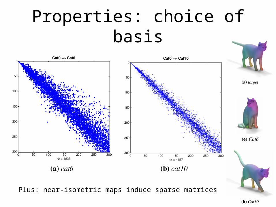
Properties: choice of basis
• Laplace-Beltrami eigenfunctions as the basis
• Although individual eigenfunctions are unstable, space of functions spanned is “stable”
Properties: choice of basis
• Compare two discretizations of the Laplace-Beltrami operator [Meyer et al. 2002]– With and without area normalization
Properties: choice of basis
Meshes: 27.8K points
Good qualityWith a 40x40 matrix, we have 17 times memory savings over a permutation of size 27.8K
Properties: choice of basis
Plus: near-isometric maps induce sparse matrices
Properties: continuity
• Naturally handles map continuity• Three types of continuity:– Changes of the input functionImage varies continuously under changes of a– Image functionLaplace-Beltrami is well-suited for smooth functions is smooth– Representation• Any matrix C is a functional mapping
Properties: continuity
Mapping obtained using an interpolation between two maps: C = C1 + (1- )C2
• Landmark point correspondences– Use f(x) that is distance function to the landmark
• Segment correspondences– Also distance functions or indicator functions
Properties: operator commutativity
• W.r.t. linear operators on the shapes– E.g., symmetry
• An example– C is a map between a man and a woman– RF ,SF is the map the left hand to right hand on the
woman and man, respectively– Man ->Woman, Woman left->Woman right Man left -
> Woman right– Man left -> Man Right Man -> Woman Man Left ->
Woman Right
Properties: regularization constraints
• Not every matrix C is a point-to-point map• It is most meaningful to consider orthonormal
or nearly-orthonormal functional matrices
Map inversion and composition
• Finding an inverse of a map that is not a bijection can be challenging
• In the functional case, an inverse is given simply by the inverse of the matrix C
• A good approximation is the transpose of C
• Composition becomes matrix multiplication
Functional map inference
• Construct a large system of equations• Each equation is one constraint• Constraint for function preservation• Find the matrix C that satisfies the constraints• In fact, we will need many constraints to
obtain C in a least-squares sense• Thus, we need candidate point-to-point or
segment-to-segment correspondences
Map refinement and conversion
• Refine C and convert to a point-to-point map
• For each point x is the source embedding• Find closest point x’ in the target embedding• Find the optimal C by minimizing |Cx – x’|• Iterate this procedure
• Similar to spectral matching [Jain et al. 2007]• Differences
– Good initial estimate C– “Mixing” across eigenvectors
Applications: shape matching
• Compute Laplace-Beltrami eigenfunctions• Compute shape descriptors (WKS)• Compute segment correspondences• Add constraints into a linear system and solve• Refine the solution C• Obtain point-to-point correspondences
Applications: shape matching
• Applied on the benchmark of Kim et al. 2011
Examples of correspondences obtained
Applications: shape matching
Correspondence results on two datasets
Applications: map improvement
• The strength lies on the representation itself• Take point-to-point maps computed by the
other methods• Improve the maps with the functional maps• Adds regularization• Takes 15s for 50K point mesh in 3GHz CPU
Applications: map improvement
Color shows location of errors
Applications: map improvement
Color shows location of errors
Applications: map improvement
Evaluation on the benchmark
Applications: shape collections
• Iteratively Corrected Shape Maps (ICSM) [Nguyen et al. 2011] – compose maps on cycles L→M →N →L– Compare result to the identity map
• Map diffusion [Singer and Wu 2011]– construct a “SuperMap” for the whole collection,– replace a map with a weighted average of other
maps
Applications: shape collections
ICSM applied on the SCAPE dataset using the functional mapsEach entry is the average geodesic map between 11 shapes
Applications: shape collections
Geodesic errors of the mappings in this dataset
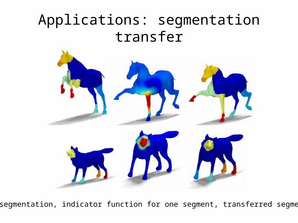
Applications: segmentation transfer
• Functional maps reduce the transfer of functions to matrix multiplication
• Without resorting to point-to-point maps
• Use indicator functions for segments• Perform matrix multiplication• Transform attributes into a “hard” clustering
Applications: segmentation transfer
Source segmentation, indicator function for one segment, transferred segmentation
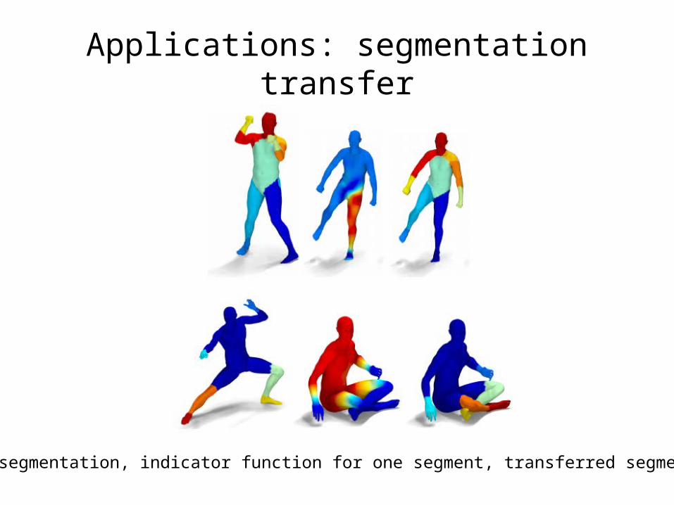
Applications: segmentation transfer
Source segmentation, indicator function for one segment, transferred segmentation
Conclusion
• Novel representation of maps between shapes• Generalizes point-to-point maps• Constraints become linear
• More general classes of deformations?– Optimal choice of basis
Discussion
• In practice, could pose the method as: “find a correspondence between eigenfunctions”? Actually, People has used spectral basis to compute the shape map– JAIN, V., ZHANG, H., AND VAN KAICK, O. 2007. Non-rigid spectral
correspondence of triangle meshes. International Journal on Shape Modeling 13, 1, 101–124
– MATEUS, D., HORAUD, R. P., KNOSSOW, D., CUZZOLIN, F., AND BOYER, E. 2008. Articulated shape matching using Laplacian eigenfunctions and unsupervised point registration. In Proc. CVPR, 1–8.
• What does the representation really bring? a new concept functional map?


![Functional correspondence by matrix completion · Functional maps Let X and Y denote two manifolds sampled at n and m points, respectively. Ovsjanikov et al. [4] propose to model](https://static.documents.pub/doc/80x56/5f51bb7b898a4b2f9a4e3299/functional-correspondence-by-matrix-completion-functional-maps-let-x-and-y-denote.jpg)

