Page 1
Louisiana State UniversityLSU Digital Commons
LSU Historical Dissertations and Theses Graduate School
2000
Fundamental Characterization and NumericalSimulation of Large Stone Asphalt Mixtures.Baoshan HuangLouisiana State University and Agricultural & Mechanical College
Follow this and additional works at: https://digitalcommons.lsu.edu/gradschool_disstheses
This Dissertation is brought to you for free and open access by the Graduate School at LSU Digital Commons. It has been accepted for inclusion inLSU Historical Dissertations and Theses by an authorized administrator of LSU Digital Commons. For more information, please [email protected] .
Recommended CitationHuang, Baoshan, "Fundamental Characterization and Numerical Simulation of Large Stone Asphalt Mixtures." (2000). LSU HistoricalDissertations and Theses. 7367.https://digitalcommons.lsu.edu/gradschool_disstheses/7367
Page 2
INFORMATION TO USERS
This manuscript has been reproduced from the microfilm master. UMI films the
text directly from the original or copy submitted. Thus, some thesis and
dissertation copies are in typewriter face, while others may be from any type of
computer printer.
The quality of th is reproduction is dependen t upon the quality of the copy
subm itted . Broken or indistinct print, colored or poor quality illustrations and
photographs, print bleedthrough, substandard margins, and improper alignment
can adversely affect reproduction.
In the unlikely event that the author did not send UMI a complete manuscript and
there are missing pages, these will be noted. Also, if unauthorized copyright
material had to be removed, a note will indicate the deletion.
Oversize materials (e.g., maps, drawings, charts) are reproduced by sectioning
the original, beginning at the upper left-hand comer and continuing from left to
right in equal sections with small overlaps. Each original is also photographed in
one exposure and is included in reduced form at the back of the book.
Photographs included in the original manuscript have been reproduced
xerographically in this copy. Higher quality 6” x 9” black and white photographic
prints are available for any photographs or illustrations appearing in this copy for
an additional charge. Contact UMI directly to order.
Bell & Howell Information and Learning 300 North Zeeb Road, Ann Arbor, Ml 48106-1346 USA
800-521-0600
Reproduced with permission of the copyright owner. Further reproduction prohibited without permission.
Page 3
Reproduced with permission of the copyright owner. Further reproduction prohibited without permission.
Page 4
FUNDAMENTAL CHARACTERIZATION AND NUMERICAL SIMULATION OF LARGE STONE ASPHALT MIXTURES
A Dissertation
Submitted to the Graduate Faculty o f the Louisiana State University and
Agricultural and Mechanical College in partial fulfillment o f the
requirements for the degree of Doctor o f Philosophy
in
The Department o f Civil and Environmental Engineering
byBaoshan Huang
B.S. Tongji University, Shanghai, China, 1984 M.S. Tongji University, Shanghai, China, 1988
December, 2000
Reproduced with permission of the copyright owner. Further reproduction prohibited without permission.
Page 5
UMI Number: 9998686
___ ®
UMIUMI Microform 9998686
Copyright 2001 by Bell & Howell Information and Learning Company. All rights reserved. This microform edition is protected against
unauthorized copying under Title 17, United States Code.
Bell & Howell Information and Learning Company 300 North Zeeb Road
P.O. Box 1346 Ann Arbor, Ml 48106-1346
Reproduced with permission of the copyright owner. Further reproduction prohibited without permission.
Page 6
ACKNOWLEDGMENTS
I wish to express my deepest appreciation to my advisor, Dr. Louay, N. Mohammad, for
his guidance and encouragement throughout the course of this research. Without his
constant support and enthusiastic participation in the work, this research would not be
finished.
I would also express my appreciations to Dr. G. Wije Wathugala, who served as
my academic advisor for the first three years o f my graduate studies in the LSU.
Special thanks to my committee members, Dr. John Metcalf, Dr. Roger Seals, Dr.
Emir Macari, Dr. Freddy Roberts for their constant encouragement and helpful
suggestions during the course o f this work.
Thanks are also due to Mr. Chris Abadie, the asphalt construction engineer at the
Louisiana Department o f Transportation and Development, who has provided valuable
helps throughout the course o f this study.
In addition, I would like to thank my colleagues and best friends, Amar
Raghavendra, Phillip Graves, Glen Graves, Willie Gueho, Greg Tullier, Chris Schwehn,
for their friendship, encouragement and helps during my stay at the Louisiana
Transportation Research Center (LTRC).
Finally, I wish to express my gratitude for the love o f my family, especially my
wife, Xiaojie, whose constant inspiration and support has always played an important
role throughout the course o f my graduate study in LSU.
ii
Reproduced with permission of the copyright owner. Further reproduction prohibited without permission.
Page 7
TABLE OF CONTENTS
ACKNOW LEDGMENTS..................................................................................................... ii
LIST OF TA B LES................................................................................................................ vii
LIST OF FIG U R ES................................................................................................................ x
ABBREVIATIONS................................................................................................................xvi
ABSTRACT.......................................................................................................................... xviii
CHAPTER 1.INTRODUCTION ................................................................................................................ I
1.1 PROBLEM STATEMENT .......................................................................... I1.1.1 Rutting in Asphalt Pavem ents...................................................... 21.1.2 Moisture Damage or Stripping in Asphalt Pavem ents............... 41.1.3 Proposed Louisiana Solution o f LS A M ....................................... 6
1.2 BACKGROUND AND LITERATURE R EV IE W .................................... 71.2.1 Large Stone Asphalt M ixtures...................................................... 71.2.2 Review o f Recent Applications o f L S A M ................................... 81.2.3 Benefits o f LSAM ....................................................................... 111.2.4 Latest Development o f LSAM R esearch.................................. 131.2.5 Numerical Simulations o f Pavement S tructu re ........................ 16
1.3 LIMITATIONS OF EXISTING PROCEDURES................................... 181.4 SIGNIFICANCE OF THIS R E SE A R C H ................................................ 18
CHAPTER 2.OBJECTIVE AND S C O P E ................................................................................................. 20
2.1 OBJECTIVE ................................................................................................ 202.2 S C O PE ........................................................................................................... 21
CHAPTER 3.METHODOLOGY .............................................................................................................. 23
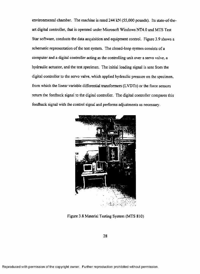
3.1 Facilities......................................................................................................... 233.1.1 Specimen Preparation F acility .................................................... 233.1.2 Mixture Performance Test Facility ........................................... 27
3 .1.2.1 Materials Testing System (MTS Model 810) .............. 273.1.2.2 Cox and Son CS7500 Axial Testing S y s tem ................ 293.1.2.3 Cox and Son CS7000 Superpave Shear T e s te r 303.1.2.4 Asphalt Pavement A nalyzer............................................ 323.1.2.5 LTOC Dual Mode Perm eam eter.................................... 32
3.1.3 Computational Facility ............................................................... 353.2 M ATERIALS................................................................................................ 35
3.2.1 Asphalt B in d e r.............................................................................. 35
iii
Reproduced with permission of the copyright owner. Further reproduction prohibited without permission.
Page 8
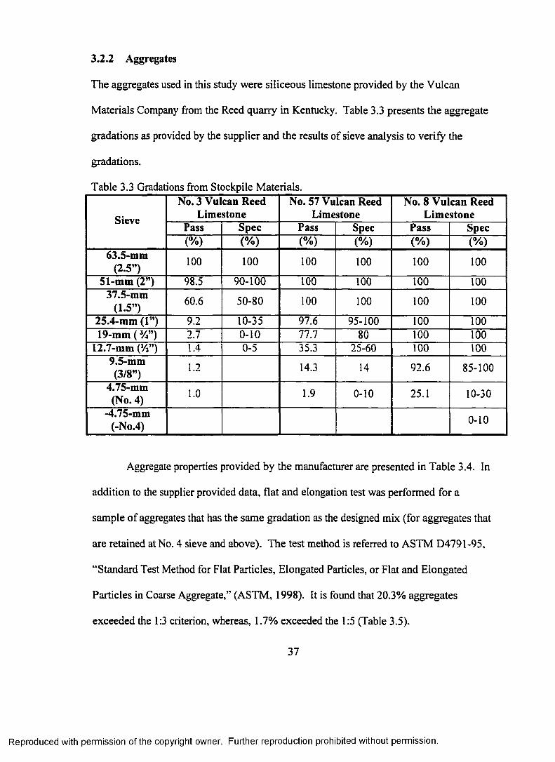
3.2.2 Aggregates..................................................................................... 373.3 DEVELOPMENT OF MIXTURE DESIGN ........................................ 38
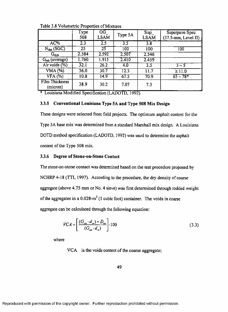
3.3.1 Mixture Gradations ...................................................................... 383.3.2 LSAM Bulk Specific Gravity Test ............................................ 433.3.3 Open-graded LSAM Design ....................................................... 463.3.4 Superpave LSAM Design ........................................................... 463.3.5 Conventional Louisiana Type 5A and Type 508 Mix Design . 493.3.6 Degree of Stone-on-Stone Contact ............................................ 49
3.4 DEVELOPMENT OF TEST FA C TO R IA LS........................................ 523.5 MIXTURE PERFORMANCE CHARACTERIZATION..................... 53
3.5.1 Specimen Preparation .................................................................. 533.5.2 Indirect Tensile Resilient Modulus (Mr) T e s t ........................... 543.5.3 Indirect Tensile Strength (ITS) and Strain T e s t......................... 573.5.4 Axial Creep Test ........................................................................... 593.5.5 Indirect Tensile Creep Test ......................................................... 623.5.6 APA Rut T es t................................................................................. 623.5.7 Superpave Frequency Sweep at Constant Height (FSCH). . . . 673.5.8 Superpave Repetitive Shear at Constant Height (RSCH) . . . . 703.5.9 Moisture Susceptibility Test ....................................................... 723.5.10 Permeability T e s t ........................................................................... 743.5.11 Draindown T e s t ............................................................................. 75
3.6 FUNDAMENTALS OF PERMEABILITY IN ASPHALTM IXTURES............................................................................................... 753.6.1 Fundamentals o f Hydraulic C onductivity .................................. 76
3.6.1.1 Darcy’s L a w ...................................................................... 763.6.1.2 Theoretical Determination o f Darcy’s Hydraulic
Conductivity...................................................................... 783.6.1.3 Range of Validity o f Darcy’s L aw ................................. 81
3.6.2 Laboratory Test to Measure Hydraulic Conductivity .............. 833.6.2.1 Test M ethods................................................................... 833.6.2.2 Test Concerns................................................................... 83
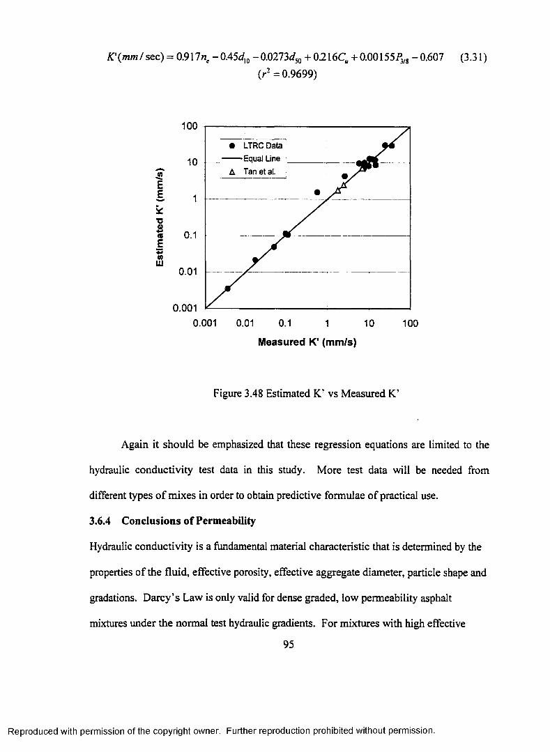
3.6.3 Laboratory Study of Hydraulic Conductivity forAsphalt M ixtures.......................................................................... 843.6.3.1 Objectives ........................................................................ 843.6.3.2 Dual Mode Perm eam eter................................................ 853.6.3.3 Materials .......................................................................... 853.6.3.4 Effective Porosity ( n j .................................................... 873.6.3.5 Test Data P ro cessing ...................................................... 883.6.3.6 Analysis o f Test R esults.................................................. 913.6.3.7 Estimation of Hydraulic Conductivity.......................... 93
3.6.4 Conclusions of Permeability ....................................................... 95
CHAPTER 4.ANALYSIS OF MIXTURE TEST R E SU L T S............................................................... 97
4.1 VOLUMETRIC PROPERTIES................................................................ 97
iv
Reproduced with permission of the copyright owner. Further reproduction prohibited without permission.
Page 9
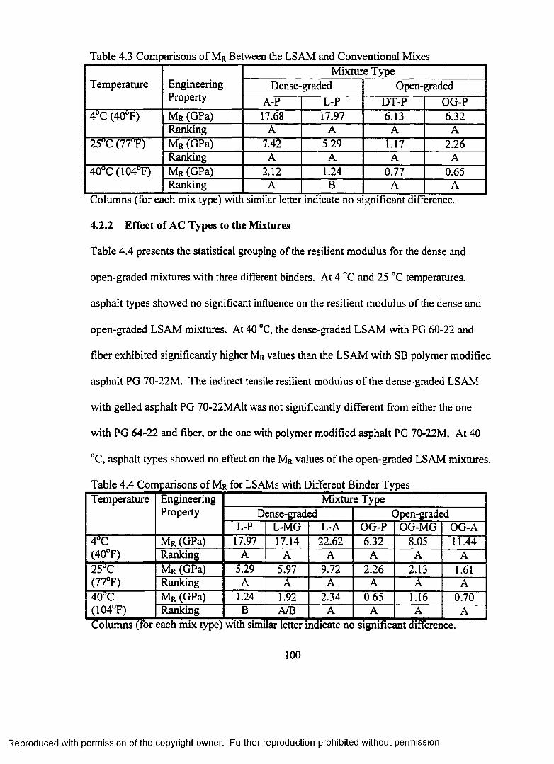
4.2 ELASTIC PROPERTIES ......................................................................... 984.2.1 Comparison between LSAM and Conventional Mixtures . . . . 994.2.2 Effect of AC Types to the M ixtures......................................... 100
4.3 PERMANENT DEFORMATION PROPERTIES ............................. 1014.3.1 Axial Creep Test ........................................................................ 1014.3.2 Indirect Tensile Creep Test ...................................................... 1024.3.3 Superpave Simple Shear Frequency Sweep at Constant
Height (FSC H )............................................................................. 1044.3.4 Superpave Simple Shear Repetitive Shear at Constant
Height (RSCH)............................................................................ 1104.3.5 APA Rut T e s t............................................................................... 1124.3.6 Summary of Permanent Deformation Properties.................... 116
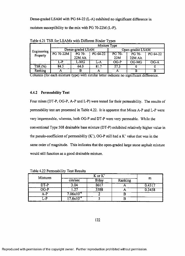
4.4 MOISTURE SUSCEPTIBILITY PROPERTIES ................................ 1194.4.1 Moisture Susceptibility (Modified Lottman) Test ............... 1204.4.2 Permeability T e s t ........................................................................ 122
4.5 MIXTURE DURABILITY PROPERTY ............................................ 1234.5.1 Indirect Tensile Strength and Strain T est................................ 123
4.6 DRAIN-DOWN SUSCEPTIBILITY..................................................... 1244.7 SUMMARY OF MIXTURE CHARACTERIZATION ..................... 1254.8 APPLICATIONS OF MIX CHARACTERIZATION TO
PAVEMENT PERFORMANCE PREDICTION .............................. 128
CHAPTER 5.DEVELOPMENT OF 3-D DYNAMIC FINITE ELEMENT PROCEDURE 130
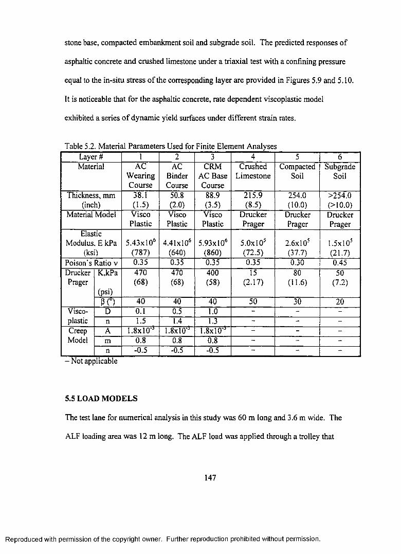
5.1 PREVIOUS STUDIES.............................................................................. 1305.2 OBJECTIVES AND S C O P E ................................................................... 1325.3 GEOMETRIC MODELS FOR THE FINITE ELEMENT
ANALYSES............................................................................................. 1335.4 MATERIAL MODELS FOR THE FINITE ELEMENT
ANALYSES............................................................................................. 1415.4.1 Rate-Dependent Viscoplastic M o d e l....................................... 1415.4.2 Elastoplastic Model (Drucker-Prager Model) ........................ 1455.4.3 Material Param eters.................................................................... 145
5.5 LOAD MODELS...................................................................................... 1475.6 NUMERICAL SIMULATION OF A L F .............................................. 153
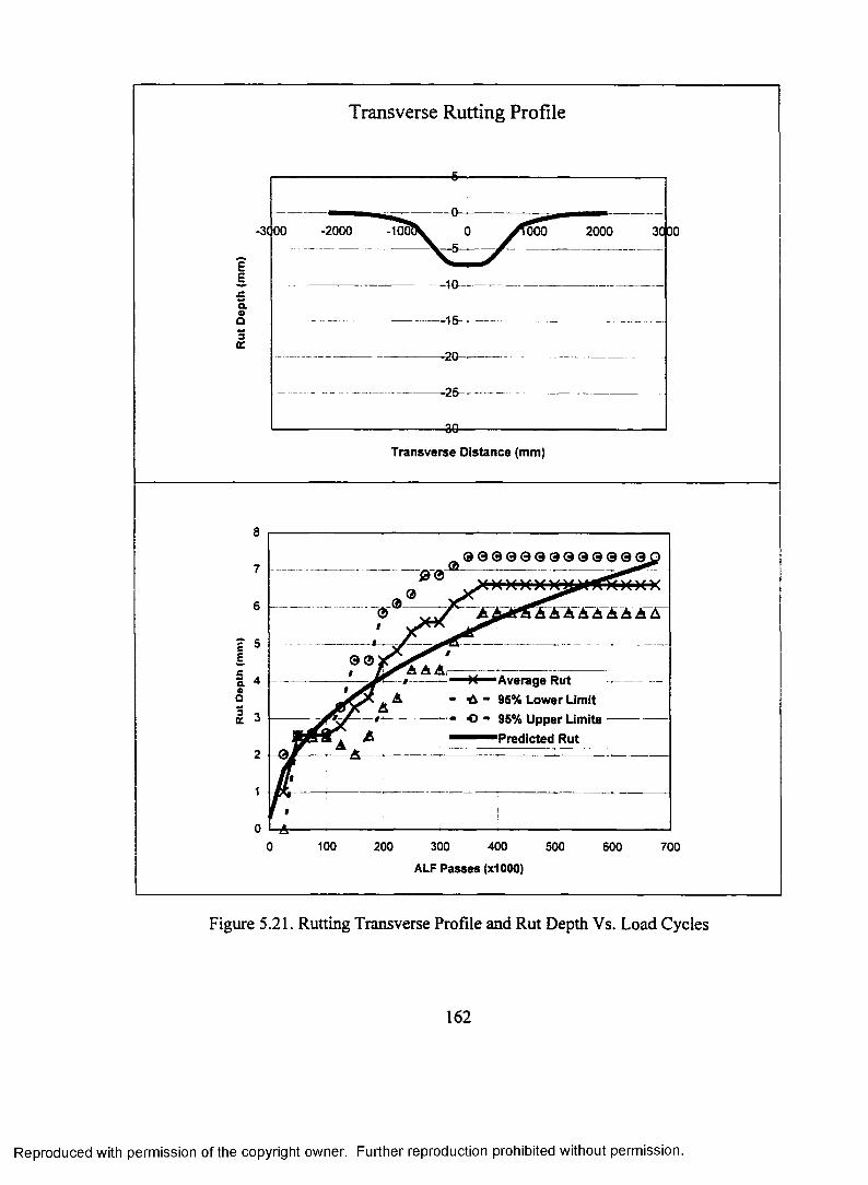
5.6.1 Pavement Surface D eflections................................................. 1555.6.2 Stresses and S tra in s .................................................................... 1555.6.3 Permanent Deformation (R u ttin g )........................................... 160
5.7 SUMMARY OF DEVELOPMENT OF 3-D FEM PROCEDURE . . 160
CHAPTER 6.FINITE ELEMENT COMPARISONS OF PAVEMENTS CONTAININGLSAM AND CONVENTIONAL ASPHALT MIXTURES ....................................... 164
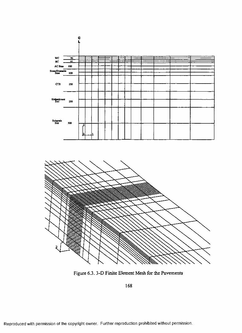
6.1 PAVEMENT STRUCTURES FO R COMPARISON.......................... 1646.2 FINITE ELEMENT GEOMETRIC M E SH .......................................... 165
v
Reproduced with permission of the copyright owner. Further reproduction prohibited without permission.
Page 10
6.3 MATERIAL PARAM ETERS................................................................ 1696.4 COMPARISONS OF SIMULATED PAVEMENT RESPONSES . . 169
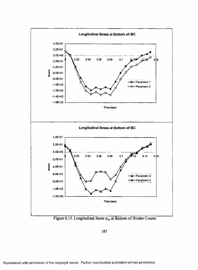
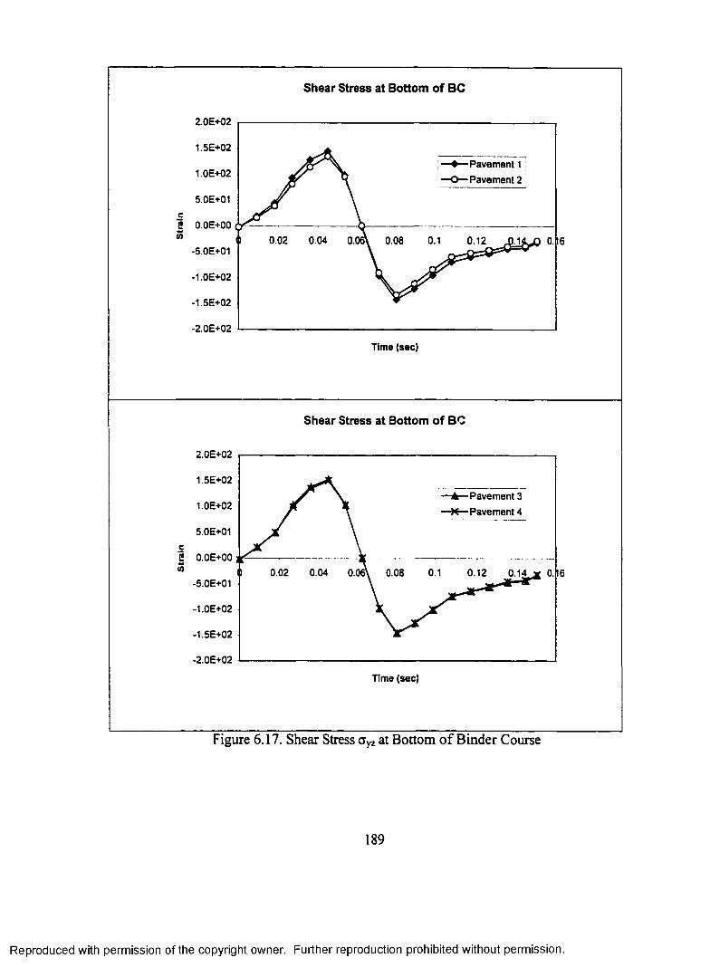
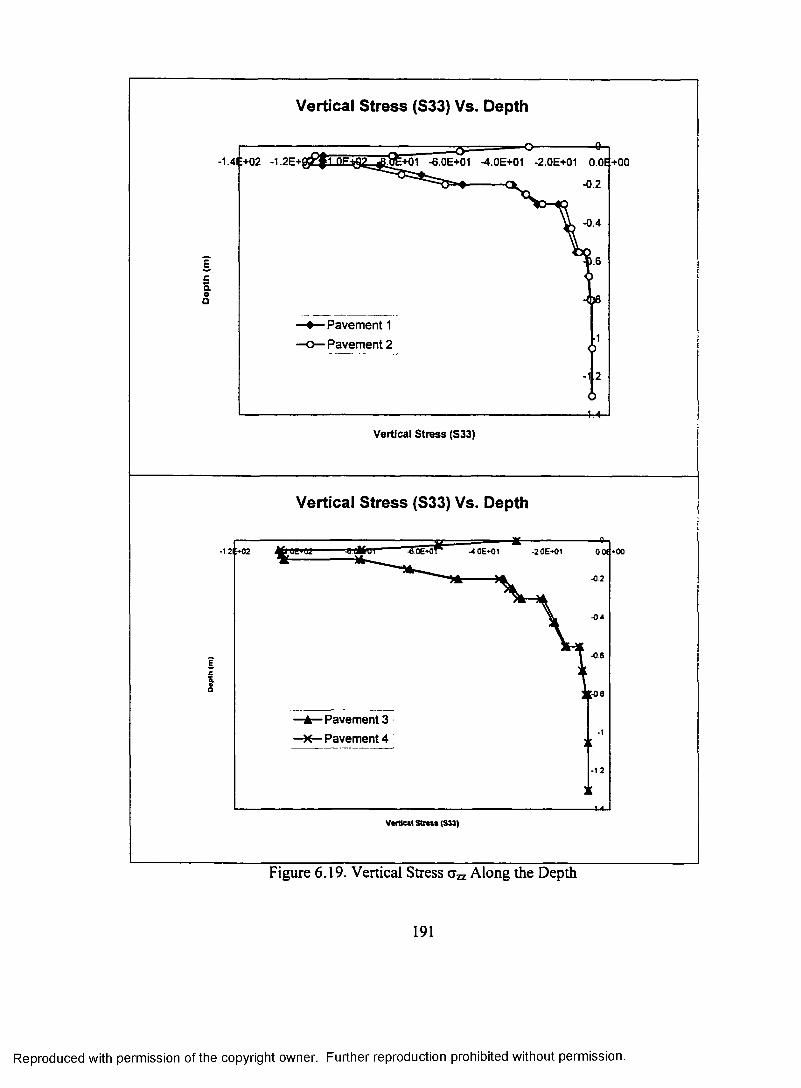
6.4.1 D eflections................................................................................... 1696.4.2 Strains ......................................................................................... 1726.4.3 S tresses ......................................................................................... 183
6.5 SUMMARY OF NUMERICAL STRUCTURAL COMPRISONS . 184
CHAPTER 7.SUMMARY AND CONCLUSIONS ............................................................................ 194
REFERENCES .................................................................................................................. 197
VITA ................................................................................................................................... 203
vi
Reproduced with permission of the copyright owner. Further reproduction prohibited without permission.
Page 11
LIST OF TABLES
Table 1.1 Responses from 52 Highway Specifying Agencies onLSAM (TTI, 1997) 10
Table 1.2 Comparisons o f Previous Researches and This Research .................. 19
Table 2.1 Eight Mixtures Designed in this Study ................................................... 21
Table 3.1 Minimum SST System Requirem ents..................................................... 31
Table 3.2 LaDOTD Performance Graded Asphalt Cement Specification& Test R e su lts ............................................................................................ 36
Table 3.3 Gradations from Stockpile M aterials....................................................... 37
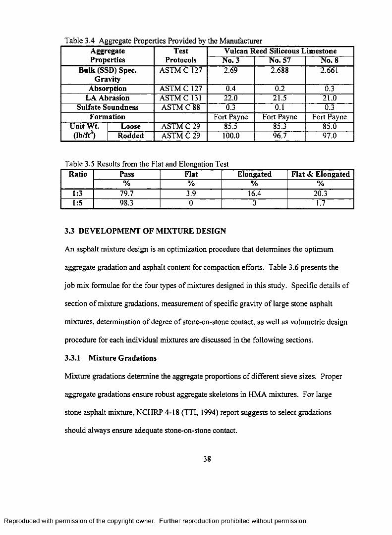
Table 3.4 Aggregate Properties Provided by the M anufacturer............................. 38
Table 3.5 Results from the Flat and Elongation T es t............................................... 38
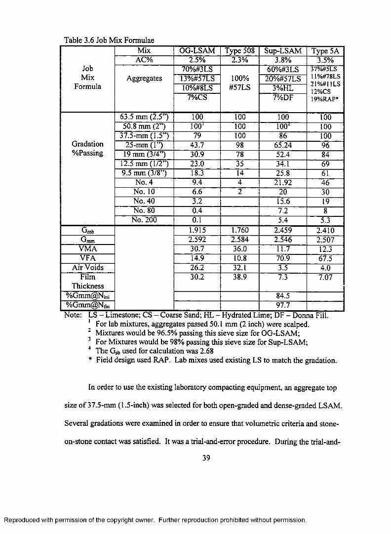
Table 3.6 Job Mix F o rm u la ........................................................................................ 39
Table 3.7 Volumetric Properties o f Open-graded LSAM at DifferentAsphalt Contents ....................................................................................... 47
Table 3.8 Volumetric Properties of Mixtures ....................................................... 49
Table 3.9 VCA and Degree o f Stone-on-Stone Contact ........................................ 51
Table 3.10 Mixture Performance T e s ts ....................................................................... 52
Table 3.11 Mix Asphalt Content and Other Gradation Param eters......................... 87
Table 3.12 Hydraulic Conductivity Test R esu lts ........................................................ 91
Table 3.13 Reynolds Number for Different Mixes at / = / ...................................... 92
Table 4.1 Mixtures Evaluated .................................................................................... 97
Table 4.2 Volumetric Properties o f Mixtures .......................................................... 98
Table 4.3 Comparisons o f MR Between the LSAM and Conventional Mixes . . 100
Table 4.4 Comparisons o f M R for LSAMs with Different Binder Types .......... 100
vii
Reproduced with permission of the copyright owner. Further reproduction prohibited without permission.
Page 12
Table 4.5 Axial Creep Test for Dense-graded and Open-graded Mixtures . . . . 101
Table 4.6 Axial Creep Test for LSAMs with Different Binder Type ................. 102
Table 4.7 Indirect Tensile Creep Test Results o f Open and Dense-graded Mixes ................................................................................... 103
Table 4.8 Indirect Tensile Creep Test Results for LSAMs withDifferent Binder Types .......................................................................... 103
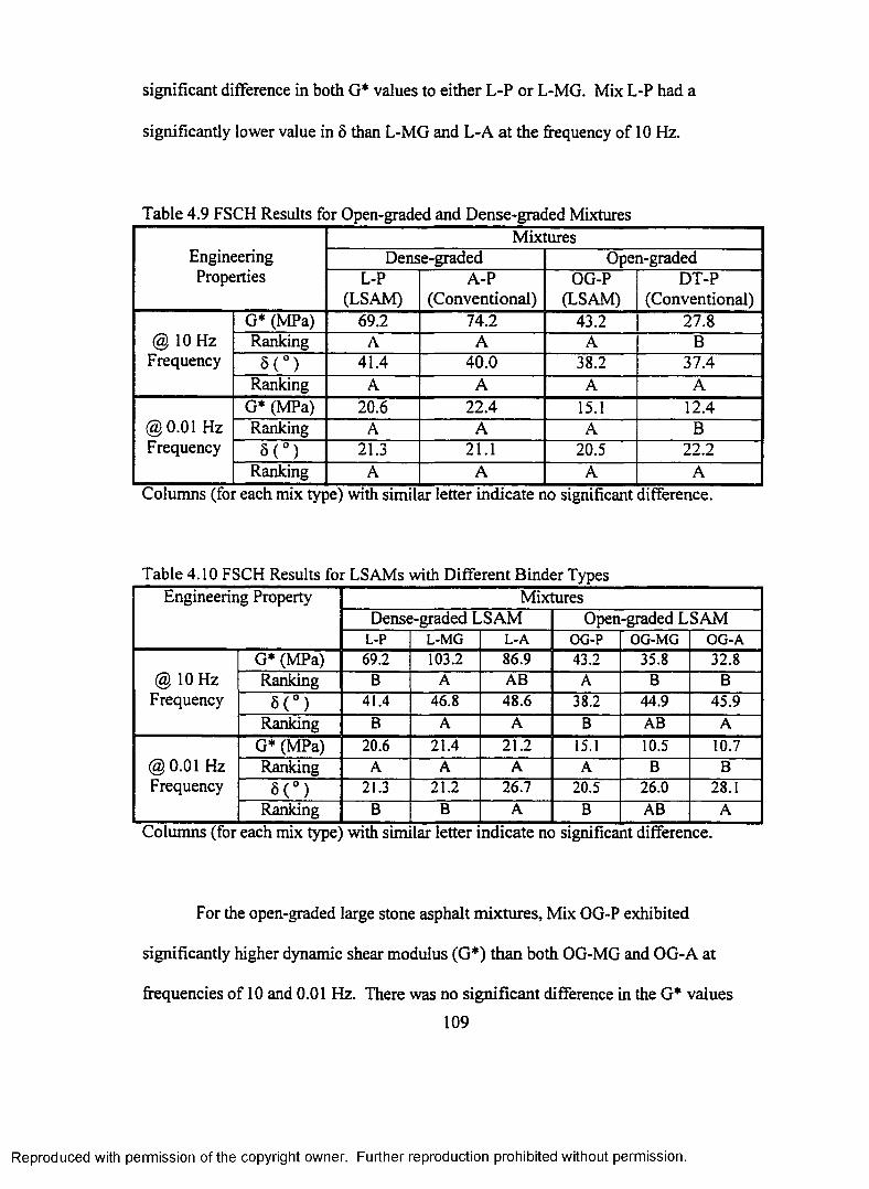
Table 4.9 FSCH Results for Open-graded and Dense-graded M ix tu res 109
Table 4.10 FSCH Results for LSAMs with Different Binder T y p es ..................... 109
Table 4.11 Permanent Shear Strain at 5000 Cycles o f RSCH T e s t ........................ I l l
Table 4.12 Permanent Shear Strain at 5000 Cycles o f RSCH Test forLSAMs with Different AC B inders....................................................... 112
Table 4.13 APA Rut Depth at 8000 Cycle for Dense and Open-graded Mixtures ....................................................................................... 115
Table 4.14 APA Rut Depth at 8000 Cycles for LSAMs with DifferentBinder Types ....................................................................................... 116
Table 4.15 Rut Susceptibility of Dense-graded Mixtures ....................................... 117
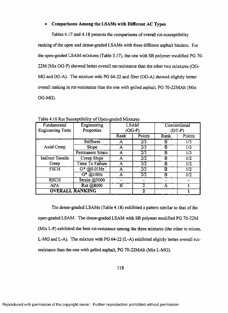
Table 4.16 Rut Susceptibility o f Open-graded M ixtures......................................... 118
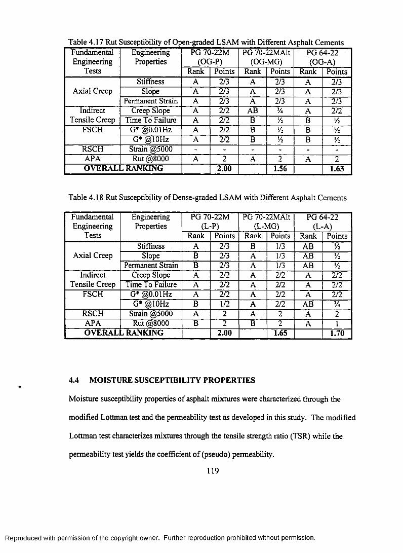
Table 4.17 Rut Susceptibility of Open-graded LSAMs with DifferentAsphalt Cements ..................................................................................... 119
Table 4.18 Rut Susceptibility of Dense-graded LSAMs with DifferentAsphalt Cements ..................................................................................... 119
Table 4.19 Modified Lottman Test R esu lts ............................................................... 120
Table 4.20 Comparison of TSR for LSAM and Conventional M ixtures 121
Table 4.21 TSR for LSAMs with Different Binder Types ..................................... 122
Table 4.22 Permeability Test Results ........................................................................ 122
Table 4.23 Indirect Tensile Strength (ITS) Test Results o f Dense andOpen-graded M ixtures............................................................................ 124
viii
Reproduced with permission of the copyright owner. Further reproduction prohibited without permission.
Page 13
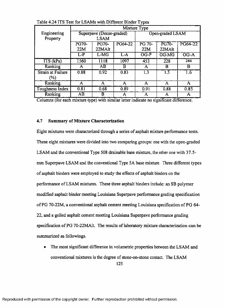
Table 4.24 ITS Test for LSAMs with Different Binder T y p e s ............................. 125
Table 5.1 Scope of FE Analysis................................................................................ 132
Table 5.2 Material Parameters Used for Finite Element Analyses ..................... 147
Table 6.1 Material Parameters Used in the Structural Comparisonsfor Pavement 1 .......................................................................................... 170
Table 6.2 Material Parameters Used in the Structural Comparisonsfor Pavement 2 .......................................................................................... 170
Table 6.3 Material Parameters Used in the Structural Comparisonsfor Pavement 3 .......................................................................................... 171
Table 6.3 Material Parameters Used in the Structural Comparisonsfor Pavement 4 .......................................................................................... 171
ix
Reproduced with permission of the copyright owner. Further reproduction prohibited without permission.
Page 14
LIST OF FIGURES
Figure l .l A Typical Pavement Section of Flexible Pavement ................................ 2
Figure 1.2 Mechanisms o f Asphalt Pavement R u ttin g ................................................ 3
Figure 1.3 Severe Stripping o f a HMA Base Course (from Roberts et al, 1994) . . 5
Figure 1.4 Large Stone Asphalt Mixture and Conventional Mixture ....................... 8
Figure 1.5 Number o f LSAM Pavements Constructed Between 1987and 1997 ......................................................................................................... 9
Figure 1.6 Performance o f LSAM as Compared to Conventional M ix tu res............ 9
Figure 1.7 Stone-on-Stone Contact of LSAM ............................................................. 12
Figure 3.1 Mixing Bowl ............................................................................................... 24
Figure 3.2 Mixing B u c k e t............................................................................................. 24
Figure 3.3 PTI Double Pugmill Mixer ....................................................................... 25
Figure 3.4 Pine Instrument Superpave Gyratory Compactor ................................... 25
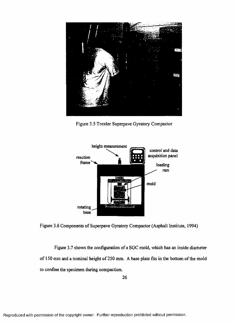
Figure 3.5 Troxler Superpave Gyratory C om pactor.................................................. 26
Figure 3.6 Components o f Superpave Gyratory Compactor(Asphalt Institute, 1994) 26
Figure 3.7 SGC Mold Configuration and Compaction Param eters.......................... 27
Figure 3.8 Material Testing System (MTS 8 1 0 ) ......................................................... 28
Figure 3.9 Closed-loop Controlled Servo-hydraulic Test System .......................... 29
Figure 3.10 Cox and Son CS7500 Axial Texting and Environmental System . . . . 30
Figure 3.11 CS7000 Superpave Shear T e s te r ............................................................... 31
Figure 3.12 Asphalt Pavement Analyzer....................................................................... 33
Figure 3.13 LTRC Dual Mode Permeameter ............................................................... 33
Figure 3.14 Diagram o f LTRC Dual Mode Permeameter............................................ 34
x
Reproduced with permission of the copyright owner. Further reproduction prohibited without permission.
Page 15
Figure 3.15 Gradation Chart o f Four Mixtures in this Study ..................................... 40
Figure 3.16 Gradation Chart o f Large Stone Asphalt Mixtures ................................. 41
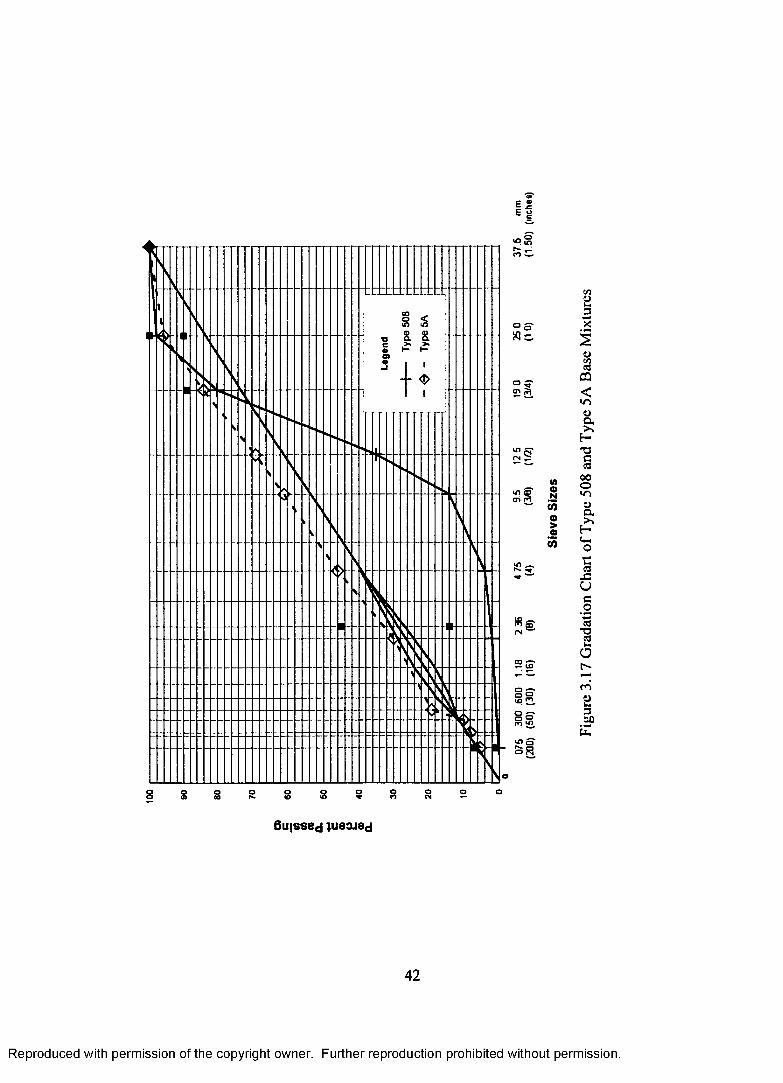
Figure 3.17 Gradation Chart o f Type 508 and Type 5 A Base M ix tures................... 42
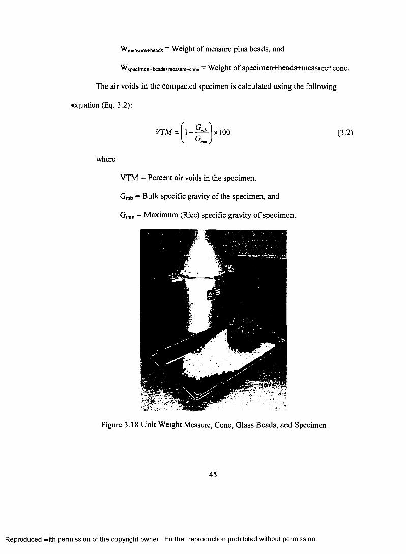
Figure 3.18 Unit Weight Measure, Cone, Glass Beads, and Specimen ................... 45
Figure 3.19 Open-graded LSAM Air V o id s .................................................................. 47
Figure 3.20a Open-graded LSAM VMA ........................................................................ 48
Figure 3.20b Open-graded LSAM V F A .......................................................................... 48
Figure 3.21 Cut-Section Showing Stone-on-Stone Contact ....................................... 51
Figure 3.22 APA Rut Test Cylindrical Samples and M o ld ......................................... 53
Figure 3.23 Test Setup o f Indirect Tensile Resilient Modulus ( M r) T e s t ................. 55
Figure 3.24 Typical IT Resilient Modulus ( M r) Test R esults..................................... 56
Figure 3.25 A Typical Normalized ITS Curve for TI Calculation ............................ 58
Figure 3.26 Test Setup o f Axial Creep Test ................................................................. 60
Figure 3.27 Typical Axial Creep Test Results ............................................................. 61
Figure 3.28 Typical Results from Indirect Tensile Creep T e s t .................................. 63
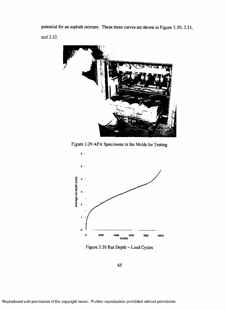
Figure 3.29 APA Specimens in the Molds for T e s tin g ................................................ 65
Figure 3.30 Rut Depth ~ Load C ycles............................................................................ 65
Figure 3.31 Slope - Load Cycles ................................................................................... 66
Figure 3.32 Change o f Slope - Load Cycles................................................................. 66
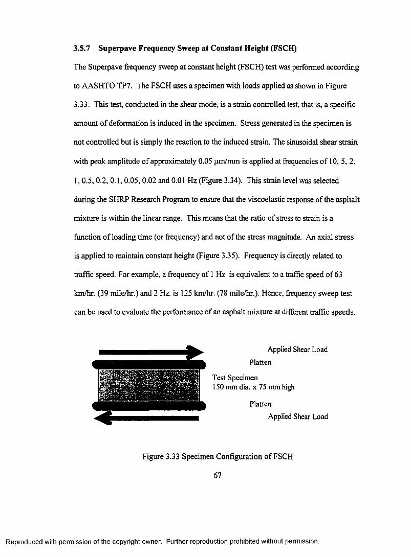
Figure 3.33 Specimen Configuration of F S C H ............................................................. 67
Figure 3.34 Deformation During FSCH (10 Hz) ......................................................... 68
Figure 3.35 Loads During Frequency Sweep at Constant Height Test (10 FIz) . . . 68
xi
Reproduced with permission of the copyright owner. Further reproduction prohibited without permission.
Page 16
Figure 3.36 Complex Shear Modulus (G*) at FSCH Test ....................................... 68
Figure 3.37 Phase Angle (8) at FSCH T e s t.................................................................. 70
Figure 3.38 Haversian Stress Applications in the RSCH Test ................................. 72
Figure 3.39 Darcy’s Experiment ................................................................................. 77
Figure 3.40 Symbols used for Deriving Poiseulle’s Equation ................................. 78
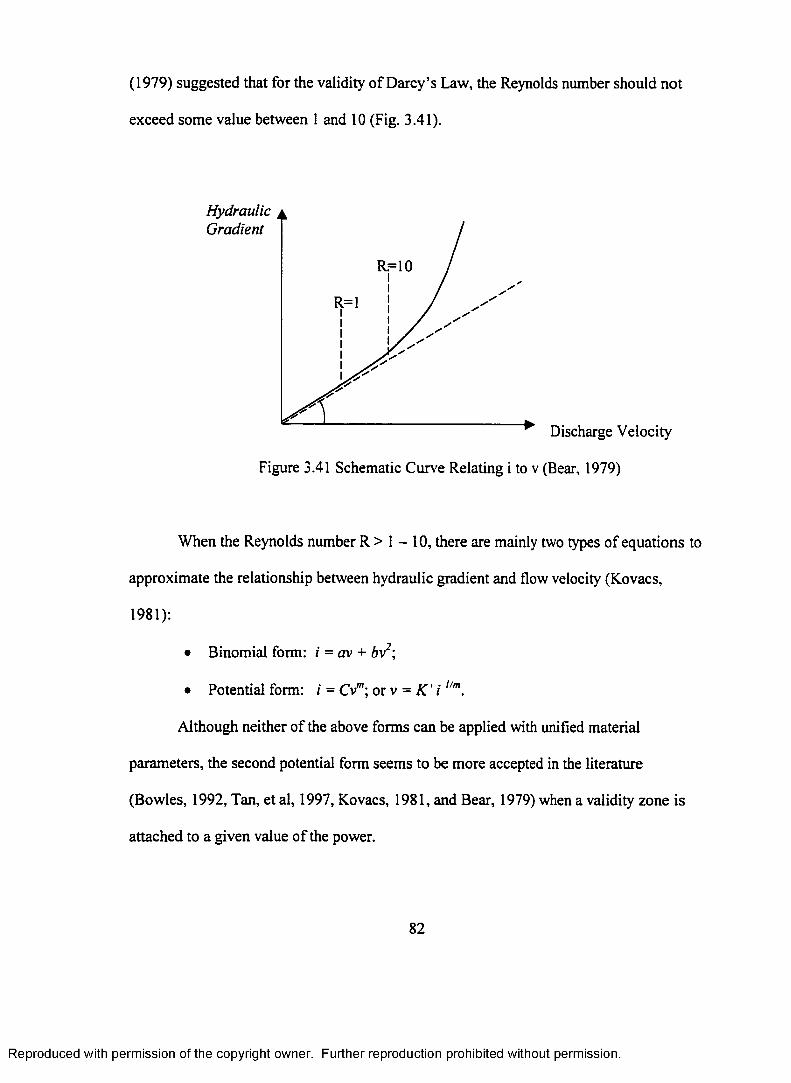
Figure 3.41 Schematic Curve Relation i to v (Bear, 1 9 7 9 )........................................ 82
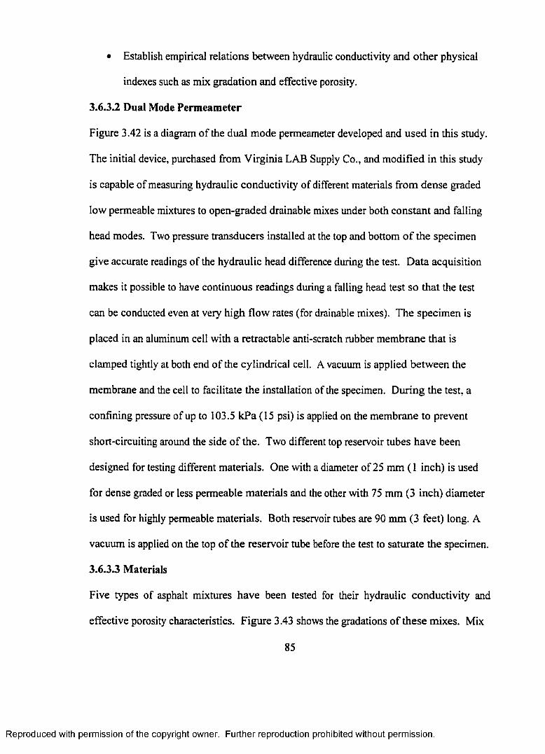
Figure 3.42 Dual Mode Flexible Wall Permeameter................................................... 86
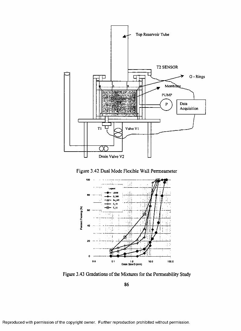
Figure 3.43 Gradations o f the Mixtures for the Permeability S tu d y ......................... 86
Figure 3.44 Hydraulic Head vs. Time in Falling Head T e s t ..................................... 89
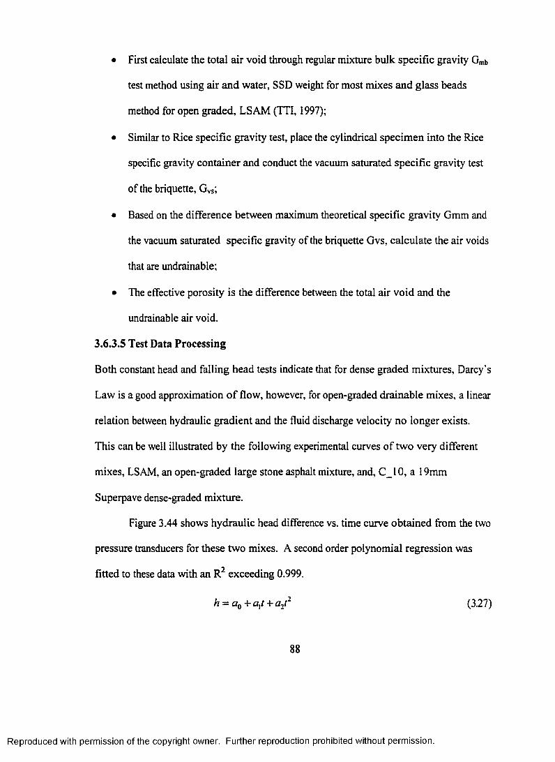
Figure 3.45 Discharge Velocity vs. Hydraulic G rad ien t............................................ 90
Figure 3.46 K.’ vs. Effective P orosity ........................................................................... 92
Figure 3.47 v/i Varies Greatly with Hydraulic Gradient (fromSpecimen D_16)........................................................................................ 93
Figure 3.48 Estimated K’ vs. Measured K.’ .................................................................. 95
Figure 4.1 Average Values of Resilient M odulus..................................................... 99
Figure 4.2 FSCH Dynamic Shear Modulus (G*) o f Open-graded Mixtures . . . 105
Figure 4.3 FSCH Dynamic Shear Modulus (G*) o f Dense-graded Mixtures . . . 106
Figure 4.4 FSCH Phase Angle (8) of Open-graded Mixtures ............................. 107
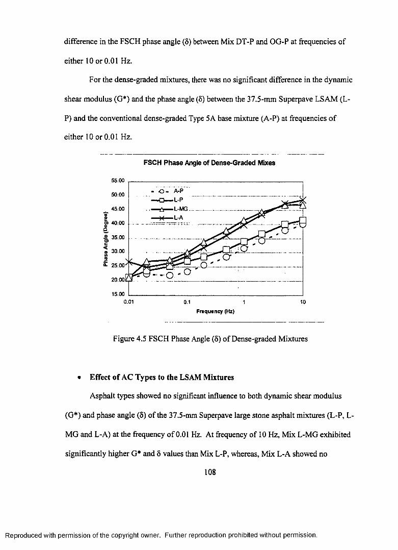
Figure 4.5 FSCH Phase Angle (8) of Dense-graded Mixtures ............................. 108
Figure 4.6 Permanent Shear Strain Vs. Number o f Cycles of RSCH Test . . . . I l l
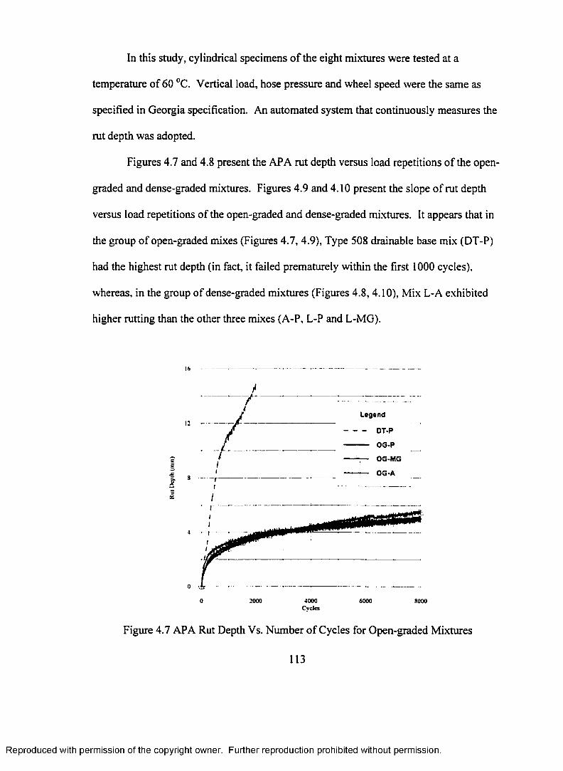
Figure 4.7 APA Rut Depth Vs. Number of Cycles for Open-gradedM ixtures................................................................................................... 113
Figure 4.8 APA Rut Depth Vs. Number o f Cycles for Dense-gradedM ixtures................................................................................................... 114
xii
Reproduced with permission of the copyright owner. Further reproduction prohibited without permission.
Page 17
Figure 4.9 APA Slope Vs. Number of Cycles for Open-graded M ix tu re s 114
Figure 4.10 APA Slope Vs. Number o f Cycles for Dense-graded Mixtures . . . . 115
Figure 5.1 Layout of the Pavement Layers and Instrumentation ofthe Test Lane ............................................................................................ 134
Figure 5.2 2-D Continuum Elements (HKS, 1998)................................................. 135
Figure 5.3 3-D Continuum Elements (HKS, 1998)................................................. 136
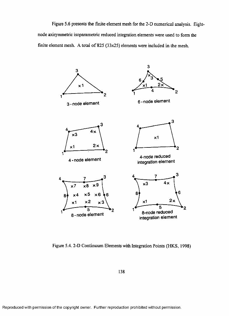
Figure 5.4 2-D Continuum Elements with Integration Points (HKS, 1998) . . . . 138
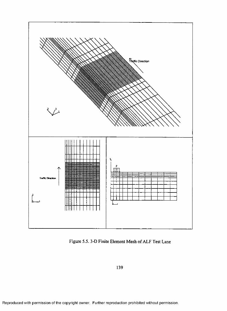
Figure 5.5 3-D Finite Element Mesh of ALF Test L a n e ........................................ 139
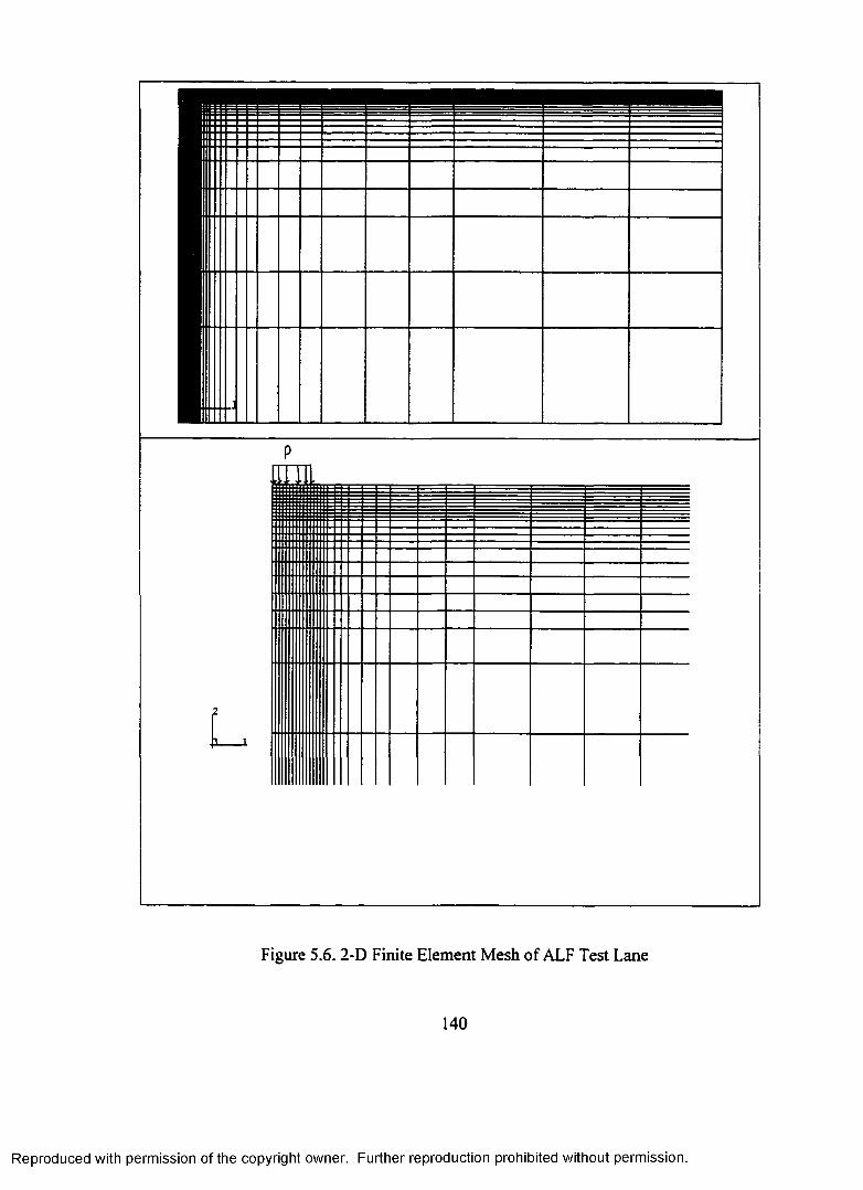
Figure 5.6 2-D Finite Element Mesh of ALF Test L a n e ........................................ 140
Figure 5.7 Elastic Viscoplastic Model ..................................................................... 142
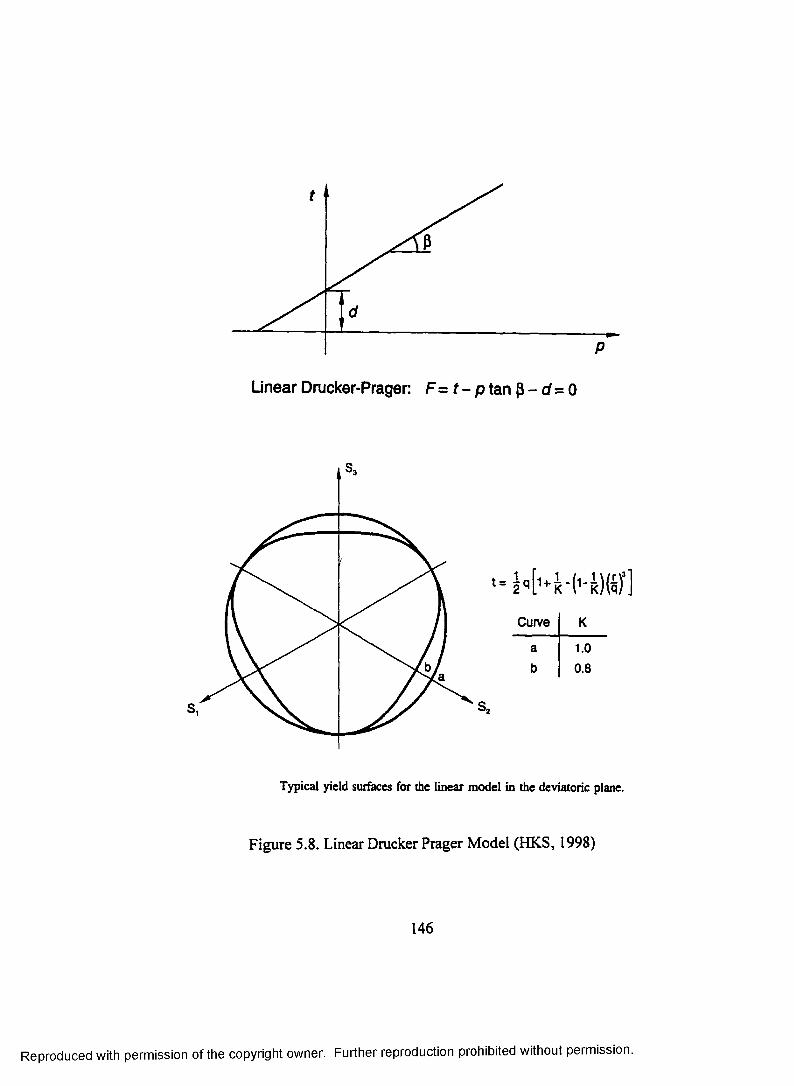
Figure 5.8 Linear Drucker Prager Model (HKS, 1998)........................................... 146
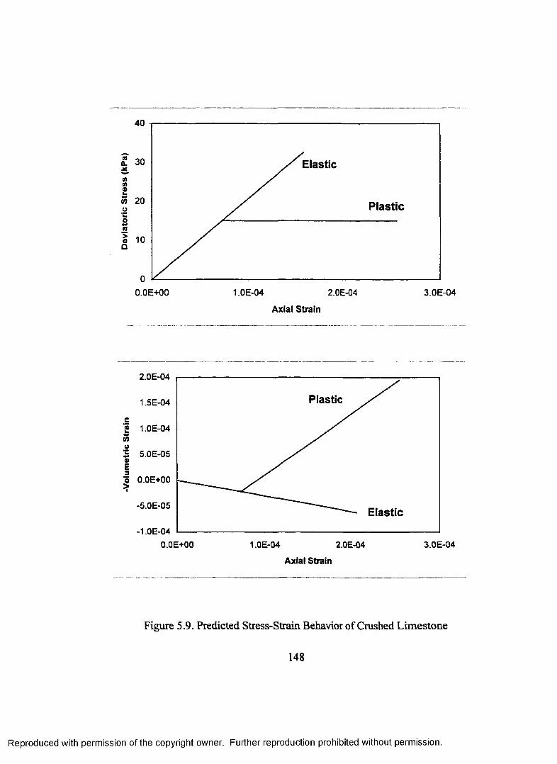
Figure 5.9 Predicted Stress-Strain Behavior o f Crushed L im estone..................... 148
Figure 5.10 Predicted Stress-Strain Behavior o f Asphalt ConcreteWearing Course ............................................................................... 149
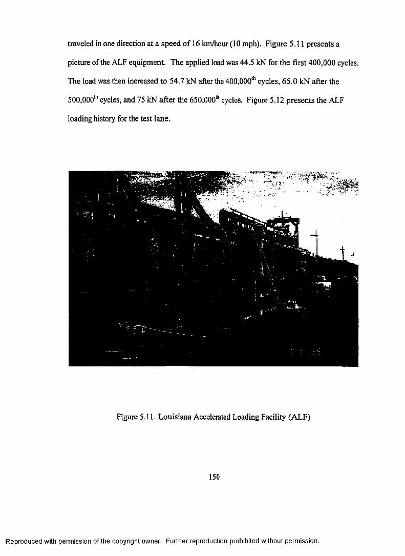
Figure 5.11 Louisiana Accelerated Loading Facility ............................................... 150
Figure 5.12 ALF Loading H istory ................................................................................ 151
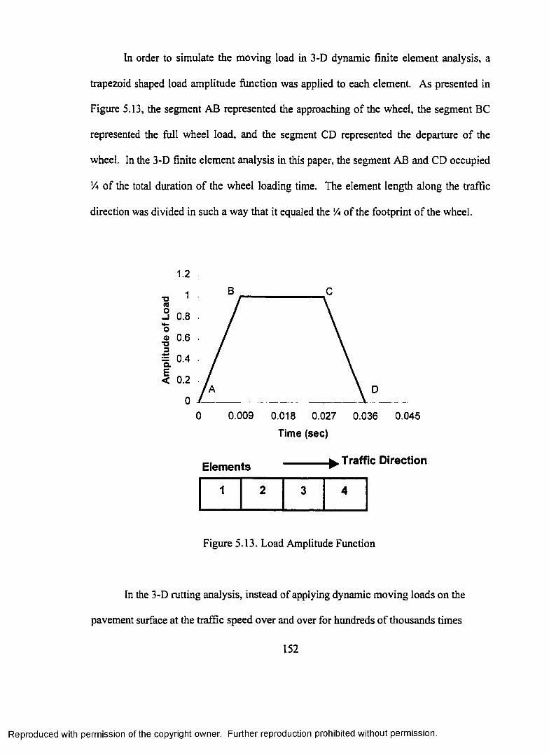
Figure 5.13 Load Amplitude Function ....................................................................... 152
Figure 5.14 Loading Model for 3-D Rutting Analysis ............................................. 154
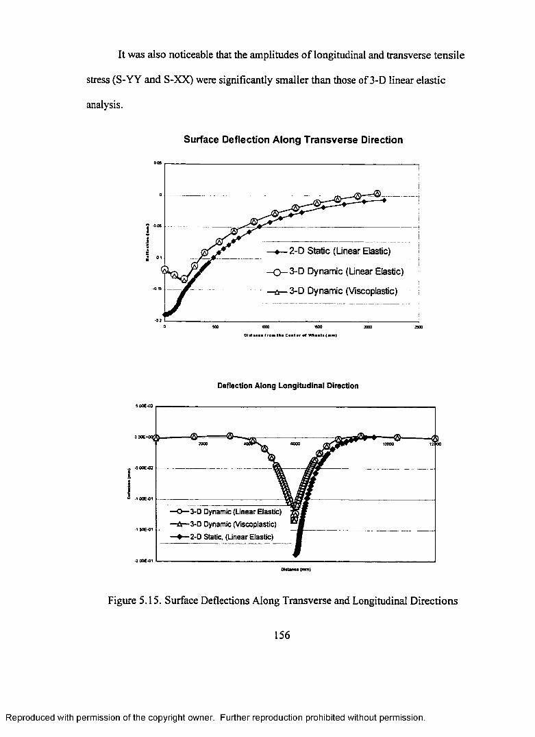
Figure 5.15 Surface Deflections Along Transverse and LongitudinalD irections................................................................................................... 156
Figure 5.16 Stresses at Bottom o f the Asphaltic Concrete, 3-D LinearElastic A n a ly sis ........................................................................................ 157
Figure 5.17 Stresses at Bottom of the Asphaltic Concrete, 3-DViscoplastic Analysis ........................................................................... 158
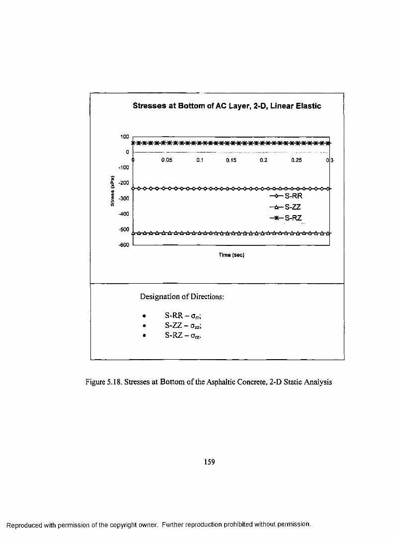
Figure 5.18 Stresses at Bottom o f the Asphaltic Concrete, 2-DStatic A nalysis .......................................................................................... 159
xiii
Reproduced with permission of the copyright owner. Further reproduction prohibited without permission.
Page 18
Figure 5.19 Longitudinal Strain at Bottom o f Surface AC and Asphalt Base . . . 161
Figure 5.20 A Typical Measured Longitudinal Strain Response C u rv e .......... 161
Figure 5.21 Rutting Transverse Profile and Rut Depth Vs. Load C y c le s ........ 162
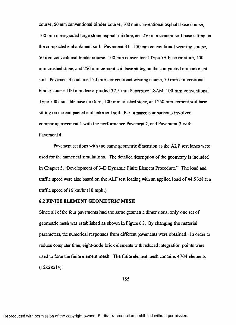
Figure 6.1 Comparisons Between Type 508 Drainable Base andOpen-graded LSAM .............................................................................. 166
Figure 6.2 Comparisons Between Type 5A Base Mix and Dense-graded37.5-mm Superpave L S A M ............................................................ 167
Figure 6.3 3-D Finite Element Mesh for the Pavements.................................. 168
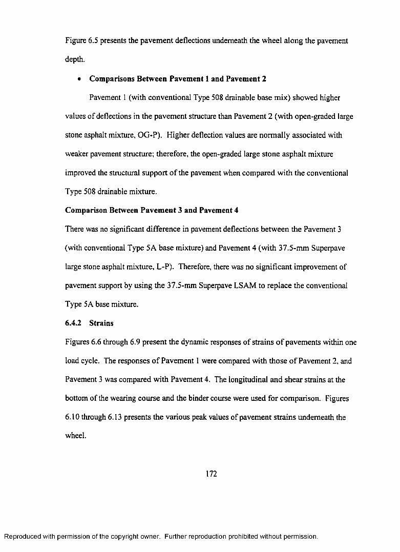
Figure 6.4 Pavement Surface Deflections Along the Transverse Direction . . . . 173
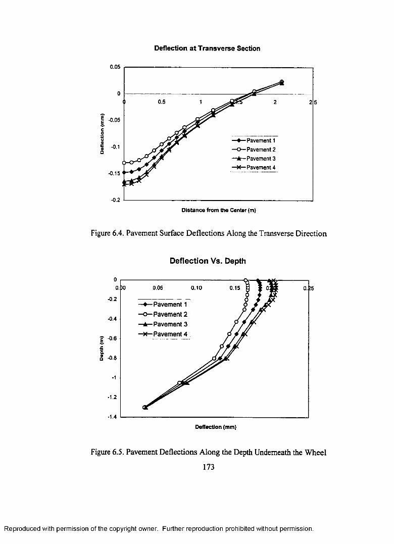
Figure 6.5 Pavement Deflections Along the Depth Underneath the Wheel . . . . 173
Figure 6.6 Longitudinal Strain at Bottom of Wearing C ourse ......................... 174
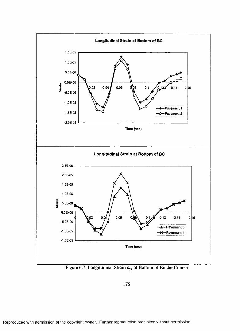
Figure 6.7 Longitudinal Strain &yy at Bottom of Binder Course ........................... 175
Figure 6.8 Shear Strain at Bottom o f Wearing Course...................................... 176
Figure 6.9 Shear Strain £yZ at Bottom o f Binder C ou rse ........................................ 177
Figure 6.10 Longitudinal Strain Along the D ep th ........................................ 178
Figure 6.11 Vertical Strain Along the D e p th ................................................ 179
Figure 6.12 Shear Strain Along the D e p th ............................................................ 180
Figure 6.13 Shear Strain Along the D e p th ............................................................ 181
Figure 6.14 Longitudinal Stress at Bottom of Wearing Course ....................... 186
Figure 6.15 Longitudinal Stress at Bottom of Binder C ourse ........................... 187
Figure 6.16 Shear Stress a n at Bottom o f Wearing Course ..................................... 188
Figure 6.17 Shear Stress at Bottom o f Binder C ourse......................................... 189
Figure 6.18 Longitudinal Stress Along the D epth........................................ 190
xiv
Reproduced with permission of the copyright owner. Further reproduction prohibited without permission.
Page 19
Figure 6.19 Vertical Stress a** Along the D e p th ........................................................ 191
Figure 6.20 Shear Stress Along the D e p th ............................................................ 192
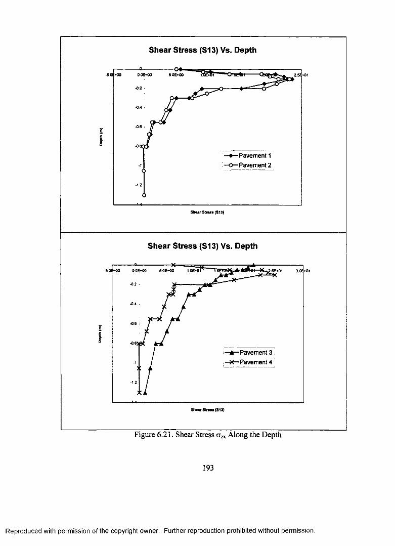
Figure 6.21 Shear Stress Along the D epth ............................................................ 193
xv
Reproduced with permission of the copyright owner. Further reproduction prohibited without permission.
Page 20
ABBREVIATIONS
A = cross-sectional areaAC = asphalt cementALF = accelerated loading facilityAp = area under the normalized stress-strain curve up to strain spAPA = asphalt pavement analyzera e = area under the normalized stress-strain curve up to strain sCu = coefficient o f uniformityD = diameter o f the specimend = diameter o f the particles; Drucker-Prager parameterDCa = density o f coarse aggregateDon = density o f coarse aggregate in the compacted LSAMDh = effective particle diameterdmb = bulk specific gravity of the compacted LSAMdw = density o f waterDOT = department o f transportationE = Young’s elastic moduluse*j = deviatoric strain tensorFEM = finite element methodFHWA = Federal Highway AdministrationFSCH = frequency sweep at constant heightg = acceleration of gravityGca = specific gravity of coarse aggregateGmb = bulk specific gravityOmm = maximum (Rice) specific gravityGTM = gyratory testing machineG* = dynamic complex shear modulush = hydraulic headHt = horizontal deformation at peak loadHMA = hot mix asphalti = hydraulic gradientITS = indirect tensile strengthK = coefficient o f permeability; bulk elastic modulus; ratio o f yield stress
triaxial tension to yield stress in triaxial compressionk = intrinsic permeabilityK’ = pseudo coefficient of permeabilityL = lengthLaDOTD = Louisiana Department of Transportation and DevelopmentLSAM = large stone asphalt mixturesLTRC = Louisiana Transportation Research CenterLWT = loaded wheel testerm = shape factorM r = indirect tensile resilient modulusN = number o f pipes
xvi
Reproduced with permission of the copyright owner. Further reproduction prohibited without permission.
Page 21
n = porosityne = effective porosityP = applied vertical loadPm, = peak loadQ = rate of flowq = Mises equivalent stressR = percent o f coarse aggregate in LSAM; Raynolds number; over stress
ratior = radius; third invariant o f deviatoric stressRAP = recycled asphalt pavementRSCH = repetitive shear at constant heightRSCSR = repetitive shear at constant stress ratioSjj = deviatoric stress tensorSGC = Superpave gyratory compactorSSC = degree of stone-on-stone contactSST = Superpave shear testerSt = tensile strengthStc = average tensile strength o f the control samplesStm = average tensile strength o f the moisture-conditioned samplest = sample thickness; timeTI = toughness indexTSR = tensile strength ratioTTI = Texas Transportation Institutev = velocity o f flowVCA = voids in coarse aggregatesVMA = volume mix asphaltVFA = volume filled with asphalt5H = horizontal deformation5V = vertical deformationa = coefficient o f shape factors = strainsp = strain corresponding to the peak stressst = horizontal tensile strain at failurey = specifc weighty = viscosity parameterr| = viscosity o f the fluid(p = friction anglep = poisson’s ratio; dynamic viscosityv = kinematic viscositycjjj = stress tensor
xvii
Reproduced with permission of the copyright owner. Further reproduction prohibited without permission.
Page 22
ABSTRACT
Large stone asphalt m ixtures (LSAM) are mixtures that contains maximum
aggregate sizes between 25 and 63 mm. LSAMs are used to improve the mixtures’
resistance to rutting and also improve the durability of pavements. However, due to
historical reasons, LSAM has been rarely used in pavement constructions.
The objective o f this study was to determine the fundamental engineering
properties of LSAM for potential use in Louisiana and to conduct numerical
simulations of pavements that contain LSAMs. The scope of this evaluation included
two types LSAMs: an open-graded and a dense-graded 37.5-mm Superpave mix, and
three types of asphalt binders: an SB polymer modified PG 70-22M, a conventional
PG 64-ss, and a gelled asphalt, PG 70-22MAU. The two LSAMs were compared to
their corresponding conventional mixtures: Type 508 and Type 5A. Laboratory
performance tests were conducted to characterize the rut susceptibility, durability,
moisture susceptibility and permeability o f these mixtures.
A three dimensional dynamic finite element procedure was developed during
this study. Advanced material models o f viscoplasticity and elastoplasticity were
incorporated into the 3-D dynamic finite element procedure. This procedure was used
to compare the structural performance of two groups of pavements, each with two
pavements, one with conventional mixtures and one with the LSAM developed in this
study.
The results indicated that the open-graded LSAM developed in this study
exhibited better rut-resistance, durability and moisture susceptibility than the
xviii
Reproduced with permission of the copyright owner. Further reproduction prohibited without permission.
Page 23
conventional LADOTD Type 508 drainable base mixture, whereas the dense-graded
LSAM showed the similar laboratory characteristics to the conventional LADOTD
Type 5A base mixture. Similarly, the numerical simulation indicated that the
pavement containing open-graded LSAM provided increased structural support when
compared to the pavement containing conventional Type 508 drainable mixture,
whereas, the pavement containing the dense-graded LSAM showed no appreciable
increase in structural support comparing to the pavement containing conventional
Type 5 A base mixture.
xix
Reproduced with permission of the copyright owner. Further reproduction prohibited without permission.
Page 24
CHAPTER 1. INTRODUCTION
This document describes the research work and findings o f a laboratory characterization
and numerical analysis o f large stone asphalt mixtures. Chapter 1, the introduction,
includes the problem statement and background information for the research project.
Chapter 2 presents the objective and scope o f the research. Chapter 3 describes the
research methodology for the mixture characterization that includes a brief description of
test equipment, development o f test factorials, the materials used in the study,
development o f mixture designs, and mixture performance test procedures. Chapter 4
presents the analysis o f mixture performance test results. Chapter 5 describes the
development o f numerical simulation procedures for asphalt pavements, in which asphalt
pavement materials were modeled by non-linear visco-plastic models for the three
dimensional dynamic finite element analyses. Chapter 6 provides the finite element
comparisons o f pavements containing large stone asphalt mixtures and conventional
asphalt mixtures. Chapter 7 is the summary and conclusion o f the whole study.
1.1 PROBLEM STATEMENT
Flexible pavements are widely used in the United States and all over the world. Most
flexible pavements consist o f asphalt concrete wearing and binder course layers, the base
course layer(s) (granular materials, cement or bitumen treated aggregates), and the
subgrade (Figure 1.1). Three primary modes o f structural distress occur in asphalt
pavements: fatigue cracking, permanent deformation and thermal cracking. In addition,
hot mix asphalt (HMA) is subjected to moisture damage from stripping, which usually
1
Reproduced with permission of the copyright owner. Further reproduction prohibited without permission.
Page 25
weakens material integrity and strength, and accelerates the occurrence of fatigue
cracking and permanent deformation (rutting).
8 w f ie i W iwlnfl Cour— Binder Coutm
Base
Embankment Sell
N atu ra l Soil
Typical Structure of Flaxlbla Pavamant
Figure 1.1. A Typical Pavement Section o f Flexible Pavement
1.1.1 R utting in Asphalt Pavements
Rutting is the deviation from the plane section placed at construction and is the surface
evidence o f permanent deformation within layers o f flexible pavements. It develops
gradually with increasing number o f load applications, usually appearing as longitudinal
depressions in the wheel paths. Pavement uplift may occur along the sides o f the rut, but,
in many instances, ruts are noticeable after rainfall when the depressions are filled with
water. The biggest problem produced by rutting is hydroplaning, a phenomenon in which
fast moving vehicles lose contact between the wheels and the pavement surface, resulting
in loss o f control o f the vehicles. In addition, the retention of water on the pavement
surface provides the potential for weakening the pavement structure, which leads other
2
Reproduced with permission of the copyright owner. Further reproduction prohibited without permission.
Page 26
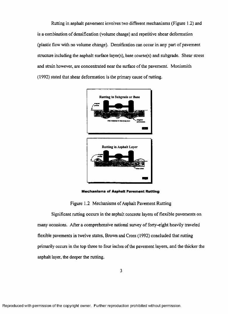
Rutting in asphalt pavement involves two different mechanisms (Figure 1.2) and
is a combination o f densification (volume change) and repetitive shear deformation
(plastic flow with no volume change). Densification can occur in any part o f pavement
structure including the asphalt surface layer(s), base course(s) and subgrade. Shear stress
and strain however, are concentrated near the surface of the pavement. Monismith
(1992) stated that shear deformation is the primary cause of rutting.
Rutting in Subgrade or Base
Rutting in Asphalt Layer
M echanism s of Asphalt Pavement Rutting
Figure 1.2 Mechanisms of Asphalt Pavement Rutting
Significant rutting occurs in the asphalt concrete layers o f flexible pavements on
many occasions. After a comprehensive national survey of forty-eight heavily traveled
flexible pavements in twelve states, Brown and Cross (1992) concluded that rutting
primarily occurs in the top three to four inches of the pavement layers, and the thicker the
asphalt layer, the deeper the rutting.
3
Reproduced with permission of the copyright owner. Further reproduction prohibited without permission.
Page 27
Hofstra and Klomp (1972) o f the Shell Laboratory in the Netherlands contradict
Brown and Cross (1992). After a study with a Laboratory Test Track (LTT, 3.25m in
diameter and 0.7m o f track width), they conclude that asphalt pavement rutting will be
significantly reduced with the increase in thickness o f asphalt concrete layer.
It has been generally agreed that rutting reduces road serviceability and causes
serious traffic safety problems. As wheel loads and tire pressures o f truck traffic on
highways have increased in recent years, rutting has become more serious. Many state
DOTs pay special attention to minimize rutting when designing and constructing asphalt
concrete pavements. The use o f large stone asphalt mixture is one way to reduce rut
susceptibility o f asphalt concrete.
1.1.2 Moisture Damage or Stripping in Asphalt Pavements
Stripping (often called moisture induced damage) is defined as the weakening or eventual
loss o f the adhesive bond between the aggregate surface and the asphalt cement in an
asphalt pavement or mixture in the presence o f moisture (water) (Roberts et al, 1994).
Although many factors contribute to the degradation of asphalt concrete pavements,
water is a key element in the deterioration of the asphalt mixture. According to Terrel
and Al-Swailmi (1994), there are three mechanisms by which water can degrade the
integrity o f an asphalt concrete matrix. These are: 1) loss o f cohesion (strength) and
stiffness o f the asphalt film due to several mechanisms; 2) failure o f the adhesion (bond)
between the aggregate and asphalt, and 3) degradation or fracture o f individual aggregate
particles when subjected to freezing. When the aggregate tends to have a preference for
absorbing water, the asphalt is “stripped” away (Figure 1.3). Stripping causes premature
pavement distress and ultimately the failure o f asphalt pavement.
4
Reproduced with permission of the copyright owner. Further reproduction prohibited without permission.
Page 28
Figure 1.3 Severe Stripping of a HMA Base Courses (from Roberts et al, 1994)
Stripping typically begins at the bottom of the HMA layer and progresses upward.
It is difficult to identify this distress without opening up the pavement structure because
the surface manifestations can take numerous forms such as excessive rutting, shoving,
corrugations, raveling, or cracking. In addition to improved asphalt binder adhesion
(such as with an anti-strip agent), appropriate mixture design and adequate drainage in
the pavement structure should be maintained in order to prevent stripping.
The use o f open-graded large stone asphalt mixtures provides positive drainage
system in newly designed highways or in reconstruction o f existing roadways. Using a
standard ASTM No. 57 size stone or large, it has been found that stability o f the drainage
layer can be maintained during construction while permitting enough air voids in the mix
to carry sufficient quantities o f water for drainage.
5
Reproduced with permission of the copyright owner. Further reproduction prohibited without permission.
Page 29
Louisiana currently uses an asphalt treated drainage blanket as a two inch (50.8-
mm) lift under Portland concrete pavements as specified in section 508 o f the standard
specifications (LaDOTD, 1998). A n evaluation of the first drainage blanket placed in
1977 indicated that while performing better than pavements without a drainage blanket,
the flow rate of water was much less than the design value and significantly less than the
flow rates suggested in the FHWA guidelines (FHWA, 1992). The Louisiana
specification uses a relatively small nominal size aggregate that produces air void system
that does not permit the prescribed flow rate. Currently, these drainage blankets are not
used in full depth asphalt concrete pavement design and no structural support is assigned
to this layer.
1.1.3 Proposed Louisiana Solution of LSAM
Louisiana has been experiencing rutting and moisture induced damage for many years.
With a hot and humid climate, the prevention of these distresses is among the top
priorities during the design and construction o f asphalt pavements. It has been proposed
that large stone asphalt mixtures (LSAM) be used for improved structural support of
asphalt pavements. Work by Ameri-Gaznon and Little (1990) indicates that the
maximum shear stress due to pavement loading occurs in a zone approximately two to
four inches deep in the pavement system. LSAM base courses should provide increased
strength in this zone of the pavement to resist rutting potential. Similarly, an open-graded
LSAM will provide excellent permeability and at the same time maintain or increase the
structural capacity
6
Reproduced with permission of the copyright owner. Further reproduction prohibited without permission.
Page 30
1.2 BACKGROUND AND LITERATURE REVIEW
1.2.1 Large Stone Asphalt Mixtures
Large stone asphalt mixtures (LSAM) are defined as HMA paving mixtures containing
maximum aggregate sizes between 25 and 63 mm (1 and 2.5 inch) (TTI, 1997). LSAM
may be dense-graded, stone-filled or open-graded. The philosophy o f using LSAM is to
use stone-on-stone contact o f the larger stones in order to minimize plastic deformation
under heavy traffic load.
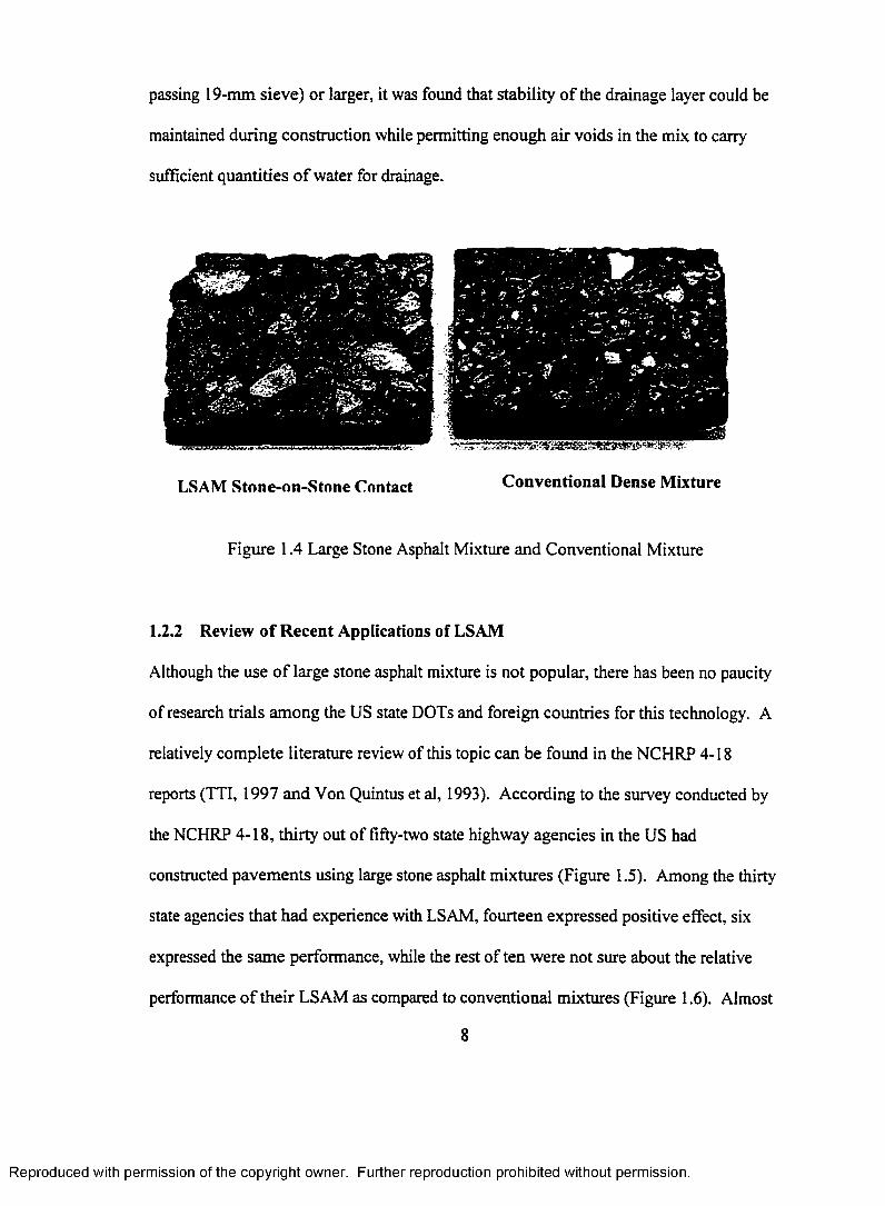
The concept of large stone asphalt mixture was introduced when the Warren
Brothers Company in May 1903 applied for and obtained a patent that employed large
size aggregates in asphalt mixtures (Khosla and Malpass, 1997). The principle of the
patent was that traffic loads would be mainly supported by the interlocking effect of the
larger aggregates, and that asphalt and smaller mineral aggregates would only provide
binding between bigger aggregates and to waterproof the mixture by filling up the voids
(Figure 1.4). Use o f the Warren Brothers product required paying royalties and as a
result, highway departments chose to specify with smaller top size aggregates to avoid
infringing on the patent. Such a practice (the use of small stone) has lasted up to this
date, largely due to the fact that smaller aggregates are easier to handle in automated
machine processing.
With the rapid increase o f traffic loads and volume, premature rutting has curred
more and more frequently in recent years. The concept o f stone-on-stone contact in large
stone asphalt mixtures seems to provide a solution for rut-resistant, durable heavy-duty
mixtures. Open-graded large stone asphalt mixtures were advocated in both concrete and
asphalt pavement for this purpose. Using a standard ASTM No. 57 size stone (80%
7
Reproduced with permission of the copyright owner. Further reproduction prohibited without permission.
Page 31
passing 19-mm sieve) or larger, it was found that stability o f the drainage layer could be
maintained during construction while permitting enough air voids in the mix to carry
sufficient quantities o f water for drainage.
LSAM Stone-on-Stone Contact Conventional Dense Mixture
Figure 1.4 Large Stone Asphalt Mixture and Conventional Mixture
1.2.2 Review of Recent Applications of LSAM
Although the use o f large stone asphalt mixture is not popular, there has been no paucity
of research trials among the US state DOTs and foreign countries for this technology. A
relatively complete literature review of this topic can be found in the NCHRP 4-18
reports (TTI, 1997 and Von Quintus et al, 1993). According to the survey conducted by
the NCHRP 4-18, thirty out o f fifty-two state highway agencies in the US had
constructed pavements using large stone asphalt mixtures (Figure 1.5). Among the thirty
state agencies that had experience with LSAM, fourteen expressed positive effect, six
expressed the same performance, while the rest of ten were not sure about the relative
performance o f their LSAM as compared to conventional mixtures (Figure 1.6). Almost
8
Reproduced with permission of the copyright owner. Further reproduction prohibited without permission.
Page 32
all the state agencies expressed the interest o f considering LSAM in the future (Table
1.1).
Number of LSAM Projects in 10 years
Figure l.5 Number o f LSAM Pavements Constructed Between 1987 and 1997
Poorer Same Better Unsure
LSAM Compared to Conventional Mix
Figure 1.6 Performance o f LSAM as Compared to Conventional Mixtures
9
Reproduced with permission of the copyright owner. Further reproduction prohibited without permission.
Page 33
Table l.l Responses from 52 Highway Specifying Agencies on LSAM (TTI, 1997)
Is your agency considering the use of LSAMs in the future?Yes: 41 agencies No: 1 agency No Response: 1 agency
(79%) (19%) (2%)Are you interested in knowing more about LSAM?
Yes: 50 agencies No: 1 agency No Response: I agency(96%) (2%) (2%)
Good performance in rut and fatigue crack resistance of dense-graded LSAM
compared with conventional mixture was reported in Kentucky (Anderson et al, 1991),
Minnesota (Acott et al, 1989), Nevada (TTI, 1997), North Carolina (Khosla and Malpass,
1997), Ohio (Abdulshafi et al, 1992), Tennessee, Texas, Wyoming, South Africa (TTI,
1994), Australia (Vail, 1993), and the former Soviet Union (Gorelyshev and Kononov,
1972). Anderson et al (1991) reported significantly better rut-resistance parameters with
LSAM than those with conventional mixtures on heavily trafficked pavements. They
also stated that LSAM with angular sands significantly reduced rut depth when compared
with mixes using rounded sand. Vail (1993) reported three LSAM trial projects
constructed in Australia and concluded that dense-graded LSAM increased both rut and
fatigue resistance.
Several sources reported that confined open-graded LSAM provided exceptional
rut-resistance. Good performance o f open-graded LSAM has been reported in Arkansas
(Von Quintus et al, 1993), Indiana (Fehsenfeld and Kriesch, 1988), Tennessee (Acott,
1988) and Wyoming (Von Quintus et al, 1993). Fehsenfeld and Kriesch (1988) reported
that, even though the LSAM base layers were highly permeable, no stripping was evident
and asphalt aging was minimal even after eight to eighteen years o f service. The NCHRP
10
Reproduced with permission of the copyright owner. Further reproduction prohibited without permission.
Page 34
4-18 report (TTI, 1997) attributed these properties to the relatively thick asphalt films in
LSAM.
It should be noted that while most o f the published literature reports good results
with LSAM; however, a DOT survey reported in NCHRP 4-18 (TTI, 1997) indicates that
the performance o f LSAM, particularly the dense-graded LSAM, are mixed. Some
LSAM have no rutting after the application o f very heavy traffic loads. Other pavement
structures containing LSAM experience premature rutting and do not show better
performance than the conventional mixtures. Coree et al (1997) reports findings from a
full-scale rutting test o f LSAM as part o f the NCHRP 4-18 study. By comparing the
rutting performance o f three different LSAM designs, they find that LSAM with poor
stone-on-stone contact exhibit the same high rut depths found in conventional binder
courses. Therefore, correct mix design is the key to ensure quality, rut-resistant LSAM.
1.2.3 Benefits of LSAM
Just as stated in the Warren Brothers’ patent, traffic loads are mainly supported by the
large size aggregates interlocking in the asphalt concrete. Coarse aggregate stone-on-
stone contact is the key that allows LSAM to outperform many conventional mixtures
(Figure 1.7). Many researchers (NAPA, 1988) found that asphalt concrete containing 25-
mm (1-inch) maximum size aggregates deformed less when subjected to shear load and
were denser and stronger than similar mixtures containing 19-mm (3/4-inch) maximum
aggregate. Van der Merwe et al (1989), based on South African experience, stated that
LSAM could improve both pavement structural capacity and save construction cost.
LSAM normally have lower voids in mineral aggregates (VMA) (TTI, 1994). In other
words, LSAM have higher relative volumes o f aggregates than conventional mixtures.
11
Reproduced with permission of the copyright owner. Further reproduction prohibited without permission.
Page 35
This characteristic results in higher densities, lower surface areas and lower optimum
asphalt contents of HMA mixtures. Lower asphalt content means lower material costs
compared to conventional mixtures (Khalifa and Herrin, 1970). The extensive use o f
coarser aggregates means less crushing energy is spent, which may lead to lower
aggregate cost. In addition, LSAM normally have thicker asphalt films than
conventional mixtures, which reduces the susceptibility to moisture damage and age
hardening (TTI, 1997).
Stone-on-Stone Contact
Figure 1.7 Stone-on-Stone Contact of LSAM
Khosla et al (1997) conducted a study on LSAM in North Carolina. In that study,
a 25-mm (1-inch) dense-graded LSAM binder mixture was compared with a conventional
North Carolina DOT H-Binder mixture through laboratory performance tests. They
concluded that their LSAM out-performed the conventional mixture in rut-resistance
while retaining similar fatigue crack resistance. Davis (1989) stated that the bearing
12
Reproduced with permission of the copyright owner. Further reproduction prohibited without permission.
Page 36
capacity o f a particular mix could be increased by more than four times when the top size
aggregate was changed from 19 to 37 mm (3/4 to 1.5 inch). It was pointed out that
LSAM were less sensitive to changes in asphalt cement properties, asphalt cement
content, and changes in temperature. Abdulshafi et al (1992) reported a two to three
times increase o f unconfined compressive strength and significantly lower creep and
much higher resilient modulus and fatigue resistance for LSAM when compared with
conventional mixtures.
1.2.4 Latest Development of LSAM Research
Most existing LSAM projects in the US were designed by the modified 152-mm (6-inch)
Marshall procedure developed by Kandhal (1990). This method produces a cylindrical
specimen o f 152-mm (6-inch) in diameter by 85-mm (3.4-inch) in height. It was
recommended for mixtures containing a nominal maximum aggregate size o f 37.5-mm
(1.5-inch). Kandhal increased the Marshall hammer mass and number o f blows to
achieve the same compaction energy per unit volume as in the conventional 102-mm (4-
inch) diameter by 63-mm (2.5-inch) high Marshall specimen. Although this procedure
was reasonably adequate for determining optimum asphalt content (Anderson et al.
1991), the Marshall mix design method is an empirical procedure that does not address
the fundamental engineering properties of asphalt mixtures and Marshall stability is not a
good indicator o f rutting potential. In addition, Kandhal (1990) reported that during the
compaction o f the 152-mm (6-inch) Marshall specimens, 75 to 112 blows per face of the
specimen often resulted in fracture o f the larger aggregates in the mixture.
According to the literature review conducted by the NCHRP 4-18 (TTI, 1997), the
Southern African Bitumen and Tar Association (SABITA) conducted a comprehensive
13
Reproduced with permission of the copyright owner. Further reproduction prohibited without permission.
Page 37
laboratory and field research program over several years, which resulted in an LSAM
design manual. The manual recognized that the strength and rut-resistance o f LSAM
were achieved from coarse aggregate interlocking. Durability was enhanced by thicker
asphalt films resulted from using large aggregate. To minimize stripping, the compacted
mixtures must either be impermeable or open-graded with interconnected voids so that
excessive pore water pressure cannot develop. Mixture designs that trap water should be
avoided. This design procedure recommended a 6-inch (150-mm) diameter, rotating-base
Marshall hammer with six depressions in the face that provided a certain kneading action.
Indirect tensile strength (ITS) and dynamic creep modulus were introduced for mix
characterization.
North Carolina Department o f Transportation and North Carolina State University
conducted a LSAM study during 1993 and 1997. In that study, they designed a dense-
graded LSAM with top aggregate size o f 25-mm (1-inch) based on modified Marshall
mix design method (Khosla and Malpass, 1997). The LSAM was compared with a
conventional North Carolina H-Binder mixture through laboratory indirect tensile
resilient modulus (Mr) tests, axial incremental creep tests, and indirect tensile fatigue
tests. The pavement analysis software, VESYS 3AM, was employed to predict
performance of the pavement test section on US Highway 70. They concluded that
LSAM pavement had lower permanent deformation than the conventional H-Binder
mixture under most test conditions. However, at high temperatures and long loading
times, the conventional mixture had slightly less permanent deformation than the LSAM.
The LSAM had a longer fatigue life than the conventional mixture, but only at initial
14
Reproduced with permission of the copyright owner. Further reproduction prohibited without permission.
Page 38
strain values o f greater than 5x1 O'4 mm/mm. At lower initial strain values, the
conventional mixture had a longer fatigue life.
The US Army Corps of Engineers conducted a study for the US Air Force to
analyzed the effects o f increasing the maximum aggregate size o f an asphalt mix from
19-mm to 25-mm in order to accommodate the increased tire pressure o f modem aircraft
(Regan, 1987). The study examined the tensile strength, direct shear, axial creep and
aging using different compaction methods and asphalt binders. The gyratory testing
machine (GTM) was used with pressures o f 0.7,1.4, 2.1 and 2.8 MPa. Their study
concluded that the 25-mm mixtures out-performed the 19-mm mixtures at higher
compaction efforts. The study also found that it was the asphalt binder type, instead of
top aggregate size, that most influenced the durability o f mixtures.
Perhaps the most comprehensive and recent study o f LSAM is Project NCHRP 4-
18, conducted by the Texas Transportation Institute (TTI, 1997). In that study, a
comprehensive literature review and survey o f 52 highway agencies about the status of
application as well as the performance o f LSAM was conducted. The survey found that,
while most highway agencies showed interests in applying LSAM in highway
construction, the actual experience o f design and construction o f LSAM had been very
limited. Among the constructed LSAM pavements, the performance had been mixed.
Some o f them (LSAM) exhibited exceptionally good rut-resistance, while the
performance o f others was similar to that o f conventional mixtures. The NCHRP 4-18
report attributed the poor performance to the inadequate mix design. In an effort to
overcome this shortcoming, the NCHRP 4-18 study developed a mixture design guide for
LSAM. The report recommended the use o f Superpave Gyratory Compactor (SGC) or
15
Reproduced with permission of the copyright owner. Further reproduction prohibited without permission.
Page 39
rolling wheel compaction (AASHTO PP3) during mix design. The six-inch (150-mm)
Marshall hammer should only be used when the other two compaction means are
unavailable. Stone-on-stone contact was ensured by keeping the voids in coarse
aggregates (VCA) above eighty to ninety percent. A number of mixture characterization
tests, such as uniaxial creep and Superpave repetitive shear at constant height (RSCH),
were recommended. Field projects were constructed as a part o f the study to validate the
laboratory results. The report concluded that when properly designed, LSAM would
perform better than conventional mixtures in rut-resistance (TTI, 1997).
1.2.5 Numerical Simulations of Pavement Structure
Burmister (1943) solved a two-layer linear elastic system problem for stress and strain
distribution under a surface load. He used the stress and displacement equations o f
elasticity for a three-dimensional problem in his solution by assuming the Poisson's ratio
to be either 0 or 0.5. Based on B minister's method, Acum and Fox (1951) presented
exact solutions for strength and deflection at the center-line o f three-layer systems. Later
a number o f computer programs such as BISAR and ELSYM5 were developed to
calculate stress and strain distribution in a pavement system based on a modified form of
the Burmister method.
Layered elastic analytical solutions provided a basis for pavement structural
design. However, they over-simplified the material behavior by assuming linear
elasticity. Huang (1967) and other researchers (Barksdale, 1967) reformulated the above
solutions by introducing viscoelastic models for the asphalt layers o f the system. This
improves the analytical procedure considerably. Later software such as VESYS and
16
Reproduced with permission of the copyright owner. Further reproduction prohibited without permission.
Page 40
MICH-PAVE widely adopted viscoelastic models for the asphalt concrete and linear or
nonlinear elastic models for the base course and subgrade materials (Kenis, 1977).
Viscoelasticity and nonlinear elasticity improved the layered elastic solution, but
they still failed to capture an important characteristic o f paving materials, the plastic
behavior under traffic loads. Yandell (1971) and Smith (1984) used elasto-plastic models
o f the pavement system and introduced a numerical procedure of Mechano-Lattice
Analysis (Smith, 1986). They applied the procedure for a number o f flexible pavement
analyses in the U.S., South Africa and Australia. Chan and other researchers applied
elasto-plastic theory for a finite element analysis o f a flexible pavement base course
rutting study in Nottingham, UK (Chan et al, 1989).
While most analytical methods assumed two dimensional axisymetrical conditions,
Zaghloul and White (1993) applied three dimensional finite element analyses and made
possible dynamic analyses to simulate real traffic loads. They used a visco-elastic model
for the asphalt concrete, an extended Drucker-Prager model for the granular base course
and the Cam Clay model for the clay subgrade soils. The three-dimensional finite
element analysis is performed using the commercial finite element software, ABAQUS.
Zaghloul and White's research improved the analytical procedure significantly, but
they failed to address one important aspect o f asphalt concrete, the visco plasticity. Seibi
and Sharma at the Pennsylvania State University (PSU) developed an elastic visco-plastic
constitutive relation for asphalt concrete under high rates of loading (Seibi, 1993). The
model adds the rate dependent characteristics to the traditional Drucker-Prager plastic
model.
17
Reproduced with permission of the copyright owner. Further reproduction prohibited without permission.
Page 41
1.3 LIMITATION OF EXISTING PROCEDURES
The literature review shows that most LSAM design procedures today still base mix
design on empirical procedures, such as the modified Marshall method. As in most
mixture design, there is little or no mixture performance analysis involved during the
design procedure. A few researchers conducted limited laboratory performance tests on
mixtures they studied and the results varied. The NCHRP Project 4-18 did an excellent
job in summarizing the status o f the application of LSAM and in introducing a
performance-based LSAM design procedure. However, at the time of the study, the
Superpave design and analysis procedure was in the development stage. For example,
though the Superpave gyratory compactor (SGC) was recommended to compact
laboratory specimens, the study actually used the Texas gyratory compactor, which uses a
different angle and pressure from the SGC. The types o f laboratory performance tests
conducted in that study were also limited. Noticeably, permeability, a very important
property o f open-graded LSAM, was not studied in any o f the previous research.
Although the North Carolina study conducted a limited structural analysis of LSAM
through VESYS 3 AM simulation, none of the other studies conducted numerical analyses
o f LSAM pavements to compare the structural performance o f LSAM to that of
conventional mixtures. None o f the previous research conducted comprehensive
laboratory performance studies on LSAM.
1.4 SIGNIFICANCE OF THIS RESEARCH
The research conducted in this study was designed to overcome the limitations of the
current procedures used to design and analyze LSAM. Table 1.2 lists a summary
comparison o f research elements for previous research studies and the research conducted
18
Reproduced with permission of the copyright owner. Further reproduction prohibited without permission.
Page 42
in this study. This research was aimed at establishing the fundamental engineering
properties o f LSAM for potential use in Louisiana. Superpave gyratory compactor
(SGC) was the standard compaction device used in this study. A dense-graded 37.5-mm
(1.5-inch) LSAM was designed according to the Superpave mix design protocol and was
intended to replace the Louisiana DOTD conventional Type 5A base mixture. An open-
graded LSAM was designed both to provide additional structural support and excellent
drainage for the pavement structure. The open-graded LSAM was recommended as a
replacement for the Louisiana DOTD conventional Type 508 drainable mixture.
The 3-D dynamic viscoplastic finite element analysis developed in this study was
able to predict the pavement responses under dynamic traffic loads.
Table 1.2 Comparisons of Research Elements for Previous Research and This Research
Research Elements NCHRP4-18
NorthCarolina WES South
AfricanThis
Research
Mix Design CompactionTexas
GyratoryCompactor
6-inchMarshall GTM
RollingMarshallHammer
SuperpaveGyratory
CompactorQuantify Stone-on-Stone
Contact Yes No No No Yes
Resilient Modulus (M r) Yes Yes No No YesAxial Creep Yes Yes Yes Yes Yes
Indirect Tensile Strength (ITS) Yes Yes Yes Yes Yes
Indirect Tensile Creep No No No No YesRepetitive Shear at
Constant Height (RSCH) Yes No No No Yes
Loaded Wheel Test (LWT) No No No No Yes
Moisture Susceptibility No No No No YesPermeability No No No No Yes
Structural Analysis No VESYS No No Yes (FE Simulation)
19
Reproduced with permission of the copyright owner. Further reproduction prohibited without permission.
Page 43
CHAPTER 2.OBJECTIVE AND SCOPE
2.1 OBJECTIVE
The objectives o f this study were as follows:
• Design two large stone asphalt mixtures (LSAM) as possible alternatives to the
conventional Louisiana DOTD Type 5A base mixture and Type 508 open-graded
drainable base mixture. The dense-graded large stone (37.5-mm) Superpave
mixture and an open-graded large stone asphalt mixture were designed to ensure
the stone-on-stone contact and other volumetric criteria are satisfied;
• Perform fundamental engineering property tests on the two LSAM mixtures and
the Louisiana DOTD conventional Type 5A base mixture and Type 508 drainable
base mixture;
• Develop test equipment and procedures to measure the permeability o f both open-
graded and dense-graded asphalt mixtures;
• Establish correlations between the volumetric properties and permeability o f the
asphalt mixtures included in this study;
• Develop a visco-plastic model that can be used to calculate the stress and strain
response o f asphalt mixtures in the pavement structures;
• Develop a three dimensional dynamic finite element procedure that can reflect the
dynamic responses o f asphalt pavement under the traffic loads;
• Conduct finite element analysis o f an existing pavement to validate the visco
plastic model developed;
20
Reproduced with permission of the copyright owner. Further reproduction prohibited without permission.
Page 44
• Conduct numerical simulation o f four pavements containing the two LSAM
designed in this study and two Louisiana conventional mixtures to evaluate the
added structural support of the LSAM mixtures.
2.2 SCOPE
The scope o f this study included the evaluation o f two large stone asphalt mixtures along
with their conventional Louisiana DOTD mixtures. The large stone asphalt mixtures
were open-graded and dense-graded, whereas, the conventional mixes were LaDOTD
Type 508 drainable base mix and Type 5A base mix. Each type of LSAM had three
types asphalt cement to study the effects o f binder on the performance o f large stone
asphalt mixtures. Table 2.1 presents the eight mixtures considered in this study.
Table 2.1 Eight Mixtures Designed in this StudyMix Type Mixture Symbol Aggregate Asphalt Cement
Open-gradedMixes
Type 508 Drainable Base Mix DT-P Limestone PG 70-22M
Open-graded LSAMOG-P Limestone PG 70-22M
OG-MG Limestone PG 70-22MA.ltOG-A Limestone PG 64-22
Dense-gradedMixes
Type 5 A Base Mix A-P Limestone PG 70-22M
Dense-graded LSAML-P Limestone PG 70-22M
L-MG Limestone PG 70-22MA.ltL-A Limestone PG 64-22
The laboratory performance of the mixtures was characterized through
fundamental engineering property tests. The engineering property tests conducted in this
study included:
• Indirect tensile resilient modulus at 4, 25 and 40 °C;
• Indirect tensile strength and strain at 25 °C;
• Axial creep at 40 °C;
• Indirect tensile creep at 40 °C;21
Reproduced with permission of the copyright owner. Further reproduction prohibited without permission.
Page 45
• Frequency sweep at constant height;
• Repetitive shear at constant height;
• APA rut at 60 °C;
• Permeability;
• Moisture susceptibility;
• Draindown.
In order to utilize the results from fundamental mixture characterization to predict
pavement performance, a 3-D dynamic finite element procedure was developed. In the
numerical analysis, a visco-plastic model was developed to describe the stress-strain
relationship of asphalt mixtures.
A test pavement section from the Louisiana Pavement Test Facilities (LPTF) was
selected to validate the material models and the finite element procedures. The numerical
simulation o f the Accelerated Loading Facility (ALF) test lane was compared to field
stress and strain measurement. After model validation, two comparable groups of
pavement structures, open-graded LSAM versus conventional Louisiana DOTD Type
508 drainable base and the 37.5-mm dense-graded LSAM versus conventional Louisiana
DOTD Type 5A base mixture, were analyzed for their responses to the similar dynamic
traffic loading.
22
Reproduced with permission of the copyright owner. Further reproduction prohibited without permission.
Page 46
CHAPTER 3.METHODOLOGY
This chapter describes the method and procedures applied in this study. The first part of
the section 3.1 describes the equipment and facilities used to conduct laboratory test and
numerical analysis of LSAM. The equipment includes specimen preparation facilities,
mixture performance test facilities, and the computing facility. Mix specimen
preparation facilities include two Superpave gyratory compactors. Mixture performance
test facilities include the MTS, Cox & Son 7000 Superpave Shear Tester, Cox & Son
Axial Testing System, Asphalt Pavement Analyzer, and LTRC Dual Mode Permeameter.
Section 3.2 presents the development o f test factorials o f the study. Section 3.3 describes
the materials (aggregates and asphalt binder) used in this study. Section 3.4 describes the
development o f mixture design o f the 37.5-mm (1.5-inch) Superpave LSAM and the
37.5-mm (1.5-inch) open-graded LSAM. Section 3.5 describes the mixture performance
test procedures.
3.1 FACILITIES
3.1.1 Specimen Preparation Facility
Asphalt mixture specimens were first mixed in a mixing bowl (Figure 3.1), mixing
bucket (Figure 3.2) or a mini-pugmill mixer (Figure 3.3). Two Superpave gyratory
compactors (SGC), a Pine Instrument Model AFGC125X (Figure 3.4) and a Troxler
Model 4140 (Figure 3.5), were used to compact the specimens.
The Superpave gyratory compactor (SGC) is a laboratory compaction device used
in the Superpave mix design system. The SGC mold is 150-mm in diameter The SGC
consists o f the following main components as shown in Figure 3.6:
• Reaction frame, rotating base, and motor;23
Reproduced with permission of the copyright owner. Further reproduction prohibited without permission.
Page 47
• Loading system, loading ram, and pressure gauge;
• Height measuring and recording system; and
• Mold and base plate.
Figure 3.1 Mixing Bowl
Figure 3.2 Mixing Bucket
24
Reproduced with permission of the copyright owner. Further reproduction prohibited without permission
Page 48
Figure 3.3 PH Double Pugmill Mixer
Figure 3.4 Pine Instrument Superpave Gyratory Compactor
Reproduced with permission of the copyright owner. Further reproduction prohibited without permission.
Page 49
Figure 3.5 Troxler Superpave Gyratory Compactor
height measurementcontrol and data
acquisition panel
loading ^ ram
reactionframe
rotatingbase
Figure 3.6 Components o f Superpave Gyratory Compactor (Asphalt Institute, 1994)
Figure 3.7 shows the configuration of a SGC mold, which has an inside diameter
o f 150 mm and a nominal height o f 250 mm. A base plate fits in the bottom o f the mold
to confine the specimen during compaction.
26
Reproduced with permission of the copyright owner. Further reproduction prohibited without permission.
Page 50
Figure 3.7 SGC Mold Configuration and Compaction Parameters
3.1.2 Mixture Performance Test Facility
Mixture performance testing includes loading and non-loading tests. Non-loading testing
in this study includes only the permeability test, which was performed in the dual-mode
permeameter developed during this study (described in detail in section 3.6). The loading
tests can be divided into: 1) axial loading; 2) diametrical loading; 3) shearing; and 4)
traffic simulating loading. Axial and diametrical loading tests were performed on the
Material Testing System (MTS) 810 and the Cox and Sons CS7500 Axial Testing and
Environmental System. Shearing tests were performed on the Cox and Sons CS7000
Superpave Shear Tester. An Asphalt Paving Analyzer was used to perform loaded wheel
rut testing.
3.1.2.1 Materials Testing System (MTS Model 810)
The LTRC’s Material Testing System (MTS Model 810, Figure 3.8) device is a closed-
loop controlled servo-hydraulic test system. The system is equipped with an
27
Reproduced with permission of the copyright owner. Further reproduction prohibited without permission.
Page 51
environmental chamber. The machine is rated 244 kN (55,000 pounds). Its state-of-the-
art digital controller, that is operated under Microsoft Windows NT4.0 and MTS Test
Star software, conducts the data acquisition and equipment control. Figure 3.9 shows a
schematic representation o f the test system. The closed-loop system consists o f a
computer and a digital controller acting as the controlling unit over a servo valve, a
hydraulic actuator, and the test specimen. The initial loading signal is sent from the
digital controller to the servo valve, which applied hydraulic pressure on the specimen,
from which the linear variable differential transformers (LVDTs) or the force sensors
return the feedback signal to the digital controller. The digital controller compares this
feedback signal with the control signal and performs adjustments as necessary.
Figure 3.8 Material Testing System (MTS 810)
28
Reproduced with permission of the copyright owner. Further reproduction prohibited without permission.
Page 52
Feedback S q m I
Diqittl C o n tro if
II the control signal is commanding a given force (sometimes referred to as "in force control"), the feedback signal is from the force sensor.
if iho control signal is commanding a given displacement, the feedback signal is from the LVDT.
IControl Signal
Lead Frame
Hytfaulic PressureHydraulic Actuator
Figure 3.9 Closed-loop Controlled Servo-hydraulic Test System
3.1.2.2 Cox and Son CS7500 Axial Testing System
The LTRC’s Cox and Sons CS7500 Axial Testing and Environmental System is a
versatile, fully automated, single axis, closed-loop hydraulic testing system specifically
designed to perform tests on soils and asphalt concrete mixtures over a wide range o f
stresses and frequencies. The equipment has sufficient flexibility to perform special or
standard tests.
The system software features custom test templates that automatically perform
SHRP and AASHTO tests, analyze the results and present the data in the report-ready
format.
The system software incorporates standard test and data acquisition templates to
perform tests that may be required for various research projects including the following
tests:
• Dynamic (sine, square and triangular wave);
29
Reproduced with permission of the copyright owner. Further reproduction prohibited without permission.
Page 53
• Creep;
• Repetitive loading (haversine);
• Constant rate (ramp);
• Fatigue;
• Random loading;
• Custom software templates for other tests are made available for tests
that fall within the static and dynamic capabilities o f the system.
Figure 3.10 Cox and Son CS7500 Axial Testing and Environmental System
3.1.2.3 Cox and Son CS7000 Superpave Shear Tester
The Superpave Shear Tester (SST) used in this study is a Cox and Sons Model CS7000
(Figure 3.11) manufactured by Cox and Sons, Inc. in Colfax, CA. The Superpave shear
test system is used to perform nearly all o f the load-related performance tests including:
volumetric test, uniaxial strain test, simple shear test at constant height, frequency sweep
30
Reproduced with permission of the copyright owner. Further reproduction prohibited without permission.
Page 54
test at constant height, repeated shear test at constant stress ratio, and repeated shear test
at constant height. The SST system includes the following components:
• loading device (load actuators o f hydraulic system);
• specimen deformation measurement equipment (testing apparatus);
• environmental chamber;
• control and data acquisition system.
The following table (Table 3.1) contains the minimum requirements o f the
system:
Table 3.1. Minimum SST System RequirementsM easurement Range Resolution Accuracy
Load 0-31000N 2 5 N
Confining Pressure 0-1000 KPa 0.5 KPa 1.0 KPa
Vertical or Axial Deformation (Constant Ht., Freq. Sweep
0-5 mm 0.0025 mm 0.005 mm
Horizontal Deformation (Freq. Sweep, Repetitive Shear)
0-0.050 mm 0.001 mm 0.002 mm
Radial Deformation 0-1 mm 0.005 m 0.010 mm
Temperature -10 to 80°C 0.25°C 0.5°C
Figure 3.11 CS7000 Superpave Shear Tester
31
Reproduced with permission of the copyright owner. Further reproduction prohibited without permission.
Page 55
3.1.2.4 Asphalt Pavement Analyzer
The Asphalt Pavement Analyzer (APA, Figure 3.12), is a multi-functional Loaded Wheel
Tester (LWT), used for evaluating the susceptibility to permanent deformation (rutting),
fatigue cracking, and moisture damage o f asphalt mixes. It features controllable wheel
load and contact pressure that are representative of actual field conditions. Triplicate
beam specimens, or six cylindrical (gyratory or roadway cores) specimens in three
specially designed specimen molds can be tested under controllable temperature and
under dry or submerged-in-water environments.
LTRC’s APA has the Automated Asphalt Pavement Analzer (AAPA) Software,
which allows the user to obtain rutting and fatigue measurements using a personal
computer to record and store data. The data acquisition system can take up to five
measurements during a single pass over a rectangular specimen and up to two
measurements during a single pass over a cylindrical specimen (vibratory, gyratory,
marshall specimens, or field cores). This information is stored on the PC and
subsequently used for data analysis. The results will not only include rutting at a specific
number of cycles but also allows the computation of the rate o f change o f deformation.
3.1.2.5 LTRC Dual Mode Permeameter
A dual mode permeameter (Figure 3-13) was developed in this study. The initial device
was purchased from the Virginia LAB Supply Corporation. Modifications were made to
the original device so that it can be used to measure hydraulic conductivity o f different
materials from dense-graded low permeable mixtures to open-graded drainable mixes
under both constant and falling head modes.
32
Reproduced with permission of the copyright owner. Further reproduction prohibited without permission.
Page 56
Figure 3.12 Asphalt Pavement Analyzer
Figure 3.13 LTRC Dual Mode Permeameter
The LTRC Dual mode permeameter consists o f a flexible wall cell, a top reservoir
tube, a bottom constant-head drainage tube, a flexible wall pump, two pressure
transducers and a data acquisition system (Figure 3.14). Two pressure transducers33
Reproduced with permission of the copyright owner. Further reproduction prohibited without permission.
Page 57
installed at the top and bottom of the specimen give accurate readings o f the hydraulic
head difference during the test. Data acquisition makes it possible to have continuous
readings during a falling head test so that the test can be conducted even at very high
flow rates (for drainable mixes). The specimen is placed in an aluminum cell with an
anti-scratch rubber membrane that is clamped tightly at both end of the cylindrical cell
into which the specimen is placed. A vacuum is applied between the membrane and the
cell to facilitate the installation of the specimen. During the test, a confining pressure o f
up to 103.5 kPa (15 psi) is applied between the membrane and the cell to prevent water
from short-circuiting around the perimeter o f the specimen. Two different top reservoir
tubes have been designed for different materials: a 25-mm (1-inch) diameter tube is used
for dense graded or less permeable materials and a 75-mm (3-inch) diameter tube is used
for highly permeable materials, both tubes are 90-mm (3-feet) long.
A vacuum is applied on the top of the reservoir tube before the test to saturate the
specimen.
Vito* VI
Figure 3.14 Diagram of LTRC Dual Mode Permeameter
34
Reproduced with permission of the copyright owner. Further reproduction prohibited without permission.
Page 58
3.1.3 Computational Facility
Numerical simulation using a finite element analysis was performed on a Sun
Microsystem Ultra 10 Workstation. The workstation is powered with a 333 MHz
UltraSPARC Hi CPU, which offers the numerical computation speed 14.1 SPECint95
and 18.3 SPECfp95 (One SPEC95 is defined as the speed o f a Sun SPARCstation 10/40
with 128 MB of memory). The following is a brief description o f the main features o f the
machine:
CPU: 333 MHz UltraSPARC Iii, 2MB cache;
RAM: 512 MB DIMM (50ns);
Storage: 10 GB SCSI HD, 32xCD, 8-mm Tape Backup;
Graphics: 24-bit on-board PGXx24, Creator3D graphics, 21” Display;
Network: 10/100BASE-T Ethernet;
OS: Sun Solaris 2.6.
The commercial finite element software, ABAQUS version 5.8 was installed on the Ultra
10 workstation.
3.2 MATERIALS
3.2.1 Asphalt Binder
Three types o f asphalt cement are included in this study: an SB polymer modified asphalt
cement meeting Louisiana Superpave performance grading specification o f PG 70-22M,
a conventional asphalt cement meeting Louisiana DOTD specification o f PG 64-22, and a
gelled asphalt cement meeting Louisiana DOTD Superpave performance grading
specification o f PG 70-22MAlt. One hundred percent crushed siliceous limestone will be
used for the design o f large stone asphalt mixtures as well as the laboratory samples of
35
Reproduced with permission of the copyright owner. Further reproduction prohibited without permission.
Page 59
conventional mixtures. Table 3.2 presents the asphalt cement properties and the
specifications o f the Louisiana Department o f Transportation and Development
(LaDOTD).
Table 3.2 LaDOTD Performance Graded Asphalt Cement Specification & Test Results
PropertyPG 70-22M PG 70-22M alt PG 64-22
Spec. TestResult Spec. Test
Result Spec. TestResult
Test on Original BinderRotational Viscosity
@ 135° C, Pa.s, TP 483.0 1.05 3.0- 2.85 3.0 0.463
Dynamic Shear, 10 rad/s, G*/Sin Delta,
kPa, TP 5
1.0+@64°C 3.7 1.0+@64°C 2.9l.0+@64°C 2.1
1.0+@70°C 2.0 l.0+@70°C 1.5
Flash Point, °C ,T 48 232+ 305 232+ 310 232+ 295Solubility, %, T 44 99.0+ 99.6 99.0+ 99.6 99.0+ 99.6
Softening Point, Ring & Ball, °C, T 53
N/A — 70.0+ 71.1 N/A —
Force Ductility, 4°C, 5 cm/min, 30 cm
elongation, kg, T 3000.234 0.35 N/A — N/A —
Tests on Rolling Thin Film Oven ResidueMass loss %, T 240 1.00- 0.10 1.00- 0.07 1.00- 0.03Dynamic Shear, 10 rad/s, G*/Sin Delta,
kPa,TP 5
2.20+@64°C 8.2 2.20+@64°C 7.52.20+@64
°C 4.22.20+@70°C 5.0 2.20+@70°C 3.1
Elastic Recovery, 25°C, 10cm
elongation, %, T 30140+ 85 N/A — 40+ 25*
Tests on Pressure Aging Vessel ResidueDynamic Shear, @
25°C, 10 rad/s, G* Sin Delta, kPa, TP 5
5000- 3175 5000- — 5000- 3628
Bending Beam Creep Stiffness, S, Mpa @ -
12°C, TP1300- 99 300- — 300- 238
Bending Beam Creep Slope, m value, @ -
12°C, TP10.300+ 0.452 0.300+ — 0.300+ 0.310
* Did not meet Elastic Recovery Criteria
36
Reproduced with permission of the copyright owner. Further reproduction prohibited without permission.
Page 60
3.2.2 Aggregates
The aggregates used in this study were siliceous limestone provided by the Vulcan
Materials Company from the Reed quarry in Kentucky. Table 3.3 presents the aggregate
gradations as provided by the supplier and the results of sieve analysis to verify the
gradations.
Table 3.3 Gradations from Stockpile Materials.
Sieve
No. 3 Vulcan Reed Limestone
No. 57 Vulcan Reed Limestone
No. 8 Vulcan Reed Limestone
Pass Spec Pass Spec Pass Spec(%) (% ) (% ) (%) (% ) (% )
63.5-mm(2.5”) 100 100 100 100 100 100
51-tnm (2”) 98.5 90-100 100 100 100 10037.5-mm
(1.5”) 60.6 50-80 100 100 100 100
25.4-mm (1”) 9.2 10-35 97.6 95-100 100 10019-mm (% ”) 2.7 0-10 77.7 80 100 100
12.7-mm (%”) 1.4 0-5 35.3 25-60 100 1009.5-mm(3/8”) 1.2 14.3 14 92.6 85-100
4.75-mm (No. 4) 1.0 1.9 0-10 25.1 10-30
-4.75-mm(-No.4) 0-10
Aggregate properties provided by the manufacturer are presented in Table 3.4. In
addition to the supplier provided data, flat and elongation test was performed for a
sample o f aggregates that has the same gradation as the designed mix (for aggregates that
are retained at No. 4 sieve and above). The test method is referred to ASTM D4791-95,
“Standard Test Method for Flat Particles, Elongated Particles, or Flat and Elongated
Particles in Coarse Aggregate,” (ASTM, 1998). It is found that 20.3% aggregates
exceeded the 1:3 criterion, whereas, 1.7% exceeded the 1:5 (Table 3.5).
37
Reproduced with permission of the copyright owner. Further reproduction prohibited without permission.
Page 61
Table 3.4 Aggregate Properties Provided by the ManufacturerAggregate Test Vulcan Reed Siliceous LimestoneProperties Protocols No. 3 No. 57 No. 8
B ulk (SSD) Spec. Gravity
ASTM C 127 2.69 2.688 2.661
Absorption ASTM C 127 0.4 0.2 0.3LA Abrasion ASTM C 131 22.0 21.5 21.0
Sulfate Soundness ASTM C 88 0.3 0.1 0.3Form ation Fort Payne Fort Payne Fort Payne
Unit W t. (lb/ft3)
Loose ASTM C 29 85.5 85.3 85.0Rodded ASTM C 29 100.0 96.7 97.0
Table 3.5 Results from the Flat and Elongation TestRatio Pass Flat Elongated Flat & Elongated
% % % %1:3 79.7 3.9 16.4 20.31:5 98.3 0 0 1.7
3.3 DEVELOPM ENT O F M IXTURE DESIGN
An asphalt mixture design is an optimization procedure that determines the optimum
aggregate gradation and asphalt content for compaction efforts. Table 3.6 presents the
job mix formulae for the four types o f mixtures designed in this study. Specific details of
section o f mixture gradations, measurement o f specific gravity o f large stone asphalt
mixtures, determination o f degree of stone-on-stone contact, as well as volumetric design
procedure for each individual mixtures are discussed in the following sections.
3.3.1 M ixture G radations
Mixture gradations determine the aggregate proportions o f different sieve sizes. Proper
aggregate gradations ensure robust aggregate skeletons in HMA mixtures. For large
stone asphalt mixture, NCHRP 4-18 (TTI, 1994) report suggests to select gradations
should always ensure adequate stone-on-stone contact.
38
Reproduced with permission of the copyright owner. Further reproduction prohibited without permission.
Page 62
Table 3.6 Job Mix Formulae
JobMix
Formula
Mix OG-LSAM Type 508 Sup-LSAM Type 5AAC% 2.5% 2.3% 3.8% 3.5%
Aggregates70%#3LS
100%#57LS
60%#3LS 37%#5LS 11%#78LS 21%# 11LS 12%CS 19%RAP*
13%#57LS 20%#57LS10%#8LS 3%HL
7%CS 7%DF
Gradation%Passing
63.5 mm (2.5”) 100 100 100 10050.8 mm (2”) 1001 100 1002 100
37.5-mm (1.5”) 79 100 86 10025-mm (1”) 43.7 98 65.24 96
19 mm (3/4”) 30.9 78 52.4 8412.5 mm (1/2”) 23.0 35 34.1 699.5 mm (3/8”) 18.3 14 25.8 61
No. 4 9.4 4 21.92 46No. 10 6.6 2 20 30No. 40 3.2 15.6 19No. 80 0.4 7.2 8
No. 200 0.1 5.4 5.3Gmb 1.915 1.760 2.459 2.410Gmm 2.592 2.584 2.546 2.507
VMA 30.7 36.0 11.7 12.3VFA 14.9 10.8 70.9 67.5
Air Voids 26.2 32.1 3.5 4.0Film
Thickness30.2 38.9 7.3 7.07
%Gmm@Njni 84.5%Gmm@Nfin 97.7
Note: LS - Limestone; CS - Coarse Sand; HL - Hydrated Lime; DF - Donna Fill.1 For lab mixtures, aggregates passed 50.1 mm (2 inch) were scalped.2 Mixtures would be 96.5% passing this sieve size for OG-LSAM;3 For Mixtures would be 98% passing this sieve size for Sup-LSAM;4 The GSb used for calculation was 2.68* Field design used RAP. Lab mixes used existing LS to match the gradation.
In order to use the existing laboratory compacting equipment, an aggregate top
size o f 37.5-mm (1.5-inch) was selected for both open-graded and dense-graded LSAM.
Several gradations were examined in order to ensure that volumetric criteria and stone-
on-stone contact was satisfied. It was a trial-and-error procedure. During the trial-and-
Reproduced with permission of the copyright owner. Further reproduction prohibited without permission.
Page 63
error process, mixes with different gradations were examined for their volumetric
properties and axial creep characteristics. For the open-graded LSAM, permeability was
also considered for the section o f gradation and optimum asphalt content.
Aggregate gradations for the conventional mixtures (Type 508 drainable base mix
and Type 5A base mix) were adopted from the current Louisiana DOTD specification
(LADOTD, 1992.)
Figure 3.15 shows all four gradations together in a semi-log scale and Figures
3.16 and 3.17 show the gradations in 0.45 power chart.
It is noticeable that the gradation o f Superpave LSAM (Sup-LSAM) goes through
the “Restricted Zone” in the Superpave 37.5-mm gradation chart (Figure 3.15). The
NCHRP 4-18 Report (TTI, 1997) suggested that the concept o f “Restricted Zone” should
not apply to LSAM mixtures due to their relatively coarse nature.
100
80
g 60o c*5n£ 40
20
00.01 0.1 1 10 100
Sieve Opening (mm)
Figure 3.15 Gradation Chart o f Four Mixtures in this Study
40
-♦-O G -LSA M -O -T y p e 508 -* -D en se -L S A M ;! -A -T y p e 5A T
Reproduced with permission of the copyright owner. Further reproduction prohibited without permission.
Page 64
O o
a>
£ oO CM
oo
oo © ©<0
o o« oCM
o© oo
Biassed ;uaoJ9d
41
Reproduced with permission of the copyright owner. Further reproduction prohibited without permission.
Figu
re
3.16
Gra
datio
n Ch
art
of La
rge
Ston
e A
spha
lt M
ixtu
res
Page 65
M£ y
o
<>
10
S °(A m
a o
o o ooo o
CAON55o>555
73<uu,3Xiuc/}eaCQ<<DaE-*
ooouaHCmOtsca-cUcoCQ■o2Or"rn2300
Buissed jueaied
42
Reproduced with permission of the copyright owner. Further reproduction prohibited without permission.
Page 66
3.3.2 LSAM Bulk Specific Gravity Test
The test to determine the bulk specific gravity Gmb is normally performed by placing
the mix samples into water and comparing the submerged weight and SSD weight
(ASTM D2726, AASHTO T166). But when the specimens contain open or
interconnecting voids, or absorb more than 2 % water by volume, the SSD method will
not provide an accurate measurement o f the bulk specific gravity. There are three
alternatives to overcome this problem: 1) put a rubber membrane around the specimen
before submerging; 2) coat the specimen with paraffin before submerging (ASTM
D 1188-89); or 3) replace the water with glass beads and perform the test as in the
AASHTO T166 or ASTM D2726. The NCHRP 4-18 proposed using glass beads for
the large stone asphalt mixture (TO , 1997). In this study, 8-mm glass beads were
used to determine the bulk specific gravity o f both the open-graded large stone asphalt
mixtures (OG_LSAM) and the conventional Type 508 drainable mixture.
Figure 3.18 shows the test set-up for measuring bulk specific gravity o f water
permeable, compacted HMA mixes using glass beads. Test equipment includes a half
cubic foot aluminum bucket (unit measure) and a metal cone that is intimately fitted to
the top o f the unit weight measure to form a large metal pycnometer. The cone must
be capable of being securely fastened to the unit weight measure and the cone must
attain the same relative position with the unit weight measure each time it is set in
position in order to ensure a constant volume for the pycnometer. Using the
recommendation of NCHRP 4-18 (TO , 1997), 8-mm glass beads were used.
43
Reproduced with permission of the copyright owner. Further reproduction prohibited without permission.
Page 67
The test procedure for measuring the bulk specific gravity o f a compacted
asphalt specimen using glass beads is as following:
• Record weight of asphalt specimen in air;
• Place 50.8 - 76 mm (2 to 3 inch) of beads in the bottom of the measure;
• Place specimen in the center o f the measure and resting on the beads; twist
the specimen to seat it in the beads;
• Fill the measure with beads to the top o f the specimen. Tap the measure
with the rubber mallet at four locations equally spaced around the
circumference with five blows per location;
• Fill the measure to overflowing with beads and tap the measure with the
rubber mallet at four locations equally spaced around the circumference
with five blows per location. Level the glass beads to the top of the
measure;
• Record the weight o f the measure plus cone plus beads plus specimen;
• Using the following equation (Eq. 3.1), calculate the bulk specific gravity
of the compacted asphalt specimen:
W G _______________ specimen beads______________ .>m h ~ W + W - W ' ’ 1
specimen measure+beads specimen+beaUs+measure+cane
where
Gmb = Bulk Specific gravity of asphalt specimen,
Gbeads = Bulk specific gravity of beads,
Wjpecimen = Weight o f specimen in air,
44
Reproduced with permission of the copyright owner. Further reproduction prohibited without permission.
Page 68
Wjneasure+beads= Weight of measure plus beads, and
Wspecimen+beads+measure+cone= Weight o f specimen+beads+measure+cone.
The air voids in the compacted specimen is calculated using the following
equation (Eq. 3.2):
V T M = 1 - GG .mm /
xlOO (3.2)
where
VTM = Percent air voids in the specimen,
Gmb = Bulk specific gravity o f the specimen, and
Gmm = Maximum (Rice) specific gravity o f specimen.
Figure 3.18 Unit Weight Measure, Cone, Glass Beads, and Specimen
Reproduced with permission of the copyright owner. Further reproduction prohibited without permission.
Page 69
3.3.3 Open-Graded LSAM Design
Open-graded LSAMs are commonly used for rapid drainage o f subsurface water.
These mixes contain a small amount o f fine aggregate (Table 3.6). When designing
the open-graded LSAM (OG_LSAM), it is desirable that mixture should have high air
voids, high voids in mineral aggregates (VMA) and sufficient asphalt cement for
durability. The angularity o f the coarse aggregate in these mixes provides the
interlock among particles. The asphalt content typically ranges from 1.5 - 2.5 percent.
The film thickness in these mixes generally significantly higher than conventional
dense-graded mixes. To prevent runoff of asphalt cement during transportation to the
job site, a lower mixing temperature is generally adopted. For each mixture design
included in this study, nine sets o f specimens (three asphalt content levels and three
SGC gyrations) were prepared and tested for their volumetric properties in order to
provide data for selecting the optimum design. Table 3.7 presents the air voids, VMA,
VFA at different asphalt contents and compaction levels. Figure 3.19 presents the
variation o f air voids with asphalt content and SGC compaction efforts. Figures 3.20a
and 3.20b show the relationship between VMA, VFA and the asphalt content and SGC
gyrations. It appeared that 2.5 percent of asphalt and 25 SGC gyrations produced the
optimum volumetric design for the open-graded LSAM.
3 .3.4 Superpave LSAM Design
The design o f this mixture was conducted according to AASHTO TP4 (1997). The
Nini, Ndes and Nmax were 8-, 100-, and 160-gyrations. The optimum asphalt content for
this mix was 3.8. The optimum volumetric design satisfied a Superpave 37.5-mm
46
Reproduced with permission of the copyright owner. Further reproduction prohibited without permission.
Page 70
(1.5-inch) mixture. Table 3.8 presents the volumetric properties o f the four mixes
used in this study.
Table 3.7 Volumetric Properties o f Open-graded LSAM at Different Asphalt ContentsAsphalt
Content (%)SGC
Gyrations A ir Voids VMA VFA Permeability K’ (mm/sec)
2.010 26.7 32.4 18.4 5.2525 22.4 28.2 20.8 5.0140 19 25.2 24.6 3.89
2.510 26 30.6 15.1 6.2525 26.2 30.7 14.9 7.1940 20.6 25.5 19.3 0.935
3.010 13.7 19.3 35.3 7.1925 11.8 17.5 33 0.43740 15.8 21.3 25.8 0.174
Note: K’ is the pseudo coe section 3.6.
Ticient o f permeability. Details of K’ are described in
Air Void vs AC Content (OG-LSAM)
20
10 10 SCC Oynoora
23 SGC OyraOons
40 SGC QyrM ora
25 AC %
Air Void vs SG C G yrations (OG-LSAM)
GL....0
20% AC
— • - 25% AC
— • 3 0% AC
Figure 3.19 Open-graded LSAM Air Voids
47
Reproduced with permission of the copyright owner. Further reproduction prohibited without permission.
Page 71
VMA vs AC Content (OG-LSAM.) VMA vs SGC Gyrations (OG-LSAM)
l*g*nd
to SGC Gyndorw
29 SCC Gyrafwna
40 SCC Cyrabona G -
20
Figure 3.20a Open-graded LSAM VMA
VFA vs AC Content (OG-LSAM) VFA vs SGC Gyrations (OG-LSAM)
O -
Figure 3.20b Open-graded LSAM VFA
48
Reproduced with permission of the copyright owner. Further reproduction prohibited without permission.
Page 72
Table 3.8 Volumetric Properties o f MixturesType508
OGLSAM Type 5A Sup
LSAMSuperpave Spec
(37.5-mm, Level II)AC% 2.3 2.5 3.5 3.8
Ndes (SGC) 25 25 100 100 100Gmm 2.584 2.592 2.507 2.546
Gmb (average) 1.760 1.915 2.410 2.459Air voids (%) 32.1 26.2 4.0 3.5 3 - 5
VMA (%) 36.0 30.7 12.3 11.7 >11.0VFA (%) 10.8 14.9 67.5 70.9 65 - 78*
Film Thickness (micron) 38.9 30.2 7.07 7.3
* Louisiana Modified Speci: 'ication (LADOTD, 1992)
3.3.5 Conventional Louisiana Type 5A and Type 508 Mix Design
These designs were selected from field projects. The optimum asphalt content for the
Type 5A base mix was determined from a standard Marshall mix design. A Louisiana
DOTD method specification (LADOTD, 1992) was used to determine the asphalt
content of the Type 508 mix.
3.3.6 Degree of Stone-on-Stone Contact
The stone-on-stone contact was determined based on the test procedure proposed by
NCHRP 4-18 (TTI, 1997). According to the procedure, the dry density of coarse
aggregate (above 4.75 mm or No. 4 sieve) was first determined through rodded weight
of the aggregates in a 0.028-m3 (1 cubic foot) container. The voids in coarse
aggregate can be calculated through the following equation:
\ G c a - d w) - D aV C A - 100 (3.3)
where
VC A is the voids content o f the coarse aggregate;
49
Reproduced with permission of the copyright owner. Further reproduction prohibited without permission.
Page 73
Gca is the specific gravity o f coarse aggregate;
dw is the density o f water; and
Dca is the density o f the coarse aggregate.
Stone-on-stone contact is defined as the ratio of the density o f the coarse
aggregate in the compacted LSAM to the density of coarse aggregate. The density of
the coarse aggregate in the compacted LSAM is calculated by the following equation:
D c m = { . G nib- d w) - { \ - A C y R (3.4)
where
Dcm is the density o f the coarse aggregate in the compacted LSAM;
Gmb is the bulk specific gravity of the compacted LSAM;
dw is the density o f water;
AC is the asphalt content as a weight percent o f the total LSAM;
R is the percent o f coarse aggregate in LSAM gradation retained
on 12.5 mm (0.5 inch) sieve for nominal maximum aggregate
size from 25 to 38 mm or on the 19 mm (3/4 inch) sieve for
nominal max. aggregate size from 38 to 64 mm.
The degree o f stone on stone contact is expressed by the following equation:
S S C = 100 (3.5)
where
SSC is the degree o f stone-on-stone contact in the compacted LSAM;
Dcm is the density o f the coarse LSAM; and
50
Reproduced with permission of the copyright owner. Further reproduction prohibited without permission.
Page 74
Dca is the density o f the coarse aggregate.
Table 3.9 presents the results of the voids in coarse aggregates and the degree
of stone-on-stone contact. It is shown that there is a 92 percent stone-on-stone contact
for the open-graded large stone asphalt mixture whereas for the 37.5-mm Superpave
mixture, there is an 85 percent o f stone-on-stone contact. The NCHRP 4-18
recommended eighty percent or more in LSAM for degree o f stone-on-stone contact.
Figure 3.21 presents a visual observation of stone-on-stone contact from the cut
mixtures.
Table 3.9 VCA and Degree o f Stone-on-Stone ContactMix Type Coarse Aggregate
Unit Density (g/cm3)
Coarse Aggregate Unit Density in LSAM
(g/cm3)
VCA SSC(%)
OG-LSAM 1.476 1.364 44.9 92Sup-LSAM 1.576 1.343 41.2 85
37.5 mm Superpave LS Opdi. GTradedCl' .. V .-»-A tr'TVTi.
Figure 3.21 Cut-Section Showing Stone-on-Stone Contact
51
Reproduced with permission of the copyright owner. Further reproduction prohibited without permission.
Page 75
3.4 DEVELOPMENT OF TEST FACTORIALS
Indirect tensile resilient modulus (M r) test, indirect tensile strength (ITS) and strain
test, axial creep test, indirect tensile creep test, Superpave simple shear frequency
sweep (FSCH) test, Superpave simple shear repetitive shear at constant height
(RSCH), Asphalt Pavement Analyzer (APA) rut test, and moisture susceptibility test
were performed to characterize the four mixtures in this study. In addition, a
permeability test was performed on the open-graded LSAM and the conventional
Louisiana Type 508 drainable mixtures. The specimens were prepared for each
mixture combination. Table 3.10 lists the performance tests proposed in this study and
the corresponding number of specimens tested.
Table 3.10 Mixture Performance Tests
Tests ProtocolsEngineeringProperties
MixturesOG
LSAMType508
SupLSAM
Type5A
Mr (5°C, 25°C, 40°C)
ASTM D 4123 (modified)
Elastic Properties (M R and p)
3x3 ‘ 3 3x3 3
ITS at 25 °C AASHTO T245 Durability and Fatigue Crack
3x3 3 3x3 j
Axial Creep at 40 °C
Tex-231-F(Tx DOT 1993)
PermanentDeformation
3x3 3 3x3 3
IT Creep at 40 °C
Mohammad et al (1993)
PermanentDeformation
3x3 3 3x3 3
RSCH at 60 °C
AASHTO TP7 Permanent Strain (Rut Susceptibility)
3x3 3 3x3 3
FSCH at 60 °C
AASHTO TP7 G*, 5 (Viscoelastic Properties)
3x3 3 3x3 3
APA Rut at 60°C
Georgia Spec. GDOT (1986)
Rut Susceptibility 3x3 3 3x3 3
DraindownTest
ASTM D 6390- 99
DraindownSusceptibility
3x3 3 0 0
Permeability Huang et al. (1999)
Coefficient o f Permeability
3 3 3 3
Lottman Test AASHTO TP283 Moisture Susceptibility 2x3x3 2x3x3 2x3x3 2x31 The number o f specimens needed to conduct the test (Tota number = 252)
52
Reproduced with permission of the copyright owner. Further reproduction prohibited without permission.
Page 76
3.5 MIXTURE PERFORMANCE CHARACTERIZATION
3.5.1 Specimen Preparation
Cylindrical specimens were fabricated for fundamental engineering property tests in
this study. The specimens were compacted in the Superpave Gyratory Compactors
(SGC, Figure 3.4 and 3.5) to a diameter of 150-mm (5.9-inch) and heights o f between
120-mm (4.7-inch) to 150-mm (5.9-inch). Samples for SST tests were cut to a height
o f 75-mm (3.0-inch). The specimens for APA rut test were cut into a height between
70-mm and 75-mm. The specimens were then placed into the APA cylindrical mold
and flushed with the top o f the mold using plaster o f Paris (Figure 3.22).
Figure 3.22 APA Rut Test Cylindrical Samples and Mold
53
Reproduced with permission of the copyright owner. Further reproduction prohibited without permission.
Page 77
3.5.2 Indirect Tensile Resilient Modulus (Mr) Test
The testing temperatures were 5,25, and 40 °C, and the test was conducted according
to the modified ASTM D 4123 (Mohammad et al, 1993). This test is a repeated load
indirect tension test for determining the resilient modulus o f the asphalt mixtures. The
recoverable vertical deformation SV and horizontal deformation 8H were used to
calculate the indirect tensile resilient modulus, M r and Poisson’s ratio, p according to
Equations (3.6) and (3.7):
= PiM + 0 2 7 )* t - S H ( T )
^ = 3 5 9 ^ 0 - 0 . 2 7 (3.7)S V { T )
where, M r - Resilient Modulus, MPa,
P - applied vertical load, N,
/ - sample thickness, mm,
p. - poisson’s ratio
S H ( T ) - horizontal deformation at time T , mm.
S V ( T ) - vertical deformation at time T , mm.
In order to successfully conduct the indirect tensile resilient modulus test, the
loading strip needs to be exactly centered. Even slight deviation will cause significant
errors for the test results. During this study, an indirect tensile loading frame was
fabricated to conduct various tests in the indirect tensile mode. Figure 3.23 shows the
test configuration of indirect tensile resilient modulus test and Figure 3.24 presents the
typical results from a M r test.
54
Reproduced with permission of the copyright owner. Further reproduction prohibited without permission.
Page 78
Figure 3.23 Test Setup o f Indirect Tensile Resilient Modulus (M r) Test
Reproduced with permission of the copyright owner. Further reproduction prohibited without permission.
Page 79
400
100 —
100 —
0.0 O.fi 1.0 3.0Dm* (itcond)
0.0013
r8S18 0.0004 -
10000
100 1.10 110 100
Figure 3.24 Typical IT Resilient Modulus (Mr) Test Results
56
Reproduced with permission of the copyright owner. Further reproduction prohibited without permission.
Page 80
3.5.3 Indirect Tensile Strength (ITS) and Strain Test
The indirect tensile strength (ITS) and strain test was used to determine the tensile
strength and strain o f the mixtures. This test was incorporated in the study to ensure
the durability of the mixtures would not be compromised while the rut resistance of
the mixtures was improved. This test was conducted at 25 °C according to AASHTO
T245. Each test specimen was loaded to failure at a 50.8 mm/min (2 inch/min)
deformation rate. The load and deformations were continuously recorded and indirect
tensile strength and strain were computed as follows:
St - Tensile strength, kPa
P„it - Peak load, N
t - Thickness o f the specimen, mm
D - Diameter o f the specimen, mm
Et - Horizontal tensile strain at peak load, and
Hr - Horizontal deformation at peak load.
Toughness index (TI), a parameter describing the toughening characteristics in
the post-peak region, was also calculated from the indirect tensile test results. Figure
3.25 presents a typical normalized indirect tensile stress and strain curve. A
dimensionless indirect tensile toughness index, TI is defined as follows:
(3.8)
e T = 0.0205 H r (3.9)
where
57
Reproduced with permission of the copyright owner. Further reproduction prohibited without permission.
Page 81
where
TI - Toughness index,
Ae - Area under the normalized stress-strain curve up to strain s,
Ap - Area under the normalized stress-strain curve up to strain sp
e - Strain at the point o f interest, and
£p - Strain corresponding to the peak stress.
0.8
T3a>N 0.6RJEWOW 0.4 I-
0.2
0.02.0 2.50.0 0.5 1.0 1.5 3.0 3.5 4.0
Strain %
Figure 3.25 A Typical Normalized ITS Curve for TI Calculation
58
Reproduced with permission of the copyright owner. Further reproduction prohibited without permission.
Page 82
This toughness index compares the performance of a specimen with that o f an
elastic perfectly plastic reference material, for which the TI remains a constant o f one.
For an ideal brittle material with no post-peak load carrying capacity, the value o f TI
equals zero. Similar analyses were reported by Sobhan, et al (1999). In this study, the
values o f indirect tensile toughness index were calculated at a tensile strain o f three
percent.
3.5.4 Axial Creep Test
This test was conducted in accordance with the Test Method Tex-231-F (Texas DOT,
1993). The test was conducted in an axial loading mode as shown in Figure 3.26. A
static load o f 1.220 kN (274 Ibf) was applied for the duration of one hour along the
centric longitudinal axis of the specimen (150-mm in diameter). The axial
deformation o f the specimen was continuously measured and subsequently used to
calculate creep properties such as stiffness, slope, and permanent strain. These data
were used to evaluate the permanent deformation characteristics o f asphalt mixtures.
The samples were tested at 40°C. A typical axial creep test result is illustrated in
Figure 3.27. The slope and strains are shown in the figure and the creep stiffness is
calculated as the compressive stress divided by the total strain at the end of the loading
period.
Higher stiffness, lower creep slope and lower permanent strain are desired for
rut-resistant mixtures. Texas specification (Texas DOT, 1993) specifies that a
minimum stiffness of 41.4 MPa, maximum creep slope of 3.5x10⁻⁸ and maximum
permanent strain value of 5x10⁻⁴ mm/mm for a satisfactory surface mixture.
59
Reproduced with permission of the copyright owner. Further reproduction prohibited without permission.
Page 83
Figure 3.26 Test Setup of Axial Creep Test
60
Reproduced with permission of the copyright owner. Further reproduction prohibited without permission.
Page 84
ISO600 secondsGO seconds
-»125
3600 seconds
100
E3&•os
0 1000 2000 2 0 0 0 4 0 0 0 5 000
time (second)
0 .0 0 6 — |
slope
■Cocc .t'i
TO
0 . 0 0 4 —
0 . 0 0 2 —
0.000 1 I 1 I 1 I r
1000 2000 2000
time (second)
4000 5000
Figure 3.27 Typical Axial Creep Test Results
61
Reproduced with permission of the copyright owner. Further reproduction prohibited without permission.
16
Page 85
3.5.5 Indirect Tensile Creep Test
This test is performed in the indirect tensile mode with a setup similar to that for the
indirect tensile resilient modulus (M r) and the indirect tensile strength (ITS) test
(Figure 3.23). At a testing temperature o f 40°C (104°F), a compressive load o f 1112.5
N (250 lbf) was applied to the specimen using the stress-controlled mode of the MTS
test system. The load was applied for 60 minutes or until specimen failure occurs
(Mohammad et al, 1993). The deformations acquired during this time were used to
compute the creep modulus as follows:
3 5 9 PS ( T ) = — —- (3.11)
t - 5 V { T )
where, S (T ) - creep modulus at time T , MPa,
P - applied vertical load, N,
t - specimen thickness, mm, and
5 V (T ) - vertical deformation at time T , mm.
Figure 3.28 shows the typical results of the load versus time, vertical
deformation versus time and creep stiffness versus time graph on a log-log scale for
the indirect tensile creep test. From this graph the creep slope was computed and used
in the analysis.
3.5.6 APA Rut Test
The Asphalt Pavement Analyzer (APA, Figure 3.12) is an enhanced version o f the
Georgia loaded wheel tester. The APA is capable of evaluating rutting, moisture and
fatigue cracking susceptibility o f asphalt concrete mixes. Loads, pressure and
62
Reproduced with permission of the copyright owner. Further reproduction prohibited without permission.
Page 86
MOO on n n d c-ocaoama
y —
yUmB (waond)
cco
uu? -
i«
u1m» (cvoond)
19aaa£ 'UUJJU - *aaea
ylimp (aaond)
Figure 3.28 Typical Results from Indirect Tensile Creep Test
63
Reproduced with permission of the copyright owner. Further reproduction prohibited without permission.
Page 87
temperature are adjustable, and dry or submerged test conditions can be selected. Test
temperature can be adjusted and maintained from 30°C to 65°C (85°F to 148°F) during
testing.
The APA can test three samples simultaneously (Figure 3.29). The concave
shaped wheels travel back and forth over a stiff, pressurized rubber hose that rests
directly on the specimen. A specimen slab is approximately 127 mm wide, 76 mm
deep and 320 mm long. Specimens can also consist o f 150 mm diameter field cores or
Superpave gyratory compacted specimens. In this study, 150-mm diameter laboratory
compacted cylindrical specimens were used in this test. Typical test conditions as set
by the Georgia DOT specification are at temperature of 40°C, 444.4 N load, and 0.7
MPa hose pressure with a failure criterion o f no more than 7.6 mm rut depth after
8,000 cycles (16,000 passes) under dry conditions. The wheel speed is approximately
60 cm/sec. In this study, a test temperature o f 60 °C was selected based on the
LTPPBIND database for the temperature o f the pavement at a depth o f 50-mm
(FHWA, 1999). LTPPBIND is a software developed by the FHWA Tumer-Fairbank
Highway Research Center for Determining Superpave Performance Grades Based on
LTPP and SHRP Pavement Temperature Models and Data from 7928 Weather
Stations in North America.
The LTRC’s APA is capable o f recording rut depth automatically. Average rut
depth vs. number o f load cycles, slope o f rut depth vs. number o f load cycles, and
change o f slopes vs. number o f load cycles, can be drawn to analyze the rutting
64
Reproduced with permission of the copyright owner. Further reproduction prohibited without permission.
Page 88
potential for an asphalt mixture. These three curves are shown in Figure 3.30, 3.31,
and 3.32.
Figure 3.29 APA Specimens in the Molds for Testing
6 -
S
E 4B£Q.O
■ ° 35O)(Q
1
0
0 2000 4000 6000 8000 10000cydes
Figure 3.30 Rut Depth ~ Load Cycles
65
Reproduced with permission of the copyright owner. Further reproduction prohibited without permission.
Page 89
0.030 - >
0.020 —
OQ .oin
0.010
0.000
0 60002000 4000 8000 10000cycles
Figure 3.31 Slope ~ Load Cycles
0.00004
0.00000
• 0.00004
-0.00012
-0 00016
0 60002000 4000 8000 10000cycles
Figure 3.32 Change o f Slope ~ Load Cycles
66
Reproduced with permission of the copyright owner. Further reproduction prohibited without permission.
Page 90
3.5.7 Superpave Frequency Sweep at Constant Height (FSCH)
The Superpave frequency sweep at constant height (FSCH) test was performed according
to AASHTO TP7. The FSCH uses a specimen with loads applied as shown in Figure
3.33. This test, conducted in the shear mode, is a strain controlled test, that is, a specific
amount o f deformation is induced in the specimen. Stress generated in the specimen is
not controlled but is simply the reaction to the induced strain. The sinusoidal shear strain
with peak amplitude o f approximately 0.05 pm/mm is applied at frequencies o f 10, 5, 2,
1, 0.5,0.2, 0.1,0.05,0.02 and 0.01 Hz (Figure 3.34). This strain level was selected
during the SHRP Research Program to ensure that the viscoelastic response of the asphalt
mixture is within the linear range. This means that the ratio o f stress to strain is a
function o f loading time (or frequency) and not of the stress magnitude. An axial stress
is applied to maintain constant height (Figure 3.35). Frequency is directly related to
traffic speed. For example, a frequency of 1 Hz is equivalent to a traffic speed o f 63
km/hr. (39 mile/hr.) and 2 Hz. is 125 km/hr. (78 mile/hr.). Hence, frequency sweep test
can be used to evaluate the performance o f an asphalt mixture at different traffic speeds.
Applied Shear Load
Platten
Test Specimen 150 mm dia. x 75 mm high
Platten
Applied Shear Load
Figure 3.33 Specimen Configuration o f FSCH
67
Reproduced with permission of the copyright owner. Further reproduction prohibited without permission.
Page 91
Def
orm
atio
n, m
m
-0.008
-0.009
- 0.01
- 0.011
- 0.012
-0.013
-0.014
-0.015
-0.01693 9.4 9.5 9.6 9.7 9.8 9.9 10 10.1
Time, second
Figure 3.34 Deformation During FSCH (10 FIz)
250
150
* 50■o a® -50
3 -150JZcn-250
-35093
Figure 3.35 Loads During Frequency Sweep at Constant Height Test (10 Hz)
The ratio o f the stress response of the test specimen to the applied shear strain
is used to compute a complex shear modulus (G*) for a given frequency. Because o f
6 8
Axial Load,Shear Load
9.4 9.5 9.6 9.7 9.8 9.9 10 10.1
Time, second
.Shear Deformation Axial Deformation
Reproduced with permission of the copyright owner. Further reproduction prohibited without permission.
Page 92
viscoelasticity, there is a delay of the peak between the strain and stress. Therefore,
the phase angle (8 ) is also computed.
The relationship between complex shear modulus (G*) and frequency, shown
in Figure 3.36, indicates that the faster an asphalt concrete specimen is loaded (i.e.,
higher frequency) the stiffer it behaves. This relationship is important in Superpave
because it is used to determine a major component needed for the rutting and fatigue
cracking predictions.
70
60
50
40
30
20
10
00.10.01 1 10
Frequency (Hz)
Figure 3.36 Complex Shear Modulus (G*) at FSCH Test
The phase angle (8 ) at FSCH test normally initially increases with frequencies
and then gradually decreases after reaching a peak value (Figure 3.37). This can be
explained as follows. At lower frequency (or higher temperature), asphalt binder
69
Reproduced with permission of the copyright owner. Further reproduction prohibited without permission.
Page 93
plays the predominant role in the mixture. The pattern o f the phase angle resembles
that o f the asphalt binder. Whereas at high frequency (or low temperature), aggregate
structure plays more and more important role in the behavior of the asphalt mixture.
The mixture tends to be more and more “elastic”. Therefore, the phase angle
decreases.
The test temperature of FSCH in this study was 60 °C. This temperature was
selected based on the LTPPBIND database for the temperature of the pavement at a
depth of 50-mm (FHWA, 1999).
65
60
55
50
45
40
35
30
250.01 0.1 1 10
Frequency (Hz)
Figure 3.37 Phase Angle (8 ) at FSCH Test
3.5.8 Superpave Repetitive Shear at Constant Height (RSCH)
The Superpave repetitive shear at constant height (RSCH) test is a stress-controlled
shearing test. This test is included in AASHTO TP7 as an optional test procedure
70
Reproduced with permission of the copyright owner. Further reproduction prohibited without permission.
Page 94
used to estimate relative rut depth. In this test a cylindrical specimen is subjected to
horizontal shear stress pulses with an amplitude o f 6 8 ± 5 kPa. A varying axial load is
applied automatically during each cycle to maintain the specimen at constant thickness
or height. Figure 3.38 shows the haversian shear and axial stresses during repeated
shear test at constant height. This test has the duration o f up to 5000 load cycles or
until the permanent strain reaches 5 percent. The axial load, shear load, axial
deformation (LVDT), and shear deformation (LVDT) are recorded at a sampling rate
o f 60 data points per second during the same specific ranges of load cycles.
In the development o f the repeated shear test at constant height two mechanisms
that provide resistance to permanent deformation in an asphalt mixture were
hypothesized (Sousa, et al, 1994):
• Asphalt Binder Stiffness
Stiffer binders help in resisting permanent deformation as the magnitude o f the
shear strains is reduced under each load application. The rate o f accumulation o f
permanent deformation is strongly related to the magnitude o f the shear strains.
Therefore, stiffer asphalt will improve rutting resistance as it minimizes shear strains
in the aggregate skeleton.
• Aggregate Structure Stability
The axial stresses act as a confining pressure and tend to stabilize the mixture.
A well-compacted mixture with a good granular aggregate will develop high axial
forces at very small shear strain levels. Poorly compacted mixtures can also generate
similar levels o f axial forces but only at much higher shear strains.
71
Reproduced with permission of the copyright owner. Further reproduction prohibited without permission.
Page 95
In the constant height simple shear test, these two mechanisms are free to fully
develop their relative contribution to the resistance o f permanent deformation as they
are not constrained by imposed axial or confining stresses. The development of the
repeated shear test at constant height was detailed elsewhere (Sousa, et al, 1994).
u>in<Dc/5
Time
Figure 3.38 Haversian Stress Applications in the RSCH Test
3.5.9 M oisture Susceptibility Test
The modified Lottman test (AASHTO T283) is the most widely used to evaluate the
moisture susceptibility o f asphalt mixtures. This test measures the effect o f moisture
on the indirect tensile strength o f the mixture. The LaDOTD adopts the same
procedure with a slight modification (LaDOTD TR 322M/322-97). The test procedure
72
Reproduced with permission of the copyright owner. Further reproduction prohibited without permission.
Page 96
requires that six SGC compacted specimens (150-mm in diameter) have air voids in
the range of six to eight percent. The six specimens are then divided into two sets of
three specimens. One set is used as the control set, whereas the other set is used for
moisture-conditioning. Moisture-conditioning starts by inducing between 55 to 80
percent saturation in the specimens which are then placed in a freezer for a minimum
of 15 hours at -18 ± 5 °C. The specimens are then placed in a hot water bath at 60 ±
0.5 °C for 24 ± 0.5 hours. The moisture-conditioned specimens are ready for testing
after they are removed from the hot water bath and are kept in a 60 ± 0.5 °C water bath
for 40 ± 5 minutes. In this study, however, achieving the six to eight percent air voids
for the open-graded LSAM and the Type 508 drainable mix considered impractical.
Therefore, these mixtures were conditioned at much higher air void levels.
An anti-stripping additive, Permatac-99® was added to the asphalt cement at a
dosage o f 0.5 percent by weight o f asphalt according to the current LADOTD’s
specifications. According to Gopalakrishnan (1999), Permatac-99® is the most
effective anti-stripping agent (when compared with Pavebond T-Lite® and Adhere HP
Plus®).
The indirect tensile strength o f both the control set and conditioned set of
specimens is determined at 25 °C. The moisture susceptibility is indicated by the
Tensile Strength Ratio (TSR) expressed as:
Where
73
Reproduced with permission of the copyright owner. Further reproduction prohibited without permission.
Page 97
TSR - Tensile Strength Ratio,
Stm - Average tensile strength of the moisture-conditioned set, and
Ste - Average tensile strength of the control set.
3.5.10 Permeability Test
Permeability tests o f asphalt mixtures normally followed the test protocols developed
for soils/granular materials (ASTM D 5084 90, AASHTO T-215 90). Basically there
are two types of tests: constant head and falling head methods. All the current test
specifications assume that Darcy’s law is valid for water flows through the porous
media. In other words, the flows must be controlled as laminar during the test.
When characterizing the permeability of drainable paving materials, confusion
often arise for the measured values o f coefficient of permeability. The difference of
reported valued of coefficient o f permeability for the similar material can be as high as
100 times (Huang, et al, 1999). For this reason, a sub-study o f permeability in asphalt
mixtures has been conducted during this study. A dual mode flexible wall
permeameter has been developed for the purpose of measuring the w ater permeability
o f asphalt mixtures. This device works on both constant head and falling head
principles. It is also capable o f determining the materials’ water permeability when
the common Darcy’s law is no longer valid, a situation when testing the open-graded
LSAM and the Type 508 drainable base mixes. The details o f the test procedure with
this new dual mode flexible wall permeameter are presented in section 3.6,
“Fundamentals o f Permeability in Asphalt Mixtures.”
74
Reproduced with permission of the copyright owner. Further reproduction prohibited without permission.
Page 98
3.5.11 Draindown Test
The draindown test was used to evaluate the runoff o f asphalt cement in loose mixtures of
OG_LSAM and Type 508. Loose mixture (1200 gram) was placed in the sieve and put
into the oven at the prescribed temperature for 60 minutes. A paper plate was placed
under the sieve. The calculation o f asphalt draindown is performed by subtracting the
initial paper plate mass from the final paper plate mass and dividing this by the initial
total specimen mass expressed as a percentage. A percent loss o f greater than 0.3
indicates that draindown may be a problem for the mix.
3.6 FUNDAMENTALS OF PERM EABILITY IN ASPHALT M IXTURES
Permeability or hydraulic conductivity is an important characteristic o f pavement
materials. A dense graded asphalt mix will prevent water from passing through the layer
so that the pavement structure will not be saturated. On the other hand, an open-graded
asphalt that enters will not stay in the pavement structure will quickly flow through the
drainage system.
The common design procedures require drainability characteristics o f the paving
materials in terms o f hydraulic conductivity and effective porosity (AASHTO, 1993).
Hydraulic conductivity is generally considered the same as the coefficient o f permeability
as defined in the famous Darcy’s Law, in which fluid’s discharge velocity is directly
proportional to hydraulic gradient (Bowles, 1992). The validity o f Darcy’s Law depends
on the flow condition. It is only valid when the fluid travels at a very low speed in the
porous media and no turbulence occurs. Such a flow is called a laminar flow.
Unfortunately, pavement engineers often forget to check for this important criterion when
applying Darcy’s Law to characterize flow through porous paving materials.
75
Reproduced with permission of the copyright owner. Further reproduction prohibited without permission.
Page 99
When characterizing the permeability o f drainable paving materials, confusion
often arises for the measured values o f coefficient o f permeability. According to Zhou, et
al. (1992), the reported coefficient of permeability for untreated permeable base from
different state DOTs varies from 0.7 mm/sec (200 ff/day) to 70 mm/sec (20,000 ft/day).
One o f the important factors for this variation is the different test condition under which
the coefficient of permeability is being calculated. Tan et al. (1997) reported that for the
open graded coarse mixtures in their study, Darcy’s law was no longer valid.
This section presents the results o f a drainability study of several asphalt mixtures
ranging from dense-graded conventional mixture to open-graded LSAM mixtures. The
fundamentals o f hydraulic conductivity have been reviewed and the validity o f D arcy’s
Law has been discussed. A dual mode permeability test device has been developed, and
a statistical model to predict the hydraulic conductivity has been developed for the
drainable asphalt mixtures included in this study.
3.6.1 Fundamentals of Hydraulic Conductivity
3.6.1.1 Darcy’s Law
In 1856, Henry Darcy investigated the flow o f water in vertical homogenous sand filters
in connection with the fountains o f the city o f Dijon, France, Figure 3.39 He concluded
that the rate o f flow, Q, is (a) proportional to the cross-sectional area A, (b) proportional
to water head loss, (hi - h2), and (c) inversely proportional to the length L. When
combined, these conclusions give the famous Darcy’s Law
Q = K A (h i - h2) / L (3.13)
or v = - K i (3.14)
76
Reproduced with permission of the copyright owner. Further reproduction prohibited without permission.
Page 100
where K is the proportional factor called hydraulic conductivity (or coefficient of
permeability), v = Q / A is the discharge velocity and, i= d h J 8 L is the hydraulic gradient.
Later researchers, having further developed Darcy’s basic ideas, determined the
dependence of conductivity on the parameters of the transported fluid (Kovacs, 1981).
They found that hydraulic conductivity is proportional to the ratio o f specific weight (y)
and dynamic viscosity (|i) o f the fluid, which is the acceleration due to gravity (g)
divided by the kinematic viscosity (v) of the fluid. Thus, the hydraulic conductivity as
defined by Darcy’s Law can further be defined as:
K = k(y/p) = k(g/v) (3.15)
where k is a factor that depends only on the properties of the solid matrix of the
porous medium, and is called intrinsic permeability, matrix permeability or sometimes
only permeability. The dimension for K. is [LTl] and k, [L2].
a
h 2
V >f
SAND
~n T7 11 n i nFigure 3.39 Darcy’s Experiment
77
Reproduced with permission of the copyright owner. Further reproduction prohibited without permission.
Page 101
3.6.1.2 Theoretical Determination of Darcy’s Hydraulic Conductivity
Having understood the basic equation of Darcy’s Law as well as the definition of
hydraulic conductivity and intrinsic permeability, it is not difficult to relate the hydraulic
conductivity with geometric characteristics of porous media. The following derivations
are excerpted from the translation of the original work o f G. Kovacs (1981).
Assuming that the irregularly connected channels formed by the pores o f porous
medium can be simplified into a bundle of small straight pipes and assuming only two
main forces influence the laminar movement (i.e. gravity and friction), their equilibrium
can be expressed in a mathematical form from a model pipe with a diameter of 2 ro
(Figure 3.40).
Piesometric head i
Datum level > f
Figure 3.40 Symbols used for Deriving Poiseulle’s Equation
Poiseuille’s equation can be derived in this way. The equilibrium of a cylinder
concentric about the axis o f the pipe having a radius r and a length o f 1, gives the
following equation:
78
Reproduced with permission of the copyright owner. Further reproduction prohibited without permission.
Page 102
where r\ is the viscosity of the fluid (Pa sec).
After solving this differential equation with a boundary condition, where the
velocity at the wall o f the pipe is zero (v = 0 at r = ro), the velocity at a point at a distance
o f r from the axis can be determined by:
v = ^ ( r 02 - r 2) (3.17)Ar]
Integrating the product of the velocity and an elementary area (d A ) along the total
surface o f the cross section, the flow-rate through one pipe with a radius o f ro can be
obtained by:
f t = J w tt = ^ - j W - r 2) 2 r n d r = (3.18)( .4 ) 0
Dividing Equation (3.18) by the total area, produces the mean velocity,
v = % = ^ V (3.19)A 8 7
The number o f pipes in the model system crossing the unit area o f the sample is
known, and thus, the total discharge and the virtual seepage velocity can be calculated as
follows:
v , = - 7 - & N = (3-20)A , 327
where As is the total cross-sectional area o f the sample, n is the porosity o f the
medium and N is the total number o f pipes which is given by:
A nAf = -7T - (3-21)Oq tc
79
Reproduced with permission of the copyright owner. Further reproduction prohibited without permission.
Page 103
where do is the average diameter o f the model pipe (do = 2ro) and it is related to
the effective particle diameter Dh through the following equation:
j D.4, =- ---------- (322)1 - n a
where a is the coefficient o f shape factor.
Substitute Equation (3.22) into Equation (3.20), the following relationship can be
determined:
1 y ( D hv , = r - - rrl •/ (323)
2 r j ( l - n) \ a
Hydraulic conductivity o f the model pipes with constant diameter calculated from
Equation (3.23) is greater than the actual value determined by experiment since the actual
pipe diameter is not a constant. Kovacs suggested multiplying right side o f Equation
(3.23) by a factor of 0.4. The theoretical value of hydraulic conductivity can therefore be
determined, which agrees with the dynamic analysis and includes all the effects o f the
influencing factors.
,r_iy ^ (d„ 1rj 5 rj (1 - rif \ a
K = k < - = - ± ---------- =--=2 . (324)
From Equation (3.24), it can be concluded that hydraulic conductivity is
determined by three factors:
• The fluid characteristics ( y/q, or using the kinematic viscosity v=r|/p, the
equivalent ratio is g/v);
• Effective particle diameter, Dh, shape and distribution;
• The effect o f porosity, n3/( 1 -n)2.
80
Reproduced with permission of the copyright owner. Further reproduction prohibited without permission.
Page 104
3.6.1.3 Range of Validity of Darcy’s Law
As stated before, Darcy’s Law is valid for the laminar flow condition. The fact is,
Darcy’s Law neglects variations in interstitial pressure associated with the inertia the
liquid as it moves around the grains or along the convoluted pathways. If, at some point,
its trajectory has a radius of curvature, r, the fluid inertia sets up an additional pressure
gradient pu2/r, where u is the pore velocity - this provides the centripetal acceleration
associated with the curved trajectory. Darcy’s Law is accurate then, only when these
inertial pressure gradients are small compared to the viscous stress gradients pu l S .
Generally, r is approximately equal to the pore diameter d . Thus, it follows that:
where again v=p/p is the kinematic viscosity and d is some representative length
o f the porous matrix.
The term R in Equation (3.26) is the pore Reynolds number, a dimensionless
grouping of the pore velocity, pore width, and kinematic viscosity. For the validity of
Darcy’s Law, the R-value must be small. Generally, when R « 1 a flow is called a
creeping flow.
Although by analogy to the Reynolds number for pipes, d should be a length o f
the cross section of an elementary channel o f the porous medium, it is customary to select
d equal to the representative length o f the aggregate particles. Thus the numerical values
differ when different particle sizes are chosen. Most literatures suggest using dio, the
diameter of the particles corresponding to 10% passing at the gradation curve. Bear
(325)
or (326)
81
Reproduced with permission of the copyright owner. Further reproduction prohibited without permission.
Page 105
(1979) suggested that for the validity o f Darcy’s Law, the Reynolds number should not
exceed some value between 1 and 10 (Fig. 3.41).
H y d r a u l i cG r a d i e n t
R=1
Discharge Velocity
Figure 3.41 Schematic Curve Relating i to v (Bear, 1979)
When the Reynolds number R > 1 - 10, there are mainly two types o f equations to
approximate the relationship between hydraulic gradient and flow velocity (Kovacs,
1981):
• Binomial form: i = a v + b v 2\
• Potential form: / = Cvm; or v = K ' i l/m .
Although neither o f the above forms can be applied with unified material
parameters, the second potential form seems to be more accepted in the literature
(Bowles, 1992, Tan, et al, 1997, Kovacs, 1981, and Bear, 1979) when a validity zone is
attached to a given value o f the power.
82
Reproduced with permission of the copyright owner. Further reproduction prohibited without permission.
Page 106
3.6.2 Laboratory Test to Measure Hydraulic Conductivity
3.6.2.1 Test Methods
Laboratory tests to measure hydraulic conductivity for asphalt mixture normally adapt the
test protocols o f the soils/granular materials (ASTM D 5084 90, AASHTO T-215 90).
Basically there are two types o f tests: constant head and falling head method. So the
current test specifications assume Darcy’s Law to be valid. In other words, the flows
must be controlled to remain laminar during the test.
3.6.2.2 Testing Concerns
• Short-Circuiting Through Side Walls
In most laboratory permeability tests, a cylindrical specimen is tested with water
flow through its vertical direction. The specimen is placed in a cell either wrapped by a
flexible membrane or adjacent to a rigid wall. It is very critical to prevent the short-
circuiting o f flow around the side o f the specimen, a situation that greatly increases the
measured hydraulic conductivity. For asphalt mixture specimens, it is advisable to use
flexible wall permeameters can apply a level o f confining pressure to the outside o f the
membrane to minimize the possibility o f short-circuiting.
• Air Blockage
Air bubbles in the specimens tend to block the flow o f water, reducing the
measured hydraulic conductivity. Unfortunately, it is sometimes nearly impossible to
achieve full saturation for certain mixtures. Common ways to saturate specimens are
submergence in water for a certain period o f time and initial vacuum saturation.
83
Reproduced with permission of the copyright owner. Further reproduction prohibited without permission.
Page 107
• Non-laminar Flows
Non-laminar flows are generally caused by excessive hydraulic gradients during
the test. One way to prevent this from happening is to reduce the hydraulic gradient.
ASSHTO and ASTM standards limit the upper gradient for rigid wall cell to 0.2 - 0.5,
and 1 - 5 for flexible membrane wall systems. However, for drainable paving materials
such as the open graded large stone asphalt mixtures considered in this study, a very
small hydraulic gradient may cause turbulence due to the large air cavities present in
these mixtures. In this case, it becomes impractical to simply reduce the hydraulic
gradient to some very small values (like 0 .0 1 ) in order to satisfy the laminar flow
condition. Tan et al. (1997) suggested the use o f a pseudo-coefficient of permeability,
the rate o f specific discharge when the hydraulic gradient equals 1 , as a benchmark to
compare hydraulic conductivity of different materials. They modified a traditional falling
head permeameter and tested three asphalt mixtures under the non-laminar flow
conditions (Tan et al, 1997).
3.6.3 Laboratory Study of Hydraulic Conductivity for Asphalt Mixtures
3.6.3.1 Objectives
Realizing the problems in determining hydraulic conductivity o f asphalt mixtures, a sub
study was initiated to investigate the water permeability characteristics of different
asphalt mixtures. The main objectives o f the sub-study were to:
• Develop a test apparatus/procedure capable o f measuring hydraulic conductivity
of different asphalt mixtures;
• Provide typical values o f hydraulic conductivity o f different mixes used in
Louisiana;
84
Reproduced with permission of the copyright owner. Further reproduction prohibited without permission.
Page 108
• Establish empirical relations between hydraulic conductivity and other physical
indexes such as mix gradation and effective porosity.
3.6.3.2 Dual Mode Permeameter
Figure 3.42 is a diagram of the dual mode permeameter developed and used in this study.
The initial device, purchased from Virginia LAB Supply Co., and modified in this study
is capable of measuring hydraulic conductivity of different materials from dense graded
low permeable mixtures to open-graded drainable mixes under both constant and falling
head modes. Two pressure transducers installed at the top and bottom o f the specimen
give accurate readings o f the hydraulic head difference during the test. Data acquisition
makes it possible to have continuous readings during a falling head test so that the test
can be conducted even at very high flow rates (for drainable mixes). The specimen is
placed in an aluminum cell with a retractable anti-scratch rubber membrane that is
clamped tightly at both end o f the cylindrical cell. A vacuum is applied between the
membrane and the cell to facilitate the installation of the specimen. During the test, a
confining pressure of up to 103.5 kPa (15 psi) is applied on the membrane to prevent
short-circuiting around the side o f the. Two different top reservoir tubes have been
designed for testing different materials. One with a diameter of 25 mm (1 inch) is used
for dense graded or less permeable materials and the other with 75 mm (3 inch) diameter
is used for highly permeable materials. Both reservoir tubes are 90 mm (3 feet) long. A
vacuum is applied on the top o f the reservoir tube before the test to saturate the specimen.
3.6.3.3 Materials
Five types of asphalt mixtures have been tested for their hydraulic conductivity and
effective porosity characteristics. Figure 3.43 shows the gradations o f these mixes. Mix
85
Reproduced with permission of the copyright owner. Further reproduction prohibited without permission.
Page 109
Top Reservoir Tube
T2 SENSOR
O - Rinas
Membrane
v>r.-vM i-*?333N&-*A- jiS tu r f •- s PU M P
Data Acquisition
Valve VI
Drain Va ve V2
Figure 3.42 Dual Mode Flexible Wall Permeameter
Hat«Q.C
IQ.
100
ISAM80 o.soeSu_WC
C JQ
60
40
20
0
0 0 0.1 1.0 10.0 100.0Grain Size O (mm)
Figure 3.43 Gradations o f the Mixtures for the Permeability Study
86
Reproduced with permission of the copyright owner. Further reproduction prohibited without permission.
Page 110
LSAM is an open-graded large stone asphalt mix, D_508 is Louisiana Type 508 asphalt
treated drainable base mix, Su_WC is a dense-graded 19mm Superpave wearing course,
C_10 and C_12 are core specimens o f a dense-graded mixes taken from interstates I-10
and 1-12 near Baton Rouge, Louisiana. AC content and other gradation related
parameters are presented in Table 3.11.
Table 3.11. Mix Asphalt Content and Other Gradation ParametersMix
Symbols LSAM D_508 Su_WC C_10 C_12
Mix TypeOpen Graded Large Stone
ATBC
Open Graded
# 57 ATBC
Dense Graded 19mm Superpave
Mix SM ADense
Graded
AC % 2 to 3 2 . 2 4.6 5.0 5.0d | 0 (mm) 5 0.4 0.32 0.14 0 .1
d50 (mm) 25 14 6.5 7.2 3.1Cu=d6o/dio 6 37.5 1.76 1.64 1.16
P3/8 18.3 14 6 6 6 6 73Note: dio - Aggregate diameter o f the 10% passing;
dso - Aggregate diameter o f the 50% passing;Cu - Coefficient o f non-uniformity;P3/8 - Percent passing 9.5mm (3/8”) sieve.ATBC - Asphalt treated base course
3.6.3.4 Effective Porosity (ne)
As described earlier, porosity is one o f the three main factors that influence the hydraulic
conductivity of porous media. But in asphalt mixes, a portion o f the air voids is trapped
by asphalt and mineral fillers and is therefore, water impermeable. So instead o f the air
voids, the index of effective porosity relates more directly to the hydraulic conductivity.
By definition, effective porosity is the ratio o f the volume of voids that can be drained
under gravity to the total volume o f mixture. The effective porosity is calculated as
following:
87
Reproduced with permission of the copyright owner. Further reproduction prohibited without permission.
Page 111
• First calculate the total air void through regular mixture bulk specific gravity Gmb
test method using air and water, SSD weight for most mixes and glass beads
method for open graded, LSAM (TTI, 1997);
• Similar to Rice specific gravity test, place the cylindrical specimen into the Rice
specific gravity container and conduct the vacuum saturated specific gravity test
of the briquette, Gvs;
• Based on the difference between maximum theoretical specific gravity Gmm and
the vacuum saturated specific gravity of the briquette Gvs, calculate the air voids
that are undrainable;
• The effective porosity is the difference between the total air void and the
undrainable air void.
3.6.3.S Test Data Processing
Both constant head and falling head tests indicate that for dense graded mixtures, Darcy’s
Law is a good approximation o f flow, however, for open-graded drainable mixes, a linear
relation between hydraulic gradient and the fluid discharge velocity no longer exists.
This can be well illustrated by the following experimental curves o f two very different
mixes, LSAM, an open-graded large stone asphalt mixture, and, C_10, a 19mm
Superpave dense-graded mixture.
Figure 3.44 shows hydraulic head difference vs. time curve obtained from the two
pressure transducers for these two mixes. A second order polynomial regression was
fitted to these data with an R2 exceeding 0.999.
h = a 0 + a xt + a 2t 2 (327)
8 8
Reproduced with permission of the copyright owner. Further reproduction prohibited without permission.
Page 112
where ao, and &2 are regression coefficients. Differentiating Equation (4.15),
yields:
d h— = a, + a nt (328)dt
Therefore, the discharge velocity is expressed as:
v _ d Q _ - - ! ± - — n 2 9 )d t A , d t r { d t
where Ai, A2 , n , r2 are the cross section areas and radii of upper cylindrical
reservoir and the specimen.
Eg■an0Xo3ST3>X
h = 0.001 St2 - ! .8872t + 737.87; ^ ^ 0 7 9 9 9 ^ LSAM
C 10
^L15t-+-Z74i4R = 0.9995
100 200
Time (sec)
300 400
Figure 3.44 Hydraulic Head vs. Time in Falling Head Test
89
Reproduced with permission of the copyright owner. Further reproduction prohibited without permission.
Page 113
Plotting the discharge velocity against the corresponding hydraulic gradient and applying
curve fitting o f the potential form ( v = K’im ), one obtains two curve fitting parameters
K ’ and m (Fig. 3.45). K’ is defined as the pseudo-coefficient o f permeability which
equals the average discharge velocity when the hydraulic gradient equals 1. The factor m
is a shape parameter. It is well known that laminar seepage is described with a power o f
m = 1. The power gradually decreases as the effect of inertia becomes stronger,
achieving an m = 0.5 value in the case o f turbulent flow.
25
20
CO
EE> 15&aOsa> 10 ra8 K’ a
5
0
0 1 2 3 4 5 6Hydraulic Gradient i
Figure 3.45 Discharge Velocity vs. Hydraulic Gradient
90
LSAM
v= 0.0545 i1 0330 R2 = 0.9852
o ooo nnn nn nnonnnnnfinoQOOOOOOOOQQOOQoe e
Reproduced with permission of the copyright owner. Further reproduction prohibited without permission.
Page 114
3.6.3.6 Analysis of Test Results
All test data are plotted and processed similar to the analysis presented in Figures 3.44
and 3.45 to obtain the pseudo-coefficient o f permeability K’ and the shape factor m. The
test results shown in Table 3.12 indicate that hydraulic conductivity varies greatly from
different mixes. The pseudo-coefficient o f permeability (K’) gives a good benchmark to
compare the hydraulic conductivity o f different mixes regardless o f their conformity with
Darcy’s Law. The shape factor o f power m indicates that for dense, impermeable mixes,
the values o f m close to 1, an indication o f laminar flow. On the other hand, the values of
m for the drainable mixes are all much less than 1, a clear sign of turbulence.
Table 3.12 Hydraulic Conductivity Test ResultsSample No. AC % n« K’ (mm/s) K’ (ft/day) m R‘
LSAM 2 3.0 18.5 14.76022 4184 0.4866 0.9996LSAM 6 3.0 10.7 0.585611 166 0.5153 0.9974LSAM 8 2.5 22.1 14.37922 4076 0.5356 0.9938
LSAM 10 2.5 22.6 12.65767 3588 0.3458 0.9998LSAM 12 2.5 13.7 2.667 756 0.2856 0.9833LSAM 13 2.0 18.0 10.02242 2841 0.5226 0.9968LSAM 14 2.0 17.4 7.729361 2191 0.5403 0.9982LSAM 16 2.0 23.2 10.50572 2978 0.4183 0.9916LSAM 17 2.0 16.8 7.775222 2204 0.5253 0.9998LSAM 20 2.5 20.0 8.011583 2271 0.3191 0.9978LSAM 24 2.5 19.5 5.954889 1688 0.5381 0.9927D_508 16 2.3 30.5 24.70503 7003 0.5447 0.9865D 508 18 2.3 29.8 36.09269 10231 0.3187 0.9824C_10 #15 5.0 4.7 0.017639 5 0.9988 0.9984C 10 #16 5.0 5.0 0.052917 15 1.0339 0.9852Su WC #2 4.6 6.0 0.116417 33 0.9734 0.8983
Su WC #12 4.6 6.1 0.102306 29 0.8433 0.9780C 12 #1 5.0 4.1 0.003528 1
Table 3.13 shows the values o f the Reynolds number and dio for the different
mixtures at the hydraulic gradient o f 1. Here dio is used to calculate the Reynolds
number.
91
Reproduced with permission of the copyright owner. Further reproduction prohibited without permission.
Page 115
Table 3.13 Reynolds Number for Different Mixes at /' = /Mix Type LSAM D 508 Su WC C 10 C 12
Re 3 - 7 3 1 0 - 1 4 0.03 0.005 0.0004dio (mm) 5 0.4 0.32 0.14 0.1
Figure 3.46 shows the relationship between the hydraulic conductivity of pseudo
coefficient o f permeability (K’) and effective porosity (n^). Mixes with similar gradation
exhibit an increase in K’ with the increase in n«.
40
35
30
25
2015
105
0
5 15 25 35
Effective Porosity ne(%)
Figure 3.46 K’ vs. Effective Porosity
It should be pointed out that if we disregard the fact that Darcy’s Law is no longer
valid is ignored and the standard procedure is used to analyze the test data, very
erroneous results occur. Figure 3.47 shows the curve of the ratio o f discharge velocity
and hydraulic gradient (y / i ), which supposedly being the coefficient o f permeability (a
92
Reproduced with permission of the copyright owner. Further reproduction prohibited without permission.
Page 116
material constant) under the Darcy’s Law, versus the hydraulic gradient. The figure
clearly shows that the ratio of v / i varies greatly with /. Therefore, it is meaningless to
compare this parameter from different sources. A standard value at / = / is more
reasonable for comparisons.
250
D 16200
. v/i = 24.705 i ' ° 4553~ 150
=5 100
0.01 0.1 1 10
Hydraulic Gradient i
Figure 3.47 v/i Varies Greatly with Hydraulic Gradient (from Specimen D_16)
3.63 . 7 Estimation of Hydraulic Conductivity
It is more convenient to estimate hydraulic conductivity from volumetric indexes o f
asphalt mixtures rather than having to perform the hydraulic conductivity testing. The
FHWA has published a widely used algorithm based on data from the literature. Most
93
Reproduced with permission of the copyright owner. Further reproduction prohibited without permission.
Page 117
recently, Richardson (1997) published four predictive formulae based on the data from
his own research and the literature. Most o f these empirical relations are for granular
unbound materials. Hardly any o f the existing predictive formulae are for asphalt
mixtures. Furthermore, most o f the previous test data secured from rigid wall, low head
tests, using either constant head or falling head procedures. There was no provision for
prevention of water short-circuiting along the permeameter walls. Additionally,
manometer ports were not used in many of the permeameters considered (Richardson,
1997).
Theoretical formula (Eq. 3.24) indicates that fluid characteristics, effective
porosity, effective grain size, shape and distribution determine hydraulic conductivity.
Based on that concept, two regression formulae have been developed from the hydraulic
conductivity test results considered in this study. It should be noted that the relationship
presented in this study is based on a very set of limited test data. For more generalized
empirical relations, more test data will be needed. Figure 3.48 shows the estimated K '
values compared to the experimental test results. This figure also includes the estimation
o f Tan’s (1997) test results in which the effective porosity is assumed to be 90% o f the
air void since the actual test results is not available. Two linear regression equations for
K.’ can be expressed as:
For open-graded mixtures,
K ' ( m m / sec) = 0.917^ -5 2 .4 lc/10 + 15.45c/J0 -1 .75Q + 1 .1 7 ^ -1 4 3 3 (3.30)
( r2 =0.8831)
For dense-graded mixtures,
94
Reproduced with permission of the copyright owner. Further reproduction prohibited without permission.
Page 118
K ' ( m m /sec ) = 0.917we -0.45<(IO -0.0273J5O + 0216Ca + 0.00155P3/g -0 .607 (3.31)
( r =0.9699)
100
• LTRC Data Equal Line
A Tanetal.EEk■o3 0.1«Enin
0.01
0.0010.001 0.01 0.1 101 100
Measured K' (mm/s)
Figure 3.48 Estimated K’ vs Measured K’
Again it should be emphasized that these regression equations are limited to the
hydraulic conductivity test data in this study. More test data will be needed from
different types o f mixes in order to obtain predictive formulae o f practical use.
3.6.4 Conclusions of Permeability
Hydraulic conductivity is a fundamental material characteristic that is determined by the
properties o f the fluid, effective porosity, effective aggregate diameter, particle shape and
gradations. Darcy’s Law is only valid for dense graded, low permeability asphalt
mixtures under the normal test hydraulic gradients. For mixtures with high effective
95
Reproduced with permission of the copyright owner. Further reproduction prohibited without permission.
Page 119
porosity such as the drainable asphalt mixtures used in this study, Darcy’s Law is no
longer valid even for very small hydraulic gradients. A potential form o f v=K’im can be
used for an approximation when the laminar flow condition is not satisfied. A pseudo-
coefficient o f permeability K’ can be used to compare the relative hydraulic conductivity
of different materials.
A flexible wall, dual mode permeameter was developed in this study through the
modification o f Virginia LAB Supply Co.’s flexible wall permeameter cell for the
hydraulic conductivity test of asphalt mixtures. The device has been validated through
the hydraulic conductivity tests o f five different asphalt mixtures used or proposed by the
LaDOTD.
The typical values of pseudo-coefficient o f permeability K’ for the mixtures in
this study are: for open-graded large stone asphalt mixture, 2.7 mm/sec (765 ft/day) to
14.8 mm/sec (4190 ft/day), for LA Type 508 open graded drainable base, 24.7 mm/sec
(7000 ft/day) to 36.1 mm/sec (10200 ft/day). The coefficient of permeability for dense
mixtures varies from 0.003 mm/sec (1 ft/day) to 0.116 mm/sec (33 ft/day).
Statistical models to predict the hydraulic conductivity have been developed for
the asphalt mixtures in the range of materials o f this study.
96
Reproduced with permission of the copyright owner. Further reproduction prohibited without permission.
Page 120
CHAPTER 4.ANALYSIS OF MIXTURE TEST RESU LTS
This chapter presents the results o f mixture test results. The first part o f the chapter
(Section 4.1) summarizes the volumetric properties o f mixtures. The rest o f chapter
describes the analysis o f the engineering performance test results. A standard statistical
procedure, One Way ANOVA has been used to test if the mean values o f the fundamental
engineering properties are significantly different among the mixtures. A 95-percent
confidence level has been utilized to analyze the test results. The ANOVA analysis
places sample averages into groups by determining which averages are statistically equal.
Groups are designated by letters “A”, “B”, “C”, “AB”, “BC”, etc. Group “A” has a mean
that is statistically higher than group “B” and so forth. A designation o f “AB” shows that
the average can be placed into either its corresponding statistical ranking group “A” or
“B”
4.1 VOLUMETRIC PR O PERTIES
A total of eight mixtures were designed and characterized. For the convenience of
comparison, these mixtures were coded alphabetically as shown in Table 4.1. The
volumetric properties o f eight mixtures are presented in Table 4.2.
Table 4.1 Mixtures EvaluatedNo. Mixtures Asphalt AbbreviationI Dense-graded Conventional Base Mix PG 70-22M A-PII Dense-graded Superpave LSAM PG 70-22M L-PIII Dense-graded Superpave LSAM PG 70-22MAlt L-MGIV Dense-graded Superpave LSAM PG 64-22 L-AV Conventional Open-graded Drainable Mix PG 70-22M DT-PVI Open-graded LSAM PG 70-22M OG-PVII Open-graded LSAM PG 70-22MAlt OG-MGVIII Open-graded LSAM PG 64-22 OG-A
97
Reproduced with permission of the copyright owner. Further reproduction prohibited without permission.
Page 121
Table 4.2 Volumetric Properties of MixturesA-P L-P L-MG L-A DT-P OG-P OG-MG OG-A
AC (%) 3.5 3.8 3.8 3.8 2.3 2.5 2.5 2.5Ndo (SGC) 100 100 100 100 25 25 25 25
Conn 2.547 2.546 2.546 2.546 2.584 2.592 2.592 2.592Gmb (average) 2.459 2.440 2.399 2.442 1.760 1.915 1.932 1.899Air voids (%) 4.3 3.9 4.1 4.0 34.3 26.2 25.3 27.0
VMA (%) 12.1 12.1 13.0 12.6 36.0 30.7 29.8 31.7VFA (%) 67.1 69.5 68.5 68.8 10.8 14.9 14.5 13.5
Film Thickness (micron) 7.07 7.3 7.3 7.3 38.9 30.2 30.2 30.2VCA (%) 41.2 41.2 41.2 44.9 44.9 44.9SSC (%) 52 85 85 85 50 92 92 92
The volumetric properties o f the mixtures indicated that the most significant
difference between the LSAM and conventional mixtures is their degree of stone-on-
stone contact (SSC%). The conventional Type 5A base course mixture (A-P) had a
degree of stone-on-stone contact o f 52 percent, while its LSAM counter parts had the
SSC of 85 percent. For the open-graded mixtures, the conventional Type 508 drainable
base mixture (DT-P) had a degree o f stone-on-stone contact o f 50 percent while the open-
graded large stone asphalt mixtures had the SSC o f 92 percent.
4.2 ELASTIC PR O PER T IES
Elastic Properties o f asphalt mixtures were measured using results from the indirect
tensile resilient modulus ( M r ) test. The M r tests were conducted at three temperatures
(4,25 and 40 °C). In the current AASHTO design procedure, the structural number of
the asphalt pavement layer was correlated to the value o f resilient modulus ( M r). The
higher the resilient modulus, the stronger support the asphalt concrete layer can provide
(AASHTO, 1987). The average values o f the resilient modulus for eight mixtures are
presented in Figure 4.1 and their statistical groupings are presented in Tables 4.3 and 4.4.
98
Reproduced with permission of the copyright owner. Further reproduction prohibited without permission.
Page 122
The resilient modulus values o f all eight mixtures decreased as the testing temperatures
increased, as expected, since HMACs are known to be stiffer at lower temperature.
25.00
20.00Q.0(O= 15.003■oO
~ 10.00
'55& 5.00
0.00
Figure 4.1 Average Values of Resilient Modulus
4.2.1 Com parison Between LSAM and Conventional M ixtures
Table 4.3 presents the statistical comparison of the resilient modulus (M r) o f the LSAM
and conventional mixtures. It appeared that there was no significant differences of M r
values between the open-graded and dense-graded LSAM and their conventional
counterpart mixtures at all three temperatures, except at 40 °C, where the conventional
dense-graded Type 5A base course mixture showed significant higher M r value than the
dense-graded LSAM mixture.
99
Reproduced with permission of the copyright owner. Further reproduction prohibited without permission.
Page 123
Table 4.3 Comparisons o f M r Between the LSAM and Conventional Mixes
Temperature EngineeringProperty
Mixture TypeDense-graded Open-graded
A-P L-P DT-P OG-P4°C (40°F) M R(GPa) 17.68 17.97 6.13 6.32
Ranking A A A A25°C (77°F) MR(GPa) 7.42 5.29 1.17 2.26
Ranking A A A A40°C (104°F) MR(GPa) 2.12 1.24 0.77 0.65
Ranking A B A AColumns (for each mix type) with similar letter indicate no significant difference.
4.2.2 Effect o f AC Types to the Mixtures
Table 4.4 presents the statistical grouping of the resilient modulus for the dense and
open-graded mixtures with three different binders. At 4 °C and 25 °C temperatures,
asphalt types showed no significant influence on the resilient modulus of the dense and
open-graded LSAM mixtures. At 40 °C, the dense-graded LSAM with PG 60-22 and
fiber exhibited significantly higher M r values than the LSAM with SB polymer modified
asphalt PG 70-22M. The indirect tensile resilient modulus o f the dense-graded LSAM
with gelled asphalt PG 70-22MAlt was not significantly different from either the one
with PG 64-22 and fiber, or the one with polymer modified asphalt PG 70-22M. At 40
°C, asphalt types showed no effect on the M r values o f the open-graded LSAM mixtures.
Table 4.4 Comparisons o f M r for LSAMs with Different Binder TypesTemperature Engineering
PropertyMixture Type
Dense-graded Open-gradedL-P L-MG L-A OG-P OG-MG OG-A
4JC(40°F)
MR(GPa) 17.97 17.14 22.62 6.32 8.05 11.44Ranking A A A A A A
256C(77°F)
MR(GPa) 5.29 5.97 9.72 2.26 2.13 1.61Ranking A A A A A A
40°C(104°F)
MR(GPa) 1.24 1.92 2.34 0.65 1.16 0.70Ranking B A/B A A A A
Columns (for each mix type) with similar letter indicate no significant difference.
100
Reproduced with permission of the copyright owner. Further reproduction prohibited without permission.
Page 124
43 PERMANENT DEFORMATION PROPERTIES
Permanent deformation properties o f asphalt mixtures were characterized through the
axial creep test at 40 °C, the indirect tensile creep test at 40 °C, the frequency sweep at
constant height (FSCH) test at 60 °C, the repetitive shear at constant height (RSCH) test
at 60 °C, and the APA rut test at 60 °C.
4.3.1 Axial Creep Test
Table 4.5 and 4.6 presents the results o f axial creep test. In this test, lower slope value,
higher stiffness and lower permanent strain are desired for rut-resistant mixtures.
• Comparisons Between LSAM and Conventional Mixtures
Based on axial creep test results (Table 4.5), it is evident that open-graded LSAM
mixtures exhibited higher rut-resistance than the conventional Type 508 open-graded
drainable base mixture. The dense-graded LSAM had higher average values o f stiffness,
as well as lower creep slope and permanent strain than the conventional Type 5 A mix.
However, statistical analysis showed no significant differences between the LSAM and
conventional dense-graded mixtures.
Table 4.5 Axial Creep Test for Dense-graded and Open-graded Mixtures
Engineering Property
Mixture Type
Dense-graded Open-gradedLSAM Conventional LSAM Conventional
Stiffness (MPa) 58.2 53.6 30.4 SampleFailedRanking A A -
Slope (xlO'5 sec*') 6.70 12.2 32.0 SampleFailedRanking A A -
Permanent Strain (xlO-4) 12.1 13.6 22.9 SampleFailedRanking A A -
Columns (for each mixture type) w ith similar letter indicate no significant difference.
101
Reproduced with permission of the copyright owner. Further reproduction prohibited without permission.
Page 125
• Effect of AC Types to the LSAM Mixtures
Table 4.6 presents the effect o f asphalt binders on the axial creep properties o f
open-graded and dense-graded LSAM mixtures. Asphalt types showed no significant
influence on the axial creep test results o f the open-graded large stone asphalt mixtures
(OG-P, OG-MG and OG-A.) For the dense-graded 37.5-mm Superpave LSAM (L-P, L-
MG and L-A), the mixture containing SB polymer-modified asphalt cement (L-P)
exhibited significant higher rut resistance than the one containing gelled asphalt (L-MG).
The axial creep properties o f the mixture containing PG 64-22 (L-A) was between the
other two mixtures and showed no significant difference from either L-P or L-MG.
Table 4.6 Axial Creep Test for LSAMs with Different Binder Types________________
EngineeringProperty
M ixture Type
Superpave LSAM O pen-graded LSAMPG 70- 22M
PG 70- 22M Alt.
PG 64-22 PG 70- 22M
PG 70- 22M Alt.
PG 64-22
Stiffness (M Pa) 58.2 38.2 49.0 30.4 32.9 34.4Ranking A B AB A A A
Slope (xlC® sec '1) 6.70 18.0 8.87 32.0 23.6 26.6Ranking B A AB A A A
Permanent Strain (xlO-4)
12.1 18.5 14.2 22.9 21.3 22.1
Ranking B A AB A A ANote: Columns (for each mixture type) with similar letter indicate no significant difference.
4.3.2 Indirect Tensile Creep Test
The indirect tensile creep test results o f the eight mixes at 40 °C (104 °F) are presented
in Tables 4.7 and 4.8. In this test, flat slopes and longer failure time are indicative o f rut-
resistant mixtures. The conventional Type 508 open-graded drainable base mixture failed
at the start o f the test. Among the open-graded LSAM mixtures, the mixture containing
SB polymer-modified AC (OG-P) showed lower creep slope and longer time to failure
102
Reproduced with permission of the copyright owner. Further reproduction prohibited without permission.
Page 126
than the mixture containing PG 64-22 (OG-A), whereas, the mixture containing gelled
asphalt (OG-MG) showed no significant difference from either OG-P or OG-A. Among
the dense-graded mixtures (Table 4.8), all the mixtures exhibited similar test results.
Table 4.7 Indirect Tensile Creep Test Results of Open and Dense-graded Mixes
Engineering PropertyMixture Type
Dense-graded Open-gradedL-P
(LSAM)A-P
(Conventional)OG-P
(LSAM)DT-P
(Conventional)Creep Slope
(log(psi)/log(sec))0.24 0.28 0.51 Sample
FailedRanking A A -
Time to Failure (sec) >3600 >3600 206.5 SampleFailedRanking A A -
Columns (for each mix type) with similar letter indicate no significant difference.
Table 4.8 Indirect Tensile Creep Test Results for LSAMs with Different Binder TypesEngineering
PropertyMixture Type
Dense-graded LSAM Open-graded LSAML-P L-MG L-A OG-P OG-MG OG-A
Creep Slope (log(psi)/log(sec))
0.24 0.29 0.30 0.51 0.55 0.67
Ranking A A A A AB ATime to Failure
(sec)>3600 >3600 >3600 206.5 51.3 9.7
Ranking A A A A B B
• Comparisons Between LSAM and Conventional Mixtures
Indirect tensile creep test results (Table 4.7) indicate that open-graded LSAM
mixtures exhibited higher rut-resistance than the conventional Type 508 open-graded
drainable base mixture, which failed prematurely during the test.
103
Reproduced with permission of the copyright owner. Further reproduction prohibited without permission.
Page 127
For the dense-graded mixtures, however, there was no significant difference
between the 37.5-mm Superpave LSAM and the conventional dense-graded Type 5A
based mixture.
• Effect of AC Types to the LSAM Mixtures
Asphalt types showed no significant influence to the indirect tensile creep test
results o f the 37.5-mm Superpave large stone asphalt mixtures (L-P, L-MG and L-A).
For the open-graded LSAM, mixture containing SB polymer-modified asphalt cement
(OG-P) exhibited significant higher rut resistance than the mixture containing PG 64-22
asphalt cement (OG-A). The mixture containing gelled asphalt cement (OG-MG)
showed significantly shorter time to failure than OG-P, but no significant difference in
creep slope from either OG-P or OG-A.
4.3.3 Superpave Simple Shear Frequency Sweep at Constant Height (FSCH)
The Superpave simple shear frequency sweep at constant height (FSCH) test evaluates
the viscoelastic characteristics o f the mixtures. Materials properties obtained from this
test are dynamic shear modulus (G*) and shear phase angles (5) as shown in Figures 4.2
though 4.5.
Dynamic shear modulus (G*) is defined as the ratio o f the peak stress amplitude
to the peak strain amplitude. It is a measure o f total stiffness of asphalt mixtures and is
composed of elastic and viscous components o f asphalt mixture stiffness. Thus far, the
correlation between dynamic shear modulus and pavement rutting has not been well
established although it is well known that, for a stiff mixture, the strain generated in
asphalt pavement under traffic loading is relatively small and, therefore, the pavement
104
Reproduced with permission of the copyright owner. Further reproduction prohibited without permission.
Page 128
rutting performance is enhanced. Phase angle is defined as the time lag between the
application o f a stress and the resulting strain.
Dynamic shear modulus increased with the increase in frequency. It appears that
for the open-graded mixes (Figure 4.2), OG-P had the highest dynamic complex shear
modulus at 10 Hz, followed by the OG-MG, OG-A and DT-P. Whereas for the dense-
grated mixes (Figure 4.3), L-MG exhibited the highest dynamic complex shear modulus
at 10 Hz, followed by L-A, A-P and L-P. At low frequency (0.01 Hz), Mix OG-P
showed the highest dynamic shear modulus in the open-graded m ix group, followed by
DT-P, OG-A and OG-MG. Whereas for the dense-graded mix group, conventional Type
5A base mix (A-P) exhibited the highest dynamic shear modulus, followed by L-MG, L-
A and L-P.
Dynamic Shear Modulus (G*) of Open-Graded Mixes
50
40
30
20
10
00.01 0.1 1 10
Frequency (Hz)
Figure 4.2 FSCH Dynamic Shear Modulus (G*) of Open-graded Mixtures
105
Reproduced with permission of the copyright owner. Further reproduction prohibited without permission.
Page 129
Dynamic Shear Modulus (G*) of Dense-Graded Mixes
110.0
100.0
L-PL-MGL-A
90.0 — '
80.0
70.0
S. 60.0Sb
40.0
30.0
20.0
10.0
0.00.01 0.1 1 10
Frequency (Hz)
Figure 4.3 FSCH Dynamic Shear Modulus (G*) o f Dense-graded Mixtures
The shear phase angles for all the asphalt mixtures increased with increasing
frequency (Figures 4.4 and 4.5), which is different from asphalt binder in that the shear
phase angle for asphalt binder generally decreases with increasing frequency. The
explanation is as follows:
If the frequency sweep test for the asphalt mixture were performed at different
temperatures and the master curve were created, shear phase angle would increase with
increasing frequency, reach a peak, and then decrease (Alavi, et al, 1994, Fonseca, 1995,
Mohammad, et al, 1999, Monismith, et al, 1994, Sousa and Weismann, 1994). This is
because at high frequency (low temperature), the phase angle o f asphalt mixtures is
primarily affected by the asphalt binder. Hence, the shear phase angle o f the asphalt
binder and asphalt mixture follows similar trend. However, at low frequency (high
106
Reproduced with permission of the copyright owner. Further reproduction prohibited without permission.
Page 130
temperature), it is predominantly affected by the aggregate, and therefore, the shear phase
angle for asphalt mixtures decreases with decreasing frequency or increasing temperature
because o f the aggregate influence.
It appears that the shear phase angle for all the asphalt mixtures at 60 °C would
only represent the left side portion o f the master curve in which the aggregate influence
becomes more important.
FSCH Phase Angle of Open-Graded Mixes
55.00
O - DT-P -O— OG-P-6 OG-MG
— OG-A
50.00
45.00
Ia 40.00oQ* 35.00a>c« 30.00 *IQ£°- 25.00,
20.00
15.000.01 0.1 101
Frequency (Hz)
Figure 4.4 FSCH Phase Angle (8) o f Open-graded Mixtures
• Comparisons Between LSAM and Conventional Mixtures
The open-graded large stone asphalt mixtures with SB polymer modified asphalt (OG-P)
exhibited significantly higher dynamic shear modulus (G*) at both 10 Hz and 0.01 Hz
than the conventional Type 508 drainable base mixture (DT-P). There was no significant
107
Reproduced with permission of the copyright owner. Further reproduction prohibited without permission.
Page 131
difference in the FSCH phase angle (8) between Mix DT-P and OG-P at frequencies of
either 10 or 0.01 Hz.
For the dense-graded mixtures, there was no significant difference in the dynamic
shear modulus (G*) and the phase angle (8) between the 37.5-mm Superpave LSAM (L-
P) and the conventional dense-graded Type 5A base mixture (A-P) at frequencies o f
either 10 or 0.01 Hz.
FSCH Phase Angle of Dense-Graded Mixes
55.00
O - A-PHD L-P-6— L-MG -*— L-A
50.00
45.00
ja 40.00
5 35.00
30.00
£ 25.00
20.001
15.000.01 0.1 101
Frequency (Hz)
Figure 4.5 FSCH Phase Angle (8) o f Dense-graded Mixtures
• Effect o f AC Types to the LSAM Mixtures
Asphalt types showed no significant influence to both dynamic shear modulus
(G*) and phase angle (8) o f the 37.5-mm Superpave large stone asphalt mixtures (L-P, L-
MG and L-A) at the frequency o f 0.01 Hz. At frequency of 10 Hz, Mix L-MG exhibited
significantly higher G* and 8 values than Mix L-P, whereas, Mix L-A showed no
108
Reproduced with permission of the copyright owner. Further reproduction prohibited without permission.
Page 132
significant difference in both G* values to either L-P or L-MG. Mix L-P had a
significantly lower value in 8 than L-MG and L-A at the frequency o f 10 Hz.
Table 4.9 FSCH Results for Open-graded and Dense-graded Mixtures
EngineeringProperties
MixturesDense-graded Open-graded
L-P(LSAM)
A-P(Conventional)
OG-P(LSAM)
DT-P(Conventional)
@ 10 Hz Frequency
G* (MPa) 69.2 74.2 43.2 27.8Ranking A A A B
5 ( ° ) 41.4 40.0 38.2 37.4Ranking A A A A
@ 0.01 Hz Frequency
G* (MPa) 20.6 22.4 15.1 12.4Ranking A A A B
8 ( ° ) 21.3 21.1 20.5 22.2Ranking A A A A
Columns (for each mix type) with similar letter indicate no significant difference.
Table 4.10 FSCH Results for LSAMs with Different Binder TypesEngineering Property Mixtures
Dense-graded LSAM Open-graded LSAML-P L-MG L-A OG-P OG-MG OG-A
@ 10 Hz Frequency
G* (MPa) 69.2 103.2 86.9 43.2 35.8 32.8Ranking B A AB A B B
5 ( ° ) 41.4 46.8 48.6 38.2 44.9 45.9Ranking B A A B AB A
@ 0 .0 1 Hz Frequency
G* (MPa) 20.6 21.4 21.2 15.1 10.5 10.7Ranking A A A A B B
8 ( ° ) 21.3 21.2 26.7 20.5 26.0 28.1Ranking B B A B AB A
Columns (for each mix type with similar letter indicate no significant difference.
For the open-graded large stone asphalt mixtures, Mix OG-P exhibited
significantly higher dynamic shear modulus (G*) than both OG-MG and OG-A at
frequencies of 10 and 0.01 Hz. There was no significant difference in the G* values
109
Reproduced with permission of the copyright owner. Further reproduction prohibited without permission.
Page 133
between mixes OG-MG and OG-A at either 10 or 0.01 Hz. Mix OG-A showed
significantly higher values o f phase angle (8) than OG-P at frequencies o f both 10 and
0.01 Hz. Mix OG-MG exhibited no significant difference in the phase angle (8) to either
OG-P or OG-A at either frequencies o f 10 and 0.01 Hz.
4.3.4 Superpave Simple Shear Repetitive Shear at Constant Height (RSCH)
A pavement rutting performance prediction model was developed during SHRP - A003A
project (Monismith et al, 1994). Permanent shear strain obtained from the repeated shear
test at constant height (RSCH) can be input into this performance prediction model to
predict rut depth as a function of equivalent single axle loads (ESALs). This model was
based on a relationship between rut depth and maximum shear strain that was developed
from a non-linear elastic, visco-plastic constitutive equation to describe the behavior o f
the asphalt concrete incorporated into a finite element program (Sousa, Solaimanian and
Weissman, 1994).
It was found that all the open-graded large stone asphalt mixtures (OG-L, OG-
MG and OG-A) as well as the conventional Type 508 drainable base mix (DT-P) failed
within the first few cycles o f the test, therefore, can not be characterized by RSCH at 60
°C. Among the dense-graded mixes, it appeared that Mix L-MG had the highest
permanent shear strain, followed by Mixes A-P, L-A and L-P.
• Comparisons Between LSAM and Conventional Mixtures
Figure 4.6 presents the permanent shear strain as a function o f load repetitions.
The open-graded LSAMs as well as the conventional Type 508 drainable base mix failed
within the first few cycles of the test, therefore, can not be characterized by the RSCH at
60 °C.
110
Reproduced with permission of the copyright owner. Further reproduction prohibited without permission.
Page 134
RSCH S hear Strain Vs. Loading Cycles
0.016
0.014 —
0.012
0.01C^ 0.008 —- l/i
0.006 — i - - A-P
— O— L-MG 'L-A
0.004
0.002
0 1000 2000 3000 4000 5000
Cycles
Figure 4.6 Permanent Shear Strain Vs. Number o f Cycles o f RSCH Test
The dense-graded LSAM had lower permanent shear strain at 5000 cycles than
the conventional Type 5A base mixture, although the difference was not statistically
significant (Table 4.11).
Table 4 .11 Permanent Shear Strain at 5000 Cycles o f RSCH TestEngineering Property Mixture Type
Dense-graded Open-gradedL-P
(LSAM)A-P
(Conventional)OG-P
(LSAM)DT-P
(Conventional)Shear Strain @5000
Cycles (%)1.29 1.04 Sample
FailedSampleFailed
Standard Deviation 0.1997 0.2107 - -Coefficient o f Variation
(%)15.5 20.3 “
Ranking A A - -Columns (for each mix type) with similar letter indicate no significant difference.
I l l
Reproduced with permission of the copyright owner. Further reproduction prohibited without permission.
Page 135
• Effect of AC Types to the LSAM Mixtures
Among the dense-graded LSAM mixtures, the one with gelled asphalt PG70-
22Malt (L-MG) had the highest permanent shear strain, followed by mixes containing
PG64-22 (Mix L-A) and PG70-22M (Mix L-P). Statistical analysis, however, indicated
that there was no significant difference o f the permanent strains at 5000 cycles among the
dense-graded mixtures. Table 4.12.
Table 4.12 Permanent Shear Strain at 5000 Cycles o f RSCH Test for LSAMs with Different AC Binders
Engineering Property
Dense-graded Superpave LSAM
L-P (PG 70-22M)
L-MG (PG 70-22MAlt)
L-A (PG 64-22)
Shear Strain @5000 Cycles (%) 1.04 1.50 1.13Ranking A A A
Columns (for each mixture type) with similar letter indicate no significant difference.
4.3.5 APA Rut Test
Asphalt Pavement Analyzer (APA) is the new generation of the Georgia Loaded Wheel
Tester (GLWT). The APA can test three beam specimens (320 x 127 x 76 mm) or six
cylindrical specimens (150 mm x 76 mm) simultaneously. The concave shaped wheels
travel back and forth over a stiff, pressurized rubber hose, which rests directly on the
specimen. Typical test conditions as set by the Georgia DOT specification are only for
beam specimens. The Georgia specification sets a test temperature o f 40 °C, vertical load
o f 444.4 N, and 0.7 MPa hose pressure with a criterion o f no more than 7.6 mm rut depth
after 8,000 cycles (16,000 passes) under dry conditions. The wheel speed is
approximately 60 cm/sec.
112
Reproduced with permission of the copyright owner. Further reproduction prohibited without permission.
Page 136
In this study, cylindrical specimens o f the eight mixtures were tested at a
temperature o f 60 °C. Vertical load, hose pressure and wheel speed were the same as
specified in Georgia specification. An automated system that continuously measures the
rut depth was adopted.
Figures 4.7 and 4.8 present the APA rut depth versus load repetitions o f the open-
graded and dense-graded mixtures. Figures 4.9 and 4.10 present the slope o f rut depth
versus load repetitions o f the open-graded and dense-graded mixtures. It appears that in
the group o f open-graded mixes (Figures 4.7, 4.9), Type 508 drainable base mix (DT-P)
had the highest rut depth (in fact, it failed prematurely within the first 1000 cycles),
whereas, in the group o f dense-graded mixtures (Figures 4.8,4.10), Mix L-A exhibited
higher rutting than the other three mixes (A-P, L-P and L-MG).
L egend
2000 4000 6000 8000Cycles
Figure 4.7 APA Rut Depth Vs. Number o f Cycles for Open-graded Mixtures
113
Reproduced with permission of the copyright owner. Further reproduction prohibited without permission.
Page 137
5
4
3
7Legend
A-P
L-P
L-MG
L-A
o40002000 6000 80000
Cycles
Figure 4.8 APA Rut Depth Vs. Number o f Cycles for Dense-graded Mixtures
APA Slope for Open-graded Mixes
0 035
0 03
0 025
□ n-r-P o ncup
OG-MG- a . .OG-A
©0S' 0021§1 008 o <0
0 01
0005
4500 rsooaoo 2500 3500 5500 6500500
Cycles
Figure 4.9 APA Slope Vs. Number o f Cycles for Open-graded Mixtures
114
Reproduced with permission of the copyright owner. Further reproduction prohibited without permission.
Page 138
APA Slope for Dense-graded Mixes
0 0009
Cyclos
Figure 4.10 APA Slope Vs. Number of Cycles for Dense-graded Mixtures
• Com parisons Between LSAM and Conventional M ixtures
Table 4.13 presents a comparison of the results o f APA rut test for the two
mixtures considered. The open-graded conventional Type 508 drainable base mixture
exhibited much higher values o f rut depth than the open-graded LSAM. However, for the
dense-graded mixtures, there was no significant difference in the final rut depth between
the LSAM and the conventional Type 5A base mixture.
Table 4.13 APA Rut Depth at 8,000 Cycles for Dense and Open-graded Mixtures
EngineeringProperty
Mixture TypeDense-graded Open-graded
LSAM(L-P)
Conventional(A-P)
LSAM(OG-P)
Conventional(DT-P)
Rut Depth at 5000 Cycles (mm)
3.20 3.23 5.01 » 1 5
Ranking A A B AColumns (for each mixture type) with similar letter indicate no significant difference
115
Reproduced with permission of the copyright owner. Further reproduction prohibited without permission.
Page 139
• Effect of AC Types to the LSAM Mixtures
The effect of the binder type on the rut depth of APA is presented in Table 5.14.
The types o f the asphalt cement considered in this study showed no significant influence
on the APA rut test results for the open-graded LSAM mixtures (OG-P, OG-MG and
OG-A). However, for the dense-graded LSAMs, the mix (L-P) with PG 70-22M (SB
polymer modified) and L-MG with PG 70-22MAU (gelled) exhibited significantly lower
rut depth than did the mix with PG 64-22 binder (L-A). There was no significant
difference in the APA rut test results between mixes with PG 70-22M (L-P) and PG 70-
22MAlt (L-MG).
Table 4.14 APA Rut Depth at 8,000 Cycles for LSAMs with Different Binder Types
EngineeringProperty
M ixture Type
Dense-graded LSA M Open-graded LSAMPG 70-
22MPG 70-
22M Alt.PG 64-22 PG 70-
22MPG 70-
22M Alt. PG 64-22
L-P L-MG L-A OG-P OG-MG O G -ARut Depth
(mm) 3.20 3.40 4.51 5.01 5.48 4.97
Ranking B B A A A AColumns (for each mixture type) with similar letter indicate no significant difference.
4.3.6 Summary of Permanent Deformation Properties
To summarize the permanent deformation characterization o f mixtures, the following
method is applied to rank the rut resistance o f each individual mixture.
When ranking a specific test, the overall points for the test will be based on the
statistical rankings from Tables 4.6 through 4.14. The point for a specific test ranged
from 0 to 2, depending on the statistical grouping o f “A”, “B”, or “C”. In an “A” means
more rut-resistant for that test, it will be assigned as 2 points, “B” would be 1 point and
“C”, 0 point (since we didn’t have more than three mixes to compare). This assignment
116
Reproduced with permission of the copyright owner. Further reproduction prohibited without permission.
Page 140
could be reversed if the group “C” meant to be more rut-resistant than “B” and “A” (such
as the APA rut depth), in which case “C” would be 2, “B” 1 and “A”, 0. I f a test has
more than one parameter, each parameter will count for a fraction o f the points to make
the total points the same. For example, an “A” in the stiffness o f the axial creep test
would count as 2/3 points since the test has three parameters.
• Comparisons Between LSAM and Conventional Mixtures
Table 4.15 and 4.16 presents the comparisons o f overall ranking o f rut-
susceptibility for the dense and open-graded mixtures between the LSAM and
conventional mixtures. It was evident (from Table 4.15) that open-graded large stone
asphalt mixture (OG-P) exhibited better rut-resistance than the conventional Louisiana
Type 508 drainable base mixture (DT-P). The former had an overall ranking o f 2 while
the latter had a ranking of 1. The dense-graded LSAM (Superpave LSAM, L-P) showed
very similar rut-resistance when compared to the conventional Louisiana Type 5A base
mixture (A-P). Both o f them had an overall ranking point of 2 for rut-resistance (see
Table 4.15).
Table 4.15 Rut Susceptibility of Dense-graded MixturesFundamental Engineering LSAM Conventional
Engineering Tests Properties (L-P) (A-P)Rank Points Rank Points
Stiffness A 2/3 A 2/3Axial Creep Slope A 2/3 A 2/3
Permanent Strain A 2/3 A 2/3Indirect Tensile Creep Slope A 2/2 A 2/2
Creep Time To Failure A 2/2 A 2/2FSCH G* @0.01 Hz A 212 A 2/2
G* @10Hz A 2/2 A 2/2RSCH Strain @5000 A 2 A 2APA Rut @8000 A 2 A 2OVERALL RANKING 2 2
117
Reproduced with permission of the copyright owner. Further reproduction prohibited without permission.
Page 141
• Comparisons Among the LSAMs with Different AC Types
Tables 4.17 and 4.18 presents the comparisons o f overall rut-susceptibility
ranking of the open and dense-graded LSAMs with three different asphalt binders. For
the open-graded LSAM mixtures (Table 5.17), the one with SB polymer modified PG 70-
22M (Mix OG-P) showed better overall rut-resistance than the other two mixtures (OG-
MG and OG-A). The mixture with PG 64-22 and fiber (OG-A) showed slightly better
overall ranking in rut-resistance than the one with gelled asphalt, PG 70-22MAlt (Mix
OG-MG).
Table 4.16 Rut Susceptibility o f Open-]graded MixturesFundamental Engineering LSAM Conventional
Engineering Tests Properties (OG-P) (DT-P)Rank Points Rank Points
Stiffness A 2/3 B 1/3Axial Creep Slope A 2/3 B 1/3
Permanent Strain A 2/3 B 1/3Indirect Tensile Creep Slope A 2/2 B 1/2
Creep Time To Failure A 2/2 B 1/2FSCH G* @0.01 Hz A 2/2 B 1/2
G* @10Hz A 2/2 B 1/2RSCH Strain @5000 - - - -
APA Rut @8000 B 2 A 1OVERALL RANKING 2 1
The dense-graded LSAMs (Table 4.18) exhibited a pattern similar to that o f the
open-graded LSAM. The dense-graded LSAM with SB polymer modified PG 70-22M
(Mix L-P) exhibited the best rut-resistance among the three mixtures (the other to mixes,
L-MG and L-A). The mixture with PG 64-22 (L-A) exhibited slightly better overall rut-
resistance than the one with gelled asphalt, PG 70-22MAlt (Mix L-MG).
118
Reproduced with permission of the copyright owner. Further reproduction prohibited without permission.
Page 142
Table 4.17 Rut Susceptibility of Open-graded LSAM with Different Asphalt CementsFundamental Engineering PG 70-22M PG 70-22MAlt PG 64-22Engineering Properties (OG-P) (OG-MG) (OG-A)
Tests Rank Points Rank Points Rank PointsStiffness A 2/3 A 2/3 A 2/3
Axial Creep Slope A 2/3 A 2/3 A 2/3Permanent Strain A 2/3 A 2/3 A 2/3
Indirect Creep Slope A 2/2 AB 3A A 2/2Tensile Creep Time To Failure A 2/2 B Vz B Vz
FSCH G* @0.01 Hz A 2/2 B Vz B VzG* @10Hz A 2/2 B Vz B Vz
RSCH Strain @5000 - - - - - -APA Rut @8000 A 2 A 2 A 2OVERAL1L RANKING 2.00 1.56 1.63
Table 4.18 Rut Susceptibility o f Dense-graded LSAM with Different Asphalt Cements
Fundamental Engineering PG 70-22M PG 70-22MAH PG 64-22Engineering Properties (L-P) (L-MG) (L-A)
Tests Rank Points Rank Points Rank PointsStiffness A 2/3 B 1/3 AB Vz
Axial Creep Slope B 2/3 A 1/3 AB VzPermanent Strain B 2/3 A 1/3 AB Vz
Indirect Creep Slope A 2/2 A 2/2 A 2/2Tensile Creep Time To Failure A 2/2 A 2/2 A 2/2
FSCH G* @0.01 Hz A 2/2 A 2/2 A 2/2G* @10Hz B 1/2 A 2/2 AB 3A
RSCH Strain @5000 A 2 A 2 A 2APA Rut @8000 B 2 B 2 A 1OVERAL1L RANKING 2.00 1.65 1.70
4.4 MOISTURE SUSCEPTIBILITY PRO PERTIES
Moisture susceptibility properties o f asphalt mixtures were characterized through the
modified Lottman test and the permeability test as developed in this study. The modified
Lottman test characterizes mixtures through the tensile strength ratio (TSR) while the
permeability test yields the coefficient o f (pseudo) permeability.
Reproduced with permission of the copyright owner. Further reproduction prohibited without permission.
Page 143
4.4.1 Moisture Susceptibility (Modified Lottman) Test
Table 4.19 presents the results o f modified Lottman testing. The air voids for the dense-
graded mixtures (A-P, L-P, L-MG and L-A) were between 6 and 8 percent as specified in
the Louisiana specification (LADOTD, 1992), whereas the air voids o f the open-graded
mixtures were much higher and varied between 25 to 34 percent.
During the test, the conditioned mixture specimens for three mixtures (Mixes DT-
P, OG-MG and OG-A) disintegrated when taken out the hot water bath after freezing.
Two o f the three OG-P specimens were intact after conditioning. All the specimens of
the dense-graded mixtures (A-P, L-P, L-MG and L-A) finished conditioning and
remained intact.
Table 4.19 Modified Lottman Test ResultsMix Cond’d
(kPa)Control(kPa)
TSR Mix Cond’d(kPa)
Control(kPa)
TSR
269.1 593.4 0.45 Broken 132.5OG-P 289.8 414.0 0.70 DT-P Broken 170.4
Broken 476.1 Broken 149.7Average 314.6 453.3 0.58 Average NA 150.9 NA
Broken 200.1 Broken 282.9OG-MG Broken 289.8 OG-A Broken 193.2
Broken 193.2 Broken 255.3Average NA 227.7 NA Average NA 243.8 NA
1297.2 1649.1 0.79 1255.8 1524.9 0.82L-P 1311.0 1649.1 0.79 A-P 1138.5 1352.4 0.84
1304.1 1373.1 0.95 1104.0 1338.6 0.82Average 1304.1 1559.4 0.84 Average 1200.6 1407.6 0.83
648.6 1186.8 0.55 945.3 1117.8 0.85L-MG 669.3 1207.5 0.55 L-A 862.5 1186.8 0.73
786.6 959.1 0.82 855.6 979.8 0.87Average 703.8 1117.8 0.64 Average 903.9 1097.1 0.82
120
Reproduced with permission of the copyright owner. Further reproduction prohibited without permission.
Page 144
• Comparisons Between LSAM and Conventional Mixtures
It is evident that open-graded LSAM with SB polymer modified AC (Mix OG-P)
exhibited much better performance in moisture susceptibility than the conventional Type
508 drainable base mixture (Mix DT-P). The latter (DT-P) completely disintegrated after
freeze-thaw conditioning.
For the dense-graded asphalt mixtures, there was no significant difference (Table
4.20) in the tensile strength ratio (TSR) between the Mixes A-P and L-P.
Table 4.20 Comparison o f TSR for LSAM and Conventional Mixtures
Engineering PropertyMixture Type
Dense-graded Open-gradedLSAM(A-P)
Conventional(L-P)
LSAM(OG-P)
Conventional(DT-P)
TSR (%) 82.6 84.3 57.5 0Ranking A A A B
Columns (for each mixture type) with simi ar letter indicate no significant difference.
• Effect of AC Types to the LSAM Mixtures
For the open-graded large stone asphalt mixtures, mixture containing SB polymer
modified asphalt cement (Mix OG-P) behaved best in moisture susceptibility test,
whereas, the other two (Mixes OG-MG and OG-A) disintegrated during the freeze-thaw
conditioning.
For the dense-graded large stone asphalt mixtures, mixtures containing SB
polymer modified asphalt (Mix L-P) and PG 64-22 (Mix L-A) behaved significantly
better in moisture susceptibility than the mixture containing gelled asphalt (Mix L-MG).
121
Reproduced with permission of the copyright owner. Further reproduction prohibited without permission.
Page 145
Dense-graded LSAM with PG 64-22 (L-A) exhibited no significant difference in
moisture susceptibility to the mix with PG 70-22M (L-P).
Table 4.21 TSR for LSAMs with Different Binder TypesM ixture Type
EngineeringProperty
Dense-graded LSAM Open-graded LSAMPG 70-22M PG 70-
22M Alt.PG 64-22 PG 70-
22MPG 70-
22M Alt.PG 64-22
L-P L-MG L-A OG-P OG-MG OG-ATSR (%) 84.3 64.0 81.7 57.5 0 0Ranking A B A A B B
Columns (for each mixture type) with similar letter indicate no significant di Eference.
4.4.2 Permeability Test
Four mixes (DT-P, OG-P, A-P and L-P) were tested for their permeability. The results of
permeability test are presented in Table 4.22. It is apparent that Mixes A-P and L-P were
very impermeable, whereas, both OG-P and DT-P were very permeable. While the
conventional Type 508 drainable base mixture (DT-P) exhibited relatively higher value in
the pseudo-coefficient o f permeability (K’), OG-P still had a K ’ value that was in the
same order of magnitude. This indicates that the open-graded large stone asphalt mixture
would still function as a good drainable mixture.
Table 4.22 Permeability Test Results
Mixtures K or K’ mcm/sec ft/day RankingDT-P 3.04 8617 A 0.4317OG-P 1.27 3588 A 0.3458A-P 7.06x1 O'4 2 BL-P 17.6x10"* 5 B
122
Reproduced with permission of the copyright owner. Further reproduction prohibited without permission.
Page 146
4.5 MIXTURE DURABILITY PROPERTY
Mixture durability property in this study was characterized through indirect tensile
strength and strain test.
4.5.1 Indirect Tensile Strength and Strain Test
Tables 4.23 and 4.24 present the results of indirect tensile strength and strain test. Higher
indirect strength (ITS) normally means more durable. In addition to the ITS values, the
toughness index (TI) represents the mixture’s capability to absorb energy in the indirect
tensile mode. The higher the toughness index, the more ductile the mixture is.
Therefore, an idea mixture should have both high ITS and TI values.
• Comparisons Between LSAM and Conventional Mixtures
I Indirect tensile creep test results (Table 4.23) indicated that open-graded LSAM
mixtures exhibited higher indirect strength than the conventional Type 508 open-graded
drainable base mixture. It was noticeable that although the Conventional Type 508
drainable base mix (DT-P) had a higher value o f strain at failure than the open-graded
LSAM (OG-P), the toughness index (TI) of these two mixtures indicated that LSAM
(OG-P) was more ductile than the Type 508 drainable base mix (DT-P).
For the dense-graded mixtures, however, there was no significant difference in the
ITS and the toughness index (TI) between the 37.5-mm Superpave LSAM and the
conventional dense-graded Type 5A base mixture.
• Effect of AC Types to the LSAM Mixtures
Among the open-graded LSAM mixtures, mixture with SB polymer modified
asphalt (OG-P) had the highest ITS as shown in Table 4.24. There was no significant
difference in ITS between the mixtures containing conventional PG 64-22 (OG-A) and
123
Reproduced with permission of the copyright owner. Further reproduction prohibited without permission.
Page 147
gelled asphalt (OG-MG). There was no significant difference in strain at failure and the
toughness index among the open-graded LSAM mixtures.
Table 4.23 Indirect Tensile Strength (ITS) Test Results o f Dense and Open-graded Mixtures
Engineering Property Mixture TypeDense-graded Open-graded
LSAM(L-P)
Conventional(A-P)
LSAM(OG-P)
Conventional(DT-P)
ITS (kPa) 1560 1408 453 151Ranking A A A B
Strain at Failue (%) 0.88 0.91 1.3 2.4Ranking A A B A
Toughness Index 0.81 0.86 0.91 0.81Ranking A A A B
Columns (for each mixture type) with similar letter indicate no significant difference.
For the dense-graded large stone asphalt mixtures, those containing SB polymer
modified asphalt (Mix L-P) showed significantly higher indirect tensile strength than
mixtures with conventional PG 64-22 (Mix L-A). Mix L-MG showed no significant
difference in ITS from either L-P or L-A. Mix L-A showed significantly higher
toughness index than Mix L-MG. Mix L-P showed no significant difference in toughness
index from either L-MG or L-A. There was no significant difference in strain at failure
among the 37.5-mm Superpave LSAM mixtures with different asphalt binders.
4.6 DRAIN-DOWN SUSCEPTIBILITY
Both Type 508 drainable mixture and open-graded LSAM had draindown values o f less
than 0.3 percent. Therefore, draindown should not be a problem for these mixtures
during construction.
124
Reproduced with permission of the copyright owner. Further reproduction prohibited without permission.
Page 148
Table 4.24 ITS Test for LSAMs with Different Binder Types
EngineeringProperty
Mixture TypeSuperpave (Dense-graded)
LSAMOpen-graded LSAM
PG70-22M
PG70-22MAlt
PG64-22 PG 70- 22M
PG70-22MAlt
PG64-22
L-P L-MG L-A OG-P OG-MG OG-AITS (kPa) 1560 1118 1097 453 228 244Ranking A AB B A B B
Strain at Failure (%)
0.88 0.92 0.83 1.3 1.5 1.6
Ranking A A A A A AToughness Index 0.81 0.68 0.89 0.91 0.88 0.85
Ranking AB B A A A AColumns (for each mixture type) with similar letter indicate no significant difference.
4.7 Summary of Mixture Characterization
Eight mixtures were characterized through a series o f asphalt mixture performance tests.
These eight mixtures were divided into two comparing groups: one with the open-graded
LSAM and the conventional Type 508 drainable base mixture, the other one with 37.5-
mm Superpave LSAM and the conventional Type 5A base mixture. Three different types
o f asphalt binders were employed to study the effects o f asphalt binders on the
performance o f LSAM mixtures. These three asphalt binders include: an SB polymer
modified asphalt binder meeting Louisiana Superpave performance grading specification
o f PG 70-22M, a conventional asphalt cement meeting Louisiana specification o f PG 64-
22, and a gelled asphalt cement meeting Louisiana Superpave performance grading
specification o f PG 70-22MAlt. The results of laboratory mixture characterization can be
summarized as followings.
• The most significant difference in volumetric properties between the LSAM and
conventional mixtures is the degree o f stone-on-stone contact. The LSAM125
Reproduced with permission of the copyright owner. Further reproduction prohibited without permission.
Page 149
mixtures in this study had the degree of stone-on-stone contact between 85 to 92
percent, while their conventional mix counter parts had only 50 and 52 percent;
• The elastic property test o f the indirect tensile resilient modulus test did not show
significant difference between the open-graded LSAM and conventional open-
graded drainable mixture;
• The M r result o f the conventional Type 5A base mix was higher in 40 °C than the
Superpave LSAM, while there was no significant difference in M r values
between the two at 4 °C and 25 °C;
• The overall mixture properties o f permanent deformation indicated that the open-
graded LSAM had significantly higher rut-resistance when compared with the
conventional Type 508 drainable base mixture;
• The Superpave LSAM and the conventional Type 5A base mixture showed very
similar overall rut-resistance based on the performance tests conducted in this
study;
• For both open-graded and dense-graded LSAM mixtures, the ones w ith SB
polymer modified asphalt binder (PG 70-22M) showed the best rut-resistance,
while the ones with PG 64-22 exhibited slightly better rut-resistance than the ones
with gelled asphalt, PG 70-22MAU;
• Moisture susceptibility tests conducted in this study indicated that the open-
graded LSAM was much less susceptible to moisture damage when compared to
the conventional Type 508 drainable base mix;
• There was no significant difference in moisture susceptibility between the
Superpave LSAM and the conventional Type 5 A base mix;
126
Reproduced with permission of the copyright owner. Further reproduction prohibited without permission.
Page 150
• For both open-graded and dense-graded LSAM, the mixes with SB polymer
modified asphalt cement showed lower susceptibility to moisture damage than the
mixes with gelled asphalt and PG 64-22;
• A permeability study was conducted to study the fundamental properties o f
hydraulic conductivity in the asphalt mixtures and a dual-mode permeameter was
developed in the study;
• The permeability test results indicated that both open-graded and dense-graded
LSAM had (pseudo) coefficients of permeability in the same order o f magnitude
as their conventional counterparts;
• Indirect tensile strength (ITS) o f the open-graded LSAM was significantly higher
than that o f Type 508 drainable base mixture;
• There was no significant difference in the ITS between the Superpave LSAM and
the conventional Type 5A base mix;
• For both open-graded and dense-graded LSAM, the ones with SB polymer
modified asphalt cement, PG 70-22M, had higher ITS values than the ones with
gelled asphalt, PG 70-22MAU and the PG 64-22;
• The overall performance of the open-graded LSAM was better than the
conventional Type 508 drainable base mixture;
• The overall performance of the Superpave LSAM was similar to the conventional
Type 5A base mixture;
• The overall performance of open-graded and dense-graded LSAM with the SB
polymer modified asphalt cement, PG 70-22M was better than the ones with
gelled asphalt, PG 70-22MAlt, and PG 64-22.
Reproduced with permission of the copyright owner. Further reproduction prohibited without permission.
Page 151
4.8 APPLICATIONS OF MIX CHARACTERISTICS TO PAVEMENT PERFORMANCE PREDICTION
The overall purpose o f asphalt mix design and laboratory mix characterization is to
produce HMA mixtures that make pavement perform better. Therefore, it is necessary to
correlate pavement field performance to the fundamental engineering properties. One
way to correlate mix properties to field performance is to establish empirical relationship
based on a standard pavement structure. The other approach is to apply the engineering
properties o f mixes into certain material models and predict the pavement performance
structural analysis.
Each fundamental mix property test has an underlying constitutive model that can
be used to predict mix performance under the test condition. For example, the indirect
tensile resilient modulus reflects the elastic modulus and poisons ratio more the mixture
under the test temperature and loading level. Indirect tensile strength (ITS) provides the
damage parameters for plasticity material models. Frequency sweep at constant height
(FSCH) test reflect the rate-dependency characteristics o f HMA mixtures and can be
modeled through viscoelastic or viscoplastic material models. Axial and indirect creep
characteristics can be modeled through viscoelastic or viscoplastic creep models.
The latter part o f this research involved the development of 3-D dynamic finite
element analysis, in which viscoplasticity material models were applied for the asphalt
mixtures. After a model validation through the analysis o f a test lane from the
accelerated loading facility (ALF), the 3-D finite element procedure was used to predict
the performance o f two groups o f pavements, one with large stone asphalt mixtures and
the other one with conventional mixes. During the finite element analysis o f pavement
128
Reproduced with permission of the copyright owner. Further reproduction prohibited without permission.
Page 152
performance prediction, the following results from the material characterization were
used:
• Indirect tensile resilient modulus for the elastic properties;
• Indirect tensile strength (ITS) for the damage criteria;
• Axial creep for creep model (rutting prediction).
129
Reproduced with permission of the copyright owner. Further reproduction prohibited without permission.
Page 153
CHAPTER 5.DEVELOPMENT OF 3-D DYNAMIC FINITE ELEMENT PROCEDURE
A true mechanistic pavement design procedure should be able to correctly predict
pavement response and the development o f pavement distress (such as rutting and fatigue
cracking) under various traffic and environmental conditions. This will require the
incorporation o f realistic constitutive models for the paving materials and reasonable
geometrical models for pavement structures into the pavement design system. A 3-D
numerical simulation procedure with realistic material models would be ideal to achieve
such a goal.
Unfortunately, the technology o f 3-D numerical simulation has not yet been
adapted to the normal pavement design. Full-size pavement load testing facilities are still
widely used by various agencies as a benchmark to correlate pavement performance of
different pavement designs. Although full-size load test provides excellent relationship
between pavement performance and designs, they are costly and time-consuming. It
would save substantial amount o f time and money should 3-D numerical simulation
procedures be calibrated from the existing full-size pavement load tests and then applied
to the future pavement designs. This chapter presents a research effort to achieve such a
goal through a 3-D finite element simulation o f test sections being tested with the
Louisiana Accelerated Loading Facility (ALF).
5.1 PREVIOUS STUDIES
Only a very limited number o f engineering problems can be solved by closed form stress
or deformation analyses, therefore, numerical procedures (such as the finite element
method) have been used extensively to solve complicated engineering problems.
130
Reproduced with permission of the copyright owner. Further reproduction prohibited without permission.
Page 154
The early computer programs such as the ELSYM5 and BISAR use the linear
elastic constitutive equations to calculate the stresses and strains in the pavement
structure. Later more sophisticated finite element programs were developed for
pavement analyses. Among these programs, VESYS, a linear viscoelastic program
(Meyer, 1977) and the FLEXPASS that uses non-linear elastoplastic constitutive models
have been widely used (Monismith, et al, 1994). These programs are able to calculate the
stress and strain distributions in the pavement structure based on the constitutive models
used, but they all assume the traffic load as a static load, and the pavement geometry as
an axisymmetrical system to the center o f a circular area of evenly distributed load.
These gross simplifying assumptions inevitably introduce a lot o f errors to their solutions
and thus limit the further applications o f these programs.
Zaghloul (1993) applied three dimensional dynamic finite element procedures,
through ABAQUS, the commercial finite element software, to analyze the flexible and
rigid pavements under the traffic loads. He applied linear viscoelastic models for the
asphalt concrete layers, Drucker-Prager model for the aggregate base layer, and the Cam
Clay model for the subgrade soils. Zaghloul uses 3-D brick elements for the pavement
structure, thus makes it possible to study the various boundary effects, such as shoulders.
White (1998) and his co-workers (Huang, 1995, Pan, 1997, Hua, 2000) apply the 3-D
FEM procedure they have developed in a number of projects to study the response of
both asphalt and concrete pavements.
Uddin (1998) applies 3-D finite element dynamic analysis for the pavements
under the impact load of the falling weight deflectometer (FWD) and back-calculates the
elastic modulus of the pavement layers.
131
Reproduced with permission of the copyright owner. Further reproduction prohibited without permission.
Page 155
Seibi (1993) develops an elastic visco-plastic constitutive relation for the asphalt
concrete under high rates o f loading. The model adds the rate dependent characteristics
to the traditional Drucker-Prager plastic model. He conducts some parametric studies for
the pavement samples from the Federal Highway Administration’s (FHWA) existing
ALF (Accelerated Loading Facilities) sections. By incorporating the model into
ABAQUS, he compares the analysis against the FHWA ALF test results.
5.2 OBJECTIVES AND SCOPE
The objective o f this part o f the study was to develop a 3-D finite element procedure
using fundamental engineering properties acquired from mix characterization to simulate
the dynamic traffic load. One pavement test lane from the Louisiana Accelerated
Loading Facilities (ALF) was used to calibrate the numerical simulation procedure. In
order to obtain more realistic pavement responses under the traffic loads, rate dependent
viscoplastic model was applied for the asphaltic concrete. Extended Drucker-Prager
elastoplastic model was used to describe the aggregate base and subgrade. Four finite
element (FE) analyses were performed for numerical comparisons. Table 5.1 presents the
nature o f these four FE analyses. The commercial finite element software, ABAQUS
was selected for the numerical simulation.
Table 5.1 Scope o f FE AnalysisNo. FE Analyses Material Models Load
ModelsGeometric
Models1 2-D Static Analysis Linear Elastic Static 2-D2 3-D Dynamic
AnalysisLinear Elastic Dynamic 3-D
3 3-D Dynamic Analysis
Viscoplastic,Elastoplastic
Dynamic 3-D
4 3-D Rutting Analysis Viscoplastic (Creep), Elastoplastic
Dynamic 3-D
132
Reproduced with permission of the copyright owner. Further reproduction prohibited without permission.
Page 156
5.3 GEOMETRIC MODELS FOR THE FINITE ELEMENT ANALYSES
The ALF test lane being studied had the geometrical structure as shown in Figure 5.1.
The test section was 12 m long by 1.2 m wide. The pavement had 38.1 mm Louisiana
Type 8F HMA wearing course, 50.8 mm Type 8 HMA binder course, 88.9 mm Type 5A
HMA base course with crumb rubber modifier, 215.9 mm crushed limestone sub-base
course sitting on the top of compacted silty clay embankment which had the top 254 mm
stabilized by 8% cement.
In finite element analysis, the elements used for 2-D analyses include triangular
and quadrilateral elements as shown in Figure 5.2. The 3-node triangular and 4-node
quadrilateral elements offer linear interpolation along the element surfaces (edges), and
provide solutions that are difficult to smooth between elements. The 6-node triangular
and 8-node quadrilateral elements use quadratic interpolation and are called second order
elements. The second order elements provide smoother solutions than the linear
elements.
Similar to the 2-D analyses, in 3-D finite element analyses, the continuum
elements include the tetrahedral, wedge (triangular prism) and hexahedron (brick)
elements. There are also have the linear and quadratic forms for all these elements as
shown in Figure 5.3.
133
Reproduced with permission of the copyright owner. Further reproduction prohibited without permission.
Page 157
39.624 M
§ 88.9 mm HMAC* (WC ^ § & B C ) ^
jgjaiiiiift% 88.9 mm Black Base
•y Sff PWlfftrSIP i » iW t| 3 ^ i§| 215.9 mm Stone h ^ j tS
i ! I ^ ►
190.5 mm 190.5 mm
Pressure Cell
y A y Strain Gauge
LVDT
Figure 5 .1 Layouts o f the Pavement Layers and Instrumentation o f the Test Lane
134
Reproduced with permission of the copyright owner. Further reproduction prohibited without permission.
Page 158
face 1 3 • node element
1 face 1 24 - node element
face 3 face 2
— X1 x-7.. 2
6 - node element
face 3
face 1 8 - node element
Figure 5.2. 2-D Continuum Elements (HKS, 1998)
135
Reproduced with permission of the copyright owner. Further reproduction prohibited without permission.
Page 159
face 2face3
facel 4 - node element
face 2 face5
face 3
facel2
6 -node element
face 3
10-node element
face 5
.15
facel
15-node element
face 5
face 6 ■f 3face 4
face 1 face 3
8 - node element
15
faces14
20-node element
,Y►X
Figure 5.3. 3-D Continuum Elements (HKS, 1998)
136
Reproduced with permission of the copyright owner. Further reproduction prohibited without permission.
Page 160
According to the literature (HKS, 1998), both triangular and tetrahedral elements
are “notoriously poor elements (extremely fine meshes are needed to obtain results o f
reasonable accuracy)”, therefore, these elements should be avoided whenever possible.
Both 8-node quadrilateral and 20-node hexahedron (brick) elements offer satisfactory
accuracies for the 2-D and 3-D stress and strain analyses.
Finite element analysis uses numerical techniques to integrate various quantities
over the volume o f each element. Using Gaussian quadrature for most elements, material
response at each integration point in each element is evaluated. Figure 5.4 illustrates the
2-D continuum elements with integration points. When using continuum elements, one
may choose between full or reduced integration. Full integration offers solutions at more
(integration) points, but it tends to make the element “too stiff’ by introducing to many
constraints within the elements. Therefore, reduced integration elements are normally
recommended when the number o f reduced integration points is more than one. In this
study, the 8-node quadrilateral element with reduced integration points (CAX8R in
ABAQUS) was used for 2-D finite element analysis, and the 20-node hexahedron (brick)
element with reduced integration points (C3D20R in ABAQUS) was used for 3-D finite
element analysis.
Figure 5.5 presents the geometric mesh for the 3-D finite element analyses. Due
to symmetry, only half o f the pavement structure was included. Twenty-node
hexahedron (brick) elements with reduced integration points were used to form the finite
element mesh. A brief sensitivity analysis suggested that a mesh o f 6760 (52x13x10)
would provide reasonable continuity for the stress and strain details o f pavement response
under the ALF loads.
137
Reproduced with permission of the copyright owner. Further reproduction prohibited without permission.
Page 161
Figure 5.6 presents the finite element mesh for the 2-D numerical analysis. Eight-
node axisymmetric isoparametric reduced integration elements were used to form the
finite element mesh. A total o f 825 (33x25) elements were included in the mesh.
13 - node element
2 x
6 - node element
4 xx3
2 x
14 - node element
14-node reduced
integration element
8 - node element
x3
x1- 2
8-node reduced integration element
Figure 5.4. 2-D Continuum Elements with Integration Points (HKS, 1998)
138
Reproduced with permission of the copyright owner. Further reproduction prohibited without permission.
Page 162
iffic Direction
Figure 5.5. 3-D Finite Element Mesh of ALF Test Lane
Traffic Direction
Reproduced with permission of the copyright owner. Further reproduction prohibited without permission.
Page 163
Figure 5 .6 .2-D Finite Element Mesh of ALF Test Lane
140
Reproduced with permission of the copyright owner. Further reproduction prohibited without permission.
Page 164
5.4 MATERIAL MODELS FOR THE FINITE ELEMENT ANALYSES
5.4.1 Rate-Dependent Viscoplastic Model
Asphalt concrete exhibits elastic behavior at low stress levels and a strain rate dependent
plastic behavior. Seibi (1993) suggested the linear strain hardening relationships for the
inelastic behavior o f asphalt concretes. In the theory of viscoplasticity, the total
(deviatoric) strain rate can be divided into elastic and inelastic components as shown in
Equation (5.1):
where the dot represents the derivative o f strain with respect to time and the superscripts
“e” and “vp” represent elastic and viscoplastic, respectively. The elastic strain rate is
given by the time derivative o f the isotropic elastic theory as shown in Equation (5.2):
= 2 G ^ ' J’ ^k i = T K <*ki
where G and K are the shear and bulk modulus, respectively, and e and S y are the
deviatoric strain and stress.
The inelastic strain rate in Equation (5.1) can be expressed as the result o f
combined viscous and plastic effects as shown in Figure 5.7. The plastic element is
active only when the applied stress exceeds the yield stress o f the material. Based on
Perzyna (1966) postulate, the total strain rate for one-dimensional stress state can be
expressed as:
(5.1)
• O' • ^ ,e = — i- y < O 1 >r-» * t s n \E I 0 ( e p )(5.3)
141
Reproduced with permission of the copyright owner. Further reproduction prohibited without permission.
Page 165
where cr= ^ e?) represents the static stress-strain relation. The function <25 can be obtained
from the experimental data to represent the results o f the dynamic loading tests of the
material.
CT
G>Gyat yield
evp*0
Figure 5.7. Elastic Viscoplastic Model
In the case o f multi-axial state o f stress, Equation (5.3) can be generalized by
introducing the concept of yield function. This can be achieved by extending Malvern’s
(1951) relation to more general constitutive relations for isotropic work hardening and
strain rate sensitive materials as shown in the following equation:
142
Reproduced with permission of the copyright owner. Further reproduction prohibited without permission.
Page 166
where y = f / K denotes a viscosity constant o f the material, E is the Young’s elastic
modulus, v is Poisson’s ratio, S y denotes the deviatoric stress, Sy is the Kroneker delta,
and G denotes the shear modulus. The function < @ ( F ) > is defined as follows:
f O (F ) for F > 0< 4 > (F )> - { 0 for F <0 (5 '6)
The argument F denotes plastic yield condition. The initial yield condition is the
same as the static yield criterion and can be expressed as:
cv P\ f ( Crij,ekl) , fc n\F ( ° y i e u ) = --------------------1 0>-7)K
where k is the strain hardening coefficient and is related to the plastic work.
k = x ( W p) = ^ f (Tyde j ; j (5.8)
The last term on the right hand side of Equation (5.5) represents the instantaneous
plastic strain rate as a function o f the applied stress taking the following form:
p
e ’ = r « t H F ) > — (5.9)d a <j
Take a square on both sides o f Equation (5.9) and replace second strain invariant
to the left hand side, one obtains:
f y s * V/2( / ' ) l' J = r cD(F)
1 d f d f2 d a u d a UJ
(5.10)
143
Reproduced with permission of the copyright owner. Further reproduction prohibited without permission.
Page 167
Combining Equation (5.7) and (5.10), we get the dynamic yield condition for an
elastic viscoplastic isotropic work hardening and strain rate dependent materials as shown
in the follow:
f ( < r 9 , e ' ) = K ( W p y
1e+ ( / n ,/2f
i
1 d f d f2 d a mn d a mn,
- 1 / 2
(5.11)
Equation (5.11) determines the change of the current yield surface during a
dynamic loading/unloading process that involves inelastic straining. Two factors,
isotropic hardening and rate dependency, contribute to the change of yield surface. In the
commercial finite element software, ABAQUS, this relation is simplified as follows
(HKS, 1998):
f ( a ) = a ( e p l J pl , 0 , f a ) (5.12)
a = 1 +D
a (5.13)
where & is the equivalent yield stress; s pl is the equivalent plastic strain; t pl is the
equivalent plastic strain rate; 0is the temperature; f a , a - 1 ,2 , . . . are other predefined
field variables; cP is the static equivalent yield stress; and D and n are material
parameters that determine the overstress ratio R .
R = l + (5.14)
Evidently the static equivalent yield stress cP includes plastic strain hardening and
the overstress ratio represents the rate dependency.
144
Reproduced with permission of the copyright owner. Further reproduction prohibited without permission.
Page 168
Equation (5.13) is recommended for high-speed dynamic process, such as traffic
movement. For low speed process, a creep model in ABAQUS can be used to
characterize the permanent deformation properties o f the asphalt mixtures.
where j cr is equivalent creep rate; is the equivalent Mises stress; / is the total creep
time; and A , m , and n are material parameters.
5.4.2 Elastoplastic Model (Drucker-Prager Model)
The linear Drucker Prager model was used to define the yield criteria for the paving
materials in this study. The Drucker Prager model can be expressed as:
Where p is the equivalent pressure stress; d ( \V p ) is the material parameter that includes
plastic work hardening; q is the Mises equivalent stress; r is the third invariant o f
deviatoric stress; and K is the ratio o f the yield stress in triaxial tension to the yield stress
in triaxial compression. Figure 5.8 presents the linear Drucker Prager yield surface in
meridian and deviatoric planes.
5.4.3 Material Parameters
Table 5.2 presents the material parameters used in finite element simulation. The elastic
parameters were obtained from FWD back-calculation. Rate-dependent viscoplastic
constitutive models were used for the asphalt concrete layers. The rate-dependent
parameters for the asphaltic concrete were obtained from uniaxial compressive test at
different strain rate (Seibi, 1993). Linear Drucker-Prager model was used for the crushed
(5.15)
F = t - p • tan/? - d ( w p ) = 0 (5.16)
(5.17)2 K { K ) { q )
145
Reproduced with permission of the copyright owner. Further reproduction prohibited without permission.
Page 169
p
Linear Drucker-Prager F = f - p tan p - c/ = 0
s,
Curve K
a 1.0b 0.8
Typical yield surfaces for the linear model in the deviatoric plane.
Figure 5.8. Linear Drucker Prager Model (HKS, 1998)
146
Reproduced with permission of the copyright owner. Further reproduction prohibited without permission.
Page 170
stone base, compacted embankment soil and subgrade soil. The predicted responses o f
asphaltic concrete and crushed limestone under a triaxial test with a confining pressure
equal to the in-situ stress o f the corresponding layer are provided in Figures 5.9 and 5.10.
It is noticeable that for the asphaltic concrete, rate dependent viscoplastic model
exhibited a series o f dynamic yield surfaces under different strain rates.
Table 5.2. Material Parameters Used for Finite Element AnalysesLayer # 1 2 3 4 5 6Material AC
WearingCourse
ACBinderCourse
CRM AC Base Course
CrushedLimestone
CompactedSoil
SubgradeSoil
Thickness, mm (inch)
38.1(1.5)
50.8(2.0)
88.9(3.5)
215.9(8.5)
254.0(10.0)
>254.0(>10.0)
Material Model ViscoPlastic
ViscoPlastic
ViscoPlastic
DruckerPrager
DruckerPrager
DruckerPrager
Elastic Modulus, E kPa
(ksi)5.43xl06
(787)4.41xl06
(640)5.93xl06
(860)5.0x10s (72.5)
2.6x10⁵ (37.7)
1.5x10s(21.7)
Poison’s Ratio v 0.35 0.35 0.35 0.35 0.30 0.45DruckerPrager
K,kPa
(psi)
470(68)
470(68)
400(58)
15(2.17)
80(11.6)
50(7.2)
P(°) 40 40 40 50 30 20Viscoplastic
D 0.1 0.5 1.0 - - -
n 1.5 1.4 1.3 - - -
CreepModel
A 1.8x10'3 1.8xl0'3 1.8x10° - - -
m 0.8 0.8 0.8 - - -
n -0.5 -0.5 -0.5 - - -
- Not applicable
5.5 LOAD MODELS
The test lane for numerical analysis in this study was 60 m long and 3.6 m wide. The
ALF loading area was 12 m long. The ALF load was applied through a trolley that
147
Reproduced with permission of the copyright owner. Further reproduction prohibited without permission.
Page 171
40
30 Elastic
20 P lastic
10
0O.OE+OO 1.0E-04 2.0E-04 3.0E-04
Axial Strain
2.0E-04
Plastic1.5E-04
e| 1.0E-04CO
5 5.0E-05e|1 0.0E+00
-5.0E-05Elastic
-1.0E-040.0E+00 1.0E-04 2.0E-04 3.0E-04
Axial Strain
Figure 5.9. Predicted Stress-Strain Behavior o f Crushed Limestone
148
Reproduced with permission of the copyright owner. Further reproduction prohibited without permission.
Page 172
3000
2500 rate = 0.048 /secn0.je rate = 0.024 /sec
rate = 0.012 /sec
rate = 0.006 /sec Static Yield
2000MM£55o*co
1500Elastic
Plastic« 1000 > o Q
500
Hardening
O.OE+OO 4.0E-042.0E-04 6.0E-04 8.0E-04 1.0E-03 1.2E-03
Axial strain
4.0E-04
Static Yield
rate = 0.006 /secc
2.0E-04 rate = 0.012 /secS(0ur
Plastic rate = 0.024 /sec
aE3| 0.0E+00
rate = 0.048 /sec
Elastic
-2.0E-04O.OE+OO 2.0E-04 4.0E-04 6.0E-04 8.0E-04 1.0E-03 1.2E-03
Axial strain
Figure 5.10. Predicted Stress-Strain Behavior o f Asphalt Concrete Wearing Course
149
Reproduced with permission of the copyright owner. Further reproduction prohibited without permission.
Page 173
traveled in one direction at a speed o f 16 km/hour (10 mph). Figure 5.11 presents a
picture of the ALF equipment. The applied load was 44.5 kN for the first 400,000 cycles.
The load was then increased to 54.7 kN after the 400,000th cycles, 65.0 kN after the
500,000th cycles, and 75 kN after the 650,000th cycles. Figure 5.12 presents the ALF
loading history for the test lane.
Figure 5.11. Louisiana Accelerated Loading Facility (ALF)
150
Reproduced with permission of the copyright owner. Further reproduction prohibited without permission.
Page 174
80
70
60
50
40
30
20
10
00 200,000 400,000 600,000 800,000
P asses
3.E+06
3.E+06
2.E+06
(0_J< 2.E+06(OIII
1.E+06
5.E+05
0.E+00400.0000 200,000 600,000 800,000
Passes
Figure 5.12. ALF Loading History
151
Reproduced with permission of the copyright owner. Further reproduction prohibited without permission.
Page 175
In order to simulate the moving load in 3-D dynamic finite element analysis, a
trapezoid shaped load amplitude function was applied to each element. As presented in
Figure 5.13, the segment AB represented the approaching of the wheel, the segment BC
represented the full wheel load, and the segment CD represented the departure o f the
wheel. In the 3-D finite element analysis in this paper, the segment AB and CD occupied
V* o f the total duration o f the wheel loading time. The element length along the traffic
direction was divided in such a way that it equaled the lA o f the footprint o f the wheel.
1.2
•orao_l*-o
0.8
a> 0.6T3
! «1 0.2
0.009 0.018 0.027 0.0360
Time (sec)
. fc. Traffic DirectionElements ^
1 2 3 4
Figure 5.13. Load Amplitude Function
In the 3-D rutting analysis, instead of applying dynamic moving loads on the
pavement surface at the traffic speed over and over for hundreds o f thousands times
152
Reproduced with permission of the copyright owner. Further reproduction prohibited without permission.
Page 176
(which is unrealistic under the current computer technology and the material models), a
step load was applied on the pavement surface over the equivalent amount o f time to the
number of passes o f ALF loads. This concept was originally proposed by Huang (1995)
and recently further developed by Hua (2000). Hua (2000) recognizes the effect of
wheel wandering and applies the static equivalent load based on the statistical
distributions of wheel over the extent o f wandering distance.
As presented in Figure 5.14, the frequency of the ALF wheels wandering along
the transverse direction was similar to a normal distribution. Based on Hua’s method, the
total loading time over point A due to one single wheel can be calculated as follows:
/(*) =W W
F ( x + - ) - F { x )2 2
(5.18)
where x is the offset distance from the centerline of the wheel, W is the tire width, F (x ) is
the normal cumulative distribution o f the specified mean, and T is the total cumulative
loading time of the tire load applied on the pavement during the entire loading level.
Superposition was applied to the area where the two wheels overlapped during
their wandering.
5.6 NUMERICAL SIMULATIONS OF ALF
Numerical simulations were carried out on one of the test lanes o f the Louisiana
Accelerated Loading Facilities. The results from three sets o f numerical modeling, 1) 2-
D static analysis, 2) 3-D dynamic analyses with linear elastic models for all the pavement
layers, and 3) 3-D dynamic analysis with different constitutive models, were presented
for discussion. In addition, 3-D finite element rutting analysis was performed based on
viscoplastic creep model.
153
Reproduced with permission of the copyright owner. Further reproduction prohibited without permission.
Page 177
8
6
5?>%S4u3er
2
0 \cZ -600 •400 -200 0 200 600400
Lateral position (mm)
Transverse Load Distribution of ALF
fix)
W/2W/2
-w— w - -A
Single Tire
Offset distance from centerline
fix)
- w -
• Loading Time
_ A
Loading Time for Any Point on the Pavement (Hua, 2000)
Figure 5.14. Loading M odel for 3-D Rutting Analysis
154
Reproduced with permission of the copyright owner. Further reproduction prohibited without permission.
Page 178
5.6.1 Pavement Surface Deflections
Figure 5.15 presents the results o f pavement surface deflections along with transverse and
longitudinal directions. The 2-D static analysis exhibited significantly higher deflection
than either the 3-D dynamic analyses with linear elastic or viscoplastic material models.
The 3-D dynamic analyses were able to capture the differences in surface deflection
between the transverse and longitudinal directions. There was no significant difference
o f surface deflection in either transverse or longitudinal directions between the 3-D
dynamic analyses o f linear elastic or viscoplastic models.
5.6.2 Stresses and Strains
Figures 5.16 through 5.18 present the results of stresses at bottom of the asphalt base
layer from the finite element analyses. The 3-D dynamic analyses were able to reflect the
dynamic natures o f the responses o f stresses and strains in the pavement layers, whereas,
the 2-D static analysis was only able to obtain the stress and strain distributions under the
static load. For example, it has been known that the shear stress along the traffic
direction changes its direction due to the moving o f wheel loads. Both 3-D analyses
showed this phenomenon, whereas, in the 2-D static analysis, only positive shear stress
was reported. The value o f vertical stress (S-ZZ) in the 2-D static analysis was
significantly higher than the 3-D dynamic analyses.
It was noticeable that the longitudinal stress (S-YY) o f the 3-D viscoplastic
analysis was significantly different than that o f 3-D elastic analysis. In the viscoplastic
analysis, S-YY reversed its direction from tension to compress as the wheel passed,
whereas, in the 3-D linear elastic analysis, S-YY only reduced to zero.
155
Reproduced with permission of the copyright owner. Further reproduction prohibited without permission.
Page 179
It was also noticeable that the amplitudes o f longitudinal and transverse tensile
stress (S-YY and S-XX) were significantly smaller than those of 3-D linear elastic
analysis.
Surface Deflection Along Transverse Direction
7 -006
2-D Static (Linear Elastic)
—o — 3-D Dynamic (Linear Elastic)
—£r— 3-D Dynamic (Viscoplastic)
o 900 C O O t iO O 3000 3900
Deflection Along Longitudinal Direction
12 C O
100E -013-D Dynamic (Unear Elastic) 3-D Dynamic (Viscoplastic) 2-D Static, (Linear Elastic)
Figure 5.15. Surface Deflections Along Transverse and Longitudinal Directions
156
Reproduced with permission of the copyright owner. Further reproduction prohibited without permission.
Page 180
Stresses at Bottom of AC Layer, 3-D, Linear Elastic
400
350 s-xxS-YYS-ZZS-YZS-XZ
300
250
_ 200
i 150
| 100 W - n
* #L05 0.2 0.25-50
-100
-150
Time (sec)
Designation o f Directions:
• X - Transverse Direction;• Y - Traffic Direction;• Z - Vertical (Depth) Direction;• R - Transverse and Traffic (in 2-D) Directions.
Figure 5.16. Stresses at Bottom of the Asphaltic Concrete, 3-D Linear Elastic Analysis
157
Reproduced with permission of the copyright owner. Further reproduction prohibited without permission.
Page 181
Stresses at Bottom of AC Layer, 3-D, Viscoplastic
250S-XXS-YYS-ZZS-YZS-XZ
200
150
100
ftft£(0 .0.05 0.1 0.25
-50
-100
-150
-200
Time (sec)
Designation of Directions:
• X - Transverse Direction;• Y - Traffic Direction;• Z - Vertical (Depth) Direction;• R - Transverse and Traffic (in 2-D) Directions.
Figure 5.17. Stresses at Bottom of the Asphaltic Concrete, 3-D Viscoplastic Analysis
158
Reproduced with permission of the copyright owner. Further reproduction prohibited without permission.
Page 182
Stresses at Bottom of AC Layer, 2-D, Linear Elastic
100
0.05 0.15 0.2 0.25-100
| -200««‘ -300 in
-400
-500
-600
Time (sec)
Designation o f Directions:
• S-RR - On-;• S-ZZ - o a ;• S-RZ - a n .
Figure 5.18. Stresses at Bottom o f the Asphaltic Concrete, 2-D Static Analysis
159
Reproduced with permission of the copyright owner. Further reproduction prohibited without permission.
Page 183
Figure 5.19 presents the longitudinal strains at the bottom o f the surface asphaltic
concrete (D=88.9 mm) and the asphalt base course (D=177.8 mm). Figure 5.20 presents
a typical measured response curve o f the longitudinal strain at the bottom of the asphalt
base course. Again, the 2-D static analysis failed to reflect the dynamic nature o f the
strains. At the bottom of the surface asphaltic concrete, the 2-D static analysis showed a
static strain o f 67.2x1 O'6. The field measured values o f the longitudinal strain had peak
values around 15x1 O'6 at the bottom o f the surface asphaltic concrete and 45x1 O'6 at the
bottom o f the asphalt base course. Both 3-D dynamic analyses obtained values o f strains
that were to the field measurement.
Noticeably, the 3-D viscoplastic analysis showed viscosity characteristics o f
asphaltic concrete - the strain lagged behind the instantaneous elastic response. The 3-D
viscoplastic analysis also exhibited permanent strains when compared to the linear elastic
analysis.
5.6.3 Permanent Deformation (Rutting)
Permanent deformation (rutting) o f the test lane was calculated through the rutting model
(Equation 5.15) based on the load functions (Figure 5.13) which incorporated the wheel
wander (Figure 5.14). Figure 5.21 presents the results o f rutting prediction based on the
creep model in the 3-D finite element analysis. The model predicted the rut depth
development with the reasonable accuracy.
5.7 SUMMARY OF DEVELOPMENT OF 3-D FEM PROCEDURE
A three dimensional dynamic finite element procedure was developed to simulate the
traffic load from the Louisiana accelerated loading facility (ALF). Viscoplastic models
were successfully used in the commercial finite element software, ABAQUS, to simulate
160
Reproduced with permission of the copyright owner. Further reproduction prohibited without permission.
Page 184
Long
itudi
nal
Stra
in
8.E-05
6.E-05
4.E-05
!□ □ □ □ □ □ □ □ □ □ □ □ □ □
2.E-05
0.E+00
-2.E-05
| - ♦ D=88.9-mm, 3-D Elastic —0—D=88.9-mm, 3-D Viscoplastic
: —* —D=177.8-mm, 3-D Elastic A D=177.8, 3-D Viscoplastic
— D=88.9-mm, 2-D Elastic □ D=177.8-mm, 2-D Elastic
I BBC
1 - 1 - 7 - 7 - i - i - f - f I
-4.E-050.05 0.1 0.15 0.2
Time (sec)
0.25 0.3
Figure 5.19. Longitudinal Strain at Bottom of Surface AC and Asphalt Base
<pm4 ;'" 4 r - c
4 0 ______ 50I 3.55 Seconds
60 70 80 90 100| 25.45
23.8 24.0 24.2 24.4 24.6 24.8 25.2 25.425.0
Figure 5.20. A Typical Measured Longitudinal Strain Response Curve
161
Reproduced with permission of the copyright owner. Further reproduction prohibited without permission.
Page 185
Transverse Rutting Profile
-2000-3(00 -1001 000 2000 3C30
-25-
Transverse Distance (mm)
0 9 9 9 9 9 9 9 0 0 9 0 0 00 ®
A A A AA A A A A
3®K 'Average Rut ■A - 95% Lower Limit ■O - 95% Upper Umite “ Predicted Rut
100 200 300
ALF Passes (x1000)
400 500 600 700
Figure 5.21. Rutting Transverse Profile and Rut Depth Vs. Load Cycles
162
Reproduced with permission of the copyright owner. Further reproduction prohibited without permission.
Page 186
the dynamic responses and predict permanent deformation (rutting) o f a flexible
pavement. A comparative study o f numerical analyses o f an ALF test lane was
conducted through four finite element analyses: the 2-D static analysis with linear elastic
material models, the 3-D dynamic analysis with linear elastic material models, the 3-D
dynamic analysis with viscoplastic model for asphaltic concrete and elastoplastic model
for other paving materials, and 3-D rutting analysis with viscoplastic creep model for the
asphaltic concrete. The following observations can be made.
• The traditional two dimensional static finite element analysis was unable to
simulate the dynamic nature o f the traffic load and the correspondent pavement
responses;
• Three dimensional dynamic finite element analysis can be achieved through the
application o f load functions using a commercial finite element software,
ABAQUS, to simulate the traffic loads;
• 3-D dynamic finite element analyses were able to predict dynamic stress and
strain responses o f the asphaltic pavement that were close to field measurements;
• Rate-dependent viscoplastic models incorporated into the 3-D dynamic finite
element procedure were able to predict the viscous and permanent strain
characteristics o f the asphaltic concrete material under the traffic loads;
• Permanent deformation (rutting) could be predicted through the application of a
creep model and a load function that incorporated distributions o f the actual wheel
wander into the 3-D dynamic finite element procedure.
163
Reproduced with permission of the copyright owner. Further reproduction prohibited without permission.
Page 187
CHAPTER 6.FINITE ELEMENT COMAPRISONS OF PAVEMENTS CONTAINING LSAM
AND CONVENTIONAL ASPHALT MIXTURES
This chapter presents the results o f structural comparisons o f two groups of pavements.
Each group consists o f two pavements: one with conventional mixtures and one with
large stone asphalt mixtures designed in this study. A total o f four pavement sections
were analyzed. The 3-D dynamic finite element procedure described in Chapter 5 was
used for the pavement analyses. Material parameters were obtained primarily from the
mixture characterization tests described in Chapters 3 and 4. The results of the
comparison showed that a pavement containing an open-graded LSAM exhibited stronger
structural support than a pavement containing a conventional Louisiana Type 508
drainable base mixture, whereas, a pavement containing a 37.5-mm Superpave (dense-
graded) LSAM exhibited similar structural support capability as a pavement containing a
conventional Louisiana Type 5A base course mixture.
6.1 PAVEMENT STRUCTURES FOR COMPARISON
In order to quantify the improved structural capacity o f the LSAM in a pavement
structure, it is necessary to perform some structural analyses and compare the predicted
performance o f pavements that contain either conventional mixtures or the large stone
asphalt mixtures developed in this study. Four typical pavements were designed for finite
element analyses for this purpose. Figures 6.1 and 6.2 illustrate the cross-sections o f
these four pavements. Pavement 1 consisted o f 50 mm conventional wearing course, 50
mm conventional binder course, 100 mm conventional asphalt base course, 100 mm
conventional Type 508 drainable base mixture, and 250 mm cement soil base sitting on
the compacted embankment soil. Pavement 2 consisted o f 50 mm conventional wearing164
Reproduced with permission of the copyright owner. Further reproduction prohibited without permission.
Page 188
course, 50 mm conventional binder course, 100 mm conventional asphalt base course,
100 mm open-graded large stone asphalt mixture, and 250 mm cement soil base sitting on
the compacted embankment soil. Pavement 3 had 50 mm conventional wearing course,
50 mm conventional binder course, 100 mm conventional Type 5A base mixture, 100
mm crushed stone, and 250 mm cement soil base sitting on the compacted embankment
soil. Pavement 4 contained 50 m m conventional wearing course, 50 mm conventional
binder course, 100 mm dense-graded 37.5-mm Superpave LSAM, 100 mm conventional
Type 508 drainable base mixture, 100 mm crushed stone, and 250 mm cement soil base
sitting on the compacted embankment soil. Performance comparisons involved
comparing pavement 1 with the performance Pavement 2, and Pavement 3 with
Pavement 4.
Pavement sections with the same geometric dimension as the ALF test lanes were
used for the numerical simulations. The detailed description o f the geometry is included
in Chapter 5, “Development o f 3-D Dynamic Finite Element Procedure.” The load and
traffic speed were also based on the ALF test loading with an applied load o f 44.5 kN at a
traffic speed of 16 km/hr (10 mph.)
6.2 FINITE ELEMENT G E O M E T R IC MESH
Since all of the four pavements had the same geometric dimensions, only one set o f
geometric mesh was established as shown in Figure 6.3. By changing the material
parameters, the numerical responses from different pavements were obtained. In order to
reduce computer time, eight-node brick elements with reduced integration points were
used to form the finite element mesh. The finite element mesh contains 4704 elements
(12x28x14).
165
Reproduced with permission of the copyright owner. Further reproduction prohibited without permission.
Page 189
Pavement 1 Pavement 2
50 mm Conventional Wearing Course Conventional Wearing Course
50 mm Conventional Binder Course Conventional Binder Course
100 mm Conventional Type 5A Base Mixture
Conventional Type 5 A Base Mixture
100 mm Conventional Type 508 D rainable Mixture
O pen-graded LSAM
250 mm Cement Treated Soil Base Cement Treated Soil Base
Compacted Embankment Soil Compacted Embankment Soil
Figure 6.1. Comparisons Between Type 508 Drainable Base and Open-graded LSAM
166
Reproduced with permission of the copyright owner. Further reproduction prohibited without permission.
Page 190
Pavement 3 Pavement 4
50 mm Conventional Wearing Course Conventional Wearing Course
50 mm Conventional Binder Course Conventional Binder Course
100 mm Conventional Type 5A Base M ixture
Dense-graded 37.5-mm Superpave LSAM
100 mm Crushed Stone Crushed Stone
250 mm Cement Treated Soil Base Cement Treated Soil Base
Compacted Embankment Soil Compacted Embankment Soil
Figure 6.2. Comparisons Between Type 5A Base M ix and Dense-graded 37.5-mm
Superpave LSAM
167
Reproduced with permission of the copyright owner. Further reproduction prohibited without permission.
Page 191
cL
wc soBC _____ 5Q_
AC Bue 100
Slone/Drainable Base 100
CTB 250
EmbankmentSoil 250
SubgndeSoil 500
Figure 6.3. 3-D Finite Element Mesh for the Pavements
168
Reproduced with permission of the copyright owner. Further reproduction prohibited without permission.
Page 192
6.3 MATERIAL PARAMETERS
The material models used in the finite element analyses were as follows. The asphalt
mixtures were modeled by the elastic viscoplastic model described in Chapter 6. The
elastoplastic Drucker-Prager model was used to describe the crushed limestone, cement
treated soil base, compacted embankment soil and subgrade soil. The material
parameters for the conventional wearing course mixture, binder mixtures, crushed
limestone, cement treated soil base, compacted embankment soil and subgrade soil were
obtained from another independent ALF study carried out at the Louisiana Transportation
Research Center (Mohammad, et al, 2000). These parameters also agreed with those
presented in Chapter 5, “Development o f 3-D Dynamic Finite Element Procedure.” The
material parameters o f the Open-graded LSAM, Type 508 drainable base mixture, 37.5-
mm Superpave LSAM, and Type 5A base mixture were obtained primarily from results
of the material characterization tests as described in Chapters 3 and 4 (for the mixtures
containing SB polymer modified asphalt cement only, i.e. Mixes OG-P, DT-P, D-P, and
A-P.) Tables 6.1 through 6.4 present the summary of the material parameters used in the
structural comparisons o f the 3-D dynamic finite element analyses.
6.4 COMPARISONS OF PREDICTED PAVEMENT RESPONSES
The differences o f structural responses o f the four pavements were compared using their
primary responses to the dynamic load (44.5 kN at 16 km/hr). The primary responses
used for comparison were pavement deflections, pavement stresses and strains in the
longitudinal and vertical directions, and shear stresses and strains.
6.4.1 Deflections
Figure 6.4 presents the pavement surface deflections along the transverse direction.
169
Reproduced with permission of the copyright owner. Further reproduction prohibited without permission.
Page 193
Table 6.1 Material Parameters Used in the Structural Comparisons for Pavements 1
Layer # 1 2 3 4 5 6
Material WearingCourse
BinderCourse
Type 5A Base
Type 508 Base
CTBSoil
Embankment Soil
Thickness, mm 50 50 100 100 250 250
Material Model Visco Visco Visco Drucker Drucker DruckerPlastic Plastic Plastic Prager Prager Prager
Elastic Modulus E, kPa 5.43x10⁶ 4.41xl06 7.42x10⁶ 1.17xl06 2 .6x l05 1.6xl05
Poison’s Ratio 0.35 0.35 0.35 0.35 0.30 0.45Drucker K,kPa 470 470 400 100 75 50Prager P(°) 40 40 40 40 30 20Visco D 0.1 0.5 1.0 N/A N/A N/Aplastic N 1.5 1.4 1.3 N/A N/A N/A
Note: Type 5A Base Mix - tv ix A-P in the previous c lapters;CTB Soil - Cement treated base soil;Embankment Soil - Compacted Embankment Soil.
Table 6.2 Material Parameters Used in the Structural Comparisons for Pavements 2
Layer # 1 2 3 4 5 6
Material WearingCourse
BinderCourse
Type 5A Base
OG-LSAM
CTBSoil
Embankment Soil
Thickness, mm 50 50 100 100 250 250
Material Model Visco Visco Visco Drucker Drucker DruckerPlastic Plastic Plastic Prager Prager Prager
Elastic Modulus E, kPa 5.43x10⁶ 4.41xl06 7.42x10⁶ 2.26x10⁶ 2.6x10⁵ 1.6xl05
Poison’s Ratio 0.35 0.35 0.35 0.35 0.30 0.45Drucker K,kPa 470 470 400 200 75 50Prager P (U) 40 40 40 40 30 20Visco D 0.1 0.5 1.0 N/A N/A N/Aplastic N 1.5 1.4 1.3 N/A N/A N/A
Note: Type 5A Base Mix - tv ix A-P in the previous c lapters;CTB Soil - Cement treated base soil;Embankment Soil - Compacted Embankment Soil; OG-LSAM - Open-graded Large Stone Asphalt Mixture.
Reproduced with permission of the copyright owner. Further reproduction prohibited without permission.
Page 194
Table 6.3 Material Parameters Used in the Structural Comparisons for Pavements 3
Layer # 1 2 3 4 5 6
Material WearingCourse
BinderCourse
Type 5A Base Mix
CrushedLimestone
CTBSoil
Embankment Soil
Thickness, mm 50 50 100 100 250 >250
Material Model Visco Visco Visco Drucker Drucker DruckerPlastic Plastic Plastic Prager Prager Prager
Elastic Modulus E, kPa 5.43xl06 4.41xl06 7.42x10⁶ 5.0x10s 2.6x10s 1.6x10s
Poison’s Ratio 0.35 0.35 0.35 0.35 0.30 0.45Drucker K,kPa 470 470 400 15 75 50Prager P(“) 40 40 40 40 30 20Visco D 0.1 0.5 1.0 N/A N/A N/Aplastic n 1.5 1.4 1.3 N/A N/A N/A
Note: Type 5A Base Mix - V ix A-P in the previous c lapters;CTB Soil - Cement treated base soil;Embankment Soil - Compacted Embankment Soil.
Table 6.4 Material Parameters Used in the Structural Comparisons for Pavements 4
Layer # I 2 3 4 5 6
Material WearingCourse
BinderCourse
SuperpaveLSAM
CrushedLimestone
CTBSoil
Embankment Soil
Thickness, mm 50 50 100 100 250 >250
Material Model ViscoPlastic
ViscoPlastic
ViscoPlastic
DruckerPrager
DruckerPrager
DruckerPrager
Elastic Modulus E, kPa 5.43x10⁶ 4.41xl06 5.29xl06 5.0x10s 2.6x10s 1.6x10s
Poison’s Ratio 0.35 0.35 0.35 0.35 0.30 0.45DruckerPrager
K,kPa 470 470 400 15 75 50P(°) 40 40 40 40 30 20
Viscoplastic
D 0.1 0.5 1.0 N/A N/A N/An 1.5 1.4 1.3 N/A N/A N/A
Note: Type 5A Base Mix - Mix A-P in t le previous c lapters;CTB Soil - Cement treated base soil;Embankment Soil - Compacted Embankment Soil.
Reproduced with permission of the copyright owner. Further reproduction prohibited without permission.
Page 195
Figure 6.5 presents the pavement deflections underneath the wheel along the pavement
depth.
• Comparisons Between Pavement 1 and Pavement 2
Pavement 1 (with conventional Type 508 drainable base mix) showed higher
values o f deflections in the pavement structure than Pavement 2 (with open-graded large
stone asphalt mixture, OG-P). Higher deflection values are normally associated with
weaker pavement structure; therefore, the open-graded large stone asphalt mixture
improved the structural support o f the pavement when compared with the conventional
Type 508 drainable mixture.
Comparison Between Pavem ent 3 and Pavement 4
There was no significant difference in pavement deflections between the Pavement 3
(with conventional Type 5A base mixture) and Pavement 4 (with 37.5-mm Superpave
large stone asphalt mixture, L-P). Therefore, there was no significant improvement of
pavement support by using the 37.5-mm Superpave LSAM to replace the conventional
Type 5 A base mixture.
6.4.2 Strains
Figures 6.6 through 6.9 present the dynamic responses o f strains o f pavements within one
load cycle. The responses o f Pavement 1 were compared with those o f Pavement 2, and
Pavement 3 was compared with Pavement 4. The longitudinal and shear strains at the
bottom of the wearing course and the binder course were used for comparison. Figures
6.10 through 6.13 presents the various peak values of pavement strains underneath the
wheel.
172
Reproduced with permission of the copyright owner. Further reproduction prohibited without permission.
Page 196
Deflection at Transverse Section
0.05
0.5
fE -0.05C03o©% - 0.1 a
♦ Pavement 1 —O— Pavement 2 —A Pavement 3
X Pavement 4-0.15
- 0.2
D istance from the Center (m)
Figure 6.4. Pavement Surface Deflections Along the Transverse Direction
Deflection Vs. Depth
o0.050. 0.10 0.15 0. >5
-0.2Pavement 1 Pavement 2 Pavement 3 Pavement 4 :
-0.4
c -0.6
q -0.8
-1
- 1.2
-1.4
Deflection (mm)
Figure 6.5. Pavement Deflections Along the Depth Underneath the Wheel
173
Reproduced with permission of the copyright owner. Further reproduction prohibited without permission.
Page 197
Longitudinal Strain at Bottom of WC
1.0E-05
0.0E+000.02 0.04 '.06 0.08 0.12
-1.0E-05
c| -2.0E-05s
-3.0E-05
—♦ ■ Pavement 1 —O— Pavement 2-4.0E-05
-5.0E-05
Time (sec)
Longitudinal Strain at Bottom of WC
1.0E-05
0.0E+000.02 0.04 0.08 0.12
-1.0E-05
-2.0E-05
-3.0E-05
- A Pavement 3 -■X Pavement 4-4.0E-05
-5.0E-05
Time (sec)
Figure 6.6. Longitudinal Strain Syy at Bottom of Wearing Course
174
Reproduced with permission of the copyright owner. Further reproduction prohibited without permission.
Page 198
Longitudinal Strain at Bottom of BC
1.5E-05
1.0E-05
5.0E-06
c 0.0E+00
I" -5.0E-06
,0.02 0.060.04 0.14
-1.0E-05
Pavement 1 Pavement 2-1.5E-05
-2.0E-05
Time (sec)
Longitudinal Strain at Bottom of BC
2.5E-05
2.0E-05
1.5E-05
1.0E-05
5.0E-06
0.0E+000.06I.02 0.12 0.14
-5.0E-06■A— Pavement 3 ■*— Pavement 4-1.0E-05
-1.5E-05
Time (sec)
Figure 6.7. Longitudinal Strain Syy at Bottom o f Binder Course
Reproduced with permission of the copyright owner. Further reproduction prohibited without permission.
Page 199
Shear Strain at Bottom of WC
1.0E-04
8.0E-05
6.0E-05
4.0E-05
2.0E-05c5 0.0E+0010 0.02 0.04 0.01 0.08 0.16
-2.0E-05
-4.0E-05
Pavem ent 1 Pavem ent 2
-6.0E-05
-8.0E-05
-1.0E-04
Time (sec)
Shear Strain at Bottom of WC
1.0E-04
8.0E-05
6.0E-05
4.0E-05
2.0E-05c| 0.0E+00 (0
-2.0E-05 0.040.02 0.08
-4.0E-05—£ — Pavem ent 3
X Pavem ent 4-6.0E-05
-8.0E-05
-1.0E-04
Time (sec)
Figure 6.8. Shear Strain Eyz at Bottom o f Wearing Course
176
Reproduced with permission of the copyright owner. Further reproduction prohibited without permission.
Page 200
Shear Stain at Bottom of BC
1.0E-04
8.0E-05
6.0E-05 Pavement 1 Pavement 24.0E-05
2.0E-05c
0.0E+002in 0.02 0.04 0.08 0.1 0.140.12
-2.0E-05
-4.0E-05
-6.0E-05
-8.0E-05
-1.0E-04
Time (sec)
Shear Strain at Bottom of BC
1.5E-04
1.0E-04
—A— Pavement 3 X Pavement 45.0E-05
c2in
O.OE+OO0.02 0.04 0.06' 0.08 0.140.12
-5.0E-05
-1.0E-04
Time (sec)
Figure 6.9. Shear Strain Eyz at Bottom o f Binder Course
177
Reproduced with permission of the copyright owner. Further reproduction prohibited without permission.
Page 201
Longitudinal Strain (E22) Vs. Depth
1 OE-04
-0 .2 i
-0 4 ;
-0.6E
I5 -0 8 -
Pavement 1
Pavement 2
Longitudinal Strain (E22)
Longitudinal Strain (E22) Vs. Depth
5.0E-05 1.0E-04
- 0.2 •
- 0.6 •Eraaa - 0.8 •
Pavem ent 3
Pavem ent 4
Longitudinal Strain (E22)
Figure 6.10. Longitudinal Strain Syy Along the Depth
178
Reproduced with permission of the copyright owner. Further reproduction prohibited without permission.
Page 202
Vertical Strain (E33) Vs. Depth
•2.5 :<04 -1 56-04 •1 0E-04 5 0) -05
•0 4 ■
|5aQ
Pavem ent 1
Pavem ent 2
Vertical Strain (E33)
Vertical Strain (E33) Vs. Depth
-2.5E-04 -2.0E-04 -1.5E-04 -1.0E-04 -5.0E-05 5.0E-05 1.011-04
- 0.2 •
E5asa
P avem en t 3 |
P avem ent 4 |
Vertical Strain (E33)
Figure 6.11. Vertical Strain e a Along the Depth
179
Reproduced with permission of the copyright owner. Further reproduction prohibited without permission.
Page 203
Shear Strain (E23) Vs. Depth
-1.0 E- 1.1E-04
-0.4 •
- 0.6 •E.
a©aPavement 1 Pavement 2
- 1.2
Shear Strain (E23)
Shear Strain (E23) Vs. Depth
-1.0E-05 1.1E-04
- 0.2
-0.4
- 0.6E.c. .aoa - 0.8
—A— Pavement 3 —X— Pavement 4
- 1.2
Shear Strain (E23)
Figure 6.12. Shear Strain Syz Along the Depth
180
Reproduced with permission of the copyright owner. Further reproduction prohibited without permission.
Page 204
Shear Strain (E13) Vs. Depth
0 .0! *00 5.0E-05 7 01 :*05
•0.2
•04
•06E
I& •08
Pavem ent 1
Pavement 2
Shear Strain (E13)
Shear Strain (E13) Vs. Depth
!.OE-05 3.0E-05 4.0E-05 5.QE-05 6.0E-Q5 7.0i:-05
- 0.2
-0.4
g -0.65aq -0.8
Pavement 3 Pavement 4- 1.2
-1.4
Shear Strain (E13)
Figure 6.13. Shear Strain Along the Depth
181
Reproduced with permission of the copyright owner. Further reproduction prohibited without permission.
Page 205
• Comparisons Between Pavement 1 and Pavement 2
Within one cycle o f dynamic loads (Figures 6.6 through 6.9), Pavement 1 (with
conventional Type 508 drainable base mix) showed higher longitudinal positive strains
and shear strains at the bottom of the wearing course and binder course than Pavement 2
(with open-graded large stone asphalt mixture, OG-P). Along the pavement depth
underneath the wheel (Figures 6.10 through 6.13), Pavement 2 (with open-graded LSAM,
OG-P) exhibited lower longitudinal (syy), vertical (8^) and shear (syz) strains than
Pavement I (with conventional Type 508 drainable base mixture). Higher strains
especially higher horizontal positive strain and shear strains are normally associated with
pavement distresses such as fatigue cracking and rutting. Therefore, the open-graded
large stone asphalt mixture improved the structural support of the pavement when
compared with the conventional Type 508 drainable mixture.
• Comparison Between Pavement 3 and Pavement 4
Within one cycle o f dynamic loads (Figures 6.6 through 6.9), there was no
difference in longitudinal strain (s^ ) at the bottom of the wearing and binder courses
between Pavement 3 (with conventional Type 5A base mixture) and Pavement 4 (with
37.5-mm Superpave large stone asphalt mixture, L-P). Pavement 4 showed less peak
positive and greater negative longitudinal strain (s^) than Pavement 3 at the bottom of
binder course. There was no evidence o f significant improvement o f pavement support
by using the 37.5-mm Superpave LSAM to replace the conventional Type 5A base
mixture.
182
Reproduced with permission of the copyright owner. Further reproduction prohibited without permission.
Page 206
6.4.3 Stresses
Figures 6.14 through 6.17 present the dynamic response stresses o f pavements within one
load cycle. The responses o f Pavement 1 were compared with those o f Pavement 2, and
Pavement 3 with Pavement 4. The longitudinal and shear stresses at the bottom o f the
wearing course and the binder course were used in comparisons. Figures 6.18 through
6.21 presents the various peak values o f pavement stress underneath the wheel.
• Comparisons Between Pavement 1 and Pavement 2
Within one cycle o f dynamic loads (Figures 6.14 through 6.17), Pavement 1 (with
conventional Type 508 drainable base mix) showed higher longitudinal compressive
stress at the bottom o f the wearing course and lower longitudinal compressive stress at
the bottom of the binder course than Pavement 2 (with open-graded large stone asphalt
mixture, OG-P). Pavement 1 showed higher shear stresses at both bottom o f the wearing
and binder courses than Pavement 2. Along the pavement depth underneath the wheel
(Figures 6.18 through 6.21), Pavement 2 (with open-graded LSAM, OG-P) exhibited less
longitudinal (ayy), and shear (Oyz) stresses than Pavement 1 (with conventional Type 508
drainable base mixture) at locations close to the pavement surface. Higher longitudinal
and shear stresses at the top asphalt concrete layers will develop higher longitudinal and
shear strains at these layers, which in turn will accelerate the development o f pavement
distress such as rutting and fatigue cracking. Therefore, the open-graded large stone
asphalt mixture improved the structural support o f the pavement when compared with the
conventional Type 508 drainable mixture.
183
Reproduced with permission of the copyright owner. Further reproduction prohibited without permission.
Page 207
• Comparison Between Pavement 3 and Pavement 4
Within one cycle of dynamic loads (Figures 6.14 through 6.17), Pavement 4 (with
37.5-mm Superpave large stone asphalt mixture, L-P) exhibited slightly lower
longitudinal stress ((%) at the bottom o f the wearing course and lower longitudinal stress
(<Tyy) at the bottom o f the binder course than Pavement 3 (with conventional Type 5A
base course). There was no appreciable difference in shear stresses (<ryz) at the bottom of
the wearing and binder courses between Pavement 3 (with conventional Type 5 A base
mixture) and Pavement 4 (with 37.5-mm Superpave large stone asphalt mixture, L-P).
Along the pavement depth underneath the wheel (Figures 6.18 through 6.21), there was
no appreciable difference in longitudinal stress (ayy), vertical stress (CTzz) and shear stress
(cjyZ) between Pavement 3 and Pavement 4. There was no evidence o f any appreciable
improvement of pavement support by using the 37.5-mm Superpave LSAM to replace the
conventional Type 5A base mixture.
6.5 SUMMARY OF NUMERICAL STRUCTURAL COMPARISONS
Numerical simulations were conducted for two groups of pavements. Each group had
two pavements: one with conventional mixtures and one with large stone asphalt
mixtures developed in this study. A total o f four pavement sections were analyzed in this
chapter. The 3-D dynamic finite element procedure developed in this study was used for
the pavement structural analyses. Material parameters were obtained primarily from the
mixture characterization tests described in Chapters 3 and 5. The following conclusions
and observations can be drawn from the numerical analyses o f the pavement structures.
184
Reproduced with permission of the copyright owner. Further reproduction prohibited without permission.
Page 208
• Observations:
o Pavement 2 (with open-graded large stone asphalt mixture, OG-P)
predicted lower longitudinal and shear strains than did pavement 1 (with
conventional Type 508 drainable mixture);
o Pavement 2 predicted lower longitudinal and shear stresses than did
pavement 1 in the wearing and binder courses;
o Pavement 2 predicted lower deflections under the wheel along the
transverse cross section as well as with pavement depth than did pavement
l;
o Pavement 4 (with dense-graded, 37.5-mm Superpave large stone asphalt
mixture, L-P) predicted values o f stress, strain and deflection that were
similar to those o f pavement 3 (with conventional Type 5A base mixture).
• Conclusions:
o It was evident, through the numerical simulations, that additional
structural support was predicted by replacing the conventional Type 508
drainable mixture with the open-graded large stone asphalt mixture
developed in this study;
o It was not evident, through the finite element analyses, that the use o f the
dense-graded, 37.5-mm Superpave large stone asphalt mixture would
improve the pavement structural support when compared with the
conventional Type 5 A base mixture.
185
Reproduced with permission of the copyright owner. Further reproduction prohibited without permission.
Page 209
Longitudinal Stress at Bottom of WC
5.0E+01
0.0E+00 >0.060.02 0.04 0.08 0.1 0.12 0.14
-5.0E+01
-1.0E+02
c -1.5E+02
« -2.0E+02
Pavement 1 Pavement 2
-2.5E+02
-3.0E+02
-3.5E+02
-4.0E+02
Time (sec)
Longitudinal Stress at Bottom of WC
5.0E+01
0.0E+000.060.02 0.04 0.08 0.120.1 0.14
-5.0E+01
-1.0E+02
-1.5E+02
« -2.0E+02
—A— Pavement 3 -X " Pavement 4
-2.5E+02
-3.0E+02
-3.5E+02
-4.0E+02
Time (sec)
Figure 6.14. Longitudinal Stress ciyy at Bottom of Wearing Course
186
Reproduced with permission of the copyright owner. Further reproduction prohibited without permission.
Page 210
Longitudinal Stress at Bottom of BC
4.0E+01
2.0E+01
0.0E+000.02 0.04 0.06 0.08-2.0E+01
-4.0E+01c
-6.0E+01E0)
-8.0E+01Pavement 1 Pavement 2
-1.0E+02
-1.2E+02
-1.4E+02
-1.6E+02
Time (sec)
Longitudinal Stress at Bottom of BC
4.0E+01
2.0E+01
0.0E+000.02 0.04 0.06 0.08 0.14
-2.0E+01c
-4.0E+01Ein
-6.0E+01Pavement 3 Pavement 4-8.0E+01
-1.0E+02
-1.2E+02
Time (sec)
Figure 6.15. Longitudinal Stress Cyy at Bottom o f Binder Course
187
Reproduced with permission of the copyright owner. Further reproduction prohibited without permission.
Page 211
Shear Stress at Bottom of WC
2.0E+02
1.5E+02
1.0E+02
5.0E+01
e o.oe+oo
0.02 0.04 0.0I 0.08-5.0E+01
-1.0E+02 Pavement 1 Pavement 2-1.5E+02
-2.0E+02
Time (sec)
Shear Stress at Bottom of WC
2.0E+02
1.5E+02
1.0E+02
5.0E+01
G O.OE+OO ] f- 1 ‘0.02 0.04 0.08
-5.0E+01
-1 .OE+02 —A— Pavement 3 X Pavement 4-1.5E+02
-2.0E+02
Time (sec)
Figure 6.16. Shear Stress <Tyz at Bottom of Wearing Course
188
Reproduced with permission of the copyright owner. Further reproduction prohibited without permission.
Page 212
Shear Stress at Bottom of BC
2.0E+02
1.5E+02
Pavement 1 Pavement 21.0E+02
5.0E+01c1 O.OE+OO<o 0.02 0.04 0.10.08 0.12
-5.0E+01
-1.0E+02
-1.5E+02
-2.0E+02
Time (sec)
Shear Stress at Bottom of BC
2.0E+02
1.5E+02Pavement 3 Pavement 41.0E+02
5.0E+01ce 0.0E+00o> 0.02 0.04 0.06\ 0.08 0.1 0.12 0.14.
-5.0E+01
-1.0E+02
-1.5E+02
-2.0E+02
Time (sec)
Figure 6.17. Shear Stress Gyz at Bottom o f Binder Course
189
Reproduced with permission of the copyright owner. Further reproduction prohibited without permission.
Page 213
Longitudinal Stress (S22) Vs. Depth
-4 0 :+02 “ I K S ; vt -1.06+02 ZQl *02
-0.2 ;
-0 6 i?4s
Pavem ent 1 Pavem ent 2
-12
Longitudinal Strew (S22)
Longitudinal S tre ss (S22) Vs. Depth
■02 O.OE+OO w10E+02 2.0E+02 3.0E +02
-0.2
-0.4 •
-0.6 •E5ao□
Pavement 3: Pavement 4
- 1.2
Longitudinal Stress (S22)
Figure 6.18. Longitudinal Stress cjyy Along the Depth
190
Reproduced with permission of the copyright owner. Further reproduction prohibited without permission.
Page 214
Vertical Stress (S33) Vs. Depth
-1.41-+02 -1. 2 E + g ^ -4.0E+01 -2.0E+01 O.OE +OO
Ck -0.2
-0.4
E£aoa
P avem en t 1
P avem en t 2
- 1.2
Vertical Stress (S33)
Vertical S tress (S33) Vs. Depth
•1 21 >02 0 01 *00
-04
•06EIs
Pavem ent 3
Pavem ent 4
-12
Vtrtlctl Strut (S31)
Figure 6.19. Vertical Stress cr^ Along the Depth
191
Reproduced with permission of the copyright owner. Further reproduction prohibited without permission.
Page 215
Shear Stress (S23) Vs. Depth
•02
•04
Pavement 1 Pavement 2
Shear Stress (S23)
S h ea r S tress (S23) Vs. Depth
- 0.2
-0.4
g -0.6
5aq -0.8
-1
- 1.2
-1.4
+00 2 0F+01 4 0E+01 6 0F+01 8 0F+01 1 OF+9? ,1 1 4F 1.6B+02
• P avem ent 3
■ P avem ent 4
Shear Stress (S23)
Figure 6.20. Shear Strain ctyz Along the Depth
192
Reproduced with permission of the copyright owner. Further reproduction prohibited without permission.
Page 216
Shear Stress (S13) Vs. Depth
-5.0I >00 2.51 *01
-0.4 •
-0 6 .£Io
♦ Pavem ent 1
—O— P avem ent 2
SlwirStn*s(S13)
Shear S tress (S13) Vs. Depth
-0 2 •
-0 6 ;|I&
A— Pavem ent 3
X Pavem ent 4
- 1.2
Shear Stress (S13)
Figure 6.21. Shear Stress Along the Depth
193
Reproduced with permission of the copyright owner. Further reproduction prohibited without permission.
Page 217
CHAPTER 7.SUMMARY AND CONCLUSIONS
A study has been conducted to develop fundamental material characterization and
numerical simulations o f large stone asphalt mixtures (LSAM) in flexible pavement
structures. Two types of large stone asphalt mixture, an open-graded LSAM and a dense-
graded LSAM were designed for this study. The dense-graded LSAM also satisfied the
Superpave volumetric specifications for Level II traffic volume. These two LSAMs were
compared against two Louisiana DOTD conventional mixtures, the Type 508 open-
graded drainable base mixture and the Type 5A base mixture. Three types o f asphalt
binders, an SB polymer modified PG 70-22M, a gelled asphalt, PG 70-22MAU and a
conventional PG 64-22 were used to study the effect o f asphalt binders on the
characteristics o f the large stone asphalt mixtures. Fundamental engineering property
tests were used to characterize the laboratory rut susceptibility, durability and moisture
susceptibility o f these mixtures. A 3-D dynamic finite element procedure was developed
during this study. Advanced material models o f viscoplasticity and elastoplasticity were
incorporated into the 3-D dynamic finite element procedure. This procedure was used to
estimate the structural performance o f two groups o f pavements, each with two
pavements, a conventional mixtures and a the LSAM developed in this study. The
specific conclusions were given in the individual chapters. The following general
observations and conclusions could be made through this study.
• The mixture design and volumetric test procedures such as the glass beads method
and the degree of stone-on-stone contact, were effective in developing the designs
for the open-graded and dense-graded LSAM;
194
Reproduced with permission of the copyright owner. Further reproduction prohibited without permission.
Page 218
• The dual mode permeameter and the corresponding permeability test procedures
developed in this study were more effective for the evaluation o f permeability
characteristics o f the mixtures in this study than the traditional procedures;
• The overall laboratory rut-resistance of the open-graded large stone asphalt
mixture was significantly higher than that of the conventional Type 508 drainable
base mixture;
• The laboratory moisture susceptibility o f open-graded large stone asphalt mixture
was significantly better (less susceptible) than that o f the conventional Type 508
drainable base mixture;
• The laboratory indirect tensile strength (ITS) of the open-graded large stone
asphalt mixture was significantly higher than that o f the conventional Type 508
drainable base mixture;
• There was no significant difference in the rut-resistance, indirect tensile strength
and moisture susceptibility between the dense-graded, 37.5 Superpave large stone
asphalt mixture and the conventional Type 5 A base mixture;
• Among the open-graded and dense-graded LSAM, the mixtures with SB polymer
modified asphalt, PG 70-22M showed better performance than mixtures including
other asphalt binders;
• The 3-D dynamic finite element procedure was able to predict the dynamic stress
and strain responses o f the asphalt pavement that were close to field
measurements;
195
Reproduced with permission of the copyright owner. Further reproduction prohibited without permission.
Page 219
• Rate-dependent viscoplastic models incorporated into the 3-D dynamic finite
element procedure were able to simulate the viscous and permanent strain
characteristics o f the asphaltic concrete material under the traffic loads;
• The numerical simulation indicated that the pavement containing open-graded
large stone asphalt mixture developed in this study had superior structural support
when compared with the pavement containing the conventional Type 508 open-
graded drainable base mixture;
• It was not evident through the numerical simulation that the pavement containing
dense-graded, 37.5-mm Superpave large stone asphalt mixture developed in this
study produced appreciable improvement in structural support when compared
with the one containing conventional Type 5A base mixture.
Based on the results of this study, it is recommended that the following researches
be considered:
• Build pavement test sections, such as the ALF sections to compare the field
performance of pavements containing large stone asphalt mixtures with
pavements constructed with conventional mixtures;
• Conduct a complete sensitivity analysis using the viscoplastic models developed
in this study;
• Conduct sophisticated laboratory tests to evaluate the rate-dependency of asphalt
mixtures and calibrate the material parameters;
• Develop a temperature dependent, thermo-visco-plastic model since the model
used in this study does not have temperature as a model parameter.
196
Reproduced with permission of the copyright owner. Further reproduction prohibited without permission.
Page 220
REFERENCES
AASHTO, “Guide for Design of Pavement Structures,” Washington, D.C., 1993.
Abdulshafi, 0 ., Talbert, L., and Kedzierski, B., “Large Aggregate Asphalt Conrete Mixes for Use in Lieu of ODOT Item 301,” Report FHWA/OH-93/013, Ohio Department of Transportation, Columbus, OH, 1992.
Acott, M., “Today’s Traffic Calls for Heavy Duty Asphalt Mixes,” Roads and Bridge, Vol. 26, No. 1,1988, pp. 39-45.
Acum, W., and Fox, L., “Computation o f Load Stresses in a Three-Layer Elastic System,” Geotechnique, Vol. 2, 1951.
Alavi, S.H., and Monismith, C1L., “Time and Temperature Dependent Properties of Asphalt Concrete Mixes Tested as Hollow Cylinders and Subjected to Dynamic Axial and Shear Loads,” Journal o f the Association of Asphalt Paving Technologists, Volume 63, 1994.
Anderson, R.M. et al, “Kentucky’s Experience with Large Size Aggregate in Bituminous Hot-Mix,” Asphalt Paving Technology, Journal of Asphalt Paving Technologists, Vol. 50, 1991, pp. 1-18.
Ameri-Gaznon, M. and Little, D.N., “Octahedral Shear Stress Analyses of an ACP Overlay on a Rigid Base,” Asphalt Paving Technology, Journal o f the Association of Asphalt Paving Technologists, Vol. 59, 1990, pp. 443-479.
Asphalt Institute, “Superpave Asphalt Mixture Design & Analysis,” National Asphalt Training Center, Demonstration Project 101, Federal Highway Administration, Office of Technology Application, Washington, D.C., 1994.
Barksdale, R.D., “Predicting Performance of Bituminous Surfaced Pavements,” Proceedings, Second International Conference on the Structural Design of Asphalt Pavement, University of Michigan, 1967, pp. 321-340.
Bear, J., “Hydraulics of Groundwater,” McGraw-Hill, 1979.
Bowles, J.E., “Engineering Properties o f Soils and Their Measurement,” 4th Edition, McGraw-Hill, Inc, 1992.
Brown, E.R. and Cross, S. A., “A National Study of Rutting in Hot Mix Asphalt (HMA) Pavements,” Asphalt Paving Technology, Journal o f Asphalt Paving Technologists, Vol. 61, 1992, pp. 535-582.
197
Reproduced with permission of the copyright owner. Further reproduction prohibited without permission.
Page 221
Burmister, D., “The Theory of Stresses and Displacements in Layered Systems and Application to the Design of Airport Runways,” Proceedings, Highway Research Board, Washington, DC, 1943.
Chan, F., Barksdale, R.D., and Brown, S.F., “Aggregate Base Reinforcement o f Surfaced Pavements,” Geotextiles and Geomembranes, Vol. 8, pp. 165-189.
Coree, B., and Button, J.W., “Full-scale Rutting Tests o f Large-Stone Asphalt M ixtures,” Transportation Research Record 1590, pp. 62 - 72, Transportation Research Board, Washington, DC, 1997.
Davis, R.L., “Improving the Bearing Capacity o f HMA for Heavy Traffic,” Hot M ix Asphalt Technology, National Asphalt Pavement Association, Riverdale, MD, 1989.
Fehsenfeld, F.M. and Kriesch, A.J., “Big Rock Mixes Handle Heavy Interstate Traffic,” Roads and Bridges, Vol. 26, No. I, 1988, pp. 56-57.
FHWA, “Drainable Pavement Systems - Participant Notebook - Demonstration Project 87,” Publication No. FHWA-SA-92-008, Office o f Technology Applications and Office o f Engineering, Federal Highway Administration, Washington, D.C., 1992.
FHWA, “LTPPBIND Version 2.1, A Software for Determining Superpave Performance Grades Based on LTPP and SHRP Pavement Temperature Models and Data from 7928 Weather Stations in North America,” Federal Highway Administration, July 1, 1999.
Fonseca, O.A., “Development of a Time-Dependent Model for the Dynamic Modulus o f Asphalt Mixes,” Dissertation, Department o f Civil Engineering, University o f Maryland, College Park, MD, 1995.
Gopalakrishnan, K., “Moisture Susceptibility Behavior of Ethylene Propylene Diene Monomer (EPDM) Modified Asphalt Cement Concrete Mixtures,” Master Thesis, Louisiana State University, Baton Rouge, LA, 1999.
Gorelyshev, N.V. and Kononov, V.N., “Properties o f Materials Used for Surfacing and Stabilized Base Structures of Pavements for Heavy Trafficked Roads,” Proceedings, 3rd International Conference on the Structural Design o f Asphalt Pavements, Vol. I, 1972, London, England, pp. 1009-1017.
HKS, “ABAQUS User’s Manual, Version 5.8,” Hibbit, Karlsson & Sorensen, Inc., Pawtucket, RI, 1998.
Hua, J., “Finite Element Modeling and Analysis o f Accelerated Pavement Testing Devices and Rutting Phenomenon,” Ph.D. Thesis, Purdue University, August, 2000.
198
Reproduced with permission of the copyright owner. Further reproduction prohibited without permission.
Page 222
Huang, B., Mohammad, L.N., Raghavendra, A., and Abadie, C., “Fundamentals of Permeability in Asphalt Mixtures,” Asphalt Paving Technology, Journal o f the Association o f Asphalt Paving Technologist, Vol. 68, 1999, pp 479 - 500.
Huang, H.M., “Analysis of Accelerated Pavement Tests and Finite Element Modeling of Rutting Phenomenon,” Ph.D. Thesis, Purdue University, August, 1995.
Huang, Y.H., “Stresses and Displacements in Viscoelastic Layered System Under Circular Loaded Areas,” Proceedings, Second International Conference on the Structural Design o f Asphalt Pavement, University of Michigan, 1967, pp. 225-244.
Kandhal, P.S., “Large Stone Asphalt Mixes: Design and Construction,” Asphalt Paving Technology, Journal o f the Association o f Asphalt Paving Technologist, Vol. 59, 1990, pp. 526-559.
Kenis, W.J., “Predictive Design Procedures A Design Method for Flexible Pavements Using the VESYS Structural Subsystem,” Proceedings, Fourth International Conference on the Structural Design of Asphalt Pavement, University o f Michigan, 1977, pp. 101— 130.
Khalifa, M.O., and Herrin, M., “The Behavior o f Asphalt Concrete Constructed with Large-sized Aggregate,” Asphalt Paving Technology, Journal o f Asphalt Paving Technologists, Vol. 39,1970, pp. 345-376.
Khosla, N.P., and Malpass, G.A., “Use of Large Stone Asphaltic Concrete Overlays o f Flexible Pavements,” Final Report, FHWA/NC/96-004, North Carolina Department of Transportation, North Carolina State University, Raleigh, NC, 1997.
Kofstra, A. and Klomp, A.J.G., “Permanent Deformation o f Flexible Pavements under Simulated Road Traffic Conditions,” Proceedings, Third International Conference on the Structural Design o f Asphalt Pavement, Grosvenor House, Park Lane, London, England, 1972, pp. 613-621.
Kovacs, G. “Seepage Hydraulics - Developments in Water Science 10,” Elsvier Scientific Publishing Company, Amsterdam and Akademiai Kiado, the Publishing House o f the Hungarian Academy of Sciences, Budapest, Hungary, 1981, pp. 30, 241-243.
LaDOTD, “Louisiana Standard Specification for Roads and Bridges,” Louisiana Dpartement o f Transportation and Development, Baton Rouge, LA, 1992
Malvern, “Plastic Wave Propagation in a Bar o f M aterial Exhibiting a Strain Rate Effect,” Journal o f Applied Mathematics, Vol. 8 ,1951 , pp. 405—411.
Meyer, F., and Haas, R., “A Working Design Subsystem for Permanent Deformation in Asphalt Pavements,” Proceedings, Fourth International Conference on the Structural
199
Reproduced with permission of the copyright owner. Further reproduction prohibited without permission.
Page 223
Design of Asphalt Pavements, Vol. 1, University of Michigan, Ann Arbor, MI, pp. 519- 528.
Mohammad, L.N., and Paul, H.R., “Evaluation o f the Indirect Tensile Test for Determining the Structural Properties o f Asphalt Mix,” Transportation Research Record 1417, Transportation Research Board, National Research Council, Washington, D.C., 1993, p p .58-63.
Mohammad, L.N., Zhang, X., Huang, B, and Tan, Z., “Laboratory Performance Evaluation of SMA, CMHB and Dense Graded Asphalt Mixtures,” Asphalt Paving Technology, Journal o f the Association o f Asphalt Paving Technologists, Vol. 68, 1999, pp.252-283.
Mohammad, L.N., Huang, B., Abadie, C., Raghavendra, A., “Laboratory Study of Large Stone Asphalt Mixtures,” Asphalt Paving Technology, Journal o f the Association o f Asphalt Paving Technologists, Vol. 69, 2000.
Mohammad, L.N., Huang, B., Roberts, F., Rasoulian, M., “Accelerated Loading Performance and Laboratory Characterization of Crumb Rubber Asphalt Pavements,” Accepted by the International Journal o f Paving Materials, In Press.
Monismith, C.L., “Analytically Based Asphalt Pavement Design and Rehabilitation: Theory to Practice, 1962-1992,” Transportation Research Record 1354, Transportation Research Board, National Research Council, Washington, D.C., 1992, pp. 2-28.
Monismith, C.L., et al, “Permanent Deformation Response of Asphalt Aggregate Mixes,” SHRP-A-415, Strategic Highway Research Program, National Research Council, Washington, D.C., 1994.
National Asphalt Pavement Association (NAPA), “Large Stone Mixes Prove Effective in Areas Subjected to Concentrated Loads,” Hot Mix Asphalt Technology, Riverdale, MD, 1988, pp. 22-23.
Pan, C.L., “Analysis o f Bituminous Mixtures Stripping/Rutting Potential,” Ph.D. Thesis, Purdue University, August, 1997
Perzyna, P., “Fundamental Problems in viscoplasticity,” Advances in Applied Mechanics, Vol. 9, 1966, pp. 244-377.
Regan, G.L., “A Laboratory Study o f Asphalt Concrete Mix Designs for High Contact Pressure Aircraft Traffic,” US Army Corps o f Engineers Waterways Experiment Station, Geotechnical Laboratory, Final Report, 1987.
Richardson, D.N., “Drainability Characteristics o f Granular Pavement Base Material,” Journal o f Transportation Engineering, Vol. 123, No. 5, American Society o f Civil Engineers, Sept/Oct., 1997, pp. 385-392.
200
Reproduced with permission of the copyright owner. Further reproduction prohibited without permission.
Page 224
Roberts, F.L., et al, Hot Mix Asphalt Materials, Mixture Design, and Construction,Fourth Edition, NAPA Education Foundation, Lanham, Maryland, 1994.
Seibi, A.C., “Development o f Constitutive Relations for Asphalt Concrete Under High Rates o f Loading,” Ph.D. Dissertation, The Pennsylvania State University, 1993.
Smith, R.B., and Yandel, W.O., “Use of Mechano-Lattice Analysis in Prediction of Pavement Performance,” Australia Road Research, Vol. 16, No. 1, 1986, pp. 10-17.
Sobhan, K., Jesick, M.R., Dedominicis, E., McFadden, J.P., Cooper, K.A., and Roe, J.R., “A Soil-Cement-Fly Ash Pavement Base Course Reinforced with Recycled Plastic Fibers,” 78th Annual Meeting, Transportation Research Board, Washington, DC, Jan. 10 - 14, 1999.
Sousa, J., Solaimanian, M., and Weissman S., “Development and Use of the Repeated Shear Test (Constant Height): An Optional Superpave Mix Design Tool.” SHRP-A-698, Strategic Highway Research Program, National Research Council, Washington, DC, 1994.
Sousa, J., and Weissman, S.L., “Modeling Permanent Deformation of Asphalt-Aggregate Mixes,” Asphalt Paving Technology, Journal o f the Association o f Asphalt Paving Technologists, Volume 63, 1994.
Tan, S.A., Fwa, T.F., Chuai, C.T., “ A New Apparatus for Measuring the Drainage Properties o f Porous Asphalt Mixes,” Journal o f Testing and Evaluation, JTEVA, Vol. 25, No. 4, ASTM, July 1997, pp. 370-377.
Terrel, R.L. and Al-Swailmi, S., “Water Sensitivity o f Asphalt-Aggregate Mixes: Test Selection,” SHRP-A-403, Stratetic Highway Research Program, National Research Council, Washington, D.C., 1994.
Texas Transportation Institute (TTI), “Design and Evaluation o f Large-Stone Asphalt Mixes,” National Cooperative Highway Research Program Report 386, Transportation Research Board, National Research Council, National Academy Press, Washington, D.C., 1997.
TxDOT, “Test Method Tex-231-F,” Dexas Department o f Trapnsportation, Division of Materials and Tests, Revised, Austin, Texas, February, 1993.
Uddin, W., “Application o f 3-D Finite Element Dynamic Analysis for Pavement Evaluation,” Finite Element for Pavement Analysis and Design, Proceedings o f the First National Symposium on 3D Finite Element Modeling for Pavement Analysis & Design, Charlston, West Virginia, November 8 -1 0 , 1998, pp. 94-109.
201
Reproduced with permission of the copyright owner. Further reproduction prohibited without permission.
Page 225
Vail, P.L., “The Trial o f Three Large Stone Mix Pavements,” Asphalt Paving Technology, Journal o f the Association o f Asphalt Paving Technologists, Vol. 62,1993, pp. 693-707.
Von Quintus, H.L., et al, “Design and Evaluation of Large Stone Asphalt Mixture,” Interim Report, National Cooperative Highway Research Program, Transportation Research Board, National Research Council, 1993.
White, T.D., “Application o f Finite Element Analysis to Pavement Problems,” Finite Element for Pavement Analysis and Design, Proceedings o f the First National Symposium on 3D Finite Element Modeling for Pavement Analysis & Design, Charleston, W. Virginia, November 8 - 10,1998, pp. 53-83.
Yandell, W.O., “Prediction of the Behavior o f Elastoplastic Roads During Repeated Rolling Using Mechano-Lattice Analogy,” Highway Research Record 374, Washington, DC, 1971, pp. 29-41.
Zaghloul, S.M., “Non-linear Dynamic Analysis o f Flexible and Rigid Pavements,” Ph.D. Dissertation, Purdue University, 1993.
Zhang, X., “Evaluating Superpave Performance Prediction Models Using a Controlled Laboratory Experiment,” Asphalt Paving Technology, Journal o f the Association of Asphalt Paving Technologist, Vol. 66, 1997, pp. 211-241.
Zhou, H., et al., “Free Draining Base Materials Properties,” Final Report, HPR Project No. 5283, Oregon Department of Transportation, Salem, Oregon, 1992.
202
Reproduced with permission of the copyright owner. Further reproduction prohibited without permission.
Page 226
VITA
Baoshan Huang was bom on August 27, 1962, in Shanghai, China. He received his
bachelor o f engineering degree from Tongji University in 1984. He worked as an
assistant engineer at the Shanghai Institute o f Geotechnical Investigation and Design
during 1984 and 1985. He received his master o f science degree from the Tongji
University in 1988. He worked as a research and consulting engineering at the Shanghai
Geotechnical Investigation and Design from 1988 through 1994. Since 1994, he has
studied for his doctoral degree in Civil Engineering at Louisiana State University.
Baoshan Huang has been working as a research associate at the Louisiana Transportation
Research Center (LTRC) since 1997. He is the father of his three children: Weixin, Vicki
and Wilson, and the husband o f his wife, Xiaojie. Baoshan Huang will receive the
degree o f Doctor o f Philosophy in December, 2000.
203
Reproduced with permission of the copyright owner. Further reproduction prohibited without permission.
Page 227
DOCTORAL EXAMINATION AND DISSERTATION REPORT
Candidate: Baoshan Huang
Major Field: Civil Engineering
Title of Dissertation: Fundamental Characterization and Numerical Simulationof Large Stone Asphalt Mixtures
Approved:
Profeahor/and Chai
tffie (Graduate School
EXAMINING COMMITTEE:
e
Date of eTratiM nation:
10/ 18/2000 _____
Reproduced with permission of the copyright owner. Further reproduction prohibited without permission.