FINAL REPORT ----------------- FUNDAMENTAL MEASUREMENT FOR HEALTH SYSTEMS RESEARCH R01 HS10186-01 Agency for Healthcare Research and Quality William P. Fisher, Jr., PhD and George Karabatsos, PhD Department of Public Health & Preventive Medicine Louisiana State University Health Sciences Center Reprint requests and all communication concerning this manuscript should be addressed to: William P. Fisher, Jr., PhD LSUHSC Public Health & Preventive Medicine 1600 Canal Street, Suite 800 New Orleans, LA 70112 504/568-8083 504/568-6905 (Fax) [email protected]March 1, 2001 Acknowledgements : This research was supported by grant number R01 HS10186 from the Agency for Healthcare Research and Quality. Thanks to Robert Marier, Elizabeth Fontham, and Bronya Keats of the LSU Health Sciences Center in New Orleans for their support of this work. Portions of this work were presented at the Third International Outcome Measurement Conference, held at Chicago’s Northwestern Memorial Hospital in June, 2000, and at the annual meeting of the American Public Health Association, held in Boston, in November, 2000. 1
Transcript
FINAL REPORT -----------------
FUNDAMENTAL MEASUREMENT
FOR HEALTH SYSTEMS RESEARCH
R01 HS10186-01
Agency for Healthcare Research and Quality
William P. Fisher, Jr., PhD and George Karabatsos, PhD
Department of Public Health & Preventive Medicine
Louisiana State University Health Sciences Center
Reprint requests and all communication concerning this manuscript should be addressed to:
Tables and Figures Table 1. Six persons’ responses to a 4-item survey 57 Table 2. The data in Table 1 expressed as probabilities 58 Table 3. Summary statistics for measures and MEPS QOC items 59
Table 8. Comparison of QOC person measures across several item-subset conditions 64
Table 9. Correlations of item calibrated on random samples, and by median split 65 Table 10. Item calibration correlation matrix 66 Table 11. ANOVA analysis of measures: Public HMO vs. Private HMO vs. Medicare 67 Table 12. Using fit statistics to identify inconsistent responses 68
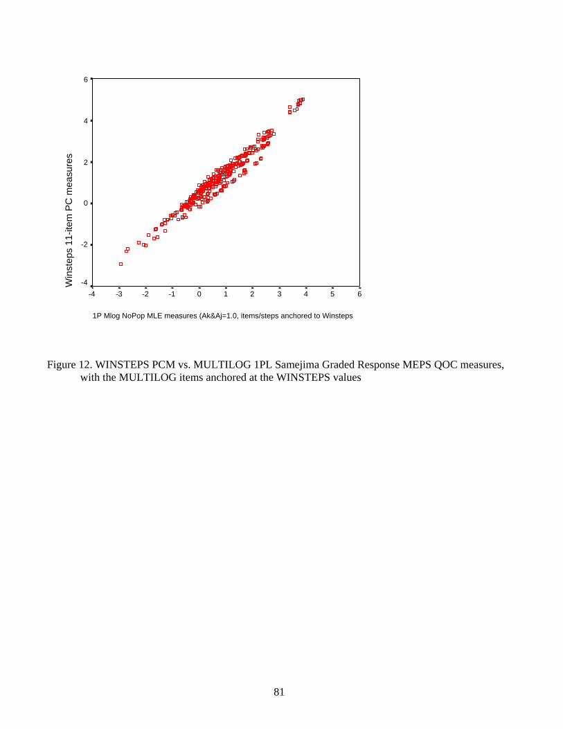
Table 13. Comparison of features of PCM, IRT, and Summated Ratings analyses 69 Figure 1. Necessary & sufficient conditions: interval scaling & measurement invariance 70 Figure 2. Variable map 71 Figure 3. Most probable response plot 72 Figure 4. QOC person measures, 2 category vs. 4-category items 73 Figure.5 Comparison of item calibrations across random samples, and by median split 74 Figure 6. Comparison of item calibrations: Public HMO vs. Private HMO vs. Medicare 75 Figure 7. Plot of non-linear ratings against linear QOC measures, for item 2 76 Figure 8. Plot of scores against linear QOC measures 77 Figure 9. Plot of person scores against linear QOC measures 78 Figure 10. Plot of item scores against linear QOC item calibrations 79 Figure 11. WINSTEPS PCM vs. MULTILOG 1PL Samejima
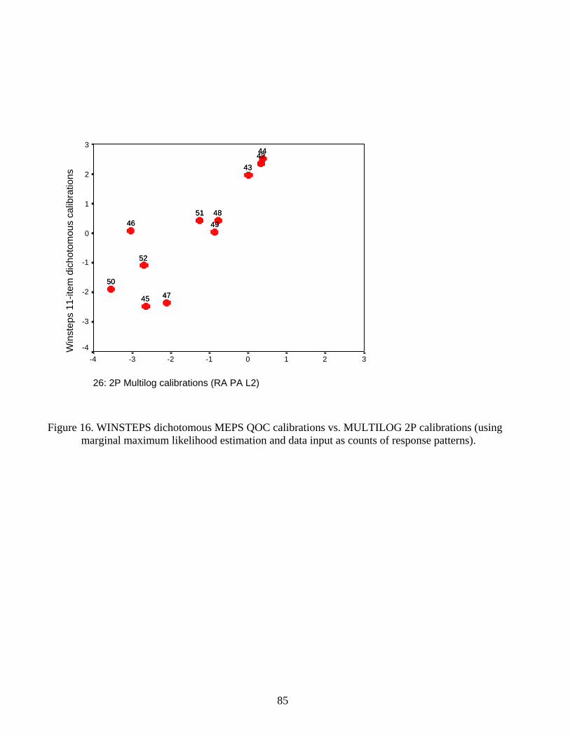
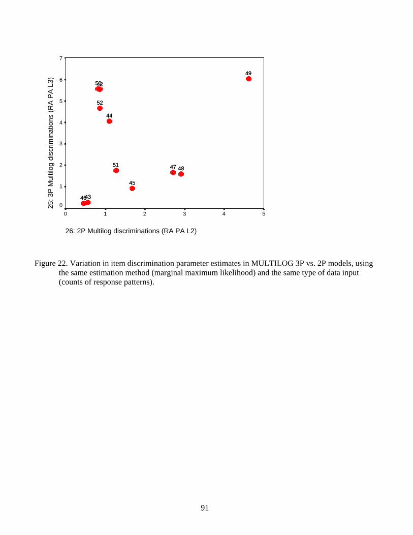
Graded Response Model measures 80 Figure 12. WINSTEPS PCM vs. MULTILOG 1PL measures (anchored) 81 Figure 13. WINSTEPS PCM vs. MULTILOG 1PL measures (discrimination=1.8) 82 Figure 14. WINSTEPS dichotomous calibrations vs. MULTILOG 1PL calibrations 83 Figure 15. WINSTEPS dichotomous measures vs. MULTILOG 1PL measures 84 Figure 16. WINSTEPS dichotomous calibrations vs. MULTILOG 2PL calibrations 85 Figure 17. WINSTEPS dichotomous calibrations vs. MULTILOG 3PL calibrations 86 Figure 18. WINSTEPS dichotomous measures vs. MULTILOG 2PL measures 87 Figure 19. WINSTEPS dichotomous measures vs. MULTILOG 3PL measures 88 Figure 20. MULTILOG 3PL vs. MULTILOG 2PL maximum a posteriori measures 89 Figure 21. Variation in item discrimination parameter estimates by type of data input 90 Figure 22. Variation in item discrimination parameter estimates by model 91
3
FUNDAMENTAL MEASUREMENT FOR HEALTH SERVICES RESEARCH
ABSTRACT
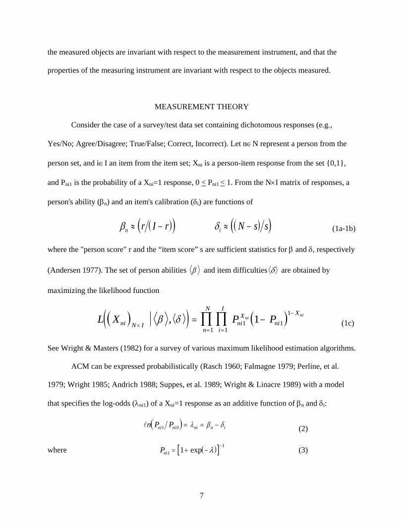
Science advances on the basis of linear measurement systems that are invariant across
different experimental conditions. However, most survey-based health sciences research employs
measures that have never been tested for invariance. This study describes and demonstrates the
mathematical properties underlying the additive formulations of probabilistic conjoint
measurement (PCM), which provide the necessary and sufficient conditions for fundamental
measurement. As a demonstration, PCM was applied to data from 23,767 persons who responded
to the Medical Expenditure Panel Survey (MEPS) conducted by the Agency for Healthcare
Research and Quality (AHRQ; formerly the Agency for Health Care Policy and Research
(AHCPR)). This demonstration includes tests of five hypotheses: (1) that the quality of care
(QOC) variable is quantitative, (2) that the data’s ordering of the survey items and rating
categories is meaningful, (3) that the respondent measurement order remains constant over item
subsamples, and that the item calibration order remains constant over respondent subsamples, (4)
that there are no differences among the measures associated with respondents belonging to one
or another of several different forms of insurance coverage (Private HMO, Public HMO, and
Medicare), and (5) that each of three approaches to measurement (PCM, Item Response Theory,
and the commonly used method of summated ratings) have specific scientific strengths and
weaknesses that make them appropriate for general use as scientific measurement methods. None
of the hypotheses were rejected, though (3) and (5) are strongly qualified. The results indicate
two general conclusions: (1) PCM offers new insights into theories of QOC, and (2) it is possible
to construct fundamental measurement systems of QOC variables. Finally, since QOC
fundamental measurement systems can be constructed, it will be possible to equate and interpret
the responses of different QOC surveys in the same metric.
4
INTRODUCTION
“It is a scientific platitude that there can be neither precise control nor prediction of
phenomena without measurement…. It is nearly useless to have an exactly formulated
quantitative theory if empirically feasible methods of measurement cannot be developed for a
substantial portion of the quantitative concepts of the theory. Given a physical concept like that
of mass or a psychological concept like that of habit strength, the point of the theory of
measurement is to lay bare the structure of a collection of empirical relations which may be used
to measure the characteristic of empirical phenomena corresponding to the concept. Why a
collection of relations? From an abstract standpoint a set of empirical data consists of a
collection of relations between specified objects …The major source of difficulty in providing an
adequate theory of measurement is to construct relations which have an exact and reasonable
numerical interpretation and yet also have a technically practical interpretation” (Scott & Suppes,
1958).
The research reported here asks what empirical relations in quality of care survey data
might provide the measurement quality needed for both exact numerical and technically practical
interpretations. If a variable is to be measured precisely, then it needs to be 1) measurable on a
linear (interval or ratio) scale, where 2) the measurement of objects does not depend on which
measurement instrument is used, and 3) the properties of the measuring instrument do not change
with the object measured. For instance, a person's height 1) represents a linear magnitude, 2)
remains the same, no matter which ruler is used, and 3) the markings on the ruler remain in the
same positions, regardless of who is measured.
That the three basic requirements of measurement can be met in the physical sciences is
strikingly obvious. That these requirements can be attained in the health sciences is not so
obvious, since most health science variables (e.g., pain, quality of life, etc.) are latent. Common
practice assigns numeric values to observations of these variables and analyzes them as though
they represent linear magnitudes. Such assignments arbitrarily depend on the perceptions of the
5
experimenter and the particular persons surveyed. Measurements based on such assignments are
never linear or generalizable across laboratories.
For example, summed rating scale responses are typically treated as linear measures.
Consider a 3-category response format Disagree (1) / Neutral (2) / Agree (3) employed for a
particular survey. Although the assigned numbers show a difference of 1 between successive
categories, their true distances are unknown and may be highly variable (Wilson 1971; Duncan
& Fisher 2000). This pattern indicates that 1) the highest quality of care or satisfaction with
services is usually associated with the physician; 2) somewhat less quality is associated with
nursing, allied health staff, and general access to care; 3) less quality yet is found with regard to
47
office staff, making appointments, and telephone access; and 4) the least quality is associated
with waiting room comfort and cleanliness, and parking availability.
Plainly, the existence of this continuum does not imply that waiting room comfort and
cleanliness ought to be improved so as to provoke ratings equivalent to those obtained by the
physician. On the contrary, in the spirit of continuous quality assessment and improvement
(McLaughlin & Kaluzny 1999), the theoretical stability of the QOC continuum across
instruments, providers, and health care consumers ought to be employed as the criterion
reference against which quality improvement efforts are evaluated. Instead of adopting the
quality control approach’s futile efforts to cut off the low quality tail of the measurement
distribution, the point is instead to move the entire distribution up the ruler to an overall higher
quality.
Should this as yet informally documented pattern prove to be stable across brands of
instruments, as has been found to be the case with clinician-assigned ratings of physical
functioning (Fisher 1997a, 1997b; Fisher, Harvey, Taylor, et al. 1995), it should be possible to
calibrate a reference standard metric to which all instruments measuring QOC would be
traceable, using methods adapted from the existing standard procedures of metrology (Mandel
1977 1978; Wernimont 1977, 1978; Pennella 1997).
CONCLUSION
Although the MEPS QOC instrument will need certain refinements to optimize its
functioning, PCM analysis provides clear evidence that fundamental measurement systems can
be created for QOC variables.
Given a sufficiently reliable QOC measurement system, it should be possible to equate
different QOC measures together so as to make them traceable to a reference standard metric.
Fisher and Karabatsos (2003) compare PCM analyses of the MEPS QOC items with similar
48
analyses of the QOC-specific items from the Consumer Assessment of Health Plans Study
(CAHPS, version 2.0 Adult Core items), also funded by AHRQ. Given that there are no items
common to both the MEPS and the CAHPS, and that the MEPS measurement reliability is so
low, equating would probably not be viable. As an alternative, a new instrument has been
designed according to the PCM principles described above and following the content included in
the MEPS and CAHPS QOC scales. Research on this scale continues.
In practice, much research presented in the context of IRT, Rasch measurement, latent
trait theory, or conjoint analysis is, or strives, in effect, to be PCM. But the hypotheses tested in
these reports vary widely, as does the quality of their execution. The present report itself is
undoubtedly far from perfect, but it is hoped that it may be taken as a contribution toward the
development of improved research standards in the human sciences.
49
References Cited Andersen, E. B. (1977). Sufficient statistics and latent trait models. Psychometrika, 42(1), 69-81. Andrich, D. (1988). Sage University Paper Series on Quantitative Applications in the Social Sciences. Vol. series no. 07-068: Rasch models for measurement. Beverly Hills, California: Sage Publications.
Andrich, D. (1989). Distinctions between assumptions and requirements in measurement in the social sciences. In J. A. Keats, R. Taft, R. A. Heath & S. H. Lovibond (Eds.), Mathematical and Theoretical Systems: Proceedings of the 24th International Congress of Psychology of the International Union of Psychological Science, Vol. 4 (pp. 7-16). North-Holland: Elsevier Science Publishers.
Angelico, D., Fisher, W. P., Jr. (2000a). Measuring patient satisfaction in the LSU Health Care Services Division. International Objective Measurement Workshops, New Orleans, April.
Angelico, D., Fisher, W. P., Jr. (2000b). Reliability in the measurement of patient satisfaction. Sixth AHRQ/CDC Building Bridges Conference. Atlanta, April. Bergling, B. M. (1999, Sep). Developmental changes in reasoning strategies: Equating scales for two age groups. European Psychologist, 4(3), 157-164.
Bernhard, J., Cella, D. F., Coates, A. S., Fallowfield, L., Ganz, P. A., Moinpour, C. M., Mosconi, P., Osoba, D., Simes, J., & Hurny, C. (1998, Mar). Missing quality of life data in cancer clinical trials: Serious problems and challenges. [Review] [42 refs]. Statistics in Medicine, 17(5-7), 15-Apr. Birnbaum, A. (1968). Some latent trait models and their use in inferring an examinee's ability. In F. M. Lord & M. R. Novick (Eds.), Statistical theories of mental test scores. Reading, Massachusetts: Addison-Wesley. Brogden, H. E. (1977). The Rasch model, the law of comparative judgment and additive conjoint measurement. Psychometrika, 42, 631-634.
Busemeyer, J. R., & Wang, Y.-M. (2000, March). Model comparisons and model selections based on generalization criterion methodology. Journal of Mathematical Psychology, pp. 171-189. Cherryholmes, C. (1988). Construct validity and the discourses of research. American Journal of Education, 96(3), 421-457. Cliff, N. (1982). What is and isn't measurement. In G. Keren (Ed.), Statistical and methodological issues in psychology and social sciences research (pp. 3-38). Hillsdale, New Jersey: Lawrence Erlbaum Associates. Cliff, N. (1989). Ordinal consistency and ordinal true scores. Psychometrika, 54, 75-91. Cliff, N. (1992). Abstract measurement theory and the revolution that never happened. Psychological Science, 3, 186-190. Cohen, J., Monheit, A. C., Beauregard, K. M., Cohen, S., Lefkowitz, D., Potter, D., Sommers, J., Taylor, A., & Arnett, R. (1996-97, Winter). The Medical Expenditure Panel Survey: A national health information resource. Inquiry, 33(4), 373-89. Connolly, A. J., Nachtman, W., & Pritchett, E. M. (1971). Keymath: Diagnostic Arithmetic Test. Circle Pines, MN: American Guidance Service. Dawson, T. L. (2000). Moral and evaluative reasoning across the life-span. Journal of Applied Measurement, 1(4), 346-371.
50
Duncan, O. D. (1984). Notes on social measurement: Historical and critical. New York: Russell Sage Foundation. Embretson, S. E. (1996, September). Item Response Theory models and spurious interaction effects in factorial ANOVA designs. Applied Psychological Measurement, 20(3), 201-212. Falmagne, J.-C. (1979). On a class of probabilistic conjoint measurement models: Some diagnostic properties. Journal of Mathematical Psychology, 19, 73-88. Fisher, R. A. (1922). On the mathematical foundations of theoretical statistics. Philosophical Transactions of the Royal Society of London, A, 222, 309-368.
Fisher, W. P., Jr. (1992a). Measuring rehabilitation client satisfaction. Midwest Objective Measurement Seminar, University of Chicago, December.
Fisher, W. P., Jr. (1992b). Objectivity in measurement: A philosophical history of Rasch's separability theorem. In M. Wilson (Ed.), Objective measurement: Theory into practice. Vol. I (pp. 29-58). Norwood, New Jersey: Ablex Publishing Corporation. Fisher, W. P., Jr. (1993, April). Measurement-related problems in functional assessment. The American Journal of Occupational Therapy, 47(4), 331-338. Fisher, W. P., Jr. (1994). The Rasch debate: Validity and revolution in educational measurement. In M. Wilson (Ed.), Objective measurement: Theory into practice. Vol. II (pp. 36-72). Norwood, New Jersey: Ablex Publishing Corporation. Fisher, W. P., Jr. (1997a). Physical disability construct convergence across instruments: Towards a universal metric. Journal of Outcome Measurement, 1(2), 87-113. Fisher, W. P., Jr. (1997b, June). What scale-free measurement means to health outcomes research. Physical Medicine & Rehabilitation State of the Art Reviews, 11(2), 357-373. Fisher, W. P., Jr. (1998). A research program for accountable and patient-centered health status measures. Journal of Outcome Measurement, 2(3), 222-239. Fisher, W. P., Jr. (2000a). Objectivity in psychosocial measurement: What, why, how. Journal of Outcome Measurement, 4(2), 527-563.
Fisher, W. P., Jr. (2000b). Survey design recommendations. Popular Measurement, 3(1), 58-9. Fisher, W. P., Jr., Harvey, R. F., & Kilgore, K. M. (1995). New developments in functional assessment: Probabilistic models for gold standards. NeuroRehabilitation, 5(1), 3-25.
Fisher, W. P., Jr., Harvey, R. F., Taylor, P., Kilgore, K. M., & Kelly, C. K. (1995). Rehabits: A common language of functional assessment. Archives of Physical Medicine and Rehabilitation, 76, 113-122.
Fisher, William P., Karabatsos, G. (2000a). Fundamental measurement with MEPS/CAHPS quality of care data. Presented at the Third International Outcome Measurement Conference. Northwestern Memorial Hospital, Chicago, June.
Fisher, W. P., Jr., Karabatsos, G. (2000b). Quality of care metrology: New possibilities for generalized quantification. American Public Health Association, Boston, November. Goldstein, H. (1979). Consequences of using the Rasch model for educational assessment. British Educational Research Journal, 5(2), 211-220. Goldstein, H., & Blinkhorn, S. (1977). Monitoring educational standards -- An inappropriate model. Bulletin of the British Psychological Society, 30, 309-311. Green, S. B., Lissitz, R. W., & Mulaik, S. A. (1977, Winter). Limitations of coefficient alpha as an index of test unidimensionality. Educational and Psychological Measurement, 37(4), 827-833.
51
Gustafsson, J.-E. (1980). Testing and obtaining fit of data to the Rasch model. British Journal of Mathematical and Statistical Psychology, 33, 205-233. Guttman, L. (1985). The illogic of statistical inference for cumulative science. Applied Stochastic Models and Data Analysis, 1, 3-10. Hahn, E., Webster, K. A., Cella, D., & Fairclough, D. (1998, Mar). Missing data in quality of life research in Eastern Cooperative Oncology Group (ECOG) clinical trials: Problems and solutions. Statistics in Medicine, 17(5-7), 15-Apr. Haley, S. M., McHorney, C. A., & Ware, J. E., Jr. (1994). Evaluation of the MOS SF-36 physical functioning scale (PF-10): I. unidimensionality and reproducibility of the Rasch item scale. Journal of Clinical Epidemiology, 47(6), 671-684. Hambleton, R. (Editor). (1983). Applications of Item Response Theory (IRT). Vancouver, BC: Educational Research Institute of British Columbia. Hambleton, R. K., & Cook, L. L. (1977). Latent trait models and their use in the analysis of educational test data. Journal of Educational Measurement, 14(2), 75-96. Hambleton, R. K., & Swaminathan, H. (1985). Item response theory: Principles and applications. Hingham, MA: Kluwer. Heilbron, J. L. (1993). Weighing imponderables and other quantitative science around 1800. Historical studies in the physical and biological sciences (Vol. 24 (Supplement), Part I, pp. 1-337). Berkeley, California: University of California Press.
Holm, K., & Kavanagh, J. (1985). An approach to modifying self-report instruments. Research in Nursing and Health, 8, 13-18. Hulin, C. L., Drasgow, F., & Parsons, C. K. (1983). Item response theory: Applications to psychological measurement. Homewood: Dow Jones Irwin.
Karabatsos, G. (1999a, April). Rasch versus 2PL/3PL in axiomatic measurement theory. In Session 53.50, K. F. Cook (Chair), Theoretical issues in Rasch measurement. American Educational Research Association. Montreal, Canada: Rasch Measurement SIG. Karabatsos, G. (1999b). Representational measurement theory as a basis for model selection in item-response theory. Society of Mathematical Psychology. Santa Cruz, CA.
Karabatsos, G., Fisher, W. P., Jr. (2000). MEPS and CAHPS quality of care calibration results. American Public Health Association, Boston, November. Kolen, M. J., & Brennan, R. L. (1995). Test equating. New York: Springer. Krantz, D. H., Luce, R. D., Suppes, P., & Tversky, A. (1971). Foundations of measurement. Volume 1: Additive and polynomial representations. New York, New York: Academic Press. Kruskal, W. H. (1960). Some remarks on wild observations. Technometrics, 2, 1-3. (Rpt. in H. H. Ku, (Ed.). (1969). Precision measurement and calibration (pp. 346-8). Washington, DC: National Bureau of Standards). Kuhn, T. S. (1961). The function of measurement in modern physical science. Isis, 52(168), 161-193. (Rpt. in The essential tension: Selected studies in scientific tradition and change (pp. 178-224). Chicago, Illinois: University of Chicago Press). Likert, R. (1932). A technique for the measurement of attitudes. Archives of Psychology, 140, 5-55. Linacre, J. M. (1993). Rasch generalizability theory. Rasch Measurement Transactions, 7(1), 283-284; Linacre, J. M. (1997). Instantaneous measurement and diagnosis. Physical Medicine and Rehabilitation State of the Art Reviews, 11(2), 315-324.
52
Linacre, J. M. (1998). Detecting multidimensionality: Which residual data-type works best? Journal of Outcome Measurement, 2(3), 266-83. Linacre, J. M. (1999). Investigating rating scale category utility. Journal of Outcome Measurement, 3(2), 103-22. Lord, F. M. (1980). Applications of item response theory to practical testing problems. Hillsdale, New Jersey: Lawrence Erlbaum. Lord, F. M. (1983). Small N justifies Rasch model. In D. J. Weiss (Ed.), New horizons in testing: Latent trait test theory and computerized adaptive testing (pp. 51-61). New York, New York: Academic Press, Inc. Lord, F. M., & Novick, M. R. (Eds.). (1968). Statistical theories of mental test scores. Reading, Massachusetts: Addison-Wesley. Luce, R. D., & Tukey, J. W. (1964). Simultaneous conjoint measurement: A new kind of fundamental measurement. Journal of Mathematical Psychology, 1(1), 1-27. Ludlow, L. H., & Haley, S. M. (1995, December). Rasch model logits: Interpretation, use, and transformation. Educational and Psychological Measurement, 55(6), 967-975. Ludlow, L. H., & Haley, S. M. (1992). Polytomous Rasch models for behavioral assessment: The Tufts Assessment of Motor Performance. In M. Wilson (Ed.), Objective measurement: Theory into practice, Volume 1 (pp. 121-137). Norwood, New Jersey: Ablex Publishing Corporation. Lumsden, J. (1978). Tests are perfectly reliable. British Journal of Mathematical and Statistical Psychology, 31, 19-26. Lunz, M. E., Bergstrom, B. A., & Gershon, R. C. (1994). Computer adaptive testing. International Journal of Educational Research, 21(6), 623-634. Maor, E. (1994). e: The story of a number. Princeton, New Jersey: Princeton University Press. Mandel, J. (1977, March). The analysis of interlaboratory test data. ASTM Standardization News, 5, 17-20, 56. Mandel, J. (1978, December). Interlaboratory testing. ASTM Standardization News, 6, 11-12. Masters, G. N. (1986). Item discrimination: When more is worse. Journal of Educational Measurement, 24, 15-29. McDowell, I., & Newell, C. (1996). Measuring health: A guide to rating scales and questionnaires. 2d edition. Oxford: Oxford University Press. McHorney, C. A. (1997, Oct 15). Generic health measurement: Past accomplishments and a measurement paradigm for the 21st century. [Review] [102 refs]. Annals of Internal Medicine, 127(8 Pt 2), 743-50. McLaughlin, C. P., & Kaluzny, A. D. (1999). Continuous quality improvement in health care: Theory, implementation, and applications. Gaithersburg, Maryland: Aspen Publishers, Inc.
Meehl, P. E. (1967). Theory-testing in psychology and physics: A methodological paradox. Philosophy of Science, 34(2), 103-115. Merbitz, C., Morris, J., & Grip, J. (1989). Ordinal scales and the foundations of misinference. Archives of Physical Medicine and Rehabilitation, 70, 308-312. Messick, S. (1975, October). The standard problem: Meaning and values in measurement and evaluation. American Psychologist, 30, 955-966. Michell, J. (1986). Measurement scales and statistics: A clash of paradigms. Psychological Bulletin, 100, 398-407.
53
Michell, J. (1990). An introduction to the logic of psychological measurement. Hillsdale, New Jersey: Lawrence Erlbaum Associates. Michell, J. (1997). Quantitative science and the definition of measurement in psychology. British Journal of Psychology, 88, 355-383. Michell, J. (1999). Measurement in psychology: A critical history of a methodological concept. Cambridge: Cambridge University Press. Michell, J. (2000, October). Normal science, pathological science and psychometrics. Theory & Psychology, 10(5), 639-667. Mundy, B. (1986). On the general theory of meaningful representation. Synthese, 67, 391-437. Ottenbacher, K. J., & Tomchek, S. D. (1993). Measurement in rehabilitation research: Consistency versus consensus. Physical Medicine and Rehabilitation Clinics of North America, 4(3), 463-473. Pennella, C. R. (1997). Managing the metrology system. Milwaukee, WI: ASQ Quality Press. Perline, R., Wright, B. D., & Wainer, H. (1979). The Rasch model as additive conjoint measurement. Applied Psychological Measurement, 3(2), 237-255. Phillips, S. E. (1986). The effects of the deletion of misfitting persons on vertical equating via the Rasch model. Journal of Educational Measurement, 23(2), 107-118. Rasch, G. (1960). Probabilistic models for some intelligence and attainment tests (reprint, with Foreword and Afterword by B. D. Wright, Chicago: University of Chicago Press, 1980). Copenhagen, Denmark: Danmarks Paedogogiske Institut. Revicki, D. A., & Cella, D. F. (1997, Aug). Health status assessment for the twenty-first century: Item response theory item banking and computer adaptive testing. Quality of Life Research, 6(6), 595-600. Roche, J. (1998). The mathematics of measurement: A critical history. London: The Athlone Press. Roskam, E. E., & Jansen, P. G. W. (1984). A new derivation of the Rasch model. In E. DeGreef & J. van Buggenhaut (Eds.), Trends in mathematical psychology. Amsterdam: Elsevier. Scott, D., & Suppes, P. (1958, June). Foundational aspects of theories of measurement. The Journal of Symbolic Logic, 23(2), 113-128. Smith, R. M. (1986). Person fit in the Rasch model. Educational and Psychological Measurement, 46, 359-372. Smith, R. M. (1988). The distributional properties of Rasch standardized residuals. Educational & Psychological Measurement, 48(3), 657-667. Smith, R. M. (1991). The distributional properties of Rasch item fit statistics. Educational and Psychological Measurement, 51, 541-565.
Smith, R. M. (1992). Applications of Rasch measurement. Chicago, Illinois: MESA Press. Smith, R. M., Schumacker, R. E., & Bush, M. J. (1998). Using item mean squares to evaluate fit to the Rasch model. Journal of Outcome Measurement, 2(1), 66-78. Sparrow, S., Balla, D., & Cicchetti, D. (1984). Interview edition, survey form manual, Vineland Behavior Scales. Circle Pines, MN: American Guidance Services, Inc. Streiner, D. L., & Norman, G. R. (1995). Health measurement scales: A practical guide to their development and use, 2d edition. New York, New York: Oxford University Press.
54
Stucki, G., Daltroy, L., Katz, N., Johannesson, M., & Liang, M. H. (1996). Interpretation of change scores in ordinal clinical scales and health status measures: The whole may not equal the sum of the parts. Journal of Clinical Epidemiology, 49(7), 711-717. Suppes, P., Krantz, D., Luce, R. D., & Tversky, A. (1989). Foundations of measurement, Volume II: Geometric and probabilistic representations. New York: Academic Press.
Thissen, D. (1991). MULTILOG, V. 6. Chicago, Illinois: Scientific Software, Inc. Thurstone, L. L. (1926). The scoring of individual performance. Journal of Educational Psychology, 17, 446-457.
Thurstone, L. L. (1928). Attitudes can be measured. American Journal of Sociology, XXXIII, 529-544. Reprinted in L. L. Thurstone, The Measurement of Values. Midway Reprint Series. Chicago, Illinois: University of Chicago Press, 1959, pp. 215-233. Troxel, A. B., Fairclough, D. L., Curran, D., & Hahn, E. (1998). Statistical analysis of quality of life with missing data in cancer clinical trials: Problems and solutions. Statistics in Medicine, 17, 547-59. van der Linden, W. J., & Hambleton, R. K. (1997). Item response theory: A brief history. Handbook of Modern Item Response Theory (IRT)W. J. van der Linden & R. K. Hambleton (Eds.), (pp. 1-28). New York: Springer-Verlag. Wernimont, G. (1977, March). Ruggedness evaluation of test procedures. ASTM Standardization News, 5, 13-16. Wernimont, G. (1978, December). Careful intralaboratory study must come first. ASTM Standardization News, 6, 11-12. Whiteneck, G. G., Charlifue, S. W., Gerhart, K. A., Overholser, J. D., & Richardson, G. N. (1992, June). Quantifying handicap: A new measure of long-term rehabilitation outcomes. Archives of Physical Medicine and Rehabilitation, 73(6), 519-526. Wilson, T. P. (1971). Critique of ordinal variables. Social Forces, 49, 432-444. Wimsatt, W. C. (1981). Robustness, reliability and overdetermination. In M. B. Brewer & B. E. Collins (Eds.), Scientific inquiry and the social sciences. San Francisco: Jossey-Bass. Wolfe, E. W. (2000). Equating and item banking with the Rasch model. Journal of Applied Measurement, 1(4), 409-434. Wood, R. (1978). Fitting the Rasch model: A heady tale. British Journal of Mathematical and Statistical Psychology, 31, 27-32. Woodcock, R. W. (1973). Woodcock Reading Mastery Tests. Circle Pines, MN: American Guidance Service, Inc. Woodcock, R. W. (1999). What can Rasch-based scores convey about a person's test performance? In S. E. Embretson & S. L. Hershberger (Eds.), The new rules of measurement: What every psychologist and educator should know. Hillsdale, NJ: Lawrence Erlbaum Associates.
Wright, B. D. (1977a). Misunderstanding the Rasch model. Journal of Educational Measurement, 14(3), 219-225. Wright, B. D. (1977b). Solving measurement problems with the Rasch model. Journal of Educational Measurement, 14(2), 97-116. Wright, B. D. (1984). Despair and hope for educational measurement. Contemporary Education Review, 3(1), 281-288. Wright, B. D. (1985). Additivity in psychological measurement. In E. Roskam (Ed.), Measurement and personality assessment. North Holland: Elsevier Science Ltd.
55
Wright, B. D. (1999). Fundamental measurement for psychology. In S. E. Embretson & S. L. Hershberger (Eds.), The new rules of measurement: What every educator and psychologist should know. Hillsdale, NJ: Lawrence Erlbaum Associates. Wright, B. D., & Linacre, J. M. (1989). Observations are always ordinal; measurements, however, must be interval. Archives of Physical Medicine and Rehabilitation, 70(12), 857-867. Wright, B. D., & Linacre, J. M. (1999). A User's Guide to WINSTEPS Rasch-Model Computer Program, v. 2.94. Chicago: MESA Press. Wright, B. D., & Masters, G. N. (1982). Rating scale analysis: Rasch measurement. Chicago: MESA Press. Wright, B. D., & Stone, M. H. (1979). Best test design: Rasch measurement. Chicago: MESA Press. Zhu, W. (1996). Should total scores from a rating scale be used directly? Research Quarterly for Exercise and Sport, 67(3), 363-372.
56
ITEMS Person v w y z Score (1a) βn P a 1 1 1 0 3 1.1 E b 1 1 1 0 3 1.1 R c 1 0 1 0 2 0 S d 1 1 0 0 2 0 O e 1 0 0 0 1 -1.1 N f 0 0 0 1 1 -1.1 S Item Score (1b) 5 3 3 1 δi -1.6 0 0 1.6
Table 1. Six persons’ responses to a 4-item survey.
57
ITEMS v w y z βn P a .94 .75 .75 .38 1.1 E b .94 .75 .75 .38 1.1 R c .83 .50 .50 .17 0 S d .83 .50 .50 .17 0 O e .63 .25 .25 .06 -1.1 N f .63 .25 .25 .06 -1.1 δi -1.6 0 0 1.6
Table 2. The data in Table 1 expressed as probabilities.
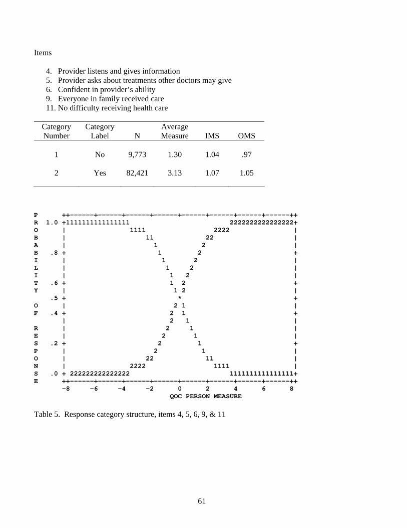
4. Provider listens and gives information 5. Provider asks about treatments other doctors may give 6. Confident in provider’s ability 9. Everyone in family received care 11. No difficulty receiving health care
Category Number
Category Label
N
Average Measure
IMS
OMS
1
No
9,773
1.30
1.04
.97
2
Yes
82,421
3.13
1.07
1.05
P ++------+------+------+------+------+------+------+------++ R 1.0 +1111111111111111 2222222222222222+ O | 1111 2222 | B | 11 22 | A | 1 2 | B .8 + 1 2 + I | 1 2 | L | 1 2 | I | 1 2 | T .6 + 1 2 + Y | 1 2 | .5 + * + O | 2 1 | F .4 + 2 1 + | 2 1 | R | 2 1 | E | 2 1 | S .2 + 2 1 + P | 2 1 | O | 22 11 | N | 2222 1111 | S .0 + 222222222222222 1111111111111111+ E ++------+------+------+------+------+------+------+------++ -8 -6 -4 -2 0 2 4 6 8
Items 1. How difficult is it to get appointments? 3. How difficult is it to contact provider by phone?
Category Number
Category Label
N
Average Measure
IMS
OMS
Step Threshold
1
Very
Difficult
2,989
−0.59
.95
.91
2
Somewhat Difficult
4,892
0.07
.94
.84
3
Not Too Difficult
11,630
0.82
.93
.80
4
Not at all Difficult
13,390
1.90
1.16
1.11
−0.72 (1→2) −0.43 (2→3) 1.16 (3→4)
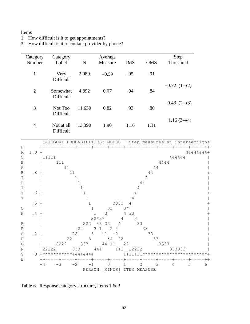
CATEGORY PROBABILITIES: MODES - Step measures at intersections P ++-----+-----+-----+-----+-----+-----+-----+-----+-----+-----++ R 1.0 + 44444444+ O |11111 444444 | B | 111 4444 | A | 11 44 | B .8 + 11 44 + I | 1 4 | L | 1 44 | I | 1 4 | T .6 + 1 4 + Y | 1 4 | .5 + 1 3333 4 + O | 1 33 3* | F .4 + 1 3 4 33 + | 22*2* 4 3 | R | 222 *3 22 4 33 | E | 22 3 1 2 4 33 | S .2 + 22 3 11 *2 33 + P | 22 3 *4 22 33 | O | 2222 333 44 11 22 3333 | N |22222 333 444 111 22222 333333 | S .0 +***********44444444 1111111************************+ E ++-----+-----+-----+-----+-----+-----+-----+-----+-----+-----++ -4 -3 -2 -1 0 1 2 3 4 5 6 PERSON [MINUS] ITEM MEASURE Table 6. Response category structure, items 1 & 3
62
Item 2. How long is the usual wait for a medical appointment?
Category Number
Category Label
N
Average Measure
IMS
OMS
Step Threshold
1
>2 hours
250
0.38
1.37
1.44
2
1-2 hours
1,111
0.89
1.24
1.29
3
31 to 59 minutes
1,831
1.34
1.17
1.20
4
16 to 30 minutes
5,212
1.95
1.21
1.20
2.69 (1→2) 1.11 (2→3) 1.06 (3→4) 0.43 (4→5)
5
5-15
minutes
7,387
2.92
1.24
1.16
4.43 (5→6)
6 <5 minutes
669 3.33 1.82 1.26
CATEGORY PROBABILITIES: MODES - Step measures at intersections P ++-----+-----+-----+-----+-----+-----+-----+-----+-----+-----++ R 1.0 + + O | | B | | A | 6| B .8 +1 5555 6 + I | 1 555 555 66 | L | 1 5 55 66 | I | 11 55 55 6 | T .6 + 1 5 5 6 + Y | 1 5 5 6 | .5 + 1 222 5 5* + O | *2 22 444444* 66 5 | F .4 + 22 1 2 4 5 4 6 5 + | 22 1 2 4 5 44 6 5 | R | 2 1 3**3 5 4 6 55 | E | 22 1 33 42 33 5 44 66 5 | S .2 +2 3* 4 2 *3 44 66 55 + P | 33 *4 ** 33 44 66 5| O | 333 44 11 5 22 33 6**4 | N | 3333 444 55**1 222 333366666 444444 | S .0 +***************66666*****************************************+ E ++-----+-----+-----+-----+-----+-----+-----+-----+-----+-----++ -4 -3 -2 -1 0 1 2 3 4 5 6 PERSON [MINUS] ITEM MEASURE Table 7. Response category structure, item 2
63
ITEMS LOWDIF MIDDIFF HIDIFF43,44,47,49,
51,5242,45,46,48,
50LOWDIFF Pearson
Correlation1.000 .718 .255 .706 .524
Sig. (2-tailed)
. .000 .000 .000 .000
N 16121 16069 11476 16121 16121MIDDIFF Pearson
Correlation.718 1.000 .470 .875 .680
Sig. (2-tailed)
.000 . .000 .000 .000
N 16069 16083 11476 16069 16069HIDIFF Pearson
Correlation.255 .470 1.000 .889 .799
Sig. (2-tailed)
.000 .000 . .000 .000
N 11476 11476 11476 11476 11476RandomSelection
43,44,47,49,51,52
Pearson Correlation
.706 .875 .889 1.000 .813
Sig. (2-tailed)
.000 .000 .000 . .000
N 16121 16069 11476 16121 16121RandomSelection
42,45,46,48,50
Pearson Correlation
.524 .680 .799 .813 1.000
Sig. (2-tailed)
.000 .000 .000 .000 .
N 16121 16069 11476 16121 16121** Correlation is significant at the 0.01 level (2-tailed). Table 8. Comparison of QOC person measures across several item-subset conditions (step-anchored
analysis).
64
N=6,094 ANALYZABLE FOR LOW MEDIAN GROUP N=4,915 ANALYZABLE FOR HIGH MEDIAN GROUP Correlations
** Correlation is significant at the 0.01 level (2-tailed). * Correlation is significant at the 0.05 level (2-tailed). Table 9. Correlation analysis --Comparison of item calibrations across random samples, and by median
split (unanchored analysis).
65
Correlations MEDIC PRVHMO PUB
MEDIC Pearson Correlation
1.000 .946 .948
Sig. (2-tailed) . .000 .000N 11 11 11
PRVHMO Pearson Correlation
.946 1.000 .958
Sig. (2-tailed) .000 . .000N 11 11 11
PUB Pearson Correlation
.948 .958 1.000
Sig. (2-tailed) .000 .000 .N 11 11 11
** Correlation is significant at the 0.01 level (2-tailed). Table 10. Correlation matrix of the item calibrations: Public HMO vs. Private HMO vs. Medicare.
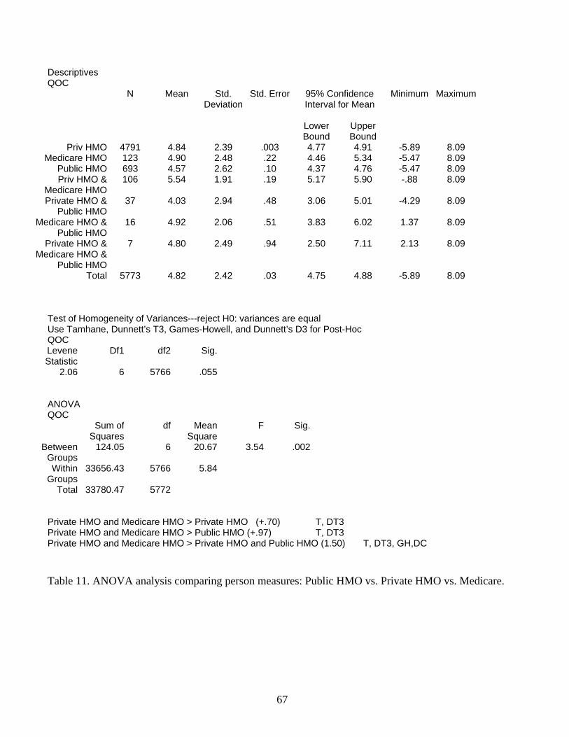
Total 5773 4.82 2.42 .03 4.75 4.88 -5.89 8.09 Test of Homogeneity of Variances---reject H0: variances are equal Use Tamhane, Dunnett’s T3, Games-Howell, and Dunnett’s D3 for Post-Hoc QOC Levene Statistic
Df1 df2 Sig.
2.06 6 5766 .055 ANOVA QOC
Sum of Squares
df Mean Square
F Sig.
Between Groups
124.05 6 20.67 3.54 .002
Within Groups
33656.43 5766 5.84
Total 33780.47 5772 Private HMO and Medicare HMO > Private HMO (+.70) T, DT3 Private HMO and Medicare HMO > Public HMO (+.97) T, DT3 Private HMO and Medicare HMO > Private HMO and Public HMO (1.50) T, DT3, GH,DC Table 11. ANOVA analysis comparing person measures: Public HMO vs. Private HMO vs. Medicare.
67
MOST MISFITTING RESPONSE STRINGS ITEM OUTMNSQ |PERSON |2222221111 22222111111111111111111 |22222140009777766554403311999888877211110000522222 |66666689921111122416684433700662275644442222353333 |77777454479777600716642288877335465155447777064444 |87654125409210954444367687221521630454984321069875 high-------------------------------------------------- 5 ASKS ABOUT OTH 1.55 A|........................11........................ 2 APPT. WAITING 1.23 B|........................666.......6.6666.......... 11 [NO PROBLEMS] 1.11 C|111111.11..1111...111.....1....................... 9 [EVERYONE HAS 1.03 E|.........11....111......111....1111111111111...... 10 SATIS FAMILY .89 F|..................................3............... 4 LISTENS & GIVES .75 d|......1..............111...1111..............11111 6 CONFIDENT IN PR .44 c|............................................1..... |----------------------------------------------low- Table 12. Using fit statistics to identify inconsistent responses that do not contribute to the measurement
effort.
68
Features WINSTEPS
PCM MULTILOG
IRT SUMMED RATINGS
Starts from ordinal observations (counts of correct answers or sums of ratings)
Yes
Yes
Yes
Additive unit of measurement Yes Yes (1P only) No Estimates error Yes Yes No
Accommodates missing data Yes Yes No Implements tests of independence & double cancellation (tests
data consistency) Yes No No
Persons and items scaled on common metric Yes Yes No All statistics reported for both persons and items in same
analysis Yes No No
Provides multiples tests of construct validity Yes No No Provides multiple supports for creation of keyforms Yes No No
Parameter Separation Reliability Coefficient Yes No No Approximation of Cronbach’s alpha Yes Yes1 Yes
Error and reliability reported in both modeled and fit-adjusted forms
Yes No No
Infit Mean Square Yes No No Stdized Infit Yes No No
Outfit Mean Square Yes No No Stdized Outfit Yes No No
Pt. Biserial Correlations Yes No No Bias displacement estimates Yes No No
Plots variable maps Yes No No Data displayed in Guttman scalogram format Yes No No
Individual expected vs observed responses and residuals detailed in plots and tables
Yes No No
Infit-Outfit plots Yes No No Infit/Outfit-Measure plots Yes No No Raw score-Measure plots Yes No No
Principal Components factor analysis of residuals Yes No No Dichotomous models Yes Yes No Rating Scale models Yes Yes No Partial Credit models Yes Yes No Multifaceted models No No No
2P models No Yes No 3P models No Yes No
Samejima’s Graded model No Yes No Bock’s Nominal model No Yes No
Thissen/Steinberg multiple choice model No Yes No Tests assumption of normal population distribution No Yes No
Combines different models in single analysis Yes Yes No Table 13. Comparison of various features of typical PCM, IRT, and Summated Ratings analyses. (Many features of PCM and IRT can be applied to raw scores by competent users of generic statistical packages, such as SAS, SPSS, SYSTAT, etc.) 1 Marginal reliability (Thissen 1991, p. 4-11).
69
w x y z
p
.94
.75
.75
.38
q
.83
.50
.50
.17
r
.63
.25
.25
.06
INDEPENDENCE
w x z
p
.94
.75
.38
q
.83
.50
.17
r
.63
.25
.06
DOUBLE CANCELLATION
Figure 1. Necessary and sufficient conditions for interval scaling and measurement invariance.
70
MEASURE PERSONS MAP OF QOC ITEMS IN LOGITS
High QOC MARY .############ 6 5 .###### . . . . 4 .######## . . 3 .#
.######## . .#######
. 2 .#######
. .###### 2. Usual wait time for a medical appointment1 (1.59) .#### 3. Phone access (1.29) .### 1. Difficulty in obtaining appointments (1.22) 1 .#### .## 5. Provider asks about treatments other doctors may give2 (0.66) .# .# . 0 .## 10. Satisfied that family members can get needed care (−0.10) TOM . 7. Satisfaction with staff (−0.13) . 11. No difficulty receiving health care (−0.28) . 8. Satisfaction with QOC (−0.43) .# -1 . 9. Everyone in family received care (−0.94) . . 6. Confident in provider ability (−1.38) CINDY . 4. Provider listens and gives information (−1.49) . -2 . . .