1 Fundamentals of Atmospheric Chemistry and Astrochemistry Lectures 1‐3: an Introduction to Astrochemistry Claire Vallance e‐mail: [email protected]Some suggested reading: This is by no means an exhaustive list, just a few suggestions to get you started. Many of the articles below go beyond the material covered directly in this course. There are many other review articles and research articles available on every different aspect of astrochemistry if you want to find out more about particular areas. Relevant literature is also cited throughout these lecture notes. 1. Astrochemistry, by Andrew Shaw (textbook) 2. Ion chemistry and the interstellar medium, Theodore P. Snow and Veronica M. Bierbaum, Ann. Rev. Anal. Chem., 1 229‐259 (2008). 3. Laboratory Astrochemistry: Gas‐phase processes, Ian W. M. Smith, Ann. Rev. Astron. Astrosphys., 49, 29‐6 (2011). 4. Frontiers of Astrochemistry, David A. Williams, Faraday Discuss., 109,1‐13, (1998). 5. Laboratory astrochemistry: studying molecules under inter‐ and circumstellar conditions, D. Gerlich and M. Smith, Physica Scripta, 73, C25‐C31 (2006). 6. Formation of complex chemical species in astrochemistry (a review), V. I. Shematovich, Solar System Research, 46(6), 391‐407 (2012). 7. Aromatic hydrocarbons, diamonds, and fullerenes in interstellar space: puzzles to be solved by laboratory and theoretical astrochemistry, K. Sellgren, Spectrochimica Acta Part A, 57, 627‐642 (2001). 8. Quantum astrochemistry: prospects and examples, G. Berthier, F. Pauzat and Tao Yuanqi, J. Mol. Struct., 107, 39‐48 (1984). 9. Molecules, ices, and astronomy, D. A. Williams, W. A. Brown, S. D. Price, J. M. C.Rawlings, and S. Viti, Astronomy and Geophysics, 48, 1.25‐1.34 (2007)
Transcript
1
Fundamentals of Atmospheric Chemistry and Astrochemistry
This is by no means an exhaustive list, just a few suggestions to get you started. Many of the articles below
go beyond the material covered directly in this course. There are many other review articles and research
articles available on every different aspect of astrochemistry if you want to find out more about particular
areas. Relevant literature is also cited throughout these lecture notes.
1. Astrochemistry, by Andrew Shaw (textbook)
2. Ion chemistry and the interstellar medium, Theodore P. Snow and Veronica M. Bierbaum, Ann. Rev.
Anal. Chem., 1 229‐259 (2008).
3. Laboratory Astrochemistry: Gas‐phase processes, Ian W. M. Smith, Ann. Rev. Astron. Astrosphys.,
49, 29‐6 (2011).
4. Frontiers of Astrochemistry, David A. Williams, Faraday Discuss., 109, 1‐13, (1998).
5. Laboratory astrochemistry: studying molecules under inter‐ and circumstellar conditions, D. Gerlich
and M. Smith, Physica Scripta, 73, C25‐C31 (2006).
6. Formation of complex chemical species in astrochemistry (a review), V. I. Shematovich, Solar System
Research, 46(6), 391‐407 (2012).
7. Aromatic hydrocarbons, diamonds, and fullerenes in interstellar space: puzzles to be solved by
laboratory and theoretical astrochemistry, K. Sellgren, Spectrochimica Acta Part A, 57, 627‐642
(2001).
8. Quantum astrochemistry: prospects and examples, G. Berthier, F. Pauzat and Tao Yuanqi, J. Mol.
Struct., 107, 39‐48 (1984).
9. Molecules, ices, and astronomy, D. A. Williams, W. A. Brown, S. D. Price, J. M. C.Rawlings, and S.
Viti, Astronomy and Geophysics, 48, 1.25‐1.34 (2007)
2
Contents
1. Introduction
2. Studying the universe via spectroscopy
3. Doppler shift
4. Doppler lineshape
5. The Hubble constant and the age of the universe
6. The very early universe: the building blocks of matter
7. Hydrogen and helium nuclei
8. The first atoms
9. Star formation and nucleosynthesis of heavier elements
10. Dispersion of chemical elements
11. Cosmic abundance of the elements
12. The interstellar medium
13. Chemistry in interstellar space
14. Molecular synthesis in interstellar gas clouds
15. Ionization processes in the interstellar medium
16. Gas‐phase chemical reactions in the interstellar medium
16.1 Bond formation reactions
16.1.1 Radiative association
16.1.2 Associative detachment
16.2 Bond breaking reactions
16.2.1 Photodissociation and collisional dissociation
16.2.2 Dissociative recombination
16.3 Rearrangement reactions
16.3.1 Charge transfer
16.3.2 Neutral reaction
16.3.3 Ion‐molecule reactions
17. Neutralisation processes in the interstellar medium
18. Laboratory‐based astrochemistry
19. The grand challenge: chemical modelling of giant molecular clouds
20. The search for biological molecules
21. The diffuse interstellar bands (DIBs)
22. Overview of astrochemistry
3
An Introduction to Astrochemistry
1. Introduction
“Far out in the uncharted backwaters of the unfashionable end of the Western Spiral arm of the Galaxy lies a small unregarded yellow sun. Orbiting this at a distance of roughly ninety‐eight million miles is an utterly insignificant little blue‐green planet whose ape‐descended life forms are so amazingly primitive that they still think digital watches are a pretty neat idea.”
Douglas Adams, Hitchhiker’s Guide to the Galaxy
So far in your degree studies, you have become very well acquainted with the chemistry occurring on the
surface of the ‘utterly insignificant little blue‐green planet’ referred to above. In this course, we shall
extend our consideration of chemistry a little further to consider the rest of the universe. Much of what
we know about the universe has been learnt through applying fundamental principles from physical
chemistry to data acquired by earth‐based and space telescopes, and we will highlight some of these
principles as we proceed through the course. We will investigate the very early stages of the universe, and
the events leading to synthesis of the chemical elements, and will take a tour of the interstellar medium
(ISM), home to a rich chemistry of alien molecules that could not possibly survive on earth, yet can be
understood using the same principles that allow us to understand terrestrial chemistry.
2. Studying the universe via spectroscopy
Unlike most other areas of chemistry and physics, we cannot carry out any active experiments to study the
chemistry of the universe. Instead, all of the information we have comes from passive observations. The
data from telescopes arrives in the form of spectroscopic signatures recorded in various portions of the
electromagnetic spectrum (UV‐vis, infrared, microwave etc) for different regions of space (stars, interstellar
regions, and so on), and can be interpreted in order to establish the atomic and molecular composition of
these regions. Ground‐based telescopes are limited to studying regions of the electromagnetic spectrum in
which the earth’s atmosphere does not absorb. These include the visible‐UV window spanning 300‐900
nm, corresponding to electronic transitions; two infrared windows from 1‐5 m and 8‐20 m which can be
used to probe vibrational transitions; a window in the microwave and millimetre wave region from 1.3‐0.35
mm, which can be used to probe rotational transitions; and a radio wave window from 2‐10 m which
contains information on transitions between atomic hyperfine levels, such as the 21 cm line in atomic
hydrogen. Space telescopes are not subject to such restrictions, and can observe in any region of the
spectrum. In general, the microwave region is the most information rich, and therefore the most useful for
studying small molecules in space, followed by the infrared and UV‐vis regions.
Atoms and molecules may be identified through their absorption or emission frequencies and quantified by
their absorption or emission intensities. There are one or two additional features of analysing spectral data
from telescopes which differs from those encountered in more everyday spectroscopy. Firstly, most
transitions will be Doppler shifted, and secondly, the lineshape can provide a great deal of information on
the motion of the body under study.
4 3. Doppler shift
For velocities significantly less than the speed of light1, the observed wavelength of light absorbed or
emitted by a moving object is Doppler shifted by an amount
=
vsourcec (3.1)
Where is the transition wavelength, is the Doppler shift, vsource is the velocity of the source relative to the observer, and c is the speed of light. The Doppler shift must be taken into account when identifying
spectroscopic lines from telescope data; since the universe is expanding, such that all other astronomical
objects are moving away from the earth, often the lines will appear at wavelengths that are significantly
red‐shifted from that expected for a stationary sample. If the velocity of the source is known then the
wavelengths can be corrected for comparison with lab based or calculated spectroscopic data. If the
velocity of the source is not known then lines must be identified through a process of ‘pattern matching’,
and when a match is found they may be used to determine the velocity of the source.
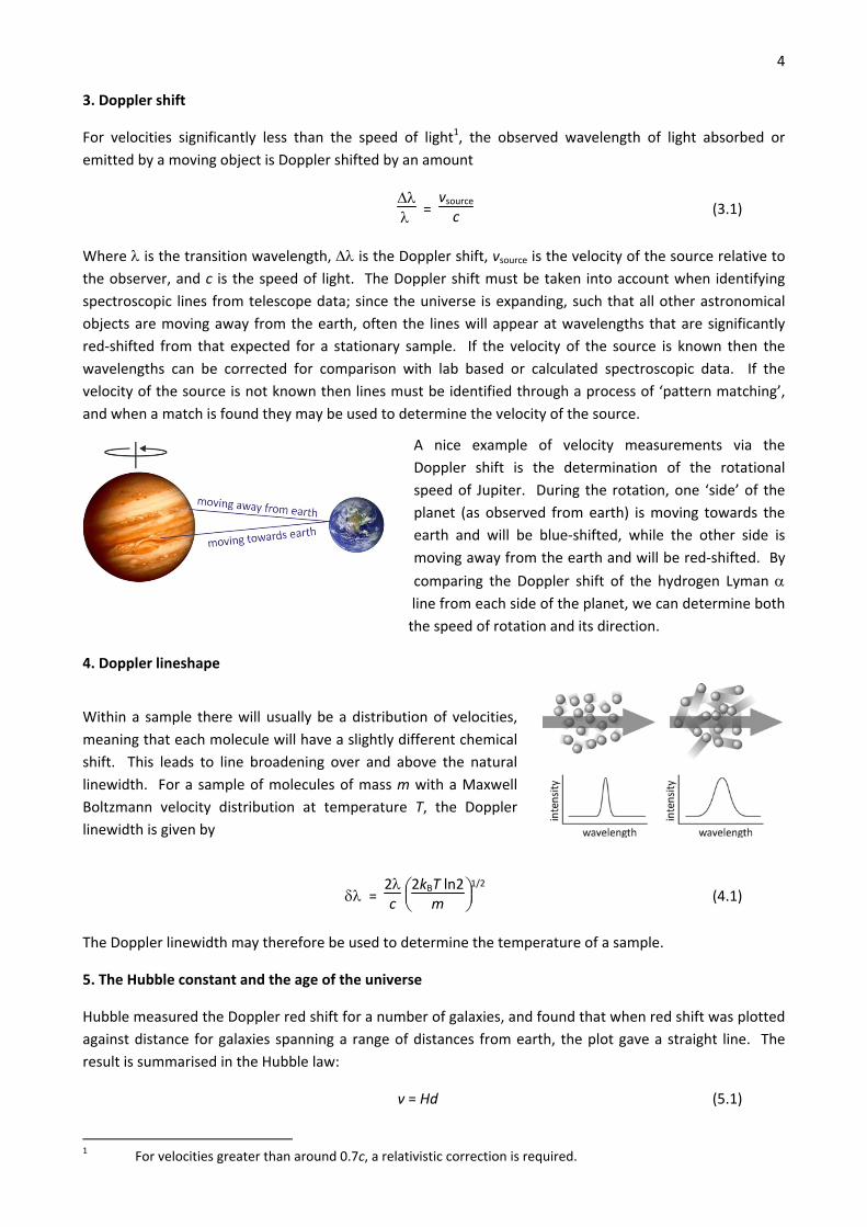
A nice example of velocity measurements via the
Doppler shift is the determination of the rotational
speed of Jupiter. During the rotation, one ‘side’ of the
planet (as observed from earth) is moving towards the
earth and will be blue‐shifted, while the other side is
moving away from the earth and will be red‐shifted. By
comparing the Doppler shift of the hydrogen Lyman line from each side of the planet, we can determine both
the speed of rotation and its direction.
4. Doppler lineshape
Within a sample there will usually be a distribution of velocities,
meaning that each molecule will have a slightly different chemical
shift. This leads to line broadening over and above the natural
linewidth. For a sample of molecules of mass m with a Maxwell
Boltzmann velocity distribution at temperature T, the Doppler
linewidth is given by
= 2c
2kBT ln2
m
1/2
(4.1)
The Doppler linewidth may therefore be used to determine the temperature of a sample.
5. The Hubble constant and the age of the universe
Hubble measured the Doppler red shift for a number of galaxies, and found that when red shift was plotted
against distance for galaxies spanning a range of distances from earth, the plot gave a straight line. The
result is summarised in the Hubble law:
v = Hd (5.1)
1 For velocities greater than around 0.7c, a relativistic correction is required.
5 Here, v is the radial velocity, H is the Hubble constant, and d is the distance. The equation summarises the
rate of recession of other galaxies, and therefore the rate at which the universe is expanding. The most
recent determination of the Hubble constant yields a value of 23 km s1 Mly1, with an error of around 10%.
Other estimates give a value between 19 and 21 km s1 Mly1. If we assume that the rate of expansion of
the universe has remained constant (this could potentially be quite a large assumption), then the age of the
universe is simply the inverse of the Hubble constant, giving an age of 13.8 billion years.
So how did chemistry originate, 13.8 billion years ago?
6. The very early universe: the building blocks of matter
Chemistry, like everything in the universe, began with the big bang. Immediately after the big bang, in
what is known as the inflationary epoch, the universe underwent extremely rapid exponential expansion,
increasing its volume by a factor of at least 1078 and expanding from subatomic dimensions to around the
size of a grapefruit. The inflationary epoch lasted until around 1032 seconds after the big bang, and this is
the earliest meaningful ‘time after the big bang’. The temperatures and pressures during this time were
both unimaginably high, and from this point on the universe continued to expand2 (non‐exponentially) and
cool rapidly.
Immediately after the inflationary epoch, the universe had cooled sufficiently for the first particles to form.
These particles formed out of pure energy. Einstein first demonstrated the equivalence and
interchangeability of matter and energy in his famous equation, E = mc2. To put this equation into context,
creation of 1 gram of mass requires an energy of 89 TeraJoules (8.9 x 10¹³ J), an almost incomprehensible
amount of energy. However, fundamental particles weigh only a tiny fraction of a gram, and their
equivalent energies, called their rest energies, are measured in MeV (mega electron volts, with 1 MeV =
1.602 x 10¹³ J). The rest energies of electrons, protons, and neutrons, three particles you will be very
familiar with, are 0.511 MeV, 938 MeV, and 950 MeV, respectively. At 1032 s after the big bang,
elementary particles began to form. These included quarks, gluons, electrons, and neutrinos. However,
with the temperature still a toasty 1027 K, it was impossible for composite particles such as protons and
neutrons to form. At this stage, the universe consisted of a unique phase of matter known as a quark‐gluon
plasma3.
2 When thinking about the big bang, most people picture matter expanding from a point in all directions in an infinite
space. While this is a convenient mental picture, it is not really correct, as it is space itself that is expanding, not matter
within space. A two dimensional analogy is to imagine living on the (two‐dimensional) surface of an inflating balloon.
The only directions you know are left, right, forwards, and backwards (up and down are meaningless on a two‐
dimensional surface). Over time, you observe that objects at rest with respect to the surface of the balloon are in fact
moving apart from each other. This is despite the fact that you have explored your entire two‐dimensional world and not
found any edge or ‘outside’ for it to expand into. Similarly, we note that other galaxies appear to be receding from our
galaxy. However, the galaxies are not really travelling through space away from us, like fragments from a ‘big bang
bomb’; instead, the space between the galaxies and us is expanding, and this expansion is happening simultaneously at
every position in the universe. This analogy was taken from the excellent article ‘Misconceptions about the big bang’ from
the March 2005 edition of Scientific American, available online for interested readers at
http://space.mit.edu/~kcooksey/teaching/AY5/MisconceptionsabouttheBigBang_ScientificAmerican.pdf. Note that since
the total energy in the universe is a constant, as the volume of the universe increases, the energy density, and therefore
the temperature, must decrease as the universe expands.
3 Physicists are putting a great deal of effort into recreating this particularly fascinating state of matter, in which the strong
interaction is overcome and free quarks and gluons are observed. As far as we know, this state of matter has only ever
6
Around 1 microsecond (106 s) after the big bang, the temperature had cooled to around 1013 K, a
temperature low enough that quarks could combine to form protons and neutrons. There are six different
varieties of quarks (up, down, top, bottom, charm, and strange), but only up and down quarks are involved
in the formation of protons and neutrons. A proton is formed from two up quarks and a down quark, while
a neutron contains two down quarks and an up quark. Up and down quarks have charges of +⅔ and ⅓ , respectively, giving protons and neutrons an overall charge of +1 and 0, respectively. Quarks also have a
quantum number known as ‘colour charge’, which can take the values ‘red’, ‘green’, or ‘blue’ (yes, really).
While charge determines how particles will interact via the electromagnetic interaction, colour charge is
required to explain how particles interact via the strong interaction. In particular, to satisfy the Pauli
principle that no two identical particles in a system can have the same set of quantum numbers, protons
and neutrons must contain one quark of each colour. This also satisfies the principle that hadrons
(composite particles made up of quarks) must be colourless (red+green+blue=colourless).
At this stage, a microsecond after the big bang, we have formed electrons, protons, and neutrons, and have
all of the building blocks of matter.
7. Hydrogen and helium nuclei
Around 100 seconds after the big bang, at a temperature of around 1 billion K, the universe had cooled
enough for the formation of the first composite atomic nuclei (note that we already had H nuclei with the
formation of protons). Protons and neutrons reacted to form deuterium nuclei.
n + p 2H +
where is a high energy photon (gamma particle). Once we have deuterium nuclei, there are various
pathways to 3He and 4He.
2H + n 3H + or 2H + p 2He + 3H + p 4He + 3He + n 4He +
8. The first atoms
We have gone from nothing to the first atomic nuclei in less than two minutes. From here on in the
universe went through rather a quiet spell, with nothing remarkable happening for hundreds of thousands
of years. During this time the universe consisted largely of a white hot opaque fog of hydrogen plasma,
which was slowly cooling as it expanded. After around 370 000 years, the temperature had reduced to a
balmy 10 000 K, sufficiently ‘cool’ that hydrogen and helium nuclei could capture electrons to form the first
neutral atoms. These atoms could no longer absorb the thermal radiation, and the universe became
transparent. The photons that existed in the universe at that time have gradually lost energy and become
more dispersed as the universe has continued to expand and cool, but still exist today everywhere in the
universe as the cosmic microwave background radiation. This radiation was first observed in 1964 by Arno
Penzias and Robert Wilson, two American radio astronomers who received the Nobel prize for their work in
1978. The radiation takes the form of a black body spectrum with a temperature of 2.725 K.
existed in nature in the instant after the big bang. However, it appears that it can be recreated in high energy collision
experiments such as those being carried out at the Large Hadron Collider at CERN.
7 Up to this point our universe seems to be developing very nicely. However, we now run into a real
problem, in that there are no further stable nuclei that can be formed by neutron capture. To synthesise
further elements we need stars.
9. Star formation and nucleosynthesis of heavier elements
More hydrogen and helium formed as the universe continued to cool. By the time it had cooled to around
500 K, somewhere between 200 million and 1 billion years after the big bang, hydrogen and helium started
to coalesce under the force of gravity into giant gas clouds4. Once the gas clouds became large enough
(thousands to tens of thousands of solar masses), they started to collapse under the influence of gravity.
Gravitational potential energy was converted to kinetic energy, and as the velocity of the particles
increased, so did their temperature. In the early stages of star formation, energy can be lost from the gas
particles by emission of infrared radiation. However, at some point the gas density increases to the point
where the gas becomes opaque to radiation and the temperature increases, firstly to the point at which
hydrogen atoms are ionized, and finally to temperatures at which the collisions between the resulting
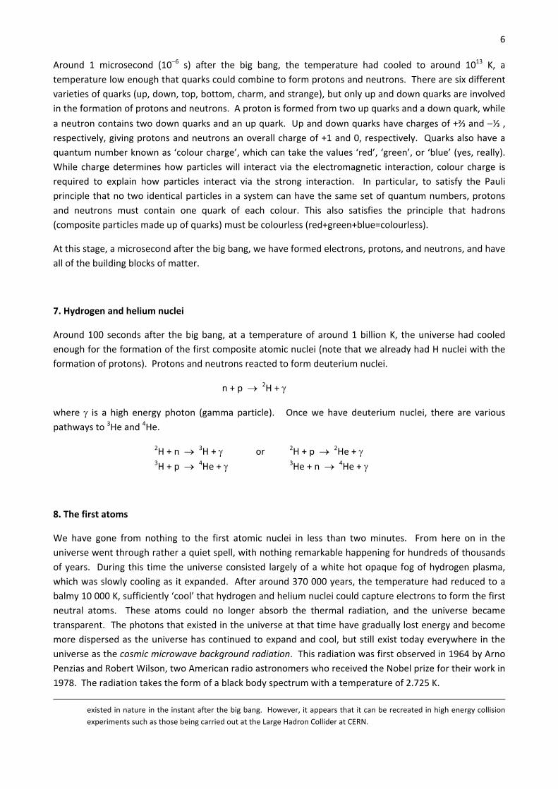
protons have sufficient energy to induce nuclear fusion. The star begins to shine. Two examples of star
forming regions or ‘stellar nurseries’ within large gas clouds are shown in the image below.
The first stars, known as Population III stars, were huge, hundreds of times heavier than our sun, and
burned out relatively quickly (compared to later stars), on a timescale of three to four million years5. For
most of their lifetime they were fuelled largely by hydrogen burning, a multi‐step process in which four 1H
nuclei are fused to form a single 4He nuclei and various other elementary particles. There are two different
mechanisms for hydrogen burning, but in young stars (including our sun) the proton‐proton cycle
dominates, and produces around 90% of the star’s energy.
1H + 1H 2H + e+ + e
2H + 1H 3He +
3He + 3He 4He + 21H
Once the supply of 1H in the core of a star was exhausted, near the end of its lifetime, the dominant process
became helium burning, the fusion of two 4He nuclei to form a 8Be nucleus.
4 It is thought that molecular hydrogen also formed at this stage via gas‐phase reactions, and that the presence of H2 was important in driving the gravitational collapse that led to formation of the first stars. In the modern universe, H2 formation is dominated by chemistry occurring on the surface of interstellar dust grains, with gas‐phase processes making only a very small contribution. 5 Somewhat counterintuitively, more massive stars have shorter lifetimes. Although the amount of fuel a star
has increases with mass, the rate at which it consumes this fuel increases even faster with mass. It is found
that a star’s lifetime on the main sequence (the period while it is burning hydrogen as fuel) is proportional to
1/m3.
8
4He + 4He 8Be +
The 8Be nucleus resulting from this process is not stable, and usually decays back to two 4He nuclei, but can
also undergo other reactions. For example,
8Be + 4He 12C +
From 12C it is possible to make all of the even numbered elements up to 56Fe through analogous nuclear
fusion process
12C + 4He 16O +
16O + 4He 20Ne +
20Ne + 4He 24Mg +
24Mg + 4He 28Si + and so on.
Odd numbered nuclei are formed in less efficient reactions involving proton capture. Many of the original
Population III stars probably didn’t get much further than helium burning before reaching the end of their
lifetime, at which point they exploded in supernovae, scattering the elements they had formed through
space. As far as we know, no Population III stars are still in existence. Over time, the cycle of giant gas
cloud formation and star formation was repeated to form a generation of Population II stars. The presence
of heavier elements in the gas clouds modified their cooling and contraction properties, with the result that
Population II stars tend to be smaller than the first generation of stars, with much longer lifetimes. Many
Population II stars are still in existence, and are thought to be between 10 and 13 billion years old (for
comparison, remember that the universe is thought to be around 13.8 billion years old). These stars have a
much higher fraction of ‘heavy’ (i.e. non hydrogen and helium) nuclei than the Population III stars. For
some Population II stars that have reached the end of their lives, the star formation cycle has repeated
itself to form Population I stars, with ages of less than 10 billion years, which contain even higher levels of
heavy nuclei, having been given a ‘head start’ by their ‘parent’ Population II stars. Our sun is a Population I
star. To keep things in perspective, even in so‐called ‘high metallicity’6 star such as the sun, only around
1.8% of nuclei within the sun are heavy elements.
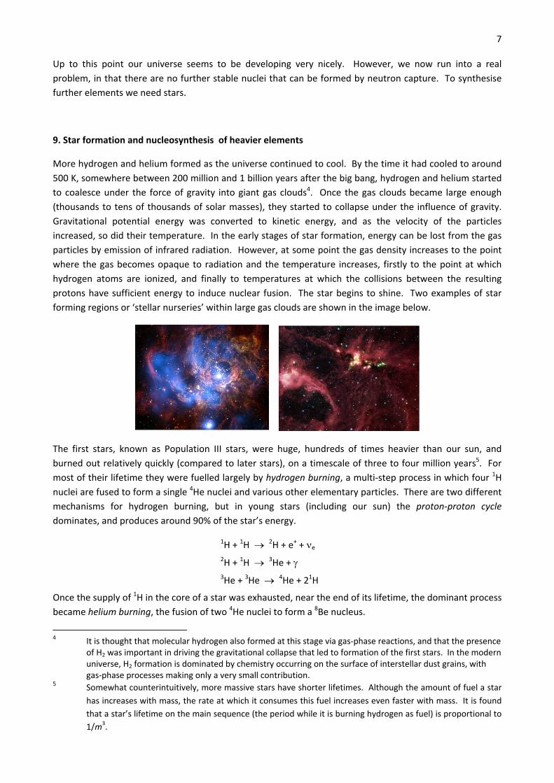
Nuclear fusion processes of the type described above are energetically favourable until we reach the 56Fe
nucleus. Iron has the most stable nucleus in terms of binding energy per nucleon, as shown in the plot
below.
Beyond 56Fe, fusion processes are no longer energetically favourable, and heavier elements are instead
built up gradually through a combination of neutron capture and decay (electron emission). In the
example below, 98Mo (atomic number 42) captures a neutron to form 99Mo, which then emits an electron
6 The metallicity of a star is the proportion of its matter made up from elements other than H and He.
9 to form 99Tc, with atomic number 43, and a neutrino. Neutron capture followed by electron emission
therefore has the overall effect of increasing the atomic number by one.
98Mo + n 99Mo +
99Mo 99Tc + e +
10. Dispersion of chemical elements
The dispersion of chemical elements from stars into the interstellar medium occurs at the end of a star’s
lifetime. The mechanism for the dispersion depends on the mass of the star.
During the time when a star is fuelled primarily by hydrogen burning it is known as a main sequence star.
For a star similar in size to our sun, this period lasts around 10 billion years. Once all the hydrogen in the
core has been converted to helium the hydrogen fusion reactions in the core stop. However, they continue
in the shell around the core. The core begins to cool and contract under gravity. Eventually, in a sequence
of processes similar to the formation of the original star, the core of the star has condensed and increased
in temperature to the point where the density and temperature are high enough to initiate helium burning.
The outer layers of the star begin to cool, expand, and shine less brightly, and the star is now a red giant.
Eventually the helium within the star’s core is converted to carbon, at which point the core becomes a
white dwarf, and the outer layers of the star drift away to form a gaseous shell called a planetary nebula.
The atomic species within the planetary nebula will eventually drift away into the interstellar medium.
Once nuclear fusion reactions stop completely, the core of the now dead star is known as a black dwarf.
The sequence of events unfolds rather differently for massive stars (3‐50 times heavier than our sun). Their
main sequence lifetimes are much shorter, at millions rather than billions of years. Once a massive star has
exhausted its supply of hydrogen and begins helium burning, it expands much more than a low mass star,
forming a red supergiant. Over the next million years, many different nuclear reactions occur in the core,
forming different elements in shells around an iron core. Eventually, the star runs out of fuel, leading to a
spectacular gravitational collapse and subsequent explosion called a supernova. In contrast to the millions
of years over which the star has evolved up to this point, the supernova event takes less than a second.
The resulting shock wave blows off the outer layers of the star into the interstellar medium, but sometimes
the core will survive the explosion. If the remaining core has a mass of between 1.5 and 3 solar masses it
will contract to form a very dense neutron star, while a higher‐mass core will contract to form a black hole.
11. Cosmic abundance of the elements
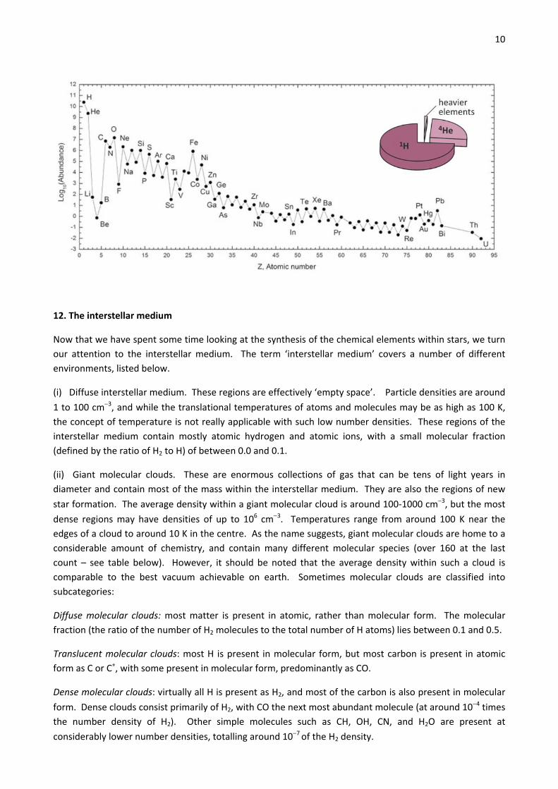
All of the chemical elements in the universe today formed through processes of the type described above.
The cosmic abundances of each element are plotted below (note the log scale), and show some interesting
features.
(i) The universe consists of around 74% hydrogen, 24% helium, and only 2% heavier elements.
(ii) The abundance falls off from light elements to heavier elements.
(iii) Iron has the most stable nucleus, and consequently is one of the most abundant elements.
(iv) Lithium, beryllium, and boron are extremely rare compared with other elements, since there is no
straightforward way to make them through nuclear reactions.
(v) Even elements are more abundant than odd since their nuclei are more stable and they are formed
more efficiently.
10
12. The interstellar medium
Now that we have spent some time looking at the synthesis of the chemical elements within stars, we turn
our attention to the interstellar medium. The term ‘interstellar medium’ covers a number of different
environments, listed below.
(i) Diffuse interstellar medium. These regions are effectively ‘empty space’. Particle densities are around
1 to 100 cm3, and while the translational temperatures of atoms and molecules may be as high as 100 K,
the concept of temperature is not really applicable with such low number densities. These regions of the
interstellar medium contain mostly atomic hydrogen and atomic ions, with a small molecular fraction
(defined by the ratio of H2 to H) of between 0.0 and 0.1.
(ii) Giant molecular clouds. These are enormous collections of gas that can be tens of light years in
diameter and contain most of the mass within the interstellar medium. They are also the regions of new
star formation. The average density within a giant molecular cloud is around 100‐1000 cm3, but the most
dense regions may have densities of up to 106 cm3. Temperatures range from around 100 K near the
edges of a cloud to around 10 K in the centre. As the name suggests, giant molecular clouds are home to a
considerable amount of chemistry, and contain many different molecular species (over 160 at the last
count – see table below). However, it should be noted that the average density within such a cloud is
comparable to the best vacuum achievable on earth. Sometimes molecular clouds are classified into
subcategories:
Diffuse molecular clouds: most matter is present in atomic, rather than molecular form. The molecular
fraction (the ratio of the number of H2 molecules to the total number of H atoms) lies between 0.1 and 0.5.
Translucent molecular clouds: most H is present in molecular form, but most carbon is present in atomic
form as C or C+, with some present in molecular form, predominantly as CO.
Dense molecular clouds: virtually all H is present as H2, and most of the carbon is also present in molecular
form. Dense clouds consist primarily of H2, with CO the next most abundant molecule (at around 104 times
the number density of H2). Other simple molecules such as CH, OH, CN, and H2O are present at
considerably lower number densities, totalling around 107 of the H2 density.
11 (iii) Circumstellar medium. These are the regions directly around a star, and the environment within these
regions depends on the type and extent of evolution of the star. Regions around young stars experience
high photon fluxes in the UV so that all molecules are photodissociated and photoionized (such regions are
sometimes referred to as photon‐dominated regions). Around older stars there may be significant dust,
leading to surface chemistry as well as scattered starlight.
We will focus our attention on giant molecular clouds. The atomic composition of these regions is
determined by the past history of nearby stars (see Sections 9 and 10), which eject processed nuclear
material via stellar winds and supernova explosions. As we shall see, the molecular composition reflects
the balance between chemical evolution via reactions, destruction of molecules by light from stars or by
cosmic rays, and condensation and subsequent reaction on dust grains.
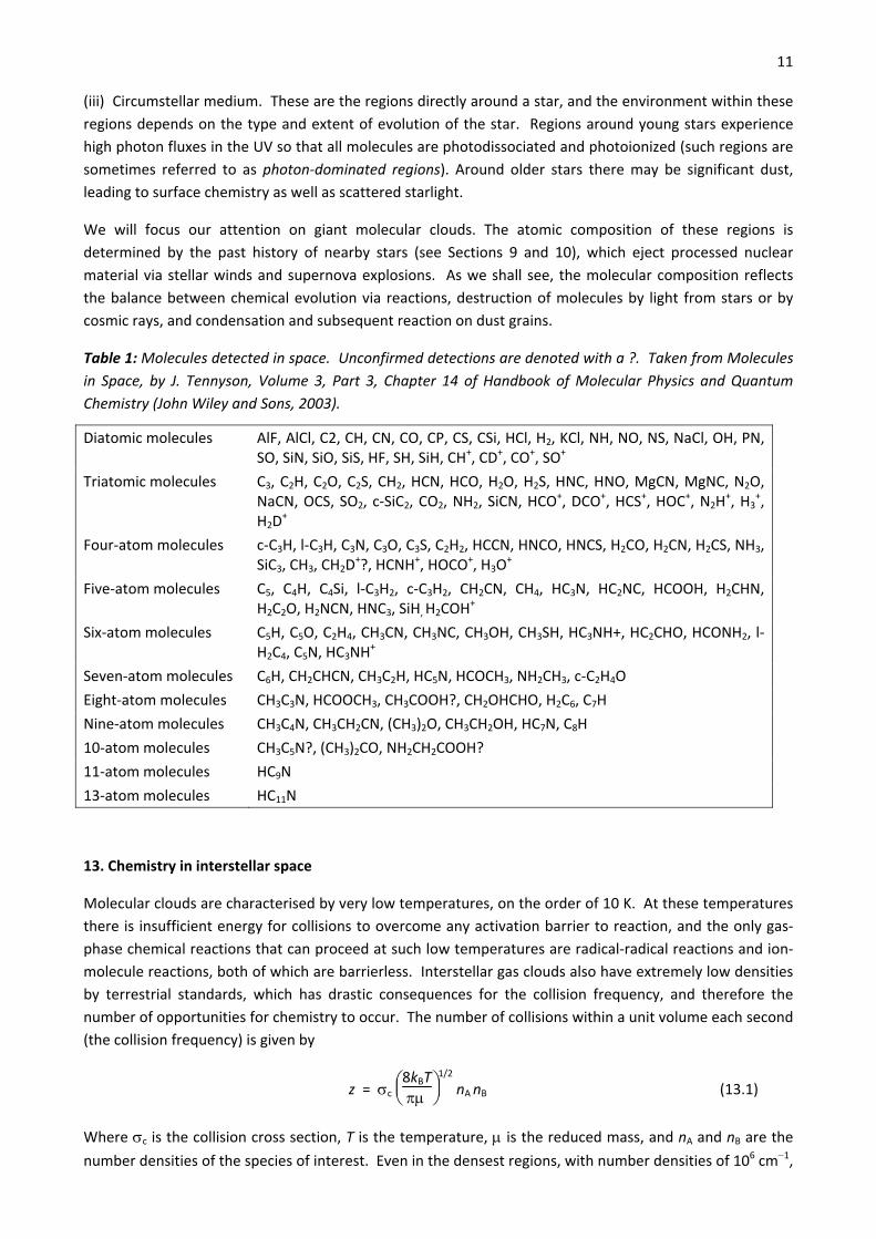
Table 1: Molecules detected in space. Unconfirmed detections are denoted with a ?. Taken from Molecules
in Space, by J. Tennyson, Volume 3, Part 3, Chapter 14 of Handbook of Molecular Physics and Quantum
Molecular clouds are characterised by very low temperatures, on the order of 10 K. At these temperatures
there is insufficient energy for collisions to overcome any activation barrier to reaction, and the only gas‐
phase chemical reactions that can proceed at such low temperatures are radical‐radical reactions and ion‐
molecule reactions, both of which are barrierless. Interstellar gas clouds also have extremely low densities
by terrestrial standards, which has drastic consequences for the collision frequency, and therefore the
number of opportunities for chemistry to occur. The number of collisions within a unit volume each second
(the collision frequency) is given by
z = c
8kBT
1/2
nA nB (13.1)
Where c is the collision cross section, T is the temperature, is the reduced mass, and nA and nB are the
number densities of the species of interest. Even in the densest regions, with number densities of 106 cm1,
12
collision rates are around 5 x 10⁴ s1, approximately one collision every half an hour. In less dense regions,
atoms and molecules may go for many weeks, or even longer, between collisions. Chemistry therefore
occurs at a very slow rate in interstellar space compared to the timescales we are used to on earth.
However, since giant molecular clouds last for around 10 to 100 million years before they are dissipated by
heat and stellar winds from stars forming within them, there is plenty of time for some quite complex
chemistry to occur, albeit at a rather leisurely rate. The very low collision frequency has important
consequences for the types of molecules that may form in interstellar space. As we can see from the table
of molecules above, terrestrial concepts of molecular stability simply do not apply in this extremely non‐
reactive environment. Carbon does not need to have four bonds; in fact, there are many subvalent species,
radicals, molecular ions and energetic isomers amongst the molecules observed in interstellar gas clouds.
Carbon‐containing compounds tend to be highly unsaturated, with many double and triple bonds, and few
branched chains. Polyynes are commonly observed, some with quite long chain lengths, for example
HCCCCCCCCCCCN. Many of the molecules observed in space would react almost instantly
were they transported to earth.
As noted above, collisions between atoms and molecules in interstellar space are extremely infrequent, and
as such, conventional chemical principles such as 'thermalisation' are not really relevant. It therefore
makes more sense to consider chemistry in the interstellar medium in terms of individual collisions. We
will return to this idea in detail when considering theoretical studies of astrochemical reactions later on in
the course.
14. Molecular synthesis in interstellar gas clouds
Gas‐phase molecular synthesis in interstellar clouds is believed to occur primarily via ion‐molecule
reactions, with some neutral reactions contributing. Since the molecular species identified from
spectroscopic data are mostly neutral, the ionic species formed in these processes must become charge‐
neutral relatively quickly. The general scheme of molecular synthesis therefore looks something like the
following:
Neutral gas ionization
Small ions reaction
Large ions neutralisation
Observed and ambient species
Chemistry can also occur on the surface of dust grains. Surface‐catalyzed reactions of this type turn out to
be very important in the interstellar medium, and we will look at these in some detail later.
We will now consider the types of reaction contributing to each of the three stages involved in gas‐phase
interstellar chemistry i.e. ionization, reaction, and neutralisation, before moving on to look at dust‐grain
catalysed chemistry.
15. Ionization processes in the interstellar medium
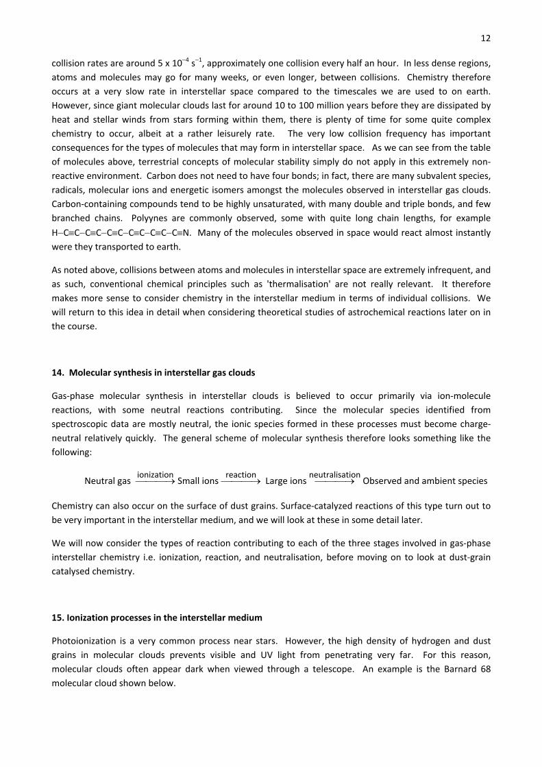
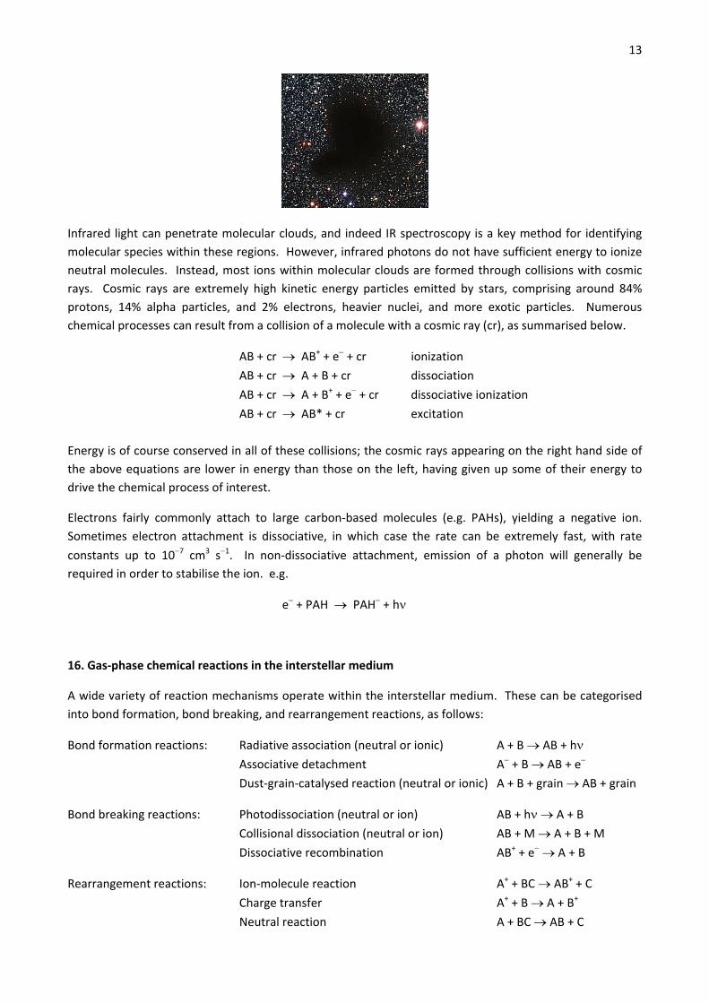
Photoionization is a very common process near stars. However, the high density of hydrogen and dust
grains in molecular clouds prevents visible and UV light from penetrating very far. For this reason,
molecular clouds often appear dark when viewed through a telescope. An example is the Barnard 68
molecular cloud shown below.
13
Infrared light can penetrate molecular clouds, and indeed IR spectroscopy is a key method for identifying
molecular species within these regions. However, infrared photons do not have sufficient energy to ionize
neutral molecules. Instead, most ions within molecular clouds are formed through collisions with cosmic
rays. Cosmic rays are extremely high kinetic energy particles emitted by stars, comprising around 84%
protons, 14% alpha particles, and 2% electrons, heavier nuclei, and more exotic particles. Numerous
chemical processes can result from a collision of a molecule with a cosmic ray (cr), as summarised below.
AB + cr AB+ + e + cr ionization
AB + cr A + B + cr dissociation
AB + cr A + B+ + e + cr dissociative ionization
AB + cr AB* + cr excitation
Energy is of course conserved in all of these collisions; the cosmic rays appearing on the right hand side of
the above equations are lower in energy than those on the left, having given up some of their energy to
drive the chemical process of interest.
Electrons fairly commonly attach to large carbon‐based molecules (e.g. PAHs), yielding a negative ion.
Sometimes electron attachment is dissociative, in which case the rate can be extremely fast, with rate
constants up to 107 cm3 s1. In non‐dissociative attachment, emission of a photon will generally be
required in order to stabilise the ion. e.g.
e + PAH PAH + h
16. Gas‐phase chemical reactions in the interstellar medium
A wide variety of reaction mechanisms operate within the interstellar medium. These can be categorised
into bond formation, bond breaking, and rearrangement reactions, as follows:
Bond formation reactions: Radiative association (neutral or ionic) A + B AB + h Associative detachment A + B AB + e
Dust‐grain‐catalysed reaction (neutral or ionic) A + B + grain AB + grain
Bond breaking reactions: Photodissociation (neutral or ion) AB + h A + B
Collisional dissociation (neutral or ion) AB + M A + B + M
Dissociative recombination AB+ + e A + B
Rearrangement reactions: Ion‐molecule reaction A+ + BC AB+ + C
Charge transfer A+ + B A + B+
Neutral reaction A + BC AB + C
14 Apart from photodissociation, these processes are all bimolecular, and usually diffusion controlled, with
rate constants of around 109 cm3 s1. The various types of reaction are considered in more detail and
illustrated with examples in the following.
16.1 Bond formation reactions
16.1.1 Radiative association
Conservation of energy and momentum mean that the product of an association reaction, in which two
reactants combine to form a single product, is usually highly internally excited. In terrestrial chemistry,
such reactions normally rely on a subsequent collision with a ‘third body’ in order to carry away some of
the energy of the excited product and thereby stabilize it. The low collision frequency in an interstellar gas
cloud rules out this pathway to stabilization, and instead the highly energised product either decays back to
reactants or is stabilised by emission of a photon. For example,
C+ + H2 CH2+* CH2
+ + h
CH3+ + H2O CH3
+.H2O + h CH3OH2+
If the product has an allowed electronic transition back to the ground state, then radiative association can
be very efficient; otherwise, it will be slow, relying on infrared emission to relax the excited molecule via
vibrational relaxation. Rate constants for radiative association vary from 1017 cm3 s1 for some diatomics
up to 109 cm3 s1 for polyatomics.
Radiative association reactions can rapidly build large ions in a single step. They are difficult to study in the
laboratory, and are often probed by studying the collisionally stabilised analogue.
16.1.2 Associative detachment
A negative ion and a neutral combine and the resulting negative ion detaches an electron. This type of
reaction is fairly common for small species, and is also thought to occur for larger ones.
e.g. OH + H H2O + e
16.1.3 Dust‐grain‐catalysed reactions
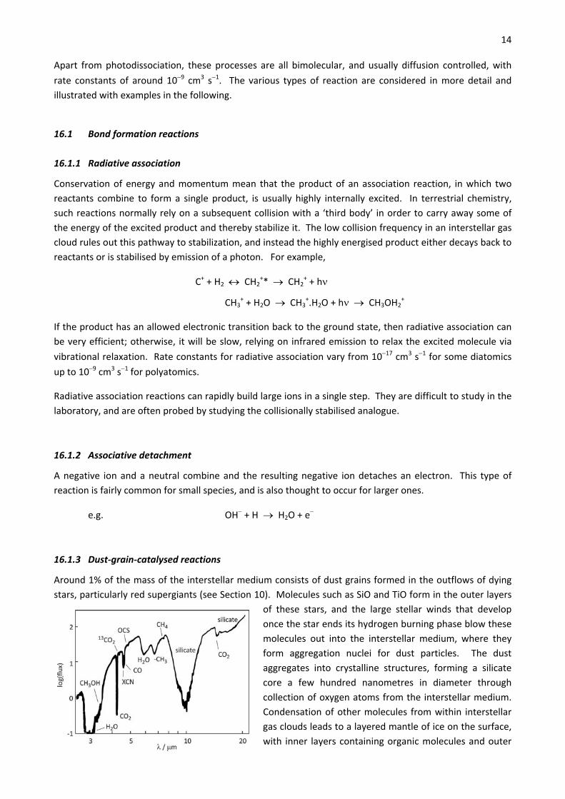
Around 1% of the mass of the interstellar medium consists of dust grains formed in the outflows of dying
stars, particularly red supergiants (see Section 10). Molecules such as SiO and TiO form in the outer layers
of these stars, and the large stellar winds that develop
once the star ends its hydrogen burning phase blow these
molecules out into the interstellar medium, where they
form aggregation nuclei for dust particles. The dust
aggregates into crystalline structures, forming a silicate
core a few hundred nanometres in diameter through
collection of oxygen atoms from the interstellar medium.
Condensation of other molecules from within interstellar
gas clouds leads to a layered mantle of ice on the surface,
with inner layers containing organic molecules and outer
15 layers containing molecules such as H2O, CO, CO2, methanol, H2CO, NH3, and so on. A spectrum of
interstellar dust (from the W33A dust‐embedded massive young star), with some of the identifiable
absorption features labelled, is shown on the left.
Dust grain chemistry is difficult to study, and is currently not well understood. However, the mechanisms
available for dust grains to catalyse reactions in space must be similar to those involved in surface catalysis
on earth. Dissociative adsorption to a surface yields highly reactive species and alternative reaction
pathways, allowing reactions to proceed much more quickly than they would in the gas phase. A reaction
of vital importance in the interstellar medium which is known to occur almost exclusively on the surface of
dust grains is the formation of H2 from two H atoms adsorbed to the surface.
H + H dust grain H2
Organic synthesis is also thought to occur on the surface of dust grains. Adsorption of CO to the surface of
a dust grain provides a carbon source to initiate such reactions. For example,
CO + H HCO
HCO + H H2CO
H2CO + H H3CO
H3CO + H CH3OH
16.2 Bond breaking reactions
16.2.1 Photodissociation and collisional dissociation
Both of these processes should be familiar to you from earlier chemistry courses. Absorption of a photon
or collision with a third body provides the energy required to break a chemical bond.
16.2.2 Dissociative recombination
As the name suggests, the ion combines with an electron to produce a high‐energy neutral. Since a ‘third
body’ collision to carry away the energy of the neutral is highly unlikely, the product fragments into smaller
neutral species. For example,
H3O+ + e OH + 2H + 1.3 eV 29%
OH + H2 + 5.7 eV 36%
H + H2O + 6.14 eV 5%
O + H + H2 + 1.4 eV 30%
Such processes can be extremely fast, with rate constants of up to 106 cm3 s1, significantly faster than ion‐
molecule reactions.
16.3 Rearrangement reactions
16.3.1 Charge transfer
Charge transfer involves the transfer of an electron from a neutral to an ion, and may lead to dissociation of
the resulting ion. The charge transfer often occurs at large separations of up to 10 Å, and the process has a
correspondingly large reaction cross section.
An example is the dissociative charge transfer from He+ to CO (electron transfer from CO to He+).
16
He+ + CO C+ + O + He + 2.2 eV
The large ionization energy of He (24.6 eV) is released during the charge transfer, leading to fragmentation
of the product CO+ back into its atomic constituents. This might seem like a backward step in terms of
molecular synthesis, but the C+ ion formed in this reaction can go on to react further.
16.3.2 Neutral reactions
Fewer neutral reactions are involved in the interstellar medium than ion‐molecule reactions, as they tend
to have activation barriers, but even reactions with barriers can be important in higher temperature
shocked regions; for example, when a supernova shock wave passes through a gas cloud then the gas is
compressed and can heat up to over 1000 K.
16.3.3 Ion‐molecule reactions
Ion‐molecule reactions are usually barrierless (though there can often be a centrifugal barrier – see Section
42) and make up the majority of bimolecular reactions occurring in the ISM. The charge‐transfer reactions
described in Section 16.3.1 are a subset of ion‐molecule reactions, but there are many other varieties. A
few examples are given below.
Hydrogen atom abstraction
H atom abstraction reactions are important due to the high abundance of H atoms in the interstellar
medium. One of the most common reactions is
H2 + H2+ H3
+ + H + 1.7 eV (fast)
This is a fast reaction due to the high abundance of both reactants. The H3+ ion is extremely important in
the ISM, being responsible for most of the proton transfer chemistry occurring.
Another example of a hydrogen atom abstraction is the reaction between NH3+ and H2.
NH3+ + H2 NH4
+ + H + 0.9 eV (slow)
This reaction occurs much more slowly, and has an interesting temperature dependence. The reaction
involves a barrier, such that the rate slows as the temperature is reduced from room temperature down to
around 70 K. At lower temperatures the rate increases again as a quantum tunnelling mechanism takes
over. Tunnelling becomes easier (and therefore faster) at lower temperatures since the collisions are
slower and the reactants spend more time in close proximity. Within molecular clouds, the reaction goes
almost entirely via the tunnelling mechanism.
Proton transfer
Proton transfer reactions are common from species of lower to higher proton affinity. The reaction
exoergicity can be determined by the difference in proton affinities (PA) for the species involved. The H3+
ion is commonly involved in such reactions. For example,
H3+ + H2O H3O
+ + H2 + 2.8 eV
In this case the exoergicity is E = PA(H2O) – PA(H2) = 2.8 eV.
17 Carbon insertion
Carbon insertion reactions involve the insertion of a C+ ion into a carbon chain. An atom or electron must
be ejected during the process in order to conserve momentum e.g.
C+ + C2H2 C3H+ + H + 2.2 eV
These reactions are important in synthesis of many of the carbon‐containing molecules in the ISM. As an
example, the C3H+ ion formed in the above reaction can go on to react further, eventually forming cyclic
C3H2 via a sequence of steps involving hydrogen abstraction and electron ion recombination.
C3H+ + H2 C3H2
+ + H
C3H2+ + e C3H2
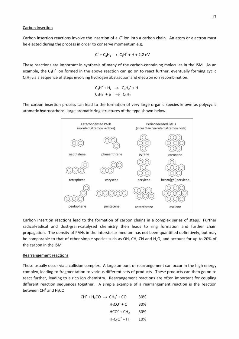
The carbon insertion process can lead to the formation of very large organic species known as polycyclic
aromatic hydrocarbons, large aromatic ring structures of the type shown below.
Carbon insertion reactions lead to the formation of carbon chains in a complex series of steps. Further
radical‐radical and dust‐grain‐catalysed chemistry then leads to ring formation and further chain
propagation. The density of PAHs in the interstellar medium has not been quantified definitively, but may
be comparable to that of other simple species such as OH, CH, CN and H2O, and account for up to 20% of
the carbon in the ISM.
Rearrangement reactions
These usually occur via a collision complex. A large amount of rearrangement can occur in the high energy
complex, leading to fragmentation to various different sets of products. These products can then go on to
react further, leading to a rich ion chemistry. Rearrangement reactions are often important for coupling
different reaction sequences together. A simple example of a rearrangement reaction is the reaction
between CH+ and H2CO.
CH+ + H2CO CH3+ + CO 30%
H3CO+ + C 30%
HCO+ + CH2 30%
H2C2O+ + H 10%
18 17. Neutralisation processes in the interstellar medium
As noted in Section 14, most of the molecules observed in the interstellar medium are neutral, while the
products of the ion‐molecule reactions discussed in the previous section are ionic. There are a number of
pathways by which an ion may be transformed into a neutral molecule within the interstellar medium. We
have already covered one of these. In electron‐ion dissociative recombination (Section 16.2.2), an ion and
electron combine to form a neutral, which then fragments into two or more neutral products. Similarly, a
negative ion and a positive ion may recombine to form a neutral complex, which dissociates into neutral
products.
Examples: CO+ + e C + O electron‐ion dissociative recombination
HCCCNH+ + e HCCCN + H / HCCNC + H electron‐ion dissociative recombination
O + O2+ O + O2 ion‐ion dissociative recombination
18. A simple model for calculating the rate of ion‐molecule reactions
State‐of‐the‐art QCT and quantum scattering calculations are capable of predicting reaction cross sections
and rate constants for ion‐molecule reactions. However, these calculations are only possible when a
detailed potential energy surface is available for the reaction under study, which is often not the case. In
the following, we will show how we can use basic principles of collision physics to understand the key
factors determining the rates of ion‐molecule reactions, and to develop a simple expression which can be
used to calculate approximate rate constants. The model we will derive is known as the Langevin model,
and is the simplest of a variety of capture theories that have been developed to describe the rates of ion‐
molecule reactions. Such models assume that reaction is governed by the long‐range part of the
interaction potential, a region that can be treated classically to a reasonable approximation. To develop
the Langevin model, we need to introduce the concepts of impact parameter, orbital angular momentum
and centrifugal barriers. These will already be familiar to anyone taking the Molecular Reaction Dynamics
option.
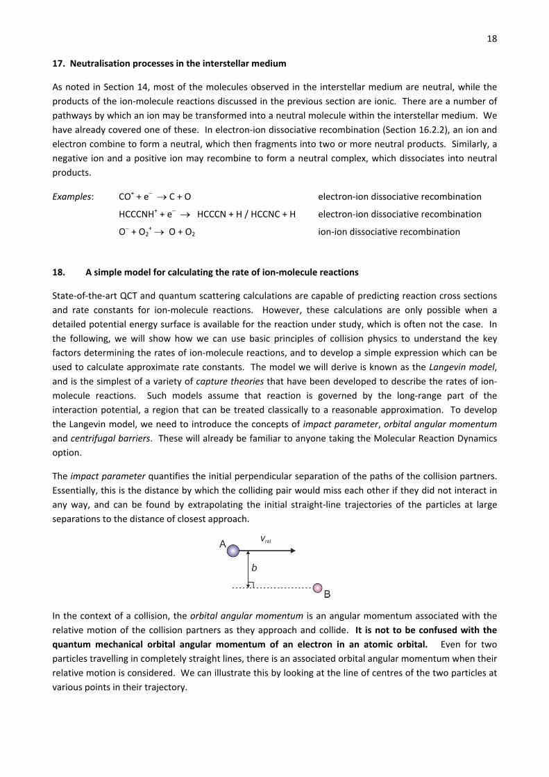
The impact parameter quantifies the initial perpendicular separation of the paths of the collision partners.
Essentially, this is the distance by which the colliding pair would miss each other if they did not interact in
any way, and can be found by extrapolating the initial straight‐line trajectories of the particles at large
separations to the distance of closest approach.
In the context of a collision, the orbital angular momentum is an angular momentum associated with the
relative motion of the collision partners as they approach and collide. It is not to be confused with the
quantum mechanical orbital angular momentum of an electron in an atomic orbital. Even for two
particles travelling in completely straight lines, there is an associated orbital angular momentum when their
relative motion is considered. We can illustrate this by looking at the line of centres of the two particles at
various points in their trajectory.
19
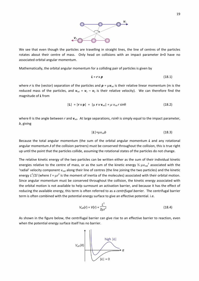
We see that even though the particles are travelling in straight lines, the line of centres of the particles
rotates about their centre of mass. Only head on collisions with an impact parameter b=0 have no
associated orbital angular momentum.
Mathematically, the orbital angular momentum for a colliding pair of particles is given by
L = r x p (18.1)
where r is the (vector) separation of the particles and p = vrel is their relative linear momentum (m is the
reduced mass of the particles, and vrel = v1 – v2 is their relative velocity). We can therefore find the
magnitude of L from
|L| = |r x p| = | r x vrel| = vrel r sin (18.2)
where is the angle between r and vrel. At large separations, rsin is simply equal to the impact parameter,
b, giving
|L|=vrelb (18.3)
Because the total angular momentum (the sum of the orbital angular momentum L and any rotational
angular momentum J of the collision partners) must be conserved throughout the collision, this is true right
up until the point that the particles collide, assuming the rotational states of the particles do not change.
The relative kinetic energy of the two particles can be written either as the sum of their individual kinetic
energies relative to the centre of mass, or as the sum of the kinetic energy ½ vrad2 associated with the ‘radial’ velocity component vrad along their line of centres (the line joining the two particles) and the kinetic
energy L2/2I (where I = r2 is the moment of inertia of the molecules) associated with their orbital motion.
Since angular momentum must be conserved throughout the collision, the kinetic energy associated with
the orbital motion is not available to help surmount an activation barrier, and because it has the effect of
reducing the available energy, this term is often referred to as a centrifugal barrier. The centrifugal barrier
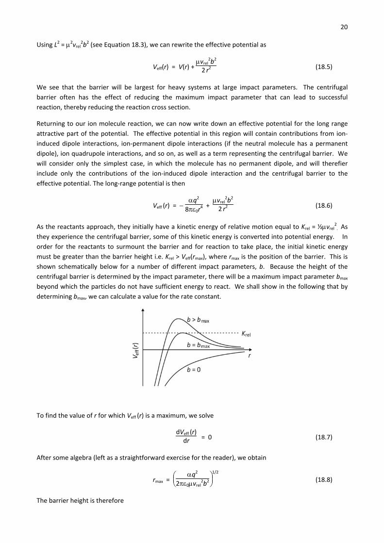
term is often combined with the potential energy surface to give an effective potential. i.e.
Veff(r) = V(r) + L2
2r2 (18.4)
As shown in the figure below, the centrifugal barrier can give rise to an effective barrier to reaction, even
when the potential energy surface itself has no barrier.
20
Using L2 = 2vrel2b2 (see Equation 18.3), we can rewrite the effective potential as
Veff(r) = V(r) + vrel2b2
2 r2 (18.5)
We see that the barrier will be largest for heavy systems at large impact parameters. The centrifugal
barrier often has the effect of reducing the maximum impact parameter that can lead to successful
reaction, thereby reducing the reaction cross section.
Returning to our ion molecule reaction, we can now write down an effective potential for the long range
attractive part of the potential. The effective potential in this region will contain contributions from ion‐
induced dipole interactions, ion‐permanent dipole interactions (if the neutral molecule has a permanent
dipole), ion quadrupole interactions, and so on, as well as a term representing the centrifugal barrier. We
will consider only the simplest case, in which the molecule has no permanent dipole, and will therefier
include only the contributions of the ion‐induced dipole interaction and the centrifugal barrier to the
effective potential. The long‐range potential is then
Veff (r) = q2
80r4 +
vrel2b2
2 r2 (18.6)
As the reactants approach, they initially have a kinetic energy of relative motion equal to Krel = ½vrel2. As they experience the centrifugal barrier, some of this kinetic energy is converted into potential energy. In
order for the reactants to surmount the barrier and for reaction to take place, the initial kinetic energy
must be greater than the barrier height i.e. Krel > Veff(rmax), where rmax is the position of the barrier. This is
shown schematically below for a number of different impact parameters, b. Because the height of the
centrifugal barrier is determined by the impact parameter, there will be a maximum impact parameter bmax
beyond which the particles do not have sufficient energy to react. We shall show in the following that by
determining bmax, we can calculate a value for the rate constant.
To find the value of r for which Veff (r) is a maximum, we solve
dVeff (r)dr = 0 (18.7)
After some algebra (left as a straightforward exercise for the reader), we obtain
rmax =
q2
20vrel2b21/2
(18.8)
The barrier height is therefore
21
Veff(rmax) = q2
80rmax4 +
vrel2b2
2rmax2
= 02vrel
4b4
2q2 (18.9)
For reaction to occur, we require Krel ≥ Veff(rmax). i.e.
12 vrel
2 ≥ 02vrel
4b4
2q2 (18.10)
Rearranging, we find that the maximum impact parameter for which reaction can occur is given by
b2 ≤
q2
0vrel21/2
(18.11)
The reaction cross section is then
r(vrel) = bmax2 =
q2
0vrel21/2
(18.12)
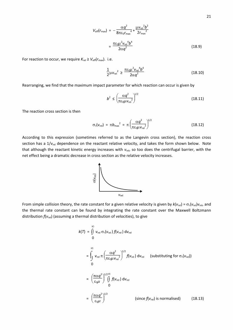
According to this expression (sometimes referred to as the Langevin cross section), the reaction cross
section has a 1/vrel dependence on the reactant relative velocity, and takes the form shown below. Note
that although the reactant kinetic energy increases with vrel, so too does the centrifugal barrier, with the
net effect being a dramatic decrease in cross section as the relative velocity increases.
From simple collision theory, the rate constant for a given relative velocity is given by k(vrel) = r(vrel)vrel, and
the thermal rate constant can be found by integrating the rate constant over the Maxwell Boltzmann
distribution f(vrel) (assuming a thermal distribution of velocities), to give
k(T) = 0
vrel r(vrel ) f(vrel ) dvrel
=
0
vrel
q2
0vrel21/2
f(vrel ) dvrel (substituting for r(vrel))
=
q2
0
1/2
0
f(vrel ) dvrel
=
q2
0
1/2
(since f(vrel) is normalised) (18.13)
22 Note that because we have only considered the possibility of a centrifugal barrier to reaction (i.e. we have
ignored any true barriers that may be present on the potential energy surface), this expression represents
an upper limit to the collisional rate coefficient for an ion‐molecule reaction. A key point to note is that the
thermal rate constant we have derived is independent of temperature, in line with our previous discussion
of ion‐molecule reactions.
There are many more sophisticated models available for modelling ion‐molecule reaction rates. These
include quantum mechanical models such as the catchily named adiabatic capture and centrifugal sudden
approximation (ACCSA) theory, which takes into account the rotational states of the reactants, variational
transition state theory, and trajectory calculations. The latter two approaches require a reasonably
detailed knowledge of the potential energy surface for the reaction. Variational transition state theory is
an improved version of transition state theory, which you have met in statistical mechanics courses.
Trajectory calculations are covered in the Molecular Reaction Dynamics option.
19. Laboratory‐based astrochemistry
While astronomical observations provide raw data on the physical conditions in various regions of space
and the atomic and molecular species present, interpreting such data is only possible as a result of
laboratory‐based studies of a wide range of basic atomic and molecular processes. For example, molecular
identification via the assignment of spectral lines recorded using a telescope can only be achieved through
comparison with spectra recorded on earth (if the molecule of interest is sufficiently stable and can be
generated in sufficiently high quantities to detect) or spectra simulated on the basis of electronic structure
calculations. Kinetic models of interstellar chemistry require knowledge of rate constants for individual
chemical steps, which again must either be measured in a laboratory or modelled theoretically.
Understanding the complex chemistry occurring on the surface of interstellar dust grains requires the
development of suitable laboratory‐based analogues and methods for studying them. In many cases, the
much higher number densities involved in laboratory experiments, combined with the extremely high
detection sensitivities achievable for a wide range of molecules of interest, mean that it is often possible to
simulate processes that occur over millions of years in space within a few minutes in the laboratory.
Laboratory‐based astrochemistry is a growing field, and an ideal playground for physical chemists. In the
following, we will outline a few of the current challenges in astrochemistry that laboratory‐based studies
can help to address.
19. The grand challenge: chemical modelling of giant molecular clouds
Perhaps the ultimate goal of the astrochemistry community is to develop a complete chemical model of an
interstellar gas cloud. Amongst other things, such models would allow the age of a molecular cloud to be
estimated based on measurements of its atomic composition.
The techniques used to model molecular clouds are very similar to those developed for modelling chemical
processes in the earth’s atmosphere. However, there are many more unknowns in modelling interstellar
gas clouds than in atmospheric models. Many of the rate constants, particularly for reactions occurring on
dust grains, are unknown, and measurements on gas clouds to establish parameters such as temperature
and number density cannot be carried out directly in the same way as they can in the earth’s atmosphere.
Nonetheless, the process of setting up and solving a kinetic model follows the same general principles as
for an atmospheric model, and similar parameters need to be quantified:
23 (i) Data on the chemical composition of the cloud is taken from experimental observations. Ideally,
we would have accurate number densities for all chemical species within the cloud, including
electrons.
(ii) The physical conditions within the cloud are needed, including temperature, number density,
electron temperature, radiation field, and extinction coefficient (used to estimate the dust
composition). These conditions will not generally be constant throughout the cloud. For example,
the density will fluctuate due to stellar winds, stellar explosions such as supernovae, and random
perturbations, while the temperature is determined by the balance of heat inputs from radiation
and exothermic chemical reactions, and heat losses, primarily radiative losses accompanying
relaxation of atomic and molecular species from excited states. The radiation field is determined
by the proximity to nearby stars and extinction by interstellar dust.
(iii) Transport processes must be considered. These include diffusion and collisions, as well as more
exotic phenomena such as shock fronts transiting the clouds, and magnetic turbulence.
(iv) An estimate of the radiation field emanating from newly forming stars within the cloud is important
in order to account for photochemical processes occurring in these regions.
(v) Accurate reaction rates for all chemical processes occurring in the cloud are needed. Often these
are not known, and must be estimated or modelled.
(vi) The reactions to be included in the model must be decided upon, along with the target species that
will be compared with available experimental data.
Once all of the required parameters have been quantified, we can set up the rate equations, a set of
coupled differential equations, and propagate them numerically in time to predict the concentrations of
the target species. Some parameters, for example the chemical composition of the cloud and sometimes
the temperature in different regions, can be determined from astronomical observation data (see Sections
2 to 4) in combination with data from quantum chemistry calculations. Other parameters, such as rate
constants, must be determined in laboratory‐based studies, either through experimental measurement or
theoretical modelling.
In addition to the 'grand challenge' of developing a complete chemical model of an interstellar gas cloud, a
number of more specific problems in astrochemistry are currently attracting considerable attention from
the research community. Two examples are given in the following.
20. The search for biological molecules
There is an enormous amount of interest in detecting biological molecules in interstellar space, as their
presence would represent a significant step in the search for extraterrestrial life as well as potentially
providing insight into the origins of life on earth. Laboratory‐based studies appear to indicate that there
are feasible mechanisms for generating simple amino acids under the conditions known to be present
within interstellar gas clouds, and that glycine (the simplest amino acid) and perhaps other biogenic
molecules should be abundant enough to be detected. However, to date there has only been one reported
detection of glycine7, and this has been contested rather than confirmed8.
7 Y‐J Kuan, S. B. Charnley, H‐C. Huang, W‐0L. Tseng, and Z. Kisiel, Interstellar glycine, Astrophys. J., 593, 848‐867
(2003).
24 21. The diffuse interstellar bands (DIBs)
The set of absorption features known as the diffuse interstellar bands represents perhaps the longest‐
standing mystery in astronomical spectroscopy. The first of these bands were reported in 19229, and now
number more than 400, ranging across the UV, visible, and infrared parts of the spectrum. Despite general
agreement that the absorptions are mostly likely due to large organic molecules in the ISM, there have
been no definitive assignments to date. PAHs (see Section 16.3.3), carbon chains, and fullerenes have all
been implicated as possible candidates for diffuse interstellar band absorptions. However, the
spectroscopy of these species is difficult to study in the laboratory and challenging to model accurately via
electronic structure calculations. It is known from solid‐state studies that PAH cations comprising 30 or
more carbon atoms absorb strongly in the visible, while the corresponding neutrals absorb in the UV, but
such large species are very difficult to generate and maintain in the gas phase, a requirement if high‐
resolution spectroscopic studies are to be performed.
While the IR emission bands arising from vibrational transitions of PAHs are fairly similar, the
electronic spectra are known to be highly characteristic for each molecule. If the problems outlined above
are overcome and laboratory‐based spectra for large PAHs become available, they are likely to allow
specific molecules to be identified within the ISM.
22. Overview of astrochemistry
This course has provided a brief overview of the types of chemical processes occurring in interstellar space,
beginning with the synthesis of chemical elements within stars and continuing with a summary of the
various processes that lead to the formation of complex molecules within interstellar gas clouds. We have
also considered a range of theoretical and experimental methods that may be employed to help identify
molecules in space and to unravel the chemical processes by which they are formed.
There is a great deal more to the field of astrochemistry. We have not even touched upon the chemistry
and physics of meteorites and comets, or the events leading to the formation of planets and their
subsequent chemistry. Astrochemistry is a fascinating and rapidly evolving field, in which physical chemists
have a great deal to offer, in the interpretation of observational data through our knowledge of
spectroscopy, in the kinetic modelling of reaction cycles, and in laboratory measurements of rate constants
and investigations into reaction mechanisms.
8 L. E. Snyder, F. J. Lovas, J. M. Hollis, D. N. Friedel, P. R. Jewell et al., A rigorous attempt to verify interstellar glycine, Astrophys. J., 619, 914‐30 (2005). 9 M. L. Heger, further study of the sodium lines in class B stars; the spectra of certain class B stars in the regions 5630 A – 6680 A and 3280 A to 3380 A; Note on the spectrum of g Cassiopeiae between 5860 A and 6600 A. Lick Observatory Bull., 337, 141‐148, (1922).