13
technical monograph 32 Fundamentals of Closed Loop Control Floyd D. Jury
| Date post: | 14-Apr-2018 |
| Category: |
Documents |
| Upload: | sergio-mario-herreros |
| View: | 236 times |
| Download: | 0 times |

7/27/2019 Fundamentals of Closed Loop Control
http://slidepdf.com/reader/full/fundamentals-of-closed-loop-control 1/12
technical
monograph32
Fundamentals of Closed
Loop Control
Floyd D. Jury
7/27/2019 Fundamentals of Closed Loop Control
http://slidepdf.com/reader/full/fundamentals-of-closed-loop-control 2/12
2
Fundamentals of
Closed Loop Control
Closed loop control is primarily a concept orphilosophy that is independent of the technology
required to implement it. An individual can become asdeeply involved in the mathematics as desired, but thefundamentals of closed loop control are relatively easyto understand and are essential in the building,operating, or maintaining of any control system. Thispaper not only discusses these fundamentals buttouches briefly on the technology involved.
The Process
The process is the prime component of the system. Itis the only reason for the system’s existence. Within
the context of this paper, a process is broadly definedas the system element, or component that is beingcontrolled. It is that which exists before any hardwareis added to measure or control. Many processesoperate sufficiently well without the addition of anycontrol equipment. When operated in this manner, thesystem is called an open loop control system. This willbe discussed further in the next section.
In many other practical situations, closed loop controlis required to achieve the desired performance fromthe system. The following is a partial list of typicalindustrial processes that frequently use closed loopcontrol.
1. Liquid level in a vessel
2. Pressure in a pipe or vessel
3. Flow through a piping system
4. Fluid temperature
5. Nuclear or chemical reaction rate
6. Fluid mixing ratio (concentration)
7. Turbine speed
When studying the overall control system, the processis simply treated as one of the elements in the controlloop. A complete description of the process requires a
knowledge of such things as the fluid properties andservice conditions, vessel or pipeline geometry,chemical or nuclear reaction dynamics, physicaldynamics of the device, or any other characteristic thatrelates changes in the process environment tochanges in the process variable of interest.
For the process, as well as all other elements in acontrol loop, an input and an output can be defined.Definition of the input and output depends upon howthe process is used. Input is that which normally
influences the status or condition of the process. Thisis frequently the load disturbance to the process. As a
result of this input influence on the process, aparameter of interest would normally be expected tochange in some predictable way. The parameter thatchanges is known as the output. The process output isnormally the variable that is to be controlled.
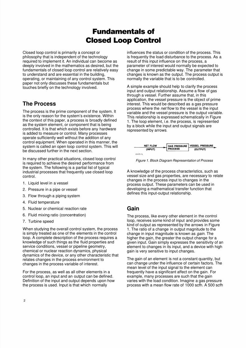
A simple example should help to clarify the processinput and output relationship. Assume a flow of gasthrough a vessel. Further assume that, in thisapplication, the vessel pressure is the object of primeinterest. This would be described as a gas pressureprocess where the net flow to the vessel is the inputvariable and the vessel pressure is the output variable.This relationship is expressed schematically in Figure
1. The loop element, i.e. the process, is representedby a block while the input and output signals arerepresented by arrows.
Figure 1. Block Diagram Representation of Process
A1470 / IL
A knowledge of the process characteristics, such asvessel size and gas properties, are necessary to relatechanges in the process input to changes in theprocess output. These parameters can be used indeveloping a mathematical transfer function thatdefines this input-output relationship.
Gain
The process, like every other element in the controlloop, receives some kind of input and provides somekind of output as represented by the arrows in Figure1. The ratio of a change in output magnitude to thechange in input magnitude is known as gain. Thehigher the gain, the greater the output change for a
given input. Gain simply expresses the sensitivity of anelement to changes in its input, and a device with highgain is very sensitive to input changes.
The gain of an element is not a constant quantity, butcan change under the influence of certain factors. Themean level of the input signal to the element canfrequently have a significant affect on the gain. Forexample, many processes are such that the gainvaries with the load condition. Imagine a gas pressureprocess with a mean flow rate of 1000 scfh. A 500 scfh

7/27/2019 Fundamentals of Closed Loop Control
http://slidepdf.com/reader/full/fundamentals-of-closed-loop-control 3/12
3
Figure 2. Typical Frequency Response Diagram
A1471 / IL
increase in the net flow rate would represent asignificant change and would undoubtedly cause alarge change in the process pressure. Now considerthe same process with a mean flow rate of 100,000scfh. In this case, the same 500 scfh net change inflow rate would cause only a minor change in theprocess pressure. As the system flow increases, thesystem pressure becomes less sensitive to the same
change in net flow, i.e. the process gain decreaseswith increasing load flow.
Without resorting to a rigorous mathematical proof, thisexample gives an intuitive feel for why the gain of aprocess can vary with the load on the system.Depending upon the type of process, the gain maydecrease, increase, or even remain constant withrespect to the operating point.
The frequency of the input signal can also have asignificant influence upon the gain of the element. This
is a phenomenon that is quite familiar to the hi-fi orstereo music buff. Every physical element, just like thestereo amplifier, can respond faithfully to relatively lowfrequency input signals, but as the frequencyincreases, a point is reached where the device can nolonger keep up with the demands placed on it. Pastthis point, the gain of the element normally decreasesrapidly with increasing frequency. In other words, thedevice becomes less sensitive to input changes as thefrequency increases beyond a certain point. Just priorto this frequency however, the element mayexperience a type of resonant condition and becomeeven more sensitive to input changes at a particularfrequency or band of frequencies.
A graph showing how the gain of an element respondsat various frequencies is known as a frequencyresponse diagram or Bode diagram. Actually, afrequency response diagram contains moreinformation than just the gain variation with frequency,but that is all we are interested in at this point. Thefrequency response diagram for a typical element isshown in Figure 2.
Open Loop Control
The simplest form of process control is known as openloop control, and in simple terms, open loop controlmeans that there is no direct measurement of thecontrolled variable available for use in makingcompensating adjustments to the input of the system.
This principle is illustrated in Figure 3.
Figure 3. Open Loop Pressure Control
A1472 / IL
Gas is drawn from the source pressure (P1) and fed to
the process vessel through a valve which is controlledby adjusting the actuator loading pressure (PL). Thepurpose of this system is to maintain the vesselpressure (P2) relatively constant while supplying thedownstream load with the gas flow that it requires tooperate properly. The downstream load may beanything from a burner to a large distribution network.
If the load flow is known and is constant, it is a simplematter to adjust the loading pressure so that the flowthrough the control valve will match that through theload valve. If these two flows are exactly matchedthere will be no variation in the vessel pressure;however, if they are not or if flow through either valve
tends to shift slowly with time, there will be a long termdrift of P2.
Indeed, this is one of the inherent disadvantages ofopen loop control. If the load flow changes in apredictable way, the loading pressure (PL) can bevaried accordingly to compensate for the load change.Unpredictable changes in the load flow will not becompensated for by the control valve and the vesselpressure will fluctuate.
However, there are advantages to open loop control,including low cost, simplicity, reliability, and inherentstability of most processes. Generally, disturbances or
changes to an open loop system do not cause it to gointo a state of self-sustaining oscillation; however,there are some processes, such as those involvingexothermic reactions, that are inherently unstable andrequire closed loop control to maintain stability.
Block Diagrams
A useful study of control systems would be difficultwithout the aid of block diagrams. A rather limited view

7/27/2019 Fundamentals of Closed Loop Control
http://slidepdf.com/reader/full/fundamentals-of-closed-loop-control 4/12
4
of the block diagram was introduced in Figure 1. Aparticular element in the system was defined andrepresented schematically by a block that had oneinput and one output. The input and Output wererepresented by arrows leading into and out of theblock. These arrows are referred to as input andoutput signals since they only represent information
about input influences and output responses ratherthan an actual physical flow of material. The blockshown in Figure 1 represents only the process.Referencing this to Figure 3, the process isrepresented by the pressure vessel and all theconnecting piping from the control valve to the loadvalve.
In Figure 1, notice that the process input is the net flow. The net flow consists of two components, theload flow and the control valve flow. These twocomponents are combined with the aid of a summing
junction, in Figure 4, to produce the net flow signal.
Figure 4. Block Diagram Summing Junction
A1473 / IL
The summing junction is simply a graphical techniquefor algebraically combining two or more signals in ablock diagram. A summing junction always has onlyone output signal which is the algebraic sum of all theinput signals. Each input has an associated algebraic
sign. If no signal is shown, it is normally assumed tobe positive.
The valve flow shown in Figure 4 is a result of theactuator positioning the valve to some specific travelposition (x). The actuator, in turn, operates under theinfluence of the loading pressure (PL). Figure 5 showshow the valve and actuator can be added to thecombination of Figure 1 and Figure 4 to produce ablock diagram that represents the open loop pressurecontrol system in Figure 3.
Figure 5. Block Diagram of Figure 3
A1474 / IL
The block diagram presents a simple, graphical meansto keep track of the various elements in the systemand their relationship to each other.
Closing the Loop
The simple, open loop control system il lustrated inFigures 3 and 5 performs quite satisfactorily in a widevariety of applications; however, it has certainlimitations that render it unacceptable in many othersituations. Long term drift may be a problem. Frequent
load fluctuations can occur, requiring nearly constantattention by an operator to adjust the actuator loadingpressure. The operator must intervene to manuallyclose the loop. The quality of control may vary fromone operator to the next, or the quality of control maybe poorer than desired when an operator isunavailable. All of these factors, among others, led tothe technique of letting the control system operateitself, i.e. automatically closing the loop.
Closing the loop means that the system is providedwith a way to measure the controlled variable,determine if a deviation from the desired value exists,and automatically provide whatever corrective
adjustment is needed for the actuator loadingpressure.
One of the simplest forms of closed loop control is theself operated pressure regulator. Self operated meansthat the energy required to operate the control valvecomes from within the system. For the system shownin Figure 3 the process pressure (P2) can be used toprovide the actuator loading pressure (PL) as indicatedin Figure 6. If the control valve allows more flow intothe system than the load valve removes, P2 will rise.This in turn will close the control valve, reducing theamount of flow into the system until it matches theoutflow. On the other hand, if the control valve allows
too little flow into the system, P2 will decrease allowingthe control valve to open and admit more flow.
Figure 6. Closed Loop, Self Operated,Gas Pressure Control System
A14745/ IL
Feedback action from the controlled pressure to theactuator will close the control valve if it is too far openand will open the valve if it is too far closed. This typeof compensating action is known as negativefeedback, and in a practical sense, simply means thatthe action of the corrective feedback is always suchthat it will try to prevent, or reduce, any change in thecontrolled variable.

7/27/2019 Fundamentals of Closed Loop Control
http://slidepdf.com/reader/full/fundamentals-of-closed-loop-control 5/12
5
In Figure 6, notice that the controlled pressure (P2)acts against the actuator diaphragm to produce a forcethat must be balanced by the spring in order tomaintain the valve at any flow opening. Because of thespring compression, more pressure is required on thediaphragm when the valve is closed than when thevalve is open. This means that as the load flow
increases, the control valve must open wider; and thecontrolled pressure, which acts on the diaphragm,must decrease to allow the valve to open. Thisdecrease in controlled pressure with load flow is calledoffset. In the gas industry, the offset resulting from ano-load to a full-load change is frequently referred toas droop.
Since the decrease in P2 is what opens the controlvalve to pass the increased flow, this decrease will beproportional to the load flow that exists. This gives riseto the name, proportional control. The amount ofchange that occurs in the measured variable (i.e. P
2 in
this case) as the system goes from a low load flowcondition to a maximum load flow condition is knownas the proportional band of the system. In the systemof Figure 6, the proportional band is a fixed quantitythat depends on the spring stiffness, the diaphragmarea, and the valve travel.
In addition to the spring compression which occursdue to valve travel, there is normally some initialcompression applied even when the valve is wideopen. This initial compression adjustment is normallymade by means of a screw thread arrangement on the
spring seat. The greater the initial compression appliedto the spring, the higher the pressure (P2) needed tohold the valve in any given position. This does notaffect the amount of droop or the proportional band ofthe system, but it does provide a means for adjustingthe range of pressures in which P2 will operate. Byadjusting the initial compression, the controlledpressure can be set to any desired point at any givenflow condition. This desired value of the controlledpressure is called the set point. In a gas pressureregulation system the set point is normally adjusted atthe low load flow. At higher load flows the controlledpressure will droop by some proportional amount.
The block diagram of Figure 5 can be easily modifiedto represent the closed loop system of Figure 6. Theloop is closed by connecting the process pressure (P2)arrow to the loading pressure (PL) arrow as indicatedin Figure 7.
Figure 7. Block Diagram of the Closed Loop System in Figure 6
A1476 / IL
The process is in the forward path of the control loop,while the valve and actuator comprise the feedbackpath. The negative sign indicates that the valve flowcompensates for changes in load flow to reducechanges in P2. Considering the closed loop system asa whole, the load flow is the system input and thecontrolled pressure (P2) is the system output.
System StabilityClosed loop control overcomes most of thedisadvantages of open loop control and provides moreaccurate and consistent control; however, closed loopcontrol introduces the possibility of loop instability.
The purpose of the control loop in Figure 7 is tomaintain the controlled variable at its desired value atall times desired changes in the load. If a deviation ofthe controlled variable should occur, the system willsense it and provide a corrective feedback actionaround the loop, i.e. from the controlled variable,through the actuator, valve, and process back again tothe controlled variable. Obviously, the more sensitive
this control loop is, the greater the correction and thebetter the performance. This is just another way ofsaying that high loop gain, or loop sensitivity, isneeded for good system performance.
The sensitivity of the loop is determined by thesensitivity of each element in the loop. If the gain ofany element is changed, the loop gain changes by thesame factor. The total loop gain is determined bymultiplying together the gains of all the elements in theloop. Steady-state accuracy, dynamic performance,and a number of other important performanceparameters are directly related to loop gain. Providedthat loop stability is maintained, all of these
performance parameters can be improved with higherloop gain.
If the loop gain is too high, however, the loop will beoverly sensitive and will have a tendency to oscillate.As the loop gain increases, the loop will become moreoscillatory and disturbances will take longer to die out.

7/27/2019 Fundamentals of Closed Loop Control
http://slidepdf.com/reader/full/fundamentals-of-closed-loop-control 6/12
6
Finally, a loop gain will be reached where thedisturbances will never die out and the loop willcontinually oscillate. This condition is known variouslyas instability, hunting, buzzing, or oscillation. Thecontrol loop, like many other physical systems, has acharacteristic frequency at which it oscillates whendisturbed. The physical parameters of the system
determine this characteristic cycling frequency. Inorder to maintain loop stability, the gain, or sensitivity,of the loop must be sufficiently low at this criticalfrequency.
The gain of the various elements in the loop can berelated quantitatively to the performance of the systemas well as to its stability. Consider the case of twoelements in series, as in the feedback path of Figure 7.These series elements can be considered as a singleunit by multiplying the series gains together. Figure 8shows how the actuator and valve can be combinedinto a single function represented by (H). Theelements of the forward path, in this case just the
process, can be represented by the function (G).
Figure 8. Generalized Version of a Closed Loop,Negative Feedback Control System
A1477 / IL
Figure 8 can be used to represent any closed loop,
negative feedback control system. It can be used toderive a simple mathematical relationship that helps inunderstanding the system performance. Rememberingthe definition of a summing junction, a formula can bewritten to describe its output.
W n+ W L*W v (1)
Now recall the definition of gain as the ratio of outputto input. Utilizing this definition, the output of anyelement can be written as the product of the inputtimes the gain of the element.
W v+ HP 2 (2)
P 2+ GW n (3)
Equation (2) can be substituted into Equation (1) toeliminate Wv.
W n+ W L* HP 2 (4)
Equation (4) can be substituted into Equation (3) toeliminate Wn.
P 2+ G(W L* HP 2) (5)
Equation (5) can now be rearranged in severalalgebraic steps to a more useful form.
P 2+ GW L*GHP 2
P 2)GHP 2+ GW L
P 2(1)GH )+ GW L
P 2ńW L+ Gń(1)GH ) (6)
(Since (P 2 /W L ) is the ratio of the system output to thesystem input, Equation (6) represents the gain of theentire closed loop system. Since the sensitivity of theoutput (P2) to changes in load (WL) should be as lowas possible, the magnitude of the expression on theright side of Equation (6) should be as small aspossible. This is accomplished by keeping the loop
gain (GH) as high as possible. If the loop gain (GH) isrelatively high, the one in the denominator can besafely neglected and Equation (6) reduces to Equation(7).
P 2ńW L[ 1ń H (7)
Equation (7) illustrates an important principle of closedloop control. When negative feedback is employedaround a process, or any other element, and high loopgain is maintained, the response of the total closedloop is essentially independent of the processcharacteristics (G). If there is any non-linearity or other
irregularity in the forward path of the loop, it caneffectively be eliminated by the high loop gain andnegative feedback.
It should be obvious that high loop gain is the way toachieve good system performance, but as it hasalready been pointed out, too high a loop gain canlead to loop instability. The loop as it has been definedso far in Figure 7 has no flexibility in terms of gainadjustment to alter the characteristics of the system.
The ControllerThe addition of a controller to the loop can greatlyimprove the quality of control and can provide theflexibility needed to adjust the loop gain to match therequirements of the system.
The controller shown in Figure 9 performs three basicfunctions. It senses the controlled variable (P2),compares it to the desired set point value, andprovides an output to operate the actuator.

7/27/2019 Fundamentals of Closed Loop Control
http://slidepdf.com/reader/full/fundamentals-of-closed-loop-control 7/12
7
Figure 9. Typical Closed Loop with Controller
A1478 / IL
The gain of the controller is easily adjustable oversome wide range of values. This gain adjustment issometimes referred to as the proportional bandadjustment. Narrowing the proportional band is thesame as increasing the gain. A narrower proportionalband means that less input to the controller is neededto provide full output, thus the controller is moresensitive to changes in its input signal.
Since the controller is now one of the elements in theloop, changing the gain of the controller will changethe loop gain by the same factor. Adjusting theproportional band, or gain, of the controller allows theoperator to achieve the best high gain performanceconsistent with loop stability. Frequently, the operatormust compromise and accept poorer control thandesired in order to maintain a stable loop.
The simplest type of controller is the proportionalcontroller which has a single gain, or proportionalband, adjustment. This controller has only a singlemode of operation. If the gain is reduced so that theloop becomes less sensitive at the critical frequency,
stability is maintained; but both steady-state accuracyand transient performance suffer due to reduced gainat the high and low frequencies.
Sometimes a two-mode controller, calledproportional-plus-reset, is used to improve thesteady-state accuracy. By proper tuning of the resetand proportional band controls, the reset action willmaintain high gain in the steady-state for improvedaccuracy, yet the gain will be sufficiently low at thecritical frequency to maintain loop stability. Since thegain will also be lowered at higher frequencies, thetransient performance will be essentially the same aswith the proportional controller.
If the performance specifications are such that the bestpossible transient control is desired also, a three-modecontroller, known as proportional-plus-reset-plus-rate,can be used. Proper tuning of the rate, reset, andproportional band controls can maintain high gain at allfrequencies except a narrow band around the criticalfrequency where the gain is lowered for stability.Figure 10 shows how the frequency response curvewould look for an idealized three-mode controllertuned around the critical frequency of the system. A
more complete discussion of controller theory andtuning techniques can be found elsewhere.1
Figure 10. Frequency Response of Three-mode Controller
A1479 / IL
Indicators, Transmitters, andSensors
The controller is frequently mounted locally, on or near
the valve and actuator; however, the operator mayhave need to monitor the state of process variable atsome remote location. Figure 11 shows how atransmitter can be used to send the process variablesignal to any desired remote location.
Figure 11. Local Controller with Remote Indication
A1480 / IL
This is known as a local control system with remoteindication. In some systems, a recorder or arecorder-indicator may take the place of the indicator.Since the transmitter and indicator are outside of theclosed loop, they do not influence the quality of controlor the loop stability; however, the transmitter must beaccurate and linear for good quality indication.
Figure 11 also illustrates the possibility of adjusting theset point (S.P.) from a location that is remote from thecontroller. Again, the remote set point device is outsidethe control loop and has no influence upon itsperformance.
It is not always convenient or desirable to have thecontroller mounted at the valve location. Manyindustrial plants have the controllers and indicatorslocated in a centralized control room where one

7/27/2019 Fundamentals of Closed Loop Control
http://slidepdf.com/reader/full/fundamentals-of-closed-loop-control 8/12
8
Figure 12. Controller and Indicator Remotely Located in Central Control Room
A1481 / IL
operator can conveniently monitor the operation of theentire plant. In these instances, a transmitter isnecessary to send the process variable signal from theprocess to the control room.
When the transmitter is used to feed the controller inthe control room, as in Figure 12, the transmitterbecomes part of the closed loop; consequently, thetransmitter’s dynamics are very important in addition toits accuracy and linearity. The indicator or recorder, ofcourse, is still outside of the control loop.
Figure 12 shows the sensor as a separate element inthe loop. The sensor is the device that actually sensesor measures the process variable and converts it into asignal that can be used by the transmitter. A typicalexample might be a liquid level displacer cage or adifferential pressure cell. Many transmitters havesensors that are built in as an integral part of thetransmitter, such as the bourdon tube of a pressure
transmitter. If the sensor is a separate element, it willhave separate dynamic characteristics which must beaccounted for in the loop.
Figure 12 also shows the inclusion of a transducer inthe loop between the controller and the actuator. Onefunction of the transducer is to change from one typeof signal to another, e.g. a transducer may be used toconvert an electronic signal from the controller into apneumatic signal to operate the actuator. Since thetransducer is contained in the loop, its dynamiccharacteristics must be considered in any study of thesystem.
The transducer also frequently serves the function of abooster. In this capacity it operates as a poweramplifier between the controller and the actuator. Thecontroller is not usually a high power output deviceand when it is forced to drive a large actuator it may beseriously loaded down to the point where the controllerresponse suffers drastically. When thebooster-transducer is used, the large actuator load isremoved from the controller thus making the controllerfunctions more effective.
Positioners and Boosters
While the transducer is used primarily as a means toconvert from an electronic signal to a pneumatic signalit secondarily acts as a power amplifier that isolatesthe actuator load from the controller. In an allpneumatic system there is frequently a need to provide
the same type of dynamic isolation between theactuator and the controller. This can be provided byeither a positioner or a booster. A knowledge of theloop dynamics is necessary to decide which, if either,of these two devices should be used for a givenapplication. The positioner is really a servo mechanismthat accepts a signal from the controller and drives theactuator stem to whatever position is specified by thesignal from the controller. The positioner measures theactual stem position and provides negative feedbackaround the actuator to obtain accurate positioning.
Positioners have been around the process controlindustry for many years and many rules-of-thumb
about their application have proliferated. The majorityof these rules-of-thumb stem from an intuitive fear ofsticking valve stems, valve unbalance, and friction.The chief characteristic of these rules-of-thumb is theirpoor reliability. Frequently, the performance of acontrol loop may be improved by either adding orremoving a positioner in contradiction to the old rulesof thumb.
In 1969, the results of a research program werepublished which related the proper application ofpositioners to the dynamics of the process controlloop.2 In this study, process control loops are dividedinto the categories of fast and slow. These categories
are defined by the relationship of the frequency atwhich the complete control loop tends to cycle to theindividual frequency response of the positioner-actuator combination.
This study concluded that the use of positioners isclearly beneficial on relatively slow systems andclearly detrimental on relatively fast systems.Moreover, the need for using or not using a positionerwould seem to be completely independent of the oldrules-of-thumb, with perhaps the following exception. If

7/27/2019 Fundamentals of Closed Loop Control
http://slidepdf.com/reader/full/fundamentals-of-closed-loop-control 9/12
9
the stem friction is unusually high, it becomesincreasingly important to ignore the old rules andfollow the fast-system/slow-system principle forpositioner application.
It should be realized that a simple spring anddiaphragm actuator, if properly sized, will often do an
excellent job without the aid of auxiliaries such aseither a positioner or a booster amplifier.
Three cases are recognized, however, where one ofthe two auxiliary devices should be considered. Theyare:
1. Where the loading pressure to the actuator must beincreased above the standard 3-15 psi range to obtainadequate thrust or stiffness.
2. Where split-range signals are required.
3. Where the best possible control is desired; i.e., theminimum overshoot and fastest recovery of the systemis wanted, following a disturbance or load change.
The cases cited above only indicate that a positioneror a pneumatic booster amplifier should beconsidered, the choice of which should be useddepends on the system dynamics.
If the system is relatively fast, such as is typical ofliquid pressure, most flow, and some gas pressurecontrol loops, the proper auxiliary choice is apneumatic booster amplifier.
If the system is relatively slow, such as is typical of
liquid level, blending, temperature, and some reactorcontrol loops, the proper auxiliary choice is apositioner.
Fortunately, those systems where it is most difficult todetermine whether the system is fast or slow, relativeto the positioner-actuator, are most likely to fall in thetransition region between clear-cut cases. In thissituation, the importance of observing the guidelines isminimal. There are also many systems whereadequate control is either quite easy, or stringentrequirements do not exist. In these cases, relativelyloose controller settings are acceptable and themisapplication of a positioner, though uneconomical,
may give quite tolerable performance.
In the case of springless actuators, such as adouble-acting or push-pull piston, the use of apositioner is unavoidable. For slow systems, where apositioner is normally beneficial, the choice betweenspringless and spring type actuators may simply be aneconomic one. For fast systems, where positionersshould be avoided, a spring biased actuator without apositioner should be used if possible. If the thrust
requirements necessitate a springless actuator, thereis no alternative but to use one and accept therequired looser controller settings. As mentioned thiswill not always present a serious penalty.
Actuators
The purpose of the actuator is to provide the force orthrust needed to operate the valve through the rangeof the valve travel. Actuators are divided into the twobasic categories of diaphragm actuators and pistonactuators. The diaphragm actuators are economicaland utilitarian while the piston actuators combined withhigher operating pressures are used for the high thrustapplications and may offer economic advantages evenwith the inclusion of a positioner. The size of theactuator and the operating pressure range determine
the available thrust.
Besides thrust, other important actuator characteristicsare accuracy, load sensitivity, dynamic stiffness,stroking speed, and input impedance. The no-loadinaccuracy of a standard diaphragm actuator can beexpected to be about one to five percent of the spanwhile the addition of a positioner can improve this toone percent or less.
Load sensitivity is the steady-state change in stemposition caused by a given load change. It is usuallyexpressed as the error or stem movement in percent
of rated travel in response to a load change of 100percent of the rated load. Rated load is defined as theforce produced by the actuator when the diaphragmpressure varies through its normal range. If a force ofthis magnitude is applied externally to the actuator, achange in stem position will occur. This change instem position, expressed as a percent of rated travel,is defined as load sensitivity. By definition, the loadsensitivity of a standard diaphragm actuator willalways be 100 percent. The addition of a positioner tothe actuator can reduce the load sensitivity to onepercent or less.
The stiffness of the actuator is closely related to theload sensitivity and positioner dynamics. Understeady-state conditions the stiffness is the reciprocal ofload sensitivity. Stiffness is defined as the ratio of achange in load force to the change in stem position itcauses. High dynamic stiffness is desirable in anactuator to reduce the effect of buffeting due to fluidturbulence. Actuator stiffness is dynamic in naturesince it varies with time and frequency. Figure 13shows how the dynamic stiffness varies as a functionof frequency.

7/27/2019 Fundamentals of Closed Loop Control
http://slidepdf.com/reader/full/fundamentals-of-closed-loop-control 10/12
10
Figure 13. Dynamic Stiffness of a Standard Diaphragm Actuator
A1482 / IL
At very low frequencies the dynamic stiffness is equalto the mechanical stiffness of the actuator spring. Asthe frequency increases, the actuator springmasselement picks up some viscous damping from the
pumping flow of air into and out of the actuatordiaphragm casing. This damping action produces anair spring effect that increases the stiffness of theactuator at these frequencies. At still higherfrequencies, the actuator approaches its resonantfrequency and the stiffness becomes very low. Atfrequencies above this resonant frequency thestiffness begins to increase because of inertia.
It is interesting to note in Figure 14 that the addition ofa positioner to the actuator can increase the dynamicstiffness at low frequencies, but at higher frequenciesthe dynamic stiffness approaches that of a simplediaphragm actuator.
Figure 14. Dynamic Stiffness Comparison of a
Positioner-Actuator and a Simple Diaphragm Actuator
A1483 / IL
If the dynamic stiffness of an actuator or apositioner-actuator is too low, thus allowing theactuator stem to respond to buffeting forces, ahydraulic snubber can be added to the actuator toprovide greater stiffness through increased damping.While friction is normally undesirable, it may be helpfulin reducing the actuator response to buffeting forces.
The actuator stroking speed is defined as the fullactuator stroke divided by the time necessary for theactuator to fully stroke after the driving power amplifieroutput is switched from zero percent to 100 percentoutput level. This stroking speed depends on themaximum output power of the device driving theactuator, as well as the size of the actuator, load
forces, and inertia. The stroking speed is affected notonly by the volume of the diaphragm casing, but alsoby the elasticity of that volume. The apparent volumeof a typical diaphragm actuator can be as great as 40times the measured physical volume of the actuatorcasing.
The input impedance of an actuator or positioner-actuator is an important characteristic because it canaffect the transient response of a control system by theloading effect it imposes on the driving instrument.Pneumatic actuators have a capacitive type of inputimpedance which is due to the actual volume and theelastic volume of the diaphragm actuator casing. Often
a positioner or impedance matching amplifier (booster)will be used with an actuator for the specific purpose ofdecreasing the loading effect on the driving instrument.
Valves
The function of a control valve is to modulate the flowof a process fluid in accordance with some externalsignal, usually generated by the controller. Theimportant performance characteristics, from thestandpoint of control, are determined by therelationships between flow, pressure, and valve travel.Other practical application considerations are valve
body pressure ratings, shutoff requirements, materialselection, valve style, valve size, recoverycharacteristics, and valve characterization.
Finding the appropriate combination of all these valveparameters for a given application is not particularlydifficult, but it does require careful attention to anumber of details.3
Once the physical features of the valve have beenselected, it is imperative that the correct size valve isselected for the fluid conditions that will actually existin service. Undersizing the valve will unnecessarilyrestrict the flow and starve the process. Oversizing the
valve is unnecessarily expensive and can lead to loopinstability or poor performance due to excessive valvegain which must be compensated for in the controller.
The capacity of a valve is a function of the flow area,pressure differential, valve style, and pressurerecovery characteristics. A great deal of literatureexists which discusses the proper application of fluidtheory to the problem of valve sizing.4,5,6,7,8,9,10
Practical procedures for calculating required valvesizes are available from various control valve

7/27/2019 Fundamentals of Closed Loop Control
http://slidepdf.com/reader/full/fundamentals-of-closed-loop-control 11/12
11
manufacturers. Mathematical formulas, slide rules,charts, and nomographs are available for determiningliquid, gas, and steam sizing coefficients required forany given application.
One important consideration is valve characterization.Valve characterization is normally accomplished by
shaping the valve trim parts so that a particular flowrelationship to travel is achieved. This establishes aparticular variation of the valve gain with load flow. Thegain of many processes will vary with load. This gainvariation can cause the loop performance to suffer in avariety of ways, even to the point of system instability.To maintain uniform system performance, the processgain variation must be compensated for elsewhere inthe loop. The control valve is the most practical placeto achieve this compensation.
With constant pressure drop across a characterizedvalve, there is an inherent relationship between flowand valve travel that is designed into the valve. This
inherent flow characteristic establishes the gainvariation of the valve with load. When the valve isinstalled in a system where the pressure drop canvary, a different flow characteristic is obtained from thevalve. This is called the installed flow characteristic.The study of valve characterization can become quitecomplex, but a knowledge of the basics will greatlyassist the individual in the selection of the propercharacteristic for a given application.11
Conclusion
Although some systems will operate satisfactorily in an
open loop configuration, closed loop, negativefeedback control offers many performanceadvantages. Closed loop control also introduces thepossibility of loop instability which does not exist withopen loop control.
A knowledge of each of the elements that comprisethe control loop is necessary in order to build, use, andmaintain the system so that the best performance canbe achieved. The block diagram is an important tool inanalyzing how each of the elements in the systemaffect the loop performance.
Loop stability, as well as the performance
characteristics of the system, depend heavily upon theloop gain. High loop gain gives good transient andsteady state control, but it also leads to loop instability.The function of the controller is to provide a means foradjusting the gain of the loop to fit the systemdynamics.
This paper has dealt with some of the fundamentals ofclosed loop control. An understanding of these basicprinciples can greatly assist the individual in building,operating, or trouble shooting any control system.
References1. Floyd D. Jury, “Fundamentals of Three-ModeControllers.” TM-28, Fisher Controls Company, 1973
2. Sheldon G. Lloyd, “Guidelines for the Application ofValve Positioners,” TM-23, Fisher Controls Company,1969
3. John Canon, “Guidelines for Selecting Process-Control Valves,” Chemical Engineering, April 21 andMay 5, 1969
4. Floyd D. Jury, “Fundamentals of Valve Sizing forLiquids,” TM-30, Fisher Controls Company, 1974
5. Floyd D. Jury, “Fundamentals of Valve Sizing forGases,” TM-31, Fisher Controls Company, 1974
6. James F. Buresh and Charles B. Schuder,“Development of a Universal Gas Sizing Equation forControl Valves,” TM-15, Fisher Controls Company,1963
7. G. F. Stiles, “Cavitation in Control Valves,”Instruments and Control Systems, November, 1961
8. G. F. Stiles, “Development of a Valve SizingRelationship for Flashing and Cavitating Flow,”Proceedings of the ISA Final Control ElementSymposium, Wilmington, Delaware, April 14, 1970
9. C. W. Sheldon and C. B. Schuder, “Sizing ControlValves for Liquid-Gas Mixtures,” Instruments andControl Systems, January, 1965
10. C. B. Schuder, “How to Size High-RecoveryControl Valves Correctly,” Instrumentation Technology,February. 1968
11. Floyd D. Jury. “Fundamentals of ValveCharacterization,” TM-29, Fisher Controls Company,1974
About the Author
Floyd Jury,MSME, N.C. State College. 1963;BSME, University of Alabama. 1961.Previous associations: Bell Telephone Laboratories,Guilford College, Thiokol Chemical Corp., WOI-TVTelevision Studios

7/27/2019 Fundamentals of Closed Loop Control
http://slidepdf.com/reader/full/fundamentals-of-closed-loop-control 12/12
12
Fisher Controls International, Inc.205 South Center StreetMarshalltown, Iowa 50158 USAPhone: (641) 754Ć3011Fax: (641) 754Ć2830Email: fcĆ[email protected]: www.fisher.com
D350410X012 / P i t d i U S A / 1975
The contents of this publication are presented for
informational purposes only, and while every effort has
been made to ensure their accuracy, they are not to be
construed as warranties or guarantees, express or implied,
regarding the products or services described herein or
their use or applicability. We reserve the right to modify or
improve the designs or specifications of such products at
any time without notice.
E Fisher Controls International, Inc. 1975;
All Rights Reserved
Fisher and FisherĆRosemount are marks owned by
Fisher Controls International, Inc. or
FisherĆRosemount Systems, Inc.
All other marks are the property of their respective owners.


