31
Fundamentals of closed loop wave-front Fundamentals of closed loop wave-front control control M. Le Louarn ESO Many thanks to E. Fedrigo for his help !
| Date post: | 03-Jan-2016 |
| Category: |
Documents |
| Upload: | denis-wood |
| View: | 213 times |
| Download: | 1 times |
Fundamentals of closed loop wave-front controlFundamentals of closed loop wave-front control
M. Le Louarn
ESO
Many thanks to
E. Fedrigo
for his help !

IntroductionIntroduction
Atmospheric turbulence: structure & temporal evolution
AO control and why a closed loop ? Optimal modal control & AO temporal model A real world example: MACAO Advanced concepts: Predictive control,
MCAO et al. Future directions

Temporal evolution of atmospheric turbulenceTemporal evolution of atmospheric turbulence
Model phase perturbations as thin turbulence layers
Temporal evolution: only shift of screens, i.e. assume frozen flow (“Taylor hypothesis”)
There is experimental evidence for this: Gendron & Léna, 1996 Schöck & Spillar, 2000
Idea: predict WFS measurements, if wind speed & direction are known/measured
But, when there are several layer, things get complicated

Atmospheric structure (CAtmospheric structure (Cnn22))

Atmospheric structure (v(h))Atmospheric structure (v(h))

AO Closed loopAO Closed loop

AO and atmospheric turbulenceAO and atmospheric turbulence
AO must be fast enough to follow turbulence evolution
Greenwood & Fried (1976), Greenwood (1977), Tyler 1994 BW requirements for AO
Correlation
time
53
0
220 )()()sec(91.2)( 3
5
dhhChvzk n
fG~10-30 Hz at 0.5 um0 3-6 ms at 0.5 um
Greenwood
frequency
53
0
256 35
10240)
(h)dh(h)Cvλ.(λf n
/G
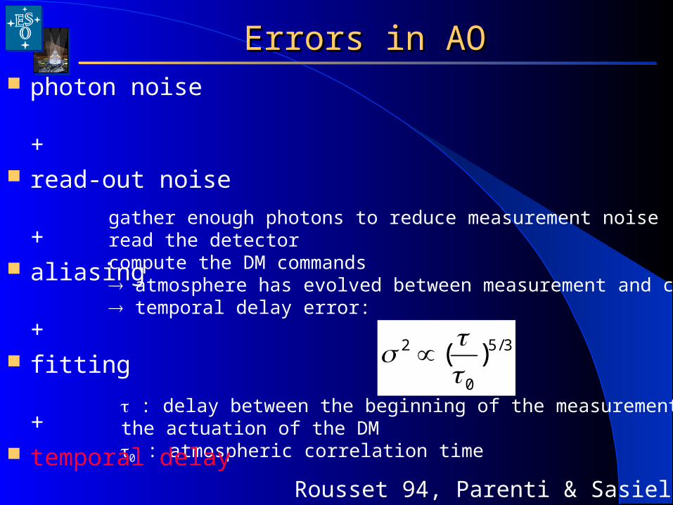
Errors in AOErrors in AO
gather enough photons to reduce measurement noiseread the detectorcompute the DM commands atmosphere has evolved between measurement and command temporal delay error:
3/5
0
2 )(
: delay between the beginning of the measurement and the actuation of the DM0 : atmospheric correlation time
Rousset 94, Parenti & Sasiela 94
photon noise
+ read-out noise
+ aliasing
+ fitting
+ temporal delay

Why closed loop ?Why closed loop ? There is a good reconstruction algo (=get the right
answer in 1 iteration). Hardware issues:
DM hysteresis (i.e. don’t know accurately what shape DM has)
WFS dynamic range: much reduced if need only to measure residuals.E.g. on SH, Open loop requires more pixels more noise
WFS linearity range : for some WFSs, this is critical: SH with quad-cell, Curvature WFS…
Closed loop hides calibration / non-linearity problems
Closed loop statistics harder to model PSF reconstruction gets harder Loop optimization harder

Interaction matrix in (MC)AOInteraction matrix in (MC)AO
Move one actuator on the deformable mirror response DM influence function
Propagate this DM shape to the conjugation height of the WFS (usually ground)
measure of the response current WFS ( b ) store b in the interaction matrix (M)
as many rows as measurements and columns as actuators
Invert that matrix (+ filter some modes) command matrix: M+ (LS estimate)
command vector c of the DM :
bMMMbMc tt
1)(

Optimizing control matrixOptimizing control matrix
Problem: previous method doesn’t know anything about: Atmospheric turbulence power spectrum
A priori knowledge MAP Minumum variance methods (e.g. Ellerbroek 1994) […]
Guide star magnitude Temporal evolution (turbulent speed, system
bandwidth) See talks by Marcos van Dam & J.M. Conan

A word on modal controlA word on modal control
The previously generated command matrix controls “mirror modes”
Some filtering is usually required (there are ill conditioned modes)
Strategy: filter out “unlikely” modes Project system control space on some orthogonal
polynomials, like: Zernike polynomials KL-polynomials […]
Use atmospheric knowledge to guess which of those modes are not likely to appear in the atmosphere (see talk by J.-M. Conan)

Optimized modal controlOptimized modal control
Must evaluate S/N of measurements and include it in command matrix
Gendron & Léna (1994, 1995) Ellerbroek et al., 1994 Idea: low order modes should have better S/N because they
have lower spatial frequencies E.g. Tip-tilt has a lot of signal (measured over a large pupil) High orders need more integration time to get enough signal.
Compute, for each corrected mode, the optimal bandwidth: allows in effect to change integration time
Need to estimate Noise variance (at first in open loop) PSD of mode fluctuations Sys transfer fn
Include these gains in the command matrix:
toptWUVGM

RequirementsRequirements
We need to: Identify delays in the system Model system’s transfer function Measure the measurement noise in the
WFS Atmospheric noise

Major AO delay sourcesMajor AO delay sources
Integration time: need to get photons CCD read-out time ~ integration time WFS measurement processing:
Flat-fielding Thresholding CCD de-scrambling
Matrix multiplication Actuation (time between sending
command and new DM shape) NOTE: some of these operation can be (and
are) pipelined to increase performance
~4ms
~1ms
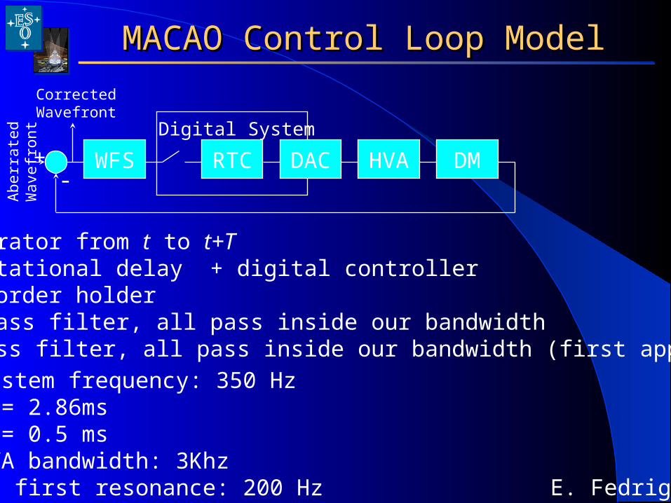
MACAO Control Loop ModelMACAO Control Loop Model
WFS DACRTC HVA DM+-
Digital System
WFS: integrator from t to t+TRTC: computational delay + digital controllerDAC: zero-order holderHVA: low-pass filter, all pass inside our bandwidthDM: low-pass filter, all pass inside our bandwidth (first approximation)
System frequency: 350 HzT = 2.86msτ = 0.5 msHVA bandwidth: 3KhzDM first resonance: 200 Hz
CorrectedWavefront
Abe
rrat
edW
avef
ront
E. Fedrigo

AO open loop transfer functionAO open loop transfer function
H(s): Open loop transfert function C(s): Compensator’s continuous transfer
function (usually ~integral…)
T: Integration time (= sampling period (+ read-out))
: Pure delay Simplistic model (continuous, not all errors…),
can of course be improved
)(]exp[]exp[1
)(2
sCsTs
TssH
s
KsC )(

Noise estimationNoise estimation
It is possible to compute (Gendron & Léna 1994):
dfgfHbdfbfBfTgfHgncor ),())()((),()( 000
Bandwidth error Noise errorResidual erroron a mode

Noise estimationNoise estimation
It is possible to compute (Gendron & Léna, 1994):
where :0(g): residual phase error on a mode (for a mode)g: modal gain for mode ( BW), Fe: sampling freqHcor(f,g): correction transfer functionT(f): PSD of fluctuations due to turbulenceB(f): PSD of noise propagated on modeb0: average level of B(f):
Hn: transfer fn white noise input noise output on mirror mode controls.
dfgfHbdfbfBfTgfHgncor ),())()((),()( 000
2/
0
)(2
0eF
e
dffBF
b

Measuring the noise varianceMeasuring the noise variance
Gendron &
Lena 1994

Optimized modal controlOptimized modal control
Correction BW not very sensitive to b0 estimate
Gendron &
Lena 1994

Optimized modal controlOptimized modal control
High order modes have less BW
than low order modes
Gendron &
Lena 1994

Closed loop optimizationClosed loop optimization Problems:
noise estimation+transfer function model need (too) good accuracy
Turbulence is evolving rapidly must adapt gains Non linearity problems in WFS possible (e.g. curvature)
Rigaut, 1993: Use closed-loop data as well (PUEO)
Dessenne et al 1998: Minimization of residuals of WFS error Reconstruction of open loop data from CL
measurements Algorithm must be quick to follow turbulence evolution (few
minutes) Iterative process: initial gain “guess” (from simulation) improved with
closed-loop data, by minimizing WFE estimate.
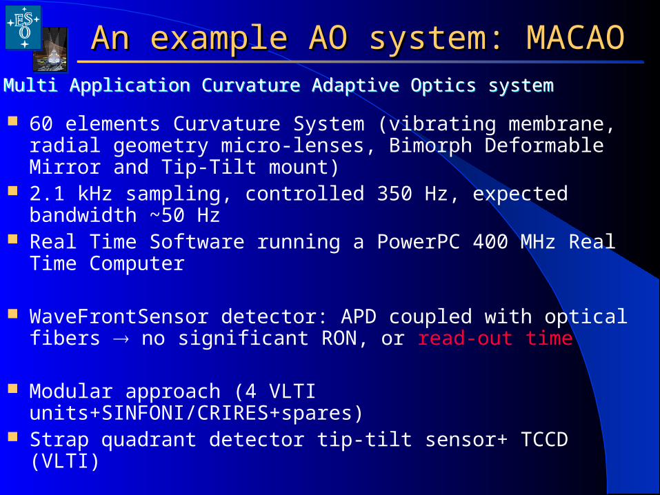
An example AO system: MACAOAn example AO system: MACAO
60 elements Curvature System (vibrating membrane, radial geometry micro-lenses, Bimorph Deformable Mirror and Tip-Tilt mount)
2.1 kHz sampling, controlled 350 Hz, expected bandwidth ~50 Hz
Real Time Software running a PowerPC 400 MHz Real Time Computer
WaveFrontSensor detector: APD coupled with optical fibers no significant RON, or read-out time
Modular approach (4 VLTI units+SINFONI/CRIRES+spares) Strap quadrant detector tip-tilt sensor+ TCCD (VLTI)
Multi Application Curvature Adaptive Optics systemMulti Application Curvature Adaptive Optics system

A real system: MACAOA real system: MACAO
ATM+TEL
GuideProbe
TelescopeControl
M2
TTM
DM
CWFS
AdaptiveControl
Low Pass
Low Pass
CorrectedWavefront
350Hz
5Hz
1Hz
1Hz
E. Fedrigo

LGS ControlLGS Control
ATM+TEL
GuideProbe
TelescopeControl
M2
TTM
DM
Trombone
LGSDefocus
CWFS
AdaptiveControl
Low Pass
Low Pass
Low Pass
CorrectedWavefront
Airmass
500Hz
5Hz
1Hz
0.03Hz
1Hz
E. Fedrigo

100
101
102
-50
-40
-30
-20
-10
0
10M A C A O 1 inner ring c los ed-loop e rror t rans fe r func t ion fo r g= 70% , tu rb= 10 ,25,50%
frequenc y (H z )
ga
in (
dB
)
1 00
101
102
-50
-40
-30
-20
-10
0
10M A C A O 1 inner ring c los ed-loop e rror t rans fe r func t ion fo r g= 70% , tu rb= 10 ,25,50%
frequenc y (H z )
ga
in (
dB
)
System BandwidthSystem Bandwidth
Plots: courtesy of Liviu Ivanescu, ESOPlots: courtesy of Liviu Ivanescu, ESO(0.45” seeing in V)
Measured Close-Loop Error Transfer FunctionMeasured Close-Loop Error Transfer Function
Predictive & more elaborate controlPredictive & more elaborate control
How to improve control BW ? Turbulence is predictable
Schwarz, Baum & Ribak, 1994 Aitken & McGaughey, 1996
Several approaches (at least): Madec et al., 1991, Smith compensator : takes lag into account Paschall & Anderson, 1993 : Kalman filtering : see talk by Don Gavel Wild, 1996 : cross covariance matrices Dessenne, Madec, Rousset 1997: predictive control law
There is a performance increase in BW limited system Layers are not separated, so “hard job” Unfortunately, gain seems small for current single GS AO systems.
Static aberrations need to be taken into account: residual mode error 0 Telescope vibrations need special attention

Predictive controlPredictive control
Dessenne, Madec, Rousset, 1999

MCAO / GLAOMCAO / GLAO
General case of AO, Several WFSs, several DMs
Observation / optimization direction
Measurement Direction 1
Measurement Direction 2
Challenge:find clever ways to work in closed loop !Are the sensors always seeing the correction ?

The futureThe future
MCAO Allow better temporal predictability if layers are separated Control of several DMs, WFSs, possibly in “open loop”
ELTs / ExAO: fast reconstructors, because MVM grows quickly w/ number of actuators FFT-based Sparse matrix […] predictive methods to the rescue !?
Segmentation Algorithms investigated to use AO WFS info to co-phase
segmented telescopes Kalman filtering
Optimize correction in closed loop, reliable noise estimates, complex systems
Applicable to MCAO


