Fundamentals of Hierarchical Linear and Multilevel Modeling · CHAPTER 1. FUnDAMEnTALs OF...

3

Fundamentals of Hierarchical Linear and Multilevel Modeling

G. David Garson

INTRODUCTION

Hierarchical linear models and multilevel models are variant terms for what are broadly called linear mixed models (LMM). These models handle data where observations are not independent, correctly modeling correlated error. Uncorrelated error is an important but often violated assumption of statistical procedures in the general linear model family, which includes analysis of variance, correlation, regression, and factor analysis. Violations occur when error terms are not independent but instead cluster by one or more grouping variables. For instance, predicted student test scores and errors in predicting them may cluster by classroom, school, and municipality. When clustering occurs due to a grouping factor (this is the rule, not the exception), then the standard errors computed for prediction parameters will be wrong (ex., wrong b coefficients in regression). Moreover, as is shown in the application in Chapter 6 in this volume, effects of predictor variables may be misinterpreted, not only in magnitude but even in direction.

Linear mixed modeling, including hierarchical linear modeling, can lead to substantially different conclusions compared to conventional regression analysis. Raudenbush and Bryk (2002), citing their 1988 research on the increase over time of math scores among students in Grades 1 through 3, wrote that with hierarchical linear modeling,

The results were startling—83% of the variance in growth rates was between schools. In contrast, only about 14% of the variance in initial status was between schools, which is consistent with results typically encountered in cross-sectional studies of school effects. This analysis identified substantial differences among schools that conventional models would not have detected because such analyses do not allow for the partitioning of learning-rate variance into within- and between-school components. (pp. 9–10)

1

4 PART I . GUIDE

Linear mixed models are a generalization of general linear models to better support analysis of a continuous dependent variable for the following:

1. Random effects: For when the set of values of a categorical predictor variable are seen not as the complete set but rather as a random sample of all values (ex., when the variable “product” has values representing only 30 of a possible 142 brands). Random effects modeling allows the researcher to make inferences over a wider population than is possible with regression or other general linear model (GLM) methods.

2. Hierarchical effects: For when predictor variables are measured at more than one level (ex., reading achievement scores at the student level and teacher–student ratios at the school level; or sentencing lengths at the offender level, gender of judges at the court level, and budgets of judicial districts at the district level). The researcher can assess the effects of higher levels on the intercepts and coefficients at the lowest level (ex., assess judge-level effects on predictions of sentencing length at the offender level).

3. Repeated measures: For when observations are correlated rather than independent (ex., before–after studies, time series data, matched-pairs designs). In repeated measures, the lowest level is the observation level (ex., student test scores on multiple occasions), grouped by observation unit (ex., students) such that each unit (student) has multiple data rows, one for each observation occasion.

The versatility of linear mixed modeling has led to a variety of terms for the models it makes possible. Different disciplines favor one or another label, and different research targets influence the selection of terminology as well. These terms, many of which are discussed later in this chapter, include random intercept modeling, random coefficients modeling, random coefficients regression, random effects modeling, hierarchical linear modeling, multilevel modeling, linear mixed modeling, growth modeling, and longitudinal modeling. Linear mixed models in some disciplines are called “random effects” or “mixed effects” models. In economics, the term “random coefficient regression models” is used. In sociology, “multilevel modeling” is common, alluding to the fact that regression intercepts and slopes at the individual level may be treated as random effects of a higher (ex., organizational) level. And in statistics, the term “covariance components models” is often used, alluding to the fact that in linear mixed models one may decompose the covariance into components attributable to within-groups versus between-groups effects. In spite of many different labels, the commonality is that all adjust observation-level predictions based on the clustering of measures at some higher level or by some grouping variable.

The “linear” in linear mixed modeling has a meaning similar to that in regres-sion: There is an assumption that the predictor terms on the right-hand side of the estimation equation are linearly related to the target term on the left-hand side. Of course, nonlinear terms such as power or log functions may be added to the predic-tor side (ex., time and time-squared in longitudinal studies). Also, the target variable may be transformed in a nonlinear way (ex., logit link functions). Linear mixed model (LMM) procedures that do the latter are “generalized” linear mixed models.

CHAPTER 1. FUnDAMEnTALs OF HIERARCHICAL LInEAR AnD MULTILEVEL MODELInG 5

Just as regression and GLM procedures can be extended to “generalized general linear models” (GZLM), multilevel and other LMM procedures can be extended to “generalized linear mixed models” (GLMM), discussed further below.

Linear mixed models for multilevel analysis address hierarchical data, such as when employee data are at level 1, agency data are at level 2, and department data are at level 3. Hierarchical data usually call for LMM implementation. While most multilevel modeling is univariate (one dependent variable), multivariate multilevel modeling for two or more dependent variables is available also. Likewise, models for cross-classified data exist for data that are not strictly hierarchical (ex., as when schools are a lower level and neighborhoods are a higher level, but schools may serve more than one neighborhood).

The researcher undertaking causal modeling using linear mixed modeling should be guided by multilevel theory. That is, hierarchical linear modeling pos-tulates that there are cross-level causal effects. Just as regression models postulate direct effects of independent variables at level 1 on the dependent variable at level 1, so too, multilevel models specify cross-level interaction effects between vari-ables located at different levels. In doing multilevel modeling, the researcher postulates the existence of mediating mechanisms that cause variables at one level to influence variables at another level (ex., school-level funding may posi-tively affect individual-level student performance by way of recruiting superior teachers, made possible by superior financial incentives).

Multilevel modeling tests multilevel theories statistically, simultaneously modeling variables at different levels without necessary recourse to aggrega-tion or disaggregation.1 Aggregation and disaggregation as used in regression models run the risk of ecological fallacy: What is true at one level need not be true at another level. For instance, aggregated state-level data on race and lit-eracy greatly overestimate the correlation of African American ethnicity with illiteracy because states with many African Americans tend to have higher illiteracy for all races. Individual-level data shows a low correlation of race and illiteracy.

WHY USE LINEAR MIXED/HIERARCHICAL LINEAR/ MULTILEVEL MODELING?

Why not just stick with tried-and-true regression models for analysis of data? The central reason, noted above, is that linear mixed models handle random effects, including the effects of grouping of observations under higher entities (ex., grouping of employees by agency, students by school, etc.). Clustering of observations within groups leads to correlated error terms, biased estimates of parameter (ex., regression coefficient) standard errors, and possible substantive mistakes when interpreting the importance of one or another predictor variable. Whenever data are sampled, the sampling unit as a grouping variable may well be a random effect. In a study of the federal bureaucracy, for instance, “agency”

6 PART I . GUIDE

might be the sampling unit and error terms may cluster by agency, violating ordinary least squares (OLs) assumptions.

Unlike OLs regression, linear mixed models take into account the fact that over many samples, different b coefficients for effects may be computed, one for each group. Conceptually, mixed models treat b coefficients as random effects drawn from a normal distribution of possible b’s, whereas OLs regression treats the b parameters as if they were fixed constants (albeit within a confidence inter-val). Treating “agency” as a random rather than fixed factor will alter and make more accurate the ensuing parameter estimates. Put another way, the misestima-tion of standard errors in OLs regression inflates Type 1 error (thinking there is relationship when there is not: false positives), whereas mixed models handle this potential problem. In addition, LMM can handle a random sampling vari-able like “agencies,” even when there are too many agencies to make into dummy variables in OLs regression and still expect reliable coefficients.

In summary, OLs regression and GLM assume error terms are independent and have equal error variances, whereas when data are nested or cross-classified by groups, individual-level observations from the same upper-level group will not be independent but rather will be more similar due to such factors as shared group history and group selection processes. While random effects associated with upper-level random factors do not affect lower-level population means, they do affect the covariance structure of the data. Indeed, adjusting for this is a central point of LMM models and is why linear mixed models are used instead of regres-sion and GLM, which assume independence.

It is true that analysis of variance and other GLM methods have been adapted to handle non-independent models also, but these adaptations are problematic. In estimating model parameters when there are random effects, it is necessary to adjust for the covariance structure of the data. The adjustment made by GLM assumes uncorrelated error (that is, it assumes data independence). Lack of data independence is present in multilevel data when the sampling unit (ex., cities, schools, agencies) displays intraclass correlation. LMM does not assume data independence. In addition to handling correlated error, LMM also has the advan-tage of using maximum likelihood (ML) and restricted maximum likelihood (REML) estimation. GLM produces optimum estimates only for balanced designs (where the groups formed by the factors are equal in size), whereas ML and REML yield asymptotically efficient estimators even for unbalanced designs. ML and REML estimates are normal for large samples (they display asymptotic normality), allowing significance testing of model covariance parameters, something difficult to do in GLM. In contrast, GLM estimates parameters as if they were fixed, calculating variance components based on expected mean squares.

Logistic regression also does not provide for random effects variables, nor (even in the multinomial version) does it support near-continuous dependents (ex., test scores) with a large number of values. Binning such variables into categories, as is sometimes done, loses information and attenuates correlation. However, logistic


multilevel models are possible using generalized linear mixed modeling proce-dures, available in sPss, sAs, and other statistical packages.

TYPES OF LINEAR MIXED MODELS

Linear mixed modeling supports a very wide variety of models, too extensive to enumerate here. As mentioned above, different disciplines and authors have employed differing labels for specific types of models, adding to the seeming complexity of the subject. In this section, the most common types of models are defined, using the most widely applied labels.

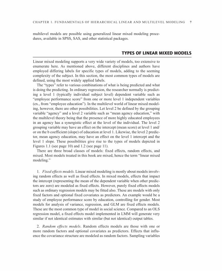
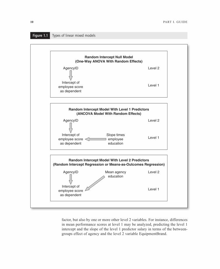
The “types” refer to various combinations of what is being predicted and what is doing the predicting. In ordinary regression, the researcher normally is predict-ing a level 1 (typically individual subject level) dependent variable such as “employee performance score” from one or more level 1 independent variables (ex., from “employee education”). In the multilevel world of linear mixed model-ing, however, there are other possibilities. Let level 2 be defined by the grouping variable “agency” and a level 2 variable such as “mean agency education,” with the multilevel theory being that the presence of more highly educated employees in an agency has a synergistic effect at the level of the individual. The level 2 grouping variable may have an effect on the intercept (mean score) at level 1 and/or on the b coefficient (slope) of education at level 1. Likewise, the level 2 predic-tor, mean agency education, may have an effect on the level 1 intercept and the level 1 slope. These possibilities give rise to the types of models depicted in Figures 1.1 (see page 10) and 1.2 (see page 11).

There are three broad classes of models: fixed effects, random effects, and mixed. Most models treated in this book are mixed, hence the term “linear mixed modeling.”

1. Fixed effects models. Linear mixed modeling is mostly about models involv-ing random effects as well as fixed effects. In mixed models, effects that impact the intercept (representing the mean of the dependent variable when other predic-tors are zero) are modeled as fixed effects. However, purely fixed effects models such as ordinary regression models may be fitted also. These are models with only fixed factors and optional fixed covariates as predictors. An example would be a study of employee performance score by education, controlling for gender. Most models for analysis of variance, regression, and GLM are fixed effects models. These are the most common type of model in social science. Compared to an OLs regression model, a fixed effects model implemented in LMM will generate very similar if not identical estimates with similar (but not identical) output tables.

2. Random effects models. Random effects models are those with one or more random factors and optional covariates as predictors. Effects that influ-ence the covariance structure are modeled as random factors. sampling variables

8 PART I . GUIDE

(ex., state, where individuals are sampled within a sample of states; subject, where a sample of subjects have repeated measures over time) are random fac-tors, as is any grouping variable where the clustering of effects creates correlated error. An example would be a study of employee performance score at level 1 by agency at level 2, controlling for salary level at level 1. score would be the dependent variable, agency the random factor (assuming only a random sample of agencies were studied), and salary the covariate. The level 1 intercept of score may be modeled as a random effect of agency at level 2. Likewise, the level 1 slope of employee education might be modeled as a random effect of agency. If only the intercept is modeled, it is a random intercept model.2 If the slope is modeled as well, it is a random coefficients model. some authors use the term “hierarchical linear model” to refer to random effects models in which both intercepts and slopes are modeled.

3. Mixed models. Mixed models, naturally, are ones with both fixed and ran-dom effects. A given effect may be both fixed and random if it contributes to both the intercept and the covariance structure for the model. Predictors at any level are typically included as fixed effects. For instance, covariates at level 2 are nor-mally included as fixed effect variables. slopes of variables at lower levels may be random effects of higher-level variables. Grouping variables (ex., school, agency) at any level are random factors.

Hierarchical linear models (HLM) are a type of mixed model with hierarchical data—that is, where nested data exist at more than one level (ex., student-level data and school-level data, with students nested within schools). In explaining a dependent variable, HLM models focus on differences between groups (ex., schools) in relation to differences within groups (ex., among students within schools). While it is possible to construct one-level models in linear mixed modeling, most use of LMM can be seen as one or another form of HLM, so the two terms are often used synonymously in spite of nuanced differences.

Random intercept models are models where only the intercept of the level 1 dependent variable is modeled as an effect of the level 2 grouping variable and possibly other level 1 or level 2 (or higher) covariates. Random coefficients mod-els are ones where the coefficient(s) of lower-level predictor(s) is/are modeled as well. There are several major types of random intercept and random coefficient models, enumerated below (see Table 1.1).

• The null model, also called the “unconditional model” or a “one-way AnOVA with random effects,” is a type of random intercept model that predicts the level 1 intercept of the dependent variable as a random effect of the level 2 grouping variable, with no other predictors at level 1 or 2 in a two-level model. For instance, differences in mean performance scores may be analyzed in terms of the random effect of agency at level 2. The researcher is testing to see if there is an agency effect. The null model is used to calculate the intraclass correlation coefficient (ICC), which is a test of the need for mixed modeling as discussed in


Chapter 2. The null model also serves as a “baseline model” for purposes of comparison with later, more complex models. note that a model is “conditional” by the presence of predictors at level 1 or level 2. since the researcher almost always employs predictor variables and is not simply interested in the null model, most mixed models are conditional. The central point of LMM often is to assess the difference between the researcher’s conditional model and the null model without predictors. The likelihood ratio test (discussed in Chapter 2) can be used to assess this difference.

• One-way ANCOVA with random effects models. It is also possible to have a level 1 covariate and still predict the level 1 intercept (but not the slope of the level 1 covariate) as a random effect of the level 2 grouping variable, with no other level 2 predictors. For instance, differences in mean performance scores (the intercepts) may be analyzed as predicted by salary at level 1, predicting only the level 1 inter-cept of performance scores in terms of the between-groups effect of agency as a grouping variable.

• Random intercept regression models are also called “means-as-outcomes regression models.” This variant of the random intercept model predicts the level 1 intercept on the basis of the level 2 grouping variable and also on the basis of one or more level 2 random effect predictors. For instance, differences in mean per-formance scores (the intercepts) may be analyzed, predicting the level 1 intercept in terms of the between-groups effect of agency and the level 2 random effect variable EquipmentBrand (a factor representing a sample of some of many brands of equipment, where different agencies used different brands).

• Random intercept ANCOVA models are also called “means-as-outcomes AnCOVA models.” This type is simply a random intercept regression model in which there is also a level 1 covariate treated as a fixed effect (slope not predicted by level 2). some authors would classify this as another type of random intercept regression model.

• Random coefficients (RC) models, also called “random coefficient regres-sion models” or “multilevel regression models,” are a type of mixed model with hierarchical data. The level 1 dependent is predicted by at least one level 1 covariate. The slope of this covariate and the intercept are predicted by the ran-dom effect of the grouping variable at level 2. That is, each group at the higher level (ex., agency level) is assumed to have a different regression slope as well as a different intercept for purposes of predicting a level 1 dependent variable. While this could be visualized by using OLs regression by superimposing the n regression lines for the n schools, LMM incorporates this variability of regres-sion lines into a single analysis.

• Full random coefficients models, also called “intercepts-and-slopes-as-outcomes models,” are a type of RC model in which the level 1 slopes and intercepts are modeled not only by the level 2 grouping variable as a random

10 PART I . GUIDE

factor, but also by one or more other level 2 variables. For instance, differences in mean performance scores at level 1 may be analyzed, predicting the level 1 intercept and the slope of the level 1 predictor salary in terms of the between-groups effect of agency and the level 2 variable EquipmentBrand.

Random Intercept Null Model(One-Way ANOVA With Random Effects)

AgencyID

Intercept ofemployee scoreas dependent

Level 2

Level 1

Random Intercept Model With Level 1 Predictors(ANCOVA Model With Random Effects)

AgencyID


Slope timesemployeeeducation

Level 2

Level 1

Random Intercept Model With Level 2 Predictors(Random Intercept Regression or Means-as-Outcomes Regression)

AgencyID


Mean agencyeducation

Level 2

Level 1

Figure 1.1 Types of linear mixed models


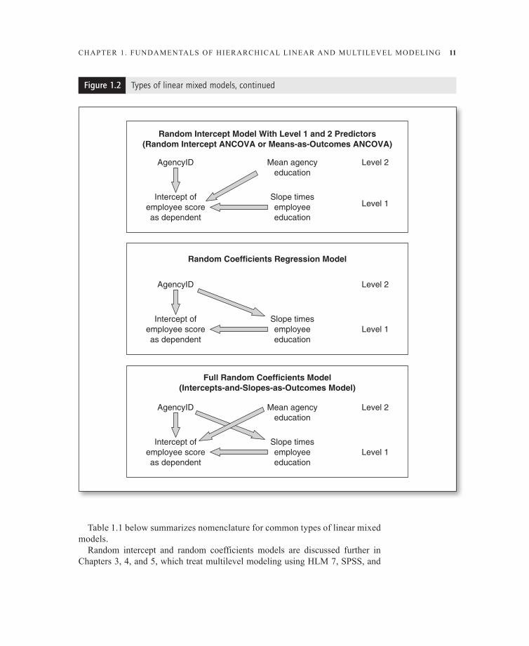
Table 1.1 below summarizes nomenclature for common types of linear mixed models.

Random intercept and random coefficients models are discussed further in Chapters 3, 4, and 5, which treat multilevel modeling using HLM 7, sPss, and

Random Intercept Model With Level 1 and 2 Predictors(Random Intercept ANCOVA or Means-as-Outcomes ANCOVA)

AgencyID





Level 2

Level 1

Level 2

Level 1

Random Coefficients Regression Model

AgencyID



Level 2

Level 1

Full Random Coefficients Model(Intercepts-and-Slopes-as-Outcomes Model)

AgencyID



Figure 1.2 Types of linear mixed models, continued

12 PART I . GUIDE

sAs software, respectively. In Chapter 6, Forrest C. Lane, Kim F. nimon, and J. Kyle Roberts further develop the topic in their article, “A Random Intercepts Model of Part-Time Employment and standardized Testing Using sPss.” In Chapter 7, Carissa L. shafto and Jill L. Adelson present “A Random Intercept Regression Model Using HLM: Cohort Analysis of a Mathematics Curriculum for Mathematically Promising students.” Then, in Chapter 8, Gregory J. Palardy presents “Random Coefficients Modeling With HLM: Assessment Practices and the Achievement Gap.” Finally, in Chapter 9, shevaun neupert presents “Emotional Reactivity to Daily stressors Using a Random Coefficients Model With sAs PROC MIXED: A Repeated Measures Analysis.”

GENERALIZED LINEAR MIXED MODELS

Generalized linear mixed models serve similar purposes to the models already discussed except that the “generalized” label means that new algorithms have been added to support a variety of link functions. Link functions, of course, are transforms of the dependent variable similar to that found, for instance, in binary

Table 1.1 Six Common Types of Two-Level Linear Mixed Models

I. Only the intercept is modeled as a random effect.

A. no level 1 covariates1. The null model, also called the unconditional model or one-way AnOVA with random effects

B. Level 1 covariates only2. Random intercept model: AnCOVA with random effects

C. Level 2 covariates only3. Random intercept regression: “means as outcomes regression”

D. Both level 1 and level 2 covariates4. Random intercept AnCOVA: “means as outcomes AnCOVA”

II. One or more level 1 slopes as well as the intercept are modeled.

A. no level 1 covariatesnot applicable: A level 1 covariate must exist to have a slope to model!

B. Level 1 covariates only1. Random coefficients regression

C. Level 2 covariates onlynot applicable

D. Both level 1 and level 2 covariates2. Full random coefficients model: “intercepts and slopes as outcomes”


logistic regression, where what is predicted is not the dependent variable itself (using the identity link function of OLs regression) but instead is the logit (the natural log of the odds that the dependent equals 1) of the dependent variable. Although the predictor side of the equation must be linearly related to the link function of the dependent, the original values of the predictor variables may be nonlinearly related to the original values of the dependent variable. A large number of link functions are possible, only some of which are currently supported by statistical packages for hierarchical linear modeling. Of fundamental importance is that generalized linear mixed modeling supports dependent variables that are not continuous and not normally distributed, as is required by ordinary regression and other general linear model procedures.

Although GLMM is not the focus of this book, it is important that the researcher be aware of the possibilities supported by generalized linear mixed modeling and be assured that the data at hand are best modeled by the LMM models described in this volume rather than by GLMM methods. nonetheless, even if GLMM is selected due to the nature of the researcher’s dependent variable, nearly all of the LMM considerations discussed in the present volume still apply.

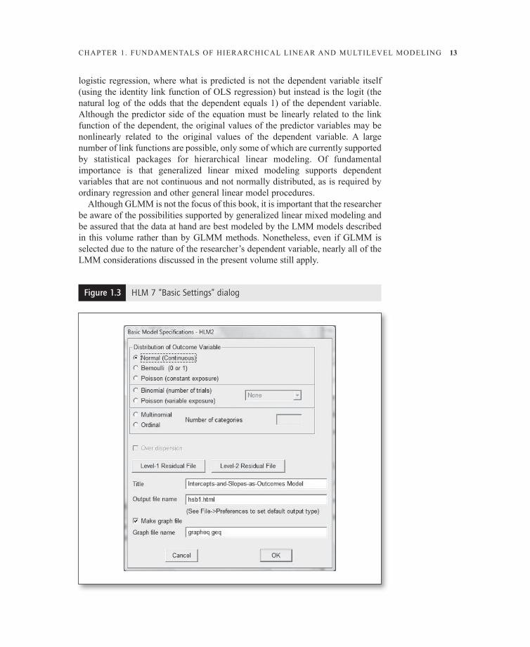
Figure 1.3 HLM 7 “Basic Settings” dialog

14 PART I . GUIDE

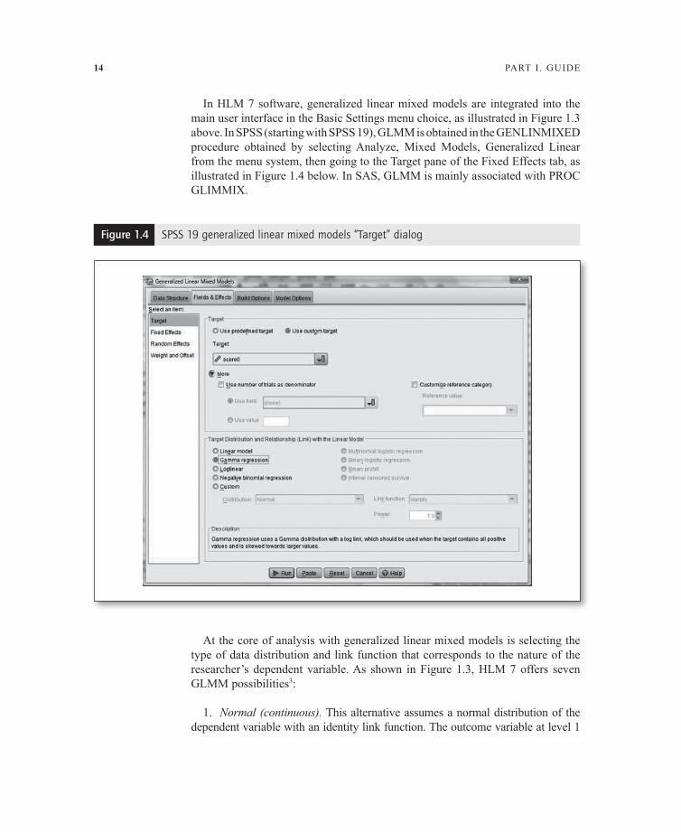
In HLM 7 software, generalized linear mixed models are integrated into the main user interface in the Basic settings menu choice, as illustrated in Figure 1.3 above. In sPss (starting with sPss 19), GLMM is obtained in the GEnLInMIXED procedure obtained by selecting Analyze, Mixed Models, Generalized Linear from the menu system, then going to the Target pane of the Fixed Effects tab, as illustrated in Figure 1.4 below. In sAs, GLMM is mainly associated with PROC GLIMMIX.

Figure 1.4 SPSS 19 generalized linear mixed models “Target” dialog

At the core of analysis with generalized linear mixed models is selecting the type of data distribution and link function that corresponds to the nature of the researcher’s dependent variable. As shown in Figure 1.3, HLM 7 offers seven GLMM possibilities3:

1. Normal (continuous). This alternative assumes a normal distribution of the dependent variable with an identity link function. The outcome variable at level 1


may have any value on a continuous scale (ex., employee-level performance scores). This option creates the same models as for ordinary linear mixed modeling.

2. Bernoulli. This alternative assumes a Bernouilli distribution, which is a special case of the binomial distribution, employing a logit link function. In a Bernouilli model, the outcome variable at level 1 (ex., employee-level retirement status) has only two outcomes (ex., not retired = 0, retired = 1).

3. Binomial (number of trials). This alternative assumes a dependent variable with a binomial distribution and a logit link function, corresponding to binary logistic regression.

4. Poisson (constant exposure). This alternative assumes a dependent variable reflecting count data (hence non-negative integer values) with a log link function. The “constant exposure” term, also called “equal exposure,” means each level 1 subject had the same chance to accumulate the count (ex., the same time interval).

5. Poisson (variable exposure). An example of this type would be a count of people displaying some trait in multiple cities of differing populations. The “exposure” varies since, all other things equal, larger cities might be expected to have a larger count. Like Poisson-constant exposure models, this alternative also assumes Poisson distribution of count data with a log link function, but the Poisson variance is weighted by the exposure variable.

6. Multinomial. This alternative assumes a multinomial distribution of the dependent variable, with a generalized logit link function. Multinomial data are categorical, such as “career choice” with values 1 = administrative, 2 = clerical, 3 = other. The coding values are arbitrary. A multinomial model is an extension of the Bernouilli model for dependents with more than two categories.

7. Ordinal. This alternative also assumes the dependent variable has a cate-gorical distribution, but the categories are ordered—for example, ordered from “strongly agree” to “strongly disagree.” The link function is cumulative logit.

sPss 19 offers eight link alternatives plus a “Custom” alternative. In addition, there is a checkbox for “Use number of trials as denominator,” which can convert the dependent variable into a ratio (ex., number of successes divided by number of trials, transforming a count into a rate). For categorical dependent variables, the sPss “TARGET” pane also allows the researcher to set the reference category to something other than the default, which is the highest-coded category.

1. Linear model. Used with an identity link function when the dependent is continuous and normal. This is the same as the “normal” selection in HLM 7.

2. Gamma regression. Used for dependents whose values are skewed toward larger values, this alternative assumes a gamma distribution with a log link.

16 PART I . GUIDE

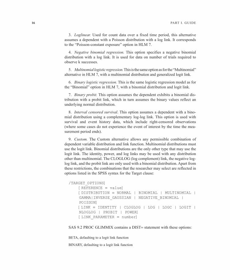
3. Loglinear. Used for count data over a fixed time period, this alternative assumes a dependent with a Poisson distribution with a log link. It corresponds to the “Poisson-constant exposure” option in HLM 7.

4. Negative binomial regression. This option specifies a negative binomial distribution with a log link. It is used for data on number of trials required to observe k successes.

5. Multinomial logistic regression. This is the same option as for the “Multinomial” alternative in HLM 7, with a multinomial distribution and generalized logit link.

6. Binary logistic regression. This is the same logistic regression model as for the “Binomial” option in HLM 7, with a binomial distribution and logit link.

7. Binary probit. This option assumes the dependent exhibits a binomial dis-tribution with a probit link, which in turn assumes the binary values reflect an underlying normal distribution.

8. Interval censored survival. This option assumes a dependent with a bino-mial distribution using a complementary log-log link. This option is used with survival and event history data, which include right-censored observations (where some cases do not experience the event of interest by the time the mea-surement period ends).

9. Custom. The Custom alternative allows any permissible combination of dependent variable distribution and link function. Multinomial distributions must use the logit link. Binomial distributions are the only other type that may use the logit link. The identity, power, and log links may be used with any distribution other than multinomial. The CLOGLOG (log complement) link, the negative log-log link, and the probit link are only used with a binomial distribution. Apart from these restrictions, the combinations that the researcher may select are reflected in options listed in the sPss syntax for the Target clause:

/TARGET_OPTIONS] [REFERENCE = value] [DISTRIBUTION = NORMAL | BINOMIAL | MULTINOMIAL | GAMMA|INVERSE_GAUSSIAN | NEGATIVE_BINOMIAL | POISSON] [LINK = IDENTITY | CLOGLOG | LOG | LOGC | LOGIT | NLOGLOG | PROBIT | POWER] [LINK_PARAMETER = number]

sAs 9.2 PROC GLIMMIX contains a DIsT= statement with these options:

BETA, defaulting to a logit link function

BInARY, defaulting to a logit link function


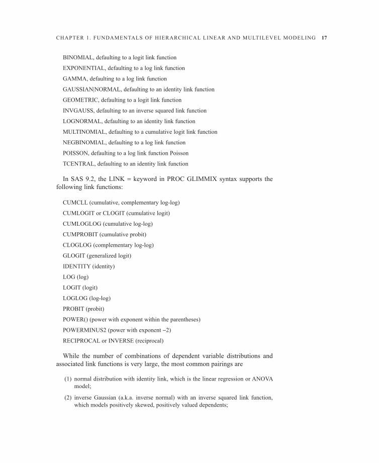
BInOMIAL, defaulting to a logit link function

EXPOnEnTIAL, defaulting to a log link function

GAMMA, defaulting to a log link function

GAUssIAn|nORMAL, defaulting to an identity link function

GEOMETRIC, defaulting to a logit link function

InVGAUss, defaulting to an inverse squared link function

LOGnORMAL, defaulting to an identity link function

MULTInOMIAL, defaulting to a cumulative logit link function

nEGBInOMIAL, defaulting to a log link function

POIssOn, defaulting to a log link function Poisson

TCEnTRAL, defaulting to an identity link function

In sAs 9.2, the LInK = keyword in PROC GLIMMIX syntax supports the following link functions:

CUMCLL (cumulative, complementary log-log)

CUMLOGIT or CLOGIT (cumulative logit)

CUMLOGLOG (cumulative log-log)

CUMPROBIT (cumulative probit)

CLOGLOG (complementary log-log)

GLOGIT (generalized logit)

IDEnTITY (identity)

LOG (log)

LOGIT (logit)

LOGLOG (log-log)

PROBIT (probit)

POWER() (power with exponent within the parentheses)

POWERMInUs2 (power with exponent -2)

RECIPROCAL or InVERsE (reciprocal)

While the number of combinations of dependent variable distributions and associated link functions is very large, the most common pairings are

(1) normal distribution with identity link, which is the linear regression or AnOVA model;

(2) inverse Gaussian (a.k.a. inverse normal) with an inverse squared link function, which models positively skewed, positively valued dependents;

18 PART I . GUIDE

(3) gamma distribution with a log link, also used for skewed dependents in gamma regression;

(4) multinomial distribution with a generalized or cumulative logit link, used for categorical or ordinal dependents in multinomial or ordinal regression;

(5) binomial distribution with a logit link, for binary logistic regression models;

(6) Poisson distribution with a log link, for count of events per fixed number of time periods in Poisson regression; and

(7) negative binomial distribution, used instead of Poisson for count data with overdispersion (when the variance is greater than the mean).

REPEATED MEASURES, LONGITUDINAL AND GROWTH MODELS

Increasingly, linear mixed modeling is the preferred approach when analyzing longitudinal data.4 studies in this category carry a variety of labels, including repeated measures designs, longitudinal analysis, and growth models. The common thread is the need to address the autocorrelation problem: Repeated observations for the same unit (ex., same employee with repeated performance score measures) exhibit clustering. Just as linear mixed models address the problem of clustering of measures and correlation of error by grouping or level variable, LMM addresses the problem of clustering by observation unit. Put another way, longitudinal data in LMM may be modeled by treating the multiple measures (ex., performance scores) as level 1 and the observation units (ex., employees) as level 2. Of course, level 2 units may still be nested within or cross-classified by levels 3 and 4 (ex., agency and department).

Repeated Measures

The object of repeated measures designs is to model within-subject variance. What is “within” a subject is, of course, the series of measurements taken over time for a given unit of analysis (typically an individual subject). Each subject will have multiple rows of data corresponding to multiple observation times. In terms of multilevel analysis, level 1 is within-subjects (for the variance among repeated measures for given individuals, on the average) and level 2 is between-subjects, with the observation unit (usually the individual) being a grouping vari-able for the measures. The grouping (subjects) variable can be used to assess the between-subjects random effect on a level 1 variable, such as employee perfor-mance test score. In a random intercepts model where there are level 1 covariates (predictors), this is done by creating one regression for each subject, generating multiple intercepts, where the true intercept is estimated as a random function of the intercepts of all the regressions. Random slopes may be generated in the same way to obtain a random coefficients model.


Longitudinal and Growth Models

Growth models are a common type of repeated measures linear mixed model in which time is modeled as a fixed and as a random effect on some measurement about the individual (ex., employee performance score). Visualized graphically, a “growth curve” for each employee can be charted in which time is the X-axis and the dependent variable, such as performance score, forms the Y-axis. Growth curves will vary by individual, depending on time-invariant and time-variant variables such as IQ or training workshop hours, respectively.

The object of growth modeling is not merely to see if there is a trend in score over time, but also to discover if the grouping variable has an effect on the trend (ex., if there is an employee effect) and if there is a pattern to the change in inter-cepts or coefficients over time. Assuming the time variable is measured in equal metric intervals, the time variable is a covariate and the growth pattern may be analyzed to see, for instance, if on average it increases linearly in steps, grows quadratically, or grows according to some other function of time.

Many different types of linear mixed models can be constructed in which time is a variable. To take one example, that of predicting a metric time series of employee performance scores at level 1 grouped by employee at level 2, the purpose of longitudinal analysis may be to see if and how the linear correlation of score and time is influenced by employee-specific effects. Time may be modeled as a fixed effect to capture the linear correlation, and in the fixed effects output, the b coefficient for time indicates how much, on average, each employee increases or decreases in score per measurement period. Time can also be modeled as a random effect to capture the effect of time nested within employees on the coefficient of time at level 1. (A regression is fitted for each employee, and a standard error is computed for the b coefficient of time in these regressions.)

If an unstructured covariance structure (see Chapter 2) is assumed, one will get covariance parameters for the intercept, for the b coefficient of the level 1 predictor, and for the covariance of the two. The larger the parameter for the intercept, the greater the variance of score among employees when time = 0, which is the start time. The larger the parameter for time as a random effect nested within employees, the greater (and more likely to be significant) the between-employees variability of the time coefficient. If there are level 2 (employee-level) covariates, these are treated as additional fixed factors. For instance, if education is such a covariate, fixed factors include time, education, and time*education. Time is also a random effect. The covariance parameter for the residual reflects the within-subjects variance, which is the variance of test scores across time for any given employee after controlling for other variables in the model (time, education, and the time*education interaction), and as such is the unexplained variance in the model.

There are many types of random coefficients growth models, some of which are illustrated in Chapters 3, 4, and 5. These provide an introductory guide to multilevel modeling using HLM 7, sPss, and sAs software, respectively.

20 PART I . GUIDE

Chapter 10, by David F. Greenberg and Julie A. Phillips, treats “Hierarchical Linear Modeling of Growth Curve Trajectories Using HLM,” dealing with a standard form of growth modeling. Chapter 11, by Jaime Lynn Maerten-Rivera, presents “A Piecewise Growth Model Using HLM7 to Examine Change in Teaching Practices Following a science Teacher Professional Development Intervention,” where piecewise growth models are ones where growth trajectories are divided and modeled separately. And in Chapter 12, Maike Luhmann and Michel Eid treat “studying Reaction to Repeated Life Events With Discontinuous Change Models Using HLM,” where discontinuous change models handle data where the individual growth trajectory is divided into discrete segments punctu-ated by discontinuities such as life events.

MULTIVARIATE MODELS

Multivariate linear mixed modeling (MLMM) is to LMM what multiple analysis of variance (MAnOVA) and covariance (MAnCOVA) are to general linear models (GLM): Each enables simultaneous analysis of multiple dependent variables defined at level 1 in a multilevel model. MLMM also goes under the label “hierarchical multivariate linear modeling” (HMLM).

In addition, nonlinear link functions can be added using multivariate general-ized linear mixed modeling (MGLMM), extending what is possible with general-ized linear mixed modeling (GLMM) of dependent variables considered singly.

MLMM and MGLMM are often used in analysis of latent variables, where the multiple level 1 dependents are seen as indicators for an underlying latent con-struct. This is the “multilevel latent outcome model.” For instance, measures of six specific skills, skill1 through skill6, may be seen as indicators for the latent variable “performance.” As another example, sammel, Lin, and Ryan (1999), in a study of several teratogenic (birth defect–inducing) agents, used MLMM to model the latent variable “teratogenic exposure” based on multiple indicators associated with the different agents.5

In a second application, MLMM and MGLMM may be used for joint analysis of what would otherwise be separate repeated measures analyses of different outcome variables. This is the “multilevel model for correlated outcomes” or “repeated measures multivariate linear mixed model” (see Molenberghs, 2007). In a third usage, MLMM and MGLMM may be used where skill1 through skill6 measure the same skill, but at different times; output1 through output6 measure objective productivity at different times; and the research focus is on testing a “parallel growth model.” MLMM can also be employed as a form of cluster analysis, based on longitudinal data on individuals’ behavior over time, classify-ing individuals according to differences in growth curves (Villarroel, 2009). A fifth type of usage of MLMM and MGLMM centers on analysis where the mul-tiple dependents are members of an exponential family, such as score, score-squared, and other exponential functions (see Gueorguieva, 2001). Multivariate


modeling is discussed further in Chapter 15, by Larry J. Brant and shan L. sheng, in their article, “Predicting Future Events From Longitudinal Data With Multivariate Hierarchical Models and Bayes’ Theorem Using sAs.” For more on MLMM in HLM 7, see Raudenbush, Bryk, Cheong, Congdon, and Du Toit (2011). For more on MLMM in sPss, see Heck, Thomas, and Tabata (2010, Ch. 7). For more on MLMM in sAs, see Wright (1998).

CROSS-CLASSIFIED MODELS

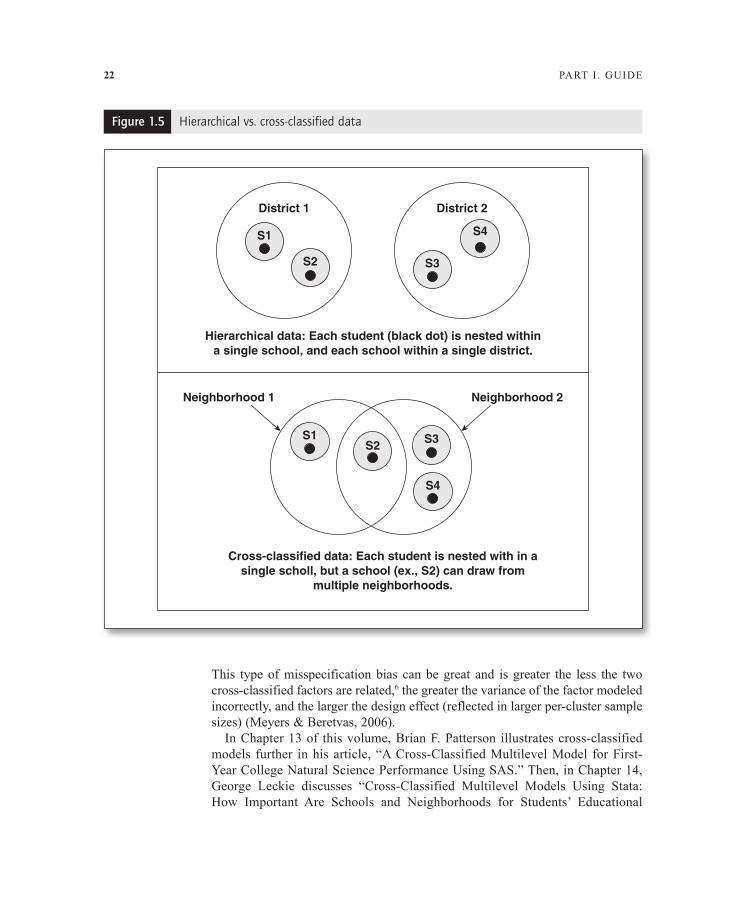
Cross-classified models handle data that do not meet the nesting assumptions of hierarchical models. Above, an example of assumed test scores are grouped by individual employee, with employees nested within agencies and agencies within departments. However, what if the data include employees who are employed by multiple agencies? In educational research, what if students are members of multiple classrooms rather than each student belonging to just one classroom? As another example, in repeated measures studies involving interviews of subjects, the same subject may be interviewed by more than one interviewer, and therefore the subject is cross-classified on the interviewer effect. such data, illustrated in Figure 1.5 below, are cross-classified and require cross-classified random effects modeling (see Beretvas, Meyers, & Rodriguez, 2005). Exclusively hierarchical data are less common than cross-classified data, and thus cross-classified linear mixed modeling (CCLMM; also called cross-classified multilevel measurement modeling [CCMMM], and cross-classified random effects modeling [CCREM]) is an important tool within the LMM family.

Applying hierarchical linear mixed modeling to cross-classified data can seri-ously bias variance component estimates as well as bias the estimation of the standard errors of the regression coefficients. Meyers and Beretvas (2006) found that such misspecification did not significantly affect parameter estimates for fixed effects, but did bias estimates for standard errors, and also biased estimates of variance components of the random effects, inflating Type 1 error. Luo and Kwok (2009), using simulation studies, likewise found that “ignoring a crossed factor causes overestimation of the variance components of adjacent levels and underestimation of the variance component of the remaining crossed factor” (p. 182). In the present volume, George Leckie (Chapter 14) similarly notes that ignoring cross-classification effects leads to overestimation of level 1 (ex., stu-dent) and level 2 (ex., school) effects using conventional hierarchical linear modeling. Moreover,

ignoring a crossed factor at the kth level causes underestimation of the standard error of the regression coefficient of the predictor associated with the ignored factor and overestimation of the standard error of the regression coefficient of the predictor at the (k-1)th level. (Luo & Kwok, 2009, p. 182)

22 PART I . GUIDE

This type of misspecification bias can be great and is greater the less the two cross-classified factors are related,6 the greater the variance of the factor modeled incorrectly, and the larger the design effect (reflected in larger per-cluster sample sizes) (Meyers & Beretvas, 2006).

In Chapter 13 of this volume, Brian F. Patterson illustrates cross-classified models further in his article, “A Cross-Classified Multilevel Model for First-Year College natural science Performance Using sAs.” Then, in Chapter 14, George Leckie discusses “Cross-Classified Multilevel Models Using stata: How Important Are schools and neighborhoods for students’ Educational

Hierarchical data: Each student (black dot) is nested withina single school, and each school within a single district.

District 1 District 2

S1

S2 S3

S4

Cross-classified data: Each student is nested with in asingle scholl, but a school (ex., S2) can draw from

multiple neighborhoods.

Neighborhood 1 Neighborhood 2

S1S2 S3

S4

Figure 1.5 Hierarchical vs. cross-classified data


Attainment?” For more on cross-classified models in HLM 7, see Raudenbush et al. (2011). For more on cross-classified models in sPss, see Heck, Thomas, and Tabata (2010, Ch. 8). For more on cross-classified models in sAs, see Beretvas (2008). All three packages support two- and three-level CCLMM models.

SUMMARY

Multilevel and hierarchical modeling through various types of linear mixed models has rapidly become a required asset in the statistical toolkit of researchers worldwide. By correctly modeling correlated error, which arises from the clustering of data at the group level, LMM models address a major shortcoming of regression, AnOVA, and other general linear model analyses. Failure to take correlated error into account can easily affect the researcher’s substantive conclusions. Whether used to model random effects, hierarchical effects, or repeated measures effects, linear mixed modeling is a versatile tool, applicable to a broad range of common research problems. Generalized linear mixed modeling incorporates nonlinear link functions of the dependent variable. Multivariate linear mixed modeling incorporates analysis of multiple dependent variables. Cross-classified linear mixed modeling handles crossed factors that depart from strictly hierarchical structure. All variants handle cross-level interaction terms as well as cross-level main effects, and all variants test multi-level theories without necessity to aggregate or disaggregate data — a commonly flawed practice in ordinary regression modeling. With this versatility and power, it is small wonder that courses on hierarchical linear modeling, multilevel modeling, and linear mixed modeling now pervade doctoral research programs.

After evaluating the research design and after screening data to meet the assumptions of LMM (to be discussed in Chapter 2), the researcher must select the type of model to explore. This depends on the research question. If the research interest is confined to understanding why mean values of the dependent variable vary, then a random intercept model may suffice. If, however, the research interest is in exploring the relative effects of predictor variables, a ran-dom coefficients model is ordinarily selected. If there are multiple dependent variables to be treated as a set, multivariate models are required. If data are not nested in a strictly hierarchical manner, cross-classified models will be needed. Models also vary by number of levels of data involved, though in practice nearly all linear mixed modeling is confined to analysis of two to four levels.

Within these broad categories, there are many variations on type of model. The null model models the dependent variable without predictors apart from the grouping variable(s). One-way random effects AnCOVA models predict the level 1 dependent as a fixed effect of level 1 covariates and a random effect of higher-level grouping variables. Random intercept regression models (means-as-outcomes regression models) add higher-level random effect predictors.

24 PART I . GUIDE

Random intercept AnCOVA models (means-as-outcomes AnCOVA) are a type of random intercept regression in which there are also level 1 fixed effect predic-tors. Random coefficients (RC) models predict level 1 slopes as well as inter-cepts. Full random coefficients models (intercepts-and-slopes-as-outcomes models) model level 1 slopes and intercepts as functions of higher-level group-ing factors and higher-level covariates. With any model, data for repeated mea-surements may be present, in which case some type of longitudinal or growth model may be undertaken.

In summary, linear mixed modeling is a versatile procedure that supports an extremely large number of variations of type of model, only some of which are mentioned in this chapter. Generalized linear mixed modeling (GLMM) sup-ports still more types, covering nonlinear link functions for a variety of data distributions of the dependent variable. In this way, GLMM supports linear mixed modeling for binary, ordinal, and multinomial logistic models; probit, gamma, and negative binomial regression models; Poisson regression models and models for interval-censored survival data such as used in event history analysis, to name a few.

Looking ahead, Chapter 2 presents considerations preliminary to multilevel analysis, focusing on meeting the assumptions of linear mixed modeling and on understanding how models are evaluated. Then, in the following three chapters, the details of implementing a number of types of basic linear mixed models are presented. Chapters 3 through 5 present the same models as implemented in HLM 7, sPss 19, and sAs 9.2, respectively. The remaining 10 chapters of this volume, written by authors from diverse fields, present further applications based on these statistical packages (plus one application illustrated for stata), all fol-lowing a standard format emphasizing how to implement and report data analysis for linear mixed models.

NOTES

1. It should be noted, though, that in practice some variables may represent aggregated scores.

2. some authors use the term “hierarchical linear model” to refer to random effects models in which both intercepts and slopes are modeled.

3. Different options are offered in HLM 7 for multivariate generalized linear mixed models.

4. For a discussion comparing repeated measures AnOVA and event history approaches, see schulz and Maas (2010).

5. This article also contains a useful comparison of GLMM methods with factor analysis and structural equation modeling as alternative approaches to modeling latent variables.

6. This may seem anomalous, but if factors are correlated, then modeling one of them in a hierarchical design will reduce some of the bias that otherwise would occur.


REFERENCES

Beretvas, s. n. (2008). Cross-classified random effects models. In A. A. O’Connell & D. B. McCoach (Eds.), Multilevel modeling of educational data (pp. 161–197). Charlotte, nC: Information Age Publishing.

Beretvas, s. n., Meyers, J. L., & Rodriguez, R. A. (2005). The cross-classified multilevel measurement model: An explanation and demonstration. Journal of Applied Measurement, 6(3), 322–341.

Gueorguieva, R (2001). A multivariate generalized linear mixed model for joint modelling of clustered outcomes in the exponential family. Statistical modeling, 1(3), 177–193.

Heck, R. H., Thomas, s. L., & Tabata, L. n. (2010). Multilevel and longitudinal modeling with IBM SPSS. new York: Routledge.

Luo, W., & Kwok, O. M. (2009). The impacts of ignoring a crossed factor in analyzing cross-classified data. Multivariate Behavioral Research, 44(2), 182–212.

Meyers, J. L., & Beretvas, s. n. (2006). The impact of inappropriate modeling of cross-classified data structures. Multivariate Behavioral Research, 41(4), 473–497.

Molenberghs, G. (2007). Random-effects models for multivariate repeated measures. Statistical Methods in Medical Research, 16(5), 387–397.

Raudenbush, s. W., & Bryk, A. s. (2002). Hierarchical linear models: Applications and data analysis methods (2nd ed.) (Advanced Quantitative Techniques in the social sciences series, no. 1). Thousand Oaks, CA: sage.

Raudenbush, s. W., Bryk, A. s., Cheong, Y. F., Congdon, R., & Du Toit, M. (2011). HLM 7: Hierarchical linear and nonlinear modeling. Lincolnwood, IL: scientific software International.

sammel, M., Lin, X., & Ryan, L. (1999). Multivariate linear mixed models for multiple outcomes. Statistics in Medicine, 18(17–18), 2479–2492.

schulz, W., & Maas, I. (2010). studying historical occupational careers with multilevel growth models. Demographic Research, 23(24), 669–696. Retrieved March 13, 2011, from http://www.demographic-research.org/volumes/vol23/24/23-24.pdf

Villarroel, L. (2009). Cluster analysis using multivariate mixed effects models. Statistics in Medicine, 28(20), 2552–2565.

Wright, s. P. (1998). Multivariate analysis using the MIXED procedure. Paper presented at the Twenty-Third Annual Meeting of sAs Users’ Group International, nashville, Tn (Paper 229). Retrieved March 14, 2011, from http://www2.sas.com/proceedings/sugi23/stats/p229.pdf

Date post:	19-May-2018
Category:	Documents
Upload:	duongbao
View:	237 times
Download:	4 times

Fundamentals of Hierarchical Linear and Multilevel Modeling · CHAPTER 1. FUnDAMEnTALs OF...

Documents