+ All Categories
Home > Documents > Fundamentals of mudrock chemostratigraphy: … Slide Booklet.pdfFundamentals of mudrock...

Fundamentals of mudrock chemostratigraphy: … Slide Booklet.pdfFundamentals of mudrock...

Date post: 17-Apr-2018
Category:
Upload: truongnhi
View: 229 times
Download: 2 times
Share this document with a friend
48
Fundamentals of mudrock chemostratigraphy: Handheld XRF analysis, calibration, and interpretation Harry Rowe Bruce Kaiser Bureau of Economic Geology Chief Scientist Jackson School of Geosciences Bruker Elemental The University of Texas at Austin Austin, TX GCAGS Short Course Austin, Texas October 20, 2012 INSTRUCTORS
Transcript

Fundamentals of mudrock chemostratigraphy:Handheld XRF analysis, calibration, and interpretation

Harry Rowe Bruce Kaiser Bureau of Economic Geology Chief Scientist Jackson School of Geosciences Bruker Elemental The University of Texas at Austin Austin, TX

GCAGS Short Course

Austin, TexasOctober 20, 2012

INSTRUCTORS

XRF Workshop

Dr Bruce Kaiser

1�

Instrument – The Basics � X-ray Tube Ag,

Rh or Re Target

� Up to 45kV X rays

� 140eV Resolution Si-Drift Detector

� 13P�Be Detector Window

� IR Safety Sensor

� Vacuum window

� User selectable filter/target 3�

Instrument – The Basics

3'$�3LQ�Z�/RFN�

;�5D\V�2Q�7ULJJHU�

5HPRYDEOH�%DWWHU\��

9DFXXP�3RUW��

L3$4�3'$�XVHU�LQWHUIDFH�

4�

In the most basic terms, x-ray fluorescence is the process in which: � a photon is emitted from an x-ray source � The emitted photon interacts with the atoms in the sample � In some cases, this interaction causes an electron to get “knocked out”

of the inner shell of a given atom � When an electron leaves an inner shell, the atom becomes “unstable”

and wants to fill the vacancy, so an electron from a higher shell drops down to fill that vacancy

� When an electron drops from a higher to a lower shell, a certain energy is released in the form of another photon, which is characteristic not only to each element, but to each shell transition; this is fluorescence

� In x-ray fluorescence instruments, a detector is used to pick up the characteristic fluorescent energies.

We’ll get into further details of XRF once we further explore photons.

Good news: you already know a lot about photons!

How it Works – What is x-ray fluorescence?

5�

What is a photon? While nobody know exactly what a photon is, we do know: � “Discrete packets of electromagnetic radiation” � Force carriers � Sometimes they exhibit the characteristics of a wave, sometimes the

characteristics of a particle � Have no mass � Have electromagnetic energy � Have momentum � In free space it is thought they always move at the speed of light, c, and

consequently in our frame of reference they are infinitely short; i.e. they have no length in the direction they travel

� Appear to be “slowed down” when moving through matter, or absorbed completely

What happened to the good news? Here it comes…

How it Works – Photons

6�

How it Works – XRF (x-ray fluorescence)

14�

When the switch is pulled, activating the Analyzer’s x-ray tube, the x-rays strike the inner shell electron of the atoms in the sample and it is ejected from the atom.*

* X-ray energy must be higher than absorption edge of the element.

How it Works – XRF (x-ray fluorescence)

15�

Next, an electron from an outer shell moves to fill the vacancy in the inner shell.

How it Works – XRF (x-ray fluorescence)

16�

An X-ray photon is released and hits the analyzer’s SiPIN detector. (This photon’s energy is unique to the element it came from-- e.g., Aluminum K-shell energy is 1.47 keV)

K-shell Aluminum �����NH9�

K-shell Iron (Fe) �����NH9�

Note: Each Element has its Own Signature Energy for K and L-Shell Electrons.

The signal passes from the instrument’s SiPIN Detector to the digital pulse processor, then to the CPU where the data is transformed from counts per channel, to spectra and quantitative chemistries in seconds with no sampling .

In the Field Very sensitive elemental analysis by anyone in seconds anywhere

How It Works - XRF

Presenter
In the process give off a characteristic x-ray whose energy is the difference between the two binding energies of the corresponding shells

Each Element has its Own Signature Energy for K and L Electron Shells.

Al – Ka 1.48 keV

Fe– Ka 6.403 keV

CFW team focused on “where did that element come from?”

� 7KH�VSHFWUXP�LV�\RXU�UDZ�GDWD��ZKDW�WKH�GHWHFWRU�VHHV�ZKHQ�\RX�VKLQH�\RXU�IODVKOLJKW��,W�QHYHU�OLHV��

� )RU�HDFK�HOHPHQW�\RX�WKLQN�\RX�VHH��\RX�VKRXOG�EH�DEOH�WR�ILQG�DQ�DOSKD�DQG�D�EHWD�SHDN��YHU\�WUDFH�DPRXQWV�FDQ�EH�DQ�H[FHSWLRQ�WR�WKLV�UXOH��

� (DFK�HOHPHQW�KDV�D�YDULHW\�RI�SRVVLEOH�IOXRUHVFHQFH�SHDNV�

� 6RPH�RI�WKHVH�SHDNV�ZLOO�RYHUODS�� $�KLJKHU�SHDN�GRHV�QRW�QHFHVVDULO\�PHDQ�D�KLJKHU�FRQFHQWUDWLRQ�

� 7KHUH�DUH�VRPH�VSHFLDO�FDVHV��VXFK�DV�VXP�SHDNV��LQVWUXPHQW�DUWLIDFWV��HWF��

Data Evaluation – Reading Spectra

20�

21�

Data Evaluation – Reading Spectra

22�

Data Evaluation – Reading Spectra

:KDW�DOO�WKLV�DERXW�.�/�0��DOSKD��DQG�EHWD"��7KH�HQHUJ\�RI�DQ�;�UD\�FRUUHVSRQGV�WR�WKH�GLIIHUHQFH�LQ�HQHUJ\�RI�WKH�HQHUJ\�OHYHOV�FRQFHUQHG��.�IOXRUHVFHQFH�LV�WKH�WHUP�JLYHQ�WR�WKH�IOXRUHVFHQFH�WKDW�RFFXUV�ZKHQ�UHSOHQLVKLQJ�WKH�.�VKHOO��/�IOXRUHVHQFH�WR�WKDW�UHOHDVHG�ZKHQ�UHSOHQLVKLQJ�WKH�/�VKHOO�HWF���$OVR�QHHGHG�IRU�WKH�IXOO�ODEHOLQJ�RI�WKH�HPLWWHG�;�UD\�OLQH�LV�WKH�LQIRUPDWLRQ�WHOOLQJ�XV�ZKLFK�VKHOO�WKH�HOHFWURQ�ILOOLQJ�WKH��KROH��FRPHV�IURP��7KH�*UHHN�OHWWHUV�Į��ȕ��HWF��DUH�XVHG�IRU�WKLV�ZLWK�QXPEHULQJ�WR�GLIIHUHQWLDWH�EHWZHHQ�WKH�YDULRXV�VKHOOV�DQG�VXE�OHYHOV��� ���

23�

Data Evaluation – Reading Spectra

Fig. 2: X-ray line labeling

Examples:�.Į��(OHFWURQ�IURP�VXE�OHYHO�/,,,�WR�WKH�.�VKHOO�.Į��(OHFWURQ�IURP�VXEOHYHO�/,,�WR�WKH�.�VKHOO�.Į����LI�QHLWKHU�OLQH�LV�UHVROYHG�E\�WKH�VSHFWURPHWHU�.ȕ��(OHFWURQ�IURP�VXEOHYHO�0�WR�WKH�.�VKHOO�/Į��(OHFWURQ�IURP�VXEOHYHO�0�WR�WKH�/�VKHOO�

� :KDW�DP�,�UHDOO\�DQDO\]LQJ"�� +RPRJHQHLW\�� 'HSWK�RI�DWWHQXDWLRQ�

� /D\HUV"�� 1XPEHU�RI�SRLQWV�VDPSOHV"�� 'HILQH�ZKDW�\RX�ZDQW�WR�NQRZ��

Data Collection - Considerations

24�

A common question: “how deep am I analyzing?” �Answer: it varies a great deal. 7KH�GHSWK�IURP�ZKLFK�D�VLJQDO�FDQ�PDNH�LW�EDFN�WR�WKH�GHWHFWRU�LV�KLJKO\�GHSHQGHQW�RQ�ERWK�WKH�GHQVLW\�RI�WKH�VDPSOH�PDWUL[�DQG�WKH�HOHPHQW�RI�LQWHUHVW���As a general rule of thumb: � 7KH�³OLJKWHU´�WKH�PDWUL[��WKH�GHHSHU�IURP�ZLWKLQ�WKH�VDPSOH�FDQ�D�UHWXUQLQJ�IOXRUHVFHQW�

HQHUJ\�PDNH�LW�WR�WKH�GHWHFWRU��� 7KH�³KHDYLHU´�WKH�HOHPHQW�RI�LQWHUHVW��WKH�GHHSHU�IURP�ZLWKLQ�WKH�VDPSOH�FDQ�LWV�

UHWXUQLQJ�IOXRUHVFHQW�HQHUJ\�PDNH�LW�WR�WKH�GHWHFWRU���

The Math: 'HSWK�RI�$WWHQXDWLRQ� �������ȡ�[�ȝ�ȡ�������� �QDWXUDO�ORJ�RI�������ȡ� �GHQVLW\�RI�PDWUL[�ȝ�ȡ� �PDVV�DWWHQXDWLRQ�FRHIILFLHQW���

Depth of Attenuation

25�

$�WDEOH�RI�PDVV�DWWHQXDWLRQ�FRHIILFLHQWV�FDQ�EH�IRXQG�DW��KWWS���ZZZ�QLVW�JRY�SPO�GDWD�[UD\FRHI�LQGH[�FIP���

26�

Instrument Set-Up – Getting Started

In the Workshop Folder you will fint the Tracer Startup Guide—”Must Do Tracer III-V+ and SD systems.” Follow it step-by-step! Don’t skip steps! On the instrument: � Remove the PDA from the instrument. � If doing low mass elements (elements form Mg to Cl) connect vacuum

system, it should read below 15 on the gauge. If not Replace Vacuum window.

� Connect the computer to instrument with serial cable (and USB adaptor if no serial port on computer). Note, you must have the driver for the serial cable installed.

� Insert battery or connect instrument to AC power. � Insert power key and turn instrument on (note, yellow light should come

on) � Cover IR safety sensor on nose of instrument next to vacuum window. Wait

1 minute before bring up software on computer

30�

Data Collection – Filter/Voltage/Current Choice

The different “color” filters produce different signals, or beams, or Bremstralung continuums. Why?

To optimize for particular elemental groups, one wants to use filters and settings that “position” the X ray energy impacting the sample just above the absorption edges of the element(s) of interest. The tube current setting is to just optimize the RAW COUNTRATE in the detector so it is between 1000 and 10,000. It should be adjusted to meet this requirement. Screening for all Elements (Lab Rat mode): ���1R�ILOWHU��������N9�����+LJKHVW�DYDLODEOH�PLFUR�DPSV��IRU�QRQ�PHWDOOLF�VDPSOHV������/RZHVW�DYDLODEOH�PLFUR�DPSV��IRU�PHWDOOLF�VDPSOHV������8WLOL]H�WKH�YDFXXP����7KHVH�VHWWLQJV�DOORZ�DOO�WKH�[�UD\V�IURP���NH9�WR����NH9�WR�UHDFK�WKH�VDPSOH�WKXV�H[FLWLQJ�DOO�WKH�HOHPHQWV�IRU�0J�WR�3X��DOWKRXJK�QRW�RSWLPDOO\��1RW�LGHDO�IRU�WUDFH�HOHPHQWV���

Data Collection – Filter/Voltage/Current Choice

31�

�Measurement of Silicate or Ceramic materials for higher Z elements (Rb, Sr, Y, Zr, and Nb): ��������´�&X������´�7L�������$O�)LOWHU�(green filter) ������N9�����+LJKHVW�FXUUHQW�VHWWLQJ�DYDLODEOH�����1R�YDFXXP���7KHVH�VHWWLQJV�DOORZ�DOO�WKH�[�UD\V�IURP����NH9�WR����NH9�WR�UHDFK�WKH�VDPSOH�WKXV�HIILFLHQWO\�H[FLWLQJ�WKH�HOHPHQWV�IURP�)H�WR�0R��7KHVH�DUH�VRPH�RI�WKRVH�NH\�WR�LGHQWLI\LQJ�WKH�RULJLQ�RI�REVLGLDQ��7KHUH�LV�OLWWOH�RU�QR�VHQVLWLYLW\�WR�HOHPHQWV�EHORZ�)H�ZLWK�WKHVH�VHWWLQJV. �

Data Collection – Filter/Voltage/Current Choice

32�

Measurement of Mg, Al, Si and P to Cu (and any L and M lines for the elements that fall between 1.2 and 8 keV) ���1R�ILOWHU��������WR���N9�����+LJKHVW�FXUUHQW�VHWWLQJ�DYDLODEOH�����9DFXXP���7KHVH�VHWWLQJV�DOORZ�DOO�WKH�[�UD\V�IURP�WKH�WXEH�XS�WR����NH9��,Q�SDUWLFXODU�WKLV�DOORZV�WKH�5K�/������WR���NH9��OLQHV�IURP�WKH�WXEH�WR�UHDFK�WKH�VDPSOH��7KHVH�DUH�SDUWLFXODUO\�HIIHFWLYH�DW�H[FLWLQJ�WKH�HOHPHQWV�ZLWK�WKHLU�DEVRUSWLRQ�HGJH�EHORZ�����NH9��1RWH�WKLV�VHW�XS�LV�not good for Cl and S detection, as the scattered Rh L lines interfere with the x rays coming from these elements. �

Data Collection – Filter/Voltage/Current Choice

33�

Measurement of Mg, Al, Si, P, Cl, S, K, Ca, V, Cr, and Fe (and any L and M lines for the elements that fall between 1.2 and 6.5keV) ���7L�ILOWHU�(blue Filter) ������WR����N9�����+LJKHVW�FXUUHQW�VHWWLQJ�DYDLODEOH����9DFXXP���7KHVH�VHWWLQJV�DOORZ�[�UD\V�IURP���WR����NH9�WR�UHDFK�WKH�VDPSOH��,Q�SDUWLFXODU�WKLV�GRHV�not allow the Rh L lines from the tube to reach the sample. These Rh L x rays would interfere with Cl and S analysis. For example, this is a very good set up for measuring Cl on the surface of Fe. �

Data Collection – Filter/Voltage/Current Choice

34�

Measurement of metals (Ti to Ag K lines and the W to Bi Lines): ��������´�7L�������$O�(Yellow filter) ������N9�����/RZHVW�FXUUHQW�VHWWLQJ��PRQLWRU�WKH�FRXQW�UDWH������1R�YDFXXP���7KHVH�VHWWLQJV�DOORZ�DOO�WKH�[�UD\V�IURP����NH9�WR����NH9�WR�UHDFK�WKH�VDPSOH�WKXV�HIILFLHQWO\�H[FLWLQJ�WKH�HOHPHQWV�QRWHG�DERYH��7KHVH�DUH�WKH�VHWWLQJV�XVHG�WR�FDOLEUDWH�WKH�V\VWHP�IRU�DOO�PRGHUQ�DOOR\V�RI�WKRVH�HOHPHQWV�RI�WKRVH�OLVWHG�LQ�WKH�WLWOH�RI�WKLV�VHFWLRQ��7KHUH�LV�OLWWOH�RU�QR�VHQVLWLYLW\�WR�HOHPHQWV�EHORZ�&D�ZLWK�WKHVH�VHWWLQJV���

Data Collection – Filter/Voltage/Current Choice

35�

Measurement of Poisons (higher Z elements Hg, Pb, Br, As): ��������´�&X������´�7L�������$O�(Red Filter) ������N9�����+LJKHVW�FXUUHQW�VHWWLQJ�DYDLODEOH�����1R�YDFXXP���7KHVH�VHWWLQJV�DOORZ�DOO�WKH�[�UD\V�IURP����NH9�WR����NH9�WR�UHDFK�WKH�VDPSOH�WKXV�HIILFLHQWO\�H[FLWLQJ�WKH�HOHPHQWV�+J��3E��%U��$V��7KHVH�DUH�VRPH�RI�WKH�NH\�HOHPHQWV�WKDW�ZHUH�XVHG�WR�SUHVHUYH�RUJDQLF�EDVHG�DUWLIDFWV��7KHUH�LV�OLWWOH�RU�QR�VHQVLWLYLW\�WR�HOHPHQWV�EHORZ�&D�ZLWK�WKHVH�VHWWLQJV.�

Data Collection – Filter/Voltage/Current Choice

36�

37�

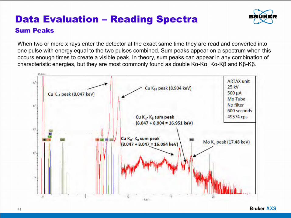
Data Evaluation – Reading Spectra Rayleigh (Elastic) Scattering

,QFLGHQW�UDGLDWLRQ�IURP�WKH�WXEH�WKDW�UHDFKHV�WKH�VDPSOH�LV�HLWKHU�DEVRUEHG�LQ�WKH�SKRWRHOHFWULF�HIIHFW�RU�UHIOHFWHG�DQG�VFDWWHUHG��:KHQ�DQ�[�UD\�UHIOHFWV�RII�WKH�DWRPV�RI�WKH�VDPSOH�ZLWKRXW�ORVLQJ�DQ\�HQHUJ\�LW�LV�FDOOHG�5D\OHLJK��RU�HODVWLF��VFDWWHULQJ��7KH�HQHUJ\�RI�WKH�RXWERXQG�[�UD\�ZLOO�EH�HTXDO�WR�WKH�HQHUJ\�RI�WKH�LQERXQG�[�UD\��WKXV�EHLQJ�GHWHFWHG�DV�D�VRXUFH�SHDN�ZLWK�WKH�HQHUJ\�RI�WKH�LQERXQG�[�UD\��7KH�5D\OHLJK�VFDWWHU�SHDNV�YLVLEOH�FRUUHVSRQG�ZLWK�WKH�FKDUDFWHULVWLF�HQHUJLHV�RI�WKH�[�UD\�WXEH�WDUJHW�HOHPHQW���

38�

Data Evaluation – Reading Spectra Compton (Inelastic) Scattering

,QFLGHQW�UDGLDWLRQ�ZLWK�VXIILFLHQW�HQHUJ\�WR�LRQL]H�DQ�LQQHU�VKHOO�HOHFWURQ�LQ�DQ�DWRP�GRHV�QRW�DOZD\V�FDXVH�IOXRUHVFHQFH��EXW�LQVWHDG�FDXVHV�DQ�H[FLWDWLRQ�ZLWKRXW�ORVLQJ�DOO�RI�LWV�HQHUJ\��,Q�WKHVH�LQWHUDFWLRQV��FDOOHG�&RPSWRQ�VFDWWHULQJ��D�[�UD\�VWULNHV�DQ�DWRP�DQG�ORVHV�HQHUJ\��FDXVLQJ�WKH�H[FLWHPHQW�RI�DQ�LQQHU�VKHOO�HOHFWURQ��%HFDXVH�QR�YDFDQF\�LV�FUHDWHG�LQ�WKH�DWRP��QR�FKDUDFWHULVWLF�HQHUJ\�LV�UHOHDVHG��KRZHYHU��WKH�[�UD\�ZLOO�ORVH�HQHUJ\�DQG�EH�VFDWWHUHG�LQ�DOO�GLUHFWLRQV��&RPSWRQ�VFDWWHU�[�UD\V�DSSHDU�DV�D�EURDG�SHDN�GHILQHG�E\�WKH�DQJOH�EHWZHHQ�WKH�LQFLGHQW�EHDP�DQG�WKH�GHWHFWRU�IRU�WKH�WDUJHW�FKDUDFWHULVWLF�[�UD\�ORZHU�LQ�HQHUJ\�WKDQ�5D\OHLJK�VFDWWHU�SHDNV�EHFDXVH�WKH\�RQO\�ORVH�D�VPDOO�DPRXQW�RI�HQHUJ\�LQ�WKH�H[FLWDWLRQ�RI�DQ�HOHFWURQ��7KH\�DUH�JHQHUDOO\�EURDG�GXH�WR�WKH�DUHD�RI�WKH�GHWHFWRU�DQG�WKH�DUHD�RI�WKH�H[FLWLQJ�EHDP��

39�

Data Evaluation – Reading Spectra Peak Overlaps

=Q�.Į�SHDNV��������SDUWLDOO\�RYHUODS�ZLWK�WKH�&X�.ȕ�SHDN��������WR�IRUP�D�µVKRXOGHU¶�RQ�WKH�&X�SHDN�LQVWHDG�RI�WZR�VHSDUDWH�SHDNV��

40�

Data Evaluation – Reading Spectra Peak Overlaps

0Q.E�SHDN�RYHUODSV�ZLWK�)H.D�SHDN��REVFXULQJ�0Q.E�SHDN�

41�

Data Evaluation – Reading Spectra Sum Peaks

:KHQ�WZR�RU�PRUH�[�UD\V�HQWHU�WKH�GHWHFWRU�DW�WKH�H[DFW�VDPH�WLPH�WKH\�DUH�UHDG�DQG�FRQYHUWHG�LQWR�RQH�SXOVH�ZLWK�HQHUJ\�HTXDO�WR�WKH�WZR�SXOVHV�FRPELQHG��6XP�SHDNV�DSSHDU�RQ�D�VSHFWUXP�ZKHQ�WKLV�RFFXUV�HQRXJK�WLPHV�WR�FUHDWH�D�YLVLEOH�SHDN��,Q�WKHRU\��VXP�SHDNV�FDQ�DSSHDU�LQ�DQ\�FRPELQDWLRQ�RI�FKDUDFWHULVWLF�HQHUJLHV��EXW�WKH\�DUH�PRVW�FRPPRQO\�IRXQG�DV�GRXEOH�.Į�.Į��.Į�.ȕ�DQG�.ȕ�.ȕ��

42�

Data Evaluation – Reading Spectra Escape Peaks

:KLOH�PRVW�FKDUDFWHULVWLF�[�UD\V�HQWHULQJ�WKH�GHWHFWRU�DUH�FRQYHUWHG�LQWR�SXOVHV�ZKLFK�DUH�SURFHVVHG�E\�WKH�GLJLWDO�SXOVH�SURFHVVRU��DQ�LQFRPLQJ�[�UD\�FDQ�H[FLWH�DQG�FDXVH�IOXRUHVFHQFH�LQ�DQ�DWRP�LQ�WKH�GHWHFWRU��,I�WKH�[�UD\�HQWHULQJ�WKH�GHWHFWRU�KDV�DQ�HQHUJ\�JUHDWHU�WKDQ�WKH�DEVRUSWLRQ�HGJH�RI�DQ�HOHPHQW�LQ�WKH�GHWHFWRU��IRU�WKH�7UDFHU��6LOLFRQ���WKHQ�IOXRUHVFHQFH�LQ�WKH�GHWHFWRU�PD\�RFFXU��7KH�LQERXQG�[�UD\�ZLOO�ORVH�WKH�DPRXQW�RI�HQHUJ\�UHTXLUHG�WR�IOXRUHVFH�WKH�GHWHFWRU�DWRP��OHDYLQJ�WKH�[�UD\�ZLWK�DQ�HQHUJ\�(¶ (�LQERXQG�±�(�&KDUDFWHULVWLF�HQHUJ\�RI�GHWHFWRU��WKXV�FDXVLQJ�WKH�GHWHFWRU�WR�UHDG�WKH�[�UD\�DV�KDYLQJ�DQ�HQHUJ\�RI�(¶����(VFDSH�SHDNV�DUH�PXFK�OHVV�LQWHQVH�WKDQ�WKH�FKDUDFWHULVWLF�SHDNV�IURP�ZKLFK�WKH\�DUH�GHULYHG��6HYHUDO�HVFDSH�SHDNV�FDQ�RFFXU�LQ�RQH�VSHFWUXP��JLYHQ�WKDW�DOO�FKDUDFWHULVWLF�HQHUJLHV�DERYH�WKH�DEVRUSWLRQ�HGJH�RI�WKH�GHWHFWRU�DUH�FDSDEOH�RI�FDXVLQJ�IOXRUHVFHQFH��,Q�WKH�FDVH�RI�D�6L�EDVHG�GHWHFWRU��HVFDSH�SHDNV�ZLOO�DSSHDU�DSSUR[LPDWHO\������NH9�ORZHU�WKDQ�D�FKDUDFWHULVWLF�SHDN�EHFDXVH�VLOLFRQ�KDV�D�.Į�DEVRUSEWLRQ�HGJH���

43�

Data Evaluation – Reading Spectra Escape Peaks

44�

Data Evaluation – Reading Spectra Instrument Artifacts

$V�WKH�LQFLGHQW�UDGLDWLRQ�WUDYHOV�IURP�WKH�VRXUFH�WR�WKH�VDPSOH��LW�PD\�FDXVH�IOXRUHVFHQFH�LQ�PDWHULDOV�LQ�WKH�LQVWUXPHQW�ZKLFK�PD\�EH�GHWHFWHG�DQG�VKRZQ�RQ�WKH�VSHFWUXP��7KH�WDUJHW�HOHPHQW�PD\�EH�GHWHFWHG��DV�ZHOO�DV�LURQ��]LQF��FRSSHU��DQG�QLFNHO�LQ�WKH�WXEH��FROOLPDWRUV��OHQV��HWF������;�UD\�WXEH�WDUJHW�.�DQG�/�OLQHV��H�J��5K�����6WDLQOHVV�6WHHO�'HWHFWRU�&DQ�/LQHV��H�J��)H��&R��1L��RQO\�DSSHDU�ZKHQ�WHVWLQJ�ORZ�=�HOHPHQWV�����:LQGRZ�OLQHV��H�J��&D�����&ROOLPDWRU�DQG�LQVWUXPHQW�VWUXFWXUH��H�J��3G�����,I�XVLQJ�D�WKLQ�ILOP�VDPSOH��HOHPHQWV�LQ�VXUIDFH�EHORZ�WKH�VDPSOH� %\�DGGLQJ�D�ILOWHU�LQ�EHWZHHQ�WKH�WXEH�DQG�WKH�VDPSOH��PXFK�RI�WKLV�XQZDQWHG�UDGLDWLRQ�FDQ�EH�UHPRYHG�IURP�WKH�VSHFWUXP� �

GEOCHEMICAL AND CHEMOSTRATIGRAPHIC APPLICATIONS OF XRF ANALYSIS

HARRY ROWE BUREAU OF ECONOMIC GEOLOGY

Geochemical�Model�for�Sample�Mineralogy

Si

SiO2 Quartz

Al

KAl2(SiO3AlO10)(OH)2 Illite

Fe FeS2Pyrite

Carbonates: siderite, ankerite, dolomite

CaSO4-2(H2O)Gypsum

Mg, MnCa CaCO3

Calcite

Ti AlWAYS detrital, regardless of originPhosphates: apatite, francolite, vivianite

%Ca

400 10 20 30

Depth(ft)

7100

7120

7140

7160

7180

7200

7220

%Ca

400 10 20 30

Depth(ft)

7100

7120

7140

7160

7180

7200

7220

%Al

0 2 4 6 8

%Ca

0 10 20 30 40

Depth(ft)

7100

7120

7140

7160

7180

7200

7220

Si/Al

0 5 10 15 20

%Al

0 2 4 6 8

Barnett�Shale,�SE�Wise�Co.,�TX

%Ca

0 10 20 30 40

Depth(ft)

7100

7120

7140

7160

7180

7200

7220

Si/Al

0 5 10 15 20

%Al

0 2 4 6 8

%Ca

0 10 20 30 40

Depth(ft)

7100

7120

7140

7160

7180

7200

7220

Si/Al

0 5 10 15 20

%Al

0 2 4 6 8

%Ca

0 10 20 30 40

Depth(ft)

7100

7120

7140

7160

7180

7200

7220

Si/Al

0 5 10 15 20

%Al

0 2 4 6 8

U. Barnett

L. SiliceousBarnett

L. ArgillaceousBarnett

Forestburg LSstrongcyclicity

� View�these�different�lithologies as�falling�somewhere�along�a�“clayͲcarbonate�continuum”……� And,�just�as�lithology/facies may�reflect�petrophysicalcharacteristics,�so�shall�the�“chemofacies”…which�may�be�a�more�quantitative�way�of�making�the�linkage�between�facies and�petrophysics….it�is�certainly�faster.� At�the�very�least,�chemostratigraphy brings�more�evidence�for/against�ideas�developed�through�faciesidentification/analysis.�

How�can�we�think�about�these�records?

Let’s�ThinkDeeper

� Problem�#1:�In�black�(or�any�color)�shales,�we�can’t�visually see�much�of�anything....� Problem�#2:�In�carbonates,�we�can’t�see�the�small�stuff�(diluted�by�fossils,�diluted�

by�overabundance�of�Ca)

� Best�thing�might�be�to�have�mineralogy�(XRD)—only�if�there�are�different�minerals.� Problem#3:�a)�Takes�too�long;�b) Everybody�does�it�slightly�differently,�leading�to�

variable�results;�c)�Biggest�problem�is�quantifying�clay�content�and�type.� Problem�#4:�While�shales/mudrocks have�diverse�mineralogies,�the�mineralogy�is�

overwhelmingly�calcite/dolomite�in�carbonates...that’s�why�they’re�called�carbonates.

� Solution:�Elemental�geochemistryͲͲspecifically,�a�geochemical�model�that�can�infer�and�be�checked with�mineralogy�(XRD).

� Bonus:�Some�elements�can�provide�additional�informationͲͲͲwhich�might�even�be�useful!�Example:�redoxͲsensitive�trace�elements�(RSTEs).

� Icing�on�the�cake:�Not�only�can�the�model�be�checked with�XRD,�but�elemental�geochemistry�can�tell�us�where�to�take�the�limited�XRD�samples.

Chemostratigraphy: Carthage Core, Panola Co., TX

Chemostratigraphy: Carthage Core, Panola Co., TX

Elemental BiPlots:Carthage Core, Panola Co., TX

� Ferroan and manganoan dolomite/ankerite

� Mild manganoan calcite� Most Fe is in clays

Elemental BiPlots:Carthage Core, Panola Co., TX

� Si-Al line demonstrates clay with quartz

� K and Ti can be used as detrital (clay) proxies

� V—mostly of detrital origin!!

� Zr and Al are not strongly linked, suggesting difference in transport or origin (grain size)

Chemostratigraphic Correlation: %Ca

�%Ca is high and upwardly descending in the Lower Haynesville chemofacies.

�%Ca is low and largely invariant in Middle Haynesville chemofacies.

�%Ca has an expanded range and is “jumpy” in the Upper Haynesville chemofacies.

Haynesville�Closer�Look(Huffman�Core,�Panola,�Co.,�TX)

%Ca

0 10 20 30 40

Dep

th(ft

)

10950

11000

11050

11100

11150

11200

Si/Al

0 1 2 3 4 5

Ti/Al

0.0 0.1 0.2

Ca/Al

0 10 20 30

%Ca

0 5 10 15 20 25 30

Dep

th(ft

)

10960

10980

11000

11020

11040

� Cause�of�cyclicity(cyclicities!)?

� Significance�for�depositional�environment�interpretations?

� Significance�for�understanding�highly�oscillatory�interͲbed�competency�and�building�the�petrophysical model.

TOC (%)0 1 2 3 4 5 6 7

Mo

(ppm

)

0

10

20

30

40

50

60

70

UppermostSample

LowermostSample

MoͲTOC�Relationship�in�the�Hay�Core

Integration�of�Logs�and�Chemostratigraphy

Integration�of�Logs�and�Chemostratigraphy


Recommended